Exploring Higher-Dimensional Black Holes in Numerical ...masaru.shibata/PTPS190.282.pdf ·...

282 Progress of Theoretical Physics Supplement No. 190, 2011

Exploring Higher-Dimensional Black Holes in Numerical Relativity

Hirotaka Yoshino1 and Masaru Shibata2

1Cosmophysics Group, Institute of Particles and Nuclear Studies, KEK,Tsukuba 305-0801, Japan

2Yukawa Institute for Theoretical Physics, Kyoto University,Kyoto 606-8502, Japan

We review the current status of our activity in higher-dimensional numerical relativ-ity. We describe a Baumgarte-Shapiro-Shibata-Nakamura formulation in higher dimensionstogether with cartoon methods which we employ. We also review numerical results whichwe derive for two subjects in higher-dimensional numerical relativity: dynamical instabil-ity of rapidly rotating Myers-Perry (MP) black holes with one rotational parameter andhigh-velocity black hole collisions and scatterings. The perspective for the future is brieflydescribed.

§1. Introduction

Numerical relativity is probably the unique approach for exploring dynamicalproblems in general relativity. In numerical relativity, Einstein’s equation,

Gab = 8πGTab, (1.1)

is numerically solved in the framework of an initial-value formulation of general rela-tivity. In the past decade, the community of numerical relativity achieved significantprogress, and now, it is feasible to perform a longterm and accurate simulation forthe merger of binary composed of black holes and neutron stars (e.g., Refs. 1)–6) forbinary black holes and Ref. 7), 8) for others) and for high-velocity collision of twoblack holes, that are among the strongest gravitational phenomena in nature.

Higher-dimensional numerical relativity is also being an important issue sincethe TeV gravity scenarios9)–12) and the AdS/CFT correspondence13) were proposed.To clarify the nonlinear dynamics in higher-dimensional general relativity, a newimplementation in numerical relativity is necessary. Higher-dimensional numericalrelativity began in 2003 by a pioneering simulation for a 5-dimensional (5D) blackstring that is unstable against the Gregory-Laflamme instability.14),15) Then, severalnew formulations have been developed and several simulations have been performedin particular in the last three years.

There are three primary motivations for performing higher-dimensional numer-ical relativity. The first one is stimulated by the fact that mini black holes maybe produced in large accelerators such as Large Hadron Collider (LHC) if the TeVgravity hypotheses are correct. If our 3-dimensional (3D) space is a D3-brane inlarge9),10) or warped11) extra dimensions, the Planck energy could be of O(TeV) andquantum gravity phenomena may emerge in high-energy particle colliders. If theparticle energy is larger than the Planck energy in this scenario, mini black holescould be produced16)–18) (see also Ref. 19) for a recent review). If a black hole with

Higher-Dimensional Numerical Relativity 283

mass energy slightly larger than the Planck energy is formed in the LHC, it will sub-sequently emit the Hawking radiation that may be detected. To accurately predictthe rate of the mini black-hole production and its detectability, it is necessary toknow the cross section for the black-hole production σBH, and the resulting massand angular momentum of the formed black hole. A lower bound of σBH for theblack-hole production was given in Refs. 20) and 21) by numerically solving the ap-parent horizon at an instance of the collision of Aichelburg-Sexl particles22) in higherdimensions (see also Ref. 23)). However, the precise value of σBH and the black-holeproduction rate are necessary for precisely predicting the event rate in the particlecollider.

The second motivation is to clarify the fundamental properties of black objectsin higher dimensions. 4-dimensional (4D) black holes (Kerr black holes) have beenshown to be stable in vacuum irrespective of its mass and spin. By contrast, higher-dimensional black objects are not always stable. For example, the Gregory-Laflammeinstability24) is known for a black string. Also, higher-dimensional rapidly rotatingblack holes (i.e., the Myers-Perry (MP) black holes25)) are unstable,26)–29) and ablack hole on a Randall-Sundrum (RS) brane is also conjectured to be unstable.30)

The condition for the onset of the instabilities and the final fate after their onset areclarified only in numerical relativity (see §3).

The third motivation comes from the hypothesis of the AdS/CFT correspon-dence, which conjectures that the classical gravity of anti-de Sitter (AdS) spacetimeis dual to the conformal field theory (CFT) on the boundary of the AdS spacetime.If this hypothesis holds, we may be able to obtain an idea for phenomena in CFT, forwhich explicit calculations are difficult due to the strong coupling effect, by studyingthe dual gravitational system. To calculate time-dependent phenomena in the grav-ity side which is expected to be dual to the CFT phenomena of interest, numericalrelativity will play an important role.

The purpose of this article is to review our activity in higher-dimensional numer-ical relativity. In §2, we review the Baumgarte-Shapiro-Shibata-Nakamura (BSSN)formulation for higher-dimensional numerical relativity together with the “cartoonmethods” for implementing spacetime symmetries, that are employed in our numeri-cal code. In §3, we summarize several test simulations which are useful for validatingnumerical codes, illustrating that our codes are validated by these test simulations.In §4, we review the simulation results obtained by our group, focusing in particu-lar on the numerical results for rapidly rotating Myers-Perry (MP) black holes thatmay be dynamically unstable against nonaxisymmetric deformation (§4.1) and high-velocity two-black-hole collisions in a 5D spacetime (§4.2). Section 5 is devoted to asummary and a brief discussion of the issues for the future. Throughout this arti-cle, the unit c = 1 is used, while the higher-dimensional gravitational constant G isexplicitly shown.

§2. Formulation

There are many ingredients necessary for a successful simulation of vacuumspacetimes in numerical relativity: formulations including methods for implementing

284 H. Yoshino and M. Shibata

spacetime symmetries for a special class of spacetime; appropriate gauge conditions;methods for extracting gravitational waves; techniques for handling black holes; ap-parent horizon (AH) finder; adaptive mesh refinement (AMR). These ingredientswere already developed in 4D numerical relativity. Most of them can be extendedfor higher-dimensional numerical relativity in a straightforward manner. In this sec-tion, we describe the methods of the extension of the BSSN formulation togetherwith the cartoon methods. For a summary of other formulations, we recommend thereader to refer to Ref. 31).

2.1. BSSN formulation

In 4D numerical relativity, the BSSN formulation32),33) is most popular for alongterm and stable simulation, and its extension for higher-dimensional numericalrelativity is straightforward.34) The BSSN formulation is in a sense a modifiedversion of the ADM formulation;35) the numerical stability is realized by a suitablemodification of the ADM formulation. In the following, we briefly review the ADMand the BSSN formulations for D-dimensional spacetimes.

Suppose M be a D-dimensional spacetime with a metric gab. Consider a se-quence of N -dimensional spacelike hypersurfaces Σt(hab,Kab) foliated by a time co-ordinate t in M.∗) Here, hab is the induced metric hab := gab + nanb of Σt, wherena is the future-directed unit normal Σt, and Kab is the extrinsic curvature definedby Kab := −(1/2)£nhab, where £n is the Lie derivative with respect to na. Thecoordinate basis ta of the time coordinate t is decomposed as ta = αna + βa, whereα and βa are the lapse function and the shift vector, respectively. In terms of thesevariables, the metric is written in the form

ds2 = −α2dt2 + hij(dxi + βidt)(dxj + βjdt), (2.1)

and Einstein’s equation in the coordinate basis is rewritten as

R+K2 −KabKab = 16πGρ, (2.2)

DbKba −DaK = 8πGja, (2.3)

£thab = −2αKab +Daβb +Dbβa, (2.4)

£tKab = −DaDbα+ α(R

(Σ)ab − 2KacK

cb +KabK

)+ βcDcKab +KbcDaβ

c +KacDbβc − 8πGα

[Sab +

ρ− S

D − 2hab

], (2.5)

where Eq. (2.4) is equivalent to the definition of Kab, and Eqs. (2.2), (2.3), and (2.5)are derived from Gabn

anb = 8πGρ, Gbcnbhc

a = −8πGja, and Gcdhcah

db = 8πSab

using Gauss, Codazzi, and Ricci equations, respectively. Here, we defined

ρ := Tabnanb; ja := −Tbcn

bhca; Sab := Tcdh

cah

db, (2.6)

∗) Latin indices a, b, c, · · · are the abstract indices, while i, j, k, · · · denote the components in

the coordinate basis.


and S := Scc. R

(Σ)ab denotes the Ricci tensor with respect to hab.

Equations (2.2) and (2.3) are Hamiltonian and momentum constraint equations:On the initial spacelike hypersurface (i.e., initial data), these two constraints have tobe satisfied. Then, the time evolution of (hij ,Kij) is determined by Eqs. (2.4) and(2.5). The constraint equations are automatically satisfied after the time evolutionas long as the evolution equations are solved exactly. However, these constraints arealways violated slightly in actual simulations. The violation does not grow with timeonly in an appropriate formulation, which is necessary in numerical relativity. TheBSSN formulation is one of the most popular formulations with which the constraintviolation is well controlled.

The basic idea of the BSSN formulation is to increase the number of variables aswell as that of constraints to suppress the growth of unphysical modes. Specifically,new variables, χ, hij , Aij , and Γ i, are defined from

hij = χhij , Kij =1χ

(Aij +

K

Nhij

), Γ i := hjkΓ i

jk = −hik,k. (2.7)

Here, the conformal factor χ is chosen so that the determinant h of hij satisfies thecondition in the Cartesian coordinates

h = 1, (2.8)

which is equivalent to setting χ = h−1/N , and Γ ijk denotes the Christoffel symbol

with respect to hij . The evolution equations are derived as

(∂t − βi∂i)χ =2Nχ(αK − ∂iβ

i), (2.9)

(∂t − βi∂i)K = −DiDiα+ α

(AijAij +

K2

N

)+

8παD − 2

[(D − 3)ρ+ S] , (2.10)

(∂t − βj∂j)Γ i = −2Aij∂jα+ 2α[Γ i

jkAjk − D − 2

NhijK,j − 8πhijjj − Nχ,j

2χAij

]

− Γ j∂jβi +

2NΓ i∂jβ

j +D − 3N

hikβj,jk + hjkβi

,jk. (2.11)

(∂t − βk∂k)hij = −2αAij + hik∂jβk + hjk∂iβ

k − 2N∂kβ

khij , (2.12)

(∂t − βk∂k)Aij = χ[−(DiDjα)TF + α

(R

(Σ)TFij − 8πSTF

ij

)]+ α

(KAij − 2AikA

kj

)+ Aik∂jβ

k + Akj∂iβk − 2

N∂kβ

kAij , (2.13)

where the indices of Aij are raised and lowered by hij , and TF denotes the trace-freepart, e.g., R(Σ)TF

ij = R(Σ)ij − R(Σ)hij/N . The Ricci tensor is decomposed into two

parts asR

(Σ)ij = Rij +R

(χ)ij , (2.14)


where Rij is the Ricci tensor with respect to hij and R(χ)ij is the remaining part

composed of the conformal factor, written in the form

Rij = −12hklhij,kl +

12

(hki∂jΓ

k + hkj∂iΓk)

−12

(hil,kh

kl,j + hjl,kh

kl,i − Γ lhij,l

)− Γ l

ikΓkjl, (2.15)

R(χ)ij =

(D − 3)2χ

(χ,ij − Γ k

ijχ,k

)− (D − 3)

4χ,iχ,j

χ2

+hij hkl

[χ,kl

2χ− Nχ,kχ,l

4χ2

]− 1

2hij

χ,m

χΓm. (2.16)

The second derivatives of hij appear only in the first term of Eq. (2.16) (i.e., eachcomponent of hij appears to obey a simple wave equation) and this is the key pointfor the numerical stability.

In summary, the variables to be evolved are χ, K, hij , Aij , and Γ i, and theyfollow Eqs. (2.9), (2.10), (2.12), (2.13), and (2.11), respectively. The conditionsAi

i = 0, third equation of Eq. (2.7), and Eq. (2.8) are regarded as the new constraintswhich arise because the number of the dynamical variables are increased. As shownabove, the BSSN formulation for higher dimensions has essentially the same form asthat for the 4D case, except that some coefficients are changed.

2.2. Cartoon method

In the presence of spatial symmetries, it is better to impose such symmetries innumerical simulation to reduce computational costs. In the previous subsection, theBSSN formulation was described assuming that the Cartesian coordinates are usedand without assuming the presence of any symmetries a priori. In this subsection, wedescribe the so-called cartoon method for imposing symmetries in such a formulation.

2.2.1. Cartoon methodThe cartoon method was originally proposed by Alcubierre et al.36) as a pre-

scription for an efficient numerical simulation of axisymmetric 4D spacetimes. Theessence in this method is to employ not curvilinear coordinates that possess coordi-nate singularities, but the Cartesian coordinates. First of all, we briefly review theoriginal idea of the cartoon method.

In an axisymmetric 3D space, the Cartesian coordinates (x, y, z) are introducedso that the z-axis becomes the symmetry axis of axisymmetry (U(1) symmetry) (werefer to this case as “x = y, z” which indicates that the spatial structures in the xand y directions are equivalent). In the Cartesian coordinates, the U(1) symmetrydoes not explicitly appear in equations, and we cannot evolve the geometric variablesstraightforwardly only with the data on, e.g., the (x, z)-plane because y derivativesof them are needed. In the originally cartoon method, a few grid points in theneighborhood of the (x, z)-plane are prepared. Then, the data at a grid point (x, y �=0, z) is generated using the data at a point (ρ, 0, z) (i.e., on the (x, z)-plane) whereρ =

√x2 + y2, using the U(1) symmetry. Here, an appropriate interpolation has

to be done because the point (ρ, 0, z) is not located on a grid in general. Once the


data at the grid points y �= 0 are known, y derivatives at y = 0 are calculated andthe data on the (x, z)-plane is evolved toward the next time step. The symmetricrelation is α(x, y, z) = α(ρ, 0, z) for a scalar function, and those for vector and tensorfunctions are also derived by the relations that the Lie derivative of functions withrespect to the Killing vector becomes zero.

We described the method for extensions of the cartoon method to 5D space-times (4D spaces) in the cases of three types of symmetries, i.e., the U(1) symmetry(“x, y, z = w”), the U(1)×U(1) symmetry (“x = y, z = w”), and the O(3) symme-try (“x = y = z, w”) denoting the Cartesian coordinates by (x, y, z, w).34) For theU(1) symmetry, the extension is straightforwardly done. The cartoon method forthe U(1)×U(1) symmetry is similar to that for the U(1) symmetric case except thattwo cartoon operations are required in this case. In the case of the SO(3) symmetry,the symmetric relations are different from that for the U(1) symmetric case, butthey can be derived in a similar manner (see Ref. 34) for details).

2.2.2. Modified cartoon methodIn the original cartoon method, we have to prepare the extra grids in all the

symmetric directions. For this reason, as the dimensionality D is increased by 1, therequired grid number always increases by a factor of 5 (if we use the 4th-order finitedifferencing), and thus, a lot of memories are still required for a large value of D.However, this can be avoided by a prescription shown below.29)

As an example, we here consider an N -dimensional space with the coordinates(x, y, z, w1, ..., wn) where n = D − 4, and suppose that this space has the O(D −3) symmetry with respect to (z, w1, ..., wn) (i.e., “z = w1 = · · · = wn”). Thesimulation is supposed to be performed on the (x, y, z)-plane. Here, we introduce

ρ =√z2 +

∑ni=1w

2i , and in the following, indices a and b denote x or y. The

symmetric relation of a scalar function is

α(x, y, z, wi) = α(x, y, ρ, 0), (2.17)

and from this relation, the derivatives are evaluated as

α,wi = α,awi = α,zwi = 0, α,wiwj = (α,z/z)δij. (2.18)

The derivatives of vector and tensor functions with respect to wi can be derived ina similar way using the symmetric relations. Then, all the derivatives necessary forsolving the evolution equations can be evaluated without preparing the extra grids.The derivatives with respect to wi are replaced with those to z or a simple algebraicrelation. This implies that additional finite differencing operation is absent. Due tothis fact, the computational costs do not increase significantly with this prescription,and the simulation is effectively performed in the 3 + 1 manner, as in the case thatwe employ curvilinear coordinates.

§3. Method for code validation

To confirm the reliability of a code newly developed, benchmark tests are nec-essary. One of the standard tests is to check the convergence of numerical results


with varying grid resolutions: The numerical solution has to show a convergenceproperty that is expected in the employed scheme. Another method is to simulate aspacetime for which an analytic (or semi-analytic) solution is known and to confirmthat the numerical results agree with the analytic solution. Here, we summarizethe 5D spherically symmetric black hole spacetime in the Gaussian normal coordi-nates which is useful for the benchmark tests, and show that our code accuratelyreproduces the solution.

3.1. Geodesic slice of Schwarzschild-Tangherlini spacetime

First, we show an analytic solution of the 5D spherical black hole in the geodesicslicing. The well-known metric form of this black hole (the so-called Schwarzschild-Tangherlini metric) is

ds2 = −f(r)dt2 +dr2

f(r)+ r2dΩ2

3 , f(r) = 1 − r2Sr2, (3.1)

where dΩ23 is the line element of a 3D unit sphere and rS is the Schwarzschild-

Tangherlini radius rS =√

8GM/3π. Because the coordinates in this metric are notwell-behaved inside the event horizon, we rewrite the metric of this spacetime interms of the Gaussian normal coordinates starting from the t = 0 hypersurface as

ds2 = −dτ2 +

[r20 + (rS/r0)2τ2

]2[r20 − (rS/r0)2τ2

] dR2

R2+[r20 − (rS/r0)

2 τ2]dΩ2

3 , (3.2)

where r0 is defined by

r0 = R

(1 +

r2S4R2

). (3.3)

The spacetime domain which these coordinates cover is explained as follows. Con-sider a geodesic congruence of test particles that are initially at rest. Then, eachgeodesic labels the radial coordinate and its proper time is equal to the time coordi-nate. At τ = 0, the spatial slice agrees with the Einstein-Rosen bridge written withthe isotropic radial coordinate R. This is analogous to the Novikov coordinates inthe 4D Schwarzschild spacetime.37),38) This line element shows that the RR com-ponent of the metric grows and diverges at τ = r20/rS , at which the slice hits thesingularity.

In the line element (3.2), τ and R are always time and radial coordinate, andthus, this coordinate system can be employed in numerical relativity. In this test, asimulation is done with the gauge conditions α = 1 and βi = 0, until the computationcrashes approximately at the crash time τcrash = rS . Figure 1 shows a comparisonbetween the analytic solution (solid curves) and the data34) with grid size Δx/rS =0.1 (crosses, ×) and 0.05 (circles, �). Here, the snapshots of xx component of theconformal 4D metric hxx along the x-axis are drawn for τ/rS = 0.5, 0.6, 0.7, 0.8, and0.9. This shows that the numerical solutions agree approximately with the analyticsolutions (3.2) (solid curves): The values of hxx rapidly increase and blow up aroundx = 1. It is also checked that the deviation of the numerical solutions from theanalytic one shows the 4th-order convergence in a code implementing a 4th-orderfinite differencing.34)


Fig. 1. Snapshots of hxx along the x-axis for τ/rS = 0.5, 0.6, 0.7, 0.8, and 0.9. The unit of x is

rS/2. The grid resolutions are Δx = 0.1 (×) and 0.05 (�). The solid curves denote the analytic

solutions. The figure is taken from Ref. 34).

Fig. 2. The sequence of maximal slicing surfaces in the Kruskal diagram of the Schwarzschild-

Tangherlini spacetime for D = 5. The dotted curves show the r = const. The limit surface is

given by r =p

2/3rS . The figure is taken from Ref. 41).

3.2. Limit surface of Schwarzschild-Tangherlini spacetime

As the second analytic solution, we refer to the limit surface of the maximallysliced evolution (i.e. evolution keeping K = 0) of a Schwarzschild-Tangherlini space-time. In the 4D Schwarzschild black hole, it was shown that the sequence of themaximal slices never hits the curvature singularity but asymptotes to the so-calledlimit surface,39) for which an analytical expression of the limit surface, suitable innumerical relativity, was given, e.g., in Ref. 40). The limit surface provides a usefultest-bed for calibrating numerical-relativity codes because it is a stationary solutionfor the black hole. Namely, if we adopt the limit surface as the initial data, thespacelike hypersurface has to be unchanged during the time evolution under certaingauge conditions.

The limit surface for the higher-dimensional black hole is derived by Nakao etal.41) Figure 2 displays the Kruskal diagram of the 5D Schwarzschild-Tangherlinispacetime. The sequence of maximal-sliced hypersurfaces (starting from the time-symmetric slice) is shown by the solid curves. The sequence asymptotes to r =


Fig. 3. The analytic solutions of α, βx, Ayy, and χ along the x-axis for the limit surface of the 5D

spherical black hole (solid curves), and the numerical data after the time evolution at t = 50rS

(�). Here, the unit of the length is rS/2. The data remains approximately stationary in the

time evolution. The figure is taken from Ref. 34).

√2/3rS , which is the limit surface, and the formula for the limit surface can be

given analytically also in the 5D case. The limit surface turns out to be conformallyflat, and thus, we can introduce the spherical-polar coordinates (R, φi) in the flatspace. The relation between R and the Schwarzschild radial coordinate r is

R =r

6

(3 +

√3 [(rS/r)2 + 3]

)( (5 + 2√

6)[3 − 2(rS/r)2

]2(rS/r)2 + 15 + 6

√2 [(rS/r)2 + 3]

)1/√

6

. (3.4)

In terms of the BSSN variables,

χ =(R

r

)2

, α =

√1 −

(rSR

)2χ+

427

(rSR

)6χ3, (3.5)

βR =2

3√

3χ2(rSR

)3, AR

R = −3Aφi

φi= − 2√

3χ2 r

3S

R4. (3.6)

Here, r has to be written as a function of R numerically, and then, the nontrivialcomponents can be calculated.

Figure 3 plots the values of α, βx, Ayy, and χ along the x-axis at a selected timeslice. Adopting the data shown by the solid curves as the initial condition, we evolvedthis spacetime using the dynamical gauge condition together with Γ -driver.34) Thedata at t = 50rS (after the time evolution) are plotted by the circles. It is confirmedthat all the BSSN variables are approximately unchanged in time. In this manner,we can check the reliability of the code using the limit surface solution.


§4. Simulations

In this section, we review our numerical results for two subjects in higher-dimensional numerical relativity: One is on the bar-mode instability of rapidly ro-tating Myers-Perry (MP) black holes with one rotational parameter28),29) and theother is on high-velocity black-hole collisions.42)

4.1. Bar-mode instability of Myers-Perry black holes

The MP black holes have been inferred to be unstable against certain perturba-tions.26),27) The dynamical instability of rapidly rotating Myers-Perry (MP) blackholes with one spin parameter25) was explored in Refs. 28), 29) by fully nonlinearsimulations, and it was shown that the MP black holes are indeed dynamically un-stable if they are rotating sufficiently rapidly, and that the most unstable mode isthe bar-mode.28),29) In this subsection, we review this study.

4.1.1. The Myers-Perry black holesIn D-dimensional spacetimes, the spacetime can have �(D − 1)/2� independent

rotational parameters (i.e., the independent components of angular momentum ten-sor) where �x� indicates the largest integer not greater than x. The black holesolutions of spherical horizon topology with arbitrary number of rotational parame-ters in higher-dimensions were found by Myers and Perry.25) Hereafter, we consideronly MP black holes with one spin parameter for which the metric is given by∗)

ds2 = −dt2+ μ

Σ(dt−a sin2 θdϕ)2+

Σ

Δdr2+Σdθ2+(r2+a2) sin2 θdϕ2+r2 cos2 θdΩ2

D−4,

(4.1)where

Σ = r2 + a2 cos2 θ, Δ = r2 + a2 − μ/rD−5. (4.2)

In this case, the spacetime has a U(1) symmetry with respect to the rotational planeand an O(D−4) symmetry with respect to the directions orthogonal to the rotationalplane. μ and a are related to the mass M and angular momentum J by

M =(D − 2)ΩD−2μ

16πG, J =

2(D − 2)

Ma. (4.3)

The location r = rK(M,J) of the event horizon is given by the equation Δ(rK) = 0.For D = 5, the event horizon exists only for a < μ1/2, whereas it exists for any valueof a for D ≥ 6.

4.1.2. Previous studiesFirst, we summarize the history for the stability analysis of the MP black hole. A

standard method for this is a linear perturbation study. If the variables of the linearperturbation equations are separable, the resulting equation reduces to an ordinarydifferential equation and its analysis may be done analytically or semi-analytically.Although linear perturbation equations in the MP spacetime have been extensivelystudied for a metric perturbation, the separation of the variables was succeeded only

∗) In this section, we use the units of G = 1 = c.


for a tensor-mode perturbation.49),50) For other modes, the stability has not beenfound yet by this analysis.

The next best method may be to numerically solve partial differential equationsfor linear perturbation equations without carrying out the separation of the variables.The first numerical analysis was done by Dias et al.27) In this study, an axisymmetricperturbation (i.e., the perturbation that keeps the U(1) × O(D − 4) symmetry)was studied and 2D simultaneous partial differential equations were solved. Theydiscovered that MP black holes with the ultra high spin (a� μ1/(D−3)) are unstableagainst axisymmetric deformation. However, no numerical study has been done fornonaxisymmetric perturbation that breaks the U(1) symmetry.

Alternatively, Emparan and Myers analyzed the stability of MP black holes usingtwo different analysis methods.26) In one analysis, they take the so-called blackmembrane limit of ultra spinning MP black holes. The ultra spinning MP blackholes for D ≥ 6 with a� μ1/(D−3) become extremely oblate. For such an extremelyoblate black object, instabilities analogous to the Gregory-Laflamme instability areexpected to set in. This discussion was applied to axisymmetric instabilities, andindeed, the numerical analysis of Dias et al. confirms this prediction.27)

The other analysis was based on black-hole thermodynamics: They comparedthe horizon area of a rotating MP black hole with that of two boosted Schwarzschild-Tangherlini black holes, which recede from each other, fixing the total gravitationalenergy and angular momentum. The horizon area of a MP black hole is

AMP = ΩD−2rD−2K

(r2K + a2

), (4.4)

whereas sum of the area of two boosted black holes is

2AS = 2ΩD−2rS(m)D−2, (4.5)

where rS(m) is the horizon radius of a Schwarzschild-Tangherlini black hole. Here,the ADM mass M and the mass m of each black hole are related as M = 2

√m2 + p2

where p is the magnitude of the momentum of each black hole. The angular mo-mentum of the system J is given by J = bp, where b is an “impact parameter”, i.e.,the distance between two black holes in the direction orthogonal to the momenta,chosen to be b ∼ rS(M) as a typical value. If AMP < 2AS , the configuration of twoboosted black holes may be preferred to the MP black hole thermodynamically. Ifthis is the case, it is expected that the MP black hole becomes unstable against non-axisymmetric perturbation, the horizon may pinch off, and the system may changeto a state of two boosted black holes. By this discussion, the MP black holes arepredicted to be unstable for

q := a/μ1/(D−3) � 0.85 (D = 5), 0.96 (D = 6), 0.99 (D = 7), 1.00 (D = 8).(4.6)

Here, we introduced a non-dimensional rotational parameter q which is used later.In contrast to the former discussion, this discussion can be applied to D = 5 as wellas D ≥ 6, and the predicted critical parameter for the onset of the instability is muchsmaller than that for the Gregory-Laflamme-like axisymmetric instability (i.e., theinstability can set in for a smaller black hole spin). Therefore, the nonaxisymmetricperturbation was predicted to be the primary instability.


4.1.3. Setup of the problemThe prediction by Emparan and Myers seems to be qualitatively correct. How-

ever, for strictly verifying that the instability sets in and for quantitatively clarifyingthe criterion for the onset of the instability, we have to solve Einstein’s equation,which can be done only by a numerical-relativity simulation. In the following, wereview our latest work.

The simulation was done in the following procedures. First, the MP black holewas written in the quasi-isotropic coordinates in which the radial coordinate is de-fined by

r = rh exp

[±∫ r

rK

dr′√r′2 + a2 − μ/r′(D−5)

]. (4.7)

This is analogous to the isotropic coordinates of the Schwarzschild-Tangherlini space-time (i.e., the radial coordinate for which the spatial part of the metric becomes con-formally flat), and the initial spacelike hypersurface possesses two asymptotically flatregions and one throat (i.e., the structure similar to the Einstein-Rosen bridge). Inthis quasi-isotropic coordinates, the horizon is located at r = rh. This spacelikehypersurface does not cross the physical curvature singularity of the MP spacetime.Then, the initial data is written in the (x, y, z, wi) coordinates

x = r cos θ cosφ, y = r cos θ sinφ,√z2 +

∑i

w2i = r sin θ, (4.8)

where the (x, y)-plane corresponds to the plane of the rotation.Next, a small nonaxisymmetric perturbation is added to the conformal factor of

the BSSN variables, χ, as

χ = χ0

[1 +Aμ−1(x2 − y2) exp(−r2/2r2K)

], (4.9)

where χ0 is the value of unperturbed initial data, and A is a small number 1.This perturbation breaks the U(1) symmetry with respect to (x, y)-plane and keepsthe O(D − 4) symmetry with respect to z and wi directions.

Adopting the initial data, we evolved the system by SACRA-ND code, which isa higher-dimensional version of SACRA code.51) This code employs the 4th-orderfinite differencing in space and the 4th-order Runge-Kutta method in time with anAMR algorithm. The modified version of the cartoon method explained in §2.2.2 isemployed to impose the O(D−4) symmetry. The so-called puncture gauge conditionwas adopted, and the parameters of the gauge conditions were carefully chosen forstable simulations (see Refs. 28), 29) for details).

4.1.4. Numerical resultsThe left panel of Fig. 4 shows gravitational waveforms of m = 2 mode extracted

in a local wave zone as a function of a retarded time for D = 5. For q � 0.85,the amplitude exponentially damps with t for t ≥ 8μ1/2. This shows that the blackhole is stable. By contrast, the amplitude for q � 0.87 remains approximatelyconstant, and that for q � 0.89 grows exponentially in time. This implies that


Fig. 4. Left panel: h+ and its absolute value as functions of retarded time for a/μ1/2 = 0.85, 0.87,

and 0.89 (dashed, long-dashed, and solid curves) for 5D MP black holes. Right panel: Evolution

of distortion parameter η of the apparent horizon for q = 0.80–0.89. The figures are taken from

Ref. 28).

Fig. 5. Left panel: Time evolution of a distortion parameter η for D = 6 and for the initial spin

qi = a/μ1/3 ≈ 1.039, 0.986, 0.933, 0.878, 0.821, 0.801, 0.781, 0.761, 0.750, 0.740, 0.718, and

0.674 (from the upper to lower curves) with A = 0.005. Right panel: The same as the left panel

but for D = 7 and for qi = a/μ1/4 = 0.960, 0.903, 0.844, 0.813, 0.783, 0.767, 0.751, 0.735, and

0.719 (from the upper to lower curves). The figures are taken from Ref. 29).

for q > 0.87 the black hole is unstable against nonaxisymmetric deformation. Theright panel of Fig. 4 shows the evolution of a distortion parameter η, defined byη := [(l0 − lπ/2)2 + (lπ/4 − l3π/4)2]1/2/l0 where lϕ denotes the proper circumferentiallength between θ = 0 and π/2 for a fixed value of ϕ evaluated on the apparenthorizon. This parameter indicates the degree of deviation from the axisymmetry,with η = 0 for an axisymmetric surface. As the figure shows, the value of η growsexponentially for q � 0.87, while η damps for q � 0.86. This also shows thatthe rapidly rotating black hole with q � 0.87 is unstable against nonaxisymmetricdeformation. The critical parameter for the onset of the instability is qcrit � 0.87.

Figure 5 shows the time evolution of the distortion parameter η for D = 6 (leftpanel) and D = 7 (right panel). Here, the definition of η is slightly modified asη := 2[(l0 − lπ/2)2 + (lπ/4 − l3π/4)2]1/2/(l0 + lπ/2). As in the 5D case, the value of η


Table I. The values of the critical rotational parameter qcrit for the onset of the bar-mode instability

for D = 5–8.

D 5 6 7 8

qcrit 0.87 0.74 0.73 0.77

Fig. 6. Left panel: + modes of gravitational waveform (solid curve) emitted from an unstable black

hole for D = 6 and for qi = 0.801 as a function of a retarded time defined by t − r where r is

the coordinate distance from the center. η/2 is also plotted as a function of t (dashed curve).

Right panel: The same as the left panel but for qi = 0.986. The figures are taken from Ref. 29).

exponentially damps in time if q is small, but it grows exponentially for q larger thana certain critical parameter qcrit. The value of qcrit is � 0.74 and 0.73 for D = 6 and7, respectively. The critical parameter qcrit for the onset of the instability is muchsmaller than that for the onset of the axisymmetric instability reported in Ref. 27)irrespective of dimensionality D. The results are summarized in Table I.

The solid curves of Fig. 6 plot gravitational waveforms in the longterm simula-tions where the initial value of q is qi = 0.801 (left panel) and 0.986 (right panel)for D = 6. The amplitude of gravitational waves grows in time in the early phaseand then saturates when the distortion parameter becomes of order 0.1 at t = tpeak.After the saturation, the amplitude exponentially damps. The reason is as follows.Associated with the growth of the nonaxisymmetric deformation, emissivity of grav-itational waves is enhanced, and energy and angular momentum are significantlyextracted from the black hole (although the area increases). As a result, the value ofthe non-dimensional spin parameter q decreases, and eventually, it becomes q � qcritwhen the growth of the amplitude saturates at t = tpeak. Gravitational waves con-tinue to extract energy and angular momentum even after the saturation and thefinal state is a stable state with the value of q = qf which is smaller than qcrit. Thetime, t = tpeak, for qi = 0.986 is smaller than that for qi = 0.801. This is because thegrowth rate of the instability for qi = 0.986 is larger than that for qi = 0.801, andtherefore, energy and angular momentum are extracted more efficiently. The dashedcurves of Fig. 6 plot half of the distortion parameter η of the apparent horizon. Itagrees approximately with the amplitude of gravitational waves, indicating that thedistortion of the apparent horizon is not due to a gauge mode and gravitationalwaves are generated by the distortion of the system.

Figure 7 shows the real part of the gravitational-wave frequency as a function


Fig. 7. Real part of gravitational-wave frequencies ω/m (where m = 2) for selected values of the

spin parameter for D = 5 – 7 (points) together with ΩH as a function of q = a/μ1/(D−3) for

D = 5 – 7 (from the upper to lower solid curves). The units of the vertical axis are μ−1/(D−3).

The values q = qcrit for the onset of the bar-mode instability are also shown for D = 5 – 7 (from

the right to left dotted lines). The figure is taken from Ref. 29) with modification.

Fig. 8. Left panel: The growth rate 1/τ of η in units of μ−1/(D−3) as a function of q (solid curve)

for D = 6. The dashed curve denotes ΩH/2π. Right panel: The same as the left panel but for

D = 7. The figures are taken from Ref. 29).

of q for D = 5, 6, and 7. The curve for the superradiance condition52) ω ≤ mΩH isalso shown for each value of D, where m = 2 and ΩH is the angular velocity of thehorizon. It is well known that the superradiance condition is the condition such thatwaves can extract energy and angular momentum from a black hole without violatingthe area theorem by Hawking. The superradiance condition is a necessary conditionfor subtracting energy from the black hole by waves. However, it is only a necessarycondition and not the sufficient condition for the onset of the dynamical instabilityfound in Refs. 28),29). In the superradiance often discussed, one considers to injectrather an artificial ingoing wave for which the frequency satisfies this condition.For such an artificial wave, the reflected waves are amplified. For the dynamicalinstability to occur, gravitational waves have to be spontaneously excited by unstable


Fig. 9. Left panel: Time evolution of Cp/Ce for D = 6 and for non-dimensional spin parameters

not much greater than qcrit, qi = a/μ1/3 = 0.821, 0.801, and 0.781. The corresponding initial

values of Cp/Ce are ≈ 0.587, 0.602, and 0.618, respectively. The results with A = 0.02 and 0.005

are plotted for qi = 0.801, and the results with A = 0.02 are plotted for qi = 0.821 and 0.781.

The solid and dashed curves denote the results for high and low resolution runs, respectively.

The thin dotted line denote Cp/Ce = 0.647 which is the value of Cp/Ce for q = qcrit. For

qi = 0.821, the simulation was stopped at t/μ1/3 ≈ 370 because the black hole reaches an

approximately stationary state. Right panel: The same as the left panel but for the large initial

spins qi = 0.878, 0.933, 0.986, and 1.039 with A = 0.005. Cp/Ce ≈ 0.542, 0.499, 0.460, and

0.422 at t = 0, respectively. The figures are taken from Ref. 29).

quasinormal modes. Namely, such a mode has to satisfy not only the superradiancecondition but also the condition that the imaginary part of the quasinormal mode isnegative. Figure 8 shows the inverse τ−1 of the growth time scale of the instabilityfor D = 6 (left panel) and 7 (right panel), which corresponds to the imaginary partof the quasinormal modes. It indeed becomes negative for q > qcrit.

The final state eventually reached after the onset of the bar-mode instability forD = 6 and 7 was also clarified in Ref. 29). For this purpose, the time evolution of thevalue of q was approximately followed by evaluating the degree of oblateness of thehorizon, Cp/Ce, where Cp = (l0 + lπ/2)/2 and Ce is the proper circumferential lengthbetween ϕ = 0 and π/2 along the equatorial plane θ = π/2 on the horizon. Fora spherically symmetric surface, the value of Cp/Ce is unity, and it monotonicallydecreases as the spin of the MP black hole increases (as the oblateness of the horizonsurface increases). In Ref. 29), the value of Cp/Ce was followed, and using therelation of Cp/Ce(q), the spin, q, is approximately determined.

Figure 9 shows the value of Cp/Ce as a function of time. The value of Cp/Ce

increases with time, indicating that the black hole spin decreases. Here, we focuson the curve starting from Cp/Ce � 0.62, shown in the left panel. The initial valueof q is qi = 0.781, and the value Cp/Ce, which corresponds to q = qcrit = 0.74, isshown by the dotted line. The curve crosses the dotted line at t/μ1/3 � 200, whichagrees approximately with the time at which the growth of the gravitational-waveamplitude saturates. The final value of Cp/Ce is � 0.68, and the corresponding valueof q is qf � 0.705. Thus, a stable and moderately rapidly spinning black hole is thefinal outcome. Next, we focus on the curve starting from Cp/Ce � 0.42 shown in theright panel. In this case, the initial value is qi = 1.04. The value of Cp/Ce increaseswith time also in this case, and crosses the line for q = qcrit. Then, it relaxes to a


stable state with the value Cp/Ce � 0.75, which corresponds to qf = 0.61. Again, astable black hole is the final outcome. It is interesting to note that for a high initialspin, the final spin is smaller.

To summarize, the MP black holes are dynamically unstable against nonaxisym-metric bar-mode deformation if they are spinning sufficiently rapidly. As a result ofthe onset of this instability, energy and angular momentum are extracted from theblack hole by gravitational waves which are spontaneously excited by an unstablequasinormal mode.

It should be noted that we could not follow the evolution of the black hole forqi � 1. The reason is perhaps that the spatial hypersurface for the large values of qhas a very long throat near the event horizon, while the coordinate region to spanthis throat is limited, and hence, the resolution in space is not sufficient. In thiscase, the horizon pinch-off might happen as discussed by Emparan and Myers,26)

and it is an interesting remaining issue to clarify the evolution of the instability forthis parameter regime.

4.2. High-velocity collision of black holes in D = 5

The second topic in this section is the high-velocity collision of two black holes forD = 5,42) which is directly related to the mini black hole production at accelerators.The results of a simulation also indicate the possible formation of a naked singularity,and thus, the cosmic censorship hypothesis may not hold in higher dimensions.

4.2.1. Brief historyHere, we briefly summarize the current status for the simulation of high-velocity

collision of two black holes. This issue was first explored for D = 4: Sperhake etal.53) performed simulations of the head-on collision of two equal-mass black holes.Subsequently, Shibata, Okawa, and Yamamoto54) performed simulations of a high-velocity grazing collision of two black holes (i.e., collision with a nonzero impactparameter b) using the SACRA code.51) Their result indicates that the condition forthe black hole merger is approximately bv/4GE � 1.25 for v → 1 (E is the energyof each incoming particle) which is by 50% larger than the condition b/4GE � 0.84for the apparent horizon formation in the collision of Aichelburg-Sexl particles atthe instant of the collision.21),23) The radiated energy ΔE and angular momentumΔJ were evaluated as ΔE/MADM ≈ 25 ± 5% and ΔJ/JADM ≈ 65 ± 5%, and theresulting black hole near the threshold value of b is a rapidly spinning Kerr blackhole with the Kerr parameter a/MBH � 0.8 ± 0.1, where MBH is the mass of theresulting black hole. This result for the high-velocity grazing collision of two blackholes was further refined by Sperhake et al.,55) where they took close attention tothe “zoom-whirl” behavior and to the case where a rapidly rotating with q ∼ 0.97 isformed.

The numerical results for the head-on collision of two black holes in higher-dimensional spacetimes for D = 5 were reported in Refs. 44)–46). Because two blackholes are initially at rest in their setup, the velocities of the black holes are relativelyslow. The first simulation of a high-velocity collision of two black holes for D = 5was reported by Okawa, Nakao, and Shibata.42) In the following, we review the


results of this simulation.

4.2.2. SetupTo prepare a boosted black hole initial data, the Bowen-York56) and Brandt-

Brugmann57) formalisms are most popular (see also higher-dimensional generaliza-tion58),59)). However, the initial data generated by this formalism is known to containa lot of unphysical radiation. The alternative method, suitable for the high-velocitycollision of black holes, was proposed in the 4D case in Ref. 54). Their idea is tofirst prepare the initial data of one black hole in motion by boosting a Schwarzschildblack hole of mass m0, and then, to superpose those of two boosted black holes. Sincethere is a nonlinear interaction between two black holes, just superposing the twosolutions causes the violation of Hamiltonian and momentum constraints. However,if the initial distance between the two black holes is sufficiently large, violation ofthe constraints is small, and hence, may be ignored. This method works well alsofor D ≥ 5.

Specifically, the method of Refs. 54), 42) is as follows: First, the Schwarzschild-Tangherlini black hole solution in the isotropic coordinates is prepared:

ds2 = −α2(r)dt2 + ψ2(r)(dw2 + dx2 + dy2 + dz2), (4.10)

where

ψ(r) = 1 +(rS(m0)

2r

)2

and α(r) =2 − ψ(r)ψ(r)

. (4.11)

For this seed metric, the Lorentz transformation

t = γ(t∓ vw), w = γ(∓vt+ w), x = x, y = y (4.12)

and then, the spatial translations w → w∓d/2 and x→ x∓b/2 are performed. Notethat d is the coordinate separation along the w direction and b the impact parameterof the two black holes. Then, we have the two metrics

ds2± = −γ2(α2± − v2ψ2

±)dt2 ± 2γ2v(α2± − ψ2

±)dtdw + ψ2±(B2

±dw2 + dx2 + dy2 + dz2),

(4.13)with α± = α(r±), ψ± = ψ(r±), and B2± = γ2(1 − v2α2±/ψ2±) with

r± =√γ2(w ∓ d/2 ± vt)2 + (x∓ b/2)2 + y2 + z2. (4.14)

Equation (4.13) describes the black holes (±) located at (w, x, y, z) = (±d/2,±b/2, 0, 0) with the velocity v = (∓v, 0, 0, 0). From these metrics, the extrinsiccurvature K±

ij can be determined for the black holes (±). Then, the extrinsic curva-ture for the initial data of the two-black-hole system is set to be

Kij = K+ij +K−

ij + δKij , (4.15)

where δKij is a correction due to the mutual nonlinear interaction between the twoblack holes. Because it is sufficiently small for a large value of d � rS(m0), it maybe approximated as δKij = 0 as far as the truncation error is larger than it. Theinitial spatial metric hij is written in the form

hijdxidxj = (Ψ + δΨ)2(B2dw2 + dx2 + dy2 + dz2), (4.16)


Fig. 10. The values of the impact parameters bB and bC , for which black holes are confirmed to

merge to a single black hole (for b ≤ bB) and to be scattered away (for b ≤ bC), as functions of

the initial velocity v. The figure is taken from Ref. 42).

where

Ψ = ψ+(r+) + ψ−(r−) − 1 and B2 = γ2

[1 − v2

Ψ4(2 − Ψ)2

]. (4.17)

Here, δΨ is a correction due to the mutual nonlinear interaction and it is also set tobe zero for a choice d� rS(m0).

4.2.3. Numerical resultsAdopting the initial data described in the previous subsection, numerical sim-

ulations were performed using SACRA-ND code with the moving puncture gaugecondition. In contrast to the 4D case, the collision process is simply divided intotwo cases: two black holes merge at the instance of the first collision; or after thefirst contact, they scatter away to infinity. Figure 10 shows the values of bB and bCas functions of v. Here, the implications for bB and bC are as follows: For b ≤ bB,the numerical simulation confirms that two black holes merge to be a single blackhole and for b ≥ bC , two black holes go away to infinity after the scattering. Forv ≤ 0.6, the values of bB and bC are identical, implying that the simulations aresuccessfully performed for any value of the impact parameter to determine the finalfate. By contrast, for v ≥ 0.65, bB and bC are different, because for bB < b < bC ,the simulation crashes soon after the collision: The largest value of b for the blackhole formation would be between bB and bC , but the simulations were not able todetermine the threshold value.

Then, the authors focused attention to the behavior of a curvature invariantK := (6

√2E2

P )−1|RabcdRabcd|1/2 in the scattering process for b(> bC) → bC . Here,EP is the Planck energy EP :=

√3π/8G and the normalization factor (6

√2E2

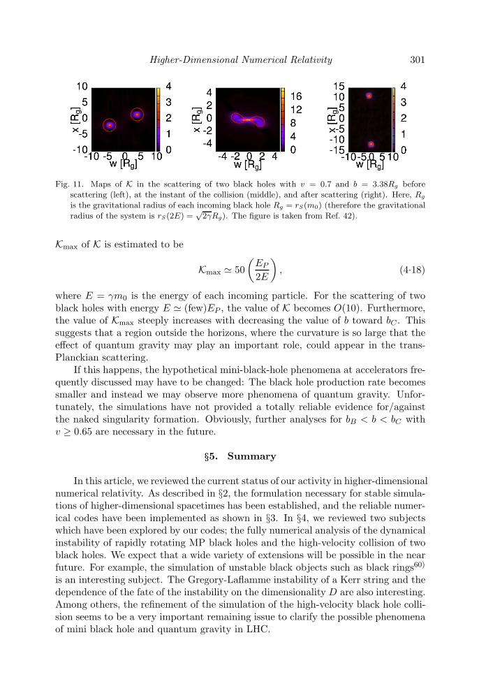
P ) of Kis adopted as the value of |RabcdRabcd|1/2 at the horizon of a black hole with mass EP .Figure 11 displays the maps of K for various stages (before collision, at the instant ofcollision, after collision from left to right) in the scattering process of two black holesfor v = 0.7 and b = 3.38Rg. At the instant of the collision, the curvature invariantK steeply increases around the center of mass, and it subsequently decreases withincreasing the separation of two black holes after the scattering. The maximum value


Fig. 11. Maps of K in the scattering of two black holes with v = 0.7 and b = 3.38Rg before

scattering (left), at the instant of the collision (middle), and after scattering (right). Here, Rg

is the gravitational radius of each incoming black hole Rg = rS(m0) (therefore the gravitational

radius of the system is rS(2E) =√

2γRg). The figure is taken from Ref. 42).

Kmax of K is estimated to be

Kmax � 50(EP

2E

), (4.18)

where E = γm0 is the energy of each incoming particle. For the scattering of twoblack holes with energy E � (few)EP , the value of K becomes O(10). Furthermore,the value of Kmax steeply increases with decreasing the value of b toward bC . Thissuggests that a region outside the horizons, where the curvature is so large that theeffect of quantum gravity may play an important role, could appear in the trans-Planckian scattering.

If this happens, the hypothetical mini-black-hole phenomena at accelerators fre-quently discussed may have to be changed: The black hole production rate becomessmaller and instead we may observe more phenomena of quantum gravity. Unfor-tunately, the simulations have not provided a totally reliable evidence for/againstthe naked singularity formation. Obviously, further analyses for bB < b < bC withv ≥ 0.65 are necessary in the future.

§5. Summary

In this article, we reviewed the current status of our activity in higher-dimensionalnumerical relativity. As described in §2, the formulation necessary for stable simula-tions of higher-dimensional spacetimes has been established, and the reliable numer-ical codes have been implemented as shown in §3. In §4, we reviewed two subjectswhich have been explored by our codes; the fully numerical analysis of the dynamicalinstability of rapidly rotating MP black holes and the high-velocity collision of twoblack holes. We expect that a wide variety of extensions will be possible in the nearfuture. For example, the simulation of unstable black objects such as black rings60)

is an interesting subject. The Gregory-Laflamme instability of a Kerr string and thedependence of the fate of the instability on the dimensionality D are also interesting.Among others, the refinement of the simulation of the high-velocity black hole colli-sion seems to be a very important remaining issue to clarify the possible phenomenaof mini black hole and quantum gravity in LHC.


In §1, we introduced AdS/CFT correspondence as one of the subjects for higher-dimensional numerical relativity. To study the issues of AdS/CFT correspondencein numerical relativity, a formulation to handle the spacetimes with a negativecosmological constant Λ < 0 has to be developed. The formulation for handlingΛ < 0 is also necessary for simulating black hole dynamics in the Randall-Sundrumbraneworld scenarios.

Another interesting direction in the future is to develop formulations and codesfor simulating spacetimes in Gauss-Bonnet gravity62) (or, more generally, Lovelockgravity63)). The Gauss-Bonnet gravity is a theory derived from a Lagrangian densitywith higher-order curvature terms, L = R+αGBLGB and LGB = R2−4RMNR

MN +RKLMNR

KLMN , but is a well-behaved theory in the sense that the 3rd and 4th-orderderivative terms of the metric do not appear in equations. The presence of the Gauss-Bonnet terms is predicted by low-energy limit of heterotic string theory. Becausethe higher-curvature terms may become important in mini black hole productionat accelerators and it causes a lot of interesting phenomena such as instabilities ofspherically symmetric black holes,64) exploring the dynamics of the higher-curvaturetheory will be an interesting subject. The (N + 1)-formalism for Gauss-Bonnetgravity, which corresponds to the ADM formalism in general relativity, was developedby Torii and Shinkai,65) and the first numerical study for the black hole initial datain Gauss-Bonnet gravity was done by Yoshino.66) Further development in this fieldis expected.

References

1) F. Pretorius, Phys. Rev. Lett. 95 (2005), 121101.2) M. Campanelli, C. O. Lousto, P. Marronetti and Y. Zlochower, Phys. Rev. Lett. 96 (2006),

111101.3) J. G. Baker, J. Centrella, D. I. Choi, M. Koppitz and J. van Meter, Phys. Rev. Lett. 96

(2006), 111102.4) P. Diener et al., Phys. Rev. Lett. 96 (2006), 121101.5) F. Herrmann, I. Hinder, D. Shoemaker and P. Laguna, gr-qc/0601026.6) M. Boyle, D. A. Brown, L. E. Kidder, A. H. Mroue, H. P. Pfeiffer, M. A. Scheel, G. B. Cook,

and S. A. Teukolsky, Phys. Rev. D 76 (2007), 124038.7) M. D. Duez, Class. Quant. Grav. 27 (2010), 114002.8) M. Shibata and K. Taniguchi, Living Rev. Rel. (2011), to appear.9) N. Arkani-Hamed, S. Dimopoulos and G. R. Dvali, Phys. Lett. B 429 (1998), 263.

10) I. Antoniadis, N. Arkani-Hamed, S. Dimopoulos and G. R. Dvali, Phys. Lett. B 436 (1998),257.

11) L. Randall and R. Sundrum, Phys. Rev. Lett. 83 (1999), 3370.12) L. Randall and R. Sundrum, Phys. Rev. Lett. 83 (1999), 4690.13) J. M. Maldacena, Adv. Theor. Math. Phys. 2 (1998), 231; Int. J. Theor. Phys. 38 (1999),

1113.14) M. Choptuik, L. Lehner, I. I. Olabarrieta, R. Petryk, F. Pretorius and H. Villegas, Phys.

Rev. D 68 (2003), 044001.15) D. Garfinkle, L. Lehner and F. Pretorius, Phys. Rev. D 71 (2005), 064009.16) T. Banks and W. Fischler, hep-th/9906038.17) S. Dimopoulos and G. Landsberg, Phys. Rev. Lett. 87 (2001), 161602.18) S. B. Giddings and S. Thomas, Phys. Rev. D 65 (2002), 056010.19) P. Kanti, Lect. Notes Phys. 769 (2009), 387.20) H. Yoshino and Y. Nambu, Phys. Rev. D 67 (2003), 024009.21) H. Yoshino and V. S. Rychkov, Phys. Rev. D 71 (2005), 104028.22) P. C. Aichelburg and R. U. Sexl, Gen. Relat. Gravit. 2 (1971), 303.


23) D. M. Eardley and S. B. Giddings, Phys. Rev. D 66 (2002), 044011.24) R. Gregory and R. Laflamme, Phys. Rev. Lett. 70 (1993), 2837.25) R. C. Myers and M. J. Perry, Ann. of Phys. 172 (1986), 304.26) R. Emparan and R. C. Myers, J. High Energy Phys. 09 (2003), 025.27) O. J. C. Dias, P. Figueras, R. Monteiro, J. E. Santos and R. Emparan, Phys. Rev. D 80

(2009), 111701.28) M. Shibata and H. Yoshino, Phys. Rev. D 81 (2010), 021501.29) M. Shibata and H. Yoshino, Phys. Rev. D 81 (2010), 104035.30) H. Yoshino, J. High Energy Phys. 01 (2009), 068.31) H. Yoshino and M. Shibata, Prog. Theor. Phys. Suppl. No. 189 (2011), 269.32) M. Shibata and T. Nakamura, Phys. Rev. D 52 (1995), 5428.33) T. W. Baumgarte and S. L. Shapiro, Phys. Rev. D 59 (1998), 024007.34) H. Yoshino and M. Shibata, Phys. Rev. D 80 (2009), 084025.35) R. Arnowitt, S. Deser and C. W. Misner, in Gravitation: An Introduction to Current

Research, ed. L. Witten (Wiley, 1962), p. 227.36) M. Alcubierre, S. Brandt, B. Brugmann, D. Holz, E. Seidel, R. Takahashi and J. Thorn-

burg, Int. J. Mod. Phys. D 10 (2001), 273.37) I. Novikov, Ph.D. thesis (Shternberg Astronomical Institute, Moscow, 1963).38) C. Misner, K. Thorne, and J. Wheeler, Gravitation (W. H. Freeman and Company, San

Francisco, 1973), p. 826.39) F. Estabrook, H. Wahlquist, S. Christensen, B. DeWitt, L. Smarr and E. Tsiang, Phys.

Rev. D 7 (1973), 2814.40) T. W. Baumgarte and S. G. Naculich, Phys. Rev. D 75 (2007), 067502.41) K. I. Nakao, H. Abe, H. Yoshino and M. Shibata, Phys. Rev. D 80 (2009), 084028.42) H. Okawa, K. i. Nakao, and M. Shibata, arXiv:1105.3331.43) L. Lehner and F. Pretorius, Phys. Rev. Lett. 105 (2010), 101102.44) M. Zilhao, H. Witek, U. Sperhake, V. Cardoso, L. Gualtieri, C. Herdeiro and A. Nerozzi,

Phys. Rev. D 81 (2010), 084052.45) H. Witek, M. Zilhao, L. Gualtieri, V. Cardoso, C. Herdeiro, A. Nerozzi and U. Sperhake,

Phys. Rev. D 82 (2010), 104014.46) H. Witek, V. Cardoso, L. Gualtieri, C. Herdeiro, U. Sperhake and M. Zilhao, Phys. Rev.

D 83 (2011), 044017.47) E. Sorkin, Phys. Rev. D 81 (2010), 084062.48) Y. Yamada and H. Shinkai, Phys. Rev. D 83 (2011), 064006, arXiv:1102.2090.49) T. Oota and Y. Yasui, Int. J. Mod. Phys. A 25 (2010), 3055.50) H. Kodama, R. A. Konoplya and A. Zhidenko, Phys. Rev. D 81 (2010), 044007.51) T. Yamamoto, M. Shibata and K. Taniguchi, Phys. Rev. D 78 (2008), 064054.52) S. A. Teukolsky and W. H. Press, Astrophys. J. 193 (1974), 443.53) U. Sperhake, V. Cardoso, F. Pretorius, E. Berti and J. A. Gonzalez, Phys. Rev. Lett. 101

(2008), 161101.54) M. Shibata, H. Okawa and T. Yamamoto, Phys. Rev. D 78 (2008), 101501(R).55) U. Sperhake, V. Cardoso, F. Pretorius, E. Berti, T. Hinderer and N. Yunes, Phys. Rev.

Lett. 103 (2009), 131102.56) J. M. Bowen and J. W. York, Jr., Phys. Rev. D 21 (1980), 2047.57) S. Brandt and B. Brugmann, Phys. Rev. Lett. 78 (1997), 3606.58) H. Yoshino, T. Shiromizu and M. Shibata, Phys. Rev. D 72 (2005), 084020.59) H. Yoshino, T. Shiromizu and M. Shibata, Phys. Rev. D 74 (2006), 124022.60) R. Emparan and H. S. Reall, Phys. Rev. Lett. 88 (2002), 101101.61) H. Witek, V. Cardoso, C. Herdeiro, A. Nerozzi, U. Sperhake and M. Zilhao, Phys. Rev. D

82 (2010), 104037.62) C. Lanczos, Ann. Math. 39 (1938), 842.63) D. Lovelock, J. Math. Phys. 12 (1971), 498.64) M. Beroiz, G. Dotti and R. J. Gleiser, Phys. Rev. D 76 (2007), 024012.65) T. Torii and H. Shinkai, Phys. Rev. D 78 (2008), 084037.66) H. Yoshino, Phys. Rev. D 83 (2011), 104010.

Exploring Higher-Dimensional Black Holes in Numerical ...masaru.shibata/PTPS190.282.pdf ·...

Documents

Transcript of Exploring Higher-Dimensional Black Holes in Numerical ...masaru.shibata/PTPS190.282.pdf ·...