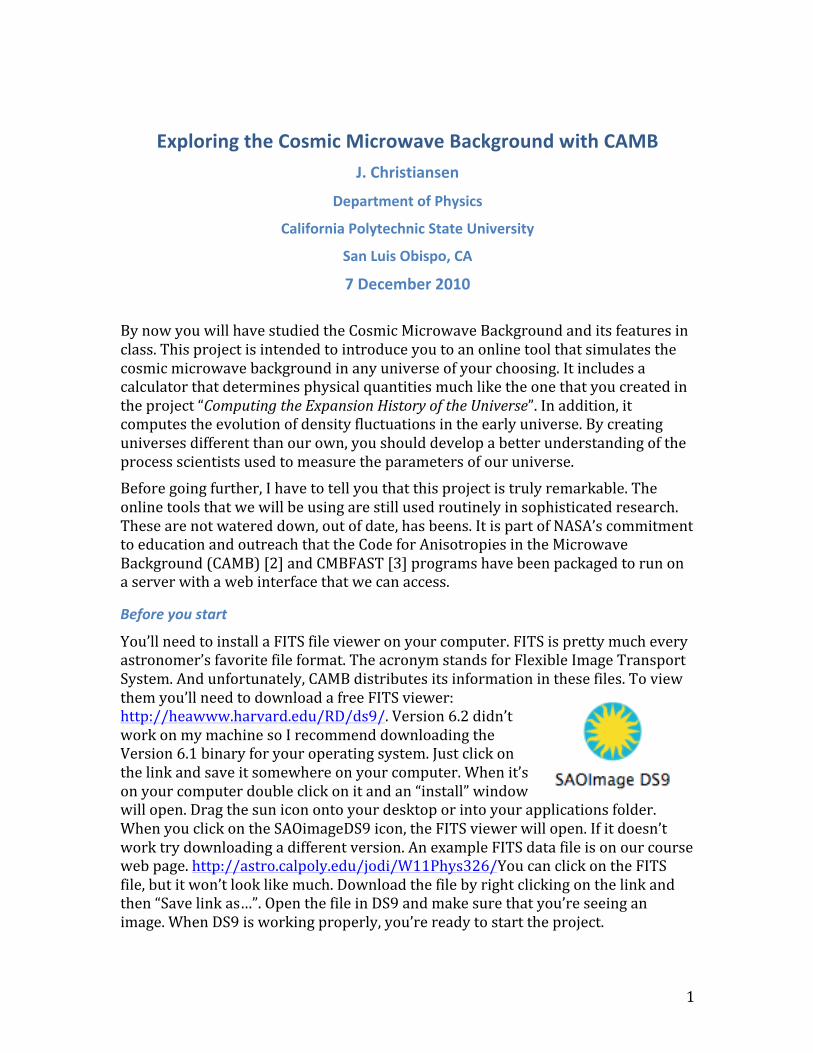
1  

Exploring  the  Cosmic  Microwave  Background  with  CAMB  J.  Christiansen  

Department  of  Physics  

California  Polytechnic  State  University  

San  Luis  Obispo,  CA  

7  December  2010    By  now  you  will  have  studied  the  Cosmic  Microwave  Background  and  its  features  in  class.  This  project  is  intended  to  introduce  you  to  an  online  tool  that  simulates  the  cosmic  microwave  background  in  any  universe  of  your  choosing.  It  includes  a  calculator  that  determines  physical  quantities  much  like  the  one  that  you  created  in  the  project  “Computing  the  Expansion  History  of  the  Universe”.  In  addition,  it  computes  the  evolution  of  density  fluctuations  in  the  early  universe.  By  creating  universes  different  than  our  own,  you  should  develop  a  better  understanding  of  the  process  scientists  used  to  measure  the  parameters  of  our  universe.  Before  going  further,  I  have  to  tell  you  that  this  project  is  truly  remarkable.  The  online  tools  that  we  will  be  using  are  still  used  routinely  in  sophisticated  research.  These  are  not  watered  down,  out  of  date,  has  beens.  It  is  part  of  NASA’s  commitment  to  education  and  outreach  that  the  Code  for  Anisotropies  in  the  Microwave  Background  (CAMB)  [2]  and  CMBFAST  [3]  programs  have  been  packaged  to  run  on  a  server  with  a  web  interface  that  we  can  access.  

Before  you  start  

You’ll  need  to  install  a  FITS  file  viewer  on  your  computer.  FITS  is  pretty  much  every  astronomer’s  favorite  file  format.  The  acronym  stands  for  Flexible  Image  Transport  System.  And  unfortunately,  CAMB  distributes  its  information  in  these  files.  To  view  them  you’ll  need  to  download  a  free  FITS  viewer:  http://heawww.harvard.edu/RD/ds9/.  Version  6.2  didn’t  work  on  my  machine  so  I  recommend  downloading  the  Version  6.1  binary  for  your  operating  system.  Just  click  on  the  link  and  save  it  somewhere  on  your  computer.  When  it’s  on  your  computer  double  click  on  it  and  an  “install”  window  will  open.  Drag  the  sun  icon  onto  your  desktop  or  into  your  applications  folder.  When  you  click  on  the  SAOimageDS9  icon,  the  FITS  viewer  will  open.  If  it  doesn’t  work  try  downloading  a  different  version.  An  example  FITS  data  file  is  on  our  course  web  page.  http://astro.calpoly.edu/jodi/W11Phys326/You  can  click  on  the  FITS  file,  but  it  won’t  look  like  much.  Download  the  file  by  right  clicking  on  the  link  and  then  “Save  link  as…”.  Open  the  file  in  DS9  and  make  sure  that  you’re  seeing  an  image.  When  DS9  is  working  properly,  you’re  ready  to  start  the  project.  

Exploring  the  CMB  with  CAMB  

  2  

Part  1  –  Simulating  CMB  Maps  

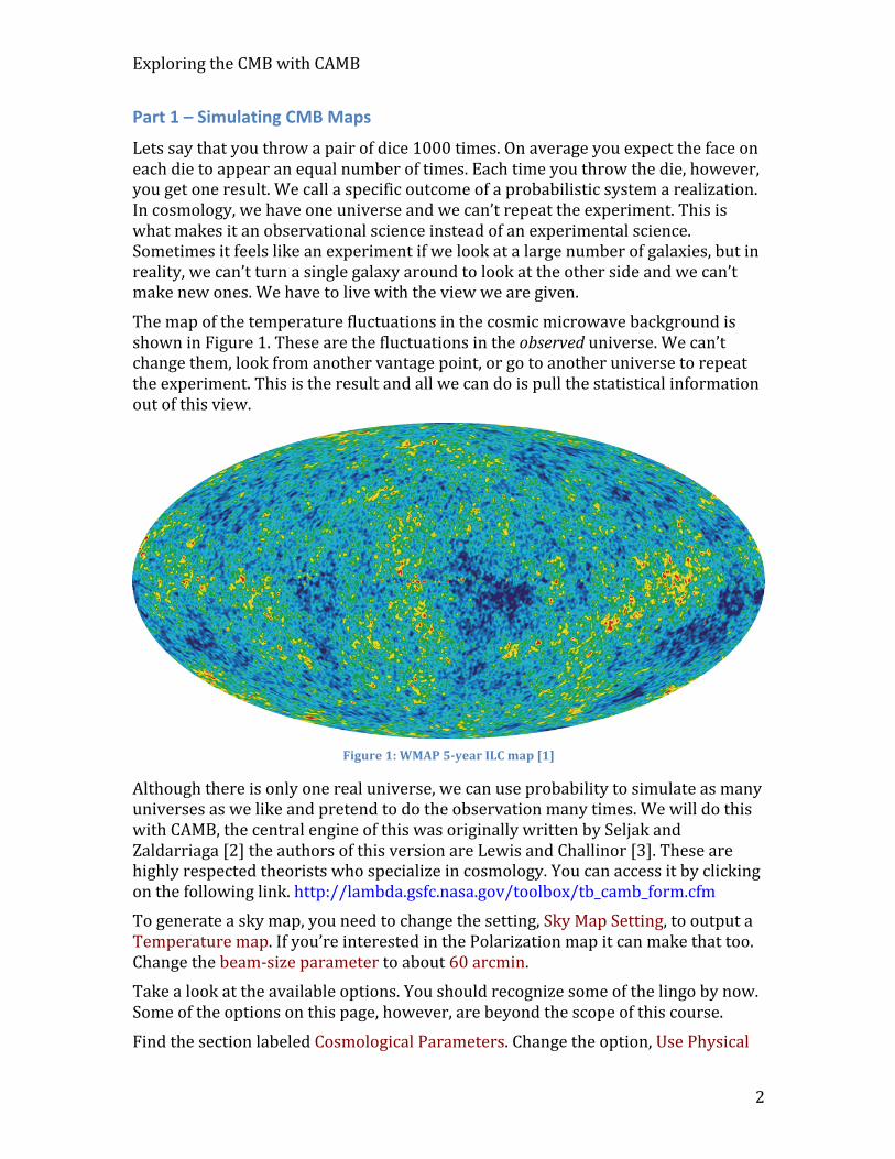
Lets  say  that  you  throw  a  pair  of  dice  1000  times.  On  average  you  expect  the  face  on  each  die  to  appear  an  equal  number  of  times.  Each  time  you  throw  the  die,  however,  you  get  one  result.  We  call  a  specific  outcome  of  a  probabilistic  system  a  realization.  In  cosmology,  we  have  one  universe  and  we  can’t  repeat  the  experiment.  This  is  what  makes  it  an  observational  science  instead  of  an  experimental  science.  Sometimes  it  feels  like  an  experiment  if  we  look  at  a  large  number  of  galaxies,  but  in  reality,  we  can’t  turn  a  single  galaxy  around  to  look  at  the  other  side  and  we  can’t  make  new  ones.  We  have  to  live  with  the  view  we  are  given.    The  map  of  the  temperature  fluctuations  in  the  cosmic  microwave  background  is  shown  in  Figure  1.  These  are  the  fluctuations  in  the  observed  universe.  We  can’t  change  them,  look  from  another  vantage  point,  or  go  to  another  universe  to  repeat  the  experiment.  This  is  the  result  and  all  we  can  do  is  pull  the  statistical  information  out  of  this  view.  

 Figure  1:  WMAP  5-­‐year  ILC  map  [1]  

Although  there  is  only  one  real  universe,  we  can  use  probability  to  simulate  as  many  universes  as  we  like  and  pretend  to  do  the  observation  many  times.  We  will  do  this  with  CAMB,  the  central  engine  of  this  was  originally  written  by  Seljak  and  Zaldarriaga  [2]  the  authors  of  this  version  are  Lewis  and  Challinor  [3].  These  are  highly  respected  theorists  who  specialize  in  cosmology.  You  can  access  it  by  clicking  on  the  following  link.  http://lambda.gsfc.nasa.gov/toolbox/tb_camb_form.cfm  To  generate  a  sky  map,  you  need  to  change  the  setting,  Sky  Map  Setting,  to  output  a  Temperature  map.  If  you’re  interested  in  the  Polarization  map  it  can  make  that  too.  Change  the  beam-­‐size  parameter  to  about  60  arcmin.  Take  a  look  at  the  available  options.  You  should  recognize  some  of  the  lingo  by  now.  Some  of  the  options  on  this  page,  however,  are  beyond  the  scope  of  this  course.  Find  the  section  labeled  Cosmological  Parameters.  Change  the  option,  Use  Physical  

Exploring  the  CMB  with  CAMB  

  3  

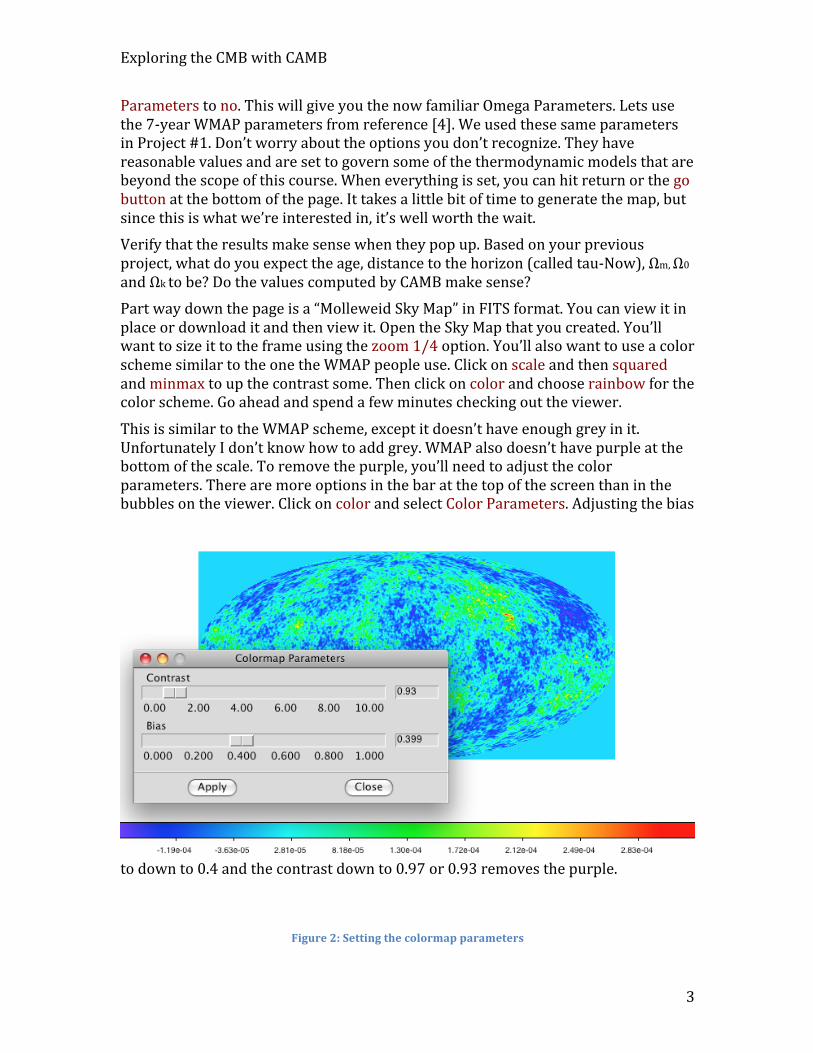
Parameters  to  no.  This  will  give  you  the  now  familiar  Omega  Parameters.  Lets  use  the  7-­‐year  WMAP  parameters  from  reference  [4].  We  used  these  same  parameters  in  Project  #1.  Don’t  worry  about  the  options  you  don’t  recognize.  They  have  reasonable  values  and  are  set  to  govern  some  of  the  thermodynamic  models  that  are  beyond  the  scope  of  this  course.  When  everything  is  set,  you  can  hit  return  or  the  go  button  at  the  bottom  of  the  page.  It  takes  a  little  bit  of  time  to  generate  the  map,  but  since  this  is  what  we’re  interested  in,  it’s  well  worth  the  wait.  Verify  that  the  results  make  sense  when  they  pop  up.  Based  on  your  previous  project,  what  do  you  expect  the  age,  distance  to  the  horizon  (called  tau-­‐Now),  Ωm,  Ω0  and  Ωk  to  be?  Do  the  values  computed  by  CAMB  make  sense?  Part  way  down  the  page  is  a  “Molleweid  Sky  Map”  in  FITS  format.  You  can  view  it  in  place  or  download  it  and  then  view  it.  Open  the  Sky  Map  that  you  created.  You’ll  want  to  size  it  to  the  frame  using  the  zoom  1/4  option.  You’ll  also  want  to  use  a  color  scheme  similar  to  the  one  the  WMAP  people  use.  Click  on  scale  and  then  squared  and  minmax  to  up  the  contrast  some.  Then  click  on  color  and  choose  rainbow  for  the  color  scheme.  Go  ahead  and  spend  a  few  minutes  checking  out  the  viewer.  This  is  similar  to  the  WMAP  scheme,  except  it  doesn’t  have  enough  grey  in  it.  Unfortunately  I  don’t  know  how  to  add  grey.  WMAP  also  doesn’t  have  purple  at  the  bottom  of  the  scale.  To  remove  the  purple,  you’ll  need  to  adjust  the  color  parameters.  There  are  more  options  in  the  bar  at  the  top  of  the  screen  than  in  the  bubbles  on  the  viewer.  Click  on  color  and  select  Color  Parameters.  Adjusting  the  bias  

to  down  to  0.4  and  the  contrast  down  to  0.97  or  0.93  removes  the  purple.      

Figure  2:  Setting  the  colormap  parameters  

Exploring  the  CMB  with  CAMB  

  4  

Report:  Run  the  simulation  4  times  and  include  screen  shots  of  the  images  in  your  report.  Describe  how  the  character  of  the  spots  doesn’t  change  even  though  the  pictures  are  completely  different  from  one  another.  Verify  that  the  CAMB  results  make  sense  based  on  your  previous  project.  Do  the  age,  distance  to  the  horizon  (called  tau-­‐Now),  Ωm,  Ω0,  and  Ωk  agree?  Now  check  out  a  low-­‐density  universe.  Set  Ωcdm  and  ΩLambda  to  zero.  Do  the  spots  look  like  they  did  before?  Comment  on  any  differences  you  observe.  Which  plots  most  closely  resemble  the  observed  WMAP  sky  map  shown  in  Figure  1?  

Part  2  –  Finding  Cosmological  Parameters  from  the  Power  Spectrum  

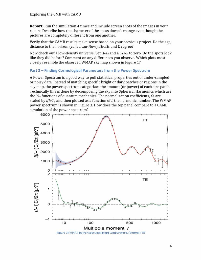
A  Power  Spectrum  is  a  good  way  to  pull  statistical  properties  out  of  under-­‐sampled  or  noisy  data.  Instead  of  matching  specific  bright  or  dark  patches  or  regions  in  the  sky  map,  the  power  spectrum  categorizes  the  amount  (or  power)  of  each  size  patch.  Technically  this  is  done  by  decomposing  the  sky  into  Spherical  Harmonics  which  are  the  Ylm  functions  of  quantum  mechanics.  The  normalization  coefficients,  Cl,  are  scaled  by  l(l+1)  and  then  plotted  as  a  function  of  l,  the  harmonic  number.  The  WMAP  power  spectrum  is  shown  in  Figure  3.  How  does  the  top  panel  compare  to  a  CAMB  simulation  of  the  power  spectrum?  

 Figure  3:  WMAP  power  spectrum  (top)  temperature,  (bottom)  TE  

Exploring  the  CMB  with  CAMB  

  5  

Report:  A. Run  the  program  multiple  times  with  the  same  parameter  settings.  You  have  

seen  that  the  maps  change  every  time  you  run  the  program.  Explain  any  changes  you  observe  in  the  power  spectra  between  different  runs.  Is  the  power  spectrum  insensitive  to  specific  realizations?  

B. Lets  look  at  the  power  spectrum  for  our  favorite  parameter  settings.  Take  a  screen  shot  of  a  sky  map,  and  the  TT  and  TE  power  spectra  to  include  in  your  report.  Record  the  parameters,  age,  and  tau_now  while  you’re  at  it.    

Benchmark  Einstein-­‐deSitter    Low-­‐Density,  Matter-­‐Only    WMAP    

Which  power  spectrum  most  closely  resembles  the  real  WMAP  data?  You’ll  have  to  look  carefully  because  the  CAMB  scale  is  linear  and  the  WMAP  scale  is  logarithmic.  This  can  be  done  with  some  numerical  precision,  however.  

C. To  really  understand  the  sensitivity  of  the  Power  Spectrum,  you  need  to  explore  what  each  Omega  parameter  contributes.  (You  can  turn  off  the  map  making  to  speed  this  part  up.)  

1. Normal  (baryonic)  Matter  Only:  turn  off  all  the  other  parameters.  Slowly  increase  the  baryonic  matter  from  a  small  value  ~0.05  to  a  large  value  like  1.2.  Sketch  the  features  in  the  spectrum  and  how  they  change  as  the  universe  gets  denser.  Describe  the  main  features  that  you  can  attribute  to  matter.  

2. Add  Dark  Matter:  CAMB  won’t  run  unless  there  are  baryons  for  the  photons  to  interact  with.  Set  Omega  matter  to  about  0.05.  Raise  the  dark  matter  contribution  from  0  to  1.2  and  characterize  the  spectrum.  Again,  sketch  the  features  in  the  spectrum  and  how  they  change  as  the  universe  gets  denser  with  dark  matter.  Describe  the  main  features  that  you  can  attribute  to  dark  matter.  

You  should  have  noticed  that  the  primary  peak  moves  to  the  left  as  the  density  goes  up.  The  primary  peak  is  at  l  =  200  in  the  WMAP  data.  How  much  matter  does  it  take  to  move  the  peak  to  l  =  200?  Does  it  matter  if  its  normal  or  dark  matter?  From  your  investigation,  is  there  any  evidence  that  the  universe  contains  dark  matter?  

3. Dark  Energy:  Set  the  baryonic  matter  to  0.05.  Increase  the  dark  energy  from  0  to  about  1.2.  Sketch  and  then  describe  the  features  and  how  they  change  as  dark  energy  is  added.    

4. See  if  you  can  find  a  set  of  parameters  that  is  different  from  the  WMAP  parameters,  but  which  still  does  a  pretty  good  job  of  describing  the  spectrum.  

Please  comment  on  whether  this  exercise  was  helpful  for  understanding  that  the  measurements  are  uniquely  described  by  the  WMAP  parameters,  which  provide  strong  motivation  for  dark  matter  and  dark  energy.  

Exploring  the  CMB  with  CAMB  

  6  

References:  1. WMAP  collaboration,  http://map.gsfc.nasa.gov/news/5yr_release.html  

Downloading  the  5.77  MB  image  will  be  quite  rewarding.  2. U.  Seljak  and  M.  Zaldarriaga,  A  Line-­‐of-­‐Sight  Integration  Approach  to  Cosmic  

Microwave  Background  Anisotropies,  ApJ,  469:  437-­‐444,  (1996).  http://arxiv.org/abs/astro-­‐ph/9603033.  

3. CAMB,  http://camb.info/.  4. WMAP  collaboration,  Seven-­‐Year  Wilkinson  Microwave  Anisotropy  Probe  

Observations:  Sky  Maps,  Systematic  Errors,  and  Basic  Results,  (2011),  ApJS,  192,  14    http://arxiv.org/abs/1001.4744