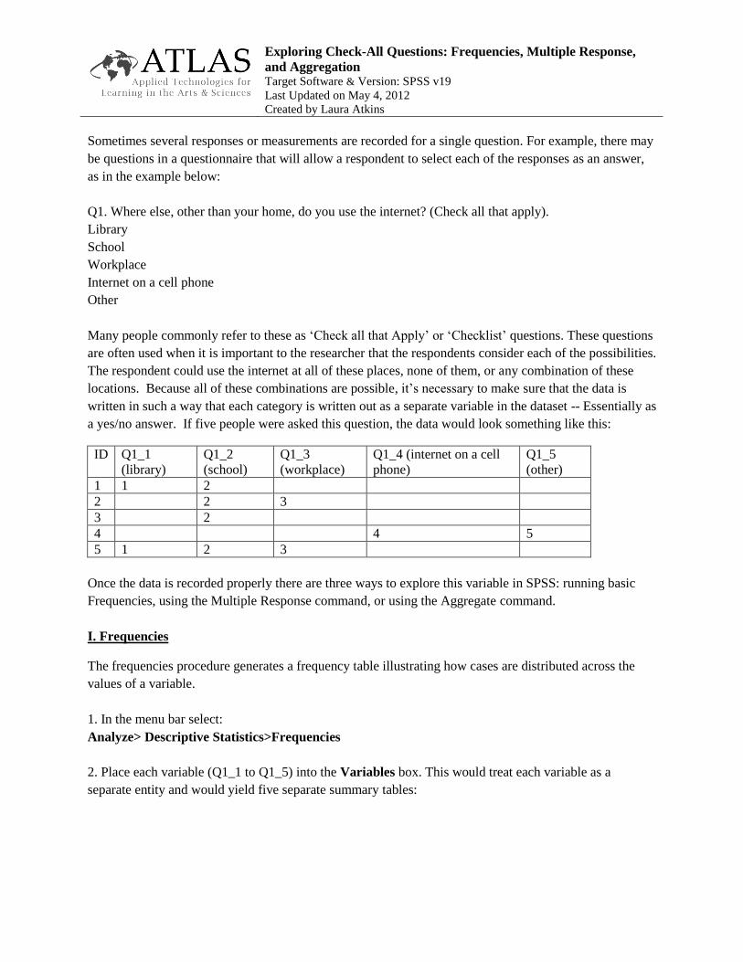
Exploring Check-All Questions: Frequencies, Multiple Response,

and Aggregation Target Software & Version: SPSS v19

Last Updated on May 4, 2012

Created by Laura Atkins

Sometimes several responses or measurements are recorded for a single question. For example, there may

be questions in a questionnaire that will allow a respondent to select each of the responses as an answer,

as in the example below:

Q1. Where else, other than your home, do you use the internet? (Check all that apply).

Library

School

Workplace

Internet on a cell phone

Other

Many people commonly refer to these as ‘Check all that Apply’ or ‘Checklist’ questions. These questions

are often used when it is important to the researcher that the respondents consider each of the possibilities.

The respondent could use the internet at all of these places, none of them, or any combination of these

locations. Because all of these combinations are possible, it’s necessary to make sure that the data is

written in such a way that each category is written out as a separate variable in the dataset -- Essentially as

a yes/no answer. If five people were asked this question, the data would look something like this:

ID Q1_1

(library)

Q1_2

(school)

Q1_3

(workplace)

Q1_4 (internet on a cell

phone)

Q1_5

(other)

1 1 2

2 2 3

3 2

4 4 5

5 1 2 3

Once the data is recorded properly there are three ways to explore this variable in SPSS: running basic

Frequencies, using the Multiple Response command, or using the Aggregate command.

I. Frequencies

The frequencies procedure generates a frequency table illustrating how cases are distributed across the

values of a variable.

1. In the menu bar select:

Analyze> Descriptive Statistics>Frequencies

2. Place each variable (Q1_1 to Q1_5) into the Variables box. This would treat each variable as a

separate entity and would yield five separate summary tables:

II. Multiple Response

A simple, but limited and temporary approach is to use the Multiple Response option. This procedure

creates a single summary table of counts and percents based on several variables that contain responses to

one question. This would create one table that combines all five variables, rather than five separate tables.

1. First, make note of how the variables of interest are coded. For this example there are five categories

(1-5).

2. Next, instruct SPSS that a set of variables represents responses to a single question of interest. In the

menu bar, go to Analyze>Multiple Response>Define Variable Sets. To define a multiple response set in

SPSS we must specify the list of variables that make up the set, the type of coding used, and a name.

3. Using the arrow button, place variables Q1_1 through Q1_5 in the “Variables in Set” box.

4. Click “Categories” and add “1-5” for the range.

5. Give the new collapsed variable a name (ex. Where_Internet). Next, give the variable a label and click

“Add”. Notice that the set name now appears in the Multiple Response Sets list box. The $ prefix

distinguishes the set name from an ordinary SPSS variable name.

6. Click “Close”.

7. Return to Analyze>Multiple Response. You will now see that two options have been activated:

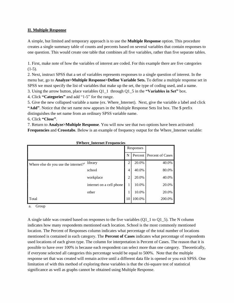
Frequencies and Crosstabs. Below is an example of frequency output for the Where_Internet variable:

$Where_Internet Frequencies

Responses

Percent of Cases N Percent

Where else do you use the internet?a

library 2 20.0% 40.0%

school 4 40.0% 80.0%

workplace 2 20.0% 40.0%

internet on a cell phone 1 10.0% 20.0%

other 1 10.0% 20.0%

Total 10 100.0% 200.0%

a. Group

A single table was created based on responses to the five variables (Q1_1 to Q1_5). The N column

indicates how many respondents mentioned each location. School is the most commonly mentioned

location. The Percent of Responses column indicates what percentage of the total number of locations

mentioned is contained in each category. The Percent of Cases indicates what percentage of respondents

used locations of each given type. The column for interpretation is Percent of Cases. The reason that it is

possible to have over 100% is because each respondent can select more than one category. Theoretically,

if everyone selected all categories this percentage would be equal to 500%. Note that the multiple

response set that was created will remain active until a different data file is opened or you exit SPSS. One

limitation of with this method of exploring these variables is that the chi-square test of statistical

significance as well as graphs cannot be obtained using Multiple Response.

III. Aggregate

A third option for exploring this data is to create a combination variable which would give all of the

unique combinations listed in the dataset. The Aggregate Data command aggregates groups of cases in

the active dataset into single cases and creates a new, aggregated file or creates new variables in the active

dataset that contain aggregated data. Cases are aggregated based on the value of one or more break

(grouping) variables. To do this will take some effort and requires more advanced skills. However, if you

feel that you will be using this variable for statistical tests or beyond a single time period, this could be

the right decision. This option will allow you to save your work and use the variable for later analysis.

The steps are outlined below:

1. Data>Aggregate. Place Q1_1 to Q1_5 in the “Break Variables” box to find unique combinations.

Break Variable(s) are cases which are grouped together based on the values of the break variables. Each

unique combination of break variable values defines a group. When creating a new, aggregated data file,

all break variables are saved in the new file with their existing names and information.

2. Check the “Number of cases” box. This will activate the N_Break command. The N_Break command

tells SPSS by which variable to collapse the data.

3. Check the “Create a new dataset” button and give the new dataset a name. This will specify a new file

into which the aggregated data will be placed. When finished, click OK.

4. In Data View of the new dataset, each row represents a unique response. The cases are represented as

N_Break. Sorting N_break in descending order would show where the most common responses fall.

Additionally, if there were rows with all missing values, these could be deleted because they do not need

to be assigned a unique identifier, which is the next step.

5. To assign a unique identifier to each row, go to: Transform>Compute Variable

Assign a name to the Target Variable (ex.“Values”). In the Function Group box, select “All” and place

$CASENUM into the Numeric Expression box by double-clicking it or using the arrow button.

$Casenum assigns a unique identifier to each row/unique combination of responses.

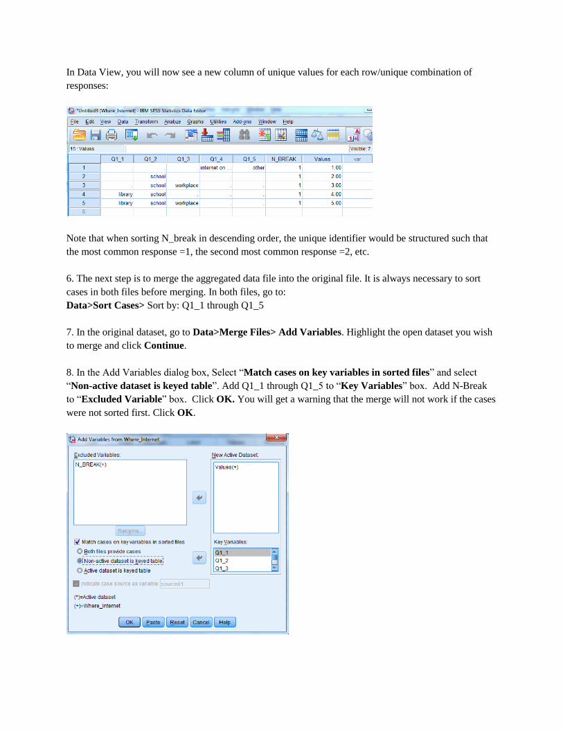
In Data View, you will now see a new column of unique values for each row/unique combination of

responses:

Note that when sorting N_break in descending order, the unique identifier would be structured such that

the most common response =1, the second most common response =2, etc.

6. The next step is to merge the aggregated data file into the original file. It is always necessary to sort

cases in both files before merging. In both files, go to:

Data>Sort Cases> Sort by: Q1_1 through Q1_5

7. In the original dataset, go to Data>Merge Files> Add Variables. Highlight the open dataset you wish

to merge and click Continue.

8. In the Add Variables dialog box, Select “Match cases on key variables in sorted files” and select

“Non-active dataset is keyed table”. Add Q1_1 through Q1_5 to “Key Variables” box. Add N-Break

to “Excluded Variable” box. Click OK. You will get a warning that the merge will not work if the cases

were not sorted first. Click OK.

9. The new variable “Values” can now be seen in Variable View of the original dataset. Change the

decimals to “0”, and add the missing values.

10. The final step is to add values and labels accordingly, by referencing the other data file that shows

unique responses.

Again, the Aggregate command is a useful option if you feel that you will be using the variable for

statistical tests or beyond a single time period. Just save the changes made to your original dataset, and

the new variable will be saved in your dataset.