Exploring Automatic Speech

Recognition with TensorFlow

Degree’s ThesisAudiovisual Systems Engineering

Author: Janna Escur i GelabertAdvisors: Xavier Giro-i-Nieto, Marta Ruiz Costa-Jussa

Universitat Politecnica de Catalunya (UPC)2017 - 2018

Abstract

Speech recognition is the task aiming to identify words in spoken language and convert theminto text. This bachelor’s thesis focuses on using deep learning techniques to build an end-to-endSpeech Recognition system. As a preliminary step, we overview the most relevant methods carriedout over the last several years. Then, we study one of the latest proposals for this end-to-endapproach that uses a sequence to sequence model with attention-based mechanisms. Next, wesuccessfully reproduce the model and test it over the TIMIT database. We analyze the similaritiesand differences between the current implementation proposal and the original theoretical work.And finally, we experiment and contrast using different parameters (e.g. number of layer units,learning rates and batch sizes) and reduce the Phoneme Error Rate in almost 12% relative.

1

Resum

Speech Recognition (reconeixement de veu) es la tasca que preten indentificar paraules delllenguatge parlat i convertir-les a text. Aquest treball de fi de grau es centra en utilitzar tecniquesde deep learning per construir un sistema d’Speech Recognition entrenant-lo end-to-end. Coma pas preliminar, fem un resum dels metodes mes rellevants duts a terme els ultims anys. Acontinuacio, estudiem un dels treballs mes recents en aquesta area que proposa un model se-quence to sequence amb l’atencio entrenat end-to-end. Despres, reproduim satisfactoriamentel model i l’avaluem amb la base de dades TIMIT. Analitzem les semblances i diferencies entrel’implementacio proposada i el treball teoric original. I finalment, experimentem i contrastem elmodel utilitzant diferents parametres (e.g. nombre de neurones per capa, la taxa d’aprenentatge-learning rate- i els batch sizes) i reduim el Phoneme Error Rate gairebe un 12% relatiu.

2

Resumen

Speech Recognition (reconocimiento de voz) es la tarea que pretende indentificar palabrashabladas y convertirlas a texto. Este trabajo de fin de grado se centra en utilizar tecnicas dedeep learning para construir un sistema de Speech Recognition entrenandolo end-to-end. Comopaso preliminar, hacemos un resumen de los metodos mas relevantes llevados a cabo los ultimosanos. A continuacion estudiamos uno de los trabajos mas recientes en este area que proponeun modelo sequence to sequence con atencion entrenado end-to-end. Despues, reproducimossatisfactoriamente el modelo y lo avaluamos con la base de datos TIMIT. Analizamos los parecidosy diferencias entre la implementacion propuesta y el trabajo teorico original. Y finalmente,experimentamos y contrastamos el modelo utilizando diferentes parametros (e.g. numero deneuronas por capa, la tasa de aprendizaje -learning rate y los batch sizes) y reducimos el PhonemeError Rate cerca del 12% relativo.

3

Acknowledgements

First of all, I want to thank my tutor, Xavier Giro-i-Nieto, for making possible my collaborationin this project, and for all his help and efforts from the very beginning. I also want to thankMarta Ruiz for her patience when guiding me and teaching me, and most of all, for helping meevery time I needed.

It has been a pleasure working with Daniel Moreno and Amanda Duarte. I really hopeSpeech2Signs keeps growing and we can continue helping each other.

I am very grateful to Jose Adrian Fonollosa, for providing me the datasets and share to mehis knowledge about speech tasks.

My partners in the X-theses group deserve also a mention here for their ideas and help in thedevelopment of this project.

A special thank to Fran Roldan, for being so passionate about deep learning and helping mein all my doubts.

Finally, I would like to thank Vincent Renkens for his patience and for solving all my issues.Without him this project could not have been carried out.

4

Revision history and approval record

Revision Date Purpose

0 27/12/2017 Document creation

1 24/01/2018 Document revision

2 25/01/2018 Document approbation

DOCUMENT DISTRIBUTION LIST

Name e-mail

Janna Escur janna.escur@alu-etsetb.upc.edu

Xavier Giro i Nieto xavier.giro@upc.edu

Marta Ruiz Costa-Jussa marta.ruiz@upc.edu

Written by: Reviewed and approved by: Reviewed and approved by:

Date 24/01/2018 Date 25/01/2018 Date 25/01/2018

Name Janna Escur NameXavier Giro i Ni-eto

Name Marta Ruiz

Position Project Author PositionProject Supervi-sor

PositionProjectSupervisor

5

Contents

1 Introduction 10

1.1 Motivation . . . . . . . . . . . . . . . . . . . . . . . . . . . . . . . . . . . . . . 10

1.2 Speech to signs . . . . . . . . . . . . . . . . . . . . . . . . . . . . . . . . . . . 10

1.3 Statement of purpose . . . . . . . . . . . . . . . . . . . . . . . . . . . . . . . . 11

1.4 Main Contribution . . . . . . . . . . . . . . . . . . . . . . . . . . . . . . . . . . 11

1.5 Requirements and specifications . . . . . . . . . . . . . . . . . . . . . . . . . . 11

1.6 Methods and procedures . . . . . . . . . . . . . . . . . . . . . . . . . . . . . . 12

1.7 Work Plan . . . . . . . . . . . . . . . . . . . . . . . . . . . . . . . . . . . . . . 12

1.7.1 Work Packages . . . . . . . . . . . . . . . . . . . . . . . . . . . . . . . 12

1.7.2 Gantt Diagram . . . . . . . . . . . . . . . . . . . . . . . . . . . . . . . 13

1.8 Incidents and Modifications . . . . . . . . . . . . . . . . . . . . . . . . . . . . . 13

1.9 Organization . . . . . . . . . . . . . . . . . . . . . . . . . . . . . . . . . . . . . 14

2 State of the art 15

2.1 Hidden Markov Model in Speech Recognition . . . . . . . . . . . . . . . . . . . 15

2.2 Deep Neural Network - Hidden Markov Model (DNN-HMM) . . . . . . . . . . . 16

2.3 End-to-end ASR . . . . . . . . . . . . . . . . . . . . . . . . . . . . . . . . . . . 17

2.3.1 Connectionist Temporal Classification . . . . . . . . . . . . . . . . . . . 17

2.3.2 Sequence to sequence learning with attention mechanism . . . . . . . . . 18

3 Methodology 19

3.1 Baseline . . . . . . . . . . . . . . . . . . . . . . . . . . . . . . . . . . . . . . . 19

3.2 LAS Implementation . . . . . . . . . . . . . . . . . . . . . . . . . . . . . . . . . 21

3.2.1 Differences with respect to the paper . . . . . . . . . . . . . . . . . . . . 21

3.2.2 Kaldi toolkit . . . . . . . . . . . . . . . . . . . . . . . . . . . . . . . . . 22

3.2.3 Configuration files . . . . . . . . . . . . . . . . . . . . . . . . . . . . . . 23

6

3.2.4 Data preparation . . . . . . . . . . . . . . . . . . . . . . . . . . . . . . 23

3.2.5 Training and testing . . . . . . . . . . . . . . . . . . . . . . . . . . . . . 24

3.2.6 Decoding . . . . . . . . . . . . . . . . . . . . . . . . . . . . . . . . . . 24

4 Results 25

4.1 Computational requirements . . . . . . . . . . . . . . . . . . . . . . . . . . . . 25

4.2 Dataset . . . . . . . . . . . . . . . . . . . . . . . . . . . . . . . . . . . . . . . 25

4.3 Evaluation metric . . . . . . . . . . . . . . . . . . . . . . . . . . . . . . . . . . 27

4.4 Experiment analysis . . . . . . . . . . . . . . . . . . . . . . . . . . . . . . . . . 27

5 Budget 31

6 Conclusions 32

7

List of Figures

1.1 Speech2Signs blocks architecture . . . . . . . . . . . . . . . . . . . . . . . . . . 10

1.2 Gantt Diagram of the Degree Thesis . . . . . . . . . . . . . . . . . . . . . . . . 13

2.1 Components of a Speech Recognizer using HMM . . . . . . . . . . . . . . . . . 15

2.2 HMM applied to each phoneme. The output Y is the acoustic vector sequence . 16

2.3 DNN-HMM model structure . . . . . . . . . . . . . . . . . . . . . . . . . . . . 17

3.1 Listen, Attend and Spell model . . . . . . . . . . . . . . . . . . . . . . . . . . . 19

3.2 Listener architecture . . . . . . . . . . . . . . . . . . . . . . . . . . . . . . . . . 20

3.3 Speller architecture . . . . . . . . . . . . . . . . . . . . . . . . . . . . . . . . . 20

3.4 Relation between the configuration files . . . . . . . . . . . . . . . . . . . . . . 23

4.1 Frequency of the phonemes appearance . . . . . . . . . . . . . . . . . . . . . . 28

4.2 Training (left) and validation (right) losses of the model trained with Fisher trainerand Nabu’s parameters . . . . . . . . . . . . . . . . . . . . . . . . . . . . . . . 28

4.3 Training (left) and validation (right) losses of the model trained with Fisher trainerand LAS parameters . . . . . . . . . . . . . . . . . . . . . . . . . . . . . . . . . 29

4.4 Training (left) and validation (right) losses of the model trained with the standardtrainer and Nabu’s parameters . . . . . . . . . . . . . . . . . . . . . . . . . . . 29

4.5 Training (left) and validation (right) losses of the model trained with standardtrainer and LAS parameters . . . . . . . . . . . . . . . . . . . . . . . . . . . . . 30

8

List of Tables

3.1 Differences between Nabu’s implementation and parameters specified in the paper 22

4.1 TIMIT corpus split in train and test sets depending on the dialect region . . . . . 26

4.2 Phoneme error rates of evaluated models . . . . . . . . . . . . . . . . . . . . . . 30

4.3 Reported results on TIMIT Core Test Set . . . . . . . . . . . . . . . . . . . . . 30

5.1 Budget of the project . . . . . . . . . . . . . . . . . . . . . . . . . . . . . . . . 31

9

Chapter 1

Introduction

1.1 Motivation

1.2 Speech to signs

The motivation of training an end-to-end system for Speech Recognition is the project Speech2Signsat UPC, awarded with a Facebook Caffe2 grant, which aims to synthesize a sign language inter-preter from speech.

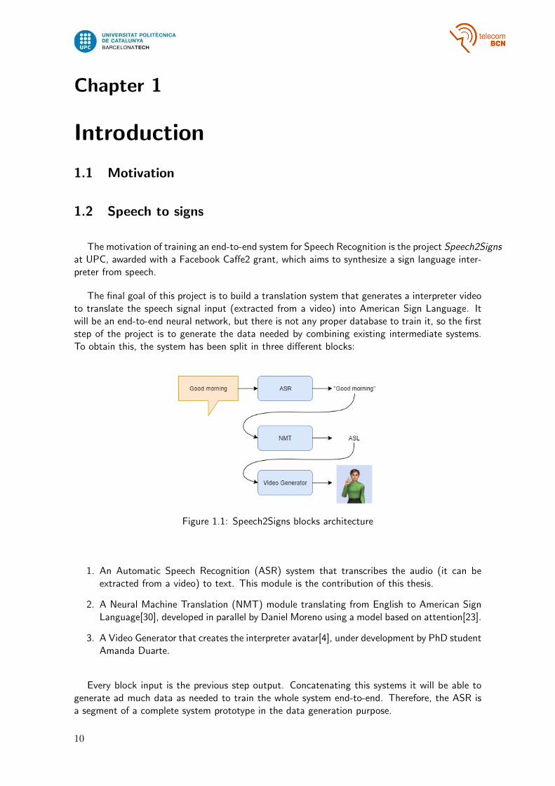
The final goal of this project is to build a translation system that generates a interpreter videoto translate the speech signal input (extracted from a video) into American Sign Language. Itwill be an end-to-end neural network, but there is not any proper database to train it, so the firststep of the project is to generate the data needed by combining existing intermediate systems.To obtain this, the system has been split in three different blocks:

Figure 1.1: Speech2Signs blocks architecture

1. An Automatic Speech Recognition (ASR) system that transcribes the audio (it can beextracted from a video) to text. This module is the contribution of this thesis.

2. A Neural Machine Translation (NMT) module translating from English to American SignLanguage[30], developed in parallel by Daniel Moreno using a model based on attention[23].

3. A Video Generator that creates the interpreter avatar[4], under development by PhD studentAmanda Duarte.

Every block input is the previous step output. Concatenating this systems it will be able togenerate ad much data as needed to train the whole system end-to-end. Therefore, the ASR isa segment of a complete system prototype in the data generation purpose.

10

1.3 Statement of purpose

Speech recognition is the ability of a device or program to identify words in spoken languageand convert them into text. The most frequent applications of speech recognition include speech-to-text processing, voice dialing and voice search. Even if some of these applications work properlyfor the consumer, there is still a room for improvement: sometimes it is hard to recognize thespeech due to variations of pronunciation, it is not well performed for most languages beyondEnglish, and it is necessary to keep fighting against background noise. All these factors can leadto inaccuracies and that is why it is still an interesting research area.

Over the last several years, the number of research projects related to Machine Learninghas increased exponentially, both in the academic and industrial worlds. Such growth has beenboosted by the success of deep learning models in tasks that were considered especially challeng-ing, such as computer vision or natural language processing. Solutions have been found to manytasks obtaining outstanding performances, leading to more complex tasks derived from theseones. Speech recognition is not an exception, even though in the beginning other models wereused (Hidden Markov Models)[13]. Over the years, HMM have been combined with Deep NeuralNetworks and it led to improvements in various components of speech recognition. However, itwas necessary to train different models separately (acoustic, pronunciation and language models).

Recent work in this area attempts to rectify this disjoint training issue by designing modelsthat are trained end-to-end: from speech directly to transcripts. In my work I will focus onsequence to sequence models with attention trained end-to-end[7].

1.4 Main Contribution

This degree’s thesis is developed in the broader context of the Speech2Signs, a project atUPC funded by Facebook, in which a module of Speech Recognition is required. The maincontributions of this thesis is providing a speech recognition system trained end-to-end availablefor integration. This thesis has been written thinking that could be used for other students ordevelopers in the future to participate in upcoming challenges1.

1.5 Requirements and specifications

The requirements of this project are the following:

• Understand Listen, Attend and Spell (LAS) model [6], a deep-learning architecture thatlearns to transcribe speech utterances to characters. It was submitted on 2015 by WilliamChan, Navdeep Jaitly, Quoc V. Le and Oriol Vinyals.

• As it is very challenging to build from scratch a whole system for Speech Recognition, findthe implementation that better achieves the system described on this paper.

• Be able to train the model so it could be used in the Speech2Signs project

1The project can be found in imatge-upc Github: https://github.com/imatge-upc/speech-2018-janna

11

• Have the first deep Speech Recognition model trained end-to-end at GPI and TALP groupsof UPC.

The specifications are the following:

• Use Python as a programming language

• Develop the project using the Tensorflow framework for deep learning

• Use Tensorboard to visualize the results

1.6 Methods and procedures

No deep learning model for speech recognition had been trained end-to-end by the students orresearch groups in the UPC before. In order to do that, it was necessary to find an implementa-tion, and we found Nabu[26], an Automatic Speech Recognizer (ASR) framework for end-to-endnetworks built on Tensorflow, implementing Listen, Attend and Spell paper.

1.7 Work Plan

This project has been developed as a joint effort between the GPI and the TALP researchgroups at Universitat Politecnica de Catalunya, having a regular weekly meeting to discuss de-cisions to be made. This meeting has been complemented with a weekly seminar with otherstudents developing their bachelor, master or Phd thesis at GPI to present our research and shareour knowledge.

The work plan is described in the following work packages and Gantt diagram, as well as themodifications introduced since the first version.

1.7.1 Work Packages

• WP 1: Project management.

• WP 2: Introduction to ASR tasks and TensorFlow

• WP 3: Critical Review of the project

• WP 4: Software development

• WP 6: Dissemination

12

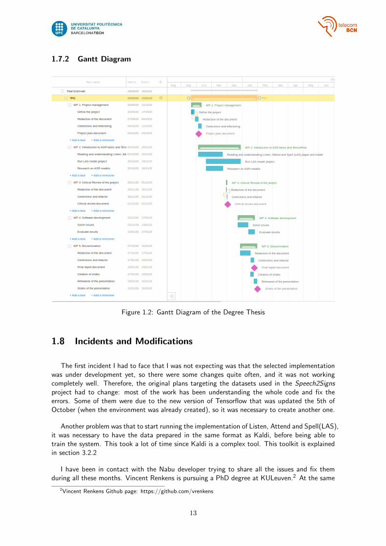
1.7.2 Gantt Diagram

Figure 1.2: Gantt Diagram of the Degree Thesis

1.8 Incidents and Modifications

The first incident I had to face that I was not expecting was that the selected implementationwas under development yet, so there were some changes quite often, and it was not workingcompletely well. Therefore, the original plans targeting the datasets used in the Speech2Signsproject had to change: most of the work has been understanding the whole code and fix theerrors. Some of them were due to the new version of Tensorflow that was updated the 5th ofOctober (when the environment was already created), so it was necessary to create another one.

Another problem was that to start running the implementation of Listen, Attend and Spell(LAS),it was necessary to have the data prepared in the same format as Kaldi, before being able totrain the system. This took a lot of time since Kaldi is a complex tool. This toolkit is explainedin section 3.2.2

I have been in contact with the Nabu developer trying to share all the issues and fix themduring all these months. Vincent Renkens is pursuing a PhD degree at KULeuven.2 At the same

2Vincent Renkens Github page: https://github.com/vrenkens

13

time, working with the whole team of Speech2Signs project, we have been searching datasetsfrom speech to sign language but it has been challenging. We finally end up deciding to splitthe whole project into modules and the train all the separated parts (speech recognition modelis one of them).

Due to the mentioned difficulties in the previous section, running the model took more timethan expected. That is why the phase of testing on other datasets has not been accomplished,and the task became understanding the whole code to be able to solve the issues. But it hasbeen motivating and enriching to have been working in a project under development, gettingdeep into the code and understanding how it really works to be able to solve the errors.

1.9 Organization

The following chapters include a description of the background information related to speechrecognition (Chapter 2), the methodology followed, including the baseline and the description ofimplementation used, as well as the toolkits needed (Chapter3), the results obtained (Chapter4),approximated cost of the project (Chapter5), and finally the conclusions and possible futuredevelopment (Chapter6).

14

Chapter 2

State of the art

Automatic speech recognition (ASR), which identify words in spoken language and convertthem into text, has many potential applications including command and control, dictation, tran-scription of recorded speech, searching audio documents and interactive spoken dialogues. Thischapter presents an overview of the main different approaches to speech recognition.

2.1 Hidden Markov Model in Speech Recognition

Historically, most speech recognition systems have been based on a set of statistical modelsrepresenting the various sounds of the language to be recognized. The hidden Markov model(HMM) is a good framework for constructing such models because speech has temporal structureand can be encoded as a sequence of spectral vectors inside the audio frequency range [13].

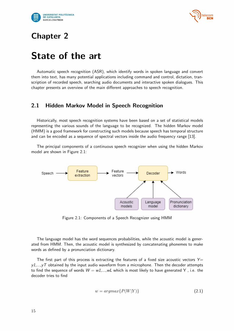
The principal components of a continuous speech recognizer when using the hidden Markovmodel are shown in Figure 2.1:

Figure 2.1: Components of a Speech Recognizer using HMM

The language model has the word sequences probabilities, while the acoustic model is gener-ated from HMM. Then, the acoustic model is synthesized by concatenating phonemes to makewords as defined by a pronunciation dictionary.

The first part of this process is extracting the features of a fixed size acoustic vectors Y=y1,...,yT obtained by the input audio waveform from a microphone. Then the decoder attemptsto find the sequence of words W = w1,...,wL which is most likely to have generated Y , i.e. thedecoder tries to find

w = argmax{P (W |Y )} (2.1)

15

It is used the Bayes’ Rule since P(W/Y) is difficult to model directly, so the previous step itis transformed into the equivalent problem of finding:

w = argmax{P (Y |W )P (W )} (2.2)

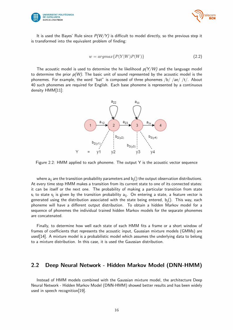
The acoustic model is used to determine the he likelihood p(Y/W) and the language modelto determine the prior p(W). The basic unit of sound represented by the acoustic model is thephonemes. For example, the word “bat” is composed of three phonemes /b/ /ae/ /t/. About40 such phonemes are required for English. Each base phoneme is represented by a continuousdensity HMM[11]:

Figure 2.2: HMM applied to each phoneme. The output Y is the acoustic vector sequence

where aij are the transition probability parameters and bj() the output observation distributions.At every time step HMM makes a transition from its current state to one of its connected states:it can be itself or the next one. The probability of making a particular transition from statesi to state sj is given by the transition probability aij. On entering a state, a feature vector isgenerated using the distribution associated with the state being entered, bj(). This way, eachphoneme will have a different output distribution. To obtain a hidden Markov model for asequence of phonemes the individual trained hidden Markov models for the separate phonemesare concatenated.

Finally, to determine how well each state of each HMM fits a frame or a short window offrames of coefficients that represents the acoustic input, Gaussian mixture models (GMMs) areused[14]. A mixture model is a probabilistic model which assumes the underlying data to belongto a mixture distribution. In this case, it is used the Gaussian distribution.

2.2 Deep Neural Network - Hidden Markov Model (DNN-HMM)

Instead of HMM models combined with the Gaussian mixture model, the architecture DeepNeural Network - Hidden Markov Model (DNN-HMM) showed better results and has been widelyused in speech recognition[19].

16

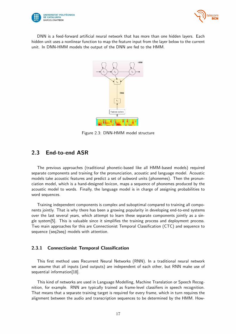
DNN is a feed-forward artificial neural network that has more than one hidden layers. Eachhidden unit uses a nonlinear function to map the feature input from the layer below to the currentunit. In DNN-HMM models the output of the DNN are fed to the HMM.

Figure 2.3: DNN-HMM model structure

2.3 End-to-end ASR

The previous approaches (traditional phonetic-based like all HMM-based models) requiredseparate components and training for the pronunciation, acoustic and language model. Acousticmodels take acoustic features and predict a set of subword units (phonemes). Then the pronun-ciation model, which is a hand-designed lexicon, maps a sequence of phonemes produced by theacoustic model to words. Finally, the language model is in charge of assigning probabilities toword sequences.

Training independent components is complex and suboptimal compared to training all compo-nents jointly. That is why there has been a growing popularity in developing end-to-end systemsover the last several years, which attempt to learn these separate components jointly as a sin-gle system[5]. This is valuable since it simplifies the training process and deployment process.Two main approaches for this are Connectionist Temporal Classification (CTC) and sequence tosequence (seq2seq) models with attention.

2.3.1 Connectionist Temporal Classification

This first method uses Recurrent Neural Networks (RNN). In a traditional neural networkwe assume that all inputs (and outputs) are independent of each other, but RNN make use ofsequential information[18].

This kind of networks are used in Language Modelling, Machine Translation or Speech Recog-nition, for example. RNN are typically trained as frame-level classifiers in speech recognition.That means that a separate training target is required for every frame, which in turn requires thealignment between the audio and transcription sequences to be determined by the HMM. How-

17

ever, the alignments are irrelevant to most speech recognition tasks, where only the word-leveltranscriptions matter. Connectionist Temporal Classification (CTC) is a function that allows anRNN to be trained for sequence transcription tasks without requiring any prior alignment betweenthe input and target sequences[15]. Using CTC, the output layer of the RNN contains a singleunit for each of the transcription labels (characters, phonemes etc.), plus an extra unit referredto as the ‘blank’ which corresponds to a null emission.

For a given transcription sequence, there are as many possible alignments as there differentways of separating the labels with blanks. If using ’/’ to denote blanks, the alignments (/, a, /,b, c, /) and (a, /, b, /, /, c) both correspond to the same transcription (a, b, c). Also, when thesame label appears on successive time-steps in an alignment, the repeats are removed: therefore(a, b, b, b, c, c) and (a, /, b, /, c, c) also correspond to (a, b, c). Intuitively the network decideswhether to emit any label, or no label, at every timestep. Considering these decisions togetherdefine a distribution over alignments between the input and target sequences[16]. CTC then usesa forward-backward algorithm to sum over all possible alignments and determine the normalizedprobability of the target sequence given the input sequence.

CTC assumes that the label outputs are conditionally independent from each others. Jointly,the RNN-CTC model learns the pronunciation and acoustic model together, however it is inca-pable of learning the language model due to conditional independence assumptions similar to aHMM.

2.3.2 Sequence to sequence learning with attention mechanism

Attention Mechanisms in Neural Networks are based on the visual attention mechanism foundin humans. Human visual attention models focus on a certain region of an image with “highresolution” while perceiving the surrounding image in “low resolution”, and then adjusting thefocal point over time. This visual attention can be applied also to speech recognition models.

Unlike CTC-based models, attention-based models do not have conditional-independence as-sumptions and can learn all the components of a speech recognizer including the pronunciation,acoustic and language model directly

• Sequence to sequence learning

Attempts to address the problem of learning variable-length input and output sequencesusing an encoder RNN to map the sequential variable-length input into a fixed-length vector.A decoder RNN then uses this vector to produce the variable-length output sequence.

• Attention mechanism

Sequence to sequence models can be improved by the use of an attention mechanism thatprovides the decoder RNN more information when it produces the output[8][9]. At eachoutput step, the last hidden state of the decoder RNN is used to generate an attentionvector over the input sequence of the encoder. The attention vector is used to propagateinformation from the encoder (which encodes the input sequence to an internal represen-tation) to the decoder (which generate the output sequence) at every time step, insteadof just once, as with the original sequence to sequence model.

18

Chapter 3

Methodology

This chapter presents the methodology used to develop this project and the process followedto be able to get our final results.

3.1 Baseline

The TALP group of UPC had never trained before an end-to-end speech recognition systemas it is quite new. We found it interesting to have a model trained end-to-end that could beused in the future, and the one proposed in ”Listen, Attend and Spell” (LAS) paper[6] was apopular approach in speech recognition community during the last years. This system combines aseq2seq model with an attention mechanism, but it had never been applied to speech recognitionbefore. Very recently(January 2018), new approaches have been proposed, exploring a varietyof structural and optimization improvements to the LAS model, which significantly improveperformance[7].

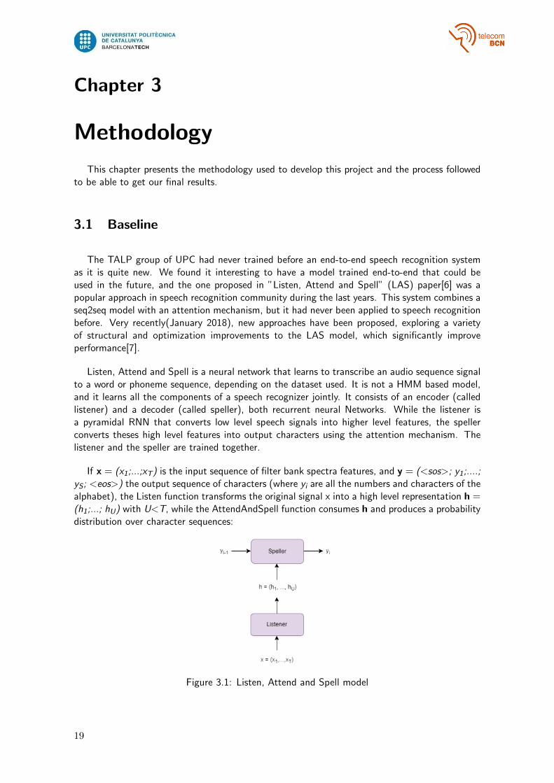
Listen, Attend and Spell is a neural network that learns to transcribe an audio sequence signalto a word or phoneme sequence, depending on the dataset used. It is not a HMM based model,and it learns all the components of a speech recognizer jointly. It consists of an encoder (calledlistener) and a decoder (called speller), both recurrent neural Networks. While the listener isa pyramidal RNN that converts low level speech signals into higher level features, the spellerconverts theses high level features into output characters using the attention mechanism. Thelistener and the speller are trained together.

If x = (x1;...;xT) is the input sequence of filter bank spectra features, and y = (<sos>; y1;....;yS; <eos>) the output sequence of characters (where yi are all the numbers and characters of thealphabet), the Listen function transforms the original signal x into a high level representation h =(h1;...; hU) with U<T, while the AttendAndSpell function consumes h and produces a probabilitydistribution over character sequences:

Figure 3.1: Listen, Attend and Spell model

19

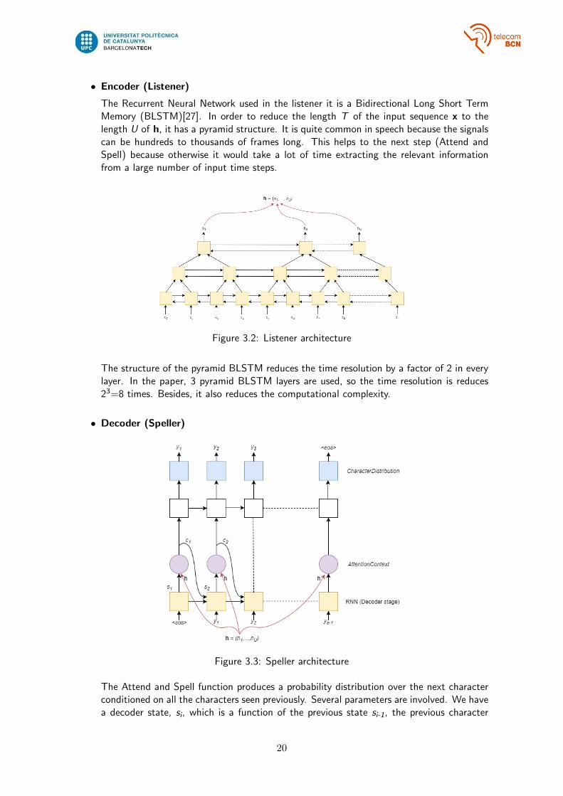
• Encoder (Listener)

The Recurrent Neural Network used in the listener it is a Bidirectional Long Short TermMemory (BLSTM)[27]. In order to reduce the length T of the input sequence x to thelength U of h, it has a pyramid structure. It is quite common in speech because the signalscan be hundreds to thousands of frames long. This helps to the next step (Attend andSpell) because otherwise it would take a lot of time extracting the relevant informationfrom a large number of input time steps.

Figure 3.2: Listener architecture

The structure of the pyramid BLSTM reduces the time resolution by a factor of 2 in everylayer. In the paper, 3 pyramid BLSTM layers are used, so the time resolution is reduces23=8 times. Besides, it also reduces the computational complexity.

• Decoder (Speller)

Figure 3.3: Speller architecture

The Attend and Spell function produces a probability distribution over the next characterconditioned on all the characters seen previously. Several parameters are involved. We havea decoder state, si, which is a function of the previous state si-1, the previous character

20

emitted yi-1 and the previous context vector generated by the attention mechanism, ci-1.The decoder stage is a RNN with 2 layer LSTM.

si = RNN(si-1, yi-1, ci-1) (3.1)

The mentioned context vector ci encapsulates the information in the acoustic signal neededto generate the next character, and it is a function of si and h. To create the context vectorci it is necessary to compute the scalar energy for each time step u using vector hu and si,convert it into a probability distribution over time steps using softmax function and thenlinearly blend the listener features hu at different time steps.

ci = AttentionContext(si,h) (3.2)

A multilayer perceptron with softmax outputs over characters produces the probabilitydistribution.

P (yi|x, y<i) = CharacterDistribution(si, ci) (3.3)

3.2 LAS Implementation

The implementation of LAS network was not provided by the authors, and it was challengingto find one, although we finally succeed. Nabu [26] is an Automatic Speech Recognizer frame-work for end-to-end networks built on TensorFlow[1]. It was still under-development during thedevelopment of this thesis, so it was even more challenging. It works in different stages. First ofall the data preparation is needed, then we can train the model and finally test it. At every stepthere are some configuration files specifying the parameters of the neural network.

3.2.1 Differences with respect to the paper

There are some differences between the model raised in the LAS paper explained in 3.1 and theimplementation of Nabu. Some of them are related to the model and others to the parametersused to train it.

The original paper specifies that 3 layers of 256 nodes per direction are used in the encoder(Listener), but in the Nabu implementation there are 2 layers of 128 units in each layer. There isalso another non-pyramidal layer added during training.The number of timesteps to concatenatein each pyramidal level is 2 in both cases.

The dropout it is not specifically defined in the paper, in the implementation it is 0.5. Thistechnique randomly selects neurons that are ignored during training[29]. They are “dropped-out” randomly. This means that their contribution to the activation of downstream neurons istemporally removed on the forward pass and any weight updates are not applied to the neuronon the backward pass. It is also added a Gaussian input noise during training, and its standarddeviation is set to 0.6.

21

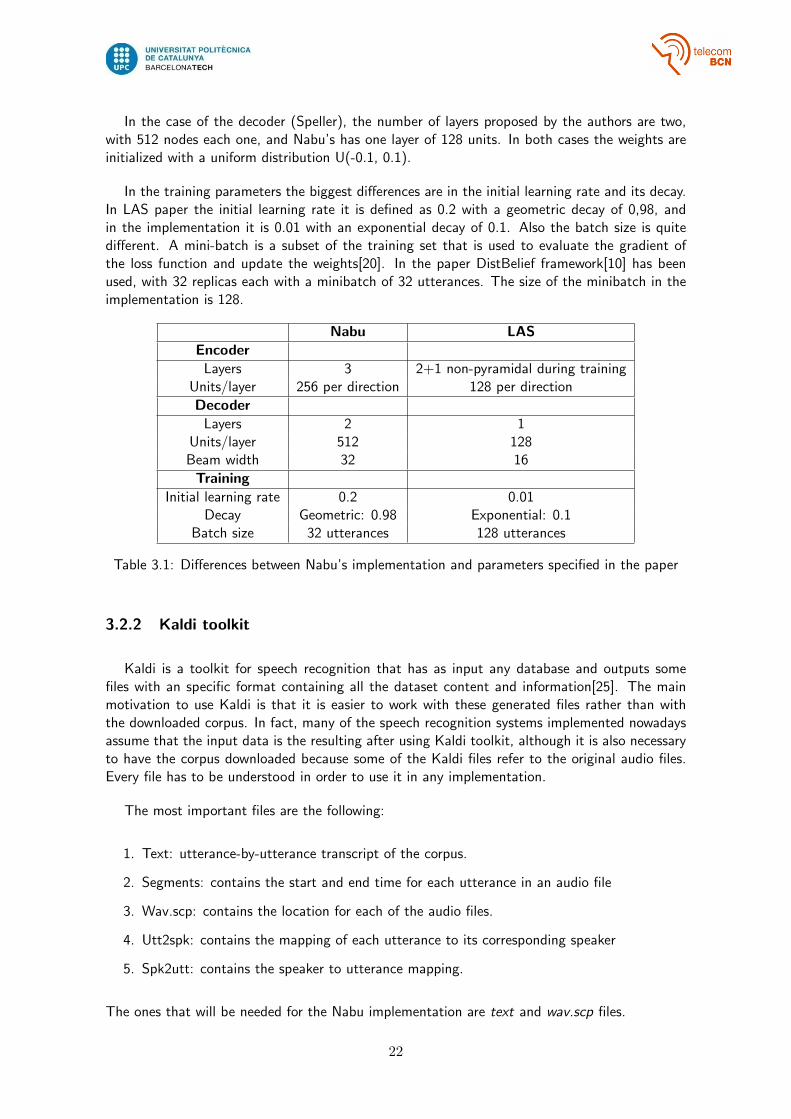
In the case of the decoder (Speller), the number of layers proposed by the authors are two,with 512 nodes each one, and Nabu’s has one layer of 128 units. In both cases the weights areinitialized with a uniform distribution U(-0.1, 0.1).

In the training parameters the biggest differences are in the initial learning rate and its decay.In LAS paper the initial learning rate it is defined as 0.2 with a geometric decay of 0,98, andin the implementation it is 0.01 with an exponential decay of 0.1. Also the batch size is quitedifferent. A mini-batch is a subset of the training set that is used to evaluate the gradient ofthe loss function and update the weights[20]. In the paper DistBelief framework[10] has beenused, with 32 replicas each with a minibatch of 32 utterances. The size of the minibatch in theimplementation is 128.

Nabu LASEncoder

Layers 3 2+1 non-pyramidal during trainingUnits/layer 256 per direction 128 per direction

DecoderLayers 2 1

Units/layer 512 128Beam width 32 16

TrainingInitial learning rate 0.2 0.01

Decay Geometric: 0.98 Exponential: 0.1Batch size 32 utterances 128 utterances

Table 3.1: Differences between Nabu’s implementation and parameters specified in the paper

3.2.2 Kaldi toolkit

Kaldi is a toolkit for speech recognition that has as input any database and outputs somefiles with an specific format containing all the dataset content and information[25]. The mainmotivation to use Kaldi is that it is easier to work with these generated files rather than withthe downloaded corpus. In fact, many of the speech recognition systems implemented nowadaysassume that the input data is the resulting after using Kaldi toolkit, although it is also necessaryto have the corpus downloaded because some of the Kaldi files refer to the original audio files.Every file has to be understood in order to use it in any implementation.

The most important files are the following:

1. Text: utterance-by-utterance transcript of the corpus.

2. Segments: contains the start and end time for each utterance in an audio file

3. Wav.scp: contains the location for each of the audio files.

4. Utt2spk: contains the mapping of each utterance to its corresponding speaker

5. Spk2utt: contains the speaker to utterance mapping.

The ones that will be needed for the Nabu implementation are text and wav.scp files.

22

3.2.3 Configuration files

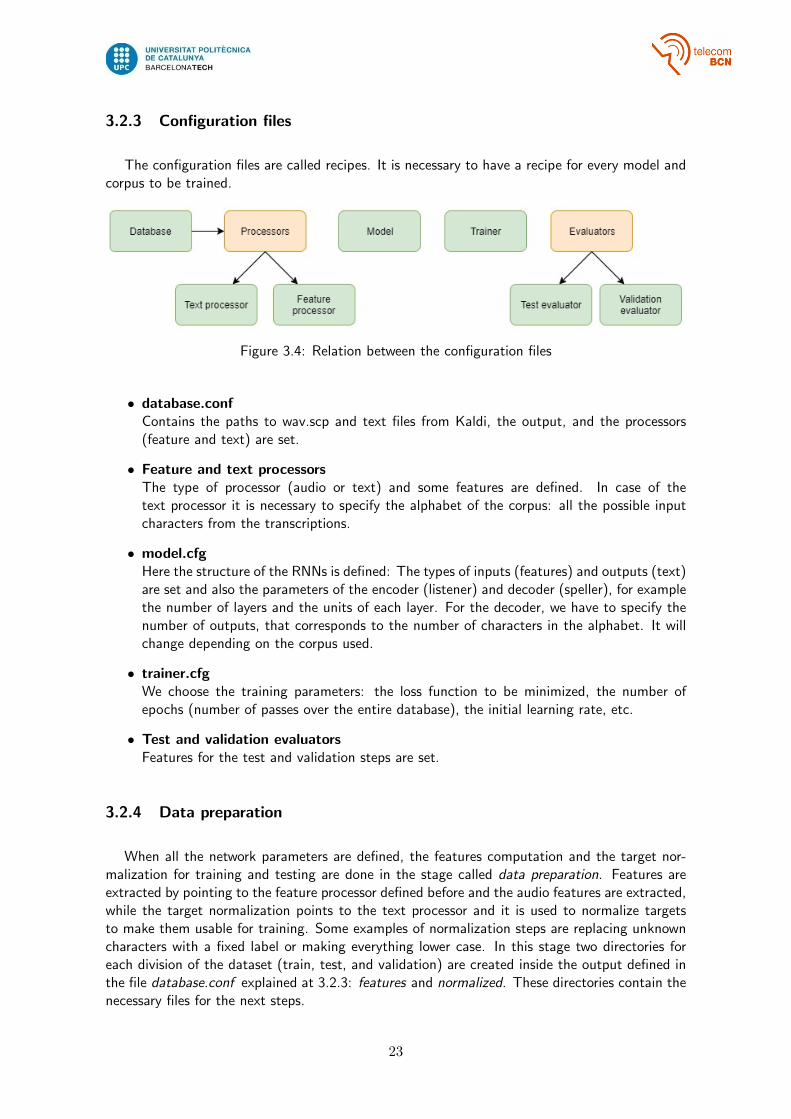
The configuration files are called recipes. It is necessary to have a recipe for every model andcorpus to be trained.

Figure 3.4: Relation between the configuration files

• database.confContains the paths to wav.scp and text files from Kaldi, the output, and the processors(feature and text) are set.

• Feature and text processorsThe type of processor (audio or text) and some features are defined. In case of thetext processor it is necessary to specify the alphabet of the corpus: all the possible inputcharacters from the transcriptions.

• model.cfgHere the structure of the RNNs is defined: The types of inputs (features) and outputs (text)are set and also the parameters of the encoder (listener) and decoder (speller), for examplethe number of layers and the units of each layer. For the decoder, we have to specify thenumber of outputs, that corresponds to the number of characters in the alphabet. It willchange depending on the corpus used.

• trainer.cfgWe choose the training parameters: the loss function to be minimized, the number ofepochs (number of passes over the entire database), the initial learning rate, etc.

• Test and validation evaluatorsFeatures for the test and validation steps are set.

3.2.4 Data preparation

When all the network parameters are defined, the features computation and the target nor-malization for training and testing are done in the stage called data preparation. Features areextracted by pointing to the feature processor defined before and the audio features are extracted,while the target normalization points to the text processor and it is used to normalize targetsto make them usable for training. Some examples of normalization steps are replacing unknowncharacters with a fixed label or making everything lower case. In this stage two directories foreach division of the dataset (train, test, and validation) are created inside the output defined inthe file database.conf explained at 3.2.3: features and normalized. These directories contain thenecessary files for the next steps.

23

3.2.5 Training and testing

In the training step, the model is trained to minimize a loss function (defined in trainer.cfg).During the training, the model can be evaluated using the validation evaluation file to adjust thelearning rate if necessary. Then, we can run the model with the test subset of data, and obtainthe percentage of incorrect characters.

3.2.6 Decoding

In the decoding stage, the model is used to decode the test set and we can see the resultingbest results written in the output. Although the error it is obtained in the test stage, it can beuseful to have both ground truth transcriptions and the output ones if we want to use anothermetric.

24

Chapter 4

Results

This chapter presents the results obtained with the implementation presented in Chapter 3.

4.1 Computational requirements

Experiments have been run with the computational resources available at the Image ProcessingGroup of the Universitat Politecnica de Catalunya. When dealing with deep learning projects,one of the main concerns is the available computation resources, as you are often working withlarge datasets. This is why GPI has a cluster of servers which is shared between all the researchgroup and in which we ran our experiments. For each experiment, we must ask for the resourcesneeded (number of GPU’s/CPU’s, reserve RAM) and the task is sent to a queue of processes.As soon as there is enough resources as you demanded, your process start running. The internalpolicy of GPI allows one GPU per BCs student. It was also needed to access to the VEU serverin order to obtain the datasets.

4.2 Dataset

After realizing that the Nabu implementation was under development and a lot of test hadto be done, we ended up choosing a small dataset, TIMIT. Before that, we tried other ones likeAMI and Fisher also available from the VEU server.

The dataset used for training the system, the TIMIT corpus [21], consists in phonemically andlexically speech transcriptions of American English speakers of both genders and eight differentdialects. It contains a total of 6300 sentences, 10 sentences spoken by each of 630 speakersin 16-bit, 16kHz waveform files for each utterance, and its phonetic and word transcriptions.This corpus has been chosen because it is quite smaller than the other datasets used in speechrecognition (AMI, Fisher, etc.) and as the implementation was under-development yet it wasgood to be able to test the code without spending so many time on it. The alphabet of thiscorpus consists on 48 phonemes, including the silence.

The data is organized in the following way: inside every set (train, test, validation), the datais separated by the dialect regions mentioned. In the directory of every region, there are all thespeakers speaking that dialect named as: speaker initials (3 characters) plus a number from 0 to9 to differentiate speakers with identical initials.

Every speaker has 10 sentences spoken, and there are 4 files for each sentence:

• .phn: phonetic transcription file

• .wav: speech waveform file

25

• .wrd: word transcription file

• .txt: Associated orthographic transcription of the words the person said.

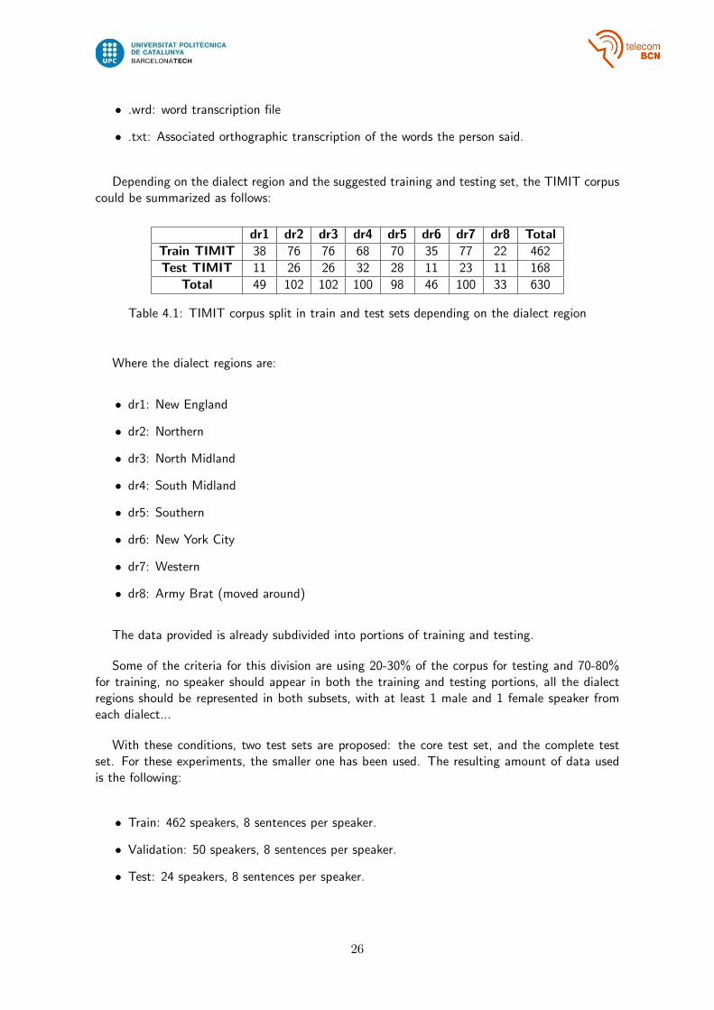
Depending on the dialect region and the suggested training and testing set, the TIMIT corpuscould be summarized as follows:

dr1 dr2 dr3 dr4 dr5 dr6 dr7 dr8 TotalTrain TIMIT 38 76 76 68 70 35 77 22 462

Test TIMIT 11 26 26 32 28 11 23 11 168

Total 49 102 102 100 98 46 100 33 630

Table 4.1: TIMIT corpus split in train and test sets depending on the dialect region

Where the dialect regions are:

• dr1: New England

• dr2: Northern

• dr3: North Midland

• dr4: South Midland

• dr5: Southern

• dr6: New York City

• dr7: Western

• dr8: Army Brat (moved around)

The data provided is already subdivided into portions of training and testing.

Some of the criteria for this division are using 20-30% of the corpus for testing and 70-80%for training, no speaker should appear in both the training and testing portions, all the dialectregions should be represented in both subsets, with at least 1 male and 1 female speaker fromeach dialect...

With these conditions, two test sets are proposed: the core test set, and the complete testset. For these experiments, the smaller one has been used. The resulting amount of data usedis the following:

• Train: 462 speakers, 8 sentences per speaker.

• Validation: 50 speakers, 8 sentences per speaker.

• Test: 24 speakers, 8 sentences per speaker.

26

4.3 Evaluation metric

The evaluation of Speech recognition models, as well as machine translation ones, is usuallydone with WER metric: Word Error Rate. The main difficulty when measuring performance isthat the recognized sequence can have a different length from the reference one. That is why itis not possible to evaluate the models only looking at the mistakes: it is also necessary to knowthe insertions or the deletions. It is defined like this:

WER =Sw +Dw + Iw

Nw(4.1)

Where,

• Sw: number of substitutions

• Dw: number of deletions

• Iw: number of insertions

• Nw: number of words in the reference sentence.

This metric is used working at the word level, but as TIMIT uses phonemes, the proper metricto be used is PER: Phoneme Error Rate. The way to compute it is quite similar, but using thetotal number N of phonemes and the minimal number of character insertions I, substitutions Sand deletions D required to transform the reference text into the output.

Since the number of mistakes can be larger than the length of the reference text and lead torates large than 100% (for example, a ground-truth sentence with 100 phonemes and an outputwhich contains 120 wrong phonemes give a 120% error rate), sometimes the number of mistakesis divided by the sum (I + S + D + C ): the number of edit operations (I + S + D) and thenumber C of correct symbols, which is always larger than the numerator.

Another way to evaluate this kind of datasets is computing the accuracy. In this case we justneed to substract 100-PER:

Accuracy = 100− PER =Nw − S −D − I

Nwx100% (4.2)

4.4 Experiment analysis

The model was only trained with the TIMIT corpus, but different setups have been tried.

Apart from the differences between the Nabu’s parameters and the paper ones (Section 3.2.1,two different trainers (Section 3.2.3) have been tried: the standard one and the fisher one. Thefisher trainer uses the Fisher Information Matrix, which essentially determines the asymptoticbehavior of the estimator[12][22]

27

In all the experiments, the frequency of evaluating the validation set is every 500 steps, andthe number of times the validation performance can be worse before terminating the training isfive. If after a worse validation comes a better one, the the number of tries (5) is reset.

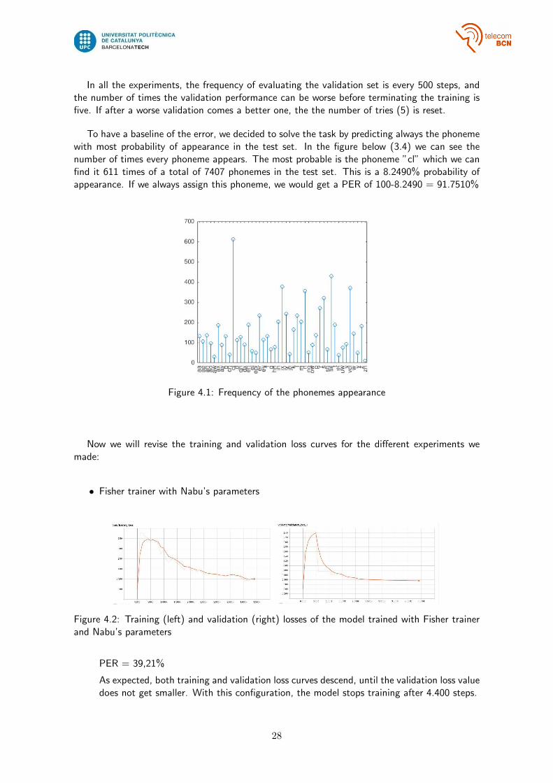
To have a baseline of the error, we decided to solve the task by predicting always the phonemewith most probability of appearance in the test set. In the figure below (3.4) we can see thenumber of times every phoneme appears. The most probable is the phoneme ”cl” which we canfind it 611 times of a total of 7407 phonemes in the test set. This is a 8.2490% probability ofappearance. If we always assign this phoneme, we would get a PER of 100-8.2490 = 91.7510%

Figure 4.1: Frequency of the phonemes appearance

Now we will revise the training and validation loss curves for the different experiments wemade:

• Fisher trainer with Nabu’s parameters

Figure 4.2: Training (left) and validation (right) losses of the model trained with Fisher trainerand Nabu’s parameters

PER = 39,21%

As expected, both training and validation loss curves descend, until the validation loss valuedoes not get smaller. With this configuration, the model stops training after 4.400 steps.

28

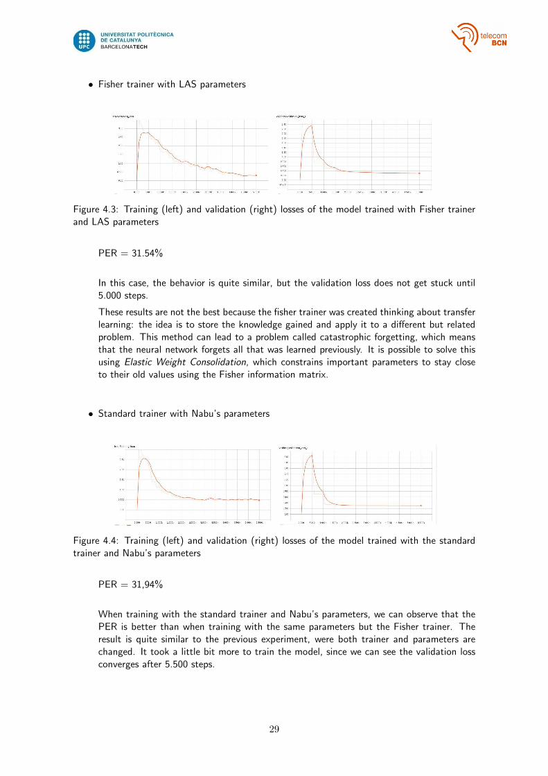
• Fisher trainer with LAS parameters

Figure 4.3: Training (left) and validation (right) losses of the model trained with Fisher trainerand LAS parameters

PER = 31.54%

In this case, the behavior is quite similar, but the validation loss does not get stuck until5.000 steps.

These results are not the best because the fisher trainer was created thinking about transferlearning: the idea is to store the knowledge gained and apply it to a different but relatedproblem. This method can lead to a problem called catastrophic forgetting, which meansthat the neural network forgets all that was learned previously. It is possible to solve thisusing Elastic Weight Consolidation, which constrains important parameters to stay closeto their old values using the Fisher information matrix.

• Standard trainer with Nabu’s parameters

Figure 4.4: Training (left) and validation (right) losses of the model trained with the standardtrainer and Nabu’s parameters

PER = 31,94%

When training with the standard trainer and Nabu’s parameters, we can observe that thePER is better than when training with the same parameters but the Fisher trainer. Theresult is quite similar to the previous experiment, were both trainer and parameters arechanged. It took a little bit more to train the model, since we can see the validation lossconverges after 5.500 steps.

29

• Standard trainer with LAS parameters

Figure 4.5: Training (left) and validation (right) losses of the model trained with standard trainerand LAS parameters

PER = 27.29%

This is our best result and it is obtained using the standard trainer and the parametersdefined in the paper.

The behavior of both models trained with the standard trainer is quite similar. We can seethat the main difference is that with LAS parameters the validation loss does not convergeuntil 7.500 steps, while with Nabu’s parameters it stops at 5.000 steps.

Model DEV TESTFisher trainer and Nabu’s parameters 36.36% 39.21%

Fisher trainer and LAS parameters 29.92% 31.54%Standard trainer and Nabu’s parameters 30.20% 31.94%

Standard trainer and LAS parameters 25.12% 27.29%

Table 4.2: Phoneme error rates of evaluated models

As in the TIMIT corpus it is defined the train and test sets (Section 4.2) we can comparethe results to other experiments that have been carried out with the Core Test Set (the one weused).

Model DEV TESTLarge margin GMM[28] -% 33%

CTC end to end training[17] 19.05% 21.97%DBLSTM hybrid training[17] 17.44% 19.34%

CNN limited weight sharing[2] - 20.50%Bayesian triphone HMM[24] - 25.6%

CNN 3hidden layer (no pre-training)[3] - 20.07%RNN seq2seq with attention end-to-end training(our work) 25.12% 27.29%

Table 4.3: Reported results on TIMIT Core Test Set

30

Chapter 5

Budget

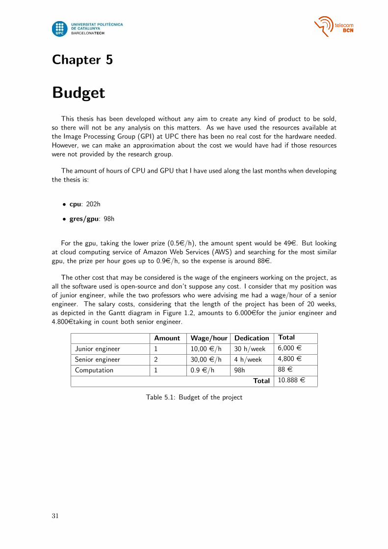
This thesis has been developed without any aim to create any kind of product to be sold,so there will not be any analysis on this matters. As we have used the resources available atthe Image Processing Group (GPI) at UPC there has been no real cost for the hardware needed.However, we can make an approximation about the cost we would have had if those resourceswere not provided by the research group.

The amount of hours of CPU and GPU that I have used along the last months when developingthe thesis is:

• cpu: 202h

• gres/gpu: 98h

For the gpu, taking the lower prize (0.5e/h), the amount spent would be 49e. But lookingat cloud computing service of Amazon Web Services (AWS) and searching for the most similargpu, the prize per hour goes up to 0.9e/h, so the expense is around 88e.

The other cost that may be considered is the wage of the engineers working on the project, asall the software used is open-source and don’t suppose any cost. I consider that my position wasof junior engineer, while the two professors who were advising me had a wage/hour of a seniorengineer. The salary costs, considering that the length of the project has been of 20 weeks,as depicted in the Gantt diagram in Figure 1.2, amounts to 6.000efor the junior engineer and4.800etaking in count both senior engineer.

Amount Wage/hour Dedication Total

Junior engineer 1 10,00 e/h 30 h/week 6,000 e

Senior engineer 2 30,00 e/h 4 h/week 4,800 e

Computation 1 0.9 e/h 98h 88 e

Total 10.888 e

Table 5.1: Budget of the project

31

Chapter 6

Conclusions

This project’s main goal has been to train an end-to-end speech recognition system so it canbe used in the Speech2Signs project or in any future work of the TALP research group at UPC. Asshown in the current manuscript, we have successfully accomplished this main goal. To achievesuch objective, we have reached a better understanding of the techniques used to process speechin the deep learning framework through the process of running the speech recognition system.

This has not been an easy journey and we are not saying that there is no space for improve-ments, but we had the chance to learn about one of the most trendy approaches in speechrecognition from the very last years.

After facing with an under-development implementation, it took more time than expectedto have the system working, so it let us few time to make the experiments (like trying otherdatasets). However, we finally have trained an end-to-end model with sequence to sequencelearning improved with the attention mechanism, and tried it with different configurations inorder to obtain the lowest Phoneme Error Rate.

The system we have been working on was proposed in Listen, Attend and Spell (LAS)[6].LAS is trained end-to-end and has two main components. The first component, the listener, isa pyramidal acoustic RNN encoder that transforms the input sequence into a high level featurerepresentation. The second component, the speller, is an RNN decoder that attends to this highlevel features and spells out one character at a time. The main difference in the implementedsystem is that we have trained it with a phoneme-based dataset (TIMIT) instead of using word-based datasets.

As a future work, we want to change the dataset to another one not containing phonemes butwords, and then the system will be ready to be used as the first module of Speech2Signs. Also,we want to reproduce fresh new research (from 18th January 2018) that furhter extends the LASarchitecture by using an improved attention mechanism (i.e. based on multi-heads) [7].

32

Bibliography

[1] Martın Abadi, Ashish Agarwal, Paul Barham, Eugene Brevdo, Zhifeng Chen, Craig Citro,Greg S. Corrado, Andy Davis, Jeffrey Dean, Matthieu Devin, Sanjay Ghemawat, Ian Good-fellow, Andrew Harp, Geoffrey Irving, Michael Isard, Yangqing Jia, Rafal Jozefowicz, LukaszKaiser, Manjunath Kudlur, Josh Levenberg, Dan Mane, Rajat Monga, Sherry Moore, DerekMurray, Chris Olah, Mike Schuster, Jonathon Shlens, Benoit Steiner, Ilya Sutskever, KunalTalwar, Paul Tucker, Vincent Vanhoucke, Vijay Vasudevan, Fernanda Viegas, Oriol Vinyals,Pete Warden, Martin Wattenberg, Martin Wicke, Yuan Yu, and Xiaoqiang Zheng. Ten-sorFlow: Large-scale machine learning on heterogeneous systems, 2015. Software availablefrom tensorflow.org.

[2] Ossama Abdel-Hamid, Li Deng, and Dong Yu. Exploring convolutional neural networkstructures and optimization techniques for speech recognition. In Interspeech, pages 3366–3370, 2013.

[3] Ossama Abdel-Hamid, Abdel-rahman Mohamed, Hui Jiang, and Gerald Penn. Applyingconvolutional neural networks concepts to hybrid nn-hmm model for speech recognition. InAcoustics, Speech and Signal Processing (ICASSP), 2012 IEEE International Conference on,pages 4277–4280. IEEE, 2012.

[4] Students at DePaul University. The american sign language avatar project. http://asl.

cs.depaul.edu.

[5] Dzmitry Bahdanau, Jan Chorowski, Dmitriy Serdyuk, Philemon Brakel, and Yoshua Bengio.End-to-end attention-based large vocabulary speech recognition. In Acoustics, Speech andSignal Processing (ICASSP), 2016 IEEE International Conference on, pages 4945–4949.IEEE, 2016.

[6] William Chan, Navdeep Jaitly, Quoc V Le, and Oriol Vinyals. Listen, attend and spell. arXivpreprint arXiv:1508.01211, 2015.

[7] Chung-Cheng Chiu, Tara N Sainath, Yonghui Wu, Rohit Prabhavalkar, Patrick Nguyen,Zhifeng Chen, Anjuli Kannan, Ron J Weiss, Kanishka Rao, Katya Gonina, et al. State-of-the-art speech recognition with sequence-to-sequence models. arXiv preprint arXiv:1712.01769,2017.

[8] Jan K Chorowski, Dzmitry Bahdanau, Dmitriy Serdyuk, Kyunghyun Cho, and Yoshua Ben-gio. Attention-based models for speech recognition. In Advances in Neural InformationProcessing Systems, pages 577–585, 2015.

[9] FA Chowdhury, Quan Wang, Ignacio Lopez Moreno, and Li Wan. Attention-based modelsfor text-dependent speaker verification. arXiv preprint arXiv:1710.10470, 2017.

[10] Jeffrey Dean, Greg S. Corrado, Rajat Monga, Kai Chen, Matthieu Devin, Quoc V. Le,Mark Z. Mao, Marc’Aurelio Ranzato, Andrew Senior, Paul Tucker, Ke Yang, and Andrew Y.Ng. Large scale distributed deep networks. In NIPS, 2012.

[11] Sean R Eddy. Hidden markov models. Current opinion in structural biology, 6(3):361–365,1996.

[12] Kenji Fukumizu. A regularity condition of the information matrix of a multilayer perceptronnetwork. Neural networks, 9(5):871–879, 1996.

33

[13] Mark Gales and Steve Young. The application of hidden markov models in speech recogni-tion. Foundations and trends in signal processing, 1(3):195–304, 2008.

[14] J-L Gauvain and Chin-Hui Lee. Maximum a posteriori estimation for multivariate gaussianmixture observations of markov chains. IEEE transactions on speech and audio processing,2(2):291–298, 1994.

[15] Alex Graves, Santiago Fernandez, Faustino Gomez, and Jurgen Schmidhuber. Connectionisttemporal classification: labelling unsegmented sequence data with recurrent neural networks.In Proceedings of the 23rd international conference on Machine learning, pages 369–376.ACM, 2006.

[16] Alex Graves and Navdeep Jaitly. Towards end-to-end speech recognition with recurrentneural networks. In Proceedings of the 31st International Conference on Machine Learning(ICML-14), pages 1764–1772, 2014.

[17] Alex Graves, Navdeep Jaitly, and Abdel-rahman Mohamed. Hybrid speech recognition withdeep bidirectional lstm. In Automatic Speech Recognition and Understanding (ASRU), 2013IEEE Workshop on, pages 273–278. IEEE, 2013.

[18] Alex Graves, Abdel-rahman Mohamed, and Geoffrey Hinton. Speech recognition with deeprecurrent neural networks. In Acoustics, speech and signal processing (icassp), 2013 ieeeinternational conference on, pages 6645–6649. IEEE, 2013.

[19] Geoffrey Hinton, Li Deng, Dong Yu, George E Dahl, Abdel-rahman Mohamed, NavdeepJaitly, Andrew Senior, Vincent Vanhoucke, Patrick Nguyen, Tara N Sainath, et al. Deepneural networks for acoustic modeling in speech recognition: The shared views of fourresearch groups. IEEE Signal Processing Magazine, 29(6):82–97, 2012.

[20] Sergey Ioffe and Christian Szegedy. Batch normalization: Accelerating deep network trainingby reducing internal covariate shift. In International Conference on Machine Learning, pages448–456, 2015.

[21] William M. Fisher Jonathan G. Fiscus David S. Pallett Nancy L. Dahlgren Victor Zue JohnS. Garofolo, Lori F. Lamel. Timit acoustic-phonetic continuous speech corpus. In LinguisticData Consortium, 1993.

[22] Alexander Ly, Maarten Marsman, Josine Verhagen, Raoul Grasman, and Eric-Jan Wagen-makers. A tutorial on fisher information. arXiv preprint arXiv:1705.01064, 2017.

[23] Daniel Moreno Manzano. English to american sign language translator in the context ofspeech2signs project. 2018.

[24] Ji Ming and F Jack Smith. Improved phone recognition using bayesian triphone models. InAcoustics, Speech and Signal Processing, 1998. Proceedings of the 1998 IEEE InternationalConference on, volume 1, pages 409–412. IEEE, 1998.

[25] Daniel Povey, Arnab Ghoshal, Gilles Boulianne, Lukas Burget, Ondrej Glembek, NagendraGoel, Mirko Hannemann, Petr Motlicek, Yanmin Qian, Petr Schwarz, Jan Silovsky, GeorgStemmer, and Karel Vesely. The kaldi speech recognition toolkit. In IEEE 2011 Workshopon Automatic Speech Recognition and Understanding. IEEE Signal Processing Society, De-cember 2011. IEEE Catalog No.: CFP11SRW-USB.

[26] Vincent Renkens. Nabu. https://github.com/vrenkens/nabu, 2017.

34

[27] Hasim Sak, Andrew Senior, and Francoise Beaufays. Long short-term memory recurrent neu-ral network architectures for large scale acoustic modeling. In Fifteenth Annual Conferenceof the International Speech Communication Association, 2014.

[28] Fei Sha and Lawrence K Saul. Large margin gaussian mixture modeling for phonetic classi-fication and recognition. In Acoustics, Speech and Signal Processing, 2006. ICASSP 2006Proceedings. 2006 IEEE International Conference on, volume 1, pages I–I. IEEE, 2006.

[29] Nitish Srivastava, Geoffrey E Hinton, Alex Krizhevsky, Ilya Sutskever, and Ruslan Salakhut-dinov. Dropout: a simple way to prevent neural networks from overfitting. Journal ofmachine learning research, 15(1):1929–1958, 2014.

[30] R Wilbur. American sign language. 1987.

35