CZECH TECHNICAL UNIVERSITY IN PRAGUE

Faculty of Electrical Engineering

DIPLOMA THESIS

Viktor Kozak

Exploration of an Unknown Space with a Mobile Robot

Department of Cybernetics

Thesis supervisor: RNDr. Miroslav Kulich, Ph.D.

May, 2017

Czech Technical University in Prague Faculty of Electrical Engineering

Department of Cybernetics

DIPLOMA THESIS ASSIGNMENT

Student: Bc. Viktor K o z á k

Study programme: Cybernetics and Robotics

Specialisation: Robotics

Title of Diploma Thesis: Exploration of an Unknown Space with a Mobile Robot

Guidelines: 1. Get acquainted with current state of the framework EAPD (Exploration Algorithm in a Polygonal Domain) for mobile robot exploration[1] and with ROS (Robot Operating System) [2]. 2. Get acquainted with methods of simultaneous localization and mapping. 3. Choose an appropriate open source implementation of SLAM for laser rangefinder and experimentally verify its behavior with real data. Focus on computational complexity, precision of computed position in various environments. 4. Integrate the chosen SLAM library into EAPD. 5. Design and implement refinement of a polygonal map generated by EAPD in case loop closing is detected by the SLAM algorithm. 6. Verify experimentally the proposed solution with a real robot and describe and discuss obtained results. Bibliography/Sources: [1] http://imr.ciirc.cvut.cz/Research/EAPD [2] http://http://www.ros.org [3] Tomáš Juchelka: Exploration algorithms in a polygonal domain, Diploma Thesis, CTU in Prague, FEE, Dept. of Cybernetics, 2013 [4] Vojtěch Lhotský: An integrated approach to multi-robot exploration of an unknown space, Diploma Thesis, CTU in Prague, FEE, Dept. of Cybernetics, 2016 [5] Miroslav Kulich, Tomáš Juchelka, Libor Přeučil: Comparison of exploration strategies for multi-robot search, Acta Polytechnica , Vol. 55, No. 3 (2015), pp. 162-168

Diploma Thesis Supervisor: RNDr. Miroslav Kulich, Ph.D.

Valid until: the end of the summer semester of academic year 2017/2018

L.S.

prof. Dr. Ing. Jan Kybic Head of Department

prof. Ing. Pavel Ripka, CSc. Dean

Prague, February 17, 2017

Declaration

I declare that the presented work was developed independently and that I have listed allsources of information used within it in accordance with the methodical instructions for observingthe ethical principles in the preparation of university theses.

In Prague on............................. ...............................................

Acknowledgements

I would like to thank my thesis supervisor RNDr. Miroslav Kulich, Ph.D for his professionalleadership, advice on my work and for his patience with me. I would also like to thank all thepeople who supported me during my years at the university.

Abstrakt

Tato diplomova prace se zabyva prohledavanım neznameho prostredı mo-bilnım robotem. Robot je vybaven laserovym snımacem a behem exploraceje tvorena 2D polygonalnı mapa, tato cast prace navazuje na Exploracnı al-goritmy v polygonalnı domene od T. Juchelky[1]. V ramci prace byla do ex-ploracnıho algoritmu implementovana metoda pro uzavıranı smycek v mapea metoda pro zpetnou upravu a rekonstrukci mapy. Implementovane metodybyly otestovany s realnym robotem Turtle Bot v ruznych prostredıch.

Abstract

The subject of this diploma thesis is the exploration of an unknown spacewith a mobile robot. The robot is equipped with a laser rangefinder andcreates a 2D polygonal map, this part of the work follows and extends theExploration Algorithms in a Polygonal Domain thesis by T. Juchelka[1]. Newfunctionalities were implemented and added to the exploration algorithm, amethod for loop closing in the polygonal map and a method for the refine-ment of the polygonal map. The implemented methods were tested with areal TurtleBot robot in various environments.

CONTENTS

Contents

1 Introduction 1

2 Robot exploration 3

2.1 Simultaneous localization and mapping . . . . . . . . . . . . . . . . . . . . . 4

2.1.1 Gmapping . . . . . . . . . . . . . . . . . . . . . . . . . . . . . . . . 4

2.2 Mobile robot exploration . . . . . . . . . . . . . . . . . . . . . . . . . . . . . 5

2.2.1 Frontier selection and path planning . . . . . . . . . . . . . . . . . . . 6

2.2.2 Exploration using a 2D occupancy grid . . . . . . . . . . . . . . . . . 8

2.2.3 Topological graphs . . . . . . . . . . . . . . . . . . . . . . . . . . . . 8

2.2.4 Exploration in a polygonal domain . . . . . . . . . . . . . . . . . . . . 10

3 Introduction to EAPD 11

3.1 ROS - Robotic framework . . . . . . . . . . . . . . . . . . . . . . . . . . . . 11

3.2 EAPD . . . . . . . . . . . . . . . . . . . . . . . . . . . . . . . . . . . . . . 12

3.3 Integration of Gmapping with EAPD . . . . . . . . . . . . . . . . . . . . . . 15

4 Implementation of a loop closing algorithm 17

4.1 Introduction to the loop closing problem . . . . . . . . . . . . . . . . . . . . 17

4.1.1 Loop closure detection . . . . . . . . . . . . . . . . . . . . . . . . . . 17

4.1.2 Position and map correction . . . . . . . . . . . . . . . . . . . . . . . 20

4.1.3 Loop closure in Gmapping . . . . . . . . . . . . . . . . . . . . . . . . 20

4.2 Integration of the extended Gmapping functionality into EAPD . . . . . . . . 20

4.3 Implementation of polygonal map refinement in case of loop closure detection 22

i

CONTENTS

5 Experimental results 25

5.1 Hardware . . . . . . . . . . . . . . . . . . . . . . . . . . . . . . . . . . . . . 25

5.1.1 TurtleBot . . . . . . . . . . . . . . . . . . . . . . . . . . . . . . . . . 25

5.1.2 LaserRangefinder . . . . . . . . . . . . . . . . . . . . . . . . . . . . . 27

5.1.3 Intel NUC mini computer . . . . . . . . . . . . . . . . . . . . . . . . 28

5.2 Environment . . . . . . . . . . . . . . . . . . . . . . . . . . . . . . . . . . . 28

5.3 Results . . . . . . . . . . . . . . . . . . . . . . . . . . . . . . . . . . . . . . 30

5.3.1 The EAPD framework supported by the Gmapping SLAM algorithm . . 30

5.3.2 The EAPD framework with the use of the extended Gmapping functionality 32

5.3.3 Map refinement with a separate loop node . . . . . . . . . . . . . . . 34

5.4 Discussion of the results . . . . . . . . . . . . . . . . . . . . . . . . . . . . . 36

6 Conclusion 38

List of Figures 43

List of Tables 44

ii

Chapter 1

Introduction

Autonomous robot exploration is a widely used approach in mapping, search and rescueoperations. It is utilized to survey areas which might be dangerous or inaccessible by humans.Robots equipped with a wide range of sensors are used to build maps of the environment or tosearch for specific objects.

In this work an autonomous robot equipped with a laser rangefinder is used for explorationand map building. The focus of this work is on exploration in 2D polygonal domain, which offerscertain advantages in contrast to the more popular 2D occupancy grids. Maps in polygonaldomain are much more memory efficient, offering a big advantage in larger environments.On the other hand, algorithms designed for occupancy grids may be useless when handling apolygonal representation, thus arises the need to adjust these algorithms or implement moresuitable approaches.

The work follows and extends a framework implemented by T. Juchelka in his thesis Ex-ploration algorithms in a polygonal domain [1]. T. Juchelka implemented a general frameworkbased on polygonal representation of an environment in Robot Operating System (ROS)[2]. Itwas later extended and tested on real robots by V. Lhotsky in [3]. In Lhotsky’s work, robotsare equipped with an RGBD camera sensors allowing them to operate using the RTAB-Mappackage from ROS as its main SLAM algorithm.

In the first part of this work the EAPD algorithm is adjusted for the use with a real robotequipped with a laser rangefinder instead of the RGBD camera. Gmapping package from ROSwas selected as a suitable implementation of SLAM for a laser rangefinder, integrated into theEAPD package and tested on a real robot.

The second part of the work is focused on a refinement of the polygonal map, generatedby EAPD in case a loop closure is detected by the SLAM algorithm. Since there are morepossible methods for the detection of loop closures, these methods are discussed and the moreappropriate ones were selected for this work. Gmapping’s approach to the loop closure problemis closely connected with it’s internal structure, therefore EAPD and Gmapping packages wereadjusted to work together and appropriately react to loop closing related changes. Other possible

1/45

method more suitable for other SLAM packages is proposed and implemented separately, servingas a foundation for possible future uses with other approaches.

Chapter 2 gives the reader a short introduction to the theory of robotic exploration and coversbasic description of main approaches and main differences between them. This chapter alsocovers the theory of simultaneous localization and mapping and describes several approachesto the problem.

Chapter 3 describes the EAPD framework and its implementation in ROS. The basic inte-gration of Gmapping with EAPD is also covered here.

Chapter 4 describes the implementation of the loop closure detection in the EAPD framework.The chapter covers introduction to the loop closure problem first and than is divided in twoparts. The first part is dedicated to the integration of extended Gmapping functionality, such asloop closure, into the EAPD package. The second part covers the loop closure independentlyfrom the SLAM algorithm and is focused on the refinement of a polygonal map generated byEAPD.

Chapter 5 covers the description of the used hardware and the experiments on a TurtleBotmobile robot. The chapter presents:

1. Results of the use of Gmapping as a SLAM algorithm with the EAPD package.

2. Results gathered after modifying Gmapping and using extended Gmapping functionalityin EAPD. This part also covers loop closure by Gmapping.

3. The results for a general refinement of the polygonal map executed during the explorationprocess.

2/45

Chapter 2

Robot exploration

In the mobile robot exploration task a robot equipped with sensors is used to operate in anunknown environment in order to maximize the knowledge over a particular area. The robotautonomously navigates through it’s surroundings and builds a map of the environment. Theincrementally built map is then used as a base for selecting further goals of exploration. Therobot operates until it creates a complete map of the environment, or until it reaches somespecific goal, i.e. finds a specific target.

Although mobile robot exploration is most suited for surveying areas which might be inac-cessible or dangerous to humans, with a decrease in prices of small computer units and sensorequipment, mobile robot exploration became widely spread in other areas, increasing the needfor further improvement and optimization of current methods.

The problem of robot exploration can be split in two main parts. In the first part, the robothas to challenge the problem of creating a map of the environment and maintaining knowledgeabout its own position in accordance to the map. The second problem is the exploration itself,mainly the selection of next goals of the exploration and navigation through the environment.

The EAPD framework focuses on map building and exploration goal selection but requires asuitable position estimation. Our intent is to use the EAPD framework with a TurtleBot mobilerobot which provides basic movement odometry and is equipped with a laser rangefinder. Anappropriate method has to be selected to provide a suitable position estimate.

Even though there are algorithms that can provide position estimation based only on theodometry data and laser scans without creating a map of the environment, due to the noise anderror in these measurements, the estimated positions are often inaccurate and the accumulatederror after few iterations is unacceptable. Therefore we decided to select one of the algorithmsfor simultaneous localization and mapping (SLAM), which are more reliable. A comparison ofposition estimates based solely on the odometry data and estimates based on odometry andlaser scan is depicted in Fig. 2.1.

3/45

2.1. SIMULTANEOUS LOCALIZATION AND MAPPING

Figure 2.1: The left picture presents a visualization of particle distribution after a few iterationsbased on odometry. The right picture describes particle distribution based on odometry andlaser measurements in several specific environments. Pictures were taken from [6] and [5].

2.1 Simultaneous localization and mapping

The problem of simultaneous localization and mapping is often compared to the ”chickenand egg” problem. We need accurate position estimates to create a map using our observations,but we also need a good map of the environment to properly estimate the current position ofthe robot.

Since this work will be using the ROS framework, the focus on SLAM algorithms will beon those, that can be used with ROS and with a laser rangefinder. There are two suitablealgorithms already implemented in ROS, the Gmapping package and the Hector Slam package.Due to better overall response of users to the package and previous personal experience withit, the Gmapping package has been selected for the use with the EAPD framework.

A noticeable selection of SLAM algorithms can be found on the OpenSlam website[4], whichserves as a support for SLAM researchers and offers the possibility to publish their work. Someof these algorithms can also be used with ROS and provide extended functionalities. Thesealgorithms were often used as a reference, while working on the loop closure problem in thiswork.

2.1.1 Gmapping

Gmapping package, presented on the OpenSlam website and described in [5] and [7], was laterwrapped for the use with ROS and is maintained as a standard ROS package till date. Gmappingpresents a Rao-Blackwellized particle filter as an effective mean to solve the simultaneouslocalization and mapping problem.

This approach is based on a particle filter where each particle carries an individual map ofthe environment. A particle creates a grid map containing occupancy probabilities for each gridcell, representing a possible obstacle at its location. As such the computation and memoryrequirements are strongly dependent on the number of particles used in the algorithm. Due

4/45

2.2. MOBILE ROBOT EXPLORATION

to advanced filtering and resampling techniques used in Gmapping, the number of particlesrequired is relatively low and the default setting with 30 particles is usually sufficient for mostenvironments.

Gmapping computes an accurate distribution of particles taking into account the move-ment of the robot and the most recent observation. The key idea is to estimate a posteriorp(x1:t|z1:t, u0:t) about probable trajectories x1:t of the robot given its observations z1:t and itsodometry measurements u0:t. This posterior is further used to compute a posterior over mapsand trajectories:

p(x1:t,m|z1:t, u0:t) = p(m|x1:t, z1:t)p(x1:t|z1:t, u0:t) (2.1)

The process of the SLAM algorithm iteratively creates a map of the environment and updatespositions of the particles. Every iteration contents of 5 main steps[5]:

1. Sampling : New generation of particles x(i)t is obtained from the current generation x

(i)t−1

by sampling from a proposal distribution π(xt|z1:t, u0:t).

2. Importance weighting : Each particle is assigned an individual importance weight w(i)

according to:

w(i) =p(x

(i)t |z1:t)

π(x(i)t |z1:t)

(2.2)

These weights account for the fact that the proposal distribution π is in general not equalto the target distribution of successor states.

3. Resampling : Particles with low weights are replaced by samples with higher weights. Dueto a limited number of particles it is important to approximate a continuous distribution.Resampling also allows to apply a particle filter in situations in which the true distributiondiffers from the proposal.

4. Map Estimation: For each particle position x(i)t is computed a corresponding map esti-

mate m(i)t , based on the previous trajectory and the history of observations according to

p(m(i)1:t|x

(i)1:t, z1:t).

5. Output selection: The particle with the highest importance weight is determined as thebest particle and it’s position is published as the current position of the robot, togetherwith its corresponding map estimate.

2.2 Mobile robot exploration

With the problem of localization and mapping solved by the Gmapping package we cannow focus on the exploration itself. In the exploration problem the robot navigates through the

5/45

2.2. MOBILE ROBOT EXPLORATION

environment and incrementally updates a map which is used as a model for further explorationsteps. The other tasks of exploration algorithms are selection of future goals, planning andnavigation through the environment. A diagram describing the exploration process can be seenin Fig. 2.2. Individual parts of the diagram will be described in the next part of this chapter.

Figure 2.2: A diagram describing the exploration process.

While having some common basis, all of these operations are vastly dependent on the repre-sentation of the environment. This chapter will first describe the common base for all represen-tations. Features specific for other representations will be described later with a focus on themost popular 2D occupancy grid and the polygonal domain which will be used in this thesis.

2.2.1 Frontier selection and path planning

After completing the initial part of the map from robot’s starting position, the first task forexploration algorithms is to select the next desired position towards which the robot can moveto. Such task is usually connected with frontier selection.

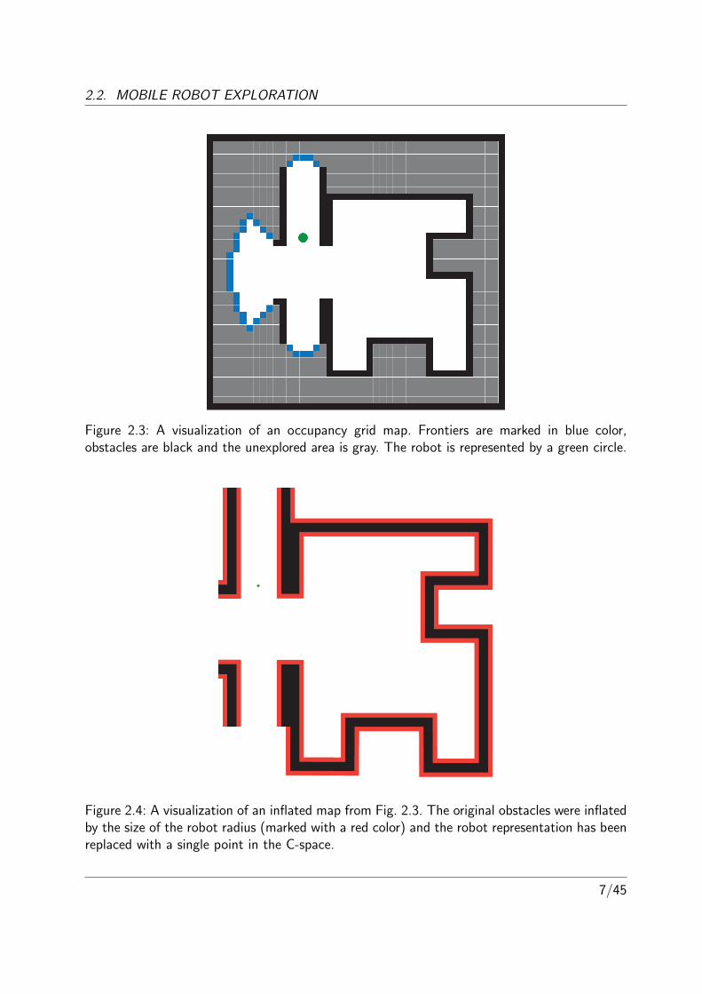
Frontiers can be described as borders between unoccupied and unexplored areas, these arethe parts which the robot has yet to explore. A visualization of frontiers over an occupancygrid is shown in Fig. 2.3. However not all frontiers are suitable for goal candidates, frontiersinaccessible by the robot or insignificantly small ones are generally excluded from the selection.Therefore when selecting a suitable frontier for a future exploration goal the frontiers have tobe filtered and the goal has to be selected from the remaining ones. In a situation where thereare no more exploration candidates, the robot usually reports the end of the exploration andeither terminates the exploration process or stays on stand by.

There are many possible approaches to frontier selection, one of the easiest is the selectionof the frontier closest to the robot. Other techniques are more closely connected with path

6/45

2.2. MOBILE ROBOT EXPLORATION

Figure 2.3: A visualization of an occupancy grid map. Frontiers are marked in blue color,obstacles are black and the unexplored area is gray. The robot is represented by a green circle.

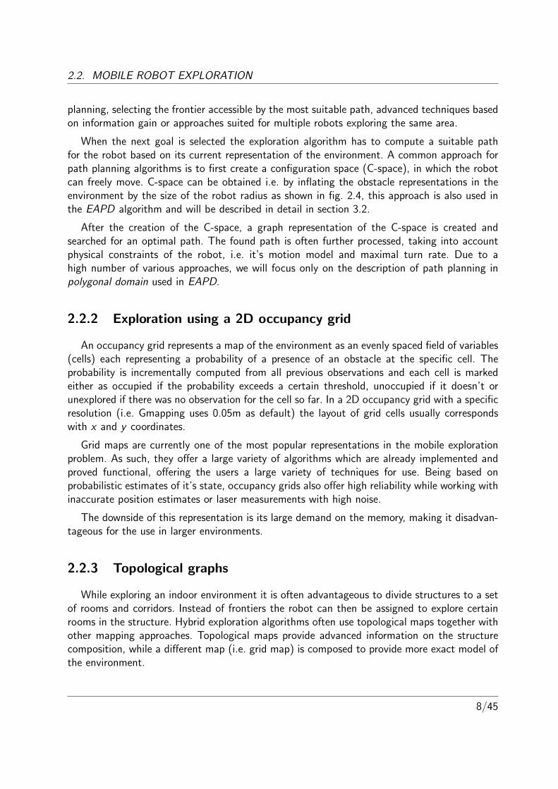
Figure 2.4: A visualization of an inflated map from Fig. 2.3. The original obstacles were inflatedby the size of the robot radius (marked with a red color) and the robot representation has beenreplaced with a single point in the C-space.

7/45

2.2. MOBILE ROBOT EXPLORATION

planning, selecting the frontier accessible by the most suitable path, advanced techniques basedon information gain or approaches suited for multiple robots exploring the same area.

When the next goal is selected the exploration algorithm has to compute a suitable pathfor the robot based on its current representation of the environment. A common approach forpath planning algorithms is to first create a configuration space (C-space), in which the robotcan freely move. C-space can be obtained i.e. by inflating the obstacle representations in theenvironment by the size of the robot radius as shown in fig. 2.4, this approach is also used inthe EAPD algorithm and will be described in detail in section 3.2.

After the creation of the C-space, a graph representation of the C-space is created andsearched for an optimal path. The found path is often further processed, taking into accountphysical constraints of the robot, i.e. it’s motion model and maximal turn rate. Due to ahigh number of various approaches, we will focus only on the description of path planning inpolygonal domain used in EAPD.

2.2.2 Exploration using a 2D occupancy grid

An occupancy grid represents a map of the environment as an evenly spaced field of variables(cells) each representing a probability of a presence of an obstacle at the specific cell. Theprobability is incrementally computed from all previous observations and each cell is markedeither as occupied if the probability exceeds a certain threshold, unoccupied if it doesn’t orunexplored if there was no observation for the cell so far. In a 2D occupancy grid with a specificresolution (i.e. Gmapping uses 0.05m as default) the layout of grid cells usually correspondswith x and y coordinates.

Grid maps are currently one of the most popular representations in the mobile explorationproblem. As such, they offer a large variety of algorithms which are already implemented andproved functional, offering the users a large variety of techniques for use. Being based onprobabilistic estimates of it’s state, occupancy grids also offer high reliability while working withinaccurate position estimates or laser measurements with high noise.

The downside of this representation is its large demand on the memory, making it disadvan-tageous for the use in larger environments.

2.2.3 Topological graphs

While exploring an indoor environment it is often advantageous to divide structures to a setof rooms and corridors. Instead of frontiers the robot can then be assigned to explore certainrooms in the structure. Hybrid exploration algorithms often use topological maps together withother mapping approaches. Topological maps provide advanced information on the structurecomposition, while a different map (i.e. grid map) is composed to provide more exact model ofthe environment.

8/45

2.2. MOBILE ROBOT EXPLORATION

A topological map is a set of places represented as graph nodes and linked by edges. Eachnode and edge can have additional characteristics used as a base for exploration algorithmsor data processing. For example, gate or doorway nodes are often used as nodes in betweenseparate rooms, providing the width of the gate and helping further exploration decisions.

A hybrid approach connecting the topological representation with an occupancy grid mapwas presented in [8]. The method divides the metrical grid map in equally sized segmentsand uses these segments as a base for the topological representation. Each segment is thenrepresented by an area node and the connections between neighboring cells are represented bygateway nodes. An example of the environment representation can be seen in Fig. 2.5.

Figure 2.5: A visualization of a topological map overlay over a metric map. The area nodes arerepresented by blue circles and the gateway nodes are represented by yellow rectangles.

The advantage of this approach is the connection of global planning over the topological mapand local planning in the individual segments of the grid map. The global plan is calculatedusing the topological representation and the local planning is computed whenever the robotenters a new segment in the metric map. Using this approach, there is no need to computethe full plan over the grid map at once reducing the peaks in the computation complexity. Thisapproach also reduces the complexity when the desired path is changed midway, as there is noneed to compute the path over the remaining grid map segments.

9/45

2.2. MOBILE ROBOT EXPLORATION

2.2.4 Exploration in a polygonal domain

T. Juchelka introduced polygonal domain representation and provided an usable frame-work for exploration in [1]. A map representation in a polygonal domain has significantly lowermemory requirements than the occupancy grid while preserving a higher detail. The polygonalrepresentation also allows easier processing in various ways, i.e. rotation or scaling.

This representation is based on polygons, defined by a finite number of line segments. Thesesegments are called edges, and a point where two edges meet is called a vertex. Vertexes arerepresented by their x, y coordinates and the type of edges leading in and out. A map iscomposed of edges representing either obstacles or frontiers as can bee seen in Fig. 2.6. Themap is focused only on relevant parts of the environment, thus demanding less memory. Withinthe map the inside of the polygon containing the robot is the unoccupied space.

Figure 2.6: A polygonal representation of the map from Fig. 2.3. The obstacles are marked inred color and the frontiers are marked blue.

The occupancy grid approach is advantageous over the polygonal in two main aspects.The first advantage of the occupancy grid is easier calculation of posterior probability of pastmeasurements in relation to the map. Secondly, as it has been more popular, a large varietyof support tools has already been implemented for the occupancy grid and these tools are stillmissing for the polygonal domain. This work addresses the second issue, proposing a tool forthe processing of a loop closure occurrence.

10/45

Chapter 3

Introduction to EAPD

The Exploration Algorithms in a Polygonal Domain(EAPD) framework was created by T.Juchelka[1], and was later extended by V. Lhotsky[3]. The framework was implemented inC++ as a ROS package and allows exploration in a polygonal domain using various explorationstrategies. This chapter contains a brief introduction to ROS followed by a description of theEAPD framework and later the integration of Gmapping SLAM algorithm.

3.1 ROS - Robotic framework

The Robot Operating System(ROS) is an open-source set of libraries and tools for develop-ment of robot applications. More information on ROS can be found on its official website [2].ROS offers a large set of drivers, state-of-art algorithms and developer tools.

ROS employs a system based on nodes, separate executables which can be individuallydesigned and run. Nodes perform individual tasks and ROS provides communication betweenthem in the form of standardized messages published on specific topics. These topics work asbroadcasts and any other node is able to receive the message. The separation of the processin individual nodes allows each subprocess (/node) to be written in different language, runon different frequency and to be modified without affecting the rest of the system. It is alsobeneficial as two nodes with similar functionalities can be easily exchanged.

Most important ROS tools used for work in this thesis are:

Rviz - a framework used for the visualization of broadcasted topic messages such as robotposition, map and laser scans.

RQT - a framework fro GUI development for ROS.

Catkin - a low-level build system macros and infrastructure for ROS.

TF package - a highly practical tool for handling transformations between coordinate framesover time. This is useful while handling positioning of sensors on the robot and robot positions

11/45

3.2. EAPD

in relation to the map. An example of robotic transformations in the system can be seen in Fig.3.1 created with the help of the RQT development tool.

Figure 3.1: A visualization of transformation frames in ROS. The image presents connectionsbetween individual coordinate frames.

ROS also provides a launch file system allowing an user to run more nodes at the sametime. Launch files also provide other useful options, such as setting parameters for the nodesat the startup, remapping specific topics or directly changing specific ROS settings. All lunchfiles used in this work are available on the CD, provided with the thesis.

3.2 EAPD

The EAPD package implemented in C++ allows exploration in a polygonal domain, provid-ing three main applications executable as individual ROS nodes and supported by other ROSlibraries. Those nodes are:

Robot node

The robot node receives data from laser scans and listens to transformations between coor-dinate systems. The information is processed and published after a transformation to a globalmap. While using several robots, each of them runs its own robot node which is dedicated toits own specific topics.

The robot node also listens to the path planning topic from the planner node and setsnavigation goals to the Smooth Nearness Diagram (SND) algorithm [9], integrated into the

12/45

3.2. EAPD

EAPD package. The SND algorithm is responsible for local navigation and obstacle avoidance,commanding the robot velocities with the help of laser-scan and odometry data.

The node subscribes to topics:

• /robot_i/base_scan - scan messages from the laser rangefinder, with relation to thei -th robot

• /robot_i/path - path messages from the planner node

The node publishes messages on topics:

• /laser_scan - laser scans published to the global map. This topic concentrates lasermessages from all robots.

• /robot_i/cmd_vel - velocity command

Map node

The map node subscribes to laser-scan data and listens to transformations from the robots.This node creates a polygonal map of the environment with a help from the clipping library[10].The map is then published for the planning node and optionally visualized in Rviz.

The node maintains a map in a form of two polygonal structures separated to represent thefree-space and obstacles independently. Every measurement is split into obstacles and frontiersand merged with the map. The map representation is later extended by offsetting the mapaccounting for the size of the robot during the planning process. The offset representation iskept separately. An example of the offset map can be seen in Fig. 3.2.

The node subscribes to topics:

• /laser_scan - laser scan messages from the robot node

The node publishes messages on topics:

• /map_global - global map for all robots

• /visualization_marker - visualization related to the map

13/45

3.2. EAPD

Figure 3.2: An example an offset polygonal map.

Figure 3.3: An example of a visibility graph.

14/45

3.3. INTEGRATION OF GMAPPING WITH EAPD

Planner node

The planner node is responsible for frontier selection and path planning. The node receivesthe map and selects a frontier as an exploration goal based on the exploration strategy. Thena suitable path is computed and published for the robot node.

The path planing itself uses Dijkstra algorithm with the use of a visibility graph, created fromthe polygonal map. The visibility graph is created from vertices in the map polygons. Thesevertices are taken as nodes in the graph and the nodes are adjacent (connected with an edge)if they can see each other. An example of a visibility graph is shown in Fig. 3.3.

The node subscribes to topics:

• /map_global - global map for all robots

The node publishes messages on topics:

• /robot_i/path - path goals published to a specific robot

• /planning - visualization related to the planning

3.3 Integration of Gmapping with EAPD

As a part of this thesis the Gmapping SLAM algorithm described in 2.1.1 was integrated intothe EAPD package to provide an accurate position estimate. ROS is based on a system usingindependent nodes, therefore adding the Gmapping node is relatively easy. After launching thenode, it tries to subscribe to the tf topic providing coordinate system transformations for thelaser, base and odometry, and to the scan topic for the laser measurements. An entry addingthe Gmapping node to the launch file can be seen in Listing 3.1.

<node pkg="gmapping" type="slam_gmapping" name="slam_gmapping" args="scan

:=robot_0/base_scan _base_frame:=robot_0/base_link" >

<param name="linearUpdate" value="0.3" />

<param name="angularUpdate" value="0.05" />

<param name="maxUrange" value="5" />

</node>

Listing 3.1: Gmapping SLAM section in the launch file.

The entry starts the slam_gmapping node from the Gmapping package, under the samename. The parameters set are the linearUpdate and angularUpdate Gmapping parameters,defining the change in robot position after which the grid map in Gmapping should be updated,while the maxUrange parameter limits the maximal range of a laser scan, that should be takeninto account, these parameters affect the inner process of Gmapping.

15/45

3.3. INTEGRATION OF GMAPPING WITH EAPD

A special focus should be on the args section. In this section topics scan and _base_frame

are remapped to topics robot_0/base_scan and robot_0/base_link respectively. Since thetransformation and laser scan topics are bound to a specific robot and can be used undervarious names, the gmapping node has to be informed which topics it should listen to. TheEAPD framework was developed to work with multiple robots, therefore its topics are numberedand dedicated to individual robots.

16/45

Chapter 4

Implementation of a loop closingalgorithm

As a part of this work, the refinement of a polygonal map in case of a loop closure detectionwas implemented. Introduction to the loop closure problem as well as to current approachesin the area are given in the first part of the chapter, followed by the integration of Gmappingloop closure detection into the EPAD package. Gmapping has a specific approach to the topic,therefore another method on refining of the map was proposed and implemented. This methodis described in the end of the chapter.

4.1 Introduction to the loop closing problem

A loop closure refers to a situation where a robot circles some part of the environment anddetects that it has already been at the same place before. A visualization of such situation canbe seen in figure 4.1, where we can see the real path of the robot, the estimated path and therequired loop closure correction. At that point the loop closing algorithm tries to correct robot’sposition, trajectory and map accordingly. Such correction can vastly improve the robustness oflocalization and mapping algorithms.

Current approaches regarding the problem differ both in the way the robot detects the loopclosure and the way the robot deals with the position and map correction. These differences arevastly dependent on equipped sensors, map representation and algorithms used for localizationand mapping.

4.1.1 Loop closure detection

The robot deals with several difficulties when determining if his current position correspondswith some of the previous positions.

17/45

4.1. INTRODUCTION TO THE LOOP CLOSING PROBLEM

Figure 4.1: A visualization of a loop closure.

Figure 4.2: A close-up of figure 4.1. The loop closure correction is marked with a blue arrow.The correction values x, y and yaw are depicted in the visualization.

18/45

4.1. INTRODUCTION TO THE LOOP CLOSING PROBLEM

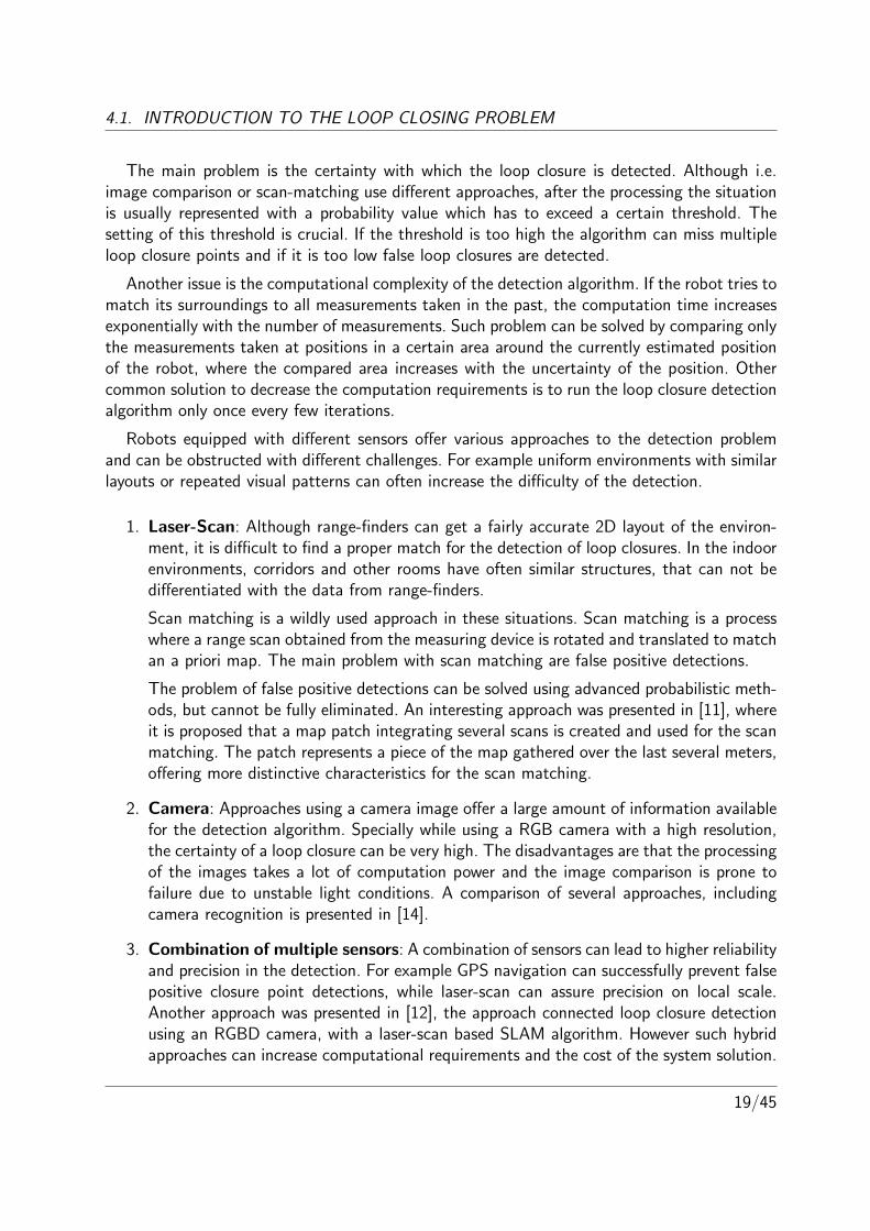
The main problem is the certainty with which the loop closure is detected. Although i.e.image comparison or scan-matching use different approaches, after the processing the situationis usually represented with a probability value which has to exceed a certain threshold. Thesetting of this threshold is crucial. If the threshold is too high the algorithm can miss multipleloop closure points and if it is too low false loop closures are detected.

Another issue is the computational complexity of the detection algorithm. If the robot tries tomatch its surroundings to all measurements taken in the past, the computation time increasesexponentially with the number of measurements. Such problem can be solved by comparing onlythe measurements taken at positions in a certain area around the currently estimated positionof the robot, where the compared area increases with the uncertainty of the position. Othercommon solution to decrease the computation requirements is to run the loop closure detectionalgorithm only once every few iterations.

Robots equipped with different sensors offer various approaches to the detection problemand can be obstructed with different challenges. For example uniform environments with similarlayouts or repeated visual patterns can often increase the difficulty of the detection.

1. Laser-Scan: Although range-finders can get a fairly accurate 2D layout of the environ-ment, it is difficult to find a proper match for the detection of loop closures. In the indoorenvironments, corridors and other rooms have often similar structures, that can not bedifferentiated with the data from range-finders.

Scan matching is a wildly used approach in these situations. Scan matching is a processwhere a range scan obtained from the measuring device is rotated and translated to matchan a priori map. The main problem with scan matching are false positive detections.

The problem of false positive detections can be solved using advanced probabilistic meth-ods, but cannot be fully eliminated. An interesting approach was presented in [11], whereit is proposed that a map patch integrating several scans is created and used for the scanmatching. The patch represents a piece of the map gathered over the last several meters,offering more distinctive characteristics for the scan matching.

2. Camera: Approaches using a camera image offer a large amount of information availablefor the detection algorithm. Specially while using a RGB camera with a high resolution,the certainty of a loop closure can be very high. The disadvantages are that the processingof the images takes a lot of computation power and the image comparison is prone tofailure due to unstable light conditions. A comparison of several approaches, includingcamera recognition is presented in [14].

3. Combination of multiple sensors: A combination of sensors can lead to higher reliabilityand precision in the detection. For example GPS navigation can successfully prevent falsepositive closure point detections, while laser-scan can assure precision on local scale.Another approach was presented in [12], the approach connected loop closure detectionusing an RGBD camera, with a laser-scan based SLAM algorithm. However such hybridapproaches can increase computational requirements and the cost of the system solution.

19/45

4.2. INTEGRATION OF THE EXTENDED GMAPPING FUNCTIONALITY INTO EAPD

4.1.2 Position and map correction

Once the loop closure is successfully detected, the algorithm has to integrate this newknowledge into its beliefs. Simple update of the current position could be made but dependingon the application, different parts of the program can be affected.

The algorithm might try to update information on previous paths and refine the generatedmap, based on the loop closure correction. This requires information on the previous states ofthe robot and knowledge of the starting point of the loop. The implementation of polygonalmap refinement is described in detail in section 4.3.

The loop closure detection can be a crucial information for topological representations of theenvironment, connecting the current node in the graph with a previously visited one. In suchsituations the higher logic can trigger the refinement of the map.

In a case of SLAM algorithms based on particle filters (such as Gmapping), loop closure canlead to a preference of particles which are closer to the pose estimate from the new data. Thiswill be described in more detail in the next section.

4.1.3 Loop closure in Gmapping

Gmapping SLAM uses a particle filter, where each particle carries its individual map of theenvironment. It would be overly demanding to refine all individual maps, therefore the loopclosure implementation in Gmapping is based on a different approach.

Particles are assigned an individual importance weight every iteration, these weights are laterused when producing a new generation of particles. The evaluation can be affected by thecorrelation of the current particle scan and the posterior map, which can result in a preferentialtreatment of some particles.

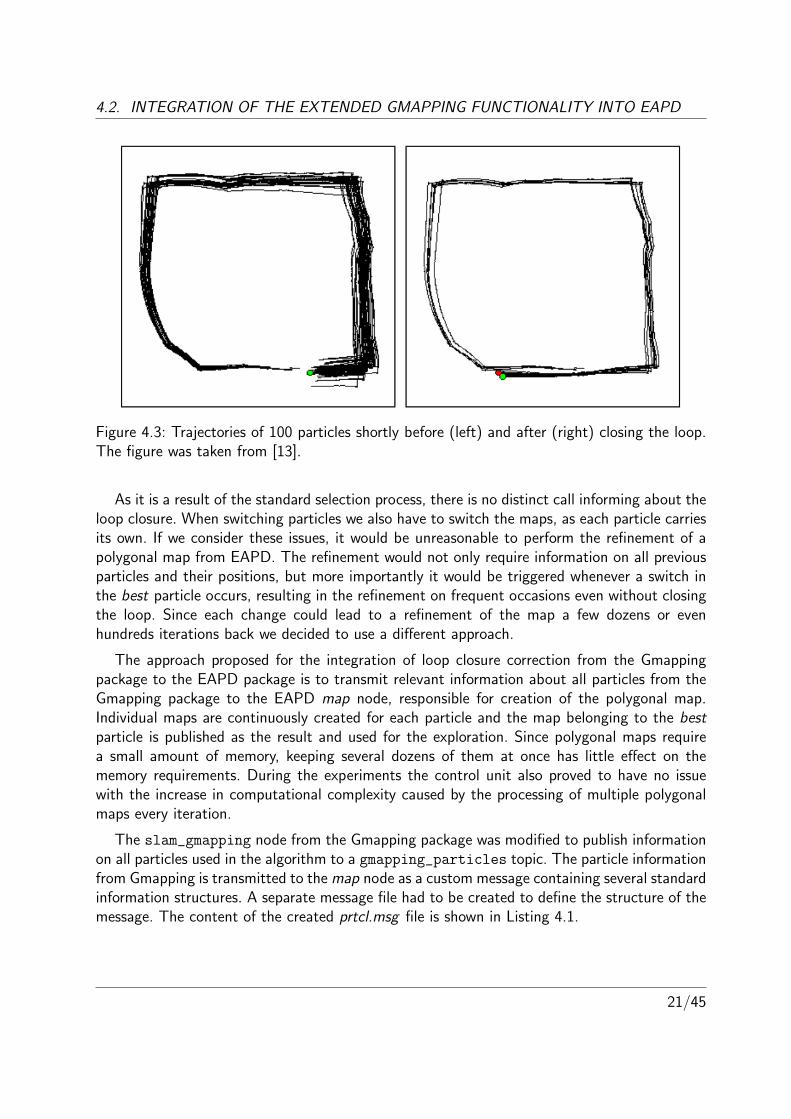
Gmapping uses scan matching to find a correlation between measurements projected fromthe pose of the corresponding particle and the posterior map in its surroundings. The bettermatching particles are favored during the creation of the new generation, reducing the uncer-tainty about robot’s position. Figure 4.3 visualizes trajectories of particles shortly before andafter it came in the vicinity of previously taken data.

As specified in section 2.1.1, the importance weighing also results in a selection of the bestparticle. It’s position is then published as the new position of the robot, together with it’s map.

4.2 Integration of the extended Gmapping functionalityinto EAPD

While Gmapping has the advantage of a path correction after a loop closure, the correctionitself is a part of a standard particle weighting and selection process. The loop closure usuallyleads to a switch of the best particle or eventually to the resampling of particles.

20/45

4.2. INTEGRATION OF THE EXTENDED GMAPPING FUNCTIONALITY INTO EAPD

Figure 4.3: Trajectories of 100 particles shortly before (left) and after (right) closing the loop.The figure was taken from [13].

As it is a result of the standard selection process, there is no distinct call informing about theloop closure. When switching particles we also have to switch the maps, as each particle carriesits own. If we consider these issues, it would be unreasonable to perform the refinement of apolygonal map from EAPD. The refinement would not only require information on all previousparticles and their positions, but more importantly it would be triggered whenever a switch inthe best particle occurs, resulting in the refinement on frequent occasions even without closingthe loop. Since each change could lead to a refinement of the map a few dozens or evenhundreds iterations back we decided to use a different approach.

The approach proposed for the integration of loop closure correction from the Gmappingpackage to the EAPD package is to transmit relevant information about all particles from theGmapping package to the EAPD map node, responsible for creation of the polygonal map.Individual maps are continuously created for each particle and the map belonging to the bestparticle is published as the result and used for the exploration. Since polygonal maps requirea small amount of memory, keeping several dozens of them at once has little effect on thememory requirements. During the experiments the control unit also proved to have no issuewith the increase in computational complexity caused by the processing of multiple polygonalmaps every iteration.

The slam_gmapping node from the Gmapping package was modified to publish informationon all particles used in the algorithm to a gmapping_particles topic. The particle informationfrom Gmapping is transmitted to the map node as a custom message containing several standardinformation structures. A separate message file had to be created to define the structure of themessage. The content of the created prtcl.msg file is shown in Listing 4.1.

21/45

4.3. IMPLEMENTATION OF POLYGONAL MAP REFINEMENT IN CASE OF LOOPCLOSURE DETECTION

Header header

geometry_msgs/Twist[] poses

int32[] p_index

sensor_msgs/LaserScan l_scan

int32 best_index

Listing 4.1: File prtcl.msg, defining a customized message

The necessary particle information contains a standard header used by ROS messages, anarray with particle positions in a form of a standard ROS Twist message, an array of indexescorresponding to particles from the previous generation, information on the best particle and alaser scan message corresponding to this specific batch of particles.

The map node in the EAPD package was modified to subscribe to the /gmapping_particlestopic and process the new information in the following manner:

1. When a new message in the /gmapping_particles topic is detected a ParticleSet func-tion is triggered to process the new batch of particles.

2. The node keeps a memory of maps, created by the previous batch of particles. When anew particle is processed, the algorithm takes corresponding map, based on the previousindex number from the message, and updates the map using the particle position andlaser scan information.

3. When all the new maps are created, the algorithm selects the map belonging to thebest particle, based on the best_index from the message file, and publishes it on the/map_global topic.

A gmapping_particles parameter was integrated into the EAPD package. This parameteris used to specify the number of particles expected by the map node and also works as a switchbetween the functionality following all the Gmapping particles and the original functionality ofthe EAPD package using the transformation topic for position information triggered by a newlypublished laser scan message. The parameter is optional and set to 0 as default, forcing theoriginal functionality of the EAPD package.

4.3 Implementation of polygonal map refinement in caseof loop closure detection

The integration of the loop closure functionality with the use of Gmapping is specific toparticle based SLAM algorithms. If the EAPD package is used with different SLAM or loopclosure detection algorithms a more general solution is desired.

A new ”loop” node was integrated in the EAPD algorithm as a part of this thesis. The loopnode is based on the original map node and provides the same functionality, extended by an

22/45

4.3. IMPLEMENTATION OF POLYGONAL MAP REFINEMENT IN CASE OF LOOPCLOSURE DETECTION

option for a map refinement. The loop node was written as a proposed solution to the maprefinement problem. A visualization of the desired map refinement functionality can be seen inFig. 4.4. The experiments proving the functionality of the node are described in section 5.

Figure 4.4: A visualization of a map refinement. The initially incorrect path is visualized in redcolor, as well as the section of the map generated along the incorrect path. The green colorrepresents the corrected path and the newly refined map section. The dashed arrow representsthe path correction.

The loop node saves previous positions of the robot and all measurements taken by thelaser rangefinder, and uses it for the map refinement. The refinement is triggered by an outsidemessage on the /map_correction topic, where a customized message contains information onthe loop closure correction.

As described in figure 4.2, the robot travels through the environment, circles back to apreviously visited position and has to adjust its pose information using a loop closure correction

23/45

4.3. IMPLEMENTATION OF POLYGONAL MAP REFINEMENT IN CASE OF LOOPCLOSURE DETECTION

value. The loop closer correction value indicates the difference between the current positionand the previous position. Our initial assumption is that the /map_correction topic publishedfrom a ”loop detection” node provides information on the previous and current positions andthe correction value.

The initial functionality of the loop node is the same as the map node. When the nodereceives a message from the /laser_scan topic it processes the scan into the polygonal map,and saves the laser scan message and the current position during the process. For conve-nience the node also saves every X-th map. The number can be changed using a newly addedmap_frequency parametr, set to 50 as default. Keeping ”checkpoints”, the program doesn’thave to rebuild the whole map, but can more or less accurately refine only the part affected bythe loop closure.

The refinement process can be described in 3 steps.

1. Trigger: The loop node receives a message from the /map_correction topic containingthe previous position, current position and the loop closure correction. This triggers aPathChange function.

2. Path change: The function iterates through the path of the robot, starting with theprevious position. The path correction contains a difference between the current positionand the desired position of the robot in x, y coordinates and the angle correction yawvalue.

The correction values (xc, yc and yawc) are iteratively distributed between individualposition changes. Each position Pi can be represented by its coordinates xi, yi and yawi.For each position touple < Pi, Pi+1 >, the additional change is proportional to the ratiobetween the difference in positions and the total movement over the loop.

These vales are computed individually for each coordinate. An example of a change inthe x coordinate of position Pi can be computed using the total movement over the loopin the x coordinate difftotal =

∑currentj=1 |xj − xj−1| described by a sum of changes in the

x coordinate from the beginning of the loop till the current position. The change of themovement can be computed using the following equation:

diffi =xc(xi − xi−1)

difftotal(4.1)

The new x coordinate for the position is then computed as:

xi = xi +i∑

j=1

diffj (4.2)

3. Map refinement: The last map saved before the starting position of the loop is selectedfor the refinement. The map is updated iteratively using the newly modified path of therobot and saved laser scan measurements.

24/45

Chapter 5

Experimental results

The task of the EAPD framework is to explore its surroundings and create a polygonalmap of the environment. A series of experiments was performed to confirm the functionalityof implemented algorithms. A common setup and hardware is described in the first part ofthe chapter. The rest of the chapter is dedicated to specific setup, experiments and results ofindividual implementations.

During the process of the implementation and debugging of the algorithms the Stage simula-tor [15] was used extensively. The final experiments were executed with a real robot, to confirmthe functionality in a real environment.

The Stage simulator[15] was used extensively during the process of the implementation anddebugging of the algorithms.

5.1 Hardware

The experiments were performed using a TurtleBot mobile robot equipped with the SICKLMS 111-10100 laser rangefinder. All the algorithms and computations were run on an INTELNUC5i5RYK control unit.

5.1.1 TurtleBot

TurtleBot with the Kobuki robot base is a popular platform for researchers and students.The Turtlebot meta package in ROS provides basic drivers for running and using the robot.The robot provides odometry information and data from tactile sensors placed at the front.Robot’s movement is supported by two differential motors that can be controlled from the ROSinterface. The robot is equipped with its own power source, making it a self sufficient unit, andcan be connected to the control unit with a single USB cable.

25/45

5.1. HARDWARE

A hardware mounting kit that can be attached to the base is provided with the robot,supporting the attachment of additional equipment(i.e. sensors or a control unit). Althoughthe mounting kit can be freely customized a few modifications were made to support thelaser rangefinder. The rangefinder was mounted to the construction and placed approximately15 centimeters above ground. The low placement was chosen to prevent the sensor from theoverlooking of obstacles.

An external 12V battery providing power supply for the laser and the control unit is fixedto the mounting kit by customized 3D printed holders. The battery was attached to a simpleOn/Off switch and connectors for the laser and the control unit.

Both the laser and the battery had to be properly fixed. Their weights are considerably heavyin comparison to the robot and an improper placement could affect the overall movement of therobot or even result in a system failure. The TurtleBot mounted with the rest of the equipmentcan be seen in Fig. 5.1.

Figure 5.1: The TurtleBot mobile robot equipped with the laser rangefinder and the controlunit, connected to a external battery.

26/45

5.1. HARDWARE

5.1.2 LaserRangefinder

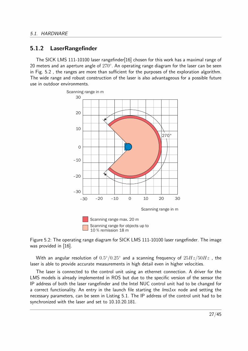
The SICK LMS 111-10100 laser rangefinder[16] chosen for this work has a maximal range of20 meters and an aperture angle of 270◦. An operating range diagram for the laser can be seenin Fig. 5.2 , the ranges are more than sufficient for the purposes of the exploration algorithm.The wide range and robust construction of the laser is also advantageous for a possible futureuse in outdoor environments.

Figure 5.2: The operating range diagram for SICK LMS 111-10100 laser rangefinder. The imagewas provided in [16].

With an angular resolution of 0.5◦/0.25◦ and a scanning frequency of 25Hz/50Hz , thelaser is able to provide accurate measurements in high detail even in higher velocities.

The laser is connected to the control unit using an ethernet connection. A driver for theLMS models is already implemented in ROS but due to the specific version of the sensor theIP address of both the laser rangefinder and the Intel NUC control unit had to be changed fora correct functionality. An entry in the launch file starting the lms1xx node and setting thenecessary parameters, can be seen in Listing 5.1. The IP address of the control unit had to besynchronized with the laser and set to 10.10.20.181.

27/45

5.2. ENVIRONMENT

<node pkg="lms1xx" name="lms1xx" type="LMS1xx_node" output="screen">

<param name="host" value="10.10.20.180" />

<param name="frame_id" type="string" value="/scan" />

</node>

Listing 5.1: lms1xx driver section in the launch file.

The sensor is mounted to the robot in an upside-down position, this enables the laser to getmeasurements from a position, which is relatively close to the ground (15 cm), allowing a properresponse for most of the obstacles faced during the exploration. There is a possibility to setthe position of the laser upside down using the transformation library in ROS, however not allpackages are compatible with these settings, therefore a separate node that would rewrite themeasurements had to be written. The laser_switch node was written to revers measurementstaken by the sensor. The node could also be used to trim the measurements in case the robotsees itself or to remove invalid values, coming from the measurements. The source code of thelaser_switch node is available in the CD, provided with this thesis.

5.1.3 Intel NUC mini computer

The INTEL NUC5i5RYK mini computer uses a dual core 1.6 GHz processor, 16 GB RAM andis running the Ubuntu 14.04 operation system. The unit offers wi-fi and bluetooth connection,together with and ethernet connection and 4 USB 3.0 ports. The version of ROS used is theIndigo version.

5.2 Environment

The experiments with a real robot should reveal possible issues with noise in sensory data,low precision of the localization algorithm or the ability of the exploration algorithm to dealwith an external movement in the environment, i.e. passers-by or opened doors.

Three sets of functionalities were tested, the integration of Gmapping as a SLAM algo-rithm with the EAPD framework, the integration of extended Gmapping functionality and therefinement of the polygonal map. The experiments were based on a common setup in boththe software parameters and hardware settings, apart for the parameters specific for individualfunctionalities.

The EAPD parameters include parameters for map dexterity and visualization, snd param-eters for robot’s navigation, and several others. The main parameters are the robot_radius

influencing the navigation, the poly_epsilon parameter setting the detail in which the mapwill be kept and the map_laser_range which marks any measurements further than its distanceas frontiers. These parameters were set to values 0.2, 0.05 and 5.0 respectively (the values arein meters). The params_set.yaml file used for the setting of parameters is included on theCD provided with this thesis.

28/45

5.2. ENVIRONMENT

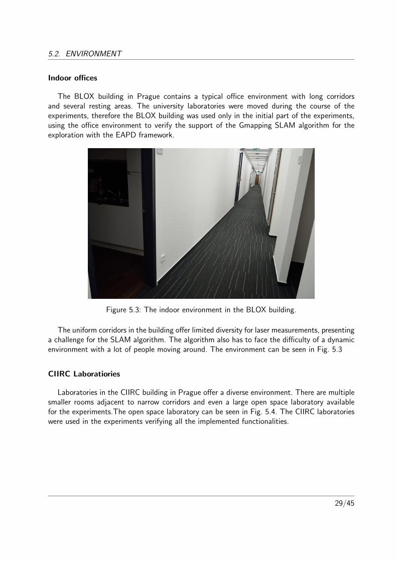
Indoor offices

The BLOX building in Prague contains a typical office environment with long corridorsand several resting areas. The university laboratories were moved during the course of theexperiments, therefore the BLOX building was used only in the initial part of the experiments,using the office environment to verify the support of the Gmapping SLAM algorithm for theexploration with the EAPD framework.

Figure 5.3: The indoor environment in the BLOX building.

The uniform corridors in the building offer limited diversity for laser measurements, presentinga challenge for the SLAM algorithm. The algorithm also has to face the difficulty of a dynamicenvironment with a lot of people moving around. The environment can be seen in Fig. 5.3

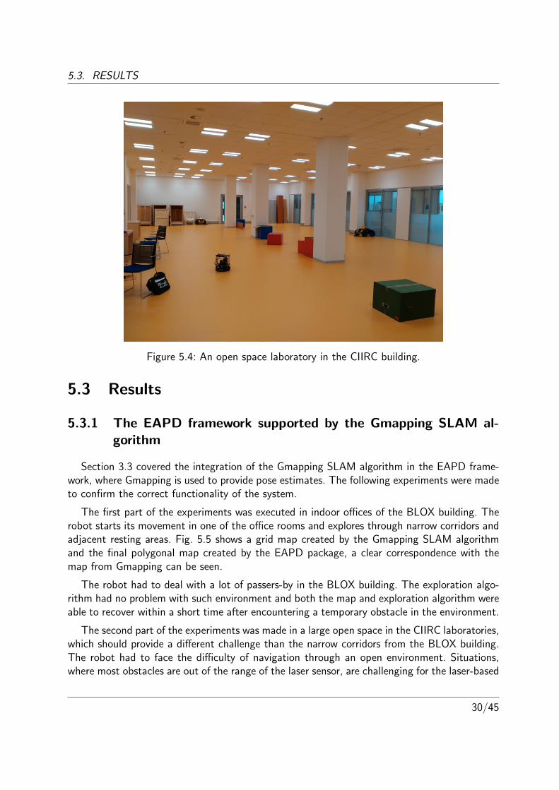
CIIRC Laboratiories

Laboratories in the CIIRC building in Prague offer a diverse environment. There are multiplesmaller rooms adjacent to narrow corridors and even a large open space laboratory availablefor the experiments.The open space laboratory can be seen in Fig. 5.4. The CIIRC laboratorieswere used in the experiments verifying all the implemented functionalities.

29/45

5.3. RESULTS

Figure 5.4: An open space laboratory in the CIIRC building.

5.3 Results

5.3.1 The EAPD framework supported by the Gmapping SLAM al-gorithm

Section 3.3 covered the integration of the Gmapping SLAM algorithm in the EAPD frame-work, where Gmapping is used to provide pose estimates. The following experiments were madeto confirm the correct functionality of the system.

The first part of the experiments was executed in indoor offices of the BLOX building. Therobot starts its movement in one of the office rooms and explores through narrow corridors andadjacent resting areas. Fig. 5.5 shows a grid map created by the Gmapping SLAM algorithmand the final polygonal map created by the EAPD package, a clear correspondence with themap from Gmapping can be seen.

The robot had to deal with a lot of passers-by in the BLOX building. The exploration algo-rithm had no problem with such environment and both the map and exploration algorithm wereable to recover within a short time after encountering a temporary obstacle in the environment.

The second part of the experiments was made in a large open space in the CIIRC laboratories,which should provide a different challenge than the narrow corridors from the BLOX building.The robot had to face the difficulty of navigation through an open environment. Situations,where most obstacles are out of the range of the laser sensor, are challenging for the laser-based

30/45

5.3. RESULTS

Figure 5.5: A map of the BLOX building created by the exploration algorithm. The Gmappingoccupancy grid map is on the left and the polygonal map created by EAPD is on the right.

SLAM algorithm and the robot has an increased need for a precise odometry information. Fig.5.6 presents the created maps from Gmapping and EAPD.

The functionality of the system is apparent, as the exploration was fully autonomous andthe robot was able to create a model of the environment in both buildings.

Figure 5.6: A map of the CIIRC laboratory created by the exploration algorithm. The Gmappingoccupancy grid map is on the left and the polygonal map created by EAPD is on the right.

31/45

5.3. RESULTS

5.3.2 The EAPD framework with the use of the extended Gmappingfunctionality

Section 4.2 presents the integration of the extended Gmapping functionality into the EAPDpackage. The Gmapping package was modified to publish specific information on all particlesallowing the EAPD package to synchronize with the SLAM algorithm. This synchronizationallows the adaptation to the changes in the best particle described at page 5. Experimentstesting this functionality are presented here.

Although the SLAM algorithm proved to be functional during the previous experiments,its connection with the exploration package was limited only to the estimates of the currentposition. This resulted in the inability of the exploration algorithm to properly react to thechanges made by the Gmapping SLAM during a switch between particles. Fig. 5.7 presents asituation shortly before and after the switch in the best particle. The image on the left presentsthe state prior to the particle switch. The image on the right shows an incoherency in mapsproduced by the algorithms, caused by a change in the best particle.

Figure 5.7: An overlay of the polygonal map and the grid map, before(left) and after(right) aswitch in the best particle in the Gmapping SLAM algorithm. The situation occurred duringthe experiments testing the slam functionality, connected with the creation of the map in Fig.5.5.

The Gmapping algorithm processes all particles during the process, it has already assimilateda full path of the particle leading to the current position and only switched between the particlesand their map representations. However the EAPD algorithm has been following a differentparticle up to the point where the switch occured and received only the resulting change inposition at the time of the switch, therefore the map created prior to the switch occurrencefollows a different path than the path of the current best particle.

32/45

5.3. RESULTS

Figure 5.8: An overlay of the polygonal map and the grid map, before(top) and after(bottom)a switch in the best particle in the Gmapping SLAM algorithm. A green grid has been addedto emphasize the shift in the structure of the maps.

33/45

5.3. RESULTS

The modifications made in Section 4.2 were initially proposed to integrate Gmapping loopclosure functionality, but since the functionality in Gmapping projects itself in the selectionof the best particle, the approach had to be changed and the EAPD framework had to beextended to support switches between the particles. Experiments testing the new functionalitywere performed in CIIRC laboratories and are focused on the proper functionality during aparticle switch.

Fig. 5.8 presents the situation shortly before and after the switch in the best particle. As canbe seen in the figure, the structure of both maps shifted in reaction to the switch. The mapsare fully aligned after the shift, which proves the correct functionality of the implementation.

Although this new approach prevents discontinuities in the polygonal map and supports theloop closure functionality from Gmapping, the new implementation has two downsides to it:

• The first one is the limitation on the visualization functionality for the map. Until nowthe map was visualized incrementally, however with the new changes the visualization isswitching between complete map representations. For a correct visualization of the mapunder the new functionality, the clean_map map parameter in EAPD had to be set astrue. The setting doesn’t have any influence on the exploration algorithm itself but itinfluences the visualization of the map, forcing it to disregard more recent measurementsof a previously integrated area.

• The second downside is the increased demand on the CPU usage. The map node hasto process dozens of maps during one iteration instead of the one map in the originalfunctionality. The number of maps depends on the number of particles, our approach used30 particles - the default setting of the Gmapping algorithm. Although the explorationprocess was still fluent, the CPU usage increased to 5 times of the original and the memoryrequirements tripled. The Process monitor plugin in the RQT development tool was usedto monitor the CPU and memory usage.

5.3.3 Map refinement with a separate loop node

The integration of the map refinement into the EAPD algorithm is covered in Section 4.3.A separate loop node derived from the map node was written to provide the functionality torefine a section of a map according to specifications received from an outside source. The nodewas initially intended for situations regarding a loop closure, but due to the character of thefinal implementation the functionality is suitable for a general map refinement and the namewas therefore changed to the refinement node in the final version of the framework.

The node as it is doesn’t affect the overall functionality of the EAPD package and is providedwith the package solely for the purpose of possible future uses in situations where a refinementof the polygonal map is desired (i.e. the aforementioned loop closure). To confirm the correctfunctionality of the refinement, the original map node was substituted with the loop node anda series of experiments was executed with a real robot in this setup.

34/45

5.3. RESULTS

Figure 5.9: An overlay of the polygonal map and the grid map, before(left) and after(right) therefinement of the polygonal map.

35/45

5.4. DISCUSSION OF THE RESULTS

As we currently don’t have any working slam algorithm that would be capable of producinga sufficient refinement information, a separate closure_detection node was written to sim-ulate both the deviation in robot’s position and the map refinement message containing theinformation needed for the loop node.

The synchronization of the closure_detection node and the loop node through the maprefinement message is one of the critical parts in the solution and has to be customized whenused. In our example we use a simple synchronization through a counter variable determiningthe number of the laser messages received and their matching positions.

We use the closure_detection node to provide fake position messages to the loop node.The fake positions are created by shifting the correct positions received from Gmapping in oneof the coordinates, in our case it is the x coordinate. At a specific time, the position starts toshift and after a hundred iterations a refinement message is send with the accumulated errorin the position. The message carries the start and the end point of the deviation in the form ofthe appropriate counter values, and the correction value.

The results of the map refinement can be seen in Fig. 5.9 presenting the polygonal mapcreated with the use of deviated positions and the same map after the refinement. After therefinement, the polygonal map aligned with the original map created by the Gmapping package.

The refinement processed only the last 100 positions. The refinement was processed in real-time and the additional CPU usage didn’t have a specific effect on the exploration process.The refinement of 100 positions and laser scans was processed in approximately 1 second, therewas a slight variation in the time with every executed experiment. The peak in the CPU usagelasted less then a second, and regretfully the current monitoring packages available in ROS wereunable to provide more specific statistics for such a short time. Even though the refinementwas processed in real-time, we can assume that the usage with a significantly larger segment ofthe map could have a higher demand on the computational complexity. In such situations thenode can easily be modified to work offline with recorded data.

5.4 Discussion of the results

A mobile robot suitable for exploration was set up with a laser rangefinder and a control unit.The functionality of implemented algorithms was successfully tested during the experiments,individual comments to each functionality are listed bellow.

1. The EAPD framework supported by the Gmapping SLAM algorithm: The inte-gration of the SLAM algorithm with EAPD was successful. The robot properly exploredits surroundings and created a polygonal map representing the environment.

However due to the nature of the particle filter based SLAM algorithm the final map wasaffected by the SLAM algorithm switching between individual particles. As can be seenin Fig. 5.7 the situation caused a discontinuity in the polygonal map.

36/45

5.4. DISCUSSION OF THE RESULTS

2. The EAPD framework with the use of extended Gmapping functionality: Theintegration of information on particles from Gmapping into the EAPD framework suc-cessfully solved both the problem caused by a particle switch, and the integration ofGmapping’s loop closure detection and map refinement functionality.

However the computational requirements of the new version of the map node were sev-eral times higher than that of the original solution, especially during a particle switchoccurrence. The rise is caused by the increase in the number of processed maps.

3. Map refinement with a separate loop node: The refinement of the polygonal map wasimplemented in a separate node, but it can be freely used in a place of the original mapnode. A crucial part for the refinement process is the synchronization of the refinementalgorithm and the algorithm responsible for providing the request for the refinement.

The refinement can processed reasonably large segments of map in real-time and can bemodified to provide offline refinement if needed.

37/45

Chapter 6

Conclusion

The goal of this thesis was to set up a hardware solution with a real mobile robot equippedwith a laser rangefinder for the use with the EAPD exploration framework, integrate a SLAMlibrary into EAPD and design and implement loop closure and map refinement methods for apolygonal map generated by the EAPD framework. The implemented functionalities were testedin various environments with a mobile robot.

A hardware setup was implemented using the Kobuki robot base with the TurtleBot roboticpackage. The robot is controlled by the Intel NUC mini computer and uses the SICK LMS111-10100 laser rangefinder to navigate through the environment. The control unit and laserwere mounted to the robot base and connected to an external battery allowing for over 60minutes of usage.

The Gmapping SLAM library was selected as a reliable provider of position estimates andintegrated into the EAPD framework, allowing the exploration with the use of a laser rangefinder.The functionality was tested with the Kobuki robot in several different environments and theexploration framework supported by the SLAM library proved to achieve decent results.

Two approaches were chosen for the implementation of the loop closure and map refinementfunctionality. The first method is connected to the particle filter based SLAM algorithm in theGmapping library. The second method was designed as a general map refinement, which couldbe used in a wider scope of applications.

A method to synchronize the particle filter functionality with the EAPD framework wasproposed and implemented. The newly proposed method should be suitable for the use withmost particle filter based SLAM algorithms. The method can remove negative impact of jumpsin the estimated position caused by a switch in the best particle from the SLAM algorithm,improving the precision of the created polygonal map. The method also supports the innate loopclosure functionality of the Gmapping library. The downside is that the new implementation hashigher computational requirements than the original mapping process.

A method for a general map refinement was proposed and implemented. Since the approachto map refinement is different than for the first method, a separate ROS node was implemented

38/45

for the second approach. The new node is derived from the original map node responsible forthe creation of a polygonal map in the EAPD framework, and can be freely used in place of theoriginal map node.

The functionality of the refinement was successfully tested with a real robot. The refinementcan be executed in real-time during the exploration on moderately large segments of the map.The refinement can be synchronized with an outside loop closure detection algorithm or used inother situations where a map refinement is required, however the synchronization in such casesis a crucial part of the implementation and has to be handled with extra care.

So far, the EAPD framework was only tested with external SLAM libraries. This work usesthe Gmapping SLAM library and T.Juchelka[1] used the EAPD framework together with theRTAB-Map library. This part of the solution offers an opportunity for improvement, since theEAPD framework creates its own polygonal map of the environment. An implementation of aSLAM algorithm using the polygonal map as its base could simplify the solution, as there wouldbe no need to create an additional map solely for the SLAM algorithm.

39/45

BIBLIOGRAPHY

Bibliography

[1] T. Juchelka, Exploration algorithms in a polygonal domain. CTU in Prague, FEL, Dept. ofCybernetics, 2012.

[2] The official website of the Robot Operating System(ROS).http://www.ros.org

[3] V. Lhotsky, An Integrated Approach to Multi-Robot Exploration of an Unknown Space.CTU in Prague, FEL, Dept. of Cybernetics, 2016.

[4] The official website of the OpenSLAM project.https://www.openslam.org/

[5] Giorgio Grisetti, Cyrill Stachniss, Wolfram Burgard, Improving Grid-based SLAM with Rao-Blackwellized Particle Filters by Adaptive Proposals and Selective Resampling. In Proc. ofthe IEEE International Conference on Robotics and Automation (ICRA), 2005.

[6] Wikimedia Commons, the free media repository.https://commons.wikimedia.org/wiki/File:Particle2dmotion.svg

[7] Giorgio Grisetti, Cyrill Stachniss, Wolfram Burgard, Improved Techniques for Grid Mappingwith Rao-Blackwellized Particle Filters. IEEE Transactions on Robotics, Volume 23, pages34-46, 2007.

[8] Matıas Nitsche, Pablo de Cristoforis, Miroslav Kulich and Karel Kosnar, Hybrid Mapping forAutonomous Mobile Robot Exploration. Intelligent Data Acquisition and Advanced Com-puting Systems (IDAACS), 2011.

[9] J. W. Durham and F. Bullo, Smooth Nearness-Diagram navigation. Intelligent Robots andSystems, 2008.

[10] A. Johnson, Clipper - an open source freeware library for clipping and offsetting lines andpolygons. Available from http://www.angusj.com/delphi/clipper.php.

[11] Jens-Steffen Gutmann and Kurt Konolige, Incremental Mapping of Large Cyclic Environ-ments. Computational Intelligence in Robotics and Automation, 1999

40/45

BIBLIOGRAPHY

[12] Paul Newman and Kin Ho, SLAM- Loop Closing with Visually Salient Features. ICRA,2005

[13] Dirk Hahnel, Wolfram Burgard , DIeter Fox and Sebastian Thrun, An Efficient FastSLAMAlgorithm for Generating Maps of Large-Scale Cyclic Environments from Raw Laser RangeMeasurements. IEEE International Conference on Intelligent Robots and Systems, (Vol. 1,pp. 206-211), 2003.

[14] Brian Williams, Mark Cummins, Jose Neira, Paul Newman, Ian Reid and Juan Tardos,A comparison of loop closing techniques in monocular SLAM. Robotics and AutonomousSystems, 2009.

[15] Richard Vaughan, Massively Multiple Robot Simulations in Stage. Swarm Intelligence 2(2-4):189-208, 2008.

[16] The official website of the Sick company.https://www.sick.com

41/45

LIST OF FIGURES

List of Figures

2.1 The left picture presents a visualization of particle distribution after a few itera-tions based on odometry. The right picture describes particle distribution basedon odometry and laser measurements in several specific environments. Pictureswere taken from [6] and [5]. . . . . . . . . . . . . . . . . . . . . . . . . . . . 4

2.2 A diagram describing the exploration process. . . . . . . . . . . . . . . . . . . 6

2.3 A visualization of an occupancy grid map. Frontiers are marked in blue color,obstacles are black and the unexplored area is gray. The robot is represented bya green circle. . . . . . . . . . . . . . . . . . . . . . . . . . . . . . . . . . . 7

2.4 A visualization of an inflated map from Fig. 2.3. The original obstacles wereinflated by the size of the robot radius (marked with a red color) and the robotrepresentation has been replaced with a single point in the C-space. . . . . . . 7

2.5 A visualization of a topological map overlay over a metric map. The area nodesare represented by blue circles and the gateway nodes are represented by yellowrectangles. . . . . . . . . . . . . . . . . . . . . . . . . . . . . . . . . . . . . 9

2.6 A polygonal representation of the map from Fig. 2.3. The obstacles are markedin red color and the frontiers are marked blue. . . . . . . . . . . . . . . . . . 10

3.1 A visualization of transformation frames in ROS. The image presents connectionsbetween individual coordinate frames. . . . . . . . . . . . . . . . . . . . . . . 12

3.2 An example an offset polygonal map. . . . . . . . . . . . . . . . . . . . . . . 14

3.3 An example of a visibility graph. . . . . . . . . . . . . . . . . . . . . . . . . . 14

4.1 A visualization of a loop closure. . . . . . . . . . . . . . . . . . . . . . . . . 18

4.2 A close-up of figure 4.1. The loop closure correction is marked with a blue arrow.The correction values x, y and yaw are depicted in the visualization. . . . . . . 18

4.3 Trajectories of 100 particles shortly before (left) and after (right) closing theloop. The figure was taken from [13]. . . . . . . . . . . . . . . . . . . . . . . 21

42/45

LIST OF FIGURES

4.4 A visualization of a map refinement. The initially incorrect path is visualizedin red color, as well as the section of the map generated along the incorrectpath. The green color represents the corrected path and the newly refined mapsection. The dashed arrow represents the path correction. . . . . . . . . . . . 23

5.1 The TurtleBot mobile robot equipped with the laser rangefinder and the controlunit, connected to a external battery. . . . . . . . . . . . . . . . . . . . . . . 26

5.2 The operating range diagram for SICK LMS 111-10100 laser rangefinder. Theimage was provided in [16]. . . . . . . . . . . . . . . . . . . . . . . . . . . . 27

5.3 The indoor environment in the BLOX building. . . . . . . . . . . . . . . . . . 29

5.4 An open space laboratory in the CIIRC building. . . . . . . . . . . . . . . . . 30

5.5 A map of the BLOX building created by the exploration algorithm. The Gmap-ping occupancy grid map is on the left and the polygonal map created by EAPDis on the right. . . . . . . . . . . . . . . . . . . . . . . . . . . . . . . . . . . 31

5.6 A map of the CIIRC laboratory created by the exploration algorithm. The Gmap-ping occupancy grid map is on the left and the polygonal map created by EAPDis on the right. . . . . . . . . . . . . . . . . . . . . . . . . . . . . . . . . . . 31

5.7 An overlay of the polygonal map and the grid map, before(left) and after(right)a switch in the best particle in the Gmapping SLAM algorithm. The situationoccurred during the experiments testing the slam functionality, connected withthe creation of the map in Fig. 5.5. . . . . . . . . . . . . . . . . . . . . . . . 32

5.8 An overlay of the polygonal map and the grid map, before(top) and after(bottom)a switch in the best particle in the Gmapping SLAM algorithm. A green gridhas been added to emphasize the shift in the structure of the maps. . . . . . . 33

5.9 An overlay of the polygonal map and the grid map, before(left) and after(right)the refinement of the polygonal map. . . . . . . . . . . . . . . . . . . . . . . 35

43/45

LIST OF TABLES

List of Tables

6.1 CD Content . . . . . . . . . . . . . . . . . . . . . . . . . . . . . . . . . . . 45

44/45

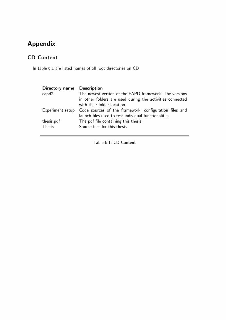
Appendix

CD Content

In table 6.1 are listed names of all root directories on CD

Directory name Descriptioneapd2 The newest version of the EAPD framework. The versions

in other folders are used during the activities connectedwith their folder location.

Experiment setup Code sources of the framework, configuration files andlaunch files used to test individual functionalities.

thesis.pdf The pdf file containing this thesis.Thesis Source files for this thesis.

Table 6.1: CD Content