
EXPLORATION By Brandon Kerry Eames · A FINITE DOMAIN MODEL FOR DESIGN SPACE EXPLORATION By Brandon...
205
A FINITE DOMAIN MODEL FOR DESIGN SPACE EXPLORATION By Brandon Kerry Eames Dissertation Submitted to the Faculty of the Graduate School of Vanderbilt University in partial fulfillment of the requirements for the degree of DOCTOR OF PHILOSOPHY in Electrical Engineering May, 2005 Nashville, Tennessee Approved: Professor Janos Sztipanovits Professor Gabor Karsai Doctor Theodore A. Bapty Professor Gautam Biswas Doctor Ben A. Abbott Doctor Sandeep K. Neema
Transcript of EXPLORATION By Brandon Kerry Eames · A FINITE DOMAIN MODEL FOR DESIGN SPACE EXPLORATION By Brandon...

A FINITE DOMAIN MODEL
FOR DESIGN SPACE
EXPLORATION
By
Brandon Kerry Eames
Dissertation
Submitted to the Faculty of the
Graduate School of Vanderbilt University
in partial fulfillment of the requirements
for the degree of
DOCTOR OF PHILOSOPHY
in
Electrical Engineering
May, 2005
Nashville, Tennessee
Approved:
Professor Janos Sztipanovits
Professor Gabor Karsai
Doctor Theodore A. Bapty
Professor Gautam Biswas
Doctor Ben A. Abbott
Doctor Sandeep K. Neema

Copyright © 2005 by Brandon Kerry Eames
All Rights Reserved

In memory of my father,
Oliver Dean Eames
June 18, 1948 – February 10, 2005
iii

ACKNOWLEDGEMENTS
I would be truly ungrateful without acknowledging the influence, help, guidance and support
from several sources. First and foremost, I thank my wife, Natalie, for her constant love and
companionship. Her unwavering patience and support, not only through six years of graduate
school, but throughout our married life has inspired and sustained me during this journey. I
know no words to express my humble gratitude, admiration and devotion to her. I also thank my
children, Karissa Rose and Warner Andrew. Their enthusiasm and loving smiles erase the
deepest of frustrations. I acknowledge the love and support of my parents, who are largely
responsible for my entrance into an academic career. To my wife’s parents, thank you for your
support of us and our children albeit over a great distance.
I wish to thank the members of my committee for their involvement in this research. To my
advisor, Professor Janos Sztipanovits, thank you for having confidence in my work when I did
not, and for sharing your vision, but leaving to me the joy of discovery. To Dr. Ted Bapty, I am
very grateful for the opportunity to have worked with you for several years at ISIS. With your
patient mentoring style, I felt I was treated as your colleague, not just as a student. Thank you
for giving me the opportunity to learn the ropes as a researcher. Trips to PI meetings were
always an adventure. To Dr. Sandeep Neema, I owe you a great deal. Much of the work in this
dissertation draws on your research; I am very grateful not only for the time and attention you
gave this research, but for your friendship as well. To Dr. Gabor Karsai, thanks for being
involved in my graduate school career, and for the advice on my future as a faculty member. To
Dr. Gautam Biswas, thank you for teaching a great class on modeling and for encouraging me in
my future career in academics. To Dr. Ben Abbott, thank you for sparking my interest in
embedded systems while at Utah State, and for getting me interested in graduate school. Your
constant insistence that I not settle in anything I do has been a source of inspiration at times of
weakness.
To everyone at the Institute for Software Integrated Systems (ISIS), both present and former
members, I am a better person for having known you. The friendships and memories I have
made here I will treasure throughout my life. Dr. Jon Sprinkle, thanks for the great times we had
with photography and vacations to Florida. Dr. James “Bubba” Davis, Dr. Akos Ledeczi, Dr.
Greg Nordstrom, Dr. Jason Scott, Dr. Gyula Simon, Zoltan Molnar, Gabor Pap, and so many
iv

others, I am grateful for your friendship and positive influence. To the present and former
graduate students at ISIS, Dr. Aditya Agrawal, Steve Nordstrom, Kumar Chhokra, Dr. Jeff Gray,
Abdullah Sowayan, Shweta Shetty, Di Yao, Shikha Ahuja, Brano Kusi, Robert Regal, and so
many others, thank you for being so accepting, and for creating a positive environment for
graduate studies. I wish to thank Dr. Sherif Abdelwahed for his help with the formal logic, and
David Hanak for help in learning the Mozart programming system. To the administration of
ISIS, Michele Codd and Lorene Morgan among others, you have made my time as a graduate
student not only bearable but enjoyable, through your supportive and congenial personalities. I
appreciate your tutelage in preparing me for the administrative side of my future academic
career.
I am very appreciative of the fellowship and friendship of the members of the West
Nashville Ward of the Church of Jesus Christ of Latter-day Saints. You have been family for the
last six years, and your willingness to serve at a moment’s notice is inspiring. Thank you for
being there for us in our times of need.
Finally, I would like to gratefully acknowledge the financial support for this research. This
work has been partially supported by the National Science Foundation, the Defense Advanced
Research Projects Agency, the IBM Corporation, and by Vanderbilt University through a Harold
Sterling Vanderbilt Fellowship.
v

TABLE OF CONTENTS
Page
DEDICATION............................................................................................................................... iii
ACKNOWLEDGEMENTS........................................................................................................... iv
LIST OF FIGURES ....................................................................................................................... ix
LIST OF EQUATIONS ............................................................................................................... xiii
LIST OF ALGORITHMS..............................................................................................................xv
LIST OF ABBREVIATIONS..................................................................................................... xvii
Chapter
I. INTRODUCTION ...............................................................................................................1
Embedded System Overview ..........................................................................................2 Mathematics of System Design.......................................................................................3
Point Design vs. Design Space ..................................................................................4 Design Space Exploration .........................................................................................4
II. BACKGROUND .................................................................................................................8
Mixed Integer Linear Programming................................................................................8 Synthesis of ASIC Applications using MILP..........................................................10 Partitioning FPGA-based Applications using MILP...............................................12 Critique of MILP for Design Space Exploration.....................................................13 Linear Pseudo-Boolean Constraints ........................................................................13
Constraint Logic Programming.....................................................................................14 Finite Domain Constraints.......................................................................................16 Modeling System Synthesis with Finite Domain Constraints .................................18 Partial Assignment Technique.................................................................................21 Time-Triggered Software ........................................................................................22 Critique of Constraint Logic Programming.............................................................23
Combinatorial Search Heuristics ..................................................................................24 Simulated Annealing ...............................................................................................24 Evolutionary Algorithms .........................................................................................26 Critique of Combinatorial Search Heuristics...........................................................28
Branch and Bound in Real-Time Software Synthesis...................................................29 Minimum Required Speedup...................................................................................29 Component Allocation in the AIRES Toolkit .........................................................31 Critique of Branch and Bound.................................................................................32
Parameter-Based Design ...............................................................................................32 Platune .....................................................................................................................32 PICO ........................................................................................................................34 Evaluation of Parameter-Based Design...................................................................37
Design Space Exploration Tool (DESERT)..................................................................37
vi

DESERT Design Space Model................................................................................38 Symbolic Constraint Satisfaction ............................................................................41 Exploration of Adaptive Computing Systems .........................................................42 Critique of DESERT................................................................................................43
Design Space Exploration Summary and Critique........................................................44
III. A FINITE DOMAIN DESIGN SPACE MODEL .............................................................47
A Formal DESERT Design Space Model ...............................................................47 A Finite Domain Model for the AND-OR-LEAF Tree ................................................50
Implementation of the Finite Domain Model ..........................................................51 Simple Tree Example ..............................................................................................53
A Finite Domain Model for Design Space Properties ..................................................53 A Finite Domain Property Tree ...............................................................................54 Implementation of the Finite Domain Property Model ...........................................56 Simple Property Example........................................................................................60 Summary of the Finite Domain Property Model .....................................................62
A Finite Domain Model for OCL Constraints ..............................................................63 A Finite Domain Model for DESERT OCL Constraints.........................................64 DESERT OCL Constraints and Finite Domain Propagation...................................67 Summary of Finite Domain Model for OCL Constraints........................................67
Finite Domain Distribution ...........................................................................................67 Constraint Utilization and Finite Domain Search .........................................................72
Single-Solution and All-Solution Search ................................................................72 Constraint Utilization and Best-Solution Search.....................................................73 Performance Implications of Constraint Utilization................................................75 Summary of Constraint Utilization techniques .......................................................76
Summary of the Finite Domain Constraint Model for DESERT..................................76
IV. THE PROPERTY COMPOSITION LANGUAGE...........................................................78
Limitations in Modeling Property Composition ...........................................................78 The Property Composition Language ...........................................................................79
PCL Variables, Operations, Expressions and Statements .......................................80 Modularity in PCL: Properties and Functions.........................................................81 Tree Navigation .......................................................................................................82 List Iteration Functions............................................................................................83 Simple PCL Example: Area Property.....................................................................84
PCL Interpretation.........................................................................................................85 Expression Trees......................................................................................................85 Translation into Trees..............................................................................................87 From Expression Trees to Finite Domain Constraints ............................................95
PCL Modeling Example................................................................................................96 A Parameterized Component IP Library .................................................................97 Example Property Function: Adder Component .....................................................99 Design Composition through Exploration.............................................................101
Summary of PCL ........................................................................................................104 Expressiveness Limitations ...................................................................................104
vii

Implementation Inefficiency..................................................................................106 PCL Conclusions ...................................................................................................107
V. DESERTFD: AN INTEGRATED DESIGN SPACE EXPLORATION TOOL ............108
DESERT Toolflow......................................................................................................108 DESERT and Scalability .......................................................................................109
DesertFD Architecture and Implementation ...............................................................111 Implementation of Finite Domain Pruning............................................................112 Design Space Evaluation .......................................................................................113 The Oz Engine .......................................................................................................115 Mozart Implementation of Design Space Exploration ..........................................116 Alternative Implementation...................................................................................117 Integration and Hybridization................................................................................119 Constraint Set Partitioning.....................................................................................122 From BDD to Logic Function ...............................................................................123 Structural Redundancy ..........................................................................................128
Quantitative Scalability Analysis................................................................................129 Parametric Design Space Generation ....................................................................129 Representing Design Spaces: Propagators and Variables .....................................135 Over-, Under- and Critically-Constrained Spaces.................................................138 Width vs. Depth.....................................................................................................145 Experiment Evaluation and Applicability .............................................................149 Scalability Conclusions .........................................................................................150
Conclusions.................................................................................................................151
VI. CONCLUSIONS AND FUTURE WORK ......................................................................153
Summary of Findings..................................................................................................153 Future Work ................................................................................................................155
Design Space Modeling.........................................................................................155 Scalability Improvements with DesertFD .............................................................156 Solver Integration ..................................................................................................156 Embedding Exploration.........................................................................................157 Tool Integration .....................................................................................................158
Appendix
A. PCL LEXICAL ANALISYS SPECIFICATION.............................................................159
B. PCL CONTEXT-FREE GRAMMAR SPECIFICATION...............................................161
C. CASE STUDY: EMBEDDED AUTOMOTIVE SOFTWARE .....................................164
REFERENCES ............................................................................................................................183
viii
LIST OF FIGURES
Figure Page 1. A simple task graph .........................................................................................................20
2. Toolflow for design space exploration in PICO..............................................................35
3. UML representation of DESERT design space model....................................................39
4. UML representation of DESERT Properties ...................................................................40
5. UML representation of DESERT domains and domain membership .............................41
6. Oz code implementation of equation (20) .......................................................................52
7. Simple AND-OR-LEAF tree...........................................................................................53
8. Oz implementation of the select variables modeling the AND-OR-LEAF tree in Figure 6.................................................................................................................53
9. Oz implementation of the AND-node additive property composition relation defined in equation (24) .....................................................................................57
10. Blocking Oz implementation of the OR-node property composition relation defined in equation (23) .....................................................................................57
11. Oz implementation of OR node property composition, including redundant constraints to facilitate propagation................................................................59
12. Simple tree example, annotated with additive property AP ............................................60
13. Oz implementation of the simple property example of Figure 12...................................61
14. AND-OR-LEAF tree showing the results of finite domain propagation for the property AP..........................................................................................................62
15. Example DESERT OCL constraint, whose context is the node N4 from Figure 12..........................................................................................................................64
16. DESERT OCL constraint requiring the value of the context’s AP property not exceed 35 ....................................................................................................64
17. Oz implementation of the DESERT OCL constraint from Figure 15 .............................66
18. Oz implementation of the DESERT OCL constraint from Figure 16 .............................66
ix

19. Oz implementation of best-case ordering function for constraint utilization.........................................................................................................................75
20. Example PCL function modeling an additive property called area.................................85
21. Example PCL Expression tree modeling the PCL expression in equation .....................86
22. Parameterized adder component......................................................................................99
23. Small-area, high-latency IW-bit adder composed of shift registers (SR) and a single one bit adder ..............................................................................................100
24. High-area, low-latency N-bit adder composed completely of combinatorial logic........................................................................................................100
25. UML depiction of FPGA application composition .......................................................102
26. PCL specification of area property function described in equation (32).......................104
27. DESERT toolflow .........................................................................................................109
28. High-level architecture of a hybrid design space exploration tool................................111
29. DesertFD Toolflow for Finite Domain Design Space Search .......................................113
30. Toolflow for DesertFD’s Finite Domain Design Space Evaluation..............................114
31. DesertFD Mozart Implementation Architecture............................................................117
32. Alternative DesertFD Implementation Toolflow ..........................................................119
33. Toolflow Representation of Hybrid BDD-Finite Domain Design Space Exploration Tool............................................................................................................121
34. Example OBDD.............................................................................................................126
35. Generated AND-OR-LEAF tree, adapted from Neema [79].........................................130
36. Size of generated design space, vs. AN ........................................................................136
37. Number of AND-OR-LEAF tree nodes in the generated design spaces .......................136
38. Number of finite domain variables used to encode a set of design spaces....................137
39. Growth of the number of finite domain propagators created to model the generated design spaces.................................................................................................138
40. Time to a single solution for a severely under-constrained design space .....................139
x

41. Constraint application time for near-critically constrained design spaces ....................140
42. Number of space cloned during finite domain evaluation of under-constrained and near-critically constrained design spaces ............................................142
43. Chart showing the constraint application time and number of cloned spaces resulting from the solution of a single design space whose constraint bound is successively relaxed.......................................................................144
44. Chart showing a zoomed-in view of a portion of Figure 43, illustrating the transition from an over-constrained space to under-constrained space. ..................145
45. Chart depicting the change in size of design space against the number of OR node children of an AND node. ..............................................................................146
46. Chart showing the constraint solver performance on increasingly orthogonal design spaces...............................................................................................147
47. Chart showing the sizes of design spaces generated by varying the depth of the AND-OR-LEAF tree ...........................................................................................148
48. Chart showing the performance of constraint application to increasingly deep design spaces.........................................................................................................149
49. Embedded automotive computing platform for steer-by-wire application ...................166
50. Steer-by-wire application ..............................................................................................168
51. Triple-redundant implementation of task T1.................................................................169
52. Task T1Or models a choice between a triple-redundant implementation of task T1 or a single implementation ...........................................................................171
53. Example mapping of a task T1 in the steer-by-wire specification into a set of AND-OR-LEAF tree nodes .................................................................................172
54. PCL specification for reliability property composition.................................................175
55. PCL specification for utilization calculation.................................................................177
56. Schedulability constraint, requiring that for each processor, the total compute time be bounded by 3465 microseconds.........................................................177
57. Constraint on total computation time for a five-processor configuration, with a five millisecond period .......................................................................................178
58. Selection constraint applying to the OR node T1Or in Figure 53, stating that if the reliability of the modeled task is less than 50, then do not replicate the task ............................................................................................................179
xi

59. Replication constraints requiring that no replicated nodes share a resource..........................................................................................................................180
60. Constraint on the composed reliability of the system, applied at the root context ...........................................................................................................................181
xii

LIST OF EQUATIONS
Equation Page 1....................................................................................................................................................... 8
2....................................................................................................................................................... 8
3....................................................................................................................................................... 8
4....................................................................................................................................................... 9
5..................................................................................................................................................... 13
6..................................................................................................................................................... 13
7..................................................................................................................................................... 13
8..................................................................................................................................................... 15
9..................................................................................................................................................... 19
10................................................................................................................................................... 20
11................................................................................................................................................... 20
12................................................................................................................................................... 20
13................................................................................................................................................... 48
14................................................................................................................................................... 48
15................................................................................................................................................... 48
16................................................................................................................................................... 48
17................................................................................................................................................... 49
18................................................................................................................................................... 49
19................................................................................................................................................... 50
20................................................................................................................................................... 51
21................................................................................................................................................... 54
22................................................................................................................................................... 55
23................................................................................................................................................... 55
24................................................................................................................................................... 55
25................................................................................................................................................... 55
26................................................................................................................................................... 74
27................................................................................................................................................... 74
28................................................................................................................................................... 86
29................................................................................................................................................... 86
xiii

30................................................................................................................................................. 100
31................................................................................................................................................. 101
32................................................................................................................................................. 101
33................................................................................................................................................. 124
34................................................................................................................................................. 125
xiv

LIST OF ALGORITHMS
Algorithm Page 1. Distribution algorithm for distributing select variables...................................................69
2. Distribution algorithm for distributing on property variables .........................................70
3. Variable filtering algorithm used in distribution .............................................................71
4. Distribution algorithm implementing finite domain design space search .......................72
5. TranslateVarDecl algorithm, implementing the translation of a variable declaration statement .......................................................................................................88
6. TranslateAssignStmt algorithm, implementing the translation of an assignment statement.......................................................................................................88
7. TranslateReturnStmt algorithm, implementing the translation of a return statement..........................................................................................................................88
8. The PclTranslator algorithm dispatches each statement for translation, and returns the appropriate expression tree .....................................................................90
9. TranslateExpr algorithm, implementing a dispatch based on expression type…… ..........................................................................................................................91
10. TranslateLiteralExpr algorithm, responsible for translating literal data into Expression Tree leaf nodes ......................................................................................92
11. TranslateVarExpr algorithm, implementing the translation of a variable usage reference via expression tree lookup .....................................................................92
12. TranslateUnOpExpr algorithm, implementing the translation of a unary operation expression into a unary operation expression tree...........................................93
13. TranslateBinOpExpr algorithm, implementing the translation of binary operation expressions into binary operation expression trees .........................................93
14. TranslateCallExpr algorithm, implementing context navigation and showing function invocation ...........................................................................................94
15. TranslateFnInvoke algorithm, implementing the evaluation of a function invocation ........................................................................................................................95
16. MarkAncestors algorithm, for reverse traversal of an OBDD ......................................125
xv

17. BddNodeToLogicExpr algorithm, implementing the translation of a BDD rooted at a node into a logic expression...............................................................127
18. BddToLogicExpression algorithm, implementing the translation of a BDD to a logic expression tree......................................................................................128
19. GenAndNode algorithm for generation of AND nodes in design space scalability study .............................................................................................................133
20. GenOrNode algorithm to generate OR nodes in design space scalability study…. .........................................................................................................................134
21. GenLeafNode algorithm to generate LEAF nodes in design space scalability study .............................................................................................................135
xvi

LIST OF ABBREVIATIONS
ASIC Application Specific Integrated Circuit
AST Abstract Syntax Tree
CLP Constraint Logic Programming
DSP Digital Signal Processor
DSE Design Space Exploration
FPGA Field Programmable Gate Array
LP Linear Program
MIC Model Integrated Computing
MILP Mixed Integer Linear Program
MRS Minimum Required Speedup
MTBDD Multi-Terminal Binary Decision Diagram
NPA Non-Programmable Accelerator
OBDD Ordered Binary Decision Diagram
OCL Object Constraint Language
PIC Programmable Interrupt Controller
RMA Rate Monotonic Analysis
SoC System-on-a-Chip
xvii

CHAPTER I
INTRODUCTION
Embedded computing technology increasingly pervades modern society. Society faces an
addiction to the conveniences and features that small embedded computer devices offer, from
ease of communication [1] to the joy of listening to music on a portable MP3 player [2] to the
added safety and reliability features of automobiles [3] to advanced intelligence weaved into
homes and places of work [4][5]. Embedded computing systems are rapidly being integrated
into many facets of life and society’s dependence on their services is becoming increasingly
apparent.
This insatiable appetite for embedded technology drives the development of increasingly
complex applications and systems. Cell phones of a few years ago were simply cell phones.
New devices integrate reconfigurable logic and color LCD screens, and can be configured to
support any number of applications [6]. In the next few years, automobiles will cease to favor
hydraulic systems for controlling braking, preferring instead brake-by-wire technology to
facilitate electronic control [7]. The x-by-wire technologies require embedded computer
controllers to facilitate correct, reliable operation. Embedded computer technology is slowly
being integrated into the construction of homes and buildings, addressing issues from advanced
security to climate manipulation [4].
From satellites [8][9], to avionics [10], to military applications [11], to entertainment [2], the
complexity of embedded computing systems is steadily increasing. The complexity of these
applications combined with society’s dependence on them, mandates safe, verifiable and reliable
implementations. To date, embedded systems have been developed following mostly ad-hoc
design methods[12]. Tool support for high-level system specification and implementation is
limited, at best. The flaws in these traditional, ad-hoc design approaches are unfortunately
exposed with major disasters involving embedded computing technologies that result in extreme
dollar losses, or even worse, injury or loss of life. Recent examples of such disasters include the
Theron 5 [13], NASA’s Mars Pathfinder [14] and Mars Climate Observer [15], and France’s
Ariane rocket [16].
1

Difficulty in embedded system implementation arises from the tight design constraints
imposed by strict requirements [17]. Embedded systems must interface directly with their
environment, requiring the adherence to physical constraints. Depending on the application
environment, size weight and power constraints may impose severe restrictions on design
implementations. Tight budgets and market pressures impose cost constraints on designs. These
and other issues complicate the design process, often resulting in conflicts between different
design quality metrics. Developers must properly balance designs against these constraints and
conflicting criteria in order to produce a successful product. Managing such complexity renders
embedded system design a very complex process.
Embedded System Overview
An embedded computer-based system interfaces directly with its environment or as part of a
larger physical system. Several examples of embedded systems were presented above, from cell
phones to MP3 players to automobile control systems to jet airplanes. Embedded systems
typically consist of some amount of software executing on an embedded execution platform.
The size and complexity of an embedded system varies from application to application, with
some applications consisting of a few hundred lines of code executing on a simple
microcontroller, while a large distributed application can consist of thousands to millions of lines
of code executing on hundreds of nodes.
Embedded software is typically composed from components, and often has soft or hard real-
time constraints (i.e. execution deadlines) imposed on its execution by its environment.
Components implement periodic tasks, whose invocations and interactions are normally
managed by some combination of runtime system, real-time operating system, and execution
middleware. Due to application computational requirements, software is often distributed across
multiple computation nodes in a hardware platform, exposing software developers to the issues
of parallelization, process and processor synchronization, and data sharing and exchange.
Embedded execution platforms provide the infrastructure and resources for embedded
software to execute. Platforms can vary in complexity from simple 4- or 8-bit microcontrollers
and PICs to complex configurable processing elements. A whole range of implementation
platforms are observed in the space of embedded computing, from customized logic
implemented in ASICs, to general purpose processors such as PowerPC processors [18], to DSP
2

processors such as the TMS320C6000 series offered by Texas Instruments [18], to configurable
logic devices such as the VirtexII Pro series FPGA offered by Xilinx [19]. Other research
platforms are under development which explore the integration of coarse-grained
reconfigurability with general-purpose computing [20]. Often times, embedded platforms
consist of multiple heterogeneous interconnected computing elements, memories, networks,
sensors, actuators, and other devices.
An embedded system consists of the embedded software composition targeted to the
embedded hardware platform. The design of an embedded system typically involves the
selection of an appropriate hardware platform that offers sufficient computational, memory, and
communication resources to support the application requirements, and to develop a component-
based software composition that can properly implement the desired application behavior.
Selection of a proper software composition also involves decisions of task distribution and
scheduling, as well as communication scheduling. Many of these operations are handled by
embedded operating systems or runtime environments. Design implementation includes the
configuration of the runtime system to implement the specified schedule and mapping for the
various resources in the execution platform. Embedded systems often must satisfy critical
application-specific design requirements or constraints on execution time, performance, size,
weight, and other nonfunctional requirements. In some applications, not meeting certain
requirements not only implies the failure of the design, but could result in severe consequences
including loss of life.
Mathematics of System Design
Research into embedded computing seeks to develop techniques and tools to facilitate the
design and implementation of safe, reliable and efficient embedded systems. Successful
approaches involve the use of mathematics to formally model embedded applications and to
prove that modeled designs meet their requirements. Mathematical design analysis considers a
design composition, together with information on scheduling, task distribution, resource
mapping, and task and resource performance metadata in an attempt to mathematically prove or
disprove that an application meets its requirements. For example, Liu and Layland [21]
introduced Rate Monotonic Analysis (RMA), a technique that can be used to analyze whether a
set of tasks scheduled preemptively for execution on a single processor will meet real-time
3

constraints. Mathematical analyses such as RMA are used to verify application compositions
prior to deployment, thus detecting fatal flaws early in the design process.
Point Design vs. Design Space
Modern embedded system design approaches integrate mathematical analysis and
verification into the design flow. Tools and developers target a single design which provably,
through mathematical verification, meets design constraints. Developers use structured design
approaches to model and develop a system implementation, then use verification tools and
testing to analyze the composition. When testing or analysis indicates a failure, the design
composition is modified or “tweaked” to fix the discovered flaws. This design process centers
on the development and evolution of a single design composition. This single design can be
referred to as a point design, where the design represents a single point in the space of possible
design compositions.
The development and analysis of a point design can be contrasted with the development and
analysis of a design space. A design space represents the cross product of all possible design
alternatives in a system composition. For example, there are several different possible mappings
of tasks to platform resources, as well as several different implementation alternatives available
for each task. A design space formally models tradeoff decisions in embedded system
composition. Since the design space formulation is formal, it can be analyzed in a similar
fashion to the analysis of a point design. The analysis of a design space is referred to as Design
Space Exploration (DSE). The goal of DSE is to analyze design compositions and determine a
point design or set of point designs in the space which meet the application requirements. DSE
involves not only the analysis of a design composition, but analysis and simultaneous evaluation
of several potential design compositions.
Design Space Exploration
DSE searches through a space of candidate design compositions for those designs which
meet or exceed certain metrics of goodness. The metrics of goodness, formally modeled as cost
functions, represent the set of requirements against which designs are measured. Design space
formulations and searches can be categorized into two principal classes: constraint-based
formulations and optimization-based formulations.
4

A constraint-based formulation of a design space exploration problem models the process of
searching the design space as a constraint satisfaction problem. Constraints formally capture
invariants on the system composition and performance, and design compositions are evaluated
against the constraints with the aim of eliminating from the design space those compositions
which fail to meet the constraints. The process of eliminating design compositions from the
design space is called pruning.
An optimization-based formulation models the design space as an optimization problem,
where the space is searched for a single design which minimizes a cost function. The cost
function models all the quality metrics for the space in a single mathematical function that can be
evaluated across the points in the design. Optimization is constrained by several invariant
statements on the problem.
Regardless of the technique used for searching the design space, DSE utilizes the principle
of property composition when evaluating cost functions and constraints. As system designs
represent compositions of components and mappings, system-level design analysis seeks to
calculate or predict system-level behavior as a function of component-level behavior. For
example, the total gate area required for hardware-based application implementation can be
approximated by summing the gate area required for each application component used in the
design. Performance requirements are modeled mathematically as constraints or cost functions
over the composition of component level properties.
An effective design space exploration tool can be applied to a wide variety of applications.
Few tools offered in the literature attempt a domain-independent design space modeling and
exploration approach, favoring instead the integration of domain knowledge with the modeling
and search process. However, common to the tools available are the concepts of mathematical
property composition and search. Critical to the applicability of design space exploration
algorithms is the ability to specialize the exploration algorithms to a domain, while shielding the
exploration implementation from domain details.
Another important requirement for broad applicability of a design space exploration tool is
the expressiveness offered for modeling the design space. The expressiveness of the design
space model must be sufficiently rich so as to support the representation of a wide variety of
applications, as well as a broad class of property composition algorithms. Over-simplification of
property composition can limit the applicability and/or accuracy of a design space representation.
5

A critical requirement of design space exploration concerns the scalability of the space
representation and search algorithms. Complexity in system design directly corresponds to
variability and coupling in the design space. Only algorithms which can efficiently traverse
large design spaces are effective at exploring design variability. Only effective representation
techniques can be used to accurately model coupling through dependencies. The scalability of
an effective design space exploration approach must not be significantly impacted by the types of
mathematical operations invoked during exploration.
Several approaches to design space exploration have been developed and published in the
literature. Chapter II gives a sampling of the prominent approaches, together with a critique on
their applicability. Several of the approaches have been successfully applied to a limited
application set. However, while an approach may work well in one domain, its applicability may
be limited in other domains. The variety of successful, but scope-limited design space
exploration approaches gives rise to the notion of hybrid exploration algorithms. As no single
approach has demonstrated a general applicability across all application domains, a hybrid
exploration approach seeks to integrate successful approaches into a single, unified toolflow.
Hybrid exploration techniques potentially facilitate a “best-of-both-worlds” approach to design
space exploration, where the strengths of successful techniques can be applied across a variety of
applications. While hybridization of search techniques has been examined, few design space
exploration tools offer a hybrid exploration approach.
The need for hybrid, scalable, expressive design space modeling and exploration tools has
been the impetus for the research described in this dissertation. The theme of the work described
herein follows:
It is possible to create a domain-independent, scalable, hybrid design
space exploration tool which integrates symbolic design space pruning with
constraint satisfaction to facilitate the exploration of large, complex design
spaces.
This dissertation discusses the development of a hybrid design space exploration tool to
facilitate the specification, representation, and pruning of large design spaces. Chapter II
outlines current approaches published in the literature on design space modeling and exploration
6

techniques. Chapter III provides an overview of a finite domain constraint representation of the
structure of the design space. Chapter IV defines a language for specifying property composition
functions for the design space, together with a mapping of the language into a finite domain
constraint representation. Chapter V describes an integrated, design space exploration tool,
where an existing design space exploration approach is merged with the finite domain constraint
tool to facilitate a hybrid design space exploration implementation. Chapter V also provides
scalability data on the finite domain constraint design space representation and search approach.
Chapter VI concludes the dissertation and discusses future areas of research relating to this topic.
7

CHAPTER II
BACKGROUND
Design space exploration in embedded system design has been addressed in the literature in
various forms and under various names. This chapter provides an overview of several tools and
techniques which automate the process of evaluating tradeoffs in embedded system design.
While the application domains and goals of each approach differ, all surveyed approaches relate
through the common goal of quantitative evaluation of design criteria in the context of embedded
system design. The techniques surveyed involve integer linear programming, constraint-logic
programming, parameter-based modeling, combinatorial search heuristics such as simulated
annealing and evolutionary algorithms, and symbolic constraint satisfaction.
Mixed Integer Linear Programming
Integer linear programming facilitates the modeling and solution of a broad class of
constrained optimization problems. The development of solution techniques for linear
programming has been a focus of the Operations Research community for several years, brought
from the need to model business-oriented resource allocation and job scheduling problems.
Dantzig [22] is credited with the initial formulation of a linear program, and with developing a
solution technique, called the Simplex Method [22][23][24], for solving linear programs. Mixed
Integer Linear Programming [25] extends the concept of linear programming and facilitates
powerful modeling of resource allocation and scheduling problems.
A Mixed Integer Linear Program (MILP) is an optimization problem that seeks to minimize
a cost function subject to a set of constraints. The following equations define a linear program,
whereon an MILP formulation is based.
: TMinimize c x (1) :Subject to Ax b≤ (2) ,j j jx x x x 0∀ ∈ ∈ ≥ (3)
8

Equation (1) gives the cost function for the linear program, where x is an Nx1 vector of
decision variables. Equation (2) specifies a set of constraints to which the cost function
minimization is subject. A is an NxM coefficient matrix, while is a coefficient vector of
length M. Some of the decision variables in an MILP are subject to constraints which further
restrict their domain to the set of natural numbers, as illustrated in Equation (4). Let
b
{1, 2,... }Index N= be a set of indices of the decision variables contained in x .
,Z ZI Index j I x⊆ ∀ ∈ ∈j (4)
A solution to the mixed integer linear program linear program is a binding of a value to each
decision variable, such that all optimization constraints, bounds constraints, and domain
constraints are satisfied, and where there exists no other such binding for which the value of the
cost function is lower. Dantzig developed the Simplex Method [23] for solving linear programs
without integrality constraints on decision variables. For programs with integrality constraints,
solvers employ a search algorithm (ex. branch and bound [26]) in conjunction with Simplex. A
MILP solver potentially traverses a tree whose size is exponential in the number of integral
decision variables in the problem specification. Due to the worst-case size of the tree, MILP
solvers have exponential worst-case complexity. Unfortunately, the explosion in tree size is
unavoidable for large problems, hampering efforts to scale MILP models. Various approaches to
improve the scalability of MILP solvers have been examined, including branching heuristics (ex.
Branch-and-Cut[27][28], Branch-and-Price[29]) in the search algorithm and optimizations of the
Simplex algorithm (ex. primal-dual algorithm [24]). Several commercial LP and MILP solvers
are available (ILOG CPLEX[30], LINDO[31], OSL from IBM[32]).
Although the practical scalability of MILP solvers is improving, scalability remains an issue.
Further, for some application domains, the requirement imposed by the linearity of the
constraints is overly restrictive, as some relationships cannot be expressed using simple linear
combinations and linear constraints. An MILP formulation requires all optimization criteria to
be encoded in a single cost function. However, encoding conflicting goals into a single cost
function is cumbersome at best.
9
Synthesis of ASIC Applications using MILP
Prakash and Parker [33] offer one of the first approaches to system level synthesis in a
hardware/software codesign framework. Informally, synthesis is the process of mapping a
signal-processing application onto a set of configurable hardware resources. Their approach
outlines a MILP formulation which, given a formal application specification, determines the
appropriate ASIC hardware configuration for the application, and maps the application to the
configuration. An application is modeled as a directed dataflow graph, where nodes represent
tasks and edges represent data communication between tasks. Tasks are characterized with
metadata modeling execution time for each class of resource in the target platform. Task
execution or firing depends on the state of inter-task communication. Each input of a task is
assigned a value representing the fraction of the total task execution time after which data is
consumed on the input. Likewise, each task output is characterized with a fraction of task
execution time signifying when, relative to the end time of the task, output data is issued by the
task. Task communications are characterized with two profiles: local transfer time (for data
transfers between co-located tasks) and remote transfer time. Remote transfer time represents
only the time spent in communication, not the time spent in arbitration for shared communication
resources. The configurable architecture is modeled as a set of processors with point-to-point
communication links.
Synthesis is the determination of a subset of the available processors and communication
links for inclusion in an implementation, a binding of each task in the application to a selected
processor, a binding of each inter-task communication link to a hardware communication link,
and the generation of a schedule for task execution on each processor and data communication
on each communication link. The model takes into account cost constraints, scheduling
constraints and can take into account other application specific constraints as well.
The model provides variables representing the various entities in the task graph, together
with variables representing task firing and termination times, communication start and stop
times, and Boolean variables representing mappings of software to hardware, and the inclusion
of a hardware entity in the implementation. Each input (output) of a task is characterized with a
parameter dictating the percentage of task execution time relative to the task firing (termination)
for when data on that input (output) is actually consumed (produced). For inputs, the percentage
represents a delay from the time when the task fires to when the input on an input channel is
10

consumed. For outputs, the percentage represents the time prior to task termination when an
output is first produced. In this fashion, their formulation allows an expressive model for
representing the overlap of communication with computation.
The MILP formulation consists of two types of variables, those that represent timing, and
those that represent allocation. Allocation variables are binary, in that they take on values of 0 or
1, while timing variable are real-valued. An example allocation variable is the task-to-processor
assignment variable, ad ,σ that is set to true (1) if subtask in the task graph is mapped to
processor in the resource graph. The model includes a constraint requiring that a task be
allocated to exactly one processor, or, for each task ,
aS
dP
aS 1, =∑∈ ad PPd
adσ , where represents the
subset of processors in the resource graph that are capable of executing task . Other
allocation variables define whether a particular communication is a local or remote
communication, and is computed from the allocation variables of each task.
aP
aS
Timing information is modeled by relations between timing variables. Variables are used to
model the times when data from each input of a task is actually available, when each output data
is available, when task execution begins and terminates, and when each data communication
starts and ends. Constraints relate the data availability times of the inputs to a task to the start
time of the task, as well as the data availability of the outputs of a task relative to the task end
time. Other constraints restrict the communication start and stop times relative to the data
availability and consumption times on the source and destination tasks of the communications.
The model is flexible, in that it can support the formulation of various cost functions for
minimization. The authors discuss two cost functions: the minimization of the total execution
time (modeled by setting a variable equal to the largest task termination time, then minimizing
the value of that variable), or the minimization of implementation cost. Implementation cost
metadata is associated with each architecture component in the resource graph. This metadata is
used in combination with information about whether each component in the reference
architecture is included in the final synthesized architecture to formulate a cost function, which
can then be minimized (i.e. total cost is the sum of the cost of each architecture component that is
actually included in the final architecture configuration.).
The MILP formulation employs a branch-and-bound solver to implement the exploration of
the search space. At the time of writing, they provided a simple example with nine tasks that
11

required 272 variables and 1081 constraints, and in one example, required over four days to
complete execution (in 1991). They discuss the fact that their approach works well for small
examples, but that the runtimes for complex applications are prohibitively expensive.
Partitioning FPGA-based Applications using MILP
Kaul and Vemuri [34] employ MILP to model the temporal partitioning of reconfigurable
FPGA-based applications. An application is modeled as a task graph, where each task has
multiple implementations. Each implementation represents a different pareto-optimal point on
the tradeoff curve of area vs. execution time. Tasks are characterized with metadata describing
execution time and area consumption for each implementation. Task pipelining is allowed, in
that tasks may execute multiple times, consuming an input set on each execution. Pipelining
facilitates a reduction in the total number of reconfigurations at the cost of increased application
latency.
A temporal partitioning of a task graph separates the execution of a task graph into phases,
where one phase is resident on the FPGA at a time. Temporal partitioning is tasked with the
separation of the task graph into appropriately sized partitions such that the application latency
requirements are met, while area constraints of the FPGA are not exceeded. The temporal
partitioning problem is formulated as a MILP. Latency is modeled as the longest execution path
between two tasks in the task graph, and must factor in reconfiguration times where the path
crosses temporal partitions. The MILP model uses latency as a cost function, and seeks to
minimize overall application latency. Spatial resource constraints are employed in the model to
ensure that all tasks in each temporal partition fit in the available area.
The MILP formulation is given a fixed number of temporal partitions and optimizes design
latency by mapping the task graph across those partitions. Reconfiguration costs imply a
tradeoff between the number of temporal partitions and the application latency. A search
algorithm is employed to determine the appropriate number of temporal partitions to create. The
search algorithm implements a linear search between a lower and upper bound on the number of
partitions, where the MILP model is repeatedly invoked during the search.
12

Critique of MILP for Design Space Exploration
Mixed Integer Linear Programming has been widely applied in several domains. It is a
domain-independent modeling technique with well-understood solution techniques available.
However, the expressiveness of the MILP formulation is limited, in that it only supports
expressions which are linear combinations of decision variables. Non-linear relationships must
be somehow captured as sets of linear expressions. Further, the scalability of MILP solvers has
been called into question many times in the literature. While solvers are improving, MILP
models are currently able only to model “medium-sized” problems at best.
Linear Pseudo-Boolean Constraints
A special case of an ILP problem further constrains all decision variables to the interval
{ }0,1 . This formulation is known as the Pseudo-Boolean constraint satisfaction problem [35].
More formally, a pseudo-Boolean constraint optimization problem is defined as follows:
: TMinimize c x (5) :Subject to Ax b≤ (6) { }1, 0,j jx x x∀ ∈ ∈ 1 (7)
Pseudo-Boolean constraints have been applied in modeling several scheduling and
optimization problems, including formal verification and routing in field programmable gate
arrays. Pseudo-Boolean solvers approach the determination of constraint satisfaction and cost
function optimization in many different ways. Due to the fact that the pseudo-Boolean
optimization problem is in fact an integer linear program, standard ILP solver techniques have
been applied. However, such techniques do not take advantage of the fact that all decision
variables are 0-1 variables; other solver techniques attempt to utilize this restriction to formulate
more efficient searches.
Many recent pseudo-Boolean solvers leverage search techniques developed for Boolean
Satisfiability (SAT). A SAT solver attempts to determine whether a set of constraints over
Boolean variables, specified in Conjunctive Normal Form (CNF), are satisfiable. Satisfiability
implies the determination of whether a binding of values to the variables in the problem
specification exists, such that all constraints are satisfied. Conjunctive Normal Form specifies
that all constraints are conjunctions of disjunctions of literals, where a literal is either a constraint
13

variable or the logical negation of a constraint variable. Most SAT solvers are based on the
Davis-Putnam-Logemann-Loveland (DPLL) algorithm [36], implementing a backtrack search
involving conflict-based learning. Chaff [37] is an example of a recently implemented SAT
solver which integrates several improvements over the standard DPLL algorithm, and as a result,
performs very well on practical SAT benchmarks. The pseudo-Boolean solver PBS [38]
generalizes the advances in SAT solving techniques implemented in recent solvers such as Chaff.
It applies those algorithms through a conversion of the pseudo-Boolean constraint satisfaction
problem into Conjunctive Normal Form.
Bockmayr implements a solver for pseudo-Boolean constraints based on the application of
cutting planes [39]. As discussed above, MILP solution techniques involve the iterative
strengthening of a set of constraints which bound the MILP solution. These bounding
constraints are formed during Branch-and-Bound search. Bockmayr applies cutting planes to the
set of constraints to strengthen the constraint store, together with branch-and-bound to converge
on a solution. He compares the performance of his branch-and-cut solver to the performance of
a finite-domain constraint solver when applied to a standard optimization problem. He
concludes that the pseudo-Boolean constraint formulation is not as compact nor as elegant as the
finite domain constraint solver, but the branch-and-cut algorithm outperformed the finite domain
constraint solver on the modeled problem.
Pseudo-Boolean constraints form an ongoing area of research in constraint satisfaction.
Most solvers take only linear pseudo-Boolean constraints, in that all constraints must be linear
combinations of decision variables. Some complex design space exploration problems involve
non-linear models, rendering ILP and pseudo-Boolean models inapplicable. Ongoing advances
in SAT solver and ILP solver techniques rapidly advance the state of the art in solver speed and
scalability, necessitating further comparative studies between pseudo-Boolean solvers based on
ILP techniques and those based on SAT techniques, as well as between pseudo-Boolean solvers
and other design space modeling approaches.
Constraint Logic Programming
Constraint Logic Programming (CLP) [40][41] is the result of a unification of research in
the fields of Artificial Intelligence and Logic Programming. CLP involves the specification of a
problem as a set of constraints over a set of variables, where the constraints and variables
14

conform to a constraint domain. The goal of CLP is to find a pairing of domain value to variable
for all variables in the problem description, such that all constraints in the problem specification
are satisfied. Some applications involve the determination of all such solutions, while other
applications seek only to determine the existence of a solution.
CLP models a problem as a set of constraints that conform to a constraint domain. A
domain defines a set of values together with a set of operations over those values. The Boolean
constraint domain defines the values{0 , with operations { ,,1} , }∧ ∨ ¬ . The Arithmetic constraint
domain for real numbers defines as the value set, with operations +,-,*,/, etc. A constraint is a
conjunction of one or more basic constraints, where a basic constraint is the simplest form of a
constraint defined in the given domain. A basic constraint consists of an operation together with
an appropriate number of arguments.
Marriott and Stukey [41] formally define a constraint C, conforming to constraint domain
D, as:
(8) 1 2 ... ,nC c c c n= ∧ ∧ ∧ ≥ 0
Constraints are called primitive constraints. C is said to be satisfied only where
each primitive constraint in C is satisfied. A valuation
,ic i n≤
:V Dθ → for a set of variables V is an
assignment of values from the constraint domain to the variables in V. θ is a solution of C if V
is a subset of the set of variables in C, and if C holds over θ . A constraint C is satisfiable if it
has a solution, otherwise it is unsatisfiable. The Constraint Satisfaction Problem seeks to
determine whether a constraint C is satisfiable. The Constraint Solution Problem seeks to
determine a solution for constraint C.
In theory, determining constraint satisfaction is easier than actually finding a solution, but in
practice, in many domains the proof of satisfiability involves the search for a solution. A
constraint solver takes a constraint C in domain D, and returns true when C is determined to be
satisfiable, false when not satisfiable, and unknown when the solver cannot determine
satisfiability. A complete constraint solver will only return true or false, never unknown. The
implementation of a constraint solver is highly domain dependent.
15

Finite Domain Constraints
A constraint domain is classified as a finite domain when the cardinality of the value set
defined in the domain is finite. Finite constraint domains include the Boolean constraint domain
as well as the integer constraint domain (where the integer value set is restricted to some finite
set of integer values). Constraints over finite domains are widely used in modeling complex
problems across multiple application domains. Examples include static scheduling of real-time
embedded systems [42] and time-table scheduling [43][44]. Van Hentenryck [45] provides
several examples of applications that can be modeled using finite domain constraints. Several
finite domain solvers have been developed, including Mozart[46], JaCoP[47], CHIP[48], and
CLP(R)[49].
The Mozart programming system and constraint solver facilitates the development of
applications in the Oz language [50]. Oz is a concurrent programming language which has been
extended to support, among other capabilities, constraint logic programming with finite domain
constraints. Mozart is a runtime support system and development support suite for Oz. Mozart
offers a compiler/linker, debugger, visualization tools, profiling tools and runtime support for
Oz-based programs. While Mozart/Oz offers broad support for several application domains (ex.
distributed programming, security, web-based applications), the finite domain constraint
modeling and solution facilities of Mozart are relevant to design space exploration.
Mozart facilitates the determination of a solution to a finite domain constraint programming
problem through three steps: propagation, distribution, and search [51]. Each of these three steps
relate to the concept of a constraint store, or a centralized database containing information about
all variables in the constraint program, including the domain of each variable. The constraint
solver attempts to bind values from variable domains to variables through a process of shrinking
the domain of each variable. When only a single value remains in the domain of a variable, the
variable is said to be bound to that value. A solution to the constraint program consists of a
binding of values to variables for all variables in the constraint store. The propagation,
distribution and search steps of the constraint solver attempt to further this process of shrinking
variable domains in order to calculate a valuation for the constraint program.
A finite domain constraint is a relation between finite domain variables. Each variable is
supplied a domain which is a subset of the value set of the constraint domain. Without loss of
generality, finite domain constraints are discussed with respect to the integer constraint domain.
16

A finite domain constraint consists of a set of operations over a set of variables, and can be
decomposed into a set of primitive constraints. A primitive constraint expresses a basic
operation between finite domain variables. Due to the fact that all finite domain variables are
associated with a domain, the constraint solver may be able to reason about the domains of some
of the variables in a primitive constraint, based on the type of operation implemented by the
constraint and the domains of the remaining variables in the constraint. Consider the finite
domain constraint , where the variables are defined such that ,
, and . An analysis of the upper and lower bounds of the variables
involved indicates the elimination of some values from the variable domains, resulting in
, , and
x y z+ > {1, 2,...,10}x∈
{1, 2,...,10}y∈ {1, 2,...,10}z∈
{1, 2,...,9}x∈ {1, 2,...,9}y∈ {2,3,...,10}z∈ . When the solver determines a change in a
variable’s value domain, the constraint store is updated with the reduced variable domain. Other
constraints in the constraint program which depend on the updated value can then retrieve the
newly shrunken domain from the constraint store in an attempt to further shrink the domain,
given the new information. This process is called propagation: where finite domain constraint
implementations share information about the domains of variables through the constraint store.
A realization of a finite domain constraint in Mozart is called a propagator. All propagators
operate concurrently, and share a single, centralized constraint store. When the domain of a
variable is updated in the constraint store, all propagators which are associated with that variable
are notified, whereon they take the newly updated variable domain and attempt to further
eliminate values from the domains of their associated variables. If successful, any domain
updates are propagated to the constraint store, whereon the propagator blocks, waiting for new
information. Most often, propagators implement interval propagation, where domains of
variables are examined from the perspective of upper and lower bounds. Domain propagation
examines all values in the domain in an attempt to aggressively eliminate domain values.
Domain propagation is considered computationally expensive, and is therefore not used as often
as interval propagation.
Propagation facilitates the sharing of information between propagators. This unique
approach facilitates a modular specification of a constraint program. However, constraint
propagation alone is not sufficient for a complete constraint solver. Often, all propagators in a
constraint program will block when no new information can be gleaned from a problem
specification, in which case the solver must resort to distribution and search.
17

Constraint distribution involves the introduction of a choice point into the constraint
problem. Distribution derives two similar, but contradictory sub-problems from a current
constraint problem by creating two copies of a constraint store and injecting them with
contradictory constraints. Proof-by-contradiction guarantees that if a single solution exists, it
will be found through the solution of exactly one of these contradicting problems. Distribution
involves the selection of the contradicting constraints to inject in the cloned constraint stores.
Often, an un-bound variable is selected from the constraint store and is set equal to a value in one
sub-problem, and set not equal to a value in the other problem. Each sub-problem can then be
solved independently. Mozart allows the distribution algorithm to be specified as part of the
constraint program, thus allowing the tailoring of distribution to fit the constraint program.
Distribution is invoked only when propagation stalls. Each time propagation stalls, a
distribution point is introduced. The goal of distribution is to facilitate propagation in a newly
created space through the introduction of new information into the space. However, if
propagation stalls again in the newly created space, distribution once again introduces a choice
point, creating two new sub-problems, and the process repeats. The process terminates either
when a solution is found, or when a space is determined to be contradicting, and thus has no
solution. Distribution can be modeled as a binary tree, whose nodes model partially solved
constraint programs, and whose edges represent added constraints.
Search involves the traversal of the distribution tree. Once distribution clones the current
constraint store and inserts the contradictory constraints, the search algorithm specifies the order
in which to search the newly created spaces. While several search orders are possible (breadth-
first, depth-first, or other heuristic-based search orders), depth-first search has been shown to be
superior with regards to memory consumption over several constraint programming applications.
Modeling System Synthesis with Finite Domain Constraints
Several problems in embedded computing can be modeled using finite domain constraints.
Kuchcinski et al [47][52][53] have used finite domain constraints in several applications to solve
difficult embedded systems design problems. Their published approaches implement variations
of a common theme: a dataflow-based task graph being scheduled across a distributed,
heterogeneous set of computation and communication resources such that certain timing and
18

resource constraints are satisfied. Their application domain principally targets complex System-
on-Chip architectures.
Kuchcinski models an application as a directed acyclic graph },{ ETG = , where T is the
vertex set, and models the set of tasks in the system. E is the set of directed edges connecting
tasks, and models data dependencies between tasks. All data dependencies affect task
scheduling, in that a task cannot execute prior to the arrival of all its input data, and sends output
data only on termination of the execution. Each task is modeled as a three-tuple of finite domain
variables, },,{ ρδτ=T , where τ represents the start time of a task, δ represents the time of task
duration, and ρ represents the computational resource on which task T executes. τ is defined
such that {0,1,..., }Cτ ∈ , where C represents the maximum duration of the application execution
cycle. The time domain is discretized into intervals which specify the granularity of task start
times. All resources in the target platform are assigned an integral identifier. The set of all
resource identifiers is the domain of all resource allocation finite domain variables. The domain
of the task duration variable models the worst case execution times of the task when targeted to
each type of resource available in the target architecture. Finite domain constraints are added to
the model to bind the selection of a particular benchmark value from the execution duration
domain to the selection of a resource of the corresponding resource class in the resource
allocation variable domain. A task execution is modeled as a two-dimensional rectangle in the
plane defined by execution time vs. resource allocation:
( , ), ( , ), ( , 1), ( , 1)i i i i i i i i i iτ ρ τ δ ρ τ ρ τ δ ρ+ + + + (9)
Task communications are modeled in a similar fashion, where each communication is
assigned a start time variable, a duration variable, and a resource allocation variable. However, a
third dimension in the model must be introduced to account for the fact that communications
between tasks that are co-located are assumed to be instantaneous, and do not require physical
communication resources. A third finite domain variable is introduced to the communication
specification which takes on a value depending on whether the communication is a local
communication or not. Constraints formulating the analysis of communication scheduling
consider only those mappings whose communication locality variable indicates that the
communication is a non-local communication.
19

Precedence constraints specify temporal relationships between task execution variables.
Suppose a task graph consisted of two tasks, i and j, with communication k connecting i to j, as
depicted in Figure 1.
Figure 1. A simple task graph
The following precedence constraints capture the time dependence between the two tasks
and the communication:
i i kτ δ τ+ ≤ (10) k k jτ δ τ+ ≤ (11)
The constraints specify that task i must start and run to completion prior to the start time of
communication k. Likewise, communication k must start and run to completion prior to the start
time of task j.
Mutually exclusive access to resources is modeled with disjunctive constraints. For any two
tasks x and y in the task graph, the following constraint must hold:
( ) ( ) ( )x x y y y x x yτ δ τ τ δ τ ρ ρ+ ≤ ∨ + ≤ ∨ ≠ (12)
The exclusion constraint specifies that if two tasks share a resource, their execution
windows must not overlap. This models non-preemption of computational resources. Similar
constraints are added for each communication link in the system, modeling exclusive access to
communication resources.
Resource constraints are modeled through the rectangle task specification given in Equation
(9), and a constraint that requires that no two rectangles in the system specification overlap.
Execution rectangles overlap only when task execution windows overlap when allocated to the
same resource. Resource constraints also specify the types of resources employed in the final
configuration, along with the quantity of each resource type. These totals are used to formulate
cost functions based on resource implementation cost.
20

Optimization criteria are specified as a function of finite domain variables. The constraint
solver employed by Kuchcinski facilitates the minimization of a cost function during the
constraint search. Application-level requirements can also be inserted into the constraint
specification. For example, the maximum task end time can be constrained to be less than some
bound, modeling a bound on total application latency.
While constraint propagation and distribution can be used in conjunction with exhaustive
branch and bound search techniques to determine solutions to the mapping problem, due to the
domain sizes of the variables in the specification, Kuchcinski relies on several heuristics to
quickly prune the design space and arrive at solutions in a more timely fashion. He describes the
use of the limited discrepancy search (LDS) heuristic [54] and the credit search heuristic [55].
LDS attempts to find a solution to the constraint problem by performing small changes to a
current valuation. Credit search integrates backtracking to partially search the search space.
Credits are used to effectively model the time or distance a particular subspace is searched for a
solution. When the credits for a particular subspace are completely used, backtracking is used to
traverse a different part of the space. Those portions of the space that are deemed highly
probable to contain a solution are initially assigned more credits than other portions of the space.
The authors measure execution times of the CLP formulation using randomly generated task
graphs, and report significant speed gains over similar MILP formulations [56].
Partial Assignment Technique
Szymaneck and Kuchcinski[57] present the Partial Assignment Technique (PAT) to pre-
prune a finite domain constraint program problem specification targeting the MATAS scheduling
tool [58], thus speeding the design space search. The technique involves clustering tasks into co-
located sets. Not all tasks are necessarily clustered. Nor does PAT attempt to bind the clusters
to resources. Rather, it simply focuses on clustering some of the tasks into groups that will be
co-located by MATAS. The goal is to reduce the complexity of the assignment and scheduling
problems.
PAT determines what tasks to join into a cluster by defining a measure of “closeness”. If
two tasks or groups of tasks are “close,” then merging the two groups into a single group will
presumably positively impact the overall schedule and memory usage of the mapped application.
Tasks or groups of tasks that are not “close” do not show such benefits from clustering. PAT
21

defines a closeness metric as a weighted sum of three scheduling objectives: minimizing
execution time, minimizing code memory usage, and minimizing data memory usage. The
closeness for two groups in time is defined as the estimated speedup gained from eliminating
interprocessor communication between the groups (since inter-group communication for co-
located groups is assumed to be negligible). Closeness in code memory measures the impact of
code sharing between groups. If much code is shared between two groups, then co-locating the
groups impacts the overall code memory usage. Closeness in data memory measures the impact
of data memory that needs to be replicated on either end of a data communication to buffer the
communication before (on the sender side) and after (on the receiver side) communication
between groups. If the groups are co-located, such replicated data memory is not needed.
PAT calculates closeness between all tasks in the specification, and picks the two closest
tasks for clustering. This new clustered group is treated as a single task in the analysis, and PAT
again calculates closeness between all groups and selects the two closest for clustering. This
iterative process continues until some predefined reduction factor is achieved.
On termination, PAT instead of generating code to physically cluster task groups into single
tasks, simply generates constraints to add to the constraint specification input to MATAS. These
constraints specify that tasks within a group are to be co-located. For example, if task i and task
j were clustered by PAT, then PAT would generate the constraint ji ρρ = , where xρ is a finite
domain variable representing the index of the computation resource to which task x is assigned.
PAT is a novel technique, in the sense that it considers in a pre-processor fashion which
tasks to co-locate, outside of the problem of determining task allocation. Instead of physically
gluing together clustered tasks, it simply inserts constraints requiring that tasks be co-located.
Another feature of PAT is that it is multi-objective, in that it considers closeness in time, code
memory and data memory individually, but collectively within a unified cost metric.
Time-Triggered Software
Finite domain constraint programming has also been used to generate a static schedule for a
time-triggered applications targeting a multiprocessor platform connected with a time-triggered
bus [42]. An application consists of a set of processes, each of which is mapped to one and only
one processor. A process is invoked multiple times. Let P denote a process, and denote the iP
22

ith invocation of process P. Let denote the non-negative time of invocation of , and
let denote the execution duration time of
)( iPstart iP
)(Pdur P (note that execution time is the same across
all invocations). The completion time of can be calculated as follows:
. A similar formulation can be made for each message
iP
)()()( PdurPstartPcompl ii += M in the
specification, where messages have a start time per invocation, and an invocation-independent
duration. Processes have a period of invocation, , which is assumed to be larger than
the duration of the process, and can be modeled as:
)(Pperiod
)()()( 1 PperiodPstartPstart ii += − . The off-
line scheduling of the time-triggered application seeks to define a repetition window, containing
a schedule of all tasks and message exchanges that can be repeated indefinitely. The length of
the repetition window is called the cycle time, CT . It is a requirement of the time-triggered
system that for all processes, CTPcompl i ≤)( , and as with Kuchcinski, if two tasks are co-
located, their execution windows may not overlap. Constraints are used to model the fact that
message transmission may begin only after the sender task has completed, and that all message
transmissions must complete within the cycle time, just as with processes. Constraints also
model the fact that only one transmission may be active on the bus at one time, in much the same
fashion that execution windows for co-located tasks cannot overlap.
The authors describe a mapping of the time-triggered scheduling problem onto a Mozart-
based finite domain constraint specification. They discuss different strategies to search for
solutions for this problem, leveraging results from Operations Research to limit the complexity
of the branching by determining a proper ordering for the selection of variables for branching.
Critique of Constraint Logic Programming
Constraint Logic Programming has been applied in several domains to model combinatorial
search problems. Mature solvers and development tools are available. Current design space
exploration techniques using finite domain constraints are highly domain-specific, and are
limited to the examination of temporal properties and scheduling. Property composition for
structural properties has not been addressed in the current approaches. However, finite domain
constraints offer a unique model for expressing design space exploration problems. Finite
domain constraints are not limited by linearity requirements on constraint expressions, as are
linear pseudo-Boolean constraint specifications and MILP specifications. Further, the ability to
23

guide domain distribution and search separately from the problem specification facilitates
elegant constraint models.
Combinatorial Search Heuristics
General combinatorial search techniques have been applied to the modeling and exploration
of embedded system design spaces. These techniques implement search heuristics that are
tailored to the problem domain. Specifically, three techniques have been surveyed: simulated
annealing, evolutionary algorithms, and tabu search.
Simulated Annealing
Kirkpatrick [59] noted and applied the annealing concept from physics to model and execute
combinatorial search. Annealing is the process of slowly cooling liquid glass or metal into a
solid state. If the cooling process proceeds at the proper speed and temperature gradient, the
resulting solid is quite strong. If the cooling process proceeds too quickly, the solid is weak and
brittle. Annealing involves the reduction of random molecular motion during the transition from
the liquid to the solid state.
Simulated annealing applies the ideas of random movement and cooling to combinatorial
search, as follows. Search begins at a random point in the search space. A cost function
facilitates the quantitative comparison of two points in the space. The algorithm repeatedly
attempts to improve the outcome of the cost function by traversing the space. At the beginning
of the search, the search space is modeled as a liquid, and therefore the search algorithm
incorporates significant randomization when traversing the space. Randomness is realized
through arbitrary alterations of the set of values modeling the current location in the search
space, resulting in a different point in the space. How drastic the change and how often the
changes are made depends on the current simulated temperature. As the simulated temperature
decreases, the number of random changes introduced in the search process decreases. Between
random changes in the search trajectory, the algorithm attempts improve the value of the cost
function through local search using domain-dependent comparison and improvement algorithms.
As the search proceeds, the annealing process dictates the lowering of the simulated temperature.
Once the temperature reaches a certain threshold, search terminates.
24

Simulated annealing is a heuristic search technique. It offers no guarantee of determining an
optimal solution. It does not even offer a guarantee of finding a good solution. Due to the
random perturbations in the annealing process, it is resilient to getting “stuck” in a local
minimum in the search space. Several applications of simulated annealing algorithms to
embedded system design space exploration are discussed below.
3D-Floorplanning of Reconfigurable Architectures
Bazargan et al [60] have developed a model for the placement of tasks onto a reconfigurable
architecture based on 3D-floorplanning. A reconfigurable architecture (ex. an FPGA) is modeled
as an array of reconfigurable units. An application is modeled as a set of tasks, each of which is
characterized with resource requirements, and a temporal execution specification. Application
execution on reconfigurable hardware is modeled as a thee-dimensional volume, where the x and
y dimensions model the physical reconfigurable resource area, and the z dimension models
execution time. The 3D-floorplanning algorithm seeks to determine an off-line mapping of tasks
onto the reconfigurable architecture. Each task is modeled as a box with a fixed shape (required
resources are modeled in the x-y plane, and task execution is modeled in the z plane). The
floorplanning algorithm attempts to fit the volumes corresponding to each task within the volume
modeling the execution platform, such that no two task volumes overlap in any of the three
dimensions. The total execution time of the application is represented by the length of the fitted
application in the z direction. The authors evaluate several different simulated annealing
algorithms to model the task placement, implementing various cost functions.
Cosyma
The Cosyma [61] project utilizes a simulated annealing model to perform hardware/software
partitioning for embedded systems. Applications are represented using a superset of the ANSI C
language called Cx. Cx facilitates the labeling of tasks and intertask communication, as well as
the capture of timing metadata for tasks, such as execution time bounds. The Cx specification is
parsed into a DAG representation, which is then analyzed. The target platform is a
heterogeneous architecture consisting of programmable microprocessor cores with memory and
hard-wired or field programmable hardware logic devices. Cosyma attempts to map the DAG
model of an application onto the target architecture. This is done using a dual-loop search. In
the inner loop, a simulated annealing search is performed that attempts to optimize a hardware-
25

to-software mapping for a given cost function and timing constraints. The outer loop adapts the
cost function when more knowledge is obtained about performance metadata. Initially, all tasks
are mapped to software, and the simulated annealing algorithm attempts to iteratively move tasks
to hardware until timing constraints are met.
Evolutionary Algorithms
Evolutionary algorithms [62][63] are another class of heuristic combinatorial search
algorithms used to model embedded system design space exploration problems. Evolutionary
algorithms or genetic algorithms model the process of evolution in nature, where survival of the
fittest and natural selection are used to model and explore a combinatorial search space. The
search space is modeled as a population that grows across generations. Natural populations grow
and diversify through the production of offspring from parents. The genetic makeup of an
offspring is a combination of the makeup of the genes of the parents. The combining of the
parents’ genes to form an offspring is referred to as crossover. Natural selection, or the principle
of “survival of the fittest,” implies that those offspring that are not fit for survival perish.
Mutation in a population introduces characteristics in an offspring that are not present in either
parent. Mutation is modeled as a random change to the genetic makeup of an offspring when the
offspring is born. Through these concepts of crossover, selection and mutation, a population
grows and improves across generations.
Genetic algorithms model combinatorial search problems after the process of evolution.
Members of a population represent different points or potential solutions in a search space.
Crossover selects two points in the space for combination to produce another point in the space.
Crossover implements a kind of local search, implementing a hill climbing algorithm through the
examination of adjacent points in the space to generate “good” offspring. A fitness function
compares a newly created offspring against the current population. If the offspring is deemed fit
for survival, it is included as part of the population. Determination of fitness models natural
selection. Mutation introduces small random changes during crossover, adapting the process of
combining the parents to form the offspring. Evolution proceeds generation after generation,
iteratively improving the population. A genetic algorithm typically terminates after a set number
of generations have evolved. The actual implementations of crossover, selection, and mutation
are highly problem-specific. Genetic algorithms have been widely used and applied in multi-
26

objective search problems [64][65][66], making it an often-selected candidate for the exploration
of embedded system design spaces.
System-Level Synthesis Using Evolutionary Algorithms
Lothar Theile’s group at ETH Zurich has studied the use of evolutionary algorithms to
model the synthesis of embedded applications. In [67], an approach for performing
hardware/software partitioning and scheduling for a heterogeneous embedded platform is
discussed, which uses evolutionary algorithms. Applications are modeled as a dependence
graph, where nodes represent either computations or communications, and edges represent
dependencies between nodes. An architecture is also modeled as a graph, where nodes represent
either computation resources or communication resources (e.x. point-to-point communication
link or a bus), and edges represent directed associations between resources. A formal model is
developed facilitating the specification of user-defined constraints on the binding of tasks to
resources, called a specification graph. A specification graph is a set of related dependence
graphs, where edges relating dependence graphs model potential bindings. A dependence graph
captures the set of tasks and inter-task communications in an application. A second dependence
graph models the hardware architecture onto which the application will be modeled. Directed
edges in the specification graph connecting these two dependence graphs model potential
resource allocations. Formally, a specification graph ( ),S S SG V E= consisting of D dependence
graphs , and a set of mapping edges ( ), ,1i i iG V E i D= ≤ ≤ ME . The model stipulates , 1
D
S ii
V V=
=∪
1
D
S ii
ME E E=
= ∪∪ , and 1
1
D
M Mii
E E−
=
=∪ , where . Each dependence graph in
the specification graph models a level of abstraction of the problem, thus facilitating in a sense a
hierarchical approach to the mitigation of complexity in the model. The mapping edges
1,1Mi i iE V V i+⊆ × ≤ ≤ D
ME are
viewed as potential mappings. For example, a task which can be allocated to multiple resources
will have a mapping edge connecting it to each such resource. All resources in the resource
dependence graphs are not necessarily included in a final synthesized system; the synthesis
algorithm determines which resources to include in an implementation.
A specification graph models several potential implementations. An activation is defined to
be a function { }: S SV Eα ∪ 0,1 , which models whether a node or edge in the specification
27

graph is selected for inclusion in an implementation. Selection is indicated through the value 1.
An allocation is defined as the subset of all activated nodes and edges in the specification graph.
A binding is defined as the set of all activated mapping edges in the specification graph. A
feasible binding is a binding which meets the following constraints:
• all activated edges connect activated nodes
• for all activated nodes, only one outgoing mapping edge is activated
• for all activated edge, if the edge connects entities which are not co-located, a
corresponding communication resource is also activated to handle the inter-resource
communication
A feasible allocation is defined as an allocation which allows at least one feasible binding.
Scheduling is also defined within the context of a specification graph. Given 1 PG G= as the
problem dependence graph that models the application and a function ( , )delay v β +∈ which
assigns an execution time to task based on its allocation in feasible binding v β , a schedule is a
function that satisfies all edges : PVτ + ( ),i j Pe v v E= ∈ , ( ) ( ) ( , )j i iv v delay vτ τ β≥ + . This
simply implies the precedence relation between tasks and inter-task communication: task outputs
can only be communicated on after the task execution terminates.
Formally, an implementation of a specification graph consists of a feasible allocation, a
feasible binding, and a schedule. The problem of determining an implementation can be phrased
as an optimization problem, where some cost function is minimized, subject to criteria of an
implementation definition (i.e. that the cost function minimization results in a valid
implementation). The optimization problem is implemented as a genetic algorithm.
Critique of Combinatorial Search Heuristics
Combinatorial search heuristics are domain-independent search algorithms which are
specialized to the application domain. Arguably, the algorithms are “too abstract,” in that
several aspects of the application of the algorithm to the domain require intimate domain
knowledge. For example, the implementation of the crossover function in a genetic algorithm is
highly domain-specific. The crossover implementation of one genetic algorithm implementation
may look nothing like the crossover implementation of another. While both genetic algorithms
and simulated annealing algorithms offer the benefit of resilience to getting “stuck” on local
28

maxima due to the random perturbations introduced during traversal, neither offers guarantees of
coverage of the search space. They are not even guaranteed to offer good solutions
Branch and Bound in Real-Time Software Synthesis
Branch and bound algorithms are commonly employed in design space exploration. Branch
and bound is effective when applied to spaces which can be iteratively decomposed and refined,
and where quality metrics can be evaluated on partially explored spaces to produce upper or
lower bounds on the value of the metric. The branching step involves the refinement of a
partially explored space into a set of contradictory spaces, which can each in turn be further
refined and explored. Two spaces are contradictory if they represent mutually exclusive
subspaces of the search space. The bounding step of the algorithm evaluates a partially refined
subspace over one or more quality metrics. The quality metric function returns a bound on the
metric, implying that all solutions contained in the subspace are bound by the returned value.
Global search criteria are specified over these quality metrics. If at any point in the search it
becomes apparent that the quality metrics for a subspace fall out of bounds of the search criteria,
the subspace is marked as “bounded” and is not further refined. Unbounded leaf nodes in the
resulting search tree represent solutions to the search problem. Branch and bound can be used to
model both optimization problems and constraint satisfaction problems.
Minimum Required Speedup
Axelsson [68] offers a novel metric and algorithm for analyzing the schedulability of fixed-
priority-based preemptive task schedules, as well as a technique for partitioning a task graph
onto a heterogeneous architecture graph. His formulation centers around a performance metric,
called the minimum required speedup (MRS). MRS effectively denotes the minimum speedup
required from a system in order for a particular timing deadline to be met. Axelsson illustrates
the utility of this metric in hard real-time schedulability analysis, as well as task distribution.
An application is defined as a set of tasks },...,,{ 21 mB τττ= with well-defined worst-case
execution times. Let )( iD τ be a deadline, and )( iT τ be an invocation period for task Bi ∈τ . The
targeted execution platform consists of an embedded microprocessor, an ASIC, embedded
memories, caches and busses, or various combinations of these components. The synthesis
algorithm attempts to discern the proper architecture composition for a given application.
29

Runtime scheduling is based on a fixed-priority assignment, and employs pre-emption. It is
assumed that a task may need multiple resources (ex. a processor, a bus, and an embedded
memory) in order to run. Preemption covers any type of resource, not just a computational
resource, as is traditionally considered in real-time analysis. A task partitioning is described as a
binding of all tasks to resources in the execution platform, such that the resource requirements of
each task are met. Schedulability analysis attempts to determine whether a given task
distribution partitioning, together with a fixed priority assignment for all tasks results in all tasks
meeting their respective deadlines. Task deadlines are compared against their worst case
response times in order to determine whether deadlines are violated. The minimum required
speedup for a task measures how much faster the system must run in order for that task to meet
its deadline. Axelsson develops from his formulation a means to calculate the worst-case
response time for a task, which differs slightly from traditional uniprocessor formulations, due to
the complex nature of the architecture, and the fact that a task may require several resources that
are not necessarily computational resources in order to execute. The MRS for a task is
calculated from the worst case response time, by finding the minimum ratio of the worst case
response time to execution time in the execution window of the task.
Axelsson uses the MRS metric as a basis to perform design space exploration to find an
optimal task partitioning. The partitioning algorithm attempts first to meet timing deadlines and
then attempts to minimize cost. It utilizes MRS to calculate a lower bound on the speedup
required for all partitions that can be generated from a partial partitioning. Using this lower
bound, Axelsson implements a branch-and-bound search of the space to find quality partitions.
A partial solution consists of a partial mapping of tasks to resources. Each branch step selects an
unbound task and binds it to a set of resources. The MRS for a partial partitioning specifies a
bound on the design space search by allowing the comparison of a newly generated partial
partition against the best found thus far. If no speedup is required, implementation costs are
compared instead of MRS. A complete solution is defined as a partition where all tasks in the
application are mapped to real computational resources in the architecture.
The algorithm utilizes heuristics to speed the search process. Heuristics are applied to
produce an order for selecting the next task for partitioning when branching, as well as the order
in which the n new partial partitions generated from branching are considered for evaluation.
The heuristics applied are:
30

• Allocate the most demanding tasks first, where “demanding” is measured by the length of
the deadline (i.e. order task selection by deadline)
• Before deadlines are met, allocate to the ASIC resources. After deadlines are met,
allocate to processors.
• Attempt to balance processor loads by trying processors in order of increasing load.
The MRS calculation is polynomial, but a large-degree polynomial, rendering the MRS
computation expensive and impractical for large-scale systems.
Component Allocation in the AIRES Toolkit
Wang et al [69] develop a method for allocating components to distributed resources using
what they term an “informed” branch and bound algorithm. Their approach searches for
distributions which meet multiple resource constraints. In the design flow, component
distribution occurs prior to timing analysis and schedule synthesis.
An application consists of a set of tasks or components. Each task has a discrete set of
inputs and outputs, modeled as ports. On execution, data is consumed from input ports, and on
termination, data is enqueued into output ports. Each component is characterized with metadata
describing its resource consumption rates, for both computation and memory. A communication
link between tasks is characterized by a resource consumption rate as well, representing the size
of the communication. A platform is modeled as a set of processing elements together with a
single globally shared communication link, connecting all processing devices. Each processor is
characterized with metadata describing its maximum resource capacity, for both memory and
computation. The communication link is also characterized with a resource capacity. A valid
partitioning of an application graph onto a resource graph is a partitioning that does not violate
any resource capacity constraints. For each processor in the resource graph, the sum of resource
consumption rates of all tasks that are mapped to that processor must not exceed the
computational resource capacity of the processor. Similarly, memory and communication
resource capacities cannot be exceeded. The partitioning algorithm attempts to populate a set of
partitions, where one partition is mapped to each processor.
The branch and bound algorithm utilizes a few heuristics to aid the search process. Partition
distribution proceeds in a sorted order. Possible partition branchings are sorted according to a
competence function. The competence function is a linear combination of measurements of
31

resource requirements, and estimates the probability that a particular mapping decision will lead
to a constraint violation. Forward checking removes from consideration those possible branch
points which do indeed result in constraint violations. Forward checking is computationally
expensive, but becomes cheaper as the number of unallocated tasks decreases; hence forward
checking is applied only after some minimum number of tasks have been allocated.
Critique of Branch and Bound
Branch and bound algorithms are employed in many combinatorial search problems. The
algorithm is successfully applied only where an appropriate branching algorithm can be
formulated, and where an accurate, “tight” bound estimate can be determined early in the
branching process. Branch and bound has exponential complexity in the worst-case due to the
recursive branching and search of the tree. However, with appropriate branching and bounding
algorithms, branch and bound can be applied to large search problems.
Parameter-Based Design
A design space can be represented using a parametric model [70]. Variables or parameters
represent variation in the system. System behavior is modeled as some mathematical function of
those variables. It is often the case in multi-objective search, especially with parameter-based
search, that a designer seeks a set of pareto-optimal parameter settings. A pareto-optimal [71]
parameter set is a set of valid parameter values for all variables in the system description, where
for each mathematically described objective, no other parameter set performs better with respect
to that objective. However, for a given objective, there may be several pareto-optimal parameter
sets which perform equally well. It is often the goal of multi-objective design space exploration
to find the set of all pareto-optimal parameter sets, for each objective of the search. Different
authors advocate different approaches to determining these pareto sets.
Platune
Vahid and Givargis offer Platune[72][73] as a tool for exploring the design space of a
system-on-a-chip (SoC) architecture. They model a SoC as a set of parameters, each with
discrete, finite domains. They implement fast performance prediction models as functions of the
SoC parameters to explore the design space. They explore the space with the objectives of
32

minimizing power, area and total application execution time. They develop a pruning algorithm
that partitions the design space into subspaces, which are independently searched for local
pareto-optimal settings. Global search then iteratively combines the pareto sets from each
independent subspace into global pareto-optimal parameter settings. Design space exploration
allows developers to “tune” parameters [74] such that the proper application performance is
observed.
Platune models a particular statically configurable SoC architecture using several
parameters. Their architecture offers a MIPS R3000 processor that can be run at 32 different
voltage levels, from 1.0V to 4.2V in 0.1V increments, implying 32 possible voltage levels, each
of which corresponds to a unique execution frequency. The architecture supports various
instruction and data cache sizes (10 total, ranging from 128 – 64 KB, in multiples of 2), line size
(4, 8, 16, 32, 64 B), and set associativities (1-, 2-, 4-, 8-, or 16-way). Other parameters govern
bus widths and encodings, communication interfaces for off-chip interfacing, etc. The
architecture defines a total of 26 different parameters, resulting in a configuration space in excess
of configurations. 1410
Design space exploration in Platune utilizes a fast architecture simulation model [75] to
determine pareto-optimal parameter sets for each of the metrics of interest (area, power
consumption, and execution time). The simulation model is derived from the component IP
library performance models for the components in the configurable architecture. This simulation
model can be evaluated across the full configuration space in an exhaustive search. However,
the size of the configuration space prohibits the use of exhaustive linear search techniques.
Platune optimizes the design space search through an analysis of parameter dependence.
The authors note that some parameters in the architecture description are independent with
respect to performance calculations. For example, they postulate that the instruction cache line
size setting does not affect the optimal parameter setting for the data cache line size. Parameter
dependence is modeled as a directed graph, where the nodes in the graph represent parameters,
and directed edges model parameter dependencies. Platune clusters the strongly connected
components of the parameter dependence graph, and for each graph component, exhaustively
searches the parameter space for pareto-optimal parameter settings. This local search involves
setting the parameter values of all independent parameters to some arbitrary value (since all
33

parameters outside the cluster do not affect the performance calculation based on the parameters
within the cluster).
Once exhaustive local search determines the set of pareto-optimal parameter settings for
each of the strongly connected components in the parameter dependence graph, Platune
generates the global pareto-optimal parameter sets. Local pareto-optimal parameter sets are
iteratively combined and evaluated using the simulation model. Only those merged parameter
sets which are themselves pareto-optimal are retained. The recursive merging of pareto-optimal
parameter sets from adjacent clusters continues until all parameter sets have been merged. The
result of the recursive merging process is a set of parameter sets which are pareto-optimal over
the full architecture space.
Platune offers a superior approach to co-simulation techniques (ex. see[76]) used in early
hardware-software codesign tools for design space exploration. The approach centers on
parameter independence. The complexity of the global search is 2KO⎛ ⎞⎜ re N is the number
of parameters and K is the number of strongly connected components in the parameter
dependence graph. If many parameters are independent, then K is large and complexity
decreases. If many parameters are dependent, there are few, large components in the graph,
resulting in exponential complexity. Large components imply long exhaustive component search
times. Vahid and Givargis report 2000x speedup over gate-level simulation for the Platune
design space search.
N
⎟⎝ ⎠
, whe
PICO
The PICO project [77] at HP Labs focuses on the generation of a customized embedded
computer architecture from a C-based application. It tailors a configurable architecture to fit the
computational needs of the application. The architecture consists of a configurable VLIW core
connected to a non-programmable accelerator (NPA) subsystem. An NPA is custom logic that
can be used to implement compute-intensive loop nests from the application code, thus
accelerating the VLIW performance. PICO advocates a hierarchical approach to design, where
subsystems are designed and analyzed separately, followed by a system-level composition and
analysis based on subsystem designs. PICO imposes a consistent toolflow at each level of the
34

design hierarchy, consisting of a template, a spacewalker, an evaluator and a constructor, as
depicted in Figure 2.
Constructor
Design Specification Evaluator
Spacewalker
Figure 2. Toolflow for design space exploration in PICO
A template defines parameters representing the design space for an architectural component
or subsystem, together with a set of rules and constraints on that subsystem that must be honored.
Some parameters in the template model may be fixed or invariant across the design space
represented by the template, while other parameters are allowed to vary.
The spacewalker tool explores the parameter space defined by the template. It attempts to
explore the space of parameter settings for a given template. The evaluator quantifies the quality
of a particular set of parameter values against multiple metrics. The evaluator is used to
determine whether a set of parameter values eclipses another set. The spacewalker uses the
evaluator to search for pareto-optimal parameter settings, by comparing sets of parameter values.
The spacewalker utilizes heuristics to order the search trajectory in such a way that areas of the
design space that are likely to contain pareto-optimal designs are considered, while those areas of
the space deemed “uninteresting” are skipped.
The constructor implements decisions made by the spacewalker, by realizing a template
implementation bound to a parameter set achieved through spacewalking. While the
Template
Pareto-Optimal Designs
35

spacewalker operates on a fairly abstract representation of a subsystem, the constructor deals
with low-level implementation details.
PICO advocates a hierarchical design and exploration strategy. The purpose behind the
hierarchical exploration strategy is the partitioning of the design space into independent
subspaces that are searched separately and independently. Fast design space pruning is achieved
through the postulation that pareto-optimal designs for the system can be composed from pareto-
optimal subsystem designs, and thus only the pareto-optimal subsystem designs need to be
considered during the composition step. The PICO authors do not explore the validity of this
assumption. However, they do state that the composition is only valid if each subsystem
evaluator takes into account some global quality metric (i.e. how well a subsystem design will
perform in the global context), acknowledging the fact that local optimization does not always
lead to globally good designs.
PICO specializes the design space exploration methodology and toolflow in Figure 2 for a
VLIW-based configurable architecture. The architecture is divided into three subsystems: the
VLIW core, the cache/memory subsystem, and the NPA subsystem. The evaluators for the full
system and each subsystem define two metrics: cost and performance. Cost is defined in terms
of gates or silicon area, while performance is a function of the number of cycles to execute the
application, and is derived via a combination of simulation and static estimation techniques. The
evaluator for the NPA subsystem consists of cost evaluation metrics using the parameterized
formulas for area and gate count from the macrocell library containing the components used in
the NPA. The VLIW evaluator uses the same method for cost estimation. It uses a heuristic
formula for performance evaluation that involves estimating cycle counts from each basic block
by multiplying the schedule length by the profiled execution frequency.
The spacewalker tool [78] implements the actual exploration of the architecture. The design
space exploration time was found to be dominated by the exploration of the VLIW parameter
space, since evaluation of a VLIW parameter setting involves the synthesis of a customized
architecture and simulator, followed by the execution of a simulation of the target application to
determine fitness. The spacewalkers for the NPA and cache subsystems search their respective
parameter spaces exhaustively for pareto-optimal subsystem designs. The system-level
spacewalker combines the results of the subsystem pareto sets into system-level pareto sets.
Since the exploration time is dominated by the VLIW subsystem parameter search, design space
36

exploration through the separation of the subset designs aids the search process tremendously by
eliminating the need to simultaneously explore the VLIW subsystem with the memory and NPA
subsystems.
Evaluation of Parameter-Based Design
Parameter-based design space exploration techniques employ search algorithms to evaluate
pareto-optimal parameter sets. The approaches outlined above appeal to parameter/subspace
independence to facilitate rapid composition of system-level pareto-optimal parameter sets. In
the case of Platune, subspaces are defined along the boundaries of parameter independence. In
PICO, subspaces are separated through design hierarchy. In both cases, subspaces are searched
independently for pareto-optimal configurations. The composition of system-level pareto sets
from subspace pareto sets significantly prunes the size of the parameter space, facilitating
efficient design space exploration.
However, the parameter-based approach relies on the ability to decompose the deisgn space
into independent subspaces. This assumption can be a weak assumption in the presence of cross-
cutting concerns or tightly coupled systems. If a system can be accurately modeled as a
composition of fairly independent subsystems, and performance evaluation metrics can be
developed for each subsystem that reflect global performance potentials and pitfalls, then the
PICO and Platune approaches are highly applicable. The parameter-based approaches also rely
on fast parameter evaluation models. Platune is especially susceptible to the speed of the
parameter evaluation model, due to the use of exhaustive search within each parameter cluster.
Design Space Exploration Tool (DESERT)
Neema [79][80] has developed the Design Space Exploration Tool, or DESERT, which
facilitates the representation and exploration of large design spaces. Of the approaches
mentioned above, unique to DESERT is the elevation and formalization of the concept of a
design space, together with the specification of exploration algorithms on the design space
model. Design space exploration is a user-guided process of applying constraints to the design
space specification, with the goal of pruning from the space those designs which do not satisfy
the applied constraints. DESERT offers a simple input language through which is specified a
design space model and a set of constraints. On termination, the pruned design space is returned
37

through a well-defined output interface. Internally, DESERT employs symbolic methods to
represent and prune the space.
DESERT Design Space Model
DESERT offers a domain-independent modeling language for specifying design space
exploration problems. A design space consists of a set of configurations. DESERT facilitates
the compact representation of a large set of configurations through a tree-based model.
Constraints on the design space composition are captured as OCL expressions.
Figure 3 shows a UML-based representation of the top-level DESERT design space modeling
language. A DesertSystem object models the design space. A DesertSystem object
holds one or more CosntraintSets, one or more Spaces, and potentially several
Relations. A Space, together with its corresponding Elements, models a hierarchical,
tree-based representation of a design space. A Space contains an Element, known as the root
Element of the tree. Elements can contain other Elements. In the design space model,
containment has two different meanings. A design space models a set of choices or alternatives.
In such a context, containment can be used to enumerate the potential outcomes of a choice. A
design space also models composition, or how parts compose to form a group or whole. In this
context, containment can be used to model composition. The type of containment exhibited by a
particular Element is specified with the decomposition attribute. If decomposition is set to
TRUE, then the containment relationship between the Element and its children is taken to be
composition; whereas if the decomposition attribute is set to FALSE, the Element is taken to
model a choice point, whose children enumerate potential outcomes of the choice. Elements
which contain no other Element are referred to as LEAF Elements, since they form the
leaves of the tree. Elements modeling composition are said to have AND decomposition and
are referred to as AND nodes, while Elements modeling choice points are described as having
OR decomposition, and are referred to as OR nodes. The tree of Elements rooted at a Space
object is referred to as an AND-OR-LEAF tree.
38

Figure 3. UML representation of DESERT design space model
A DesertSystem object contains one or more ConstraintSet objects. A
ConstraintSet contains a set of Constraints, which model constraints on the structure
of the AND-OR-LEAF tree. A constraint is captured using an extended subset of OCL [81], and
is specified in the expression attribute of the Constraint. All constraints apply at a context,
which is represented as an association between the Constraint and an Element in an AND-
OR-LEAF tree. Relations capture relations between different objects in the design space
definition. Specifically, the ElementRelation specifies an association between two
Elements.
The compositional structure of the design space represented as an AND-OR-LEAF tree is
attributed with quantitative metadata called properties. Properties quantify metrics over the
design space, and can be used as the basis for design space pruning. A unique aspect of
DESERT is the separation of the specification of property metadata from the specification of the
composition of the property metadata. Metadata is specified at the LEAF level of the AND-OR-
LEAF tree. Each property is supplied a property composition function, selecting from a set of
supported functions, a mathematical operation to calculate property value of an interior tree
node, based the values of the node’s children. Figure 4 gives the UML description of the
DESERT Property class. There are two types of properties supported in DESERT, a
39

VariableProperty and a ConstantProperty. A Property is assigned to an
Element, referred to as its owner, and is associated with a Domain. In the PCM_STR attribute
of the Property class is specified a string referring to the type of property composition to be
employed for the property. The available property composition functions include Additive,
Multiplicative, Arithmetic Mean, Geometric Mean, Minimum, Maximum, None, and Custom.
Custom composition allows the user to specify an extension to the DESERT code base to
implement property composition. A ConstantProperty represents a named constant
assigned to a LEAF node. A VariableProperty models a variable, which is assigned a
Member (or value) from the Domain. A VariableProperty may be bound through
AssignedValues relations, to a subset of values from the Domain, one of which is selected
for binding during exploration.
Figure 4. UML representation of DESERT Properties
Desert Domains are represented in Figure 5. A domain models a set of values. Two types
of domains are supported in Desert: a CustomDomain and a NaturalDomain. A
NaturalDomain models a range of natural numbers between the domain minimum and
maximum. A CustomDomain models a set of members, called CustomMembers. Relations
between CustomMembers can be specified through the MemberRelation.
40

A design space models a set of choices. Choice is modeled in two locations: in the AND-
OR-LEAF tree structure, and in the variability of binding values to properties. The design space
represents the cross product of all possible choice outcomes. Design space exploration seeks to
enumerate all design configurations in the design space which satisfy all constraints in the
constraints set which are selected for application by the user. The application of a constraint
removes configurations from the space, resulting in a smaller, “pruned” design space. Only
those configurations in the configuration set which meet or satisfy the applied constraints are
retained. DESERT utilizes symbolic methods to implement constraint satisfaction.
Figure 5. UML representation of DESERT domains and domain membership
Symbolic Constraint Satisfaction
DESERT implements design space exploration symbolically using Ordered Binary Decision
Diagrams (OBDD-s) [82]. DESERT executes a binary encoding of the design space, including
the AND-OR-LEAF tree and the constraints, and implements the constraint satisfaction
41

algorithms symbolically. The symbolic representation of the design space facilitates the
manipulation of the full design space during constraint satisfaction, rather than treating each
design configuration in the space individually. The binary encoding of the space involves the
assignment of a unique integer identifier to each node in the AND-OR-LEAF tree and translation
of that ID into a vector of BDD variables, and the establishment of the relationships between tree
nodes which reflects the containment semantics. Property composition functions are
implemented symbolically as well. Constraints model functions on property compositions, or
logic functions over the state of selection of variables in the tree. Constraints are encoded as
BDDs as well. Constraint satisfaction is simply the composition of a constraint with the
symbolic design space representation. The resulting BDD models a pruned design space.
Neema reports on the scalability of the symbolic design space representation. The OBDD-
based design space representation is found to be highly scalable, except when applying
constraints against composed properties, where the property composition function invokes
arithmetic operations. The BDD-based representation was shown to scale to design spaces
consisting of configurations, through parametric generation of the design space. However,
pruning of design spaces was found to not scale as well under certain conditions. It was found
that constraint operations which involve composed properties whose composition functions
require arithmetic operations do not scale due to an explosion of the number of BDD nodes
required to represent the arithmetic composition. Where the design space pruning requires only
the invocation of logical or relational operations, the scalability of the representation is not
impaired.
18010
Exploration of Adaptive Computing Systems
DESERT was originally developed to explore the design space rising from structurally
adaptive signal processing applications targeting a heterogeneous computing platform containing
reconfigurable resources. An adaptive computing system is an embedded system that can be
configured or reconfigured to meet application demands. Its target platform is a set of
heterogeneous computing elements connected with point-to-point communication links. The
platform consists of programmable microprocessors and DSPs, programmable logic devices
(FPGAs), ASICs, and other devices such as data source and sink devices (modeling sensors and
actuators). Application adaptation is modeled using hierarchical finite state machines, where the
42

states represent the modes of the system, and the transitions between states model adaptation.
Each mode represents a set of computations that executes on the platform. These computations
are modeled using a hierarchical dataflow diagram. The diagram is hierarchical in the sense that
complex tasks can be composed from a set of simple tasks. Design alternatives are explicitly
captured in the application model hierarchy, acknowledging the fact that there may be several
different implementations or compositions that may be of interest for the final implementation.
It is the task of the design space exploration to select between implementation alternatives prior
to deployment. Resources are modeled as a graph, where nodes model computational resources
and edges represent point-to-point communication links.
Constraints can be specified in all aspects of an adaptive system design, from the modal
behavior, to the application representation, to the resource representation. Certain classes of
constraints are supported by the adaptive computing systems toolset. Composability /
Compatibility constraints model structural requirements on the system implementation, ex. “task
A and task B must be co-located”, or “the selection of alternative X implies the selection of
alternative Y”. Performance constraints model the non-functional requirements of the system,
such as latency and throughput requirements. For example, a performance constraint could state
that the end to end latency within a particular mode must be less than 10 seconds.
The adaptive computing system model is translated into the DESERT design space model to
facilitate design space exploration. The application hierarchical structure mirrors the structure of
an AND-OR-LEAF tree, in that alternative nodes in the application hierarchy are modeled as OR
nodes in DESERT, composition nodes are modeled as AND nodes, and leaf-level application
components are modeled using LEAF nodes in DESERT. Application components are
characterized with metadata abstracting component performance. These metadata are
instantiated in DESERT as properties. Specifically, the adaptive computing specification
facilitates the posting of constraints against the composed latency of the system, where latency is
defined as the length in time of the longest computation path through the application graph. The
latency property composition function in DESERT is implemented as a custom function.
Critique of DESERT
DESERT facilitates the representation and exploration of combinatorial design spaces. It
offers a domain-independent design space modeling specification. However, the input model
43

and the OBDD-based implementation impose some limitations on design space exploration.
DESERT was designed to examine the structural properties of design composition, as opposed to
behavioral properties. Only those types of properties which can be modeled through the
composition of children can be aptly captured within DESERT. Specifically, timing and
behavioral properties are difficult to model in this representation. The scalability issues of the
OBDD-based symbolic representation of the design space have been discussed. The scalability
limitations restrict the classes of operations available for the specification of property
composition, and hamper the applicability of DESERT to a broad class of design spaces
requiring pruning based on arithmetically composed properties.
The design space modeling language supported by DESERT is not sufficiently expressive.
Resource allocation is typically modeled as a VariableProperty associated with a LEAF
node, and is bound to a CustomDomain. The CustomDomain enumerates all potential
resources available for binding. Exploration then seeks to bind a CustomMember in the
resource domain to the VariableProperty modeling the allocated resource. The
expressiveness issue is highlighted when the resource set is very large, as with configurable
resources. Enumerative techniques in such circumstances become prohibitively expensive as the
configurability space increases in size. Further, the enumerative nature of OR node
decomposition can also be cumbersome when modeling a large space of alternative
compositions.
Design Space Exploration Summary and Critique
Design space exploration is widely used in embedded system design. Several modeling and
search approaches have been presented which allow developers to traverse complex design
spaces in search of designs which meet certain criteria. No single technique represents a
panacea; each technique has its benefits, its issues and problems. Parametric-based techniques
rely on fast simulation models to traverse the design space. These simulation models trade
accuracy for speed, and must architect a proper balance between model granularity and accuracy.
The Constraint Logic Programming modeling formulation is a powerful representation
mechanism for embedded system design space exploration. Current formulations tend to focus
on the scheduling aspects of embedded system synthesis. When compared to exploration
approaches that abstract timing and behavior dynamics into simple property values (“structural
44

property” approaches), exploration techniques involving schedulability analysis and synthesis do
not scale nearly as well. The approaches surveyed required search heuristics which limit the
coverage of the search in order to converge on solutions. Further, while the models facilitate
variability in the architecture through configuration, structural variation in the application
specification is not supported. Mixed Integer Linear Programming techniques rely on the
Simplex method together with a branch and bound or similar technique to traverse the design
space. MILP formulations are limited in expressiveness (due to the linearity in the cost function
and constraints), and are well-known to have scalability issues. The techniques surveyed which
utilize branch and bound algorithms rely on the formulation of tight bounds estimates on the
evaluation metrics of the design space. Such bounds may be difficult to formulate for a multi-
objective design space search. Due to a potential explosion in memory usage, branch and bound
algorithms must be carefully crafted in order to achieve scalability. Stochastic and general
heuristic techniques are widely used to implement design space exploration. They guarantee
neither success, nor quality solutions. Their application to design space exploration is highly
domain-specific, and the scalability of the implementation varies widely from implementation to
implementation. The approach taken in DESERT is unique, in that it offers full coverage of the
design space and the potential for a scalable space representation. However, practical concerns
limit the actual scalability, due to the explosion of the OBDD representation. Neema’s approach
is widely applicable due to the domain-independent nature of the design space modeling
language.
In general, all the surveyed techniques except for DESERT are too narrow. Each technique
offers a solution to a specific problem or problem domain. Only DESERT attempts to generalize
the concept of design space exploration across problems and problem domains. While each
exploration technique has been shown to be applicable under certain circumstances, each
demonstrates issues with expressiveness and/or scalability.
Finite domain constraint programming in Mozart has been shown to be an effective,
expressive tool in modeling a range of design space exploration problems. The current
approaches utilizing finite domain modeling techniques focus only on a particular problem
domain. However, the potential for generalizing a finite domain design space exploration
approach exists, and in fact is broached in this research.
45

The goal of this dissertation is to illustrate the development of a hybrid, domain-
independent design space exploration tool which is both expressive and scalable.
The approach leverages and extends the domain-independent design space model
defined in DESERT, through the establishment of a Mozart-based finite domain
constraint implementation of design space exploration. Expressiveness in
modeling property composition is addressed through the development of a
language for specifying property composition relationships. A hybrid tool
approach integrates the existing BDD-based symbolic constraint application and
pruning algorithms with constraint satisfaction offered through the finite domain
constraint space representation. Scalability is achieved through the careful
crafting of the finite domain model, and through the appropriate application of
hybrid search techniques.
46

CHAPTER III
A FINITE DOMAIN DESIGN SPACE MODEL
A principle claim of this dissertation is that finite domain constraints can be used to model
and search design spaces. This chapter details a mapping of the DESERT design space model
into a Mozart-based finite domain constraint specification. Specifically, it describes the finite
domain representation of the AND-OR-LEAF tree, design space properties, and OCL
constraints. Further, the chapter discusses a customized finite domain distribution algorithm that
was developed as part of this work, as well as various search strategies, including a best-case
search approach involving the maximization of constraint utilization. Throughout the chapter,
analyses are provided on the performance, scalability and limitations of the finite domain design
space model.
A Formal DESERT Design Space Model
Chapter II detailed the UML specification of the DESERT design space model. This section
provides a specification of the design space model using formal logic and set-valued semantics.
The finite domain constraint design space model is a translation of this formal specification into
an Oz-based finite domain model.
A Design Space , ,DS TS CS Ctxt= is a three-tuple, consisting of a set TS of AND-OR-LEAF
trees, a set CS of constraints, and a function : DSCtxt CS V→ , where DST TS
V∈
= ∪ TV is the union
of all vertex sets of each tree T in TS. Ctx specifies the context of application for all
constraints in CS .
TV t
An AND-OR-LEAF tree is a tree ,T V E= with vertex set V and directed edge set
. Let be a map that returns, for some vertex v the set of
vertices which are the destinations of all edges in E whose source vertex is v . Let V be
partitioned into three sets
E V V⊆ × : (children V P V ) V∈
AV , , and , such that OV LV , ( )Lv V v V ildren vch∀ ∈ ∈ ↔ =∅ . Vertices
in AV are called AND nodes, and model composition or the part-whole relationship, implying
that the AND node is composed of its children. Vertices in are called OR nodes, and model OV
47

design choice. Children of an OR node enumerate potential outcomes of the choice. Vertices in
model LEAF nodes in the tree and represent basic units of composition in the design space.
Let
LV
{ }: , ,decomp V AND OR LEAF→ denote the decomposition of a vertex in the AND-OR-
LEAF tree, such that the following relation holds:
( )(( )
, ( )
( )
( )
A
O
L
v V decomp v AND v V
decomp v OR v V
decomp v LEAF v V
∀ ∈ = ↔ ∈ ∧
)= ↔ ∈ ∧
= ↔ ∈
(13)
Design space exploration is the process of determining which vertices in the AND-OR-
LEAF tree are selected. Formally, let { }: 1,selected V 0
( )( )
)
be a function which returns whether a
vertex in the AND-OR-LEAF tree has been selected (where a value of 1 implies selection).
Then the following relationships must hold through design space exploration:
(14) , ( ), ( )Av V u children v selected v selected u∀ ∈ ∀ ∈ =
(15) ( )
, ( )Ou children v
v V selected u selected v∈
∀ ∈ =∑
Equation (14) states that if an AND node in the AND-OR-LEAF tree is selected, then all its
children must also be selected. If it is not selected, no child may be selected. This relationship
models the composition semantics of an AND node, where the parent is composed from all of
the children. Equation (15) defines selection for an OR node. The constraint implies that where
the OR node itself is selected, exactly one child of the OR node may be selected. Where the OR
node is not selected, no child of the OR node is selected. This relationship enforces the
semantics of choice modeled by the OR node, where a choice can only have a single outcome,
and the children of the OR node enumerate all potential outcomes.
A design space configuration is a subset of the nodes in the AND-OR-LEAF tree, all of
which are selected. Formally, let be the root node of the tree (i.e. r V∈ , (v V r children v∀ ∈ ∉ ).
Then,
, ( )Cfg V r Cfg v Cfg selected v⊆ ∈ ∧∀ ∈ ==1 (16)
48

A design space models a set of configurations. The number of configurations in the design space
can be calculated recursively. Let be a function adhering to the following
relation:
:NumCfgs V →
( )
( )
( ), ( )
, ( ) ( ), ( )
1, ( )
u children v
u children v
NumCfgs u decomp v AND
v V NumCfgs v NumCfgs u decomp v OR
decomp v LEAF
∈
∈
⎧ =⎪⎪∀ ∈ = =⎨⎪⎪ =⎩
∏
∑ (17)
Depending on the structure of the tree, the number of configurations modeled by a tree can grow
exponentially with the number of nodes in the tree. Neema reports the generation of an AND-
OR-LEAF tree consisting of roughly 11,000 nodes which models configurations [79]. 18010
DESERT facilitates the quantitative evaluation of a design space through the concept of a
property. A property models a numerical relationship between nodes in the tree. Properties are
defined over a domain, which is defined to be some subset of the set of natural numbers.
Property composition is the process of calculating a property value of an interior tree node, based
on the values of the node’s children. A property composition function captures the exact
mathematical relationship between a parent and its children in order to compose a property.
LEAF nodes in the tree are assigned literal property values in order to facilitate composition. An
AND-OR-LEAF tree may be characterized with multiple properties; each assigned a property
composition function. DESERT supports several generic property composition functions
(additive, multiplicative, min, max, arithmetic mean, geometric mean), and also supports a
custom property composition, where users may provide a plug-in tool to specify custom property
composition functions. Formally, an AND-OR-LEAF tree is characterized with a set of
properties . The function
specifies the type of
property composition for each property defined over the tree. Let be a
function which returns the domain of a property, where represents the power set. Let
be a function which returns the value assigned to a LEAF node
in the tree for a given property. The following constraint must hold on assigned values:
Props
: { , , , , , , ,PropType Props Add Mult Max Min AMean GMean None Cust→ }
)
( )
: (domain Props →P
( )iP
: LAssignedValue V Props× →
(18) , , ( , )Lv V p Props AssignedValue v p domain p∀ ∈ ∀ ∈ ∈
49

Equation (18) states that an assigned property value must be contained in the domain of the
property.
A property composition function defines a relationship between the property value of an
interior tree node and the property values of its children. More formally, additive property
composition is defined as follows: ( )addProp Props PropType addProp Add∀ ∈ == , let
:V ( )AddProp domain addProp→ be subject to the following relation:
(19) ( )
( )
( ), ( )
, ( ) ( )* ( ), ( )
( , ), ( )
u children v
u children v
AddProp u decomp v AND
v V AddProp v AddProp u selected u decomp v OR
AssignedValue v addProp decomp v LEAF
∈
∈
⎧ =⎪⎪∀ ∈ = =⎨⎪⎪ =⎩
∑
∑
Property composition functions for other property composition types are similarly defined.
A Finite Domain Model for the AND-OR-LEAF Tree
The design space representation offered by Neema models a space as a tree encoding
alternative design compositions. The concurrency model employed by Oz offers an elegant
facility for modeling the AND-OR-LEAF tree, as well as the containment relationships between
tree nodes. The finite domain model translates and implements the formal design space
modeling specification presented above.
In Oz, constraints relate variables which are restricted to finite domains of integer values.
Constraints operate on variables whose values have not yet been determined. In the design space
finite domain model, tree nodes are modeled as finite domain variables, while the containment
relationships between nodes are implemented as constraints on those variables. Constraints are
designed so as to facilitate propagation where possible, such that as more information about the
domain of a tree variable becomes known, that information can be used to derive information
about other tree variables. Since all constraint propagators act concurrently, as information
about a variable becomes available, reactions to that information can propagate in several
directions (up and down, as well as laterally) across the tree.
The Oz model of the AND-OR-LEAF tree centers on the concept of selection. A Boolean
finite domain variable is defined for each node in the AND-OR-LEAF tree, whose value gives
the state of that node in the tree. The variable models the function described formally selected
50

above, where the variable is assigned the value 1 to indicate selection, 0 to indicate non-
selection. While selection of a node has not been determined, the variable is constrained only to
the [0,1] domain. The finite domain variables modeling node selection are referred to as the
select variables, owning to the fact that their value represents the selection state of the nodes in
the tree.
Equations (14) and (15) formally define the containment relationships between AND-OR-
LEAF tree nodes. The finite domain model for the AND-OR-LEAF tree implements these
relationships as finite domain constraints over the Boolean select variables. Recall that an AND-
OR-LEAF tree is a tree ,T V E= . jv V∀ ∈ , let { }0,1jSel ∈ be a finite domain variable
modeling the selection of vertex (where jv { }1,2,...,j∈ V is referred to as the index of vertex
). Then equation (20) below encodes the relations specified in equations (14) and (15) as
relations between finite domain variables.
jv
(20) ( )
( )
, ( )
, ( )k j
k j
k jv children v
jk j
v children v
Sel decomp v AND
SelSel decomp v OR
∈
∈
⎧ =⎪
= ⎨=⎪
⎩
∏
∑
The translation of equation (20) into an Oz-based implementation must focus on the
facilitation of propagation. An implementation that facilitates propagation is one where a single
change in select variable assignment implies the binding of potentially many other select
variables. The containment relationships defined by the AND-OR-LEAF tree, if exploited
properly by the finite domain implementation, can exhibit strong propagation. For example, if
the select variable of an AND node is marked as selected, then all children of the AND node can
be marked as selected. Conversely, if an AND node is marked as unselected, then all children
are equivalently marked as unselected. Propagation of variable selection or lack of selection is
critical to the performance of the finite domain implementation.
Implementation of the Finite Domain Model
Figure 6 gives the Oz implementation of the finite domain constraints modeling the AND-
OR-LEAF tree relationships, as specified in equation (20). The two procedures, AndNode and
OrNode, establish the relationships between the select variables modeling tree nodes and the set
51

of select variables modeling their children. The procedures are invoked on the select variable of
each parent node in the tree (and thus are invoked only on interior nodes). If a node has AND
decomposition, the AndNode procedure is invoked; OrNode is invoked for nodes with OR
decomposition. Each procedure is passed two parameters, ChildSelList and NodeSel.
ChildSelList is a list containing the select variables modeling the children of the node.
NodeSel is the select variable modeling the node. Line (2) of the AndNode procedure iterates
through the ChildSelList and sets each child select variable equal to the parent select
variable. The finite domain implementation appears to deviate from the operation defined in
equation (20). However, while the implementation in Figure 6 is functionally equivalent, it
facilitates a higher degree of propagation.
(1) proc {AndNode ChildSelList NodeSel} (2) {ForAll ChildSelList (3) proc {$ S} (4) S =: NodeSel (5) end (6) } (7) end (8) (9) proc {OrNode ChildSelList NodeSel} (10) {FD.exactly NodeSel ChildSelList 1} (11) end
Figure 6. Oz code implementation of equation (20)
The OrNode procedure also functionally, but not literally, implements the operations
described in equation (20). It employs FD.exactly, a built-in Mozart constraint. Line (10)
defines a constraint that states that the number of variables in the ChildSelList which can
take on the value 1 is exactly equal to the value of NodeSel. In the case where the node is
selected, NodeSel will be assigned the value 1 and line (10) requires that exactly one child of
the OR node be selected. However, if NodeSel is assigned the value 0, exactly zero of the
children are selected (implying that all are unselected). Note that the relationship facilitates
propagation in the reverse direction as well: if a child of an OR node is selected, then line (10)
implies a binding of 1 to the NodeSel variable, and a binding of 0 to the remaining children.
52

Simple Tree Example
Figure 7 offers a simple AND-OR-LEAF tree example. Tree nodes are labeled with their
name and an assigned ID (ex. the root AND node, N1, is assigned ID 1). Figure 8 contains the
Oz implementation of this simple example. The select variables of the tree are declared in a
finite domain tuple, where the assigned ID of a node is used as an index into the tuple. The tree
structure is specified through the invocations of the AndNode and OrNode procedures to
establish the relationships between variables modeling tree nodes.
Figure 7. Simple AND-OR-LEAF tree
(1) proc {AppTree} (2) NumNodes = 6 (3) el = {FD.tuple sel NumNodes [0#1]} S(4) in (5) {AndNode [Sel.2 Sel.4 Sel.3] Sel.1} (6) rNode [Sel.5 Sel.6] Sel.4} {O(7) end
Figure 8. Oz implementation of the select variables modeling the AND-OR-LEAF tree in Figure 6
A Finite Domain Model for Design Space Properties
The DESERT design space model not only allows the succinct compositional representation
of large design spaces, but also the representation of properties defined over the space. The
quantification of properties facilitates the specification of constraints on properties, which, on
application, cause the design space to be pruned. This section details the definition of a finite
domain model for DESERT properties, and discusses the relation between the property model
and the Boolean select variables defined above.
53

A Finite Domain Property Tree
Chapter II discussed the assignment of properties to the AND-OR-LEAF tree. The finite
domain representation of property composition involves the instantiation of a finite domain
variable for each node in the tree, for each property defined over the tree. Finite domain
constraints implement the appropriate property composition function for each property across the
tree. Just as with the implementation of the constraints modeling the relationships between
select variables, a design goal of the implementation of property composition relationships is the
facilitation of propagation of property values across the tree, where possible. Formally,
ip Props∀ ∈ , , let jv V∀ ∈ { }0,..., .ijpval FD max∈ model the property value of property ip at
node in the AND-OR-LEAF tree, where jv { }1,2,...,i Pro∈ ps is called the property index, and
{ }1,2,...,j V∈ is the node index. is a constant in the Mozart environment,
representing the largest supported integer value.
.FD max
All properties are defined over a domain. The domain of a property is modeled as a subset
of the set of natural numbers. A domain is represented in the finite domain design space model
as a set of constraints on the finite domain of each property variable. Let be a
function that returns the smallest integer value contained in a set of integers. Similarly, let
return the largest integer value of a set of integers. The following relation
implements a binding of a property value to its appropriate domain:
: ( )min →P
))i
: ( )max →P
, , ( ( )) ( (i j i ijp Props v V min domain p pval max domain p∀ ∈ ∀ ∈ ≤ ≤ (21)
The constraints resulting from equation (21) restrict the finite domains of the property variables
to the range of values bounded by the bounds on their corresponding property domain.
DESERT supports domains containing non-contiguous ranges of numbers, called
CustomDomains. A CustomDomain is used when modeling resource allocation, and
contains indices of resources to which objects may be assigned. In the case of
CustomDomains, the finite domains of all property variables assigned to the custom domain
can be further restricted to reflect the “holes” in the domain.
Value assignments to properties set by the user are directly instantiated as assignments in the
finite domain model. Recall that the partial function returns an assignment of a AssignedValue
54
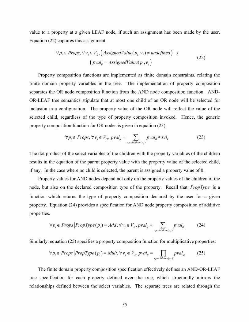
value to a property at a given LEAF node, if such an assignment has been made by the user.
Equation (22) captures this assignment.
( )
( ), , ( , )
( ,
i j L i j
ij i j
p Props v V AssignedValue p v undefined
pval AssignedValue p v
∀ ∈ ∀ ∈ ≠ →
= (22)
Property composition functions are implemented as finite domain constraints, relating the
finite domain property variables in the tree. The implementation of property composition
separates the OR node composition function from the AND node composition function. AND-
OR-LEAF tree semantics stipulate that at most one child of an OR node will be selected for
inclusion in a configuration. The property value of the OR node will reflect the value of the
selected child, regardless of the type of property composition invoked. Hence, the generic
property composition function for OR nodes is given in equation (23):
( )
, ,k j
i j O ij ikv children v
kp Props v V pval pval sel∈
∀ ∈ ∀ ∈ = ∗∑ (23)
The dot product of the select variables of the children with the property variables of the children
results in the equation of the parent property value with the property value of the selected child,
if any. In the case where no child is selected, the parent is assigned a property value of 0.
Property values for AND nodes depend not only on the property values of the children of the
node, but also on the declared composition type of the property. Recall that is a
function which returns the type of property composition declared by the user for a given
property. Equation (24) provides a specification for AND node property composition of additive
properties.
PropType
( )
( ) , ,k j
i i j A ij ikv children v
p Props PropType p Add v V pval pval∈
∀ ∈ = ∀ ∈ = ∑ (24)
Similarly, equation (25) specifies a property composition function for multiplicative properties.
( )
( ) , ,k j
i i j A ij ikv children v
p Props PropType p Mult v V pval pval∈
∀ ∈ = ∀ ∈ = ∏ (25)
The finite domain property composition specification effectively defines an AND-OR-LEAF
tree specification for each property defined over the tree, which structurally mirrors the
relationships defined between the select variables. The separate trees are related through the
55

select variable tree, since all OR-node property compositions depend on the values of the select
variables of its children.
Implementation of the Finite Domain Property Model
The property composition relations defined in the previous section define correctness criteria
for the enforcement of AND-OR-LEAF tree semantics with regards to property composition.
They do not, however, necessarily translate directly into an efficient finite domain model. As
with the implementation of the finite domain select variable relationships, the implementation of
the property composition finite domain model must take into consideration the concerns of
facilitating propagation during the search process.
The flexibility of Oz facilitates many different implementation approaches for the property
composition relationships. One such approach involves the literal implementation of the
mathematical relationships between property variables outlined above (see equations (23), (24),
and (25)). Another implementation path utilizes built-in symbolic Oz propagation routines to
model the semantic intention of the property composition relations. Both of these techniques are
employed in the Oz implementation of property composition relationships.
Figure 9 illustrates an Oz implementation of equation (24), additive property composition
for AND nodes. The procedure takes as parameters a list containing the property variables of the
children of the AND node in ChPropList, as well as the property variable for the AND node
itself in NodePropVar. It sets the property variable of the AND node equal to the sum of the
variables in the child property list, by invoking the FD.sum propagator provided by the Mozart
environment. This built-in propagator implements propagation in both directions, implying that
not only is the solver able to deduce information about NodePropVar based on the values and
domains of the variables in ChPropList, but the reverse is also the case: the solver can also
use domain information of the NodePropVar to deduce information on the property values of
the node’s children. Other DESERT-supported property composition types for AND nodes are
implemented in similar fashion. AND node property composition basically implements a literal
translation of the finite domain specification of the property composition function.
56

(1) proc {AndNodeAdditive ChPropList NodePropVar} (2) {FD.sum ChPropList ‘=:’ NodePropVar} (3) end
Figure 9. Oz implementation of the AND-node additive property composition relation defined in equation (24)
The implementation of property composition for OR nodes must be adapted from a literal
translation so as to facilitate propagation. Figure 10 provides a simple implementation of the
OR-node property composition relationship given in equation (23). The goal of the composition
relationship is to set the OR-node property variable equal to the value of the selected child. The
implementation below is passed four parameters, an ordered list containing the select variables of
the children of the OR node in ChSelList, the select variable for the OR node in NdSelVar,
an ordered list containing the property variables for the children of the OR node in
ChPropList, and the property variable for the OR node in NdPropVar. The fact that the two
lists are ordered is significant. The implementation assumes a correspondence between the child
select variable list and the child property variable list that is based on list order. The
implementation utilizes the FD.element constraint provided by Mozart to implement an
index-based list lookup operation. The list lookup facilitates propagation in both directions (i.e.
not only in the direction of the result of the look up, but also in the direction of the index
variable). The first FD.element statement attempts to look up from the list of select variables
a child variable whose value has the same value as that of the OR node select variable. The
index in the list of the matching child variable is assigned to the local variable SelChIndex (an
example of propagation in the “reverse” direction). The second FD.element statement uses
the SelChIndex value to look up the selected child’s property value, and to assign it to the OR
node property variable (an example of propagation in the “forward” direction).
(1) proc {BlkOrNdProp ChSelList (2) NdSelVar ChPropList NdPropVar} (3) SelChIndex = {FD.decl} (4) in (5) {FD.element SelChIndex ChSelList NdSelVar} (6) FD.element SelChIndex ChPropList NdPropVar} {(7) end
Figure 10. Blocking Oz implementation of the OR-node property composition relation defined in equation (23)
57

The OR-node property composition defined in Figure 10 does not facilitate efficient
propagation of property values across the tree. The outcome of the finite domain constraint
search process is a binding of values to the select variables that model selection or pruning in the
tree. However, the implementation above depends on grounded values of the select variables of
the children of the OR node in order to determine the OR-node property value. Hence, this
routine will block until the variables in ChSelList and ChPropList are all bound to single
values, relying completely on distribution to determine the values of the select variables for the
OR node children. Only after significant distribution can this procedure assign a value to the
property variable for the OR node.
The implementation in Figure 10 has been extended to facilitate propagation by including
redundant finite domain constraints that reflect variable interval information from the children to
the parent in the tree. During the search process, the actual values of all finite domain variables
are likely not bound to a particular value, but are known to be restricted to some finite domain.
While the implementation probably cannot, through propagation alone, determine the exact value
of the OR node property variable, in most cases it can further constrain the domain of the
variable. The extended implementation of OR node property composition posts constraints that
restrict the domain of the OR node property variable to reflect the minimum lower bound of all
its children, and the maximum upper bound of all its children. This extension is redundant with
respect to the implementation offered in Figure 10, in that when the selected child is found,
obviously the domain of the OR-node property variable will reflect the domain of the selected
child property variable (since they will be assigned to each other). However, the posting of the
redundant constraint facilitates the upward propagation of information much sooner in the search
process than would otherwise be allowed with the simple blocking implementation. Further, the
posting of the domain monitoring constraints constantly updates as propagators update the
domains of the child property variables, thus dynamically updating the OR node property
variable and facilitating further upward propagation.
A second redundant constraint is also added to the implementation given in Figure 10. It
may be the case that through the posting of constraints or through distribution that the domain of
the OR node property variable is modified. In that case, it may be possible to determine if a
child of the OR node has been NOT selected, by comparing the value of the property variable of
each child against that of the parent. Since the value of the OR node is set equal to the value of
58

the selected child, if a child’s domain is disjoint with the finite domain of the parent OR node, it
is safely concluded that the child cannot be selected. In such a case, the extended
implementation marks the child as being not selected. Note that the converse of this statement is
not true: It is not the case that if a child property variable is equal to the value of the parent, that
that child is automatically selected, since there may be multiple children with equivalent property
values. Figure 11 provides the extended Oz implementation, including the redundant constraints
discussed. Note that the two FD.element statements are enclosed in a thread block, due to
the fact that FD.element blocks when passed a list whose elements are not all bound to
values.
(1) proc { OrNodeProperty ChSelList (2) NdSelVar ChPropList NdPropVar} (3) SelChIndex = {FD.decl} (4) MaxChildVal = {ListMax ChPropList} (5) MinChildVal = {ListMin ChPropList} (6) in (7) thread (8) {FD.element SelChIndex ChSelList NdSelVar} (9) {FD.element SelChIndex ChPropList (10) NdPropVar} (11) end (12) (13) NdPropVar =<: MaxChildVal (14) NdPropVar >=: MinChildVal (15) (16) {List.forAllInd ChPropList (17) proc {$ Ind ChVal} (18) {FD.impl (ChVal \=: NdPropVar) (19) ({Nth ChSel Ind} =: 0) (20) 1} (21) end (22) } (23) end
Figure 11. Oz implementation of OR node property composition, including redundant constraints to facilitate propagation
The implementation of LEAF node property assignment is trivial, in that it is simply a
process of instantiating assignments of variables to values. The translation process which
59

instantiates the finite domain model inserts the appropriate assignment statements so as to
implement equation (22).
The finite domain model for representing DESERT properties and property composition was
outlined in the equations and figures above. Several issues were addressed that affect both
correctness as well as performance. In the case of OR node property composition, redundant
constraints were added to the specification to facilitate propagation early in the search process,
thus alleviating some of the dependence on distribution to achieve search results. To facilitate
performance of constraint satisfaction, the finite domain model implementation focuses on the
use of propagation to further the search process without affecting scalability.
Simple Property Example
Figure 12 extends the simple AND-OR-LEAF tree example from Figure 7 by adding an
additive property, called AP. For each LEAF node in the tree, the property value is bound to a
specific value, while the property values for nodes N1 and N4 are left unbound, to be determined
by the search process. The DESERT Property AP is designated an additive property, and is
associated with a property domain whose minimum bound is 0 and maximum bound is 32000.
Figure 12. Simple tree example, annotated with additive property AP
Figure 13 provides an Oz implementation of the finite domain model for the tree in Figure
12. In line (3), The Sel tuple is declared for the tree, just as in the example code in Figure 8.
Lines (4) and (5) give the declaration of variables NDMin and NDMax, which reflect the bounds
imposed by the property domain. Line (6) shows the declaration of the AP property tuple,
containing one variable per tree node, where each variable is initially constrained to the interval
60

defined by the property’s domain. Lines (8) and (9) establish the parent-child tree relationships
between the select variables for nodes N1 and N4, respectively. Lines (10)-(13) assign the AP
property values that are bound a-priori. Lines (14)-(15) establish for the OR node N4 the
property composition relationship between the property variable modeling the node (AP.4) and
the property variables modeling the node’s children (AP.5 and AP.6). Since the node is an OR
node, the OrNodeProperty procedure is invoked to establish these relationships. Line (15)
similarly establishes the property composition relationships between AND node N1 and its
children. Since AP is defined to be an additive property, and N1 is an AND node, the
AndNodeAdditive procedure is invoked. Since additive property composition at an AND
node does not depend on the select variables, it is passed only the property variables
corresponding to the children of the node (AP.2, AP.4 and AP.3), and the property variable
modeling the node property value (AP.1).
(1) proc {AppTree} (2) NumNodes = 6 (3) Sel = {FD.tuple sel NumNodes [0#1]} (4) NDMin = 0 (5) NDMax = 32000 (6) AP = {FD.tuple ap NumNodes [NDMin#NDMax]} (7) in (8) {AndNode [Sel.2 Sel.4 Sel.3] Sel.1} (9) {OrNode [Sel.5 Sel.6] Sel.4} (10) AP.2 =: 10 (11) AP.3 =: 20 (12) AP.5 = 7 (13) AP.6 = 5 (14) {OrNodeProperty [Sel.5 Sel.6] Sel.4 (15) [AP.5 AP.6] AP.4} (16) {AndNodeAdditive [AP.2 AP.4 AP.3] AP.1} (17) end
Figure 13. Oz implementation of the simple property example of Figure 12
Figure 14 shows the results of the invocation of the procedure defined in Figure 13. The
variables representing property AP have been constrained by the respective relationships. Note
that the property value at node N4 reflects the interval [5-7], indicating that it is yet
undetermined what the exact property value is. While the property variable for node N4 has not
61

been bound to particular value, its domain has been reduced to the interval [5-7], indicating that
the property value is 5, 6, or 7. The property value for node N1 is likewise bound to an interval,
as opposed to a particular value, pending an assignment to node N4’s property variable.
However, the interval at N1 has been reduced to reflect the interval at N4, indicating that the
property value at N1 will be 35, 36, or 37. The power of finite domain constraints is illustrated
in this example, in that although the problem specification did not directly result in a binding of a
value to N4’s property variable, it did constrain the value to a range. This constrained range
propagates upward in the tree, causing the range of the parent of N4 to be constrained as well. It
should also be noted that if the finite domain propagators utilized domain propagation instead of
interval propagation, the domain of N4’s property variable AP.4 would be restricted to the values
[5, 7]. However, domain propagation is considered expensive (evaluation of domain propagation
is highly enumerative and suffers from the same drawbacks as the over-reliance on distribution).
N1
N4
N3N2
N5 N6
AP=20
AP=5AP=7
AP=10
AP=[5-7]
AP=[35-37]
Figure 14. AND-OR-LEAF tree showing the results of finite domain propagation for the property AP
Summary of the Finite Domain Property Model
The finite domain model for DESERT properties and property composition mirrors the
relationships between the AND-OR-LEAF tree select variables. Finite domain variables are
used to represent property values at each node in the tree, and constraints implement tree
relationships between those variables. The implementation of the property model takes into
account several performance and scalability issues, in an attempt to establish a finite domain
model that relies highly on propagation for the determination of property values.
62

A Finite Domain Model for OCL Constraints
DESERT employs an extended subset of the Object Constraint Language (OCL) to allow the
modeler to specify restrictions on design space composition. These user-provided constraints
result in operations affecting the structure of the AND-OR-LEAF tree. This section outlines the
translation of the DESERT OCL constraint language into a finite domain constraint
specification.
DESERT implements only a subset of the Object Constraint Language, and extends that
subset with operations that facilitate the specification of design space pruning. Constraints are
assigned a particular application context, corresponding to a node in the AND-OR-LEAF tree.
Contexts in OCL are treated as objects, and context traversal is facilitated through functional
navigation. The application context for a constraint is returned by the OCL function self.
DESERT OCL supplies several functions to support tree navigation. For example, the parent
function may be invoked to access the context corresponding to the parent tree node of a context.
The children function may be invoked to access the children of a particular context (returned
as a list of contexts). The children function may also be used to access an individual child of
a context, by passing the name of the child as a parameter to the function. Constraints specify
relations between contexts, or between properties of contexts. DESERT registers all property
names as OCL function names, thereby allowing users to employ property names as functions in
the constraint specification in order to access context properties. DESERT offers the
implementedBy function to allow users to specify a binding of a choice in the design space
model. It can be employed to bind a particular child of an OR node to the OR node, thus
specifying the resolution to the choice modeled by the OR node. It may also be used to bind a
DESERT property at a particular context to a value in the property’s domain.
Figure 15 shows an example DESERT OCL constraint, relative to the example AND-OR-
LEAF tree from Figure 12. The context of the constraint is intended to be the node N4. The
constraint specifies a requirement that the context returned by self, in this case, node N4 is to be
“implemented by” the context named N5, corresponding to a child of N4. Since the context of
application refers to an OR node, the constraint specifies the requirement that node N5 be
selected as the outcome of the choice modeled by node N4.
63

constraint SelectConstraint() { self.implementedBy() = self.children(“N5”) }
Figure 15. Example DESERT OCL constraint, whose context is the node N4 from Figure 12
Logical, arithmetic and relational operations are supported in the specification of constraint
relations. Constraints typically specify an invariant relation that imposes some restrictions on the
design space model, and often, relational operators are used to specify quantitative bounds on
composed property values. Continuing the AP property example introduced in Figure 12,
suppose that a designer wishes to impose the constraint that requires that, regardless of how the
design space is composed, the composed property value at the root node be bounded by the value
35. A DESERT OCL constraint implementing the bound requirement is shown in Figure 16.
constraint APConstraint() { self.AP() <= 35 }
Figure 16. DESERT OCL constraint requiring the value of the context’s AP property not exceed 35
When the above constraint is associated with node N1 from Figure 12 as its context, it has a
pruning effect on the tree. Any configuration in the tree whose composed property value
exceeds 35 is pruned, or eliminated from consideration. The constraint solver is responsible for
implementing this pruning operation.
A Finite Domain Model for DESERT OCL Constraints
In order to apply DESERT OCL constraints to the finite domain constraint design space
model, the OCL constraints must be translated into finite domain constraints relating to the finite
domain representation of the AND-OR-LEAF tree. While the syntax of finite domain constraints
differs from that of DESERT OCL, the semantics of the two constraint languages are similar,
with respect to design space exploration and pruning. This section describes the semantic
translation of DESERT OCL constraints into a finite domain constraint representation.
Basic DESERT OCL constraints may be classified into two categories: those that relate two
constraint contexts, and those that relate one or more DESERT properties. Complex constraints
can be formed by composing constraints from these two categories using logical, relational and
64

arithmetic operators. Constraints that relate two contexts utilize the implementedBy function
to specify a binding between context objects. The only type of OCL collection that is currently
supported in DESERT OCL is a collection of contexts, as is returned by the children
function. List iteration is not supported (thus constraints cannot be posted against collections in
DESERT OCL).
The finite domain model for DESERT OCL constraints utilizes the finite domain variables
defined for the AND-OR-LEAF tree, as well as those defining the properties of the tree. A
DESERT property accessed by an OCL constraint at a context corresponds to the finite domain
property variable of the node that is represented by the context. Similarly, an OCL constraint
which relates two contexts is implemented as a relation between the Boolean select variables
modeled by each context. Navigation between contexts changes the point of access of tree
variables from one node to another. Since list iteration is not supported, all constraint navigation
functions can be resolved during the translation from OCL to the finite domain constraint
implementation.
OCL facilitates the specification of constraints that may or may not be satisfied. It does not
necessarily imply that a constraint must be satisfied. Hence, the translation algorithm separates
the specification of the constraint implementation from the specification of whether the
constraint must be satisfied or not. Reification of the constraint implementation statements is
employed by the translator in order to implement this separation. Requirements on whether a
constraint should be satisfied can themselves be formulated as constraints on the reified
constraint variables.
Figure 17 shows a finite domain implementation of the DESERT OCL constraint from
Figure 15. The implementedBy function is implemented as an equivalence constraint
between the select variables corresponding to the related contexts. The application context for
the constraint is node N4, whose select variable is denoted Sel.4 (the member of the Sel tuple
whose index is 4, corresponding to the ID of node N4). On the right hand side of the operation,
constraint navigation is used to navigate to the context corresponding to node N5. The select
variable corresponding to node N5 is denoted Sel.5. Line (1) below specifies that the select
variable of node N4 is required to be the same as that of node N5, specifying that if either is
determined to be selected, then both must be selected. This equation constraint is reified into the
temporary Boolean variable TmpBool.1. Note that the constraint does not necessarily imply
65

that the select variable of node N5 takes on the value 1, since it is unknown at translation time
whether the parent OR node itself has been selected.
The implementedBy function when applied at an OR node context not only implies the
binding of one child to the parent, but also implies that all remaining children cannot be selected.
Line (2) implements the reified zeroing of Sel.6, corresponding to the only other child of N4.
Line (3) reifies the conjunction of the reified results of the translated statements into
TmpBool.3. Since the constraint in Figure 15 is specified as requirement of the design space
composition, the translated constraint statements must be satisfied. Hence, line (4) posts the
constraint on TmpBool.3, requiring that it, and equivalently all the above reified variables, take
the value 1.
(1) TmpBool.1 =: (Sel.4 =: Sel.5) (2) TmpBool.2 =: (Sel.6 =: 0) (3) TmpBool.3 =: {FD.conj TmpBool.1 TmpBool.2} (4) TmpBool.3 =: 1
Figure 17. Oz implementation of the DESERT OCL constraint from Figure 15
A DESERT OCL constraint that refers to a DESERT property accesses a finite domain
variable that models the property value at the context of the OCL constraint. Figure 18 shows
the Oz implementation of the OCL constraint depicted in Figure 16. Line (1) contains a
reification of the constraint implementation, with line (2) implementing the requirement that the
constraint be satisfied. The AP function invoked on the context of constraint application returns
the finite domain variable modeling the AP property at the node corresponding to that context, or
in this case, node N1. The AP property variable for node N1 is AP.1, the variable in the AP
property tuple which corresponds to N1’s ID. Thus the OCL constraint imposes the finite
domain constraint that stipulates that the finite domain variable AP.1 must take on a value
which is less than or equal to 35.
(1) TmpBool.4 =: (AP.1 <=: 35) (2) TmpBool.4 =: 1
Figure 18. Oz implementation of the DESERT OCL constraint from Figure 16
66

DESERT OCL Constraints and Finite Domain Propagation
DESERT OCL constraints facilitate the specification of restrictions on design space
composition. Constraints either specify bindings between select variables, or restrict domains of
property variables. The addition of a constraint to the finite domain constraint store adds
information to the store, potentially invoking propagation. Property composition functions
specify the “upward” propagation of information, by defining the property value of a node in
terms of the values of its children. In contrast, the specification of an OCL constraint on an
interior node of the AND-OR-LEAF tree facilitates the “downward” propagation of information.
The constraint propagators discussed above have been implemented so as to facilitate
propagation in both directions across the tree. A goal of downward propagation is to determine
which variables, if any, cannot be selected due to the imposition of OCL constraints. Interval
propagation of composed property values can result in the binding of values to select variables
through the definition of property composition at an OR node. The “bi-directionality” of
propagation offered by the tree relation implementation is a key performance attribute of the
finite domain design space implementation.
Summary of Finite Domain Model for OCL Constraints
DESERT OCL constraints are translated into finite domain constraints to facilitate the
specification of user-defined tree pruning operations and their application to the finite domain
AND-OR-LEAF tree representation. Operations on context objects are implemented as relations
between select variables. OCL constraint operations involving DESERT properties are
translated into operations involving the finite domain variables that model the DESERT
properties. The implementation of finite domain property composition and the implementation
of select variable tree relations both facilitate the downward propagation of information specified
by the OCL constraint at its context of invocation.
Finite Domain Distribution
The finite domain model of the DESERT AND-OR-LEAF tree, properties and OCL
constraints has been developed so as to facilitate a high degree of propagation during the search
process. However, as noted in Chapter II, in general, propagation alone is not sufficient to
implement a complete constraint solver. While Mozart provides basic distribution algorithms
67

that implement a set of heuristics that have been shown to be generally effective, a customized,
application-specific distribution algorithm can utilize knowledge of the problem structure to
better tailor distribution to fit the propagation model. This section outlines a customized
distribution algorithm that implements several heuristics to facilitate a rapid resolution to the
finite domain design space search problem.
An examination of propagation patterns from the finite domain design space model reveals
several strategies for the implementation of distribution heuristics. As discussed above, the
implementation of tree relationships between select variables, as well as those between property
variables, facilitates both “upward” and “downward” tree propagation. The addition of
information about a variable can have far-reaching effects in the tree due to propagation. The
propagation model for an AND node equates the select variables of the children of the node to
their parent, facilitating propagation in either direction. Downward propagation halts at an OR
node, since search must determine the outcome of the choice modeled at an OR node. However,
if a child of an OR node is determined to be selected, upward propagation is facilitated. Due to
this fact, if a select variable chosen at random for distribution, binding the variable as selected
potentially results in greater propagation than marking it as not selected. Distribution on a select
variable results in two contradictory spaces, one where the select variable is bound to the value 1,
and one where it is bound to 0. The distribution algorithm employs the “SelectFirst” heuristic
when determining the order in which to search the resulting cloned spaces. Algorithm 1
specifies the distribution algorithm applied to select variables. The algorithm is passed in
SelVarList a list of select variables which have not yet been bound to values. The
CloneSpace function clones the current computational space, and creates a thread wherein the
evaluation of the cloned space proceeds. The function returns a true value in the caller thread,
and false in the newly created thread. In the former case, line (4) sets the select variable to 1,
while in the latter, line (6) sets the variable to the value 0.
68

(1) DistributeSel(SelVarList) (2) let s be the head of SelVarList (3) if CloneSpace() { (4) post(“s = 1”) (5) else (6) post(“s = 0”) (7) } (8) end
Algorithm 1. Distribution algorithm for distributing select variables
The distribution algorithm must also consider property variables as candidates for
distribution. The goal of the finite domain search is to bind all select variables to values, to
determine a valid configuration that meets the modeled constraints. However, it is often the case
that the DESERT OCL constraints involve operations on DESERT properties. The propagation
model for property composition outlined above facilitates upward and downward propagation of
property values. Property composition for an OR node depends directly on the select variables
of the node and the children of the node. Hence, property composition can affect tree node
selection. Due to the size of a select variable domain, distribution on a select variable can
produce only two constraints. However, the domain of a property variable is typically much
larger than that of a select variable, requiring the application of a distribution heuristic.
The distribution algorithm, when selecting between property variables, must determine
which variable to distribute on, as well as how to formulate the constraints to insert into the
cloned spaces. The algorithm appeals to the first-fail heuristic to address the issue of variable
selection. The list of unbound property variables is sorted according to domain size, whereon a
variable whose domain size is minimal is selected for distribution. The algorithm then employs a
domain-splitting heuristic to formulate two contradictory constraints. Let pv be the chosen
property variable. Let be a function which returns the finite domain of a finite
domain variable. Let be the midpoint
of the domain of the selected property variable. Then, for distribution on
FDDomain
( )( ( )) ( ( ))m max FDDomain pv min FDDomain pv⎡ ⎤= −⎢ ⎥/ 2
pv , the distribution
algorithm generates the following two contradictory constraints: pv m< and pv m≥ . Since it
is not clear that either cloned space will be more likely than the other to more effectively induce
propagation, neither space is favored during the search. Algorithm 2 gives the implementation of
the distribution of property variables. It is passed a list of as-yet unbound property variables.
69

(1) DistributeProperty(PVList) (2) Let pv in PVList be chosen such that (3) FDDomain(pv) is minimal (4) if CloneSpace() { (5) post(“pv < m”) (6) else (7) Post(“pv >= m”) (8) } (9) end
Algorithm 2. Distribution algorithm for distributing on property variables
Prior to the application of the above algorithms, the distributor filters the set of variables
available for distribution. Algorithm 3 gives the implementation of the variable filtering
algorithm. The algorithm is passed a list of records, where each record contains the select
variable and the set of property variables corresponding to a tree node. During the finite domain
search process, it may be the case that a select variable for a node has been bound to a value,
while one or more of the node’s property variables remain unbound. Conversely, it may also be
the case that one or more of the property variables are bound to values, while the select variable
remains unbound. It represents wasted effort to distribute on an unbound property variable
whose node has been marked as unselected, since that variable’s property value does not affect
the property values higher in the tree. Hence, the FilterTreeList algorithm filters out not
only those variables which have been bound to values, but also those property variables whose
nodes have been marked as unselected. Filtration separates the node variables into two lists, one
containing unbound select variables, and the other containing unbound property variables.
70
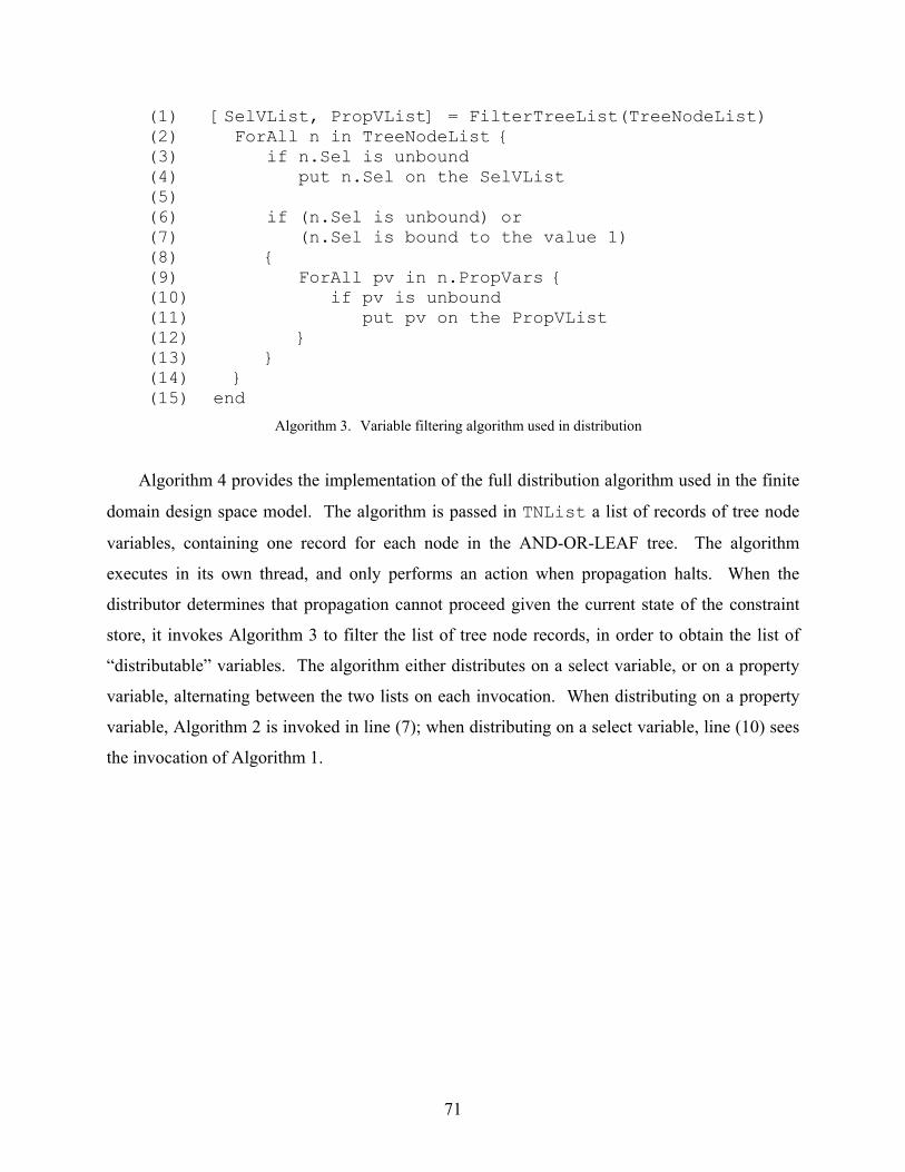
(1) [SelVList, PropVList] = FilterTreeList(TreeNodeList) (2) ForAll n in TreeNodeList { (3) if n.Sel is unbound (4) put n.Sel on the SelVList (5) (6) if (n.Sel is unbound) or (7) (n.Sel is bound to the value 1) (8) { (9) ForAll pv in n.PropVars { (10) if pv is unbound (11) put pv on the PropVList (12) } (13) } (14) } (15) end
Algorithm 3. Variable filtering algorithm used in distribution
Algorithm 4 provides the implementation of the full distribution algorithm used in the finite
domain design space model. The algorithm is passed in TNList a list of records of tree node
variables, containing one record for each node in the AND-OR-LEAF tree. The algorithm
executes in its own thread, and only performs an action when propagation halts. When the
distributor determines that propagation cannot proceed given the current state of the constraint
store, it invokes Algorithm 3 to filter the list of tree node records, in order to obtain the list of
“distributable” variables. The algorithm either distributes on a select variable, or on a property
variable, alternating between the two lists on each invocation. When distributing on a property
variable, Algorithm 2 is invoked in line (7); when distributing on a select variable, line (10) sees
the invocation of Algorithm 1.
71

(1) DistributeVars(TNList) (2) bool isPropTurn = false (3) forever { (4) wait for current computation space (5) to complete all propagation (6) [SelVList, PropVList] = FilterTreeList(TNList) (7) if isPropTurn { (8) DistributeProperty(PropVList) (9) isPropTurn = false (10) else (11) DistributeSel(SelVList) (12) isPropTurn = true (13) } (14) } (15) end
Algorithm 4. Distribution algorithm implementing finite domain design space search
Constraint Utilization and Finite Domain Search
The third component of a complete finite domain solver, after propagation and distribution,
is search. Mozart offers three general options for implementing search: search for one result,
search for all results, and search for the best result. Best-case search employs a branch-and-
bound algorithm together with a user-provided solution evaluation function in order to maximize
a solution quality metric. The finite domain model for DESERT utilizes the built-in search
algorithms in different contexts, depending on the use-case of the finite domain search.
Single-Solution and All-Solution Search
The finite domain model outlined in this chapter can be used to quickly find a single
solution to the design space problem. A solution to the search problem represents a single
configuration in the design space, which satisfies all user-provided constraints. Simple depth-
first search through the distribution tree results in a single solution to the finite domain design
space model with a minimal number of distribution steps.
All-solution search can be employed to calculate all valid solutions to the finite domain
model. All-solution search simply continues the one-solution search depth-first search
algorithm. When a solution to the problem is encountered, it is added to a solution list. All-
solution search exhaustively explores the full design space. The challenge with all-solution
search is that the number of solutions in a design space may be very large. Distribution
72

implements a partial enumeration of the space, where, at each distribution step, each of the
cloned spaces potentially contains several solutions. Distribution must be performed in order to
obtain the list of solutions. The enumeration of an exponential number of solutions causes the
finite domain search process to terminate prematurely due to exponential growth in memory
requirements.
In contrast, the symbolic constraint representation approach employed in DESERT does not
depend on partially enumerative techniques in order to apply constraints. Constraints are applied
to the symbolic representation of the space, resulting in a pruned OBDD representation. This
pruned representation holds all valid configurations of the space. After pruning terminates, the
BDD library can be used to determine if the pruned space contains a large number of
configurations, in which case DESERT warns the user to apply more constraints. Since the
process of pruning the finite domain representation of the space involves partial enumeration,
there is no equivalent operation to determine, after all constraints have been applied, how many
configurations result. However, the finite domain search process can be terminated prematurely,
on detection of an exponential growth in the number of solutions.
Constraint Utilization and Best-Solution Search
The disadvantage of space enumeration brought on by all-solutions search has motivated the
implementation of a best-case search. The finite domain model for design space exploration
extends DESERT by allowing the conversion of under- and over-constrained design spaces into
near-critically constrained spaces, through the concept of constraint utilization. DESERT OCL
constraints are grouped by the modeler into sets, where each set is assigned a utilization number.
The utilization number applies to each member of the set, and indicates the relative importance
of producing design compositions where the constraints contained in the set are satisfied. In the
case where the modeler wishes to require that a constraint be applied to the space irrespective of
the utilization outcome, the constraint is assigned to a constraint set whose utilization index is -1.
Best-case search in Mozart attempts to maximize total constraint utilization, by searching for
solutions whose total constraint utilization is maximal. Total constraint utilization is simply the
sum of all utilization numbers of all constraints that are satisfied for a given solution. Recall the
formal definition of a configuration Cfg given in equation (16). Let
( )Configs P V sol Configs⊆ ∀ ∈ , is a configuration. Let be a function which sol :cutil CS →
73

returns the user-provided constraint utilization number for a constraint. Let
be a function which calculates the utilization of a configuration. Then equation (26) defines the
utilization function Ut .
:Util Configs →
il
, ( ) (c CS sol c
sol Configs Util sol cutil c∈ →
∀ ∈ = )∑ (26)
The Oz implementation of constraint utilization is accomplished through constraint
reification. All finite domain implementations of DESERT OCL constraints must be reified in
order to facilitate the determination of which constraints have been satisfied and which have not.
In the case of constraint utilization calculation, it is assumed that some constraints will be
satisfied, while others will not. The search process determines which constraints are indeed
satisfied and thereby contribute to the constraint utilization function. The constraint utilization
calculation can be converted into a simple multiply-add operation over the set of reified
constraint variables, as shown in equation (27). The ( solc TRU== )E expression indicates the
reification of the evaluation of constraint c over solution into a 0/1 variable. Where the
constraint is satisfied for a solution, the reified variable takes on the value 1. Where the
constraint is not satisfied, the variable takes on the value 0 and therefore does not contribute to
the total utilization sum. The use of reified constraint variables simplifies the implementation of
the utilization calculation.
sol
( ) ( ) ( )solc CS
Util sol cutil c c TRUE∈
= ∗ ==∑ (27)
Constraint reification facilitates the determination of constraint utilization. Constraint
utilization facilitates the conversion of an over-constrained design space into a near-critically
constrained design space. The modeler simply assigns to each constraint a utilization number,
and the search implements a best-case search to maximize utilization. However, as a
consequence of the assignment, not all constraints specified in the over-constrained space will be
satisfied. An over-constrained design space has no solution which satisfies all constraints. A
best-case search solution using constraint utilization approximates the best solution possible for
the over-constrained solution. Constraint utilization calculations can also be used to map an
under-constrained space to an over-constrained space, by supplying more constraints.
74
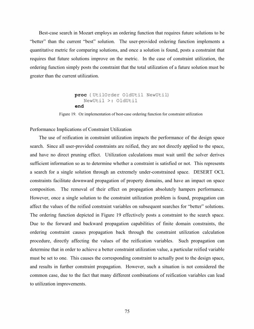
Best-case search in Mozart employs an ordering function that requires future solutions to be
“better” than the current “best” solution. The user-provided ordering function implements a
quantitative metric for comparing solutions, and once a solution is found, posts a constraint that
requires that future solutions improve on the metric. In the case of constraint utilization, the
ordering function simply posts the constraint that the total utilization of a future solution must be
greater than the current utilization.
proc {UtilOrder OldUtil NewUtil} NewUtil >: OldUtil end
Figure 19. Oz implementation of best-case ordering function for constraint utilization
Performance Implications of Constraint Utilization
The use of reification in constraint utilization impacts the performance of the design space
search. Since all user-provided constraints are reified, they are not directly applied to the space,
and have no direct pruning effect. Utilization calculations must wait until the solver derives
sufficient information so as to determine whether a constraint is satisfied or not. This represents
a search for a single solution through an extremely under-constrained space. DESERT OCL
constraints facilitate downward propagation of property domains, and have an impact on space
composition. The removal of their effect on propagation absolutely hampers performance.
However, once a single solution to the constraint utilization problem is found, propagation can
affect the values of the reified constraint variables on subsequent searches for “better” solutions.
The ordering function depicted in Figure 19 effectively posts a constraint to the search space.
Due to the forward and backward propagation capabilities of finite domain constraints, the
ordering constraint causes propagation back through the constraint utilization calculation
procedure, directly affecting the values of the reification variables. Such propagation can
determine that in order to achieve a better constraint utilization value, a particular reified variable
must be set to one. This causes the corresponding constraint to actually post to the design space,
and results in further constraint propagation. However, such a situation is not considered the
common case, due to the fact that many different combinations of reification variables can lead
to utilization improvements.
75

A second effort attempts to partially rectify the performance implications of the use of
constraint utilization and reification. The reification variables can be added to the distribution
list, allowing the distribution process to assign a value to the reified variable, thereby causing the
constraint to be posted in one of the distributed subspaces, resulting in what propagation effects
the constraint brings about. Such distribution can also short-circuit the constraint utilization
calculation by “guessing” early on that a constraint is satisfied and calculating the resulting
utilization value. The remaining constraint relations ensure that such a guess is correct (if not the
search is halted at this node).
Summary of Constraint Utilization techniques
The use of constraint reification to facilitate utilization computations allows a unique
approach to design space exploration. Best-case solutions to over-constrained spaces can be
approached, by modeling the relative importance of whether a given constraint actually is
satisfied in a search outcome. The use of constraint reification to implement utilization hampers
performance, but due to the strength of the propagation model, the performance degradation does
not render the approach unusable.
Summary of the Finite Domain Constraint Model for DESERT
A finite domain constraint model for representing and exploring design spaces has been
developed. The model implements the semantics of the DESERT AND-OR-LEAF tree through
finite domain constraint relations over variables that model different aspects of the tree. Boolean
finite domain variables model inclusion in or exclusion from a configuration. DESERT
properties are modeled as finite domain variables, and property composition is implemented as a
set of relations between property variables. DESERT OCL constraints are mapped onto the
finite domain representation as relations involving the variables modeling different aspects of the
AND-OR-LEAF tree. The model offers a customized distribution algorithm that tailors
distribution decisions to the structure of the finite domain model. Search is implemented using
the built-in Mozart search facilities, and all three classes of search are supported. Since
distribution and search naturally enumerates the design space, a best-case search approach has
been implemented to convert over-constrained and under-constrained design spaces into near-
76

critically constrained spaces. The approach attempts to maximize constraint utilization for the
set of constraints assigned by the modeler.
Many performance considerations have been addressed in the development of the finite
domain model. The AND-OR-LEAF tree relationships have been crafted so as to facilitate the
propagation of values and intervals, where appropriate up and down the tree. Property
composition routines facilitate the imposition of constraints from above, and values from below,
and can propagate information in either direction to facilitate the search. The distribution
algorithm implements several problem-specific heuristics when selecting variables for
distribution, and also when devising constraints on those variables. The goal of the distribution
algorithm is to facilitate as much propagation as possible, in as few distribution steps as possible.
The constraint utilization techniques outlined above degrade performance, due to the diminished
role of a constraint through reification. However, the finite domain model attempts to partially
rectify this degradation by facilitating propagation across the utilization calculations through to
the reification variables, and by distributing on reified constraint variables.
77

CHAPTER IV
THE PROPERTY COMPOSITION LANGUAGE
DESERT facilitates the modeling of property composition through a limited suite of
property composition functions. These functions represent classes of operations that define a
tree node’s property value in terms of some mathematical operation on the property values of the
node’s children. This chapter discusses the modeling limitations on property composition
specification imposed by the current DESERT approach, both in computational tractability and
in expressiveness. To address these limitations, a language called PCL (Property Composition
Language) has been developed to facilitate expressive modeling of complex property
composition functions. Tools have been developed to translate PCL statements into a finite
domain constraint representation that leverages the finite domain model of the AND-OR-LEAF
tree. This chapter outlines the design of PCL, as well as the finite domain representation and
translation of the language.
Limitations in Modeling Property Composition
The expressiveness of the DESERT property composition functions is overly restrictive. A
property composition function is an implementation of a mathematical function that models the
calculation of a property value at a node in terms of the property values of the children of the
node. In general, property composition is difficult to model, often requiring complex
mathematical relationships. For example, consider a latency property of a multi-processor,
signal processing application. The calculation of the composed latency property involves a
longest path analysis across the application graph, and must take into account computational
resource sharing and scheduling, and communication bandwidth, delays and resource sharing.
Such complex calculations cannot be modeled as a simple, one-dimensional mathematical
operation, such as those offered by DESERT. While DESERT offers the capability of
developing “custom” property composition routines as a plug-in to the solver framework, the
development of such routines is cumbersome and requires developer knowledge of the internal
DESERT data structures.
78

Neema reports on the scalability issues of the OBDD approach that are encountered when
performing complex mathematical operations in DESERT [79]. The OBDD representation of
the design space actually utilizes multi-terminal binary decision diagrams (MT-BDDs) to
facilitate the representation of data in mathematical operations. The MT-BDD representation
utilizes integers as the terminal nodes in the data structure, as opposed to the 0 and 1 terminal
nodes in the OBDD structure. An MT-BDD structure achieves a high degree of compaction in
representation size when there is a significant re-use of terminal values. When there is not a high
degree of reuse of terminal nodes, the MT-BDD representation can become exponential. In the
case where the DESERT domain of the property contains a wide range of numbers, it is highly
likely that such an MT-BDD explosion will occur. The observed behavior of the DESERT
BDD-based pruning indicates that for design spaces requiring the representation and evaluation
of mathematical operations, the BDD quickly becomes exponential in memory size as the
problem size scales up. Pruning of highly orthogonal design spaces is also prohibitively
expensive in the presence of mathematical operations. The BDD representation of the design
space does scale well as a representational mechanism (Neema reports the ability to represent
spaces of up to different configurations), and as a coarse-grained pruning approach, so long
as the pruning operations do not involve mathematics that cause the BDD representation to
explode.
18010
The lack of expressiveness for modeling complex property composition relationships, as
well as the lack of scalability for implementing simple property composition relationships
implies a serious flaw in the DESERT toolset. The work presented in this chapter rectifies this
flaw, through the development of a property composition language that is sufficiently expressive
so as to facilitate the modeling of complex relationships. The implementation of the language
must scale to large problem sizes without incurring an exponential explosion in memory or
execution time.
The Property Composition Language
The Property Composition Language is a simple scripting language that supports the
specification of both linear and non-linear mathematical operations involving multiple properties
and multiple types of properties. Tree navigation is fully supported, in similar fashion to
DESERT OCL.
79

PCL Variables, Operations, Expressions and Statements
PCL is a typed programming language that provides a simple syntax for modeling property
composition operations. There are only two data types supported in PCL: var and list. var
represents a variable, a placeholder for a single value, that can be assigned to and read from. In
PCL, all variables (either var or list) are single-assignment, in that once a variable has been
assigned, it cannot be re-assigned. A PCL list represents a list of variables. Lists of lists are
not supported, and the length of a list must be well-defined when a PCL specification is
interpreted. Properties can be accessed as PCL vars through provided property access
operations. Iteration through lists is performed using customizable list iteration operations that
are provided with PCL.
PCL supports mathematical operations between variables. A full host of operations are
supported, including arithmetic, logical and relational operations. Linear arithmetic operations,
such as addition, subtraction and multiplication are supported, as are non-linear operations, such
as integer division, modulo arithmetic, and integer exponentiation (a variable raised to an integer
power). Supported logical operations include conjunction, disjunction, implication, equivalence,
and logical negation. Relational operations define variable comparisons, utilizing the following
operations: greater-than, less-than, equal-to, not-equal-to, greater-than-or-equal-to, less-than-or-
equal-to. Other comparison operations include min and max, which return the minimum and
maximum, respectively, of two variables.
Operations involving one or more variables and one or more operators are collected into
PCL expressions. PCL operations are specified through operators (the syntax of the operators is
provided in Appendix A, which contains the input specification for lexical analysis of PCL, and
Appendix B, which contains the context free grammar of PCL). There are two classes of
operators supported in PCL: binary operators and unary operators. Unary operations include
logical negation and arithmetic negation. The remaining operators discussed above are binary
operators. An operator, together with its argument(s) defines an expression. Operators may take
expressions as arguments. An expression models a value, the result of the evaluation of the
expression on its arguments. By virtue of the recursive nature of the expression definition, an
expression can be large and complex, involving multiple variables and multiple operations. PCL
supports the use of parentheses to disambiguate operation association, and to form a single
80

expression from a set of expressions. The formulation of PCL expressions is similar in concept
to the formulation of expressions in C or other high-level programming languages.
PCL allows variable assignment. All variables are single-assignment variables, in that a
variable may be assigned to only once. Variables that are never assigned to should not be read
from, and the PCL parsing and evaluation tools output a warning when such a circumstance is
encountered. Variables are defined (or assigned to) using the assignment operator. A valid
assignment involves the assignment to a variable of any valid PCL expression that is type-
equivalent to the variable. Type equivalence implies that only expressions that evaluate to
simple variables may be assigned to simple variables, while only expression that evaluate to list
variables may be assigned to list variables. Type equivalence on assignment is verified during
PCL evaluation.
Variable assignment is a type of PCL statement. In contrast to an expression, a statement
does not represent a value. Thus, assignments may not be “chained” together, as in C (i.e.
a=b=c=d is not a legal PCL statement). PCL supports other types of statements as well,
including declaration statements, control statements, and call statements. A declaration
statement contains a variable declaration, possibly including an initialization assignment to some
expression. All PCL variables must be declared prior to use. A control statement represents an
if-then-else decision statement. Although the language syntax supports if-then-else statements,
the PCL evaluation does not currently support decisions at the implementation level. Call
statements represent invocations of PCL functions, which are discussed below.
Modularity in PCL: Properties and Functions
All statements in PCL are defined within a function. A function is a collection of PCL
statements. A function has a set of formal input parameters, and can return a variable. A special
type of function is defined as a property. A property function defines a DESERT
property, and represents a PCL entry point. The variable returned by a property function is
associated with a DESERT property, allowing the operations defined in and invoked by the
function to define the property value. Other than this point, a property definition is no
different from that of any other PCL function. PCL functions that are not defined with the
property keyword are identified with the keyword function. The use of functions in PCL
facilitates a modular approach to the specification of property composition.
81

A function contains a set of statements. All statements in a function form a block, which
defines a scope for the definition of variables. All scopes are local, in the sense that a variable is
only visible within the scope where it is declared. All variables must be defined within a scope,
and global variables are not supported. If a new block is entered (in the case where a function is
invoked), only variables defined within the new scope are available for access. All functions, on
the other hand, are defined in a single global namespace. Local function definitions are not
supported. The formal parameters of a function are treated as initialized variable declarations,
and are visible within the scope defined by the function’s block. A return statement may be
placed anywhere within the block defined by a function, causing the evaluation of the function to
return control (and any associated return expression) to the caller.
Function invocations are allowed in two different locations in PCL. A function that returns
a variable can be invoked as part of an expression. Any function can be invoked as a statement,
where the expression returned by the function, if any, is ignored. Note that due to the scoping
rules imposed by PCL, except under special circumstances, such function invocations typically
do not accomplish anything.
Tree Navigation
OCL statements apply at a particular context. A PCL property specification, likewise,
applies at a context, corresponding to a node in the AND-OR-LEAF tree. The specification
defines a DESERT property corresponding to the context of invocation. However, unlike OCL
statements, PCL specifications are evaluated over several contexts, owning to the fact that
composed properties are defined over all nodes in the tree. PCL abstracts the particulars of
which node the statements are applied to into the concept of a context, and tree navigation is
facilitated through functional operations relative to the invocation context. Such tree navigation
is pattered after the navigation capabilities of DESERT OCL. Built-in PCL functions allow
access to different contexts. The parent function returns the parent of the current context. The
children function returns a list of context objects, representing the children of the current
context. A specific child may be accessed by passing the child’s name as a string literal to the
children function. Calls to functions that access or change contexts can be chained together
using the dot operator syntax, passing the result context of a function call as the invocation
context of the next function call. The self function returns the original invocation context of
82

the PCL specification. The PCL syntax for tree navigation differs slightly from the OCL
navigation syntax, in that PCL employs function invocation syntax instead of the simple dot-
object syntax used in OCL. For example, a statement to access all the children of the parent of
the current context in OCL appears as: self.parent.children, where as in PCL, the
statement appears as self().parent().children().
Tree navigation is typically used to navigate to a particular context, which is then used to
access a property variable for that context. Property access is facilitated through the prop
function, provided in PCL. The name of the property being accessed is passed as a string literal.
The function sel returns a Boolean variable whose value indicates whether an invocation
context has been marked for inclusion or exclusion from the set of configurations in the design
space. These property access functions are invoked at the end of a tree navigation statement,
with the same dot operator syntax. Both of these property access functions can be invoked on a
simple context, as well as on a list of contexts. When invoked on a list of contexts, the function
implicitly loops through the list and applies the simple function on each list member and collects
the results into an output variable list. For example, self().property(“area”) returns a
variable representing the area DESERT property belonging to the invocation context, while
self().children().property(“area”) returns a list of variables corresponding to
the area property variables belonging to the children of the invocation context.
List Iteration Functions
General user-defined iteration is not supported in PCL. However, limited support is
available for iteration through a list of variables. Such iteration is effected through “built-in” list
iteration functions. These functions visit each member of the list, from head to tail, and invoke a
user-specified function on each list member. The user passes the name of the node-visitation
function as a parameter to the iteration function. The PCL evaluator algorithm handles the
mechanics of passing the list node to the node visitor. Only two list iteration functions are
supported, which differ based on what is done with the results of a node visitation. The ForAll
list iteration function accepts two parameters, the list to iterate over, and the name of the visitor
function to invoke when visiting a node. The visitor function must accept a single variable: the
list member, and must return a simple expression. ForAll collects each expression returned by
the node visitor function into a list and, after finishing the list iteration, returns the list of
83

returned expressions. The ForAllAcc returns a single expression that represents the
accumulated result of visitation of each node. As with ForAll, ForAllAcc is passed a user-
specified node visitor function. However, in contrast to the ForAll node visitor function, the
ForAllAcc node visitor is passed not only the list member, but also an expression representing
the accumulated results of the previous node visitations. The node visitor is responsible for
visiting the node and accumulating the results of the visit with the previously accumulated visit
results. This new accumulation expression is returned to the list iteration function, and passed to
the node visitor on invocation for the next list member. On exhaustion of the list, the list
iteration function returns the accumulation expression to the caller. ForAllAcc takes three
parameters, the list to iterate over, the name of the visitor function, and an initial accumulator
value.
Simple PCL Example: Area Property
Figure 20 provides a simple example of a PCL property composition specification. The
property being modeled is a simple additive property called area. Such a specification could be
employed when modeling the composition of FPGA configurations. The area property
composition allows a user to specify a constraint on the total area of a composition, requiring
that a composition fit in the available gate area. While gate area is not necessarily a simple
additive property, a coarse-grained model suffices to illustrate the PCL implementation. Line (1)
defines the helper function SumVar, which is later used as a list node visitor function. Line(5)
defines the entry point to the area property calculation, with a property declaration called
areaProperty. Line (6) obtains a list of area property variables, corresponding to the
children of the context of invocation. The list is stored in the list variable chAreaProps. Line
(7) illustrates the invocation of the ForAllAcc list iteration function. The function is passed
the chAreaProps list as the list to iterate on, followed by “SumVar,” the name of the
function to invoke while visiting each member of the list. The third parameter is the integer
literal 0, representing an initial accumulation value of 0. Line (1) begins the definition of the
visitor function SumVar, which is invoked by the ForAllAcc function. This function takes
two parameters, v1, representing the visited list member, and v2, representing the accumulated
results of the previous list member visits. Line (2) sees the return of the addition of v1 to v2. In
84

the context of list accumulation, this simply takes the current list member, adds it to the
accumulator and returns the summed result. The ForAllAcc function returns the results of
accumulation across all list members, and line (7) sees that value stored into a newly declared
variable named ret. In line (8), the variable ret is returned, effectively assigning the results of
accumulation to the area property of the invocation context.
(1) function var = SumVar(var v1, var v2) { (2) return (v1 + v2); (3) } (4) (5) property areaProperty( ) { (6) list chAreaProps= self().children().prop(“area”); (7) var ret = ForAllAcc(chAreaProps, “SumVar”, 0); (8) return (ret); (9) }
Figure 20. Example PCL function modeling an additive property called area
PCL Interpretation
PCL is designed to facilitate dynamic interpretation. Specifically, a design goal of PCL was
to avoid the need of invoking a separate language compiler to generate an executable
specification. Otherwise, the design space exploration tools would need to be rebuilt after any
change to a user-defined PCL specification. Instead, the PCL interpreter has been designed to
dynamically compile and interpret a PCL specification. The execution semantics of PCL is built
on the finite domain design space model, discussed in Chapter III. The PCL interpreter is tasked
with the translation of a PCL specification into an equivalent finite domain specification that can
form part of the finite domain design space search.
Expression Trees
The mapping of PCL statements into finite domain constraints centers on the development
of a finite domain expression tree. An expression tree models a complex chain of operations that
evaluates to a value. The PCL interpreter translates a PCL specification into a set of PCL
expression trees, and then maps the set onto a set of finite domain expression trees. Finite
domain expression trees have execution semantics assigned by the finite domain constraint
solver, and therefore can be evaluated as the finite domain design space model is pruned.
85

However, the translation process begins with the evaluation of a PCL specification, which results
in the construction of a PCL expression tree.
Formally, a PCL expression tree is a tree:
, ,T V E VT= (28)
where,
is a set of vertices; V
is a set of directed edges; and E VxV⊆
is a function mapping a vertex to a vertex type. : { , ,VT V BinOp UnOp Leaf→ }
An expression tree models a set of PCL operations. Vertices in the tree model operations
between sub-trees. Leaf nodes in the tree model variables or data, items which are not refined
further by the PCL specification. The vertex type denotes the type of operation modeled by the
node: BinOp indicates a binary operation; UnOp indicates a unary operation; and
indicates the vertex models data as opposed to an operation, and represents a leaf node in the
tree. Edges in the tree connect operations to operands.
Leaf
Figure 21 provides an example PCL expression tree modeling the PCL expression in
equation (29). All vertices of type BinOp have two output connections, and model binary
operations. The single interior tree vertex with only one output connection is of type UnOp ,
modeling a unary arithmetic negation. The leaves of the tree model either data (integer literals)
or variables (ex. a, b, c).
( )( ) ( )( )*3 / %a b c a c+ > − (29)
>
/
%* c
3+
ba
a c
-
Figure 21. Example PCL Expression tree modeling the PCL expression in equation
86

A PCL specification consists of a set of PCL statements. Although the name “expression
tree” implies the ability to only model PCL expressions, the translation process facilitates the
capture of a complete PCL specification as an expression tree. A PCL expression tree is similar,
but not equivalent to an Abstract Syntax Tree (AST). A PCL AST is generated through the
parsing of a PCL specification. A PCL expression tree results from the evaluation of the PCL
AST at a particular context.
Translation into Trees
The PCL interpreter first parses a PCL expression, and then translates it into a PCL
expression tree by evaluating the expression with respect to a particular context. All PCL
expressions can be modeled as an expression tree. The structure and semantics of PCL facilitate
the mapping of a complete PCL specification into a single expression tree. The translation
algorithm is a one-pass algorithm that substitutes expressions corresponding to the definition of a
variable in the locations where the variable is used or read from. Central to this approach are the
rules that all PCL variables are logic (single-assignment) variables, and that a variable must be
defined before it is used. These rules facilitate the separation of the evaluation of an expression
that defines (or writes to) a variable from the evaluation of expressions where the variable is
used. Variables are defined either through initialization in the variable declaration statement, or
through assignment, by the association of an expression with the variable. The defining
expression can refer to variables only if those variables have been defined previously in the PCL
specification. Algorithm 5 provides a pseudocode description of the translation of a variable
declaration into an expression tree. Algorithm 6 provides a similar description of the translation
of an assignment statement. In both cases, the expression assigned to the variable is first
translated into an expression tree. Note that the algorithm for translating an expression into an
expression tree is described later (see Algorithm 9). The tree is then inserted into the definition-
tree map, against the name of the defined variable. By creating this binding, when expressions
are encountered which reference the defined variable, the translator can simply look up the
corresponding defining expression tree in the map, and use it in the place of the variable
reference when mapping the expression to an expression tree.
87

(1) TranslateVarDecl(var decl stmt, ctxt, (2) def-tree map, funcTable) (3) if the var decl contains an initialization, (4) T = TranslateExpr(decl init expr, ctxt, (5) def-tree map, funcTable) (6) let vname be the variable name (7) Insert [vname, T] into def-tree map (8) end if (9) end
Algorithm 5. TranslateVarDecl algorithm, implementing the translation of a variable declaration statement
(1) TranslateAssignStmt(assign stmt, ctxt, (2) def-tree map, funcTable) (3) T = TranslateExpr(assignment source expr, (4) ctxt, def-tree map, funcTable) (5) Let dstVName be the name of the assignment dst var (6) Insert [dstVName, T] into def-tree map (7) end
Algorithm 6. TranslateAssignStmt algorithm, implementing the translation of an assignment statement
Given the process of substituting variable definition expression trees in the place of
references to the defined variables as outlined above, the expression provided in a PCL return
statement primarily defines the expression tree resulting from the evaluation of a PCL
specification. Only those expression trees which are in some way associated with the expression
contained in the return statement actually from part of the expression tree returned by a
specification. In this fashion, the PCL translator implicitly performs dead-code elimination.
Algorithm 7 shows how return statements are translated into an expression tree, and then
returned.
(1) ExprTree = TranslateReturnStmt(ret stmt, ctxt, (2) def-tree map, funcTable) (3) T =TranslateExpr(return expr, ctxt, (4) def-tree map, funcTable) (5) return T (6) end
Algorithm 7. TranslateReturnStmt algorithm, implementing the translation of a return statement
88

A PCL specification begins at a property declaration. The translation of a PCL property into
an expression tree consists of translating all the statements contained in the property
specification. The statements in the specification must be processed in the order in which they
appear in the original PCL source. PCL supports the three types of statements discussed above:
variable declaration statements, assignment statements and return statements. Algorithm 8 gives
the implementation of the translation algorithm for PCL functions. The algorithm takes four
parameters, the PCL specification, the context (location in the AND-OR-LEAF tree) where the
specification is to be evaluated, a list of actual parameters corresponding to the specification’s
formal parameters, and a table of PCL functions. The function table contains references to all
functions defined in the global PCL namespace. Line (3) declares the definition-tree map, which
holds the expression trees associated with variable definitions. Lines (4) – (6) insert all actual
parameter expression trees passed to the function into the map against their formal parameter
counterparts. The algorithm then delegates the translation of each statement, based on statement
type. Note that only the translation of a return statement actually produces an expression tree
that is returned.
89

(1) ExprTree = PclTranslator(PclSpec, context, (2) actParams list, pclFnTable) (3) Map def-tree map (4) Insert all actual parameter expression (5) trees into def-tree map, against (6) their corresponding formal parameter names (7) (8) ForAll pclStmt in PclSpec { (9) switch (StmtType(pclStmt)) { (10) case VarDeclStmt: (11) TranslateVarDecl(pclStmt, context, (12) def-tree map, pclFnTable) (13) case AssignStmt: (14) TranslateAssign(pclStmt, context, (15) def-tree map, pclFnTable) (16) case ReturnStmt: (17) return TranslateRetStmt(pclStmt, context, (18) def-tree map, pclFnTable) (19) } (20) } (21) (22) //evaluation did not result in the generation (23) of an expression tree // (24) return nil (25) end
Algorithm 8. The PclTranslator algorithm dispatches each statement for translation, and returns the appropriate expression tree
The above algorithms define the translation of a PCL specification, in terms of PCL
expressions. The translation of a PCL expression into an expression tree remains to be defined.
There are several different classes of PCL expressions which must be translated into an
expression tree. Expressions often contain one or more sub-expressions, which are evaluated
through a recursive invocation of the expression evaluation algorithm. Algorithm 9 gives the
implementation of the expression translator. It simply delegates the translation, based on the
type of expression.
90

(1) ExprTree = TranslateExpr(PclExpr expr, context, (2) def-tree map, funcTable) (3) switch(ExprType(expr)) { (4) case BinOpExpr: (5) return TranslateBinOpExpr(expr, context, (6) def-tree map, funcTable) (7) case UnOpExpr: (8) return TranslateUnOpExpr(expr, context, (9) def-tree map, funcTable) (10) case ParenExpr: (11) return TranslateExpr(expr.subExpr, context, (12) def-tree map, funcTable) (13) case CallExpr: (14) return TranslateCallExpr(expr, context, (15) def-tree map, funcTable) (16) case VarExpr: (17) return TranslateVarExpr(expr, def-tree map) (18) case ralExpr: Lite(19) return TranslateLiteralExpr(expr) (20) } (21) (22) //else unsupported expression type (23) return NULL (24) end
Algorithm 9. TranslateExpr algorithm, implementing a dispatch based on expression type
Recall that a PCL expression tree contains only three types of vertices: BinOp , UnOp , and
. All types of expressions supported by PCL must be represented by combinations of these
three classes of expression trees. The list of PCL expression classes can be seen in Algorithm 9:
Leaf
BinOpExpr , , , , VarExpr , and . The
expression is a special case that models the grouping of one or more operations. The group of
operations is modeled as a sub expression, which is evaluated and returned. The structure of the
expression tree retains the semantics of the grouping. The remaining cases are treated and
translated individually.
UnOpExpr ParenExpr CallExpr LiteralExpr ParenExpr
A Lite expression represents data in an expression. Two types of literal data are
supported in PCL: string literals and integer literals. Literal data is modeled as a node in a
PCL expression tree, as shown in Algorithm 10.
ralExpr
Leaf
91

(1) ExprTree = TranslateLiteralExpr(literal expr) (2) if the literal expression is an integer literal then (3) return new IntegerExprTreeLeaf(literal expr) (4) else (5) return new StringExprTreeLeaf(literal expr) (6) end (7) end
Algorithm 10. TranslateLiteralExpr algorithm, responsible for translating literal data into Expression Tree leaf nodes
VarExpr expressions represent references to variables. In contrast to a variable
definition, a VarExpr expression represents a use of a variable. As described previously, the
translation of such an expression simply amounts to the retrieval of the expression tree bound to
the variable name through the def-tree map. This tree corresponds to the expression that defines
the variable. Algorithm 11 shows the pseudocode implementation of this operation.
(1) ExprTree = TranslateVarExpr(var expr, def-tree map) (2) ExprTree T = lookup the variable name in (3) the def-tree map (4) if T==NULL then (5) Error(“Variable used prior to being defined”) (6) end (7) return T (8) end
Algorithm 11. TranslateVarExpr algorithm, implementing the translation of a variable usage reference via expression tree lookup
Unary operations are modeled as UnOpEx expressions. The only unary operations PCL
supports are logical negation and arithmetic negation. A unary operation expression contains the
operation, together with the expression on which the operation operates. Unary operations are
modeled as UnOp expression trees, which simply reflect the operator information in the unary
expression, with a link to the expression tree modeling the unary operator’s operand. Algorithm
12 shows the implementation of the translation of a unary expression into a unary expression
tree.
pr
92

(1) ExprTree = TranslateUnOpExpr(unOpExpr, context, (2) dt map, funcTable) (3) ExprTree subTree = TranslateExpr(unOpExpr.subExpr, (4) ctxt, dt map, funcTable) (5) return new UnOpExprTree(unOpExpr.op, subTree) (6) end
Algorithm 12. TranslateUnOpExpr algorithm, implementing the translation of a unary operation expression into a unary operation expression tree
The translation of binary operation expressions is similar to the translation of unary
expressions. A binary operation expression consists of a binary operator and two operands, a
left-hand side (LHS) and a right hand side (RHS). As all operators are not commutative, the
relative order between operands must be preserved. Algorithm 13 gives the implementation of
the translation of a binary operation expression to a binary operation expression tree.
(1) ExprTree = TranslateBinOpExpr(binOpExpr, context, (2) dt map, funcTable) (3) ExprTree LHS = TranslateExpr(binOpExpr.lhs, ctxt, (4) dt map, funcTable) (5) ExprTree RHS = TranslateExpr(binOpExpr.rhs, ctxt, (6) dt map, funcTable) (7) return new BinOpExprTree(LHS, binOpExpr.op, RHS) (8) end
Algorithm 13. TranslateBinOpExpr algorithm, implementing the translation of binary operation expressions into binary operation expression trees
Expressions involving function calls are perhaps the most complex to translate to expression
trees. A Cal expression contains a call chain, consisting of one or more function
invocations connected with the dot operator. All functions in the chain except the final function
call implement context navigation, simply traversing from one context to another. The context
returned by the penultimate call in the chain is passed as the invocation context for the final call
in the chain. The translator returns the expression tree that is produced from the evaluation of
the final call at the navigated context. The implementation of the translation of a function call
expression into an expression tree is provided in Algorithm 14.
lExpr
93

(1) ExprTree = TranslateCallExpr(callExpr, context, (2) dt map, funcTable) (3) Let finalFn be the last function invocation (4) in the callExpr.callChain (5) (6) Let navFns = callExpr.callChain / {finalFn} (7) (8) //navigate invocation contexts to the (9) //final function context (10) currentCtxt = context (11) ForAll navFn in navFns { (12) nextCtxt = TranslateFnInvoke(navFn, currentCtxt, (13) dt map, funcTable) (14) currentCtxt = nextCtxt (15) } (16) (17) //invoke final function (18) ExprTree T = TranslateFnInvoke(finalFn, currentCtxt, (19) dt map, funcTable) (20) return T (21) end
Algorithm 14. TranslateCallExpr algorithm, implementing context navigation and showing function invocation
The translation of a call chain into an expression tree depends on the evaluation of a PCL
function at a particular context. The evaluation of a PCL function involves evaluation and
translation of the actual parameters passed to the function invocation. The actual parameters
represent defining assignments for the formal parameters in the called function, as illustrated in
Algorithm 8. Further, the translator must locate the function implementation, through indexing
the function table against the invoked function’s name. Once the function implementation has
been obtained, the translator issues a call to the PclTranslator algorithm listed in Algorithm 8 to
evaluate the invoked function. It passes the evaluated actual parameters, as well as the current
context of invocation.
94

(1) ExprTree = TranslateFnInvoke(funcObj, context, (2) dt map, funcTable) (3) list actParTrees (4) ForAll ap in funcObj.actParams { (5) apTree = TranslateExpr(ap, context, (6) dt map, funcTable) (7) put apTree into actParTrees (8) } (9) (10) funcImpl = lookup funcObj.name in funcTable (11) return PclTranslator(funcImpl, actParTrees, (12) context, funcTable) (13) end
Algorithm 15. TranslateFnInvoke algorithm, implementing the evaluation of a function invocation
In summary, the translation algorithm outlined in the above algorithms facilitates the
translation of a PCL specification into a PCL expression tree. Such translations occur relative to
a particular invocation context, and apply only to that context. The PCL expression tree can be
easily translated into a finite domain expression tree, which can be evaluated during design space
exploration.
From Expression Trees to Finite Domain Constraints
The goal of PCL is to facilitate the evaluation of complex, user-defined property
composition functions in the context of the finite domain design space model. Such evaluation
allows the results of property composition to affect the design space pruning. To facilitate such
evaluation, a mapping has been developed to translate a PCL expression tree into a set of finite
domain constraints.
The mapping of a PCL expression tree onto a set of finite domain constraints begins with the
association of expression tree variables with finite domain variables. In PCL, all variables are
local variables or formal parameters. The entry point to a PCL specification is a property
specification, which by definition, takes no parameters, but does return a variable. The
evaluation of a property specification returns an expression tree which models the result of the
application of the specification at a particular context. This resulting expression tree is bound to
the finite domain property variable corresponding to the context at which the PCL specification
is invoked. Since all variables are local variables, the only way to associate information external
95

to the PCL specification with an evaluation of the specification is through the built-in PCL
functions. For example, the property PCL function returns the finite domain variable associated
with the property whose name is passed as a parameter, and whose context is the context of
invocation of the function.
By returning relevant DESERT finite domain variables from the built-in PCL functions, the
PCL expression tree resulting from the evaluation of a PCL specification models a set of
expressions relating finite domain variables. All relations that are modeled in the PCL
expression tree have corresponding implementations in Mozart. Thus a PCL expression tree
whose leaf nodes correspond to finite domain variables effectively represents a set of finite
domain constraint operations. Chapter V discusses the challenges of implementing the tree-
based representation of finite domain operations in the context of a design space exploration tool.
PCL Modeling Example
This section examines the use of DESERT and PCL to model the composition of FPGA-
based applications from a parameterized component IP library. The use of an IP library
facilitates the rapid composition of high-performance applications, without the tedium of hand-
crafting and optimizing component implementations to fit the features of the architecture. A
common tradeoff in the implementation of FPGA-based operations concerns the gate-area
required by an implementation, as compared to the implementation’s latency. Typical hardware
implementations offer the ability to trade area for latency or vice versa. Ideally, a designer
would like a low-latency, low-area design, but these to metrics often stand in conflict. The
designer is therefore left with the task of balancing the gate area used by a particular component
implementation against the latency exhibited by the component. Application-level requirements
drive the development, and impose constraints on the design. For example, available chip area is
almost always a constrained resource (due to chip count, power, cost, size, heat, or other
constraints). Many applications impose an end-to-end latency constraint, due to real-time
processing constraints imposed by the environment of the application. Thus, the goal of
balancing the latency and area of an FPGA design becomes a task of meeting application-level
design constraints. This section describes a hypothetical parameterized component library
targeting a hypothetical FPGA platform. However, while hypothetical, the example is
illustrative of real FPGA platforms and the problem of targeting parameterized component
96

libraries to those platforms. The example outlines the use of DESERT and PCL to model the
property composition and constraint satisfaction problem imposed on FPGA developers, and
describes the translation of the problem into a finite domain constraint implementation.
A Parameterized Component IP Library
FPGA components are often developed using a parametric approach. Parameters supplied
by the component integrator adapt the structure and behavior of the implementation, tailoring it
to the needs of the application developer. The exhibited behavior and structural properties of the
component are a function of these parameters. A component has a number of input data busses,
and a number of output data busses. It is assumed that all input busses are of the same width, as
are all output busses, but input bus width need not be the same as the output bus width. A
parameterized component models a set of “concrete” components, or the set of components
which are generated from the parameterized component by supplying values for the parameters.
Latency and area are two important measures of quality of an FPGA component
implementation. However, it is often the case that these parameters stand in opposition to each
other: low-latency designs typically occupy more gate area than high-latency designs. A given
component functionality can typically be implemented in several different ways, and each way
can be characterized on the latency-area tradeoff curve. The need to balance application-level
area and latency against nonfunctional requirements on area and latency reduce much of the
design process to a tradeoff analysis on the parameter space of each component, and across
alternative component compositions. In this example, the tradeoff analysis is modeled as a
design space exploration problem over the composed latency and area properties of an
application.
The tradeoff between latency and area for a given component can be mathematically
modeled as a single integer parameter. A large parameter value indicates a design which
strongly favors a low-latency implementation, at the expense of increased gate area. Conversely,
a small parameter value represents a design which is highly optimized for a small area
implementation, possibly at the cost of increased latency. For each parameterized component in
the component library, the performance of the components which can be generated from the
library is modeled as a function of the parameters. While all parameterized components are
97

characterized with the same parameter set, the performance of each parameterized component
must be modeled individually.
Formally, a component IP library is a pair ,UC T , where UC represents a set of
deployable components and T represents a set of component types. Let each component in UC
be associated with a type, and let be a function which returns the type of a
component. Each component in UC is characterized with three parameter values, denoting
number of input connections, number of output connections, and a parameter modeling the
relative latency-to-area tradeoff for the component implementation. Let be a map
which returns the number of input connections for a component, be a map which
returns the number of output connections for a component, and be a map which
returns the latency-area tradeoff parameter value for a component.
:Type UC T→
:IW UC →
:OW UC →
:LAP UC →
{ }, tt T let PC c UC T c t∀ ∈ = ∈ == tPC( )ype . denotes a parameterized component of type t. Let
be the set of all parameterized components. A set of parameter domains is defined
for each of the three parameters over each component type.
tt T
PC PC∈
=∪
{ }, t tt T let IWDom i c PC IW c i∀ ∈ = ∈ ∀ ∈ =, ( ) . Similarly,
{ }, t tt T let OWDom i c PC OW c i∀ ∈ = ∈ ∀ ∈ =, ( ) , and
{ }, t tt T let LAPDom i c PC LAP c i∀ ∈ = ∈ ∀ ∈ =, ( ) . Let tt T
IWDom IWDom∈
=∪ ,
, and . To facilitate design space exploration,
component properties are defined parametrically with respect to component type. Hence,
be a function which returns the area of a
component whose parameter values correspond to those passed in the function.
Similarly, be a function which returns
the latency of a component .
tt T
OWDom OWDom∈
=∪ tt T
LAPDom LAPDom∈
=∪
, :t t t tt T let Area IWDom OWDom LAPDom∀ ∈ × × →
tc PC∈
, :t t t tt T let Latency IWDom OWDom LAPDom∀ ∈ × × →
tc PC∈
The component library model in this example relies on the assertion that mathematical
models of performance metrics may be developed as a function of these three parameters, to
sufficient accuracy so as to permit coarse-grained exploration of the design space. Qualitatively,
a parameterized component models a set of components which are related through a common set
98

of property modeling functions. In reality, typically this implies the generic implementation of a
component using parameters, whereas the concrete components model the set of components
which can be generated from the generic component.
Example Property Function: Adder Component
Consider a parameterized adder component depicted in Figure 22. Adder is a component
which performs the addition of two numbers to produce a third. The two inputs are issued on
busses each of width IW, while the output is issued on a bus of width OW. The internal structure
and behavior of the adder is parameterized by LAP, representing the relative tradeoff of an adder
implementation between latency and area. The adder simply performs the operation
on 2’s-complement integer numbers. C A B= +
Figure 22. Parameterized adder component
Adders can be implemented in many ways. A very small footprint adder is illustrated in
Figure 23, where a single one-bit adder is used to implement an N-bit binary adder. This
implementation utilizes very little chip area, but suffers from the long latency imposed by the
approach of adding just one bit at a time. Figure 24 illustrates a low-latency implementation of
an adder, where the adder utilizes an N-bit combinatorial adder implementation. The area
required for the N-bit adder implementation is several times that required by the one-bit
implementation, but the latency is much lower. Other adder implementations involve the
cascading of lower-order binary adders to form higher-order adders, based on the principle that
lower-order adders require fewer gates than higher order adders. Cascading adders increases
latency. Note that design approaches that consider throughput optimizations through pipelining
could also be considered, but are not addressed in this model.
99

Figure 23. Small-area, high-latency IW-bit adder composed of shift registers (SR) and a single one bit adder
Figure 24. High-area, low-latency N-bit adder composed completely of combinatorial logic
The properties of a parameterized component are formulated as linear or non-linear
functions of the design parameters. The functions model how a parameterized component scales
over its parameter space. In the case of the low-area, high-latency adder depicted in Figure 23,
the area and latency of the adder is a function of the area and latency, respectively of the one-bit
adder implementation, which is information that must be obtained through data sheets on the
implementation device. Likewise, information on N-bit shift registers must also be available
from data sheets. Let be a set of sub-components, which are composed to form
components in the component library. Let
Parts
: Partsχ → be a function which retrieves the area
for a part used to compose a component. It is required that the gate-area and latency values of all
parts in the set be well defined. Let be a function which, given an
integer N representing a number of bits, returns a part in the parts set representing an N-bit
adder. Similarly, let be a function, which given an integer N representing a
number of bits, gives a part in the parts set representing an N-bit shift register. Given this
information, a function modeling the area of the low-area, high-latency adder in Figure 23 is
formulated as follows:
Parts :adder Parts→
:SR Parts→
_1 ( , ) * ( (1))2* ( ( )) 1* ( ( ))
Area b IW OW IW adderSR IW SR OW
χχ χ
= ++
(30)
The area of the N-bit adder implementation from Figure 24 is formulated as follows:
100

_ ( , ) ( ( )Area Nb IW OW adder IW )χ= (31)
where the only logic used in the implementation is in the adder itself.
A property function for the parameterized adder component is a function of IW, OW, and
LAP, and subsumes the functions characterized in equations (30) and (31). Depending on the
type of component, it is possible to determine a single mathematical function relating the
property value to the parameter values. However, in this case, a piecewise linear function is used
to model the parameterized component area. It is assumed that all adders of “lower” area (i.e.
whose LAP parameter is less than half the maximum value) are implemented as cascaded one-bit
adders, whereas all “low-latency” adders are implemented using the combinatorial logic
approach from Figure 24. Thus, a property function modeling the area of the parameterized
adder component in terms of the three parameters is as follows: tPC
* ( (1)) 2* ( ( ))max( )( ( )),
2( , , )
max( )( ( )),2
t
t
t
IW adder SR IWLAPDomSR OW LAP
AreaAdd IW OW LAP
LAPDomadder IW LAP
χ χ
χ
χ
+⎧⎪⎪ + <⎪= ⎨⎪⎪
≥⎪⎩
(32)
A similar approach can be used to model the latency of the parameterized adder component.
Design Composition through Exploration
The parameterized FPGA component library allows developers to quickly compose efficient
designs. The development process consists of composing applications from parameterized
components, and then binding parameters to each parameterized component instance to generate
a set of composed “concrete” components. The specification of component properties as a
function of component parameters facilitates the separation of these two steps into a manual
design composition step to define the composition, and an exploration step to bind parameter
values to each component. As part of the design specification, the user models the requirements
of the design implementation as constraints on the composed design. The constraints represent
bounds on the properties of the composed design. PCL and DESERT can be used to model and
implement the process of binding parameters to parameterized components as a design space
exploration problem.
101

Figure 25 shows a UML diagram describing an FPGA application composition utilizing the
parameterized IP component library. An application is composed of Components. A
Component is either a ParameterizedComponent, representing a parameterized
component from the IP library, or a ComposedComponent, representing a composition of
other components. Component objects contain Ports, which are associated with ports of
other components through PortConnection associations. PortConnections model
point-to-point communication links between components. Each Port is characterized with a
PortNumber attribute and a PortWidth attribute. The width of the port corresponds to the
width in bits of the bus connecting two ports. Note that the PortWidth of a source port must
match the PortWidth of the corresponding destination port. Ports are defined as
unidirectional, in that they either provide information to a component, or send information from
a component. Constraints specify requirements on a composition, typically representing
bounds on the total area and total latency of a composed component.
ComposedComponent
FPGA_Application
Component
ParameterizedComponent
AreaPropertyFunction : StringLatencyPropertyFunction : String
Port
PortNumber : IntegerPortWidth : Integer
PortConnection
Constraint
ConstraintSpec : String
0..*
0..*
InPort0..*
OutPort 0..*
src 0..*
dst0..*
0..*0..*
Figure 25. UML depiction of FPGA application composition
An FPGA application conforming to the structure modeled in Figure 25 does not completely
define an application. A deployable application must bind parameter values to all parameterized
components used in a composition. The process of determining appropriate parameter values for
the parameterized components of an FPGA application composition is modeled as a design space
102

exploration problem using DESERT and PCL. This is accomplished by mapping the application
composition onto an AND-OR-LEAF tree, and mapping the parameterized component property
composition functions into PCL expressions.
The translation of the composition into an AND-OR-LEAF tree is fairly straightforward:
component composition exemplifies the part/whole relationship, which is modeled through AND
decomposition in DESERT. A parameterized component models a set of alternative
components, and thus could be modeled using OR-decomposition. However, the use of OR-
decomposition to model the parameter space of each parameterized component requires the
enumeration of the parameter space, which is tedious at best, and leads to a combinatorial
explosion of alternatives at worst. Instead, the parameterized component is modeled as a LEAF
node in the DESERT AND-OR-LEAF tree, and is characterized with VariableProperties
whose composition is defined through PCL statements.
Constraints capture bounds on composed property values. PCL statements are used to
model parameterized component properties as a function of the component parameters. Once
those property values have been determined, they are propagated upwards through the AND-OR-
LEAF tree in order to establish values to constrain against in the constraint application. The
specification of property composition across the hierarchy of the AND-OR-LEAF tree presents a
separate and distinct problem from the specification of the property function for a parameterized
component. The composition of a property depends on the results of the property function
translation, but is specified separately. Composition of gate area is modeled as an additive
property, where the area of a composed component is simply the sum of the areas of the
component’s children.
The property function modeling the area of an adder was defined above in equation (32).
Figure 26 provides a translation of that equation into PCL, thus providing an implementation that
can be used for design space exploration. The translation of the PCL specification into finite
domain constraints, as described earlier in this chapter, facilitates the establishment of finite
domain variables which model the parameters of each parameterized component, as well as the
output of the area property function. The user does not have to bind specific values to the IW,
OW, and LAP properties at the onset of the design space search. Rather, the propagation
employed in the finite domain constraint model allows the search process to bind values to the
parameters which result in area values that meet user-supplied constraints. Thus the use of
103

DESERT and PCL automates the process of binding parameters to the parameterized
components used in a design specification.
(1) property FPGA_Area( ) { (2) var IW = self().prop(“IW”); (3) var OW = self().prop(“OW”); (4) var LAP=self().prop(“LAP”); (5) var IsAreaOptimized = (LAP < (LapMAX/2)); (6) var AreaOptArea; (7) var LatOptArea; (8) (9) AreaOptArea = (IW*adder_area(1)) +(2*SR_area(IW))+ (10) (SR_area(OW)); (11) LatOptArea = adder_area(IW); (12) (13) return ( (IsAreaOpt*AreaOptArea) + (14) ((!IsAreaOpt)* LatOptArea) ); (15) }
Figure 26. PCL specification of area property function described in equation (32)
Summary of PCL
The Property Composition Language facilitates the specification of complex, parameter-
based functions for modeling property composition in the context of design space exploration.
The language design focuses on achieving the proper balance between expressive power and the
feasibility of implementation. The implementation of PCL has focused on the realization of PCL
specifications as finite domain constraints which build on the DESERT finite domain constraint
model discussed in Chapter III. This section highlights several design decisions which have
impacted the design and implementation of PCL.
Expressiveness Limitations
PCL offers an amalgamation of the tree navigation semantics from DESERT OCL with the
computational modeling facilities of finite domain constraints. The language implementation
separates the issue of computation specification from the context of application, and facilitates a
modular, procedural specification. However, certain constructs common to many high-level
programming languages are missing in PCL. Specifically, user-defined iteration and user-
defined decision making are not supported.
104

PCL does support a limited, structured list iteration function. Built-in list iteration functions
apply a user-defined PCL visitor function to each member of a list. These functions are neither
explicitly condition-controlled nor counter-controlled. Chapter V illustrates that design space
exploration using the finite domain constraint representation involves the translation of the
design space model into finite domain constraints, and the dynamic evaluation of the constraints.
The definition of a loop construct which can be dynamically instantiated and evaluated presents a
challenge in Mozart. While the implementation of user-defined looping could be realized
through the dynamic definition of a procedure defining the loop body, and a separate construct
that implements the looping criteria along with the loop body invocation, such a construct has
not been determined to be needed. Future implementations of PCL could provide a user-defined
looping mechanism which implements these semantics.
PCL does not implement explicit user-defined decisions. The language specification calls
for an if-then-else construct, but the implementation of the construct, as with user-defined
iteration, presents a challenge. User-defined decisions in a PCL statement imply the evaluation
of some decision criteria, based on which the implementation posts a set of constraints.
Operationally, this has the effect of reifying the contents of an if PCL block and an else
block. The contents of an if block are posted only if the condition evaluates to true. If the
condition evaluates to false, the contents of the else block are posted. Regardless of which
block is posted, the posting of the block is delayed until the results of the evaluation of the
condition are known. This delay impacts the constraint solver’s ability to propagate results into
and out of if and else blocks, impacting the performance of the search.
However, through constraint reification, this delay in propagation can be partially mitigated.
An implementation of an if-else construct can reify all statements in the if block into a
single variable that is set equal to the true evaluation of the statement condition. All statements
in the else block can be reified into a single variable that is set equal to the false evaluation of
the condition. Thus the if-else statement is effectively converted from a decision into a set of
constraint operations where propagation can proceed by relating the contents of the reified
blocks to other constraint statements. This approach is similar to predication in computer
architecture, or the conversion of control flow to dataflow in compiler theory.
While Mozart does offer sufficient expressive power to allow the implementation of the if-
else PCL statement, the necessity of supporting the statement has not been established. As was
105
seen in Figure 26, PCL naturally supports reification, allowing decisions to be explicitly coded as
a dot-product between decision outcomes and decision variables. The usability of PCL could
arguably be raised by adding explicit support for an if-else construct; however, it is not clear
that any gains would be seen in search performance. In any case, the current implementation of
the PCL translation does not preclude the inclusion of such an if-else implementation.
Implementation Inefficiency
The evaluation approach in PCL involves the translation of all PCL statements into
expression trees, and the return of the single expression resulting from the evaluation of the
return statement. As described above, all variable uses are tracked to their definition, which,
when evaluated, results in an expression tree. The expression tree modeling a variable definition
is substituted at the location of a variable use in the translation of PCL statements. Thus, the
expression tree modeling the return statement expression tree merges any expression tree defined
previously on which it depends.
The merging of dependent expression trees through variable uses in PCL evaluation can lead
to redundancies in the final expression tree structure. If a PCL specification contains multiple
references to a single variable, the current one-pass evaluation algorithm substitutes the
expression tree representing the variable into the expression tree modeling the result in multiple
locations, once for each variable usage reference. A consequence of this redundancy is a
potential explosion in the size of the returned tree. The redundancy can be mitigated through the
generation of a temporary finite domain variable to capture the expression tree resulting from the
evaluation a variable definition. The evaluation of a use of a variable translates to a reference to
the temporary finite domain variable instead of the tree definition.
A performance consideration with the finite domain constraint solver is the size of the
problem specification (i.e. the number of finite domain variables used in the model). This
impacts performance due to the way Mozart distributes on variables by cloning a stalled space.
As the size of the finite domain model increases, the search performance decreases. Hence, the
generation of unnecessary temporaries is detrimental. However, the redundant specification of
tree operations described above also has the effect of increasing the size of the finite domain
model. Hence, the evaluation of PCL into finite domain constraints must take into consideration
how and how often a variable is used, and should spill representations into temporary finite
106

domain variables when deemed appropriate in order to achieve a minimally sized finite domain
model.
However, such optimizations may not be necessary. PCL specifications are intended to be
small (tens of lines of code). They describe small mathematical functions characterizing
property composition. Large redundancies result when a specification contains many uses of a
variable whose definition results in a large expression tree. In practical cases, PCL specifications
are not long, and each statement is not overly complex, so the likelihood of an explosion in tree
size due to redundant expressions is small. The PCL evaluation algorithm was implemented
based on the assumption that small redundancies could be tolerated, and that an over-aggressive
approach for generating temporaries would be a detriment to search performance.
PCL Conclusions
While PCL is not as expressive as a traditional high-level programming language, it offers a
language for modeling complex linear and non-linear property composition functions, together
with an algorithm for mapping specifications into finite domain constraints. This chapter has
described the features of the language, the evaluation algorithm for translating PCL into a finite
domain representation, and has discussed an example application utilizing PCL to model
parameter-based property composition required for the design space exploration of a
parameterized component IP library. The finite domain implementation of PCL integrates with
the finite domain AND-OR-LEAF tree model described in Chapter III, thus facilitating the
posting of DESERT OCL constraints on properties whose composition is defined using PCL
statements. PCL leverages the concepts of application context and tree navigation from
DESERT OCL, and mathematics, list iteration and assignment from Mozart. Some traditional
language features (iteration, decision) are missing from PCL, but their necessity has yet to be
established.
107

CHAPTER V
DESERTFD: AN INTEGRATED DESIGN SPACE EXPLORATION TOOL
Chapters III and IV have described a model for using finite domain constraints to represent
and prune design spaces. This chapter describes DesertFD, a design space exploration tool
which integrates the finite domain model described in Chapter III and the PCL language and
mapping algorithms described in Chapter IV into the DESERT tool infrastructure. DesertFD
offers a hybrid design space exploration implementation, where the finite domain constraint
design space modeling approach is integrated with the OBDD model used in DESERT. This
chapter details the integrated, hybrid design space tool, as well as the online creation and
evaluation of the finite domain constraint model. A scalability analysis of the finite domain
model is presented.
DESERT Toolflow
DESERT offers an integrated toolset for modeling, pruning and enumerating design spaces.
Figure 27 depicts the DESERT toolflow, where a design space with constraints is provided to
DESERT through the XML input interface. DESERT creates a representation of the design
space and invokes the DesertUI user interface, which allows the user to select constraints to
apply to the space. The DesertUI allows forward and backward navigation, and drives the
OBDD-based design space pruning. Once the user terminates the interactive pruning of the
space, the pruned design space is enumerated into a set of configurations, which is returned to
the user through the output XML interface.
108

Figure 27. DESERT toolflow
DESERT and Scalability
While Chapter II provides a detailed overview of the concepts of design space exploration
using DESERT, this section discusses some implementation artifacts of DESERT which lead to
and impact the design of DesertFD. Specifically, the use of MTBDDs to encode the design
space leads to issues with scalability, as have been reported by Neema [79]. MTBDDs allow
values other than 0 and 1 as terminals in the graph-based decision diagram representation.
Neema utilizes this MTBDD representation to encode property composition functions
symbolically. Integer property values of are encoded as terminal values in an MTBDD
representation. Many types of property composition functions implement mathematics between
109

property values of children nodes in the AND-OR-LEAF tree (ex. additive property
composition). Neema encodes such arithmetic property composition functions as symbolic
operations over MTBDD nodes.
Just as with OBDD representations, MTBDDs achieve compaction by eliminating
redundancies in the tree. However, unlike OBDDs, MTBDDs may have many different terminal
nodes. MTBDDs achieve compaction effectively when complex operations share the same set of
numbers as operands, thus allowing terminal nodes to be reused. However, if an MTBDD is
used to represent an operation involving little correlation between terminal values, a
combinatorial explosion in the number of nodes needed to represent the operation can, and often
does result. Such “exploded” MTBDDs, for any practical problem size, exhibit poor
computation times.
Neema detailed several experiments on the scalability of the BDD representation of the
design space [79]. He concluded that the symbolic representation of the space scaled very well
as a representation of the space, in that spaces consisting of up to configurations could be
represented using the BDD approach. However, other experiments uncovered scalability issues
when pruning design spaces, where arithmetic operations were invoked during property
composition. His experiments (described in more detail later in this chapter) reveal an explosion
in wall-clock time required to prune spaces of much smaller size (ex. configurations) when
pruning involves the invocation of arithmetic operations. Neema concludes that the BDD
representation scales well for representing large design spaces, as well as for pruning the space
using relational and logical operations. However, for arithmetic operations, the BDD
representation cannot manage nearly as large of spaces.
18010
1510
Although scalability is a concern under arithmetic property composition, the BDD
representation of the design space offers several valuable features. It is a symbolic
representation of the design space, in that all possible design space configurations are
simultaneously maintained in a single space representation. Pruning operations on that
representation apply to the set of all configurations simultaneously, not simply one configuration
at a time. For operations which are easily represented under Boolean logic (ex. logical and
relational operations), the BDD representation scales very well. Further, the complexity of
representing and pruning an under-constrained space is equivalent to that of an over-constrained
110

space. Only after all constraints have been applied is the space enumerated, providing all valid
configurations as outputs of the pruning process.
DesertFD Architecture and Implementation
DesertFD implements a hybrid design space exploration algorithm, integrating the finite
domain constraint mapping and model discussed in Chapter III with the symbolic constraint
satisfaction approach implemented in DESERT. Figure 28 shows the architecture of a hybrid
approach to design space exploration, integrating both the finite domain constraint solver and the
OBDD-based symbolic manipulation tools. In such a tool, the design space is maintained in a
centralized repository, and is mapped into the domain of each pruning tool. The goal of the
integration is to facilitate wider applicability of the design space representation and scalability of
exploration and pruning. A fully hybrid exploration algorithm distributes the task of pruning the
design space between integrated solvers. A partitioning approach to hybridization involves the
analysis of the structure of the space in order to determine how to partition the space into
subspaces, where each subspace is solved by a different solver. The results are then integrated.
A serialized approach involves the partial pruning of the full design space using one solver,
followed by subsequent pruning in another solver. Both the partitioning approach and
serialization approach generalize to an architecture involving multiple solvers.
Figure 28. High-level architecture of a hybrid design space exploration tool
111

DesertFD employs a serialized hybrid exploration algorithm. The design space definition is
first mapped onto the OBDD representation for symbolic manipulation and constraint
satisfaction. Only those constraints which do not invoke operations which cause exponential
explosions in the BDD representation are made available for application to the symbolic
representation. Once the user terminates the coarse-grained space pruning with the BDD
representation, the resulting pruned design space is mapped into a finite domain constraint
representation, whereon the remaining constraints are applied. The following sections describe
the implementation of the finite domain design space pruning tool and its integration into the
DESERT toolflow. Subsequently, a description of the hybrid approach to design space
exploration employed in DesertFD is discussed.
Implementation of Finite Domain Pruning
The finite domain design space pruning tool implements the finite domain design space
model discussed in Chapter III. It also implements PCL and the PCL finite domain translator
discussed in Chapter IV. The following sections describe the integration of the finite domain
model into the DESERT infrastructure and toolflow. Figure 29 depicts the DesertFD toolflow
for translating and pruning a design space specification with finite domain constraints. The
toolflow utilizes and extends existing infrastructure from the DESERT toolflow. A design space
is provided to DesertFD in the form of an XML file. The design space specification encodes not
only the design space AND-OR-LEAF tree, but also contains the constraints and any PCL
functions specified by the user. DesertFD instantiates the design space model, and parses the
constraints and PCL functions. Next, the design space is evaluated. Design space evaluation, in
the context of the finite domain constraint implementation, is the process of translating the
design space specification, constraints, and PCL statements into the finite domain constraint
representation. The evaluator sends the resulting design space specification to the Oz Engine for
implementation of the finite domain search problem. The results of the search are recovered
from the Oz Engine and returned as a set of design configurations to the user through the output
XML interface. Each of these important steps is described in more detail below.
112

XML Input Interface
XML Output Interface
Full Design Space Model
Design Space ModelPCL Statements
Constraints
Pruned Design Space
Pruned Configuration Set
Constraint Parser
Mozart Engine: Distribution and Search
PCL Parser
Design Space Evaluation and Mapping
Figure 29. DesertFD Toolflow for Finite Domain Design Space Search
Design Space Evaluation
Design Space Evaluation is the process of translating the input design space specification
into a finite domain representation. The toolflow for the evaluation module is depicted in Figure
30. The module takes as inputs the AND-OR-LEAF tree specification built from the XML input
file, parsed constraint specifications and parsed PCL specifications. The parsed specifications
are passed in the form of abstract syntax trees, which are analyzed in the evaluation modules.
All three evaluation sub-modules (Constraint Evaluation, AND-OR-LEAF Evaluation and PCL
Evaluation) perform a mapping onto a Mozart abstract syntax tree (AST). The Mozart AST
provides a clean abstraction of the entities in a Mozart-based finite domain model, facilitating the
113

separation of the instantiation of a finite domain model from the mechanics of its
implementation. Once the three evaluation sub-modules have mapped their respective input
specifications into the Mozart AST, the resulting model of the finite domain representation is
translated into a set of commands which are issued to the Mozart solver through a TCP interface.
The command generator module is responsible for managing the proper creation and formatting
of commands such that the finite domain model can be received and instantiated properly within
Mozart. The TCP interface is a simple duplex interface that issues data to the Mozart
environment.
Configuration Commands
TCP Interface
Command Generator
Mozart Abstract Syntax Tree
AND-OR-LEAF
Evaluation
Constraint Evaluation
PCL Evaluation
Design Space Tree
Parsed Constraints
Parsed PCL Specs
Figure 30. Toolflow for DesertFD’s Finite Domain Design Space Evaluation
The evaluation of the design space specification to produce a finite domain model depends
on the three evaluation sub-modules depicted in Figure 30. Each sub-module implements a
semantic translation from a given input specification onto the Mozart AST. The AND-OR-
LEAF evaluation module implements the finite domain translation algorithms discussed in
Chapter III, where the select variables and property variables are instantiated. The DesertFD
support infrastructure supplied to the Mozart solver implements the finite domain constraints that
114

model parent-child tree relationships for both the select variables and for the various classes of
property composition. The AND-OR-LEAF evaluation sub-module simply instantiates
references to these constraints, supplying the appropriate finite domain variables as arguments.
The constraint evaluation module implements the translation of DESERT OCL constraint
specifications into finite domain constraints. Each constraint has an associated application
context, specified by the user. The constraint evaluator evaluates each constraint at its context
by translating context access functions and property access functions into relations between finite
domain variables, as discussed in Chapter III. These relations are mapped onto the Mozart AST
for later instantiation into Mozart.
The PCL evaluation module implements the evaluation algorithms discussed in Chapter IV.
All PCL statements are evaluated against their appropriate contexts. In contrast to constraints,
PCL statements apply to a leaf node as well as to all its tree ancestors. Thus the translator must
trace PCL context points back from an initial context and repeatedly apply them to each ancestor
in order to correctly implement property composition. Note that if two context points share an
ancestor, the PCL evaluator need only map the evaluation of the common ancestor once. The
evaluation of a PCL specification returns an expression tree, which is then translated into an
expression tree in the Mozart AST.
Once the three evaluation modules have translated their respective input specifications into
the Mozart AST, the complete AST is translated into commands. These commands model
instructions for instantiating the finite domain model, together with instructions for properly
managing variable distribution. The commands are issued to the TCP interface as a simple byte
stream.
The Oz Engine
The finite domain implementation of design space exploration utilizes the Oz engine utility
provided with the Mozart tool infrastructure. The Oz engine facilitates stand-alone execution of
Oz programs. There are several ways to provide the Oz engine with the finite domain model to
execute. A finite domain model may be instantiated in Oz code, compiled and linked with the
Mozart build tools, and packaged as a Mozart module. The module name is then passed to the
Oz Engine via command line parameter on invocation, whereon the engine loads the module and
invokes the module’s specified entry point. Oz supports external communication through several
115

interfaces: file I/O, XML, and inter-process communication. Specifically, Mozart supports inter-
process communication through a TCP connection. Using this interface, an Oz program
executing under the Oz Engine can communicate with another program and exchange data. Oz
is a dynamic language that provides significant flexibility for runtime adaptation and definition.
It is also a higher-order language, in that it allows procedures to be passed as data to other
procedures. The dynamic features of Oz, together with the TCP interface are used to implement
the instantiation of the finite domain representation of the design space.
Mozart Implementation of Design Space Exploration
The implementation of the finite domain model for design space exploration utilizes the Oz
Engine’s TCP interface to receive configuration commands. Figure 31 illustrates the architecture
of the Mozart side of DesertFD, where configuration commands are translated into actual finite
domain constraints, and the finite domain solver is invoked. The command parsing module is
responsible for parsing all configuration commands received from the TCP connection, and
posting the corresponding finite domain constraints. The solver then iterates between the
propagation module, and the distribution module. The propagation module represents the
instantiated finite domain constraints, while the distributor module implements the distribution
algorithm discussed in Chapter III. When the solver arrives at the search exit criteria (which
varies depending on search scenario), it packages the solution(s) to the finite domain problem it
encountered, and issues them across the TCP Interface.
There are three different search exit criteria available in Mozart: first solution, best solution
and all solutions. In the first solution search, the search terminates when a single valid solution
to the finite domain model is encountered. In all-solution search, the search terminates only after
exhaustively exploring the entire space for solutions. Best solution search is implemented using
the constraint utilization function discussed in Chapter III, where the solver attempts to
maximize the utilization of the set of provided constraints. In this case, the search terminates
with a single result: the first result encountered which exhibits maximal constraint utilization
with respect to all other solutions. Each solution to the finite domain design space problem
represents a valid configuration which meets the user-provided constraints. DESERT
implements all-solutions search, but tests the final pruned BDD representation to determine if the
pruned configuration space contains too many configurations to enumerate. As previously
116

discussed, the distribution process partially enumerates the design space as the search proceeds,
and hence no corresponding test is available in Mozart. However, a search may be killed
prematurely; thus if an all-solutions search is invoked on a severely under-constrained large
design space, a solver could be constructed which kills the search after the number of solutions
exceeds a certain threshold. This implementation effectively amounts to the same result as the
symbolic approach.
Figure 31. DesertFD Mozart Implementation Architecture
Alternative Implementation
Prior to deriving the dynamic command generation and constraint posting implementation
described above, an alternative implementation architecture was attempted and found infeasible.
This first attempt involved direct Oz code generation. Instead of generating commands from the
Mozart AST, as depicted in Figure 30, this solution implemented a code generator module,
which instantiated the AST directly as textual Oz code. The Oz code was then compiled and
117

linked as a Mozart module by the Mozart build tools and executed as a stand-alone application.
It utilized the same runtime infrastructure that services the operations covered in Figure 31, but
instead of dynamically communicating through the TCP connection, it wrote its search results to
a file. This alternative toolflow is depicted in Figure 32. The main difference between the code
generation approach and the dynamic command parsing approach is the need to have the Mozart
compiler and linker in the tool chain. The generated code utilizes large data structures which
hold the finite domain variables for modeling the AND-OR-LEAF tree and tree properties. The
Mozart documentation describes the compiler as inefficient when compiling code containing
large data structures. For a large design space, the compilation time was longer than ten wall-
clock minutes, while the search required a matter of seconds to determine a single solution.
After determining the inadequacy of the compiler with regards to large data structures, the
dynamic command approach described above was implemented. However, the code generator
remains as part of the tools for debugging and visualization purposes.
A comparison of the two approaches leads to a few conclusions. The code generation
approach is easier to visualize and to debug, since a stand-alone program can be separated from
the DesertFD infrastructure and debugged with the Mozart debugging tools. The dynamic
command generation approach is more complex, in that more steps are needed to carry a design
space through to implementation (command generation, command parsing, and the TCP support
code on both sides of the interface). Debugging is a challenge, in that the code which generates
the commands cannot be separated from the code that processes the commands. However, the
dynamic command generation approach is more efficient, in that all parsing and file I/O is
eliminated through the use of the TCP connection. Commands are effectively maintained in a
“compiled” state in the Mozart AST and passed in that state through the generated commands.
The code generation approach dumps all constraints to a file and relies on the Mozart compiler to
recover the meaning of the text. The dynamic command generation approach imposes some
restrictions on the structures available in the Mozart AST, in that the AST cannot offer any
structures which cannot be issued to Mozart dynamically. This presents a challenge when
implementing certain structures in PCL (if-then-else and iteration). Such challenges are not
present in a direct code generation approach, due to the fact that the Mozart language offers an
if-then-else construct and several iteration constructs that could be instantiated directly. Nesting
118

of statements within dynamically generated constructs presents a challenge that, while feasible,
is not straightforward to accomplish.
Oz Code Generator
Mozart Abstract Syntax Tree
DesertApp.oz
Mozart Build Tools
Evaluated Design Space
Mozart Search
Results.txt
Figure 32. Alternative DesertFD Implementation Toolflow
Integration and Hybridization
A goal of this research is to integrate the symbolic design space exploration technique
implemented by Neema with the finite domain constraint implementation. The reason for this
integration is to implement a hybrid design space search tool that utilizes each approach where it
is best suited. For example, the scalability discussion above highlights the fact that the BDD
approach scales very well when applied to design spaces containing only logical and relational
operations. However, when applied to arithmetic operations, the approach does not scale as well.
However, the finite domain constraint approach is designed to take advantage of the arithmetic
operations offered by Mozart, and in fact scales very nicely for arithmetic operations
(quantitative data follows in this chapter). BDDs have been shown to be effective at representing
and managing large, complex logic minimization problems. Where a design space can be
effectively encoded into a logic minimization problem, it makes sense to use the BDD to prune
119

the space. Finite domain constraints have not been shown to be nearly effective as a BDD
representation at logic minimization. Hence, the merging of the two approaches can potentially
increase the overall scalability of design space exploration.
A hybrid search toolflow is depicted in Figure 33. The toolflow represents a merging of the
BDD-based DESERT toolflow with the finite domain constraint-based tooflow. The user passes
a design space definition, complete with constraints and PCL specifications to DesertFD through
the XML input interface. The hybrid search approach advocates the use of the BDD-based
design space representation as an initial coarse-grained design space pruning, where constraints
not involving arithmetic operations can be applied. After the coarse-grained pruning step, the
finite domain constraint representation of the pruned design space is instantiated and searched
for satisfactory results. Prior to the encoding of the initial design space into the BDD
representation, the constraints must be sorted into two sets, differentiated based on the type of
operations required to be invoked in order to determine constraint satisfaction. Some constraints
require the invocation of operations which do not scale well under the BDD representation.
Other constraints require only operations which do scale well (logic functions, relational
operations). The constraint set is thus partitioned based on operation scalability. Those
constraints which do not affect the scalability of the BDD are made available to the DesertUI
module for selection and application by the user, while those which may affect the scalability are
passed directly to the finite domain constraint evaluation module.
Once the user terminates the application of constraints in the symbolic representation, the
resulting pruned BDD is converted into a logic function which becomes part of the finite domain
design space representation. The remaining modules are invoked to deploy the finite domain
design space representation as described above. The sections below provide the details of the
constraint selection and BDD translation functions used in the hybrid design space exploration
tool.
120

OBDD/MTBDD Design Space Representation and Pruning
DesertUI:User-guided Constraint
Application
XML Input Interface
XML Output Interface
Full Design Space Model
Design Space ModelPCL Statements
Constraints
Pruned Design Space
Pruned Configuration Set
Constraint Parser/Sorter
Mozart Engine: Distribution and Search
PCL Parser
Finite Domain Design Space Evaluation and Mapping
BDD To Logic Function
Figure 33. Toolflow Representation of Hybrid BDD-Finite Domain Design Space Exploration Tool
121

Constraint Set Partitioning
The set of user-provided constraints is partitioned into two sets based on predictions of
whether the application of a constraint will result in a non-scaling BDD operation. In general,
constraints which require the invocation of operations involving arithmetic functions do not scale
well under the BDD. In order to determine whether a constraint application will result in an
exponential “explosion” of the BDD representation, the constraint set partitioning algorithm
must examine not only those operations which are directly invoked in the constraint text itself,
but the operations invoked by the functions that the constraint utilizes. Of most importance is
the examination of constraints which depend on composed properties. Since constraints do not
directly invoke property composition functions, the constraint set partitioning algorithm must
determine whether a constraint depends on a property, and if so, whether the property is
composed. If the property is a composed property, then the algorithm must determine if the
invocation of the property composition function will result in a BDD explosion.
At this point, the constraint set partitioning algorithm is free to apply heuristics in order to
predict a BDD explosion. A first order, pessimistic analysis of a property composition function
leads to the determination that if the composition function invokes any arithmetic operation
(addition, subtraction, multiplication, etc), then it is assumed to not scale under the BDD
representation. This approach is safe, in that it restricts the set of constraints which are allowed
to be applied to the BDD representation to a subset of those which will not cause an exponential
explosion.
However, second-order analyses allow other constraints to be passed to the BDD. As
discussed above, one reason behind the exponential explosion in the BDD representation is the
lack of reuse of MTBDD terminal nodes. An analysis of a DESERT property and its
corresponding domain may lead to a high likelihood of terminal node reuse. In the case where
the declared domain of a property is sufficiently small, it may be the case that for additive
properties, the BDD representation does scale. However, the scalability for such an additive
property also depends on the size of the AND-OR-LEAF tree and its structure as well. Further
quantitative investigations of such heuristics are needed in order to determine appropriate cases
where arithmetic properties do scale well under the BDD representation.
122
From BDD to Logic Function
Once the user finishes applying the partitioned constraint set to the symbolic design space
representation, the resulting pruned design space must be translated into a finite domain
constraint representation. The pruned BDD encodes relationships between design configurations
that result from the application of the constraints as specified by the user. However the BDD
does not retain the original AND-OR-LEAF tree structure explicitly. DESERT retains the
encodings of each node in the AND-OR-LEAF tree in order to identify what nodes remain in the
pruned design space, and what nodes have been pruned. DESERT does not convert a BDD
representation back into an AND-OR-LEAF tree. Instead, when the pruning of the space
terminates, DESERT simply enumerates all solutions to the BDD. Each BDD solution
represents one valid design configuration. DESERT then iterates through the list of BDD
solutions and builds a configuration list from it by querying each BDD solution as to whether or
not each node in the AND-OR-LEAF tree has been selected for inclusion in the tree. Such
enumerative techniques are appropriate under the original use case of DESERT, where the
design space pruning is assumed to prune the space down to a manageable (
configurations) size. However, for the hybrid approach, it is intended to use the BDD
representation to prune the design space, resulting in smaller, but still very large ( –
configurations) design spaces. Enumeration of these coarse-grained pruned design spaces is
prohibitively expensive. Thus DesertFD implements an algorithm to recover the information
encoded in the BDD without enumerating the space.
2~ 10
5010 10010
DesertFD converts the BDD representation of the coarse-grained pruned design space into a
logic function. When the user finishes the application of constraints and the DesertUI dialog
closes, all MTBDD nodes in the BDD representation of the space are quantified out of the
representation. The resulting OBDD models a logic function whose “true” outcomes model
valid design configurations. The logic function itself is not exponential in size, but models a
potentially exponential number of design configurations. The BDD nodes represent the
variables of the logic function. These variables originate with the encoding of the design space.
The logic function modeled by the BDD only correlates with the AND-OR-LEAF tree through
these encoding variables. Each tree node may have multiple bits assigned to it for its encoding,
depending on its location in the tree and the number and type of descendants it has. The logic
function specifies which nodes are included in a configuration. If the encoding of a particular
123

node in the AND-OR-LEAF tree is not implied by the BDD representation, then the node has
been pruned from the design space. It may also be the case that a node has been marked as
included for some, but not all configurations.
The finite domain representation of the AND-OR-LEAF tree involves the creation of
Boolean select variables for each node in the tree to model whether a node has been selected for
inclusion in a configuration or not. These select variables correspond to the nodes in the AND-
OR-LEAF tree in much the same way as the binary encoding bit string in the BDD corresponds
to a tree node. A BDD could in fact be constructed from BDD variables which mimic the select
variables of the AND-OR-LEAF tree. This new BDD could model the same logic operations
between nodes as the original BDD. Thus this second BDD would become an equivalent design
space representation, but instead of depending on the binary encoding bit strings, the second
BDD depends only on variables which correspond to the Boolean select variables in the finite
domain model. The BDD To Logic Function implements precisely this conversion, where a new
BDD is created from the pruned BDD. Equation (33) gives the implementation of the BDD
update function, where represents the pruned BDD, is the set of all nodes in the
AND-OR-LEAF tree, and
PBDD Nodes
BddVar is the set of BDD variables in . Let
be a function that maps a node in the AND-OR-LEAF tree to a
corresponding BDD variable. This BDD variable models the select variable of the finite domain
model. The set of BDD variables which correspond to node selection is distinct from the set of
encoding variables in the pruned BDD. Let be a function that returns a the BDD
corresponding to the binary encoding of a node (note: see Neema [79] for details on design space
encoding and encoding algorithm). Equation (33) establishes the equivalence between the BDD
variables modeling node selection with the BDD modeling node encoding.
PBDD
:SelectVar Nodes BddVar→
Encoding
( ( )n Nodes
APBDD PBDD SelectVar n Encoding n∈
= ∧ ⇔ ( ))∏ (33)
where, in this context, the product implies conjunction over the BDDs resulting from the
equivalence operation between the select variable for a node and the BDD representing the
encoding of that node. represents an augmented pruned BDD. APBDD
Once the pruned BDD has been augmented with the node equivalence statements modeled
in equation (33), all encoding variables are existentially quantified out. Existential quantification
is used to implement variable substitution, where the BDD variables modeling node selection are
124

substituted into the pruned BDD in the place of their corresponding set of encoding variables.
The existential quantification is given in equation (34). Let be a set of
BDDs. Then,
( )n Nodes
E Encoding n∈
= ∪
( ) ( )( )( ) ( )
0v v E v E
SBDD APBDD v v∀ ∈ ∨ ¬ ∈
= ∧ = ∨ =1∏ (34)
where the product again refers to conjunction.
The BDD that results from the existential quantification of all encoding BDD variables
represents a logic function defined on only the node select variables. The canonical form of the
logic function modeled by the BDD can be explicitly represented as a set of finite domain
constraints which relate the select variables of the design space model. The algorithm for
implementing the recovery of the logic function is implemented in two steps. First, all paths in
the BDD from the one terminal back to the root node are marked. Any path in the BDD that
leads to the one terminal node represents a valid configuration. Algorithm 16 provides an
implementation of the reverse walk through the BDD structure, marking all paths. The algorithm
is invoked at the one terminal node.
(1) MarkAncestors(BddNode) (2) //BddNode is a node in an Ordered (3) // Binary Decision Diagram (4) (5) if BddNode is already marked (6) return (7) (8) mark BddNode (9) ForAll l in BddNode.inputLinks { (10) Mark l (11) MarkAncestors(l.source) (12) } (13) end
Algorithm 16. MarkAncestors algorithm, for reverse traversal of an OBDD
Once the ancestors of the one terminal node are marked, the algorithm proceeds with the
translation of the BDD into a logic function. A node in an OBDD represents a variable in the
logic function. Each variable may be negated, indicated by a flag in the node. Each node has at
125

most two output connections: a “one” output connection, and a “zero” output connection. The
“one” connection models the conjunction of the variable with the expression modeled by the
BDD rooted at the destination of the connection. A “zero” output connection models the
conjunction of the negation of the node variable with the expression resulting from an evaluation
of the connection destination. In the case where both connections are present in the BDD, the
resulting logic function is a disjunction of the conjunctions modeled by each connection. Figure
34 gives a simple example of an OBDD which models the function ( ) ( )A C A B C∧¬ ∨ ¬ ∧ ∧¬ .
A
B
C
0
1
0 1
1
0
1 0
Figure 34. Example OBDD
The algorithm for converting a BDD node into a logic expression is presented in Algorithm
17. The algorithm executes after the nodes in the BDD have been marked. It recursively builds
a logic expression tree from the nodes in the tree. It examines each of the two possible output
connections of the node in turn. If an output connection is marked, it recurses to translate the
BDD rooted at the destination of the connection into an expression tree modeling the
corresponding logic expression. It then adds a node to the returned expression tree, including the
variable modeled by the node in the expression. The addition of the variable into the expression
tree is accomplished through the conjunction of the node’s variable with the expression retuned
by the recursive function invocation. Conjunction and disjunction are operations that are
supported by the expression tree, and are captured as binary expression tree nodes whose
operation correspond to the conjunction or disjunction operation, and whose children are the
arguments to the operation. In the case of the “one” output connection, the returned expression
is AND’ed with the variable, while in the case of the “zero” output connection, the returned
126

expression is AND’ed with the logical negation of the variable. In the case where both children
are marked, the algorithm returns in line (20) the disjunction of the two children expressions. In
the case where only one child is marked, the appropriate child expression is returned. The case
where no child is marked does not occur, since marking is performed from the bottom of the tree
to the top.
(1) ExprTree =BddNodeToLogicExpr(BddNode) (2) //BddNode is a node in an Ordered (3) // Binary Decision Diagram (4) if BddNode is the One Terminal (5) return ExprTree(TRUE) (6) (7) ExprTree oneResult, zeroResult (8) (9) if BddNode’s “one” output connection is marked { (10) oneChExpr = BddNodeToLogicExpr(BddNode.oneChild) (11) oneResult = new ExprTree(oneChExpr, AND, (12) BddNode.variable) (13) } (14) if BddNode’s “zero” output connection is marked { (15) zeroChExpr= BddNodeToLogicExpr(BddNode.zeroChild) (16) zeroResult = new ExprTree(zeroChildExpr, AND, (17) NOT(BddNode.variable)) (18) } (19) (20) if both children are marked (21) return new ExprTree(oneResult, OR, zeroResult) (22) else if “one” output child is marked (23) return oneResult (24) else if “zero” output child is marked (25) return zeroResult (26) else (27) return NULL (28) end
Algorithm 17. BddNodeToLogicExpr algorithm, implementing the translation of a BDD rooted at a node into a logic expression
The entry point to the BDD translation algorithm is provided in Algorithm 18. This
algorithm simply invokes the node marking algorithm, followed by the invocation of Algorithm
17 to translate the root node into a logic expression. The result of the translation is an expression
127

tree modeling the logic function represented by the BDD. This expression tree can be easily
mapped onto the Mozart AST for translation into a finite domain constraint expression.
(1) ExprTree =BddToLogicExpression(PBDD) (2) //PBDD is a pruned Ordered Binary Decision Diagram (3) MarkAncestors(PBDD.oneTerminal) (4) return BddNodeToLogicExpr(PBDD.root) (5) end
Algorithm 18. BddToLogicExpression algorithm, implementing the translation of a BDD to a logic expression tree
Structural Redundancy
The translation of the pruned BDD into a logic expression over the select finite domain
variables allows the finite domain representation of the design space to leverage the results of the
BDD-based pruning. The solutions to the resulting logic function specify all satisfactory
solutions to the design space exploration problem. The application of those constraints which
are deemed inappropriate for application under the BDD representation further prunes the space.
This logic function alone is theoretically a sufficient representation of the design space to
facilitate pruning, since the function encodes not only relationships between configurations, but
also the structure of the AND-OR-LEAF tree. However, the format of the tree structure
information encoded in the logic function limits propagation. The finite domain model for the
AND-OR-LEAF tree, in contrast, has been designed to facilitate propagation. Further,
constraints are specified against the AND-OR-LEAF tree proper, as opposed to the binary
encoding of the tree. While it is possible (and indeed is accomplished by DESERT) to convert
constraints into logic formulas and apply them to the constraint representation through logic
operations, the finite domain constraint solver has not been shown to be as efficient as other
representation techniques (ex. OBDDs) at solving logic problems. The logic-oriented approach
would effectively amount to an encoding of the BDD approach using finite domain constraints,
and would not leverage to the extent possible the powerful propagation features offered by the
original finite domain design space model.
A feature of the concurrent nature of a finite domain constraint model is the ability to add
constraints and information to the problem specification. Such additions strengthen the
constraint store and can lead to a more rapid convergence on a solution. In this sense, partially
128

redundant constraints can be helpful. However, the addition of too much information can lead to
scalability issues with the model due to the addition of state information.
With respect to the merging of the BDD representation with the finite domain
representation, the translation of the BDD into a logic function over the AND-OR-LEAF select
variables represents a re-encoding into finite domain constraints of the structural information of
the design space. The addition of the logic function to the finite domain model enforces the
relationships that are derived during BDD-based pruning. It does add to the state of the problem
and therefore does affect the scalability of the finite domain search. However, the scalability of
the overall toolset is positively impacted due to the fact that the BDD can be applied to some
design spaces where the finite domain constraint approach proves inefficient.
Quantitative Scalability Analysis
The ability to manage large design spaces is a critical requirement in design space
exploration. This section reports on a quantitative scalability analysis of the finite domain design
space representation and exploration algorithms. It leverages a parametric design space model
developed by Neema for the evaluation of DESERT. The analysis seeks to determine how well
the finite domain representation scales with respect to design space size.
Parametric Design Space Generation
The evaluation of DesertFD captures the performance of the finite domain search over
automatically generated design spaces. The space generation algorithm was adapted from the
parameter-based space generator algorithm developed by Neema. The generator creates an
AND-OR-LEAF tree, where the depth, width, and content of the tree are specified through
parameters. The generator creates full, dense design spaces, where LEAF nodes only occur at
the maximum depth of the tree. The tree is rooted at an AND node. The user specifies the
maximum depth of the tree through the parameter , where the root is at level 0 and all LEAF
nodes in the tree appear at level . An interior tree node has LEAF children if and only if it is at
level in the tree. The number of children created for an OR node is controlled by the
parameter
L
L
1L −
AltN , representing the number of alternatives represented by the parent. The
decomposition type of each OR-node child is determined strictly by node level: LEAF nodes are
generated at level , otherwise OR-nodes contain only AND-decomposed children. The L
129

number and decomposition of children of an AND node is controlled by two parameters: and ON
AN . The parameter specifies the number of children of an AND node with OR
decomposition, while the
ON
AN parameter specifies the number of children with AND-
decomposition. The total number of children of an AND node is the sum of these two
parameters: . For AND nodes at level
CN
C AN N N= + O 1L − in the tree, LEAF nodes are
generated. Figure 35 depicts a generated AND-OR-LEAF tree, where square boxes represent
AND-decomposed nodes, diamond-shaped boxes represent OR-decomposed nodes, and rounded
boxes represent LEAF nodes at level of the tree.
CN
L
Figure 35. Generated AND-OR-LEAF tree, adapted from Neema [79]
A single design space property is defined over the generated AND-OR-LEAF tree. The
property is defined to be a simple additive property. Each LEAF node in the generated tree is
assigned a property value that is sampled from a random variable. The scalability of the finite
domain AND-OR-LEAF design space representation and exploration algorithms are studied with
respect to a single constraint that expresses a bound on the composed property value of the root
...1L AltNL 1L
CNL ......... ... ...
jA
...ONO 1A
ANA ...
kO
...A
1A AltNA ...
1O
......
130

of the AND-OR-LEAF tree. The constraint is generated according to a bound parameter passed
to the generator.
The design space generation tool was adapted from the specification developed by Neema to
better test the scalability of the finite domain design space representation. Neema’s design space
generation algorithm assigns to each primitive a property value between 0 and 127 that is
produced by sampling a uniformly distributed random variable. Since the property defined over
the design space is an additive property, the composed property value of the root-level AND-
node for a single configuration can be calculated by summing the property values of all LEAF
nodes that are selected for inclusion in the configuration. As the size of the design space
increases, the number of leaf nodes in each configuration increases as well. As the number of
leaf nodes becomes large, the composed property value can be approximated by a constant, times
the average value of the random variable used to sample LEAF node property values. Due to the
dense nature of the design space composition, as the size of the design space increases, the
number of leaf nodes per configuration becomes approximately the same, and hence there is little
difference from one design configuration to another between the composed property values at the
root node. When examining the value of the property at the root node across all design
configurations, the range of possible values tend to cluster around a particular point on a number
line. The point is equal to the average number of LEAF nodes across the configurations in the
design, multiplied by the average LEAF node property value. As the size of each configuration
increases, and as the number of configurations in the space increases, the clustering around this
point becomes more dense.
A constraint applies a bound to that number line, in that all configurations whose composed
property value lies to the left of the constraint bound are kept, while those to the right are
discarded or pruned. Due to the clustering property of the design space generation tool, a
constraint tends to have an “all-or-nothing” effect in design space pruning. If the constraint is
placed to the left of the cluster, the likelihood of finding a satisfactory configuration in the space
is small. On the other hand, if the constraint bound is placed to the right of the cluster, the
constraint has almost no effect in pruning the space, since most configurations are below the
bound. As the density of the cluster increases with the scaling up of the design space size, it
becomes increasingly difficult to establish a constraint bound which does not either severely
over-restrict or under-restrict the space.
131

In order to mitigate this clustering behavior, the design space generation utility was adapted.
A goal of design space pruning is to be able to apply one or more constraints to a large space,
and thereby reduce the size of the space to a more manageable size. To mimic this desired
behavior, a the design space generator was modified to produce design spaces whose
configurations cluster around two separate points on the number line representing the root-level
composed property value. Most configurations are to cluster around the greater of the two
points, while a few are to cluster around the smaller point. In order to accomplish the proper
clustering, each node in the tree is assigned a flag that determines if it is to be included in the set
of configurations that cluster around the smaller point. This flag is propagated during design
space construction in such a way so as to guarantee the proper construction of a small set of
“small” configurations. The design space is constructed from the root node down, and the root
node is selected for inclusion in “small-valued” configurations. If an AND node is flagged for
inclusion in a small-valued configuration, then all its children are likewise flagged as small. If
an AND node is not flagged as small, then none of its children are flagged as small. Algorithm
19 depicts the implementation of the AND-node generation algorithm.
132

(1) AOLNode =GenAndNode(CurLev,L, IsSmall, (2) AltN , , ON AN )
(3) C ON N N= + A
(4) AOLNode = new AOLNode(AND) (5) (6) if CurLev >= L { (7) //Create LEAF nodes at bottom of the tree CN(8) { }1,..., Ci N∀ ∈
(9) AOLNode.children[i] = GenLeafNode(IsSmall) (10) } (11) else { (12) //create OR node children ON(13) { }1,..., Oi N∀ ∈
(14) AOLNode.children[i] = (15) GenOrNode(CurLev+1, L, IsSmall, (16) AltN , , ON AN )
(17) //create AN AND node children
(18) { }1,..., Ai N∀ ∈ (19) AOLNode.children[i] = (20) GenAndNode(CurLev+1, L, IsSmall, (21) AltN , , ON AN ) (22) } (23) (24) return AOLNode (25) end
Algorithm 19. GenAndNode algorithm for generation of AND nodes in design space scalability study
The implementation of the OR-node generation algorithm is given in Algorithm 20. If the
OR node is marked for inclusion in “small-valued” configurations, the algorithm must randomly
select two children of the OR node to likewise mark for inclusion. If the current level meets or
exceeds the maximum depth of the tree, the algorithm produces AltN LEAF nodes. Otherwise,
AltN AND nodes are generated.
133
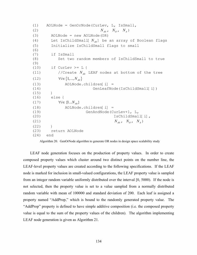
(1) AOLNode = GenOrNode(CurLev, L, IsSmall, (2) AltN , , ON AN ) (3) AOLNode = new AOLNode(OR) (4) Let IsChildSmall[ AltN ] be an array of Boolean flags (5) Initialize IsChildSmall flags to small (6) (7) if IsSmall (8) Set two random members of IsChildSmall to true (9) (10) if CurLev >= L { (11) //Create AltN LEAF nodes at bottom of the tree
(12) { }1,..., Alti N∀ ∈ (13) AOLNode.children[i] = (14) GenLeafNode(IsChildSmall[i]) (15) } (16) else { (17) {1... }Alti N∀ ∈ (18) AOLNode.children[i] = (19) GenAndNode(CurLev+1, L, (20) IsChildSmall[i], (21) AltN , , ON AN ) (22) } (23) return AOLNode (24) end
Algorithm 20. GenOrNode algorithm to generate OR nodes in design space scalability study
LEAF node generation focuses on the production of property values. In order to create
composed property values which cluster around two distinct points on the number line, the
LEAF-level property values are created according to the following specifications. If the LEAF
node is marked for inclusion in small-valued configurations, the LEAF property value is sampled
from an integer random variable uniformly distributed over the interval [0, 5000). If the node is
not selected, then the property value is set to a value sampled from a normally distributed
random variable with mean of 100000 and standard deviation of 200. Each leaf is assigned a
property named “AddProp,” which is bound to the randomly generated property value. The
“AddProp” property is defined to have simple additive composition (i.e. the composed property
value is equal to the sum of the property values of the children). The algorithm implementing
LEAF node generation is given as Algorithm 21.
134

(1) AOLNode = GenLeafNode(IsSmall) (2) AOLNode = new AOLNode(LEAF) (3) if IsSmall (4) PropValue = uniformly distributed random number (5) between 0 and 5000 (6) else (7) PropValue = sample of Gaussian distributed (8) random variable, with mean=100000, (9) stddev = 200 (10) end (11) (12) AOLNode.property(“AddProp”) = PropValue (13) return AOLNode (14) end
Algorithm 21. GenLeafNode algorithm to generate LEAF nodes in design space scalability study
Representing Design Spaces: Propagators and Variables
The design space generation tool was used to create several design spaces of increasing size.
The size of the space is measured by the number of configurations modeled by the space. Figure
36 shows a set of generated design spaces, plotted against their respective sizes on a log scale.
The set of spaces were generated by feeding the parameters 4L = , , , while
varying
10AltN = 3ON =
AN . As can be seen in the plot, the size of the space grows very quickly with respect to
increases in AN . Each space represented in Figure 36 was successfully represented in the finite
domain model. Figure 37 depicts the number of AND-OR-LEAF tree nodes in each design
space model. The number of tree nodes grows linearly with the independent parameter. Since
Figure 36 depicts linear growth of the log of the design space size over the range of the
parameter, it can be concluded that the number of configurations modeled by the design space is
an exponential function of the number of tree nodes.
135

Design Space Size (L=4, Nalt=10, No=3)
0
50
100
150
200
250
300
350
400
1 2 3 4 5 6 7 8 9 10
Na
Spac
e Si
ze (l
og s
cale
)
Figure 36. Size of generated design space, vs. AN
AND-OR-LEAF Tree Size (L=4, Nalt=10, No=3)
0
5000
10000
15000
20000
25000
30000
1 2 3 4 5 6 7 8 9 10
Na
# Tr
ee N
odes
Figure 37. Number of AND-OR-LEAF tree nodes in the generated design spaces
A design space is represented as a set of finite domain variables and constraints. The finite
domain constraints implement the tree structure, while the variables encode the state of inclusion
136
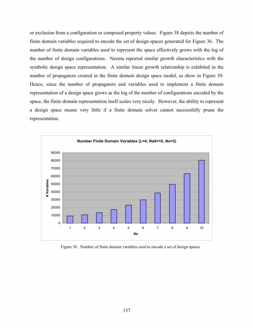
or exclusion from a configuration or composed property values. Figure 38 depicts the number of
finite domain variables required to encode the set of design spaces generated for Figure 36. The
number of finite domain variables used to represent the space effectively grows with the log of
the number of design configurations. Neema reported similar growth characteristics with the
symbolic design space representation. A similar linear growth relationship is exhibited in the
number of propagators created in the finite domain design space model, as show in Figure 39.
Hence, since the number of propagators and variables used to implement a finite domain
representation of a design space grows as the log of the number of configurations encoded by the
space, the finite domain representation itself scales very nicely. However, the ability to represent
a design space means very little if a finite domain solver cannot successfully prune the
representation.
Number Finite Domain Variables (L=4, Nalt=10, No=3)
0
10000
20000
30000
40000
50000
60000
70000
80000
90000
1 2 3 4 5 6 7 8 9 10
Na
# Va
riabl
es
Figure 38. Number of finite domain variables used to encode a set of design spaces
137

Number of Finite Domain Propagators Created (L=4, Nalts=10, No=3)
0
10000
20000
30000
40000
50000
60000
70000
80000
90000
100000
1 2 3 4 5 6 7 8 9 10
Na
# Pr
opag
ator
s C
reat
ed
Figure 39. Growth of the number of finite domain propagators created to model the generated design spaces
Over-, Under- and Critically-Constrained Spaces
A DESERT OCL constraint is translated into a set of finite domain constraints that are
added to the design space model. These additional constraints strengthen the constraint store by
providing additional information (through reducing intervals or binding values to variables).
Adding information to the constraint store implies the potential for propagation. Hence, adding
constraints to the design space model can have the effect of decreasing the time to solution
through the facilitation of propagation. By adding a constraint that provides no “new”
information to the store (i.e. the constraint is already entailed by the store), no propagation
results. This is effectively what happens when a constraint establishes a bound far to the right of
the cluster of composed property values, as discussed in the above section. Large, under-
constrained spaces have a large number of potential solutions. Distribution over large, severely
under-constrained spaces results in an exponential growth in memory usage for a finite domain
constraint solver. This is due to the fact that distribution effectively performs an enumeration of
an exponential space. The finite domain model used in DesertFD is not immune to this
138

characteristic of Mozart. A worst-case scenario for scalability examines how large of an under-
constrained space can be searched by the finite domain design space model.
The following experiments utilize the constraint utilization, best-case search model
described in Chapter III. A single constraint is generated at the root node of the AND-OR-LEAF
tree, which establishes an upper bound on the composed property value at that node. This
constraint is assigned a utilization number, and the solver is instructed to find a solution which
maximizes utilization. This effectively implements a single-solution search. In the worst-case
scenario, the bound established by the constraint is very large and has little effect on the pruning
of the space. Specifically, in the experiment below, the constraint value was set at (the
composed property values ranged from to , thus the bound was set at roughly
an order of magnitude greater than the largest composed property value). Figure 40 shows the
time required to determine a single solution to the finite domain problem modeling a severely
under-constrained design space. Note that the final three design spaces could not be searched
due to lack of virtual memory. Thus, the finite domain approach successfully pruned spaces
containing configurations in this worst-case scenario.
81.0 10×63.0 10× 75.0 10×
18010
Constraint Application Time for Severely Under-Constrained Space (L=4, Nalt=10, No=3)
0
5000
10000
15000
20000
25000
30000
1 2 3 4 5 6 7 8 9 10
Na
Tim
e (m
s)
Figure 40. Time to a single solution for a severely under-constrained design space
139

However, there is a significant difference between the worst-case and the best-case scenario.
The best case scenario with respect to this metric is a space where the application of a constraint
results in significant propagation and elimination of design configurations. Such “near critically-
constrained” spaces are not the general case in design space exploration, but their examination
results in several observations on scalability. The high impact of propagation on the design
space search of the best case scenario significantly reduces memory requirements of the search
and results in much faster search times. Figure 41 depicts the results of the search of a near-
critically constrained design space. Not only are the search times nearly an order of magnitude
better, but spaces of much larger size were able to be searched as well. In this example, a design
space of was pruned in less than 6 seconds. It should be noted that Figure 41 does not
predict the constraint application time of all “critically constrained” design spaces. Research into
phase transitions indicates that constraint satisfaction problems can be constructed which, when
critically constrained, contain very few solutions which are very difficult to find. The results
presented here do not pretend to contradict such findings, due to the fact that the design space
constructed in this example does not exhibit a structure which results in a phase transition (or at
least no phase transition was experimentally discovered).
37710
Constraint Application Time for Near-Critically Constrained Spaces (L=4, Nalt=10, No=3)
0
1000
2000
3000
4000
5000
6000
1 2 3 4 5 6 7 8 9 10
Na
Tim
e (m
s)
Figure 41. Constraint application time for near-critically constrained design spaces
140

The finite domain model scalability varies, depending on how tightly constrained the design
space is. A finite domain model tends to become exponential in memory size as the number of
distribution steps grows. At each distribution step, the space containing the state of the finite
domain search problem is cloned and adjusted according to the distribution algorithm. The
scalability of a finite domain model depends on the number of distribution steps required to
arrive at a solution, as well as the size of the cloned constraint store. Figure 42 compares the
number of distribution steps required to arrive at a solution for the under-constrained and near-
critically constrained design spaces described above. In the near-critically constrained case, the
number of spaces cloned remains fairly constant, whereas for the under-constrained case, the
number of spaces cloned grows linearly. The size of the constraint store is a function of the
number of finite domain variables employed in the model, which as Figure 38 shows, grows
linearly with increasing AN . The increase in distribution steps required to solve the model,
together with the increase in size of constraint store, prevents the pruning of under-constrained
design spaces in this example with AN greater than or equal to 8.
141

Number of Cloned Spaces in Design Space Search (L=4, Nalts=10, No=3)
0
100
200
300
400
500
600
700
800
1 2 3 4 5 6 7 8 9 10
Na
# C
lone
d Sp
aces
Near-Critically Constrained Under-Constrained
Figure 42. Number of space cloned during finite domain evaluation of under-constrained and near-critically
constrained design spaces
The solution of a design space exploration problem becomes increasingly difficult as the
space transitions from a critically-constrained space to a severely under-constrained space.
Figure 43 shows the effect of successively relaxing a constraint on a generated design space. A
single design space with parameters 4L = , 5AltsN = , 3ON = , and 5AN = was generated for this
experiment, and repeatedly solved, using various constraint bounds. This space models roughly
configurations. The smallest composed property value in the space is 3,068,057, while the
largest composed property value is 18,876,151. For this experiment, the space was annotated
with a single constraint, imposing a bound on the root-level composed property value. The value
of this bound was increased over successive executions of the solver. The chart shows both the
constraint application time and the number of cloned spaces utilized during the search. Note that
for constraint bounds lower than the minimum value, the problem becomes an over-constrained
space, and the search fails. All such cases for this space exhibited similar behavior:
approximately 330 ms search time, with no cloned spaces. Similarly, for all constraint bounds
7110
142

significantly above the maximum composed value, the space becomes severely under-
constrained, and all searches result in approximately the same search time (2400 ms) and number
of cloned spaces (366). The chart clearly shows the correlation between constraint application
time and number of distribution steps: an increase in the number of distribution steps correlates
with an increase in the search time.
An interesting search result captured in Figure 43 is the behavior of over-constrained design
spaces. Interval propagation facilitates bounds-checking and evaluation. In the case of the
generated design space, interval propagation was able to establish a lower bound on the
composed property value prior to the commencement of distribution. When the constraint bound
is placed below that lower bound, the constraint solver can immediately determine that the
design space is over constrained by comparing with this bound. By virtue of this comparison,
the search terminates very quickly. However, while this result will be common in many design
space compositions, it cannot be generically stated that DesertFD will always be able to
determine that a space has no solutions without distribution. The use of logical implication in
constraints can lead to the construction of an over-constrained design space, but where interval
propagation cannot determine a bound sufficiently tight so as to detect the infeasibility of the
space.
The severely under-constrained case is also represented in Figure 43. In the case where the
constraint bound is placed well above the maximum composed property value of the design
space, the constraint has no affect on propagation. In the case of this experiment, when the
constraint is placed above the value of the upper bound of the initial interval of the composed
property value of the root node, then the constraint is already entailed by the constraint store, and
has no effect on propagation. In the case of this generated example, interval propagation is able
to determine a tight upper bound to the composed property value at the context of the constraint;
thus the threshold where the constraint bound has an effect is quite close to the maximum
composed property value of the design space.
143

Constraint Application Time over Varying Constraint Bounds
0
500
1000
1500
2000
2500
3000
0.0E+00 5.0E+06 1.0E+07 1.5E+07 2.0E+07 2.5E+07
Cosntraint Bound
Tim
e (m
s)
0
50
100
150
200
250
300
350
400
# C
lone
d Sp
aces
Constraint Application Time Number of Cloned Spaces
Figure 43. Chart showing the constraint application time and number of cloned spaces resulting from the
solution of a single design space whose constraint bound is successively relaxed
Figure 43 illustrates a fairly sharp transition from minimum search time to search times
closer to the maximum time. However, a “zoomed in” examination of a section of this graph
illustrates some interesting relationships during this transition. The left-most points in the
dataset plotted in Figure 44 correspond to the over-constrained case, where the constraint bound
is set below the minimum composed property value in the design space. As can be seen in the
figure, as the constraint bound increases, the search time and number of cloned spaces required
to converge at a solution increases, until peaking between the constraint bound values of
and . The search time then falls, and then falls again sharply just after the
bound value of . This is followed by a second cycle of the search time rising and then
falling. The plot illustrates the fact that search performance is not simply a linear relationship
with the constraint bound over the transition from an over-constrained to severely under-
constrained space. Depending on the structure of the space and the property values involved,
some design spaces may converge to a solution more quickly than others. The cyclic nature of
63.1 10× 63.15 10×63.15 10×
144

the data depicted in Figure 44 suggests a transition from a difficult-to-solve design space to an
easy-to-solve design space.
Constraint Application Time (L=4, Nalts =5, No=3, Na=3)
0
100
200
300
400
500
600
700
800
900
1000
3.05E+06 3.10E+06 3.15E+06 3.20E+06 3.25E+06 3.30E+06 3.35E+06
Constraint Bound
Tim
e (m
s)
0
50
100
150
200
250
# C
lone
d Sp
aces
Constraint Satisfaction Time Number of Cloned Spaces
Figure 44. Chart showing a zoomed-in view of a portion of Figure 43, illustrating the transition from an over-
constrained space to under-constrained space.
Width vs. Depth
The design space generation tool can be used to construct spaces that vary by width as well
as by depth. The above experiments that show a change of design space size have varied only
the number of AND-decomposed children of an AND node through the AN parameter.
Effectively this widens the AND-OR-LEAF tree by supplying each AND node with more
children. An analysis was performed on the sensitivity of the design space scalability to tree
structure by varying the width through the parameter instead of ON AN , and by varying the
depth instead of the width.
The number and position of OR nodes in the design space structure control the orthogonality
of the space. Figure 45 shows how the size of a generated space grows as the number of OR-
145

decomposed children of an AND node is increased. In this case, the number of AND-node
children of OR nodes is fixed at 10, while the quantity of AND-decomposed children of AND
nodes is fixed at 3. The depth of the tree is set to 4, as in the previous experiments. It can be
seen that the log of the number of configurations modeled in the space is linear in the number of
OR node children of AND nodes. By way of comparison, the parameter set , 4L = 10AltsN = ,
, results in a space modeling configurations, while the parameter set 3AN = 8ON = 16810 4L = ,
, , results in configurations. The generated space grows faster
with
10AltsN = 8AN = 3ON = 22310
AN than with . ON
Design Space Size (L=4, Nalts=10, Na=3)
0
20
40
60
80
100
120
140
160
180
1 2 3 4 5 6 7 8
No
Spac
e Si
ze (l
og s
cale
)
Figure 45. Chart depicting the change in size of design space against the number of OR node children of an
AND node.
The scalability of the finite domain model is affected by the structure of the space. By
increasing the number of OR-node children of an AND node, the generated space contains many
more OR nodes. The propagation model for AND node finite domain variables is much stronger
than the model for OR nodes. Therefore, a highly orthogonal design space must rely on
distribution more than a space composed more of AND nodes. The increased reliance on
distribution impacts scalability, as described previously. Figure 46 shows the performance of the
146

constraint solver on highly orthogonal, severely under-constrained design spaces. The search of
the space generated for parameter 7ON = did in fact terminate successfully, but exhibited a very
long execution time (over 400 seconds), due to virtual memory consumption which exceeded the
RAM capacity of the benchmark machine. The search performance grows linearly in the number
of cloned spaces, but the execution time grows super-linearly. The data shows poorer scalability
for highly orthogonal design spaces.
Constraint Application Time for Highly-Orthogonal, Severely Under-Constrained Design Spaces (L=4, Nalts=10, Na=3)
0
5000
10000
15000
20000
25000
0 1 2 3 4 5 6 7 8 9
No
Tim
e (m
s)
0
100
200
300
400
500
600
# C
lone
d Sp
aces
Constraint Application Time Number of Cloned Spaces
Figure 46. Chart showing the constraint solver performance on increasingly orthogonal design spaces
An examination of search performance for deep, as opposed to wide, design spaces was also
performed. For this experiment, several design spaces were generated with the following
parameter set: , , 2AltsN = 2AN = 1ON = , and by varying . Figure 47 plots the log of the
generated design space size against the maximum depth of the tree. It can be seen that the log of
the size of the space is a super-linear function of the depth of the tree.
L
147

Design Space Size (Nalts = 2, Na = 2, No=1)
0
50
100
150
200
250
4 5 6 7 8 9
L
Des
ign
Spac
e Si
ze (l
og s
cale
)
Figure 47. Chart showing the sizes of design spaces generated by varying the depth of the AND-OR-LEAF tree
The performance of the design space search over deep trees is given in Figure 48. Both
dependent variables are plotted in log scale. While both the search time and number of cloned
spaces exhibit exponential growth, prior to memory exhaustion occurring at tree depth of 9, the
observed execution performance is acceptable. The design space generated , for example,
is successfully searched in approximately 14 seconds, involving 834 distribution steps. An
observation of the performance of the deep design spaces is that they require more distribution
steps in order to converge on a solution, when compared to wide design spaces. Chapter III
describes the propagation model for both select variables and for property composition. While
the propagation model is constructed to support upward and downward propagation, values,
especially those of the boolean select-variables, propagate easily across the children of a node,
but downward propagation halts at an OR node.
8L =
148

Constraint Applcation Performace over Varying Depth Trees (Nalt=2, Na=2, No=1)
0
0.5
1
1.5
2
2.5
3
3.5
4
4.5
4 5 6 7 8 9
L
Tim
e (lo
g sc
ale,
ms)
0
0.5
1
1.5
2
2.5
3
3.5
# C
lone
d Sp
aces
(log
sca
le)
Constraint Application Time Number Cloned Spaces
Figure 48. Chart showing the performance of constraint application to increasingly deep design spaces
Experiment Evaluation and Applicability
The above experiments illustrate the degree of scalability of the finite domain model for
design space exploration employed by DesertFD. This section comments on the fairness of the
experiments in establishing the scalability, and notes limitations in the tests, prior to the
summary of findings and conclusions presented in the next section.
The design space generation utility produces only full, dense design spaces. While for some
cases, this structure represents a worst-case scenario, a more randomly generated design space
structure may potentially reflect actual design spaces. Further, only one DESERT OCL
constraint is generated and applied to the space. Rarely is it the case that a single constraint will
drive the design space exploration. However, for the purpose of illustrating scalability, a single
constraint does suffice. Also, the fact that a single constraint is applied renders the use of the
best-case search for the maximization of constraint utilization as wasted effort. Specifically,
once a solution to the constraint is found, the algorithm continues the search in order to prove
149
that a better value cannot be found. This may result in a larger number of distribution steps than
would otherwise be needed.
The generation of LEAF level property values such that composed property values are
separated into distinct clusters affects the difficulty of the design space exploration problem.
When a constraint bound is placed below the values of the majority of the higher cluster, interval
propagation facilitates the removal of a large number of nodes from the design space prior to the
first distribution step. While this illustrates the power of the propagation model, the complexity
of the problem is reduced significantly prior to distribution.
When compared to the symbolic design space representation method employed by Neema,
the experiments described here lack in a few aspects. The OBDD representation encodes all
solutions in the design space. The experiments here employ a best-case search, where only one
solution is calculated. This approach is employed in order to avoid the exponential memory
growth associated with an all-solutions search across an under-constrained search problem.
Scalability Conclusions
The data support several conclusions. First, the cause of scalability limitations is related to
distribution. Distribution is measured by the number of times the solver clones a space during
the search. When the number of distribution steps can be kept small and bounded, the finite
domain representation of the design space scales very well. The worst case situation for the
finite domain representation of a design space is a severely under-constrained space. Search of
such spaces rely heavily on distribution, and thus encounter scalability problems. The
experiments presented in this chapter illustrate the successful representation and pruning of
severely under-constrained design spaces modeling up to configurations in the case of very
deep design spaces, configurations for highly orthogonal spaces, and configurations
for wide, but less orthogonal spaces. The experiment examining scalability for critically
constrained spaces illustrates the pruning of a design space modeling configurations.
871014010 18010
37710
These experiments illustrate the power of the propagation model implemented for design
space exploration. The finite domain model described in Chapter III establishes a single Boolean
finite domain variable for every node in the AND-OR-LEAF tree. Further, a finite domain
variable is allocated for every node in the tree for each type of property assigned to the tree. The
property variables assigned to interior tree nodes model composed property values. Without
150

propagation, the solution of a finite domain model would require sufficient distribution steps to
establish values for each of the select variables and each of the property variables. Propagation
facilitates the binding of values to some of these variables based on the values of other variables.
In the above experiments, the largest number of distribution steps needed to obtain a solution to a
space was 834, with the parameter set 2AltsN = , 2AN = , 1ON = , and 8L = . This space results
in an AND-OR-LEAF tree consisting of 5274 nodes, and models configurations. As
mentioned in the discussion above, it represents the worst case encountered for propagation, due
limitations on vertical propagation. However, even with limited propagation, the ratio of
distribution steps to finite domain variables modeling tree node values is roughly 0.08.
8610
Neema reported scalability concerns with the application of arithmetic constraints to the
symbolic design space representation. He illustrated the limitation in scalability to design spaces
modeling up to configurations. All experiments in this section have applied arithmetic
constraints, where the worst-performing worst-case scenario scaled to at least
configurations. The scalability of the BDD approach for logical and relational constraints,
coupled with the ability to prune large, highly under-constrained spaces, supplies the impetus
behind the unification of the two techniques in the hybrid design space exploration technique.
1510
8610
Conclusions
DesertFD is an integrated design space exploration toolset which builds on the structure of
DESERT. Neema developed a highly scalable design space model and exploration techniques
based on a binary encoding and an OBDD-based symbolic design space representation.
DesertFD extends DESERT through the translation of the design space model into a finite
domain constraint representation. The finite domain representation is translated and dynamically
instantiated in the Mozart engine, where best-case branch and bound search is used to determine
a solution which best meets utilization criteria specified by the user. The best-case solution is
returned to the user in the DESERT XML syntax. DesertFD integrates the OBDD-based design
space exploration tool with the finite domain constraint solver by translating a pruned BDD-
based design space into a logic function, which is then expressed as a finite domain constraint
expression tree. This expression tree captures the dependencies derived during BDD-based
pruning, and applies those dependencies to the finite domain-based search. Any constraint
which is determined to potentially cause scalability problems in the BDD representation is
151

marked for application in the finite domain constraint representation. All other constraints are
passed to the BDD for potential selection and application by the user. Once the BDD-based
pruning is terminated, the representation is translated into a finite domain representation and
transmitted to the Oz Engine for finite domain search.
A quantitative analysis of the scalability of the finite domain representation of design spaces
has been presented. The finite domain representation has been shown to scale to large numbers
of design configurations for various types of design space composition. The issue of the degree
of constraint of a design space has been discussed, including an illustration of the best-case
situation for design space exploration: where a constraint bound is sufficiently close to a solution
value so as to make the search trajectory obvious to the distribution algorithm. In such cases,
very little distribution is needed to determine a solution to the finite domain model, allowing
very large (up to configurations) design spaces to be pruned. 37710
152

CHAPTER VI
CONCLUSIONS AND FUTURE WORK
Design space exploration is an important area of research in the field of embedded systems
design. Design is a process of intelligently weighing tradeoff decisions. Design space
exploration formalizes this concept of tradeoff evaluation through the application of formal
analyses to design compositions. Design space exploration strives to determine a design or small
set of designs which meet formally specified criteria. Several tools have been developed and
described in the literature which implement design space exploration algorithms tailored to
various classes of applications. Each tool takes a different approach with differing metrics and
degrees of success. The variety of tools and approaches indicates the difficulty of the design
space exploration problem, and that, arguably, no single “best” solution approach exists. Rather,
hybrid design space exploration approaches must be examined, which integrate and unify
successful exploration techniques. This dissertation has examined the development of such a
hybrid exploration technique, embodied in a tool called DesertFD.
Summary of Findings
DesertFD is built on DESERT, the design space exploration tool developed by Neema.
DESERT offers a domain-independent design space modeling specification which facilitates the
specification of a design space as an attributed AND-OR-LEAF tree. Constraints capture
relationships between nodes in the tree, and properties quantified over the tree. Design space
exploration in DESERT is a constraint satisfaction problem, where the constraints encode the
non-functional requirements of the design. DESERT implements the constraint satisfaction
problem using a symbolic representation of the space and constraints, based on Ordered Binary
Decision Diagrams. The OBDD-based representation of the design space has been found to be
highly scalable, except when pruning operations involve arithmetic operations.
DesertFD leverages the domain-independent design space modeling specification of
DESERT, but translates the design space exploration and constraint satisfaction problem into a
finite domain constraint representation. An efficient finite domain propagation model has been
developed to implement the AND-OR-LEAF tree semantics, as well as property composition
153

functions for the various classes of property composition supported by DESERT. DESERT OCL
constraints have been translated into finite domain constraints as well. A customized distribution
algorithm has been implemented to facilitate a complete finite domain design space search.
DesertFD extends the design space modeling specification of DESERT with the Property
Composition Language. The set of property composition functions supported by DESERT is
limited to a small set of functions which implement a single composition operation, over a single
property. The Property Composition Function facilitates the specification of arbitrarily complex
mathematical functions for modeling property composition. PCL functions may reference
properties other than the property type specified as the result of the composition. Non-linear
mathematical operations are also supported, including integer division and modulus, and
exponentiation. The PCL specification of properties facilitates a parametric specification of
property composition, where LEAF nodes need not be supplied with simple numerical data for
property values. Rather, value computation can be left as a function of a PCL specification.
DesertFD provides a translator for PCL which maps PCL specifications into a finite domain
representation, leveraging the AND-OR-LEAF finite domain representation.
DesertFD integrates the OBDD-based symbolic constraint satisfaction engine implemented
in DESERT with the finite domain constraint search described above. Due to scalability
considerations of the OBDD space representation with respect to arithmetic operations, the set of
constraints supplied in the design space model is sorted based on whether the application of the
constraint will result in an explosion of BDD nodes in the symbolic representation. DesertFD
then prunes the design space using the symbolic approach of DESERT, and translates the
resulting pruned BDD into a Boolean logic expression. This expression is translated into a set of
finite domain constraints, together with the design space specification and the remaining OCL
constraints. The finite domain constraints are fed to the Oz Engine dynamically through a TCP
connection. When the finite domain constraint solver encounters a solution to the pruned design
space, it returns the solution to the user.
The scalability of the finite domain constraint representation of the design space has been
quantitatively evaluated. The design space representation has been found to be highly scalable
across several classes of generated design spaces. Scalability limitations in the finite domain
representation are encountered when the number of distribution steps required to arrive at a
154

solution becomes unbounded. However, where the number of distribution steps can be kept
bounded, the finite domain representation is highly scalable.
Future Work
The major result of this research is an integrated toolset implementing design space
exploration through symbolic pruning and constraint satisfaction. There are several potential
directions that can build on the work described in this dissertation, outlined in the sections
below.
Design Space Modeling
The domain-independent design space modeling specification supported by DESERT and
DesertFD is limited by the use of enumeration of design choice. Often, a design space is more
naturally modeled using a parametric approach. Currently, OR nodes model design choice. All
potential outcomes of a design choice must be enumerated and explicitly included in the design
space definition. Certain classes of design spaces are more elegantly modeled with a parametric
approach, where parameters embody design choice. Parametric modeling could also be used to
encode the compositional structure of the space.
An issue has arisen when attempting to model the mapping of an application onto
reconfigurable resources using the current DESERT modeling specification. The current
approach for modeling resource allocation involves the creation of a property to represent the
resource binding, and the specification of the domain of that property to be the set of resources to
which the object may be bound. For a configurable resource, an enumeration of the potential
resource bindings can become prohibitively expensive, if the space of configurability is large.
Techniques are needed to facilitate the representation of property domains as spaces themselves,
without requiring explicit enumeration.
The representation of shared resources can be complicated in the design space model. While
the current resource allocation model facilitates the representation of shared resources (simply
through the binding of multiple elements to the same resource), property composition functions
which depend on the characteristic of shared resources are difficult to specify. An extension of
the design space model to more explicitly represent shared and sharable resources is warranted.
155

Scalability Improvements with DesertFD
The scalability of the hybrid search approach offered by DesertFD should be examined and
improved. The scalability analysis of the finite domain design space model illustrated the
inverse relation between scalability and number of distribution steps. An examination of
heuristics to facilitate increased scalability in the finite domain search is warranted. Mozart
offers significant flexibility in guiding distribution and search through heuristics. Multiple
heuristics have been reported in the literature, and should be evaluated and integrated where
appropriate in the finite domain search.
DesertFD implements a simple integration of the finite domain constraint solver with the
symbolic BDD-based constraint satisfaction tool. Future research should quantitatively
characterize the benefits and drawbacks of each solution technique, and examine the possibility
of a more dynamic, interactive hybrid search. Such a dynamic approach could involve the
translation of the search problem from a finite domain specification back into a BDD-based
specification for further refinement. The goal of tighter integration is to improve the scalability
of the search.
Solver Integration
DesertFD has outlined a hybrid design space exploration technique, involving the OBDD-
based symbolic representation of DESERT and the finite domain constraint representation
presented in this dissertation. As discussed previously, the number of approaches identified in
the literature for modeling and solving embedded system design space exploration problems not
only justifies, but practically implies the need for hybrid search approaches. A future direction
for research with design space exploration tools involves the integration of other modeling
techniques and solvers. Specifically, as benchmarks indicate performance benefits of
pseudoboolean solvers when compared to finite domain solvers, a pseudoboolean solver could be
integrated into the design space exploration tool suite.
Arguably more pressing, however, is the need to integrate a solver which supports floating
point operations. This need is highlighted by an attempt to model reliability as a composed
property. Reliability is a probabilistic measure of the likelihood of failure of a component or
system. Reliability in some systems can be modeled as a composable property, with
multiplicative composition. However, due to the probabilistic nature of reliability values, an
156

integer representation of the property composition function necessarily involves explicit
quantization. In applications where precision is critical, an implementation of fixed-point
arithmetic would be necessary to represent with high accuracy the composition operations. The
integration of a solver capable of managing floating point calculations mitigates the tedium of
managing fixed point arithmetic in the integer-based finite domain solver. Candidate solvers
include an MILP-based solver or CLP(R).
Design space modeling in DESERT and DesertFD facilitates the pruning of spaces based on
composed structural properties of a design. These properties abstract away the complexities of
dynamic interactions at the behavioral level of design, by lumping quantitative estimates of
worst-case or average-case behavior into single parameters. Often, these worst-case estimates
are highly pessimistic, resulting in poor pruning of the design space. The development and
integration of behavioral estimation models into the design space exploration flow could be
explored in order to improve pruning. However, such approaches need to be tempered with data
on the size of the design spaces, due to the fact that dynamic behavioral estimation tends to be
more computationally intensive, and can hamper the scalability of the search.
A by-product of solver integration should be increased hybridization of the design space
search. The justification for hybridization stipulates that each good search technique
demonstrates its own strengths, but also has its drawbacks. As solvers are integrated,
quantitative analyses must be performed to characterize the behavior of the solver across
different classes of datasets. Hybridization seeks to exploit each solver in such a way so as to
glean the benefits of what each solver does well, and sidestep areas where a solver exhibits poor
performance. Further, the task of mapping a problem specification into the solver domain must
be benchmarked as well in order to facilitate a cost/benefit analysis of dynamically mapping a
design space representation onto a different solver.
Embedding Exploration
Embedded architectures are becoming larger and more complex. Often, architectures
facilitate structural reconfiguration to allow a better fit of an application computation on the
architecture’s resources. Currently, the topic of dynamic reconfiguration is an open topic of
research. Design space exploration could be used to traverse the space of potential application-
to-architecture mappings at runtime. However, current approaches utilized in DESERT and
157

DesertFD are likely poor candidates to implement such exploration. The on-line exploration
algorithms must be deterministic if they are to be integrated into a real-time embedded system.
An interesting research direction is the amalgamation of off-line static design space analysis and
pruning with on-line exploration. The goal of the off-line search is to prune the full design space
into a small subspace which can then be pruned and explored deterministically at runtime. The
goal is complicated by the need to allow sufficient variance in the on-line design space so as to
facilitate dynamic optimization.
Tool Integration
The domain-independent nature of DesertFD facilitates its use across a wide variety of
applications and application domains. Ongoing research into Model-Integrated Computing
[83][84] (MIC) seeks to facilitate the rapid development of domain-specific modeling
environments for use in system design and analysis. In many such application domains, the
process of design implies the exploration of a design space. DesertFD can be integrated into the
toolflow of the domain-specific modeling environment through semantic translation. Ongoing
research into the specification of model-based translators has developed techniques to specialize
domain-independent model-translation interfaces and APIs into domain-specific interfaces [85].
Tools and techniques can be explored which facilitate the easy integration of DesertFD into
model-integrated computing-based toolflows. Specifically, the PCL offers several built-in
functions to facilitate access to properties and other context-specific information. Tools can be
developed which specialize the PCL with domain-specific information relating concepts in a
domain-specific language to the domain-independent PCL functions.
158

Appendix A
PCL LEXICAL ANALISYS SPECIFICATION
%{ #include <stdlib.h> #include <string.h> void handleStrCnst(const char *in, char **out); %} %% "+" {return(PLUS);} "-" {return(MINUS);} "*" {return(STAR);} "/" {return(FSLASH);} "%" {return(PCENT);} "<" {return(LT);} "<=" {return(LEQ);} ">" {return(GT);} ">=" {return(GEQ);} "==" {return(EQEQ);} "!=" {return(NEQ);} "!" {return(BANG);} "&&" {return(ANDAND);} "||" {return(OROR);} "=" {return(EQ);} "," {return(COMMA);} "(" {return(LPAREN);} ")" {return(RPAREN);} "." {return(DOT);} "[" {return(LBRACK);} "]" {return(RBRACK);} "{" {return(LBRACE);} "}" {return(RBRACE);} ";" {return(SEMICOLON);} "if" {return(IF);} "then" {return(THEN);} "else" {return(ELSE);} "elseif" {return(ELSEIF);} "return" {return(RETURN);} "function" {return(FUNCTION);} "var" {return(VAR);} "list" {return(LIST);} "property" {return(PROPERTY);} \"[^\"]*\" {handleStrCnst(yytext, &(yylval.sval));return(STRCNST);} [a-zA-Z]([a-zA-Z0-9_])* {yylval.sval=strdup(yytext); return(IDENTIFIER);} -?[0-9]+ {sscanf(yytext, "%i",(yylval.ival)); return(DECINT);} \n " " \t %%
159

void handleStrCnst(const char *in, char **out) { int len; if(in[0] == '\"') *out = strdup(&in[1]); else *out = strdup(in); len = strlen(*out); if((*out)[len-1] == '"') (*out)[len-1] = '\0'; }
160

Appendix B
PCL CONTEXT-FREE GRAMMAR SPECIFICATION
%{ int yylex(void); %} %token PLUS %token MINUS %token STAR %token FSLASH %token PCENT %token BANG %token LT %token LEQ %token GT %token GEQ %token EQEQ %token NEQ %token ANDAND %token OROR %token EQ %token COMMA %token LPAREN %token RPAREN %token DOT %token LBRACK %token RBRACK %token LBRACE %token RBRACE %token SEMICOLON %token IF %token THEN %token ELSE %token ELSEIF %token RETURN %token FUNCTION %token VAR %token LIST %token PROPERTY %token STRCNST %token IDENTIFIER %token DECINT %left PLUS MINUS STAR FSLASH PCENT ANDAND OROR %nonassoc LT LEQ GT GEQ EQEQ NEQ %% prog: funcList ; funcList: func
161

| func funcList ; func: prototype body ; prototype: PROPERTY IDENTIFIER formalParams | FUNCTION VAR EQ IDENTIFIER formalParams | FUNCTION LIST EQ IDENTIFIER formalParams | FUNCTION IDENTIFIER formalParams ; formalParams: LPAREN formalParamList RPAREN ; formalParamList: formalParam COMMA formalParamList | formalParam | /*nothing*/ ; formalParam: varDecl | listDecl ; varDecl: VAR IDENTIFIER ; varDeclInit: varDecl EQ opExpression ; listDecl: LIST IDENTIFIER ; listDeclInit: listDecl EQ opExpression | listDecl EQ LBRACK varList RBRACK ; varList: varList COMMA IDENTIFIER | IDENTIFIER | /*nothing*/ ; body: LBRACE statementList RBRACE ; statementList: statement | statement statementList ; statement: declStatement SEMICOLON | opStatement SEMICOLON | controlStatement SEMICOLON | returnStatement SEMICOLON ; declStatement: varDeclInit | varDecl | listDeclInit | listDecl ; controlStatement: ifStatement ; ifStatement: ifPart elseifList elsePart ; ifPart: IF conditionExpr THEN body ; elseifList: elseifPart elseifList | /*nothing*/ ; elseifPart: ELSEIF conditionExpr THEN body ;
162

elsePart: ELSE body | /*nothing*/ ; conditionExpr: LPAREN opExpression RPAREN ; returnStatement: RETURN opExpression ; opStatement: assignStatement | callStatement ; callExpression: call DOT callExpression | call ; callStatement: callExpression ; call: IDENTIFIER LPAREN actParams RPAREN ; actParams: actParamList |/*nothing*/ ; actParamList: actParam COMMA actParamList | actParam ; actParam: callExpression | operand ; assignStatement: IDENTIFIER EQ opExpression ; opExpression: opExpression PLUS opExpression | opExpression MINUS opExpression | opExpression STAR opExpression | opExpression FSLASH opExpression | opExpression PCENT opExpression | opExpression ANDAND opExpression | opExpression OROR opExpression | opExpression EQEQ opExpression | opExpression NEQ opExpression | opExpression LT opExpression | opExpression LEQ opExpression | opExpression GT opExpression | opExpression GEQ opExpression | opParenExpr | operand | BANG operand | callExpression ; opParenExpr: LPAREN opExpression RPAREN | MINUS LPAREN opExpression RPAREN ; operand: IDENTIFIER | MINUS IDENTIFIER | DECINT | STRCNST ; %%
163

APPENDIX C
CASE STUDY: EMBEDDED AUTOMOTIVE SOFTWARE
The automotive industry currently seeks to develop robust, reliable, fault-tolerant embedded
implementations of x-by-wire applications. X-by-wire refers to the replacement of mechanical
or hydraulic systems in the vehicle with computer-based systems. One such application is called
steer-by-wire, where the traditional mechanical/hydraulic connection between the steering wheel
of a vehicle and its wheels is replaced by an electronic connection between sensors and actuators.
X-by-wire applications present several design challenges, due to the impact of strict safety and
reliability requirements on the embedded control system. This appendix examines the tradeoff
between increased application reliability brought through redundancy, and the hard
schedulability requirements imposed on the system. DesertFD is used to model the tradeoff
decision and its impact on resource allocation as a design space exploration problem.
Specifically, the space of alternative application-to-architecture mappings is captured as a design
space, and is analyzed over reliability and schedulability metrics.
Steer-By-Wire Application
Steer-by-wire utilizes sensors and actuators to facilitate the steering control of a vehicle.
Typically, steering in a passenger vehicle is implemented through a physical connection between
the steering column and the rack and pinion system connected to the wheels. The rack and
pinion is responsible for converting adjustments to the steering wheel angle into lateral
adjustments to wheel position. Hydraulics have been introduced into the steering system to
implement power steering, facilitating a reduction in the force required on the steering wheel to
implement a turn. Steer-by-wire seeks to replace this physical connection between the steering
column and the rack and pinion with a reliable, fault-tolerant embedded computer system.
Sensors are placed on the steering column to capture change-of-direction input from the user.
Actuators are placed on the rack and pinion to allow the computer system to control lateral wheel
motion. The embedded computer system implements an intelligent feedback control algorithm,
which not only facilitate steering changes based on user input, but also potentially increases the
safety of the vehicle through explicit detection and management of faults.
164
The integration of embedded processing in the vehicle control platform facilitates new
approaches to safety, reliability and fault-tolerance in vehicle design. Steer-by-wire, for
example, takes not only the current state of the vehicle and the user-specified direction change
requests, but also uses other information gleaned from sensors throughout the vehicle. Sensors
provide information on the current position of all four wheels, the state of the motor, pitch, yaw
and roll of the vehicle and several other relevant metrics. This information is fed to the control
algorithm in order to determine the proper actuation to apply. The control algorithms are
designed to react to faults so as to maximize the safety of the vehicle occupants. In the presence
of faults, the system enters a degraded mode of operation. In the presence of serious faults, a
mechanical steering system backup is enabled.
Typical steer-by-wire applications utilize sensors and actuators scattered throughout the
vehicle. The embedded computing platform consists of several ECUs (Electronic Control Units)
connected through a fault-tolerant bus. A typical ECU contains a microprocessor, memory and a
bus interface controller. Sensors and actuators interface directly to an ECU. The physical layout
of the embedded platform typically relates to the location of the sensors. The steer-by-wire
algorithm utilizes position information gleaned from sensors at each of the four wheels. The
application also implements a supervisory control algorithm which is responsible for analyzing
the current fault state of the system and for determining whether and when to disengage actuators
and engage mechanical backups. Figure 49 shows the embedded platform used in this design
space analysis. The platform consists of five ECUs, one for each wheel in the vehicle, and one
“supervisor” ECU. Each ECU is connected to a set of sensors and actuators. Each wheel ECU is
interfaced to wheel position sensors, which sense the absolute and relative wheel position. Each
wheel ECU is interfaced to an actuator which implements the torque on the rack and pinion
responsible for turning each wheel. Sensors are placed on the steering wheel to sense torque and
handwheel position. The torque sensor is interfaced to ECU F1, while ECUs F2 and RL are
interfaced to handwheel position sensors. In order to give the vehicle operator a sense of
connectivity with the road, feedback is provided to the steering handwheel through the Steering
Feedback Torque actuator interfaced to ECU F1.
165

Figure 49. Embedded automotive computing platform for steer-by-wire application
The steer-by-wire application examined in this case study seeks to implement four-wheel
by-wire steering, and explicitly manages system faults. The algorithm consists of a set of data
dependent, concurrent tasks. The application is modeled as a directed dataflow graph, where the
nodes in the graph represent tasks and edges represent signals, or information that is
communicated between tasks. The task model does not support queuing of signals between
tasks. Each task is annotated with metadata describing the worst-case execution time for the
task. Since all ECUs in this study contain equivalent microprocessors, the worst-case execution
time of a task does not depend on resource allocation. All tasks in the application have the same
five millisecond deadline. When a task executes, it consumes the signals on which it depends,
performs its computation, and produces the output signals which it sources. A real-time
operating system on each ECU is responsible for executing all tasks mapped to the ECU such
that no task misses a deadline.
166

Input data to the application is received through sensors. The steer-by-wire application is
coupled with other applications in a real vehicle environment. These other applications provide
the steer-by-wire application with real-time processed information generated from other sensors
which are not part of the steer-by-wire platform. These data that are received from other
applications as inputs to the steer-by-wire application are modeled as sensors in this analysis,
even though they are not necessarily generated from hardware sensors. Examples of such data
include the current vehicle speed and the pitch, yaw and roll of the vehicle. Just as with real
sensors, these virtual sensors are assumed to be bound to individual ECUs, modeling the location
in the processing network where the relevant data is held.
Figure 50 depicts the steer-by-wire application analyzed in this study. Each box represents a
logical collection of tasks. Edges in the graph model signals. The ProcessPosition task is
responsible for sampling the position sensors associated with each wheel to determine the current
state of the wheel. The ProcessSteeringWheelData task is responsible for determining
inputs from the user by reading the steering wheel angle and position sensors. Sensor data is
analyzed by the task and compared against thresholds in order to detect anomalies due to sensor
faults. The fault information is passed to the FaultDIR task, which implements fault detection,
isolation and recovery. The FaultDIR task takes the sensor fault information from the steering
wheel and wheel sensor tasks, as well as information on wheel motor temperature, in order to
determine whether the vehicle has encountered a fault. On the detection of a fault, the task
attempts to isolate the fault and apply appropriate recovery measures. Recovery involves the
communication of the fault state of the vehicle to the supervisor and feedback controller, as well
as the communication of a fail-safe steering state to the actuators. The Supervisor is
responsible for monitoring the state of the vehicle to determine if a mechanical steering backup
should be engaged. The Supervisor is implemented as a triple-redundant module with voting
between replicated nodes, so as to increase fault-tolerance. The feedback controller implements
the control algorithms for the steer-by-wire system, where the sensor information is used
together with the fault mode (degraded vs. normal) to determine a set of commands to send to the
actuators. The Actuation task is responsible for converting actuation commands calculated
by the controller into valid torque outputs to the actuators connected to the vehicle rack and
pinion modules to implement a change in vehicle direction. Actuation also produces a force
167
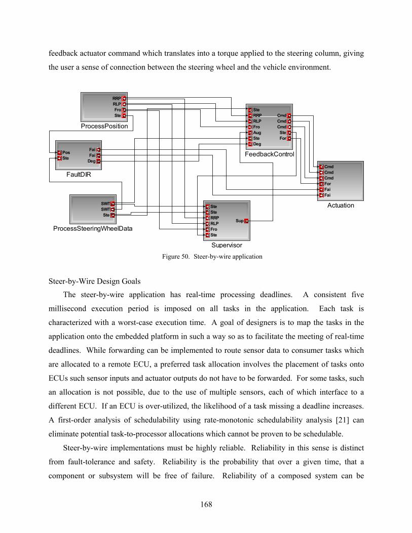
feedback actuator command which translates into a torque applied to the steering column, giving
the user a sense of connection between the steering wheel and the vehicle environment.
RRPRLPFroSte
ProcessPosition
PosSte
FaiFai
Deg
FaultDIR
SteRRPRLPFroAugSteDeg
CmdCmdCmdSteFor
FeedbackControl
SteSteRRPRLPFroSte
Sup
Supervisor
CmdCmdCmdForFaiFai
ActuationSWTSWTSte
ProcessSteeringWheelData
Figure 50. Steer-by-wire application
Steer-by-Wire Design Goals
The steer-by-wire application has real-time processing deadlines. A consistent five
millisecond execution period is imposed on all tasks in the application. Each task is
characterized with a worst-case execution time. A goal of designers is to map the tasks in the
application onto the embedded platform in such a way so as to facilitate the meeting of real-time
deadlines. While forwarding can be implemented to route sensor data to consumer tasks which
are allocated to a remote ECU, a preferred task allocation involves the placement of tasks onto
ECUs such sensor inputs and actuator outputs do not have to be forwarded. For some tasks, such
an allocation is not possible, due to the use of multiple sensors, each of which interface to a
different ECU. If an ECU is over-utilized, the likelihood of a task missing a deadline increases.
A first-order analysis of schedulability using rate-monotonic schedulability analysis [21] can
eliminate potential task-to-processor allocations which cannot be proven to be schedulable.
Steer-by-wire implementations must be highly reliable. Reliability in this sense is distinct
from fault-tolerance and safety. Reliability is the probability that over a given time, that a
component or subsystem will be free of failure. Reliability of a composed system can be
168

calculated from the reliability metrics of the subsystems. Reliability theory [86] dictates that for
a system composed such that if any single subsystem fails, then the system as a whole fails, the
system is said to be serially composed. Assuming that the failure of a subsystem is an
independent event from all other subsystems, the probability of reliable operation of a serially-
composed system can be calculated as the product of the probability of reliable operation of each
subsystem. The multiplicative nature of reliability calculations requires the composition of
highly reliable subsystems in order to produce a reliable system.
The reliability of a system can be improved through parallel composition. Parallel
composition introduces redundancy into the system. In a parallel composition, the composed
system is deemed to be reliable if at least one of the redundant subsystem instances is
functioning properly. Redundancy can be introduced into the steer-by-wire system through
replication and voting. N-way redundancy is implemented by replicating a task N times in the
task graph. The inputs to the task are replicated N times by a splitter node. The outputs of each
replicated task are sent to a voting task, which produces a single output based on a majority-rule
comparison of inputs received from replicated tasks. The splitter and voting tasks are assumed to
always be reliable. Figure 51 depicts a triple-redundant implementation of a task T1, where
tasks T1_1, T1_2, and T1_3 are identical replications of each other.
T1_1
T1_2
T1_3
Splitter Voter
T1
Figure 51. Triple-redundant implementation of task T1
The composed reliability of the replicated system reflects the voting scheme used. In the
case of majority-rule, the reliability is calculated as the probability that a simple majority of the
169

tasks will succeed. In the case of triple redundancy, reliability can be calculated as follows. Let
be the probability that a task t operates as intended by the designer. The reliability of a triple-
redundant parallel configuration task t is then the probability that either all three replicated
instances will agree, or that any two will agree while one fails. Noting that the sum of the
probability of success and the probability of failure equate to unity, equation (35) gives the
reliability composition function for a triple-redundant voting parallel configuration.
ts
(35) 23 3 2t treliability s s= − 3
t
An analysis of equation (35) reveals that the triple-redundancy increases reliability only when
. The computation again assumes that the failure modes of the redundant tasks are
independent.
0.5ts ≥
For the purposes of this study, the task of the designer is to determine a mapping of
application tasks onto the set of available resources such that the resulting application is
schedulable, and sufficiently reliable. Where the reliability of the application is deemed
insufficient, the designer can select tasks in the task graph to implement in a replicated parallel
configuration, as discussed above. Figure 52 models a choice node in a task graph, where the
user is allowed to select between task T1Solo, representing a single implementation of the task
T1, and task T1Triple, modeling the triple-redundant case. The number of tasks in the steer-
by-wire application in this study totaled 19. The designer must consider a very large tradeoff
space when evaluating potential task-to-processor allocations. Without considering the potential
need to replicate tasks, the total number of ways the 19 tasks can be mapped to the set of 5
processors is , or . Only those mappings which meet the schedulability and
reliability requirements can be considered for implementation. When considering the potential
for replication due to a strict reliability constraint, the size of the configuration space becomes
very large ( configurations), necessitating a more automated approach to exploring the
space.
195 131.9 10×
60~ 10
170
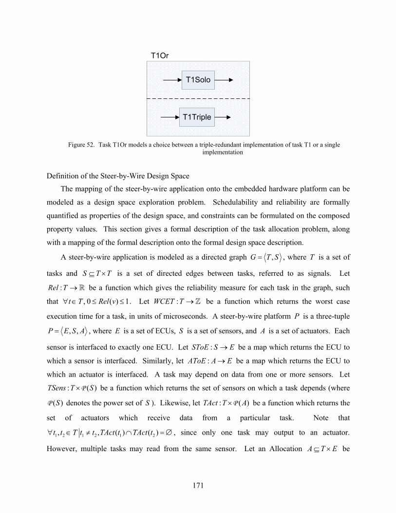
T1Solo
T1Triple
T1Or
Figure 52. Task T1Or models a choice between a triple-redundant implementation of task T1 or a single
implementation
Definition of the Steer-by-Wire Design Space
The mapping of the steer-by-wire application onto the embedded hardware platform can be
modeled as a design space exploration problem. Schedulability and reliability are formally
quantified as properties of the design space, and constraints can be formulated on the composed
property values. This section gives a formal description of the task allocation problem, along
with a mapping of the formal description onto the formal design space description.
A steer-by-wire application is modeled as a directed graph ,G T S= , where is a set of
tasks and is a set of directed edges between tasks, referred to as signals. Let
be a function which gives the reliability measure for each task in the graph, such
that . Let be a function which returns the worst case
execution time for a task, in units of microseconds. A steer-by-wire platform is a three-tuple
T
S T T⊆ ×
:Rel T →
, 0 ( ) 1t T Rel v∀ ∈ ≤ ≤ :WCET T →
P
, ,P E S A= , where is a set of ECUs, is a set of sensors, and is a set of actuators. Each
sensor is interfaced to exactly one ECU. Let be a map which returns the ECU to
which a sensor is interfaced. Similarly, let be a map which returns the ECU to
which an actuator is interfaced. A task may depend on data from one or more sensors. Let
be a function which returns the set of sensors on which a task depends (where
denotes the power set of ). Likewise, let
E S A
:SToE S E→
:AToE A E→
: (TSens T S×P )
)( )SP S : (TAct T A×P be a function which returns the
set of actuators which receive data from a particular task. Note that
1 2 1 2 1 2, , ( ) (t t T t t TAct t TAct t∀ ∈ ≠ ∩ =) ∅ , since only one task may output to an actuator.
However, multiple tasks may read from the same sensor. Let an Allocation be A T E⊆ ×
171

defined such that , t tt T p A p t e∀ ∈ ∃ ∈ = , for some ECU , and e
( ) ( )1 2 1 21 1 2 2 1 2, , , ,t t t tp t e p t e A t t implies p p∀ = = ∈ = = . There are several Allocations which
can be derived for a given application mapping onto a given platform. Let be the set of all
possible allocations. Note that
ASTAS E= . Constraints formally capture the requirements on the
application, and specify restrictions on composed property values. Let C be a set of constraints.
The allocation problem consists of finding a AS c C∈ ∀ ∈ , is satisfied over allocation . This
study focuses on two metrics which impact resource allocation, schedulability and reliability.
Requirements over both metrics are formulated as constraints. A schedulability constraint
imposes the requirement that for a given allocation, all ECUs meet the rate monotonic
scheduling utilization bound. A reliability constraint requires that an application meet some
minimum bound on composed reliability.
c a
The steer-by-wire specification is modeled as a design space using the AND-OR-LEAF tree
composition semantics. The composed application is modeled as an AND node in the AND-OR-
LEAF tree. The composed application consists of a set of tasks, each of which can potentially be
replicated. A task is either implemented singly (“single” redundancy) or with triple redundancy.
A triple-redundant case is modeled as an AND node containing three LEAF nodes. Each such
LEAF node is a copy or replica of the single case. Figure 53 illustrates the mapping of a task
into a set of AND-OR-LEAF tree nodes. All leaf nodes are assigned unique names, but each of
the four leaf nodes models the same task.
T1Triple
T1Or
T1Solo
= OR-Node
= AND-Node
= LEAF Node
Task T1
T1_1 T1_2 T1_3
Splitter Voter
Figure 53. Example mapping of a task T1 in the steer-by-wire specification into a set of AND-OR-LEAF tree
nodes
172

Properties are used to represent the quantitative aspects of the design space. All LEAF
nodes in the tree are assigned two non-composed properties: Resource and WCET. The WCET
property of a task is bound to the worst-case execution time of the task supplied in the task
model. The four LEAF nodes modeling each task in the application are all assigned the same
WCET value. Resource allocation is modeled as the binding of a value to the Resource variable
property. The domain of the Resource property represents the set of ECUs available in the
computation platform. All LEAF nodes’ Resource properties share the same domain, implying
that prior to the application of the constraints, any task can be mapped to any ECU in the
platform.
Reliability is modeled as a composable property. In the case of serial composition,
reliability composes multiplicatively. In the case of triple redundancy, reliability composes
according to equation (35). The AND-OR-LEAF tree semantics facilitate the representation of
composition with an AND node. AND composition is necessary to represent both serial
composition and parallel composition. Hence, the type of computation to employ for property
composition while exploring the space is not clear based simply on the type of tree node. It is
however discernable from the structure of the tree. Triple redundancy is modeled as an AND
node containing three LEAF nodes. At no other location in the tree does an AND node contain
LEAF nodes. Hence the property composition function for modeling reliability must examine
the structure of the tree in order to determine whether to apply multiplicative composition or the
redundant composition formula. The composition formula is also responsible for the
quantization of the probability values used to represent task reliability. The finite domain
constraint approach employed in DesertFD currently only supports integer-based mathematics,
so all floating point numbers are scaled by the constant 100. Rounding is implemented through
the addition of a scaled 0.5, followed by truncation implemented through integer division (ex. a
number x is rounded as follows: 50_100
xrnd x += , where the division operation is integer
division).
The PCL specification for reliability property composition is given in Figure 54. Lines (1)-
(3) define a helper function QMultVar which returns a quantized product of two variables.
Note that PCL only supports integer division. Line (6) defines the property function named
reliability. The function first determines which type of property composition to apply by
173

examining the structure of the tree from the context of application. The PCL function is applied
only at AND nodes in the tree, hence if all children of the context of application are LEAF
nodes, then it can be assumed that the node models a triple-redundancy. Whereas if it is not the
case that all children are leaf nodes, then the node models a serial reliability composition, and
simple multiplicative property composition is applied. Line (8) employs the isNodeLeaf
built-in function, which returns a Boolean true only if the context of invocation is a LEAF node
(or in the case of a list context, if all nodes in the list are LEAF nodes). The result is stored in
the isReplNode variable. Line (9) acquires the list of property variables corresponding to the
children of the application context, and Line (10) gets the first variable in the list. Since in the
replicated case, all replicated nodes are assumed to have the same reliability, the first property
value on the list is used in the composition. Line (11) assumes that the context of application
indicates a replicated composition, and implements equation (35), quantized as discussed above.
Line (14) assumes a non-replication context, and implements a simple product over all reliability
property variables of the children of the current context. Lines (15) and (16) multiply the result
of the context query with the respective replication results, and line (18) returns the sum of the
products. Since isReplNode is a 0/1 integer variable, the function returns either the value
calculated for ReplSum in line (15) or for NotReplSum in line (16).
174

(1) function var = QMultVar(var v1, var acc) (2) { (3) return(((v1 * acc) + 50)/100); (4) } (5) (6) property reliability( ) (7) { (8) var isReplNode = self().children().isNodeLeaf(); (9) list relPs = self().children().prop("reliability"); (10) var relVal = listHead(relPs); (11) var ReplRes = 3*((relVal*relVal+50)/100) (12) -(2*(relVal*relVal*relVal+5000)/10000); (13) (14) var NotReplRes = ForAllAcc(relPs, "QMultVar", 100); (15) var ReplSum = ReplRes *(isReplNode==1); (16) var NotReplSum = (isReplNode==0)*NotReplRes; (17) (18) return(ReplSum+NotReplSum); (19) }
Figure 54. PCL specification for reliability property composition
The representation of schedulability as a composable property in the design space definition
is challenging. The schedulability criterion dictates that for a given allocation, all tasks must
meet their deadlines. The determination of schedulability depends on an allocation, but the
allocation is the result of design space exploration. The difficulty of modeling schedulability lies
in the construction of the property composition rules and schedulability constraints so as to allow
constraint propagation to impact the set of potential allocations without needing to enumerate the
set. Schedulability in this study is determined by processor utilization. All tasks are assigned a
worst-case execution time, and all tasks are assigned the same period of 5 milliseconds.
Utilization, for a given allocation a AS∈ , is a function which is defined as
follows.
:autil E →
,
( ) ( )at T t e a
util e WCET t∈ < >∈
= ∑ (36)
Utilization is a composable property. However, it does not compose on the same decomposition
as reliability. Utilization composes along processor allocation boundaries. Hence, reification is
employed across all possible allocations in order to calculate the utilization of a processor. In the
design space model, each ECU is modeled as a member of a CustomDomain, modeling the
175

domain of the resource property for each task. Each such CustomDomain member is assigned
a property called utilization, whose composition is defined in the PCL specification given
in Figure 55. The property calculation employs in line (11) the built-in function allLeaves,
which returns as a list of variables all the leaves which descend from the context on which it is
invoked. The function spaceRoot returns the context corresponding to the root element of the
current DESERT Space, or in this case, the root element of the AND-OR-LEAF tree. Thus,
line (11) returns all the LEAF nodes in the AND-OR-LEAF tree. It then iterates across those
LEAF nodes in order to determine which have been allocated to the current context. The helper
function CalcUtil defined in line (1) is responsible for determining if a LEAF node has been
• allocated to the ECU modeled by the current context of invocation
• selected for inclusion in the current configuration.
If both of these criteria are met, then the WCET of the LEAF node is added to the utilization
total for the ECU. Line (3) determines if the LEAF task has been allocated to the current ECU,
by comparing the value of the resource property of the LEAF node against the ID of the current
context. The result is reified into the variable lMap. Line (5) multiplies the reified result of line
(3) with the value of the WCET property for the current LEAF node, and stores the result in the
variable lUtil (giving a value of 0 where the task has not been mapped to the current ECU, but
a value equal to the WCET when it has). Line (6) multiplies the WCET result by the value of the
select variable for the current LEAF, indicating that the WCET can only contribute to the
utilization bound when it has been selected for inclusion in the current configuration. The
resulting value is accumulated with the previous utilization for this ECU and returned.
176

(1) function var = CalcUtil(var leaf, var acc) (2) { (3) var lMap = (ToContext(leaf).prop("resource") == (4) self().getID()); (5) var lUtil = (lMap) * ToContext(leaf).prop("WCET"); (6) return acc + (lUtil * ToContext(leaf).sel()); (7) } (8) (9) property utilization ( ) (10) { (11) list leafList = spaceRoot().allLeaves(); (12) var util = ForAllAcc(leafList, "CalcUtil", 0); (13) return(util); (14) }
Figure 55. PCL specification for utilization calculation
Schedulability is modeled as a constraint over the utilization property of each ECU. For
each ECU in the model, the constraint in Figure 56 is added to the constraint set. The constraint
bound is derived from the shared 5 ms period between all tasks on each processor, and the 69.3%
upper bound on utilization.
constraint schedConstraint() { self.utilization() < 3465 }
Figure 56. Schedulability constraint, requiring that for each processor, the total compute time be bounded by 3465 microseconds
The property composition function implements the utilization calculation. However, the
calculation does not facilitate strong propagation, due to the use of reification to determine the
outcome of the calculation. As a result, the constraint applied to the utilization composition does
not result in significant pruning of the design space prior to distribution. Further, the steer-by-
wire application is not compute-bound. Distribution is employed more as a function of the
distribution of sensors throughout the platform rather than the need to split computation across
processing units to facilitate the meeting of real-time deadlines. However, with the replication
resulting from the analysis of reliability, the computation requirements of the application can
increase significantly. Hence, it is necessary to determine that the application does indeed meet
these minimum schedulability requirements.
177

The reason for the poor propagation performance of the utilization composition formula is
the circular dependence between resource allocation and the processor utilization constraint. In
order to facilitate early pruning of the design space, a second utilization constraint is formulated
which breaks this circular dependence. It can be noted that if the total computational
requirements across all tasks of an application exceeds the total available computation time on all
resources, then the configuration cannot be implemented on the platform. The total computation
time required by an application can be calculated by summing the worst-case execution times of
all selected tasks in the design space. The total available computation time can be calculated by
multiplying the number of ECUs in the platform by the period of computation which is shared
across all tasks. This is represented in the design space using additive property composition over
a property called computeTime. LEAF nodes in the tree are assigned the worst-case execution
time of the WCET property. A constraint is placed at the root node of the AND-OR-LEAF tree
which limits the total composed computeTime property to the upper bound of available
compute time. Figure 57 gives the OCL specification of the total compute time constraint. The
right-hand side of the equation represents the upper bound on the total compute time available in
the network, assuming that all tasks execute at a 5 ms rate. There are five processors in the
network, and each must meet the 69.3% utilization bound, giving 5 times (5000*0.693)
microseconds of total available compute time. The constraint is not a tight constraint, due to the
significant slack in the schedule of the processors. However, the constraint does eliminate those
configurations which are grossly unschedulable, prior to the determination of an allocation.
constraint compTime() } self.computeTime() < 5*5*693 }
Figure 57. Constraint on total computation time for a five-processor configuration, with a five millisecond period
Resource allocation constraints are employed in the design space model to represent rules of
composition and allocation. It was noted above that equation (35) improves reliability only
when the reliability of the task to be replicated is greater than 0.5. A constraint is placed in the
design space model at each of the OR nodes modeling the potential for replication, stating that if
the task’s reliability is less than 0.5, then the singleton alternative should be automatically
178

selected. While the constraint solver can implicitly derive this result through property
composition, the addition of the constraint speeds the propagation. Figure 58 gives an OCL
implementation of this selection constraint, as applied to the example AND-OR-LEAF tree given
in Figure 53.
constraint selConstr() { (self.children(“T1Solo”).reliability() < 50) implies (self.implementedBy()=self.children(“T1Solo”)) }
Figure 58. Selection constraint applying to the OR node T1Or in Figure 53, stating that if the reliability of the modeled task is less than 50, then do not replicate the task
The reliability property composition function assumes that the failure of a component or task
is an independent event from the failure of other tasks. Given that many tasks fail due to
hardware faults, this assumption is not necessarily valid. However, in an attempt to separate the
failure modes of the replicated tasks, constraints are inserted into the model at each AND node
modeling task replication, stating that all replicated tasks must be allocated to different
resources. A more valid assumption is that the failure modes of tasks allocated to separate
resources are not as related as those of co-located tasks. Three constraints are inserted at each
AND node modeling replication, stating that the resources of each of the replicated nodes cannot
be equal. The constraint corresponding to the T1Triple node in Figure 53 is given in Figure
59.
179

constraint replConstr1() { self.children(“T1_1”).resource() <> self.children(“T1_2”).resource() } constraint replConstr2() { self.children(“T1_1”).resource() <> self.children(“T1_3”).resource() } constraint replConstr3() { self.children(“T1_2”).resource() <> self.children(“T1_3”).resource() }
Figure 59. Replication constraints requiring that no replicated nodes share a resource
It was noted in the platform discussion that each sensor and each actuator is interfaced to
exactly one ECU. While sensor information can be relayed from ECU to ECU, it leads to a more
efficient, lower-latency implementation when tasks which directly depend on sensor information
can be allocated to the ECU which is interfaced to the sensor. Likewise, for tasks which output
to actuators, ideally those tasks are allocated to the resource which interfaces to the actuator. It
may not be possible to create an allocation where all such constraints are met. For example,
some tasks read the wheel position information from all four wheel sensors. The design space
model employs constraint utilization to model the desire that tasks be mapped to resources which
interface to the appropriate sensors and actuators. The constraint solver attempts to maximize
total constraint utilization. For those situations where all such co-location constraints cannot be
met, an allocation is produced which attempts to meet most of the constraints. Recall that
is a map which returns the set of sensors which directly interface to a task.
Similarly, is a map which returns the set of actuators to which a task interfaces.
Then, , ideally the following constraints hold:
: (TSens T S×P )
): (TAct T S×P
,t T a AS∀ ∈ ∀ ∈
( ), , ( )
( ), , ( )
s TSens t t SToE s a
c TAct t t AToE c a
∀ ∈ ∈
∀ ∈ ∈ (37)
The constraints are extended to cover the replicated tasks as well. Obviously, for the replicated
tasks, the requirement that states that replicated tasks cannot be co-located, and the reified
constraint stating that tasks should be located on the resource which interfaces to their dependent
180

sensors and actuators are directly in conflict. Due to the optimization of constraint utilization,
the constraint solver attempts to satisfy the constraints in equation (37) only where possible.
Each such allocation constraint is assigned a utilization value of 10 (owning to the fact that no
allocation constraint has priority over any other allocation constraint).
The final constraint that is added to the design space specification is a constraint on the
composed reliability of the system. Figure 60 gives the OCL implementation of the reliability
constraint, which is assigned to the root node of the AND-OR-LEAF tree as its context of
application. The constraint requires that the composed system be greater than 50. This appears
to be a weak requirement, but due to the multiplicative composition exhibited by reliability,
highly reliable configurations are difficult to achieve.
constraint reliabilityConstr() { self.reliability() > 50 }
Figure 60. Constraint on the composed reliability of the system, applied at the root context
This case study seeks to model reliability as a composable property, used in the context of
pruning the resource allocation space of embedded automotive software. It does not pretend to
be a study in modeling component reliability. Due to the lack of quality reliability estimates for
the tasks in the application model, a random reliability value was assigned to each task, by
sampling a random variable uniformly distributed on the interval [85, 99]. If proper reliability
metrics can be obtained for the tasks in the system, the analysis approach can still be applied.
Exploration Results
The design space model discussed above, together with the constraint set was explored using
DesertFD. All constraints were parsed and translated and applied in the finite domain constraint
environment. The space initially contains configurations. The exploration of the space
revealed several details about the structure of the design space. The space was determined to be
highly under-constrained. There are a very large number of potential solutions which satisfy all
imperative constraints. It was described in previous chapters that the exploration of a large,
under-constrained space leads to exponential growth in the memory requirements of the search.
An interesting aspect of this particular design space is the fact that all solutions to the space seem
6610
181
to exhibit the same maximum constraint utilization value of 550. The best-case utilization search
encounters a single solution with utilization of 550 and proceeds to search for a solution which
exhibits better utilization. This subsequent search neither encounters any solutions to the space
which better this utilization value, nor is able to terminate the search, due to the size of the space
and the dependence of the search on distribution. The successful solution was encountered in a
depth-first search, requiring 131 distribution steps. The single encountered solution presents a
composed reliability of 51, and utilization values on each processor between 3457 and 3054. Of
the 19 tasks in the application, the solution selects 14 for triple-redundant implementation, in
order to satisfy the reliability constraint. Five tasks are implemented without replication in order
to satisfy schedulability requirements. The time required to encounter this single solution was
about 0.5 seconds.
Conclusions and Future Analyses
The design space presented in this case study is under-constrained. The constraints on
reliability facilitate pruning of the space. Schedulability constraints on processor utilization can
only impact the search after an allocation of tasks to processors has been determined, thus only
facilitating pruning after significant distribution. The slack in the schedule implies that many
configurations are schedulable according to rate monotonic criteria. In order to achieve a better
pruning of the space, the space must be analyzed along other axes. Specifically, distribution of
tasks imposes delays in the end-to-end latency of computation. The schedulability analysis does
not take into account the dependencies between tasks, and ignores the issue of scheduling
communications over the fault-tolerant bus. Addressing these and other issues can lead to a
significant contraction of the design space.
182

REFERENCES
[1] Oliphant, M. W., "Radio Interfaces Make the Difference in 3G Cellular Systems," IEEE Spectrum, vol. 37, pp. 53-58, 2000.
[2] Perry, T. S., "Consumer electronics," IEEE Spectrum, vol. 37, pp. 51-56, 2000. [3] Jones, W. D., "Building Safer Cars," IEEE Spectrum, vol. 39, pp. 82-85, 2002. [4] Snoonian, D., "Smart Buildings," IEEE Spectrum, vol. 40, pp. 18-23, 2003. [5] Lea, R., Gibbs, S., Dara-Abrams, A., and Eytchison, E., "Networking Home
Entertainment Devices with HAVi," IEEE Computer, vol. 33, pp. 35-43, 2000. [6] Verkest, D., "Machine Chameleon," IEEE Spectrum, vol. 40, pp. 41-46, 2003. [7] Bretz, E. A., "By-Wire Cars Turn the Corner," IEEE Spectrum, vol. 38, pp. 68-73, 2001. [8] Cass, S., "2001: A Mars Odyssey," IEEE Spectrum, vol. 38, pp. 58-65, 2001. [9] DiGregorio, B. E., "Mars: Dead or Alive?," IEEE Spectrum, vol. 40, pp. 36-41, 2003. [10] Ait-Ameur, Y., Bel, G., Boniol, F., Pairault, S., and Wiels, V., "Robustness Analysis of
Avionics Embedded Systems," LCTES, San Diego, CA, USA, 2003. [11] Scott, P., "Aerospace & Military," IEEE Spectrum, vol. 37, pp. 97-102, 2000. [12] Napper, S., "Embedded System Design Plays Catch-up," IEEE Computer, vol. 31, pp.
120-119, 1998. [13] Peterson, I., Fatal Defect: Chasing Killer Computer Bugs. New York: Random House,
1995. [14] Wilner, D., "Vx-Files: What Really Happened on Mars?," in Keynote Address, RTSS,
1997: http://research.microsoft.com/research/os/mbj/Mars_Pathfinder/Mars_Pathfinder.html (As related by Mike Jones), 1997.
[15] Oberg, J., "Why the Mars Probe," IEEE Spectrum, vol. 36, pp. 34-39, 1999. [16] Jezequel, J.-M. and Meyer, B., "Design by Contract: The Lessons of Ariane," IEEE
Computer, vol. 30, pp. 129-130, 1997. [17] Sztipanovits, J. and Karsai, G., "Embedded Software: Challenges and Opportunities,"
Emsoft, 2001.
183

[18] available at: http://e-www.motorola.com/webapp/sps/site/homepage.jsp?nodeId=03C1TR0467
[19] available at: http://www.xilinx.com/xlnx/xil_prodcat_landingpage.jsp?title=Virtex-
II+Pro+FPGAs [20] Richards, M., Campbell, D., Cottel, D., and Judd, R., "Introduction to Morphware:
Software Architecture for Polymorphous Computing Architectures," Georgia Institute of Technology, SPAWAR, February 23, 2004.
[21] Liu, C. and Layland, J., "Scheduling Algorithms for Multiprogramming in a Hard-Real-
Time Environment," Journal of the ACM, vol. 20, pp. 46-61, 1973. [22] Dantzig, G., "Programming in a Linear Structure," Comptroller, Washington, DC,
February, 1948. [23] Dantzig, G., Linear Programming and Extensions. Princeton, New Jersey: Princeton
University Press, 1963. [24] Chvatal, V., Linear Programming: W. H. Freeman, 1983. [25] Schrijver, A., Theory of Linear and Integer Programming: John Wiley & Sons Ltd, 1986. [26] Aho, A., Hopcroft, J., and Ullman, J., Data Structures and Algorithms: Addison-Wesley
Pub Co., 1983. [27] Balas, E., Ceria, S., and Cornuejols, G., "Mixed 0-1 Programming by Lift-and-Project in
a Branch-and-Cut Framework," Management Science, vol. 42, pp. 1229-1246, 1996. [28] Padberg, M. and Rinaldi, G., "A Branch and Cut Algorithm for a Symmetric Travelling
Salesman Polytope," SIAM Review, vol. 33, pp. 60-100, 1991. [29] Barnhart, C., Johnson, E., Nemhauser, G., and Savelsberg, P., "Branch and Price:
Column Generation for Huge Integer Programs," Operations Research, vol. 46, pp. 316-329, 1998.
[30] available at: http://www.ilog.com [31] available at: http://www.lindo.com [32] available at: http://www-306.ibm.com/software/data/bi/osl [33] Prakash, S. and Parker, A., "Synthesis of application-specific multiprocessor
architectures," DAC, San Francisco, CA, USA, June, 1991.
184

[34] Kaul, M. and Vemuri, R., "Design-space exploration for block-processing based temporal partitioning of run-time reconfigurable systems," Journal of Vlsi Signal Processing Systems for Signal Image and Video Technology, vol. 24, pp. 181-209, 2000.
[35] Bockmayr, A., "Logic programming with pseudo-Boolean constraints," in Constraint
Logic Programming, Selected Research, F. Benhamou and A. Colmerauer, Eds.: MIT Press, 1993, pp. 327-350.
[36] Davis, M., Logemann, G., and Loveland, D., "A Machine Program for Theorem
Proving," Communications of the ACM, vol. 5, pp. 394-397, 1962. [37] Moskewicz, C., Madigan, C., Zhao, Y., Zhang, L., and Malik, S., "Chaff: Engineering an
Efficient SAT Solver," Design Automation Conference, 2001. [38] Aloul, F., Ramani, A., Markov, I., and Sakallah, K., "PBS: A Backtrack-Search Pseudo-
Boolean Solver and Optimizer," Fifth International Symposium on Theory and Application of Satisfiability Testing, Cincinnati, Ohio, May 6-9, 2000.
[39] Bockmayr, A. and Kasper, T., "Pseudo-Boolean and Finite Domain Constraint
Programming: A Case Study," in Deklarative Constraint Programmierung, U. Geske and H. Simonis, Eds. Dresden, 1996.
[40] Jaffar, J. and Maher, M. J., "Constraint Logic Programming - a Survey," Journal of Logic
Programming, vol. 20, pp. 503-581, 1994. [41] Marriott, K. and Stukey, P., Programming with Constraints. Cambridge, MA: MIT Press,
1998. [42] Schild, K. and Wurtz, J., "Off-Line Scheduling of a Real-Time System," ACM
Symposium on Applied Computing, Proceedings of, Atlanta, GA, 1998. [43] Henz, M. and Wurtz, J., "Constraint-based time-tabling - A case study," Applied Artificial
Intelligence, vol. 10, pp. 439-453, 1996. [44] available at: http://www.friartuck.net/news/2002/Media-NBS.htm [45] Van Hentenryck, P., Constraint Satisfaction in Logic Programming: MIT Press, 1989. [46] available at: http://www.mozart-oz.org [47] Kuchcinski, K., "Constraints-driven scheduling and resource assignment," ACM
Transactions on Design Automation of Electronic Systems, vol. 8, pp. 355-383, 2003. [48] Dincbas, M., Vanhentenryck, P., Simonis, H., Aggoun, A., and Herold, A., "The Chip
System - Constraint Handling in Prolog," Lecture Notes in Computer Science, vol. 310, pp. 774-775, 1988.
185

[49] Jaffar, J., Michaylov, S., Stuckey, P. J., and Yap, R. H. C., "The Clp(R) Language and
System," ACM Transactions on Programming Languages and Systems, vol. 14, pp. 339-395, 1992.
[50] Smolka, G., "The Oz programming model," Computer Science Today, vol. 1000, pp. 324-
343, 1995. [51] Wurtz, J., "Oz Scheduler: A Workbench for Scheduling Problems," IEEE International
Conference on Tools with Artificial Intelligence, Toulouse, France, November 16-19, 1996, 1996.
[52] Eles, P., Kuchcinski, K., and Peng, Z. B., "Embedded System Synthesis by Timing
Constraints Solving," ISSS, Antwerp, Belgium, Sept 17-19, 1997. [53] Kuchcinski, K., "Constraints-driven design space exploration for distributed embedded
systems," Journal of Systems Architecture, vol. 47, pp. 241-261, 2001. [54] Harvey, W. D. and Ginsberg, M. L., "Limited Discrepency Search," Fourteenth
International Joint Conference of Artificial Intelligence (IJCAI-95), 1995. [55] Beldiceanu, N., Bourreau, E., Simonis, H., and Chan, P., "Partial search strategy in
CHIP," Second Metaheuristic International Conference, Sophia Antipolis, France, July 21-24, 1997.
[56] Kuchcinski, K., "Synthesis of Distributed Embedded Systems," Euromicro Workshop on
Digital System Design, Milan, Italy, Sept 8-10, 1999. [57] Szymanek, R. and Kuchcinski, K., "Partial Task Assignment of Task Graphs under
Heterogeneous Resource Constraints," Design Automation Conference (DAC), Anaheim, CA, USA, June, 2003.
[58] Szymanek, R. and Kuchcinski, K., "A Constructive Algorithm for Memory-Aware Task
Assignment and Scheduling," Ninth International Symposium on Hardware/Software Codesign, Copenhagen, Denmark, 2001.
[59] Kirkpatrick, S., Gelatt, C., and Vecchi, M., "Optimization by Simulated Annealing,"
Science, vol. 220, pp. 671-680, 1983. [60] Bazargan, K., Kastner, R., and Sarrafzadeh, M., "3-D Floorplanning: Simulated
Annealing and Greedy Placement Methods for Reconfigurable Computing Systems," Design Automation for Embedded Systems, vol. 5, pp. 329-338, 2000.
[61] Ernst, R., Henkel, J., and Benner, T., "Hardware-software Cosynthesis for
microcontrollers," IEEE Design & Test of Computers, pp. 64-75, 1993.
186

[62] Spears, W., De Jong, K., Back, T., Fogel, D., and de Garis, H., "An Overview of Evolutionary Computation," European Conference on Machine Learning, Proceedings of, vol. 667, pp. 442-459, 1993.
[63] "The Hitch-Hiker's Guide to Evolutionary Computation: A list of Frequently Asked
Questions (FAQ)" available at: ftp://rtfm.mit.edu/pub/usenet/news,answers/ai-faq/genentic
[64] Fonseca, C. and Fleming, P., "An Overview of Evolutionary Algorithms in
Multiobjective Optimization," Evolutionary Computation, vol. 3, pp. 1-16, 1995. [65] Palesi, M. and Givargis, T., "Multi-Objective design space exploration using genetic
algorithms," CODES, Estes Park, Colorado, USA, 2002. [66] Steuer, R., Multiple Criteria Optimization: Theory, Computation and Application. New
York: Wiley, 1986. [67] Blickle, T., Teich, J., and Thiele, L., "System-Level Synthesis Using Evolutionary
Algorithms," Design Automation for Embedded Systems, vol. 3, pp. 23-58, 1998. [68] Axelsson, J., "Hardware/software partitioning aiming at fulfilment of real-time
constraints," Journal of Systems Architecture, vol. 42, pp. 449-464, 1996. [69] Wang, S., Merrick, J., and Shin, K., "Component Allocation with Multiple Resource
Constraints for Large Embedded Real-Time Software Design," RTAS, 2004. [70] Givargis, T. and Vahid, F., "Parameterized System Design," CODES, San Diego, CA,
USA, 2000. [71] Pareto, V., "Cours d'economic politique," Rouge, Laussanne, Switzerland, 1896. [72] Givargis, T. and Vahid, F., "Platune: A tuning framework for system-on-a-chip
platforms," IEEE Transactions on Computer-Aided Design of Integrated Circuits and Systems, vol. 21, pp. 1317-1327, 2002.
[73] Givargis, T., Vahid, F., and Henkel, J., "System-level exploration for Pareto-optimal
configurations in parameterized system-on-a-chip (December 2002)," IEEE Transactions on Very Large Scale Integration (Vlsi) Systems, vol. 10, pp. 416-422, 2002.
[74] Vahid, F. and Givargis, T., "Platform tuning for embedded systems design," Computer,
vol. 34, pp. 112-114, 2001. [75] Givargis, T., Vahid, F., and Henkel, J., "Evaluating Power Consumption of
Parameterized Cache and Bus Architectures in System-on-a-Chip Designs," IEEE Transactions on Very Large Scale Integration (VLSI) Systems, vol. 9, pp. 500-508, 2001.
187

[76] Thomas, D. E., Adams, J. K., and Schmit, H., "A Model and methodology for Hardware-software codesign," IEEE Design & Test of Computers, pp. 6-11, 1993.
[77] Kathail, V., Aditya, S., Schreiber, R., Rau, B. R., Cronquist, D. C., and Sivaraman, M.,
"PICO: Automatically Designing Custom Computers," IEEE Computer, pp. 39-47, 2002. [78] Snider, G., "Spacewalker: Automated Design Space Exploration for Embedded Computer
Systems," HP Labs Palo Alto HPL-2001-220, September 10, 2001. [79] Neema, S., "System-Level Synthesis of Adaptive Computing Systems," Ph.D.
Dissertation. Vanderbilt University, 2001. [80] Neema, S., Sztipanovits, J., Karsai, G., and Butts, K., "Constraint-based design-space
exploration and model synthesis," Embedded Software, Proceedings, vol. 2855, pp. 290-305, 2003.
[81] "Object Constraint Language Specification, Version 1.1," Object Management Group,
September, 1997. [82] Bryant, R., "Graph-Based Algorithms for Boolean Function Manipulation," IEEE
Trasactions on Computers, vol. C-35, pp. 677-691, 1986. [83] Ledeczi, A., Bakay, A., Maroti, M., Volgyesi, P., Nordstrom, G., Sprinkle, J., and Karsai,
G., "Composing domain-specific design environments," Computer, vol. 34, pp. 44-+, 2001.
[84] Karsai, G., Sztipanovits, J., Ledeczi, A., and Bapty, T., "Model-integrated development
of embedded software," Proceedings of the Ieee, vol. 91, pp. 145-164, 2003. [85] Nordstrom, S., Shetty, S., Chhokra, K. G., Sprinkle, J., Eames, B., and Ledeczi, A.,
"ANEMIC: Automatic interface enabler for model integrated computing," Generative Programming and Component Engineering, Proceedings, vol. 2830, pp. 138-150, 2003.
[86] Becker, P. W. and Jensen, F., Design of Systems and Circuits for Maximum Reliability or
Maximum Production Yield. Tokyo, Japan: McGraw-Hill, 1977.
188