978-1-4577-0351-5/11/$26.00 c©2011 IEEE

Exploiting Temporal Complex Network Metrics in Mobile Malware Containment

John TangComputer Laboratory

University of Cambridgejkt27@cam.ac.uk

Cecilia MascoloComputer Laboratory

University of Cambridgecm542@cam.ac.uk

Mirco MusolesiSchool of Computer Science

University of St. Andrewsmirco@cs.st-andrews.ac.uk

Vito LatoraDipartimento di FisicaUniversity of Catania

latora@ct.infn.it

Abstract—Malicious mobile phone worms spread betweendevices via short-range Bluetooth contacts, similar to the prop-agation of human and other biological viruses. Recent workhas employed models from epidemiology and complex networksto analyse the spread of malware and the effect of patchingspecific nodes. These approaches have adopted a static viewof the mobile networks, i.e., by aggregating all the edges thatappear over time, which leads to an approximate representationof the real interactions: instead, these networks are inherentlydynamic and the edge appearance and disappearance arehighly influenced by the ordering of the human contacts,something which is not captured at all by existing complexnetwork measures.

In this paper we first study how the blocking of mal-ware propagation through immunisation of key nodes (evenif carefully chosen through static or temporal betweennesscentrality metrics) is ineffective: this is due to the richnessof alternative paths in these networks. Then we introduce atime-aware containment strategy that spreads a patch messagestarting from nodes with high temporal closeness centrality andshow its effectiveness using three real-world datasets. Temporalcloseness allows the identification of nodes able to reach mostnodes quickly: we show that this scheme reduces the cellularnetwork resource consumption and associated costs, achieving,at the same time, complete containment of malware in a limitedamount of time.

Keywords-Mobile Malware; Temporal Graphs; TemporalCentrality.

I. INTRODUCTION

Smartphones are not only ubiquitous, but also an essentialpart of life for many people who carry such devices throughtheir daily routine. It comes at no surprise then that recentstudies have shown that the mobility of such devices mimicthat of their owners’ schedule [8], [23]. This fact constitutesan opportunity for devising efficient protocols and appli-cations, but it also represents an increasing security risk:as with biological viruses that can spread from person toperson, mobile phone viruses can also leverage the samesocial contact patterns to propagate via short-range wirelessradio such as Bluetooth and WiFi. For example, when secu-rity researchers downloaded Cabir [1] – a proof-of-conceptmobile worm – for analysis, they discovered the full risk asit broke loose, replicating from the test device to externalmobile phones. This prompted the need for specially radioshielded rooms to securely test such malicious code [13].

Until recently though, mobile malware has been devel-oped only for proof-of-concept experiments with very lim-

ited and non malicious effects on users [20], [18]. However,the immense popularity and improvements in smartphonetechnology have attracted the attention of a growing numberof attackers. In particular, increasing economic incentiveshave been the motivation of more recent exploits, for ex-ample stealing private data such as phone contacts [2];transferring call credit to other accounts [3]; and traditionalexploits such as premium rate number dialling [4].

Unlike desktop computers mobile malware can spreadthrough both short-range radio (i.e., Bluetooth and WiFi)and long-range communication (i.e., SMS, MMS andemail) [14]. Long-range malicious traffic can potentiallybe contained by the network operator by scanning everymessage against a database of known malware [17], how-ever, short-range propagation might fall under the radar ofcentralised service providers: effective schemes to defendagainst short-range mobile malware spreading are necessary.Also, while a global patching of the devices through cellularconnectivity is the natural solution and is in theory possible,in practice, there are potential constraints with respect to thecellular network capacity and server bandwidth [9].

Being highly correlated with human contacts, understand-ing how such malware propagates requires an accurateanalysis of the underlying time-varying network of contactsamongst individuals. State-of-the-art solutions on mobilemalware containment have ignored two important temporalproperties: firstly, the time order, frequency and duration ofcontacts; and secondly, the time of day a malicious messagestarts to spread and the delay of a patch [26], [27]. Instead,we argue that the temporal dimension is of key importancein devising effective solutions to this problem.

With this in mind, the focus of this study is to investigatethe effectiveness of two containment strategies based on tar-getting key nodes, taking into account these temporal charac-teristics. We firstly investigate a traditional strategy, inspiredby studies on error and attack tolerance of networks [5],exploiting a static and a time-aware enhanced version ofbetweenness centrality which provide the best measure ofnodes that mediate or bridge the most communication flows.According to this strategy the nodes that act as mediators arepatched to block the path of a malicious message. However,due to temporal clustering and alternative temporal paths,in most cases, such strategies merely slow the malware and

does not stop it. In other words, a scheme based solely onimmunisation of key nodes is not sufficient, instead quickspreading of the patch is necessary for most networks. Wepropose a solution based on local spreading of patchesthrough Bluetooth, i.e., exploiting the same mechanism usedby the malware itself. The key issue in this approach isto select the right nodes as starting points of the patchingprocess. Temporal betweenness only provides a quantitativemeasure of the number of communication paths over timethat go through a certain node and it proves to be sub-optimalmetric for this. A metric capable of identifying nodes thatcan reach a large quantity of other nodes quickly is needed.Our choice fell on temporal closeness centrality which ranksnodes by the speed at which they can disseminate a messageto all other nodes in the network. We show that this strategycan reduce the cellular network resource consumption andassociated costs, achieving at the same time a completecontainment of the malware in a limited amount of time.

In the following sections, we will first introduce somepreliminary definitions related to temporal graph analysisand metrics and then present a detailed study of our proposedcontainment scheme using real-world traces.

II. TEMPORAL NETWORKS

Temporal graphs have recently been proposed [21], [11]to study real dynamic datasets, with the intuition that thebehaviour of dynamic networks can be more accuratelycaptured by a sequence of snapshots of the network topologyas it changes over time instead of using a representationwhereby all the contacts are aggregated into a single staticgraph. From this, temporal versions of shortest path [21]have demonstrated that, since static analysis ignores timeordering of contacts, static shortest paths overestimate theavailable links and underestimate the actual shortest pathlength.

We now provide a brief overview of these conceptsin relation to the problem of designing effective malwarecontainment schemes. Since Bluetooth radio can only handleuni-directional transmissions (from the scanning device tothe scanned device) we define a directed temporal graphwhich can be thought of as an ordered sequence of directedgraphs1. A state of the network topology is calculatedby aggregating all the directed edges that appear insidea certain time window. An example, using a dataset ofcontacts among students and staff at Cambridge, is givenin Figure 1 (more details about the dataset are provided inSection IV-A)2: Figure 1(a) shows a temporal graph witha sequence of six graphs, each of them representing thecontacts among devices in a time window of 24-hours. Thecorresponding aggregated static graph (which reports all thelinks amongst nodes, without any information about time) is

1This does not lose generality of bi-directional communication sincetransmissions can still be reciprocated during the same encounter.

2Direction of edges have been removed for clarity.

1

2

3

456

7

8

9

10

11

12

1314 15

16

17

18

Thu

1

2

3

456

7

8

9

10

11

12

1314 15

16

17

18

Fri

1

2

3

456

7

8

9

10

11

12

1314 15

16

17

18

Sat

1

2

3

456

7

8

9

10

11

12

1314 15

16

17

18

Sun

1

2

3

456

7

8

9

10

11

12

1314 15

16

17

18

Mon

1

2

3

456

7

8

9

10

11

12

1314 15

16

17

18

Tue

(a) Temporal Graph

1

2

34

567

8

9

10

11

1213

14 1516

17

18

Static

(b) Static Graph

Figure 1. (a) Temporal Graph showing contacts using 24-hour windowsand (b) aggregated static graph for the CAMBRIDGE dataset. Nodesrepresent devices; two nodes are linked if there was a Bluetooth contactwithin that 24-hour window.

shown in Figure 1(b). The static graph misses the circadianrhythms that can instead be observed in the temporal graph.Also note that the high density of links within the staticgraph, which we will see later, contributes to problems indiscriminating between important nodes for the calculationof static centrality; instead a temporal graph is requiredto capture the rich temporal information of the interactionpatterns.

To give an intuition as to why temporal graphs andtemporal paths are necessary, consider the temporal graphand associated aggregated static graph in Figure 2. If weconsider a shortest path from node A to F , according tothe static graph there is a 2-hop path (A,C, F ), when infact taking into account the time ordering of contacts inthe temporal graph, we see that such a path does not existin reality; instead, the actual shortest path is of 3-hops(A,C,E, F ).

More formally, given a real-world contact trace startingat tmin and ending at tmax, the directed temporal graphGw(tmin, tmax) is defined as the ordered sequence of graphs(G0, G2, . . . , GT−1) where T = ((tmax − tmin)/w) =|Gw(tmin, tmax)| is the number of graphs in the sequenceand w is the size of each time window expressed in sometime units (e.g., seconds or hours). There exists a directedlink from i to j in GT if there is a contact from i to j duringthe time interval [(tmin+(w×T )), (tmin+(w×(T +1)))).All graphs in the temporal graph have the same set of nodesV .

From this a temporal path starting at i and finishing atj can be defined over Gw(tmin, tmax) as a sequence of khops via a distinct node nWk

k at time window Wk:

phij = (nW01 , . . . , nWk

k ) (1)

where i = n1, j = nk, node nk is passed a message attime window Wk ≥ Wk−1, 0 ≤ Wk < T and h is themaximum hops through which a message is replicated withinthe same window. Subsequent definitions implicitly set h =1, since higher values of h lead to similar performance ofthe containment schemes. We call Qij the set of all temporalpaths between nodes i and j. If a temporal path from i to j

A

C

E F

B

D

A

C

E F

B

D

A

C

E F

B

D

A

C

E F

B

D

t1 t2 t3 t4 time

A

C

E F

B

D

t5

A

C

E F

B

D

t6

A

C

E F

B

D

Figure 2. Example directed Temporal Graph (top) and aggregated staticgraph (bottom).

does not exist i.e. Qij = ∅, we say that (i, j) is a temporallydisconnected node pair, and we set the distance dij =∞.

Using the function D(pij) = (w×Wk) which returns thereal delivery time (at window Wk) for the given path relativeto tmin, the shortest temporal path length is defined as:

dij = min(D(qij)),∀qij ∈ Qij (2)

From this we define the set Sij of shortest temporal pathsbetween i, j as:

Sij = {pij ∈ Qij | D(pij) = dij} (3)

We define the temporal efficiency Eij between nodes iand j for the time interval tmin to tmax as:

Eij(tmin, tmax) =1

dij(tmin, tmax) + 1(4)

We can then define the average temporal efficiency E as:

E(tmin, tmax) =1

N(N − 1)

∑i,j∈Vi 6=j

Eij(tmin, tmax) (5)

For brevity we shall also refer to this as efficiency. Efficiencynaturally handles disconnected node pairs since it gives usthe harmonic mean of delays between all node pairs.

III. TEMPORAL CENTRALITY METRICS FOR MALWARECONTAINMENT

Let us consider a simple scenario where a person receivesa malicious message on their device in the early hours ofthe morning and the malicious program replicates itself toany devices it meets during the day, for example at workand while socialising in the evening.

A simple strategy consists of immunising only the nodeswhich mediate the most communication flows. Betweennesscentrality metrics have been devised for static complexnetwork graphs to measure this quantity [24] and we haveextended this measure to incorporate the temporal dimen-sion [22]. However, we will show that no matter how wechoose these nodes (e.g., by using a static or temporal met-rics to find these path mediators), this strategy is ineffective.The intuition behind this is given through the example inFigure 2. Consider the shortest temporal paths from node Ato node F , namely (A,C,E, F ) and a longer (both in terms

A E

t1 t2

C

t3 t4 t5

B D E

t6

F

start

F

(a)

A C

t1 t2

F

t3

B D

start

E

t4

(b)Figure 3. (a) Two temporal paths from node A to node F . (b) Temporalminimum spanning tree with source node A showing shortest temporalpaths to all other nodes.

of hops and time of delivery) temporal path (A,B,D,E, F ),also illustrated in Figure 3(a). If we consider the simple caseof patching a single node in an attempt to block the malwarefrom spreading, the best choice would be node C, as theone on most temporal paths, however notice that node Bprovides an alternative path to F albeit a longer path.

Our second strategy relies on the ability to spread a patchmessage quickly throughout the network; we utilise close-ness centrality which is able to capture this property. Wenow formally describe these temporal centrality measures.

A. Temporal Betweenness CentralityThe static betweenness centrality of a node i is defined

as the fraction of shortest paths between all pairs of nodeswhich pass through i [24]. Betweenness is commonly usedto discover nodes which are critical for information flowand, therefore, prioritised for patching. Hence, to capturethe notion of temporal betweenness it is important to takeinto account not only the number of shortest paths whichpass through a node, but also the length of time for whicha node along the shortest path retains a malicious mes-sage before forwarding it to the next node. For example,consider the 2-hop shortest temporal path from node Ato D, (A,B,D). In terms of time, this path could berepresented as (A,B,B,B,D) since the malicious messageresides on node B for 3 time windows, and so we want toassign a higher value as patching this node will lead to ahigher probability of stopping the malicious message fromspreading. From this, for a given time window T we definethe temporal betweenness centrality of node i as:

Bi(T ) =1

(N − 1)(N − 2)

∑j∈Vj 6=i

∑k∈Vk 6=ik 6=j

U(i, T, j, k)

|σj,k(i)|(6)

where the function U returns the number of shortest tempo-ral paths from j to k in which node i has either received amessage at time window T or is holding a message from apast time window until the next node is met at some timeT ′ > T and σj,k(i) ⊆ Sjk is the set of shortest temporalpaths from node i to j which pass through node i, definedwhen σj,k(i) 6= ∅. In the case when σj,k(i) = ∅, i.e., node iis totally isolated, we set its betweenness to zero. Finally, theaverage temporal betweenness value across all time windowsfor each node i is:

Bi =1

T

T−1∑t=0

Bi(t). (7)

CAMBRIDGE INFOCOM MITN 18 78 100

Start Date 3 Feb 2010 23 Apr 2006 26 Jul 2004Duration 10 Days 5 days 280 days

Scanning Rate 30 sec 2 min 5 min

Table IEXPERIMENTAL DATASETS

B. Temporal Closeness Centrality

Two nodes of a static graph are said to be close to eachother if their geodesic distance is small. In a static graph anestimation of the global closeness of a node i is obtainedas the average static shortest path length to all other nodesin the graph [24]. Similarly, we can extend the definitionof closeness to temporal graphs using the temporal shortestpath length between nodes, which is a measure of how fast asource node can deliver a message to all the other nodes ofthe network. This can be thought of as a temporal minimumspanning tree (see Figure 3(b)). Given the shortest temporaldistance dij(tmin, tmax), temporal closeness centrality canthen be expressed as:

Ci(tmin, tmax) = 1−

1

W (N − 1)

∑j 6=i∈V

di,j(tmin, tmax)

(8)

so that nodes that have, on average, shorter temporal dis-tances to the other nodes are considered more central.Note that the subtraction from one is only required for adescending ranking.

C. Runtime Complexity

Calculating temporal all pairs shortest path has a timecomplexity of O(N3T ). Since temporal closeness onlyrequires summing across all destination nodes and temporalbetweenness only requires an additional summation acrossall time windows, the asymptotic complexity is the same.

D. Designing a Time-aware Containment Scheme

We now discuss the potential alternative designs of time-aware containment schemes which utilise temporal centralitymeasures to find the best node for patching.

1) Exploiting Temporal Betweeness Centrality to Blockthe Paths of Mobile Malware: By definition, temporal be-tweenness centrality finds nodes which mediate between themost communication channels and, hence, their removal willhave the greatest impact on the network overall communica-tion efficiency. It follows that the first containment schemecan utilise this information to send a patch to these mediatingdevices, blocking a malicious message from using pathswhich pass through these devices. As already mentioned,we will show in Section IV-D that such a scheme is noteffective due to many alternative paths which exist in realhuman contact traces. The presence of these alternative pathsis due to social clusters during the day which requires a highnumber of nodes to be patched in order to stop and containthe malware.

Wed Th

u Fri

Sat

Sun

Mon Tu

eW

ed Thu Fr

iSa

t10-6

10-5

10-4

10-3

10-2 CAMBRIDGE

Day2

12pm

Day3

12pm

Day4

12pm

Day5

12pm

12am

10-6

10-5

10-4

10-3

10-2 INFOCOM

Day0

Day1

Day2

Day3

Day4

Day5

Day6

Day7

Day8

Day9

Day10

Day11

Day12

Day13

10-7

10-6

10-5

10-4 MIT

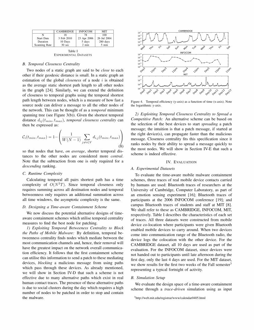
Figure 4. Temporal efficiency (y-axis) as a function of time (x-axis). Notethe logarithmic y-axis.

2) Exploiting Temporal Closeness Centrality to Spread aCompetitive Patch: An alternative scheme can be based onthe selection of the best devices to start spreading a patchmessage; the intuition is that a patch message, if started atthe right device(s), can propagate faster than the maliciousmessage. Closeness centrality fits this specification since itranks nodes by their ability to spread a message quickly tothe most nodes. We will show in Section IV-E that such ascheme is indeed effective.

IV. EVALUATION

A. Experimental Datasets

To evaluate the time-aware mobile malware containmentschemes, three traces of real mobile device contacts carriedby humans are used: Bluetooth traces of researchers at theUniversity of Cambridge, Computer Laboratory, as part ofan emotion sensing experiment [16]; Bluetooth traces ofparticipants at the 2006 INFOCOM conference [19]; andcampus Bluetooth traces of students and staff at MIT [8].We shall refer to these as CAMBRIDGE, INFOCOM, MIT,respectively. Table I describes the characteristics of each setof traces. All three datasets were constructed from mobiledevice co-location where participants were given Bluetoothenabled mobile devices to carry around. When two devicescome into communication range of the Bluetooth radio, thedevice logs the colocation with the other device. For theCAMBRIDGE dataset, all 10 days are used as part of theevaluation. For the INFOCOM dataset, since devices werenot handed out to participants until late afternoon during thefirst day, only the last 4 days are used. For the MIT dataset,we show results for the first two weeks of the Fall semester3

representing a typical fortnight of activity.

B. Simulation Setup

We evaluate the design space of a time-aware containmentscheme through a trace-driven simulation using as input

3http://web.mit.edu/registrar/www/calendar0405.html

12am 6am 12pm 6pm 12amTime

0.0

0.25

0.5

0.75

1.0

% N

odes

Infe

cted

Base[12.467]

Temporal Bet[11.062]

Static Bet[12.016]

Temporal Clos[12.041]

Static Clos[12.243]

12am 6am 12pm 6pm 12amTime

0.0

0.25

0.5

0.75

1.0

% N

odes

Infe

cted

Base[12.467]

Temporal Bet[7.446]

Static Bet[8.636]

Temporal Clos[7.980]

Static Clos[9.575]

0.0 0.2 0.4 0.6 0.8 1.0Patched Nodes (%)

0.0

6.0

12.0

18.0

24.0

Are

a U

nder

Curv

e

Temporal Bet

Static Bet

Temporal Clos

Static Clos

0.0 0.2 0.4 0.6 0.8 1.0Patched Nodes (%)

0.0

0.25

0.5

0.75

1.0

Final in

fect

ed n

odes

(%) Temporal Bet

Static Bet

Temporal Clos

Static Clos

Figure 5. INFOCOM day 4: Immunising 1 (top left) & 10 source nodes(top right). Area under curves shown in the legend. Area (bottom left) andfinal % of infected nodes (bottom right), as we increase the % of nodesimmunised (x-axis).

the three datasets described above. We will examine theeffects of four key factors: the starting time of the malwarespreading process tm and of the corresponding patching timetp, the initial number of the infected nodes Nm and theinitial number of patched nodes Np. The top Np devicesare chosen according to the calculated temporal betweennessor temporal closeness centrality ranking from the temporalgraph Gw(tp, tmax), where w is set to the finest windowgranularity, corresponding to the scanning rate of the devicesin each dataset (e.g., 30 second windows for CAMBRIDGE).The Nm nodes that are initially infected with maliciousmessages are chosen uniformly randomly. The results areobtained by averaging over 100 runs for each Np. The staticcentralities from the static aggregated graph over the timeinterval [tp, tmax] are also calculated for comparison.

Our evaluation is based on the following assumptions:firstly, when a node receives a patch message, it is im-munised for the rest of the simulation (i.e., we assumethat the malware does not mutate over time); secondly,there is always a successful file transfer between devices(errors in transmission can be taken into consideration inthe assessment of the contention scheme without changingsignificantly the results of our work, assuming randomtransmission failures); thirdly, an attacker chooses nodes atrandom; and finally, we have no knowledge of which devicesare compromised (otherwise the best scheme is to patchthose devices immediately).

C. Effects of Time on Malware Spreading

Firstly, we briefly analyse the effects of the time of dayhave on mobile malware propagation. Let us consider Fig-ure 4 where we measure the temporal efficiency (Formula 5)as a function of time. This sliding temporal efficiency iscalculated for all three datasets. As we can see there areoscillations corresponding to the natural human periodicdaily and weekly behaviour. For example, the CAMBRIDGE

Figure 6. INFOCOM: Temporal clustering provide four types of alternativepaths: (A) inflowing paths to temporal cluster; (B) redundant nodes incluster; (C) alternative flows around temporal cluster; (D) many outflowsto next temporal cluster.

dataset is spread over 10 days, and it is apparent from thetraces that a (malicious) message can spread more efficientlyduring the daytime, as opposed to evenings and weekends.

D. Non-Effectiveness of Betweenness based Patching

Starting from the results of the analysis of the effects timeof day has on message spreading, we now evaluate the bestcase scenario for the containment scheme based on patchingnodes (without spreading the patch) and we show that thisis highly inefficient since it requires a very large number ofnodes to be patched via the cellular network to be effective.

Using Day 4 of the INFOCOM trace for this example,a piece of malware is started at the beginning of the day(tm=12am) and the device(s) are patched at the same time(tp=12am). This is the best case scenario for two reasons:first, the temporal graph in the morning is characterised bylow temporal efficiency since there are very few contacts,therefore, the malware spreads slowly (as we have seen inFigure 4); secondly, devices that are immunised immediatelyhave the best chance of blocking malware spreading routes.

Figure 5 shows the ratio of compromised devices acrosstime when the top 1 (top left panel) and top 10 (topright panel) devices are patched after being selected usingbetweenness and closeness. As we can see, temporal be-tweenness initially performs better than static betweennessand both temporal and static closeness (quantified by thedifference in the area under each curve, shown in the legend).However, by 7am we observe a steep rise in the numberof compromised devices and by the end of the day, allcurves converge to the same point. We also note that inboth cases it is not possible to totally contain the malware,suggesting that more devices need to be patched. Takinga broader view, Figure 5 shows the area under the curve(bottom left) and final ratio of nodes infected (bottom right)as we increase the number of patched devices. Clearly,

even when the malware is started at the slowest time ofday for communication, we still need to patch 80% of thedevices before we can completely stop the malware fromspreading; this can be considered an impractically highnumber of devices to patch. Similar high percentages arealso required in the MIT trace with a minimum of 45%patched nodes. We can also conclude that in human contactnetworks, even with blocked nodes, it is only a matterof time before a (malicious) message disseminates to allnodes. To understand the reason for the effectiveness of a(malicious) message propagation, we take a visual analysisapproach: Figure 6 shows the temporal activity diagram4

for the INFOCOM experiment across all four days. Thisgives a bird’s eye view of proximity between individuals asthey move between groups of colocated people across time,where the trajectory of the same node is given by a straightline. The horizontal axis is time and the vertical groupings ofnodes represents people that are in the same static connectedcomponent such that there is a path between every node inthat cluster. The main feature to note is the temporal clusterof remarkable size which appears from around 7am until7pm every day, coinciding with the main activities at theINFOCOM conference5. By means of this infographic, whatwe see are periodic clusters of nodes during the daytime andsmaller disparate clusters during the evening. Figure 6 alsozooms into Day 4, highlighting the four types of activitywhich give rise to temporal clustering and more importantly,to alternative paths providing link redundancy for a messageto pass through a network over time. Since this strategycannot deal with these alternative paths effectively, thepropagation of a malicious message can merely be sloweddown. Hence, the rapid increase of infected nodes that canbe observed in Figure 5 around 7am can be attributed tothe presence of this large temporal cluster starting at 7amwhere many alternative paths are present and, therefore, thespreading cannot be stopped just patching some of the nodes.We conclude that this containment strategy is not efficientgiven the large number of patch messages it requires.

E. Effectiveness of Closeness based Patching (Worst CaseScenario)

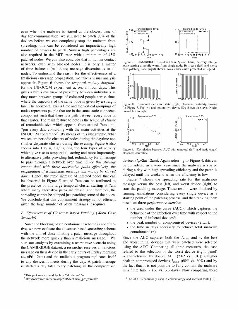
Since the blocking based containment scheme is not effec-tive, we now evaluate the closeness based spreading schemewith the aim of disseminating a patch message throughoutthe network more quickly than a malicious message. Westart our analysis by examining a worst case scenario usingthe CAMBRIDGE dataset: a researcher receives a maliciousmessage on their device in the early hours of Friday morning(tm=Fri 12am) and the malicious program replicates itselfto any devices it meets during the day. A patch messageis started a day later to try patching all the compromised

4This plot was inspired by http://xkcd.com/6575http://www.ieee-infocom.org/2006/technical program.htm

W T F S S M T W T F STime

0.0

0.5

1.0

Nodes

Reach

ed (

%)

Patched Node ID=17Patch [5.33]

Malware [1.14]

W T F S S M T W T F STime

0.0

0.5

1.0

Nodes

Reach

ed (

%)

Patched Node ID=11Patch [3.57]

Malware [2.62]

Figure 7. CAMBRIDGE [tm=Fri 12am, tp=Sat 12am] delivery rate (y-axis) starting a mobile worm from single node. Best case (left) and worsecase patching node (right) shown. Area under curve presented in legend.

0.0

0.5

1.0

Tem

pora

l C

lose

ness

017, 010, ..., 011, 0090.0

0.5

1.0

Sta

tic

Clo

seness

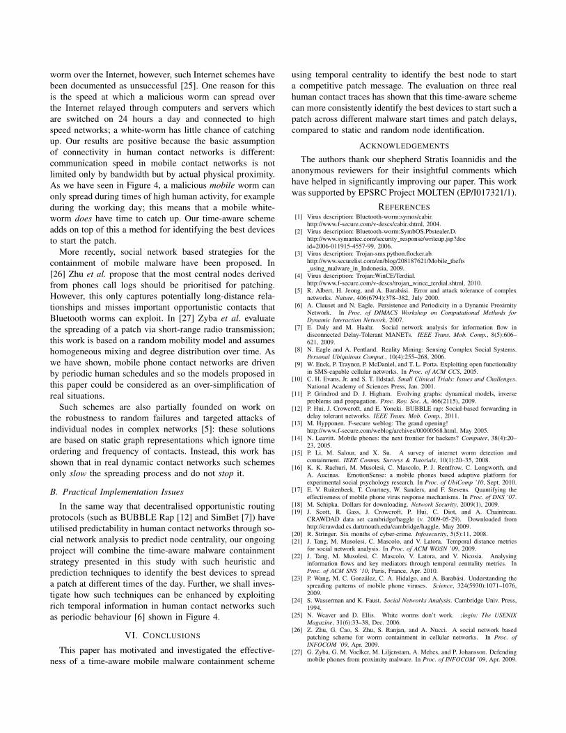
010, 017, ..., 016, 018

Figure 8. Temporal (left) and static (right) closeness centrality rankingfor Figure 7. Top two and bottom two device IDs shown on x-axis. Nodesranked left to right.

0.0 0.8 1.6 2.4AUC

0.0

0.5

1.0

Tem

pora

l C

lose

ness

Spearman=-0.62

0.0 0.8 1.6 2.4AUC

0.0

0.5

1.0

Sta

tic

Clo

seness

Spearman=0.33

Figure 9. Correlation between AUC with temporal (left) and static (right)closeness centrality.

devices (tp=Sat 12am). Again referring to Figure 4, this canbe considered as a worst case since the malware is startedduring a day with high spreading efficiency and the patch isdelayed until the weekend when the efficiency is low.

Figure 7 shows the spreading rate for the maliciousmessage versus the best (left) and worst device (right) tostart the patching message. These results were obtained byrunning simulations considering every single device as astarting point of the patching process, and then ranking thembased on three performance metrics:• the area under the curve (AUC), which captures the

behaviour of the infection over time with respect to thenumber of infected devices6;

• the peak number of compromised devices (Imax);• the time in days necessary to achieve total malware

containment (τ ).Since the AUC captures both the Imax and τ , the bestand worst initial devices that were patched were selectedusing the AUC. Comparing all three measures, the caserelated to the selection of the worst device (right panel)is characterised by double AUC (2.62 vs. 1.07); a higherpeak in compromised devices Imax (68% vs. 60%) and bythe fact that it is not possible to fully contain the malwarein a finite time τ (∞ vs. 3.3 days). Now comparing these

6The AUC is commonly used in epidemiology and medical trials [10].

CAMBRIDGE

0

1

2

AUC

0

4

8

12

τ

WedTh

u Fri

SatSu

nMon Tu

eW

edThu Fr

i0.00

0.25

0.50

0.75

Imax

RAND

T Clos

S Clos

T Bet

S Bet

INFOCOM

0.0

0.5

1.0

AUC

1

2

3

4

τ

Day2

Day3

Day4

Day5

0.0

0.4

0.8

Imax

RAND

T Clos

S Clos

T Bet

S Bet

MIT

0

1

2

AUC

3

6

9

12

τ

Day0Day

1Day

2Day

3Day

4Day

5Day

6Day

7Day

8Day

9

Day10

Day11

Day12

Day13

0.0

0.2

0.4

Imax

RAND

T Clos

S Clos

T Bet

S Bet

Figure 10. Performance of temporal, static and naive node selection, across different malware start times (x-axis), averaged over all patch delays.

observations with centrality, in Figure 8 we observe thatthe node characterised by the highest temporal closenesscentrality (ID=17) is also the optimal one for spreadingthe patch and the node that leads to the worst performance(ID=11) is ranked within the bottom two nodes. This shouldbe compared with static centrality which ranks the bestdevice to start the patching process (ID=17) in second placeand the worst device (ID=11) seventh from the bottom (notshown). Also, the values of static centrality of each node ismore uniformly distributed; a fact which can be attributed tothe dense static graph previously observed in Figure 1. Thestronger correlation between temporal closeness centralityand an effective malware containment scheme can be seenmore clearly by plotting these rankings against the AUCin Figure 9. We expect a strong negative correlation sincecentrality values are ranked in descending order; by usingtemporal closeness centrality, we can identify the best nodeto start disseminating a patch message to contain a pieceof mobile malware which fits our intuition that spreading apatch message quickly is the best containment strategy.

F. Effects of Temporal Variability

Thus far we have only considered a single malware starttime. We now take a broader view and examine the effectsof varying malware start time (tm) and patch delay (tp). Foreach dataset the AUC, Imax and τ are exhaustively calcu-lated for different malware start times at hourly intervalsand increasing patch delays starting from zero (i.e., patchmessages start at the same time as malicious messages) to upto 2 days. We compare node selection based on temporal andstatic closeness to that of temporal and static betweenness.As a baseline, a naive method of randomly selecting patchingnodes is also calculated, averaged over 100 runs.

1) Sensitivity to Malware Start Time: To understand theeffects of a malicious message starting at different times,Figure 10 shows for each dataset the performance metricsas a function of the malware start time tm, averaged overall patch delays. Firstly, referring back to the temporalefficiency from Figure 4, which exhibited daily peaks and

troughs during the weekend, the AUC and the maximumnumber of infected nodes Imax tend to follow these samepatterns (strictly related to human circadian rhythms); how-ever, the total time of containment (τ ) remains stable acrossall start times. These results demonstrate that this time-awarecontainment scheme is an effective method of quickly con-taining malware, irrespective of when the malware started.Now analysing the AUC and Imax, the temporal closenesscentrality curve is consistently lower than static closeness,betweenness (both temporal and static) and naive methods.Further, betweenness (both static and temporal) generallytake longer to fully contain the malware (higher values ofτ ) and static closeness centrality performs worse than thenaive method at some points of time; more specifically:• For the CAMBRIDGE dataset, during the weekend a

static closeness method has a higher peak number ofcompromised devices (Imax) than the naive method,which shows that a static method is not effective atslowing down the malware from spreading.

• For the INFOCOM dataset, again Imax is higher thanthe naive method, during days 2 and 4. In addition, theAUC curve for a static method peaks with temporalefficiency during days 2, 4 and 5: this means that themalware is not contained effectively in these scenarios.Also, the total containment time (τ ) is greater than thatof the naive method during days 3, 4 and 5. This showsthat temporal closeness centrality is more consistent atidentifying the best nodes to start the patching process,compared to both static and naive methods.

• Finally, for the MIT dataset, the naive method performsextremely poorly (with high values of AUC, Imax andτ across all malware start times), compared to either astatic or temporal methods. However, we also see thatduring the first week of the Fall semester, temporalcloseness centrality identifies nodes with lower AUCand τ , exhibiting over half a day quicker malwarecontainment compared to static closeness centrality.

2) Sensitivity to Patch Delay: To understand the effectsof delaying a patch message after a malware outbreak,

CAMBRIDGE

0

1

2

3

AUC

0

3

6τ

0sec

15m

ins

30m

ins

1hr

3hrs

12hr

s

1day

s

1.5d

ays

2day

s0.0

0.3

0.6Imax

T Clos

S Clos

T Bet

S Bet

RAND

INFOCOM

0

1

2AUC

0.0

1.5

3.0τ

0sec

15m

ins

30m

ins

1hr

3hrs

12hr

s

1day

s

1.5d

ays

2day

s0.0

0.4

0.8Imax

MIT

0.0

0.8

1.6AUC

0

4

8τ

0sec

15m

ins

30m

ins

1hr

3hrs

12hr

s

1day

s

1.5d

ays

2day

s0.00

0.15

0.30Imax

Figure 11. Performance of temporal, static and naive node selection methods, as a function of patch delay (x-axis), averaged over all malware start times.

Figure 11 plots the performance metrics for a representativesample of patch delays, averaged over all malware starttimes. As the patch delay increases, all the performanceindicators also increase. However, we note that across allthree datasets, temporal closeness centrality (left most bar)exhibits the best results: smallest AUC, fastest total con-tainment time (τ ) and smallest peak compromised devices(Imax). We also observe that in the INFOCOM dataset,static closeness node selection gives higher values of Imax

and τ up to a 12 hour delay, showing that static centralitydoes not consistently capture the true speed at which anode can spread a message, compared to temporal closenesscentrality. Also, these plots demonstrate that betweenness(both static and temporal) are not suited to a spreadingprocess and hence perform worse than closeness based nodeselection. Again, from these observations, we conclude that acontainment scheme based on temporal closeness centralityprovides the best performance as the patch delay increases.

G. Impact of the Initial Number of Compromised and Patch-ing Devices

We now look at the effects of starting malware messages(Nm) and patch messages (Np) from more than one device.This corresponds to the case, for example, when a groupof people download a malicious program at the same time,or an attacker has programmed the replication to be time-triggered. Since we have observed that betweenness basednode selection is not suited to patch spreading scheme, wenow focus on closeness based node selection only. To makecomparisons with the first containment scheme (SectionIV-D) we discuss result for the same malware start andpatch delay times. Similar trends were found for differentstart times and other datasets. Figure 12 shows the effectof starting a patch from an increasing number of initialdevices Np (increasing column left to right) as the number ofinitially compromised devices Nm (reported on the x-axis)is increased for the INFOCOM dataset.

First, in the case when a single initial patch message(Np=1) is used (left panel), we observe that the AUCcorresponding to the scheme based on temporal centralityis lower than that corresponding to the cases of static and

0 0.5 1Nm (%)

0

Np=1node

0.00

0.15

0.30AUC

0.0

0.6

1.2τ

0.0

0.4

0.8

Imax

RAND

Temporal

Static

0 0.5 1Nm (%)

0.0

0.4

0.8

Np=10%

0.00

0.15

0.30

0.0

0.6

1.2

0 0.5 1Nm (%)

0.0

0.4

0.8

Np=25%

0.00

0.15

0.30

0.0

0.6

1.2

0 0.5 1Nm (%)

0.0

0.4

0.8

Np=50%

0.00

0.15

0.30

0.0

0.6

1.2

Figure 12. INFOCOM: Effect of increasing number of initial deviceswith malware (x-axis). From left to right, each column plots an increasingnumber of devices from which a patch is started (tm=tp=Day 4 12am).

naive methods of node selection even as Nm increases;the total containment time (τ ) remains below half a dayup to Nm=75% of the total number of nodes (which weindicate with Ntot) and the peak compromised devices(Imax) rises slowly as Nm increases. When increasing toNp=10%Ntot, using temporal centrality the total contain-ment time (Imax) drops below 2.5 hours (about 0.1 of aday) up to Nm=75%Ntot. Only at Np=25%Ntot both thenaive and static methods start to match the performance ofthe temporal method. These observations suggest that ourtime-aware containment scheme using temporal centrality ismore accurate at ranking important nodes and hence a viableoption for a network operator since less devices are requiredto receive a patching message in order to achieve an effectivecontainment strategy.

V. DISCUSSION

A. Related Work

The study of techniques for containing the spreading ofviruses and malware in the Internet has a long tradition (see arecent survey by Li et al. [15]). However, traditional desktopand server techniques for malware containment involve virusscanners running on a computer; such a scheme is notfeasible on many mobile devices with limited resources.More related to our work are so called “white-worms” whichpropagate themselves in the same fashion as a malicious

worm over the Internet, however, such Internet schemes havebeen documented as unsuccessful [25]. One reason for thisis the speed at which a malicious worm can spread overthe Internet relayed through computers and servers whichare switched on 24 hours a day and connected to highspeed networks; a white-worm has little chance of catchingup. Our results are positive because the basic assumptionof connectivity in human contact networks is different:communication speed in mobile contact networks is notlimited only by bandwidth but by actual physical proximity.As we have seen in Figure 4, a malicious mobile worm canonly spread during times of high human activity, for exampleduring the working day; this means that a mobile white-worm does have time to catch up. Our time-aware schemeadds on top of this a method for identifying the best devicesto start the patch.

More recently, social network based strategies for thecontainment of mobile malware have been proposed. In[26] Zhu et al. propose that the most central nodes derivedfrom phones call logs should be prioritised for patching.However, this only captures potentially long-distance rela-tionships and misses important opportunistic contacts thatBluetooth worms can exploit. In [27] Zyba et al. evaluatethe spreading of a patch via short-range radio transmission;this work is based on a random mobility model and assumeshomogeneous mixing and degree distribution over time. Aswe have shown, mobile phone contact networks are drivenby periodic human schedules and so the models proposed inthis paper could be considered as an over-simplification ofreal situations.

Such schemes are also partially founded on work onthe robustness to random failures and targeted attacks ofindividual nodes in complex networks [5]: these solutionsare based on static graph representations which ignore timeordering and frequency of contacts. Instead, this work hasshown that in real dynamic contact networks such schemesonly slow the spreading process and do not stop it.

B. Practical Implementation Issues

In the same way that decentralised opportunistic routingprotocols (such as BUBBLE Rap [12] and SimBet [7]) haveutilised predictability in human contact networks through so-cial network analysis to predict node centrality, our ongoingproject will combine the time-aware malware containmentstrategy presented in this study with such heuristic andprediction techniques to identify the best devices to spreada patch at different times of the day. Further, we shall inves-tigate how such techniques can be enhanced by exploitingrich temporal information in human contact networks suchas periodic behaviour [6] shown in Figure 4.

VI. CONCLUSIONS

This paper has motivated and investigated the effective-ness of a time-aware mobile malware containment scheme

using temporal centrality to identify the best node to starta competitive patch message. The evaluation on three realhuman contact traces has shown that this time-aware schemecan more consistently identify the best devices to start such apatch across different malware start times and patch delays,compared to static and random node identification.

ACKNOWLEDGEMENTS

The authors thank our shepherd Stratis Ioannidis and theanonymous reviewers for their insightful comments whichhave helped in significantly improving our paper. This workwas supported by EPSRC Project MOLTEN (EP/I017321/1).

REFERENCES[1] Virus description: Bluetooth-worm:symos/cabir.

http://www.f-secure.com/v-descs/cabir.shtml, 2004.[2] Virus description: Bluetooth-worm:SymbOS.Pbstealer.D.

http://www.symantec.com/security response/writeup.jsp?docid=2006-011915-4557-99, 2006.

[3] Virus description: Trojan-sms.python.flocker.ab.http://www.securelist.com/en/blog/208187621/Mobile theftsusing malware in Indonesia, 2009.

[4] Virus description: Trojan:WinCE/Terdial.http://www.f-secure.com/v-descs/trojan wince terdial.shtml, 2010.

[5] R. Albert, H. Jeong, and A. Barabasi. Error and attack tolerance of complexnetworks. Nature, 406(6794):378–382, July 2000.

[6] A. Clauset and N. Eagle. Persistence and Periodicity in a Dynamic ProximityNetwork. In Proc. of DIMACS Workshop on Computational Methods forDynamic Interaction Network, 2007.

[7] E. Daly and M. Haahr. Social network analysis for information flow indisconnected Delay-Tolerant MANETs. IEEE Trans. Mob. Comp., 8(5):606–621, 2009.

[8] N. Eagle and A. Pentland. Reality Mining: Sensing Complex Social Systems.Personal Ubiquitous Comput., 10(4):255–268, 2006.

[9] W. Enck, P. Traynor, P. McDaniel, and T. L. Porta. Exploiting open functionalityin SMS-capable cellular networks. In Proc. of ACM CCS, 2005.

[10] C. H. Evans, Jr. and S. T. Ildstad. Small Clinical Trials: Issues and Challenges.National Academy of Sciences Press, Jan. 2001.

[11] P. Grindrod and D. J. Higham. Evolving graphs: dynamical models, inverseproblems and propagation. Proc. Roy. Soc. A, 466(2115), 2009.

[12] P. Hui, J. Crowcroft, and E. Yoneki. BUBBLE rap: Social-based forwarding indelay tolerant networks. IEEE Trans. Mob. Comp., 2011.

[13] M. Hypponen. F-secure weblog: The grand opening!http://www.f-secure.com/weblog/archives/00000568.html, May 2005.

[14] N. Leavitt. Mobile phones: the next frontier for hackers? Computer, 38(4):20–23, 2005.

[15] P. Li, M. Salour, and X. Su. A survey of internet worm detection andcontainment. IEEE Comms. Surveys & Tutorials, 10(1):20–35, 2008.

[16] K. K. Rachuri, M. Musolesi, C. Mascolo, P. J. Rentfrow, C. Longworth, andA. Aucinas. EmotionSense: a mobile phones based adaptive platform forexperimental social psychology research. In Proc. of UbiComp ’10, Sept. 2010.

[17] E. V. Ruitenbeek, T. Courtney, W. Sanders, and F. Stevens. Quantifying theeffectiveness of mobile phone virus response mechanisms. In Proc. of DNS ’07.

[18] M. Schipka. Dollars for downloading. Network Security, 2009(1), 2009.[19] J. Scott, R. Gass, J. Crowcroft, P. Hui, C. Diot, and A. Chaintreau.

CRAWDAD data set cambridge/haggle (v. 2009-05-29). Downloaded fromhttp://crawdad.cs.dartmouth.edu/cambridge/haggle, May 2009.

[20] R. Stringer. Six months of cyber-crime. Infosecurity, 5(5):11, 2008.[21] J. Tang, M. Musolesi, C. Mascolo, and V. Latora. Temporal distance metrics

for social network analysis. In Proc. of ACM WOSN ’09, 2009.[22] J. Tang, M. Musolesi, C. Mascolo, V. Latora, and V. Nicosia. Analysing

information flows and key mediators through temporal centrality metrics. InProc. of ACM SNS ’10, Paris, France, Apr. 2010.

[23] P. Wang, M. C. Gonzalez, C. A. Hidalgo, and A. Barabasi. Understanding thespreading patterns of mobile phone viruses. Science, 324(5930):1071–1076,2009.

[24] S. Wasserman and K. Faust. Social Networks Analysis. Cambridge Univ. Press,1994.

[25] N. Weaver and D. Ellis. White worms don’t work. ;login: The USENIXMagazine, 31(6):33–38, Dec. 2006.

[26] Z. Zhu, G. Cao, S. Zhu, S. Ranjan, and A. Nucci. A social network basedpatching scheme for worm containment in cellular networks. In Proc. ofINFOCOM ’09, Apr. 2009.

[27] G. Zyba, G. M. Voelker, M. Liljenstam, A. Mehes, and P. Johansson. Defendingmobile phones from proximity malware. In Proc. of INFOCOM ’09, Apr. 2009.