
Explicit and Implicit Incentives: Longitudinal Evidence … research does not distinguish between...
31
Explicit and Implicit Incentives: Longitudinal Evidence from NCAA Football Head Coaches Employment Contracts Presented by Dr Brian Cadman Assistant Professor University of Utah # 2013/14-17 The views and opinions expressed in this working paper are those of the author(s) and not necessarily those of the School of Accountancy, Singapore Management University.
Transcript of Explicit and Implicit Incentives: Longitudinal Evidence … research does not distinguish between...

Explicit and Implicit Incentives:
Longitudinal Evidence from NCAA Football Head Coaches Employment Contracts
Presented by
Dr Brian Cadman
Assistant Professor University of Utah
# 2013/14-17
The views and opinions expressed in this working paper are those of the author(s) and not necessarily those of the School of Accountancy, Singapore Management University.

Explicit and Implicit Incentives: Longitudinal Evidence from NCAA Football Head
Coaches Employment Contracts
Brian Cadman
David Eccles School of Business, University of Utah
Gavin Cassar
INSEAD
Early draft: Please do not distribute
Abstract
We study the role of explicit and implicit incentives in a competitive labor market with no
internal promotion opportunities. We find that explicit incentives explain only a small fraction of
the total incentives, as the likelihood of new employment on better terms and renegotiation of
current employment on better terms increases following good performance. We also find the
likelihood of renegotiation versus changing employment on better terms is dependent on the
institutional characteristics and their willingness to pay in the market for labor. Our findings
demonstrate the role of renegotiation and the relative strength of labor market forces compared to
ex-ante pay-for-performance in the presence of strong external labor market incentives. Further,
our results suggest that conclusions regarding the optimal use of explicit incentives in pay-for-
performance may be substantially overstated when not considering the role of external labor
market incentives.

2
―The manager of a firm, like the coach of any team, may not suffer any immediate gain
or loss in current wages from the current performance of his team, but the success or failure of
the team impacts his future wages, and this gives the manager a stake in the success of the team.‖
Fama (1980) Journal of Political Economy, p.292.
1. Introduction
Explicit (contractible) and implicit (non-contractible) incentives motivate an agent’s
effort. For example, CEOs can be incentivized by ex-ante specified explicit bonus terms, or
implicitly incentivized by expectations of being ex-post settled-up by the board after observed
performance or by the presence of external labor markets that offer better future employment
terms. While understanding of the mix of total incentives is critical, outside of some notable
exceptions (e.g., Gibbons and Murphy, 1992; Rajgopal, Shevlin and Zamora, 2006), much of the
prior research does not distinguish between ex-ante and ex-post determined compensation or
consider the role of implicit external labor market incentives when determining the optimal use
of explicit incentives. Evidence on the importance of explicit and implicit incentives is limited
due to a lack of observability of explicit incentives and subsequent renegotiation (Gillan, Hartzell
and Parrino, 2009: 1630), difficulty to observe career outcomes beyond current employment, and
a lack of precision of expected implicit incentives associated with career concerns. To provide
evidence on implicit incentives in contracting, we use the labor market for National Collegiate
Athletic Association (NCAA) football head coaches. We investigate how the implicit incentives
from external labor market forces affect the use and importance of explicit incentives in
compensation.
We report three important findings. First, we document the characteristics and magnitude
of explicit incentives in head coaches’ contracts. We observe the mean (median) maximum
explicit incentives for head coaches to be 36% (29%) of the total fixed component of

3
compensation. Inconsistent with the arguments of Gibbons and Murphy (1992), we find no
evidence that the relative magnitude of explicit incentives is greater when implicit incentives
from external hiring are weakest.
Second, we compare the actual change in head coach compensation with the explicit
compensation change specified in the employment contract. Examining coaches that remain in
their current employment, a common research design choice used by researchers when
examining CEO total incentives, we find the mean (median) actual change in year-to-year
compensation to be 24% (3%). However, we find substantial differences in compensation driven
by successful head coaches either accepting new employment or renegotiating their existing
employment contract on better terms, which occurs 26% and 33% on average each coach-year,
respectively. For example, coaches who renegotiate their existing contract experience a mean
(median) actual change in compensation of 75% (33%) compared to a mean (median) change of
-1% (1%) for those that do not renegotiate. More striking, when we examine coaches who move
to other institutions, we find these coaches experience a mean (median) actual change in
compensation of 264% (257%). Therefore, we demonstrate that excluding head coaches that do
not remain in their current employment year-to-year substantially understates the true
relationship between performance and pay.
Third, we model the likelihood of a head coach voluntarily terminating their current
employment to accept higher paid employment or renegotiating their existing employment
contract on better terms. We find that renegotiation is more likely when the team performs well
(high winning percentage or appearing in the national championship game in previous year) and
when the college is large (BCS institution, higher salary rank) and therefore has limited
competitors that would dominate their willingness to pay for the coach’s talent. This evidence is

4
consistent with Gibbons and Murphy (1992: 470) conjecture that renegotiation mimics one of the
effects of labor market competition. We observe the probability of higher paid employment
(institution change) is also significantly more likely when the coaches’ team performs well (high
winning percentage); however, the likelihood of institution change decreases with college size
(stadium capacity). Taken together, this suggests that relatively smaller colleges are less able or
willing to increase pay sufficiently (renegotiate) to retain better performing coaches, and that a
equilibrium exists where institutions that reap the greatest returns to performance attract and
retain the most talented coaches. We examine three alternative arguments to this small
college/large college equilibrium pay explanation: 1) that departing coaches are lesser paid in
their original employment; 2) that new colleges overpay for head coaches from other colleges;
and 3) that the original colleges would have provided this pay increase. We find no support for
any of these alternative explanations. Overall, our results show how implicit incentives become
reflected in agent compensation – either within the firm or through the external labor market – is
dependent on the characteristics of the institution that employ the coach and the market for their
labor.
Our findings provide insight on a fundamental question of labor contracting in the
presence of only external labor market incentives (no promotion opportunities). We show that in
the presence of strong external labor market incentives, explicit pay-for-performance is of
limited importance. Our evidence provides bounds for workers in other labor markets with no
internal promotion opportunities, such as CEOs, where data availability inhibit empirical
investigation of labor market contracting. Overall, we demonstrate that in the presence of strong
external incentives and renegotiation that implicit incentives (limited explicit pay-for-

5
performance) can optimally incentive workers, where a small college/large college equilibrium
exists for agent talent.
2. Research Question and Setting
2.1 Related literature
Agent effort is motivated through total incentives, which can consist of ex-ante specified
explicit or contractible incentives, and implicit or non-contractible incentives, such as the
expectation of being ex-post settled-up (compensated) by the principal after observed
performance, or an improvement of the likelihood of future promotion or better employment
terms within the firm or in the external market for labor. Yet, almost all evidence of agent
incentives, particularly CEOs, is predominately limited to the relation between organizational
performance and observable changes in wealth experienced by the agent, which may be an
outcome of explicit or implicit incentives. Further, researchers generally exclude agents that
either choose to leave or are fired from their employment – as agents must be observed in
consecutive periods to estimate the performance-pay relation within current employment – and
even for those agents that remain in their current employment, researchers generally do not
observe when explicit performance is rewarded, ex-post settling up has occurred, or
renegotiation has taken place. The primary reason for the lack of empirical investigation of the
mix of total incentives is the difficulty in observing these forces in most labor market settings.
While the relative importance of explicit and implicit incentives is generally excluded
from empirical investigations of pay and performance, there have been some notable exceptions
that have considered the interplay between explicit and implicit incentives. Gibbons and Murphy
(1992) posit and find that explicit incentives are stronger for CEOs nearing retirement, as the
6
implicit incentives from career concerns are weakest for these CEOs. Rajgopal, Shevlin and
Zamora (2006) find evidence consistent with the Oyer (2004) model that more talented CEOs
will have greater pay sensitivity to market-wide factors as they have greater external labor
market opportunities. Ederhof (2011) find that explicit bonus-based incentives are greater for
mid-level managers that face weaker implicit incentives from internal promotion. Again, while
these and other investigations provide insight into explicit and implicit incentive trade-offs, this
research does not consider the relative importance of alternative incentives or differences
between explicit incentives and ex-post settling up, nor do they consider agents that self-select
for better employment outside the firm. To provide insight into these important issues, we
examine a well-defined labor market where performance is more easily observable, contract
terms that link pay with performance are measurable, the labor market is more clearly defined,
and talent transfers across organizations more easily.
2.2 The labor market for NCAA head coaches
Sports labor markets have several empirical advantages to investigate incentives over
other labor markets, such as the market for CEOs (Kahn, 2000). First, unlike CEOs, almost all
NCAA coaches’ contracts are publicly observable (Gillian, Hartzell and Parrino, 2009), which
allows us to empirically distinguish between the ex-ante explicit incentives and any ex-post
settling up from renegotiation in actual pay outcomes (Fee, Hadlock and Pierce, 2006). By
observing renegotiation we do not require the commonly used assumption that employment
contracts are renegotiation proof (Gibbons and Murphy 1992: 470). Further, unlike CEOs,
coaches do not own stock in their institutions, which allows for more precise estimation of total
incentives in compensation and the separation of ownership and control is transparent.

7
Second, NCAA coaches are in a well-defined competitive labor market, which allows for
more accurate estimations of career concerns from labor market-based incentives. Within this
market we can observe coaches career outcomes over time, including transfer between colleges
and professional leagues, which is relatively common as coaches possess transferable talent with
limited institution-specific capital (Dutta, 2008). This longer period of observation recognizes
that several years are necessary to capture the dynamics in the pay-performance relation
(Boschen and Smith, 1995). While there is some research on job outcomes following
employment, such as senior officers of public firms (e.g., Brickley, Linck, and Coles, 1999;
Chang, Dasgupta and Hilary, 2010; Fee and Hadlock, 2004), it is difficult to observe the
employment terms for the majority of these workers.
Third, the performance metrics are well-defined and easy to observable, resulting in less
information asymmetry in the labor market and by researchers. Further, the timing of observed
performance and labor market outcomes (e.g., almost all turnover and renegotiation occurs at the
end of the football season) allows researchers to observe clear causal associations between
performance and compensation.
Finally, another important advantage of examining NCAA head coaches is an alternative
setting to CEOs to investigate incentives and contracting. The super majority of all empirical
research on incentives is based on the most senior officers of the largest publicly listed firms.
While significant focus on these officers’ incentives can be motivated by the importance of these
firms to the economy, there is lack of evidence from alternative settings, particularly settings that
are absent of regulation that affects organizations’ choice of incentives used. For example,
section 162(m) of the internal revenue code limits the tax deductibility of salaried compensation
to $1 million for senior officers of US publicly listed firms. This regulation makes it more costly
8
for these firms to use greater salaried compensation to incentivize workers, which likely distorts
the mix of incentives absent of this regulation.
3. Sample Selection and Variable Measurement
3.1 Sample
We examine employment contracts for head coaches of the NCAA Football Bowl
Subdivision (FBS). The FBS consists of 120 universities aligned in 11 conferences that each
range from 10-14 members and four independent teams with no conference affiliation (e.g. the
University of Notre Dame). Our sample spans contracts for the academic years beginning each
fall from 2006 to 2010, and include 107, 108, 110, and 109 teams in each year, respectively. The
omission of teams from the sample is due to the non-disclosure of employment contracts by
private institutions and a small subset of public institutions (e.g. the University of Southern
California). We collect several details from the contracts including annual salaried compensation
and explicit incentive bonuses, in addition to other contract terms, such as the contract length and
termination clauses.
Limiting the analysis to a homogenous labor market and setting removes heterogeneity in
the quality of available successors and ability to accurately assess coach performance (Parrino,
1997). Further, by focusing solely on head coaches we remove heterogeneity in decision-making
authority, variation in the extent of monitoring and any implicit incentives related to internal
promotion that may influence the use of explicit incentives (Ederhof, 2011). The lack of internal
promotion, in addition to other features, mirrors the implicit incentives in the labor market for
CEOs.
3.2 Compensation, Performance and Institution Measures
9
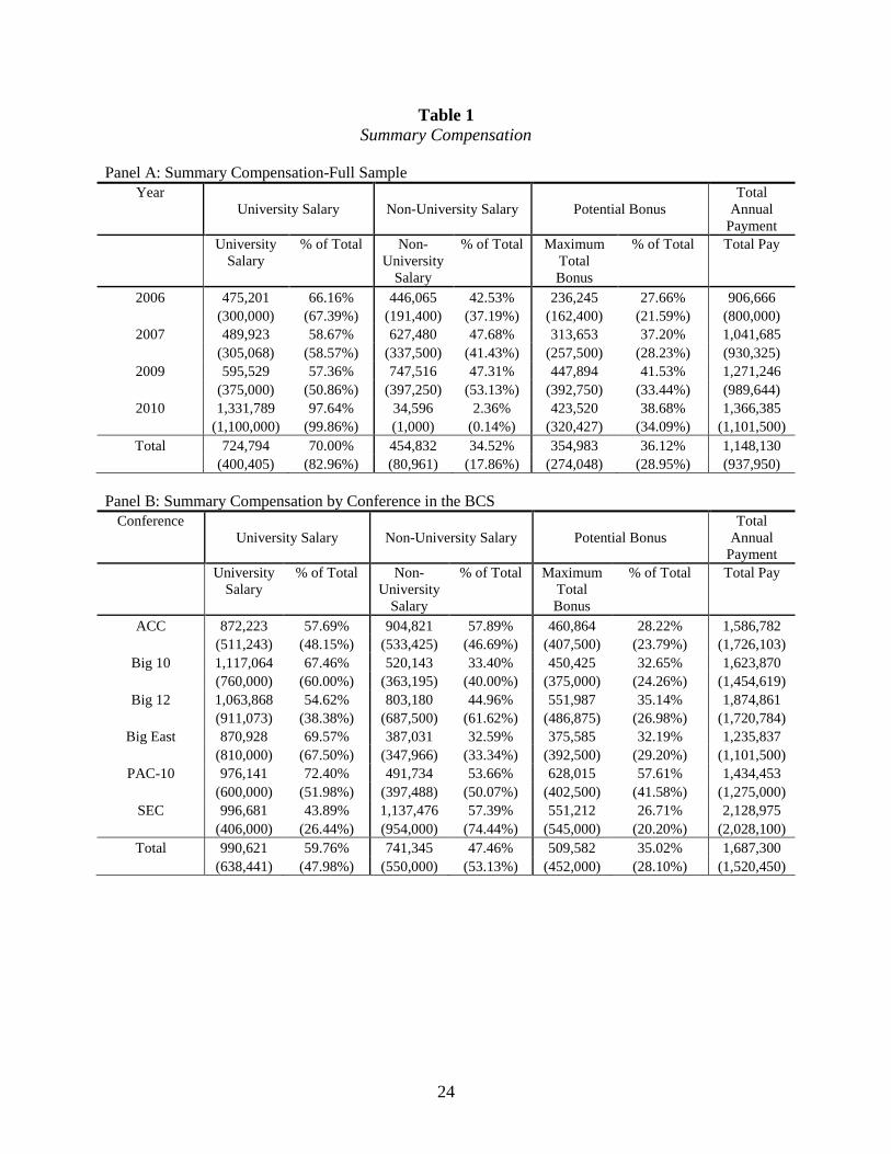
Table 1 Panel A provides summary statistics of annual compensation and the maximum
bonus the coach can earn. The mean (median) annual salary is $1,148,000 ($937,950), of which
70% (83%) is university-paid with the remaining sourced from other affiliates such as corporate
sponsors, university support groups or media organizations. The maximum bonus that an average
(median) coach can earn in a season is $354,983 ($274,048), which equates to a mean (median)
maximum potential bonus of 36% (29%) of their total salary. These bonuses include explicit
incentives associated with on-field performance (e.g. win-loss record, bowl appearances, national
and conference rankings) and off-field performance (e.g. graduation rates, attendance, etc.).
NCAA coaches’ compensation is increasing over our sample period, with the mean (median)
salaried compensation rising from $906,666 ($800,000) in 2006 to $1,366,385 ($1,101,500) in
2010. The nominal maximum potential bonus is also increasing over time such that the
proportion of maximum bonus to total salary increases slightly over the sample period.
Table 1 Panel B presents the summary compensation by athletic conference. We denote
the six Bowl Champion Series (BCS) conferences (ACC, Big 12, Big East, Big 10, Pac 10, and
SEC) that have greater access to more prestigious bowls and lucrative media rights compared to
the non-automatically qualifying (non-AQ) conferences. Consistent with BCS conference teams
attracting more talented coaches with greater reservation wages and a greater investment by the
University in the program, the mean (median) total salary for coaches of BCS teams of
$1,687,300 ($1,520,450) is significantly greater than the mean (median) total salary for non-AQ
coaches of $511,421 ($390,603). Despite the significant differences in salary between BCS and
non-AQ universities the maximum bonus as a percentage of total salary is not significantly
different, with the mean (median) bonus being 35% (28%) for BCS institutions and 37% (30%)
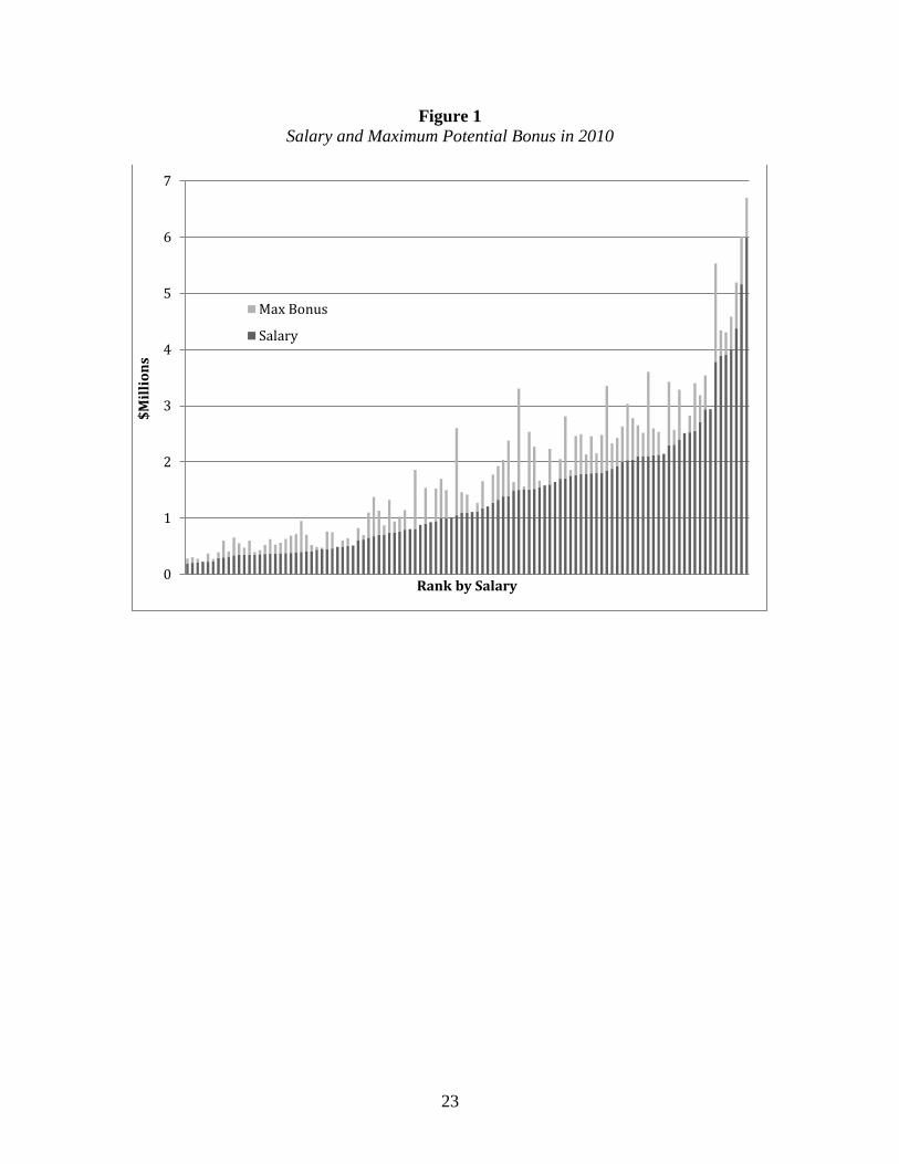
for non-AQ institutions. Figure 1 provides the salary and maximum bonus for all our coaches in
10
our most recent sample year (2010) ranked by total salary. This figure shows convexity in the
labor market salaries of NCAA football coaches. In fact, the average Pearson correlation
between total salary and the ranked salary for the NCAA football coach labor market in our
sample period is 0.98.
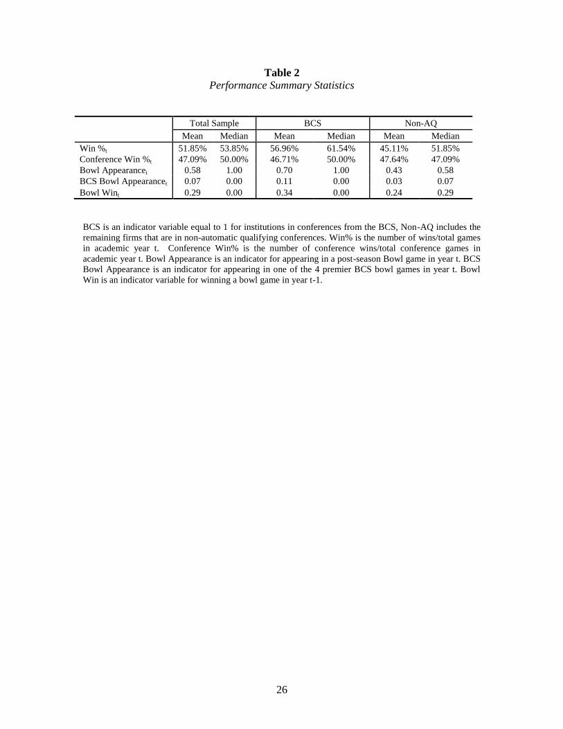
Table 2 provides the summary statistics of our performance measures. We obtain the
winning percentage, conference winning percentage, playing in a bowl game, playing in a BCS
bowl game, winning a bowl game, and appearing in the national championship game. Our
performance measures are motivated by their explicit use in our head coaches’ employment
contracts and by published research on football coach compensation, promotions and firings
(Fee, Hadlock, Pierce, 2006; Holmes, 2011). Consistent with BCS teams performing better than
Non-AQ teams, on average, the winning percentage of BCS teams is more than 10% greater than
non-AQ teams., In addition, BCS teams appear in post-season bowl games 70% of the time,
while non-AQ teams appear in a bowl game 43%. BCS teams also appear in BCS bowls and win
their bowl game more frequently than non-AQ teams.
We also measure the size of the college as it relates to their investment in the football
program. To measure the relative size of the college and its capacity to pay we use whether the
college is in a BCS or non-AQ conference, where BCS conference teams are generally larger
teams with greater investments in the program. We also measure stadium capacity, where larger
stadiums are generally associated with larger universities that invest more in their football
program. In unreported tests, the stadium capacity of BCS teams is significantly larger than non-
AQ teams.
4. Tests of Explicit and Implicit Incentives
11
4.1 Use of explicit incentives
Agent effort is motivated through the sum of explicit and implicit incentives. Implicit
incentives related to career concerns can be borne from the expectation of internal promotion
(Ederhof, 2011) or hiring outside the firm (Gibbons and Murphy, 1992). Given the lack of
internal promotion, head coaches’ implicit incentives are primarily driven by external labor
market opportunities. As implicit incentives are not a choice variable of colleges, explicit
incentives are selected after considering the implicit incentives from the labor market. Therefore,
the use of explicit incentives should be greater when the head coaches’ implicit incentives from
external hiring are weakest.
Our measure of implicit incentives from external hiring is college size. As coaches of
larger schools have less external employment options that can provide similar or better
compensation, explicit incentives should be positive associated with college size (Gibbons and
Murphy, 1992: 487). College size is captured in our analysis by total compensation, being a BCS
affiliated college, and stadium capacity.
Table 3 reports our model of explicit incentives use, as measured by the maximum
potential bonus divided by salaried compensation. With the exception of stadium capacity,
inconsistent with the arguments of Gibbons and Murphy (1992), we find little evidence that the
relative magnitude of explicit incentives is greater when implicit incentives from external hiring
are weakest. In fact, we find that bonus is a lower proportion of pay for coaches that earn more
total compensation as evidenced by a negative coefficient on total compensation and salary rank.
This puzzling finding has two potential explanations. First, the labor market for NCAA football
head coaches is broader than the college head coach positions. Specifically, the National Football
League (NFL) may provide implicit incentives to NCAA coaches, which reduces the need for
12
larger colleges to explicitly incentivize coaches. One rebuttal to this explanation is the salaries of
the high paid college coaches are generally equivalent to NFL head coaches’ salaries. Second,
the explicit incentives are of relatively minor importance in total incentives; and therefore,
examining the proportion of the bonus to total salary captures substantial noise. We explore this
latter explanation in the following section.
4.2 Change in annual compensation
While ex-ante contracted wages and explicit incentives motivate agent effort, the
contracted terms will not likely reflect the actual agent compensation in the presence of
renegotiation and external labor markets. Specifically, given the presence of a labor market for
coaches, the head coach can use observed performance to obtain better employment terms from
another college, or the current college may increase compensation to retain the coach in their
current employment. The extent explicit incentives reflect the total change of compensation
provides the importance of contractible incentives relative to renegotiation and external career
concerns. Empirical investigation of the relative importance of explicit incentives is limited
given data availability, particularly regarding observation of the ex-ante and any renegotiated
contract, performance and future employment outcomes. We use our setting and data to provide
novel empirical evidence on the importance of ex-ante incentives relative to ex-post settling up
on labor market outcomes.
To provide a baseline in change in pay we focus in the changes in pay for coaches that
remain in our sample, either with the same institution, or a different one. The total compensation
increases on average by $191,647 or 35%. In addition, the average coach increases in ranking of
pay by 3 spots, where pay rank is an annual rank ordering of the sample based on total salary
13
paid to the coach. The median pay rank is -1 indicating that the median coach drops one place in
the pay ranking.
4.2.1 Change in annual compensation due to renegotiation
Because all contracts in our sample are ―multiple year‖ contracts we can identify
contracts that are renegotiated. Specifically, we identify renegotiations by comparing the terms
of the contract in the previous year with the following year and by also examining the execution
date of most recent coach’s employment contract. In cases where the new contract varies from
the terms of the prior contract in length or salary, we label the contract as renegotiated. For the
243 coach-institutions in our sample that remain over multiple seasons, we identify 121
renegotiations (approximately 50%).
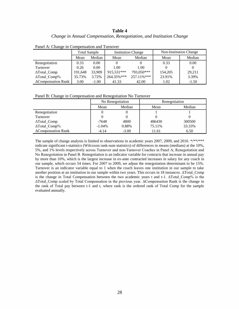
Table 4 reports changes in compensation for our sample and several sub-groups.
Examining coaches that remain in their current employment, a common research design choice
used by researchers when examining CEO total incentives, we find the mean (median) actual
change in year-to-year compensation to be 24% (3%), which equates to a mean (median)
increase in salary of $154,205 ($29,210). However, this mean change masks significant variation
in compensation changes across these coaches. As shown in Table 4 Panel B, coaches who
renegotiate their existing contract experience a mean (median) actual change in compensation of
75% (33%) compared to a mean (median) change of -1% (1%) for those that do not renegotiate.
Coaches that renegotiate their existing employment terms increase their mean (median)
compensation by $486,430 ($300,500) and increase their pay ranking in the NCAA head coach
labor market by 12 (7) mean (median) places.

14
4.2.2 Change in annual compensation due to institution change
An important advantage of the football coaches labor market over more commonly
investigated settings, such as CEOs, is the observation of agents’ employment outcomes after
their current employment. This limitation of other labor market settings almost always requires
researchers to deliberately exclude agents that leave their current employment in the following
year. For example, when investigating CEO pay-for-performance relations, CEOs that leave their
current employment due to being fired, hired at another firm or retired are removed from the
sample. This common research design choice that is driven by lack of data availability could
substantially distort the true relation between pay and performance.
We observe coaches changing institutions 20% of the time for 84 turnovers. Of the 84
turnovers in our sample, the coach moves to another institution in our sample within 1 season in
9 cases and moves to another institution within our sample in another 9 cases. In 14 cases, the
coach leaves their existing institution to join an organization in the National Football League. In
the remaining cases, the coach is either out of the market, or it takes longer than two years before
landing a coaching job at another FBS institution.
Table 4 Panel B shows that when coaches that change institutions to another head coach
position in our sample within two years they experience a mean (median) actual change in
compensation of 264% (257%), which equates to an increase in salary of $915,000 ($793,050)
and an increase in salary rank in the labor market by 41 (42) places.
Together, the results in changes in pay and turnovers support the conjecture that the labor
market is a strong source of incentives. That is, large increases in pay exist when coaches move
institutions. These findings demonstrate that in a labor market setting with a non-trivial
likelihood of external hiring and/or termination of employment the common research design

15
choice of excluding agents that do not remain in the same organization in consecutive years
substantially understates the true relation between pay-for-performance. Therefore, research that
does not consider how these sample choices distort the observed pay-for-performance may
substantially under-report the true convexity from total incentives. Overall, we find substantial
differences in compensation driven by successful head coaches either accepting new
employment or renegotiating their existing employment contract on better terms, which occurs
26% and 33% on average each coach-year, respectively. We explore the likelihood of these
outcomes in the following section.
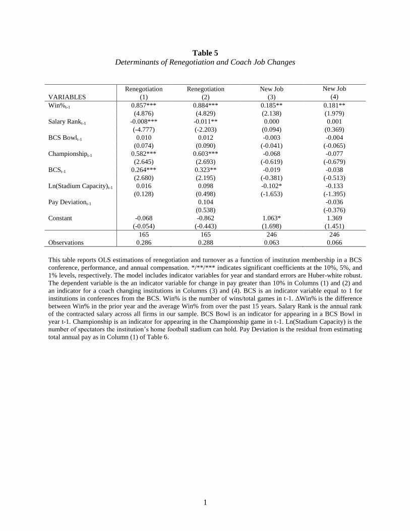
4.3 Likelihood of higher paid employment and renegotiation
We model both the likelihood of a head coach movement to higher paid employment or
renegotiating their existing employment contract on better terms as a function of the coach’s
team performance and college characteristics. Table 5 shows that the likelihood of renegotiation
is more likely when the coaches’ team has a higher winning percentage or appears in the national
championship game in the previous year. This evidence is consistent with Gibbons and Murphy
(1992: 470) conjecture that renegotiation mimics one of the effects of labor market competition.
We also find that likelihood of renegotiation is increasing in the size of the college, as
represented by the college being in a BCS conference and having a lower salary rank. This
evidence is consistent with renegotiation being more likely when the college has limited
competitors for the coach’s talent. At the same time, renegotiation is negatively related with the
salary rank. This suggests there is a ceiling in the market for coaches, where coaches at the
highest pay scale do not renegotiate their contracts even after strong performance.
Table 5 column 3 shows that the likelihood of higher paid employment (institution
change) is also significantly more likely when the coaches’ team performs well (higher winning
16
percentage in the previous year). However, the likelihood of institution change decreases with
college size (stadium capacity). Taken together, this suggests separating equilibrium across the
labor market where relatively smaller colleges are less able or willing to increase pay sufficiently
(renegotiate) to retain better performing coaches; and consequently, better performing coaches
leave for higher paying jobs in colleges that have greater capacity to pay. This suggests that
better performing coaches are more likely to leave current employment if there are more external
labor market opportunities to improve their employment terms. Overall, our results show how
implicit incentives become reflected in agent compensation – either within the firm or through
the external labor market – is dependent on the agent’s firm characteristics in the market for their
labor.
4.3.1 Alternative explanations
We examine three alternative explanations to this small college/large college equilibrium
pay story: 1) that departing coaches are lesser paid in their original employment; 2) that new
colleges overpay for head coaches from other colleges; and 3) that the original colleges would
have provided this pay increase.
First, we calculate the deviation in the coach’s salary from a model of expected total
compensation. Specifically, we estimate expected compensation for the coach in the year before
renegotiation or institution change, to determine if the coach’s action was in part due to being
relatively under paid in their original employment.
Table 6 Model 1 presents results from estimating expected compensation as a function of
performance in the prior year and college characteristics. Consistent with the univariate statistics,
we find total compensation is greater for college coaches in BCS conferences, coaches of
colleges with greater stadium capacity and those coaches that have a higher winning percentage
17
in recent years. The coefficient of 0.629 suggests that coaches of BCS teams earn $293,000 more
in annual compensation than coaches of teams that are non-AQ. Turning to performance, we find
that overall winning percentage is positively related to annual pay. Inspecting the coefficients
indicates that winning one more game in the regular season, which increases the winning
percentage by about 10% for a 10-game season is related to an increase in pay of $238,000, on
average. However, other measures of performance including bowl appearances and wins do not
relate to compensation levels. The overall explanatory power of our expectation model of total
compensation is reasonable, with an r-squared of 0.73.
We calculate the deviation in the coach’s salary from the Table 6 Model 1 of coaches
expected total compensation in the previous year to determine if it influences their career
outcomes. Examining the estimates from Table 5 column 2 and 4 we find no support that the
likelihood of renegotiation or institution change increases in the deviation from the expected
salary, suggesting that departing coaches are no lesser or better paid on average.
A second alternative to the separating equilibrium pay explanation is that colleges
overpay new coaches relative to optimal to entice them to leave their existing employment. To
test this explanation, in Column (2) we include an indicator for coach turnovers as an additional
covariate in the total compensation model. Specifically, if the coefficient on turnover is positive,
controlling for college characteristics and performance, this would suggest that colleges pay new
coaches greater than their expected pay to entice the coach to leave their original employment.
Examining the estimated coefficient for turnover, while the results found in Column (1) remain,
there is not a significant relation between annual pay and turnovers, This results suggests that
colleges compensate their coaches based on the economic determinants in a consistent manner
regardless of the stability of the coaching position.

18
A third alternative is that the increase in pay associated with turnover was likely to occur
regardless of the institution change, as the original institution would have ex-post settled up the
coach by paying a higher salary in future periods. To explore the relevance of this explanation
we model the change in coaches compensation as a function of the coach’s team’s recent
performance and college characteristics. If turnover, in and of itself, is not an important
determinant of change in coach pay we should not find an association between turnover and pay
change after controlling for recent performance. The results of this analysis are presented in
Table 6 column 3. Consistent with the univariate change in compensation, column 3 shows that
after controlling for the recent performance of the coach’s team, coaches that change institutions
experience a substantial increase in compensation. Therefore, we conclude our evidence is
consistent with large explicit incentives in the labor market for well-performing coaches.
5. Extensions
5.1 Explicit incentives
Our primary measure of explicit incentives is the maximum potential bonus divided by
annual salaried compensation. Obviously, it is infeasible for all coaches in our sample to receive
their maximum potential bonus, as most incentive bonuses are conditional on on-field
performance, such as winning games or championships. We selected this maximum bonus
measure to provide an upper bound of the importance of ex-ante explicit incentives, thereby
ensuring that our finding of explicit incentives being of limited importance was not driven by our
choice of estimating the likelihood of achieving various explicit bonuses. Therefore, while we
observe explicit incentives explain a small fraction of the total incentives, the expected explicit
component of total incentives is likely to be substantially smaller than reported.
19
In unreported results, we consider two alternative explicit incentive measures. First, we
consider an expectation model where all teams have an equal chance of winning every football
game, with all remaining unobservable off-field performance recorded at its maximum potential
bonus. Second, we consider an expectation model where teams’ likelihood of winning is based
on their historical performance over the previous 20 years. In unreported tests, all the cross-
sectional findings are invariant to using the alternative explicit incentive measures discussed
above.
5.2 Time horizon
Our main empirical results report the change in head coaches’ compensation in the year
following observed performance. Given the change in compensation observed is primarily driven
by the variation in coaches’ annual salaries – due to renegotiation or better employment – the
implications of the change in compensation is not limited to the following year. Rather, the
observed change influences all future year’s compensation both contractually and in expectation
(Gibbons and Murphy, 1992: 470). Therefore, the relative importance of implicit incentives is
likely to be greater than reported in this study. Future analysis can incorporate empirical
expectations of the likelihood of renegotiation, better employment, remaining on the existing
employment terms and involuntary termination with the distribution of expected compensation
for each of these job outcomes.
6. Conclusion
We provide novel evidence of the importance of explicit and implicit incentives in
contracting. We find that explicit pay-for-performance is of limited importance in the presence of
strong external implicit labor market incentives. Using the empirical advantages of the labor

20
market for NCAA head football coaches, we capture significant variation in agent compensation
and incentives not previously observed in pay-for-performance research. Specifically, by
observing agents’ renegotiation following good performance and their career outcomes after
current employment, we document substantial convexity in the pay-for-performance relation
driven predominantly by implicit incentives.
Our findings provide insight on a fundamental question of labor contracting in the
presence of external labor market incentives excluding internal promotion opportunities.
Obviously, the relative importance of ex-ante explicit incentives and ex-post settling up through
contract renegotiation will vary across labor markets conditional on many factors, including the
observability and noise of performance, transferability of human capital and the convexity in the
distribution of labor market compensation. Therefore, in settings where performance
observability is low and noise greater, there is limited transferable (greater institutional specific)
human capital and minimal pay convexity in the labor market, the importance of implicit
incentives should be reduced. In this regard, our evidence provides bounds for other labor
markets with no internal promotion opportunities, such as CEOs, where data availability inhibit
empirical investigation of labor market contracting. Overall, we demonstrate that in the presence
of strong external incentives and renegotiation that limited explicit pay-for-performance can
optimally incentivize workers.

21
References:
Boschen, J. F. and Smith, K. J. 1995. You can pay me now and you can pay me later: The
dynamic response of executive compensation to firm performance. Journal of Business
68(4): 577-608.
Brickley, J. A., Linck, J. S., and Coles, J. L. 1999. What happens to CEOs after they retire? New
evidence on career concerns, horizon problems, and CEO incentives. Journal of Financial
Economics 52(3): 341-377.
Chang, Y. Y., Dasgupta, S., and Hilary, G. 2010. CEO ability, pay, and firm performance.
Management Science 56(10): 1633-1652.
Ederhof, M. 2011. Incentive compensation and promotion-based incentives of mid-level
managers: Evidence from a multinational corporation. The Accounting Review 86(1): 131-
153.
Fama, E. F. 1980. Agency problems and the theory of the firm. Journal of Political Economy
88(2): 288-307.
Fee, C. E. and Hadlock, C. J. 2004. Management turnover across the corporate hierarchy.
Journal of Accounting and Economics 37(1): 3-38.
Fee, C. E., Hadlock, C. J., and Pierce, J. R. 2006. Promotions in the internal and external labor
market: Evidence from professional football coaching careers. Journal of Business 79(2):
821-850.
Gibbons, R. 2005. Incentives between firms (and within). Management Science 51(1): 2-17.
Gibbons, R. and Murphy, K. T. 1992. Optimal incentive contracts in the presence of career
concerns: Theory and evidence. Journal of Political Economy 100(3): 468-505.
Gillan, S. L., Hartzell, J. C., and Parrino, R. 2009. Explicit versus implicit contracts: Evidence
from CEO employment agreements. Journal of Finance 64(4): 1629-1655.
Hall, B. J. and Liebman, J. B. 1998. Are CEOs really paid like bureaucrats? Quarterly Journal of
Economics 113(3): 653-691.
Holmes, P. 2011. Win or go home: Why college football coaches get fired. Journal of Sports
Economics 12(2): 157-178.
Holmstrom, B. 1982. Managerial incentives schemes—a dynamic perspective. In Essays in
Economics and Management in Honor of Lars Wahlbeck. Helsinki: Swenska
Handelsho¨gkolan.
22
Inoue, Y., Plehn-Dujowich, J. M., Kent, A. and Swanson, S. 2012. Roles of performance and
human capital in college football coaches’ compensation. Journal of Sports Management
27(1): 73-83.
Kahn, L. M. 2000. The sports business as a labor market laboratory. Journal of Economic
Perspectives 14(3): 75-94.
Kahn, L. M. 2007. Markets: Cartel behavior and amateurism in college sports. Journal of
Economic Perspectives 21(1): 209-226.
Oyer, P. 2004, Why do firms use incentives that have no incentive effects? Journal of Finance
59(4): 1619–1649.
Parrino, R. 1997. CEO turnover and outside succession: A cross-sectional analysis. Journal of
Financial Economics 46(2): 165-197.
Rajgopal, S., Shevlin, T. and Zamora, V. 2006. CEOs’ outside employment opportunities and the
lack of relative performance evaluation in compensation contracts. Journal of Finance 61(4):
1813-1844.
23
Figure 1
Salary and Maximum Potential Bonus in 2010
0
1
2
3
4
5
6
7
$M
illi
on
s
Rank by Salary
Max Bonus
Salary
24
Table 1
Summary Compensation
Panel A: Summary Compensation-Full Sample
Year
University Salary Non-University Salary Potential Bonus
Total
Annual
Payment
University
Salary
% of Total Non-
University
Salary
% of Total Maximum
Total
Bonus
% of Total Total Pay
2006 475,201 66.16% 446,065 42.53% 236,245 27.66% 906,666
(300,000) (67.39%) (191,400) (37.19%) (162,400) (21.59%) (800,000)
2007 489,923 58.67% 627,480 47.68% 313,653 37.20% 1,041,685
(305,068) (58.57%) (337,500) (41.43%) (257,500) (28.23%) (930,325)
2009 595,529 57.36% 747,516 47.31% 447,894 41.53% 1,271,246
(375,000) (50.86%) (397,250) (53.13%) (392,750) (33.44%) (989,644)
2010 1,331,789 97.64% 34,596 2.36% 423,520 38.68% 1,366,385
(1,100,000) (99.86%) (1,000) (0.14%) (320,427) (34.09%) (1,101,500)
Total 724,794 70.00% 454,832 34.52% 354,983 36.12% 1,148,130
(400,405) (82.96%) (80,961) (17.86%) (274,048) (28.95%) (937,950)
Panel B: Summary Compensation by Conference in the BCS
Conference
University Salary Non-University Salary Potential Bonus
Total
Annual
Payment
University
Salary
% of Total Non-
University
Salary
% of Total Maximum
Total
Bonus
% of Total Total Pay
ACC 872,223 57.69% 904,821 57.89% 460,864 28.22% 1,586,782
(511,243) (48.15%) (533,425) (46.69%) (407,500) (23.79%) (1,726,103)
Big 10 1,117,064 67.46% 520,143 33.40% 450,425 32.65% 1,623,870
(760,000) (60.00%) (363,195) (40.00%) (375,000) (24.26%) (1,454,619)
Big 12 1,063,868 54.62% 803,180 44.96% 551,987 35.14% 1,874,861
(911,073) (38.38%) (687,500) (61.62%) (486,875) (26.98%) (1,720,784)
Big East 870,928 69.57% 387,031 32.59% 375,585 32.19% 1,235,837
(810,000) (67.50%) (347,966) (33.34%) (392,500) (29.20%) (1,101,500)
PAC-10 976,141 72.40% 491,734 53.66% 628,015 57.61% 1,434,453
(600,000) (51.98%) (397,488) (50.07%) (402,500) (41.58%) (1,275,000)
SEC 996,681 43.89% 1,137,476 57.39% 551,212 26.71% 2,128,975
(406,000) (26.44%) (954,000) (74.44%) (545,000) (20.20%) (2,028,100)
Total 990,621 59.76% 741,345 47.46% 509,582 35.02% 1,687,300
(638,441) (47.98%) (550,000) (53.13%) (452,000) (28.10%) (1,520,450)

25
Panel C: Summary Compensation by Conference in the non-AQ
Conference University Salary Non-University Salary Potential Bonus
Total
Annual Pay
University
Salary
% of Total Non-
University
Salary
% of Total Maximum
Total
Bonus
% of Total Total Pay
CUSA 507,172 71.54% 232,325 29.96% 238,173 35.57% 721,758
(379,000) (85.68%) (64,400) (16.70%) (232,167) (34.55%) (560,060)
Independent 630,668 88.89% 57,143 14.29% 250,000 62.50% 675,113
(640,851) (100.00%) (0) (0.00%) (225,000) (56.25%) (640,851)
MAC 243,315 89.07% 33,032 11.16% 162,207 58.12% 275,673
(200,850) (95.23%) (12,250) (5.70%) (140,000) (52.75%) (269,062)
MWC 599,681 75.18% 188,175 27.53% 270,209 36.69% 772,264
(500,000) (97.51%) (75,000) (15.96%) (171,625) (31.23%) (700,000)
Sun Belt 248,183 89.26% 26,837 11.06% 56,998 20.82% 274,254
(225,750) (96.23%) (8,650) (3.81%) (50,000) (18.75%) (261,000)
WAC 474,375 81.60% 100,707 18.92% 140,950 25.94% 572,285
(371,546) (90.43%) (46,810) (9.71%) (110,000) (15.85%) (390,663)
Total 409,293 82.16% 108,000 18.86% 171,135 37.44% 511,421
(305,822) (95.27%) (23,250) (8.77%) (125,000) (29.57%) (390,603)
The sample consists of …
University Salary is the Annual compensation paid by the University, Non-University Salary includes compensation
paid by corporate sponsors, media, and other organizations that are involved with the University and pay a portion
of the coache’s salary directly. Potential Bonus is the maximum bonus the coach can earn in a year for achieving
performance goals such as winning percentage, conference championships, bowl appearance, and national rankings.
Total Annual Pay is the sum of University and Non-University Salary. Panel A includes all teams in our sample
separated by academic year. Panel B reports summary statistics for each conference included in the Bowl
Championship Series. Panel C reports summary statistics for universities in conferences that are not automatic
qualifiers, but remain in the Football Championship Series (FBS).
26
Table 2
Performance Summary Statistics
Total Sample BCS Non-AQ
Mean Median Mean Median Mean Median
Win %t 51.85% 53.85% 56.96% 61.54% 45.11% 51.85%
Conference Win %t 47.09% 50.00% 46.71% 50.00% 47.64% 47.09%
Bowl Appearancet 0.58 1.00 0.70 1.00 0.43 0.58
BCS Bowl Appearancet 0.07 0.00 0.11 0.00 0.03 0.07
Bowl Wint 0.29 0.00 0.34 0.00 0.24 0.29
BCS is an indicator variable equal to 1 for institutions in conferences from the BCS, Non-AQ includes the
remaining firms that are in non-automatic qualifying conferences. Win% is the number of wins/total games
in academic year t. Conference Win% is the number of conference wins/total conference games in
academic year t. Bowl Appearance is an indicator for appearing in a post-season Bowl game in year t. BCS
Bowl Appearance is an indicator for appearing in one of the 4 premier BCS bowl games in year t. Bowl
Win is an indicator variable for winning a bowl game in year t-1.

27
Table 3
Determinants of Explicit Incentives as Measured by Bonus
Bonus% Bonus% Bonus%
VARIABLES (1) (2) (3)
Bowl Wint-1 0.005 0.005 0.007
(0.125) (0.110) (0.159)
Win%t-1 -0.261*** -0.136 -0.138
(-2.637) (-1.371) (-1.396)
Championshipt-1 -0.113 -0.068 -0.095
(-0.753) (-0.464) (-0.653)
BCS Bowlt-1 -0.040 -0.014 -0.015
(-0.494) (-0.182) (-0.186)
Ln(Stadium Capacity)t -0.020 0.250*** 0.242***
(-0.328) (3.757) (3.710)
BCSt-1 0.022
(0.428)
Ln(Total Comp)t -0.187***
(-4.916)
Salary Rankt -0.005***
(-4.916)
Constant 0.615 0.168 -2.002***
(0.989) (0.372) (-2.996)
Observations 384 384 384
R-squared 0.057 0.081 0.082
This table reports OLS estimations of Bonus% as a function of institution membership in a BCS
conference, performance, and annual compensation. */**/*** indicates significant coefficients at the 10%,
5%, and 1% levels, respectively. The model includes indicator variables for year and standard errors are
Huber-white robust. The dependent variable is the maximum potential bonus scaled by the total annual pay
excluding bonus in year t. Ln(Stadium Capacity) is the number of spectators the institution’s home football
stadium can hold. BCS is an indicator variable equal to 1 for institutions in conferences from the BCS.
Bowl Win is an indicator variable for winning a bowl game in year t-1. Win% is the number of wins/total
games in t-1. Championship is an indicator for appearing in the Championship game in t-1. BCS Bowl is an
indicator for appearing in a BCS Bowl in year t-1. Ln(Total Comp) is the natural log of total salary in year
t. Salary Rank is the annual rank of the contracted salary across all firms in our sample.
28
Table 4
Change in Annual Compensation, Renegotiation, and Institution Change
Panel A: Change in Compensation and Turnover
Total Sample Institution Change Non-Institution Change
Mean Median Mean Median Mean Median
Renegotiation 0.33 0.00 0 0 0.33 0.00
Turnover 0.26 0.00 1.00 1.00 0 0
ΔTotal_Comp 191,648 33,909 915,531*** 793,050*** 154,205 29,211
ΔTotal_Comp% 35.73% 3.72% 264.35%*** 257.11%*** 23.91% 3.39%
ΔCompensation Rank 3.00 -1.00 41.33 42.00 1.02 -1.50
Panel B: Change in Compensation and Renegotiation No Turnover
No Renegotiation Renegotiation
Mean Median Mean Median
Renegotiation 0 0 1 1
Turnover 0 0 0 0
ΔTotal_Comp -7648 4800 486430 300500
ΔTotal_Comp% -1.04% 0.88% 75.11% 33.33%
ΔCompensation Rank -4.14 -3.00 11.61 6.50
The sample of change analysis is limited to observations in academic years 2007, 2009, and 2010. */**/***
indicate significant t-statistics (Wilcoxon rank-sum statistics) of differences in means (medians) at the 10%,
5%, and 1% levels respectively across Turnover and non-Turnover Coaches in Panel A; Renegotiation and
No Renegotiation in Panel B. Renegotiation is an indicator variable for contracts that increase in annual pay
by more than 10%, which is the largest increase in ex-ante contracted increases in salary for any coach in
our sample, which occurs 54 times. For 2007 to 2009, we adjust the renegotiation determinant to be 15%.
Turnover is an indicator variable equal to 1 when the coach leaves one institution in our sample to take
another position at an institution in our sample within two years. This occurs in 18 instances. ΔTotal_Comp
is the change in Total Compensation between the two academic years t and t-1. ΔTotal_Comp% is the
ΔTotal_Comp scaled by Total Compensation in the previous year. ΔCompensation Rank is the change in
the rank of Total pay between t-1 and t, where rank is the ordered rank of Total Comp for the sample
evaluated annually.
1
Table 5
Determinants of Renegotiation and Coach Job Changes
Renegotiation Renegotiation New Job New Job
VARIABLES (1) (2) (3) (4)
Win%t-1 0.857*** 0.884*** 0.185** 0.181**
(4.876) (4.829) (2.138) (1.979)
Salary Rankt-1 -0.008*** -0.011** 0.000 0.001
(-4.777) (-2.203) (0.094) (0.369)
BCS Bowlt-1 0.010 0.012 -0.003 -0.004
(0.074) (0.090) (-0.041) (-0.065)
Championshipt-1 0.582*** 0.603*** -0.068 -0.077
(2.645) (2.693) (-0.619) (-0.679)
BCSt-1 0.264*** 0.323** -0.019 -0.038
(2.680) (2.195) (-0.381) (-0.513)
Ln(Stadium Capacity)t-1 0.016 0.098 -0.102* -0.133
(0.128) (0.498) (-1.653) (-1.395)
Pay Deviationt-1
0.104
-0.036
(0.538) (-0.376)
Constant -0.068 -0.862 1.063* 1.369
(-0.054) (-0.443) (1.698) (1.451)
165 165 246 246
Observations 0.286 0.288 0.063 0.066
This table reports OLS estimations of renegotiation and turnover as a function of institution membership in a BCS
conference, performance, and annual compensation. */**/*** indicates significant coefficients at the 10%, 5%, and
1% levels, respectively. The model includes indicator variables for year and standard errors are Huber-white robust.
The dependent variable is the an indicator variable for change in pay greater than 10% in Columns (1) and (2) and
an indicator for a coach changing institutions in Columns (3) and (4). BCS is an indicator variable equal to 1 for
institutions in conferences from the BCS. Win% is the number of wins/total games in t-1. ΔWin% is the difference
between Win% in the prior year and the average Win% from over the past 15 years. Salary Rank is the annual rank
of the contracted salary across all firms in our sample. BCS Bowl is an indicator for appearing in a BCS Bowl in
year t-1. Championship is an indicator for appearing in the Championship game in t-1. Ln(Stadium Capacity) is the
number of spectators the institution’s home football stadium can hold. Pay Deviation is the residual from estimating
total annual pay as in Column (1) of Table 6.

2
Table 6
Determinants of Total Compensation and the Effect of Changing Institutions
Total_Compt Total_Compt ΔLn(Total_Comp)t
VARIABLES (1) (2) (3)
Bowl Wint-1 0.028 -0.028 -0.131**
(0.540) (-0.487) (-2.296)
Win%t-1 0.627*** 0.606*** 0.382***
(5.348) (4.466) (2.654)
Championshipt-1 0.098 0.062 0.236
(0.602) (0.333) (1.326)
BCS Bowlt-1 0.115 0.190* 0.071
(1.239) (1.872) (0.699)
BCSt 0.629*** 0.657*** 0.040
(10.518) (9.740) (0.545)
Ln(Stadium Capacity)t 0.790*** 0.765*** -0.029
(11.131) (9.627) (-0.342)
Turnovert -0.045 1.011***
(-0.771) (8.761)
Constant 4.234*** 4.923*** 0.221
(5.762) (5.991) (0.250)
Observations 412 310 174
R-squared 0.728 0.733 0.394
This table reports OLS estimations of annual compensation as a function of institution membership in a BCS
conference, performance, and whether the coach recently moved to the institution. */**/*** indicates significant
coefficients at the 10%, 5%, and 1% levels, respectively. The model includes indicator variables for year and
standard errors are Huber-white robust. The dependent variable in Columns (1) and (2) is the Ln(Total Annual pay
(excluding bonus)) in year t. The dependent variable in Column (3) is the difference in the natural log of annual pay
for the coach in year t-1 and year t. If the coach changes institutions, the pay at the prior firm is included as Total
Compensation in t-1. Column (1) includes all observations in our sample, Column (2) is restricted to observations
after the first year of our sample, 2006 so that we can observe turnovers. Column (3) is limited to coaches that
remain in our sample for at least two years (regardless of the institution) so that the change in pay can be measured.
BCS is an indicator variable equal to 1 for institutions in conferences from the BCS. Bowl Win is an indicator
variable for winning a bowl game in year t-1. Win% is the number of wins/total games in t-1. Championship is an
indicator for appearing in the Championship game in t-1. BCS Bowl is an indicator for appearing in a BCS Bowl in
year t-1. Ln(Stadium Capacity) is the number of spectators the institution’s home football stadium can hold.
Turnover is an indicator for coaches that moved from one institution in our sample to another over the past year.