Explicit Adaptive Symplectic Integrators for solving ... · Explicit Adaptive Symplectic...
23
Celestial Mechanics and Dynamical Astronomy manuscript No. (will be inserted by the editor) Explicit Adaptive Symplectic Integrators for solving Hamiltonian Systems Sergio Blanes · Arieh Iserles Received: date / Accepted: date Abstract We consider Sundman and Poincar´ e transformations for the long-time numerical integration of Hamiltonian systems whose evolution occurs at different time scales. The transformed systems are numerically integrated using explicit symplectic methods. The schemes we consider are explicit symplectic methods with adaptive time steps and they generalise other methods from the literature, while exhibiting a high performance. The Sundman transformation can also be used on non-Hamiltonian systems while the Poincar´ e transformation can be used, in some cases, with more efficient symplectic integrators. The performance of both transformations with different symplectic methods is analysed on several numerical examples. Keywords Symplectic Integrators · Adaptive time step · Hamiltonian systems 1 Introduction We consider the long-time numerical integration of dynamical systems whose evo- lution is governed by the Hamiltonian function H = 1 2 p > p + V (q), (1) SB acknowledges the support of the Ministerio de Ciencia e Innovaci´on (Spain) under the coordinated project MTM2010-18246-C03 (co-financed by the ERDF of the European Union). Sergio Blanes Instituto de Matem´atica Multidisciplinar, Universitat Polit` ecnica de Valencia, E-46022 Valencia, Spain. E-mail: [email protected] Arieh Iserles DAMTP, Centre for Mathematical Sciences, University of Cambridge, Wilberforce Rd, Cambridge CB3 0WA, United Kingdom E-mail: [email protected]
Transcript of Explicit Adaptive Symplectic Integrators for solving ... · Explicit Adaptive Symplectic...

Celestial Mechanics and Dynamical Astronomy manuscript No.(will be inserted by the editor)
Explicit Adaptive Symplectic Integrators for solvingHamiltonian Systems
Sergio Blanes · Arieh Iserles
Received: date / Accepted: date
Abstract We consider Sundman and Poincare transformations for the long-timenumerical integration of Hamiltonian systems whose evolution occurs at differenttime scales. The transformed systems are numerically integrated using explicitsymplectic methods. The schemes we consider are explicit symplectic methodswith adaptive time steps and they generalise other methods from the literature,while exhibiting a high performance. The Sundman transformation can also beused on non-Hamiltonian systems while the Poincare transformation can be used,in some cases, with more efficient symplectic integrators. The performance of bothtransformations with different symplectic methods is analysed on several numericalexamples.
Keywords Symplectic Integrators · Adaptive time step · Hamiltonian systems
1 Introduction
We consider the long-time numerical integration of dynamical systems whose evo-lution is governed by the Hamiltonian function
H =1
2p>p + V (q), (1)
SB acknowledges the support of the Ministerio de Ciencia e Innovacion (Spain) under thecoordinated project MTM2010-18246-C03 (co-financed by the ERDF of the European Union).
Sergio BlanesInstituto de Matematica Multidisciplinar,Universitat Politecnica de Valencia, E-46022 Valencia, Spain.E-mail: [email protected]
Arieh IserlesDAMTP, Centre for Mathematical Sciences,University of Cambridge, Wilberforce Rd,Cambridge CB3 0WA, United KingdomE-mail: [email protected]

2 Sergio Blanes, Arieh Iserles
with q,p ∈ Rd, and such that the system evolves at different time scales. Effec-tive long-time numerical integration requires to use adaptive time steps, conse-quently we wish to implement symplectic methods with adaptive time steps. Tothis purpose, we consider both the Sundman and the Poincare transformations.The schemes proposed generalise other methods from the literature and allow usto build new explicit adaptive symplectic schemes exhibiting a high performance.
Numerical solution of Hamiltonian systems is frequently carried out by sym-plectic integrators (SIs) due to their good performance in moderate and long-time integration Hairer et al (2006); Iserles (2008); Leimkuhler and Reich (2004);McLachlan and Quispel (2002); Sanz-Serna and Calvo (1994). SIs belong to thefamily of Geometric Numerical Integrators (methods which preserve important qual-itative and geometric properties of the underlying differential system) and are ar-guably the most popular methods in this class. Certain qualitative properties ofthe evolution, like symplecticity, are preserved and, in general, they exhibit smallererror growth along the numerical trajectory.
Splitting methods applied to separable Hamiltonian systems are the most fre-quently used symplectic integrators. Denoting by ΦH
t the t-flow of the system,z(t) = ΦH
t (z(0)), with z = (q,p)>, the exact flow for one time step, h, can be ap-
proximated by a composition of the flows associated to the kinetic energy Φ[T ]h and
potential energy, Φ[V ]h . The second order V TV leap-frog/Stormer/Verlet method
is given by the composition
Ψh ≡ Φ[V ]
h/2 Φ
[T ]h Φ
[V ]
h/2:
pn+1/2 = pn − h
2∇qV (qn)
qn+1 = qn + hpn+1/2
pn+1 = pn+1/2 −h
2∇qV (qn+1)
. (2)
(Analogously, one can also take the TV T version.)More accurate results can be obtained by using higher order methods. Splitting
symplectic methods exist for a range of problems with different structure, lead-ing to high-performance numerical schemes. For instance, splitting Runge–Kutta–Nystrom (RKN) methods are tailored for Hamiltonian systems with quadratickinetic energy, and there are also splitting methods tailored for perturbed systemswhere the Hamiltonian takes the form
H = H0(p,q) + εHI(q) =
(1
2p>p + V0(q)
)+ εVI(q), (3)
where H0 is exactly solvable and 0 < |ε| ¿ 1, an important such case beingperturbed Kepler problems. We can then adapt the Verlet method (2) to thecomposition
Ψ[2]h ≡ Φ
[HI ]
h/2 Φ
[H0]h Φ
[HI ]
h/2= ΦH
h +O(εh3) (4)
to gain a factor ε in the accuracy Kinoshita et al (1991); Wisdom and Holman(1991).
A systematic procedure to build higher-order methods was introduced in Creutzand Gocksch (1989); Suzuki (1990); Yoshida (1990), and since then considerableeffort has been expanded in order to construct new symplectic integrators withsmaller local errors at a given computational cost. A significant number of newsplit symplectic integrators have been published for a wide number of problems
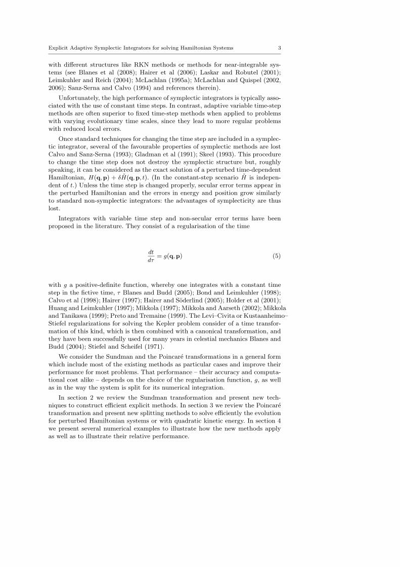
Explicit Adaptive Symplectic Integrators for solving Hamiltonian Systems 3
with different structures like RKN methods or methods for near-integrable sys-tems (see Blanes et al (2008); Hairer et al (2006); Laskar and Robutel (2001);Leimkuhler and Reich (2004); McLachlan (1995a); McLachlan and Quispel (2002,2006); Sanz-Serna and Calvo (1994) and references therein).
Unfortunately, the high performance of symplectic integrators is typically asso-ciated with the use of constant time steps. In contrast, adaptive variable time-stepmethods are often superior to fixed time-step methods when applied to problemswith varying evolutionary time scales, since they lead to more regular problemswith reduced local errors.
Once standard techniques for changing the time step are included in a symplec-tic integrator, several of the favourable properties of symplectic methods are lostCalvo and Sanz-Serna (1993); Gladman et al (1991); Skeel (1993). This procedureto change the time step does not destroy the symplectic structure but, roughlyspeaking, it can be considered as the exact solution of a perturbed time-dependentHamiltonian, H(q,p) + δH(q,p, t). (In the constant-step scenario H is indepen-dent of t.) Unless the time step is changed properly, secular error terms appear inthe perturbed Hamiltonian and the errors in energy and position grow similarlyto standard non-symplectic integrators: the advantages of symplecticity are thuslost.
Integrators with variable time step and non-secular error terms have beenproposed in the literature. They consist of a regularisation of the time
dt
dτ= g(q,p) (5)
with g a positive-definite function, whereby one integrates with a constant timestep in the fictive time, τ Blanes and Budd (2005); Bond and Leimkuhler (1998);Calvo et al (1998); Hairer (1997); Hairer and Soderlind (2005); Holder et al (2001);Huang and Leimkuhler (1997); Mikkola (1997); Mikkola and Aarseth (2002); Mikkolaand Tanikawa (1999); Preto and Tremaine (1999). The Levi–Civita or Kustaanheimo–Stiefel regularizations for solving the Kepler problem consider of a time transfor-mation of this kind, which is then combined with a canonical transformation, andthey have been successfully used for many years in celestial mechanics Blanes andBudd (2004); Stiefel and Scheifel (1971).
We consider the Sundman and the Poincare transformations in a general formwhich include most of the existing methods as particular cases and improve theirperformance for most problems. That performance – their accuracy and computa-tional cost alike – depends on the choice of the regularisation function, g, as wellas in the way the system is split for its numerical integration.
In section 2 we review the Sundman transformation and present new tech-niques to construct efficient explicit methods. In section 3 we review the Poincaretransformation and present new splitting methods to solve efficiently the evolutionfor perturbed Hamiltonian systems or with quadratic kinetic energy. In section 4we present several numerical examples to illustrate how the new methods applyas well as to illustrate their relative performance.

4 Sergio Blanes, Arieh Iserles
2 Explicit adaptive SIs using the Sundman transformation
The Sundman transformation takes the real time as a new coordinate and intro-duces a fictitious time, τ in the following manner,
d
dτ
q
p
t
=
g(q,p)p−g(q,p)∇V (q)
g(q,p)
. (6)
This equation loses the symplectic structure and, in addition, most explicit meth-ods available in the literature for the numerical integration of the Hamiltonian (1)cannot be used or are highly inefficient in this setting. It has been shown, how-ever, that if a reversible time-symmetric method is used, many good propertiesfor long-time integrations are retained. Note that if the regularisation function g
is frozen at each step (or at each stage inside a step) then we can use an explicitsymplectic integrator and the coordinates (q,p) will evolve through a symplectictransformation. Thus, it is only necessary to look for an appropriate procedure tofreeze the function g in a manner which renders the whole numerical integration re-versible and time-symmetric, leading to an adaptive symplectic and time-reversibleintegrator.
We introduce an auxiliary scalar variable, z, and a positive-definite and in-vertible function, G(z), such that G(z) = g(z). To avoid some instabilities, wedifferentiate this equation so, the system to be solved is
d
dτ
q
p
t
z
=
G(z)p−G(z)∇V (q)
G(z)(G(g(q,p))−1
)′G(z)
(∇g(q,p) · f
)
(7)
where f ≡ J∇H(q,p) and J denotes the standard (2d)× (2d) symplectic matrix.Numerical integration of this problem has been considered in the literature for
different choices of the function G(z), the monitor function, g(q,p) and by splittingthe system in different ways. Since G(z)/g(q,p) = 1 is a first integral of the system,it has been usual to substitute G(z) by g(q,p) in different places on the right-handside of the equation, and in particular in the equation for dz/dτ . For example,Huang and Leimkuhler (1997); Leimkuhler and Reich (2004) employs the choiceG(z) = z while Hairer and Soderlind (2005); Mikkola and Aarseth (2002) (see also(Hairer et al, 2006, Sec. VIII.3.2)) use G(z) = 1/z. These are two particular casesof the more general function G(z) = zα, where the choice α = 0 corresponds to noregularisation. As we will see, the choice of G(z) plays an important role in theperformance of the algorithm.
The monitor function g is also very important in constructing efficient algo-rithms Blanes and Budd (2005). For the system (1), fast evolutions usually occurclose to the singularities of the potential. Thus, it makes sense to consider a func-tion depending only on the coordinates, say, g(q). However, other choices are alsovalid and the main differences impacts on the complexity when computing theequation for z′ (where the prime denotes the derivative with respect to τ).
Finally, one has to decide how to split the system in order to use a time-symmetric splitting method which preserves symplecticity for the coordinates q,p.For example, in Hairer and Soderlind (2005) (see also (Hairer et al, 2006, Sec.

Explicit Adaptive Symplectic Integrators for solving Hamiltonian Systems 5
VIII.3.2)), where G(z) = 1/z, g(q) = (q>q)γ (for problems where the singularityof the potential is at the origin), the function G(z) is replaced by g(q) in theequation of z′, and the system is split as follows
d
dτ
q
p
t
z
=
1
zp
−1
z∇V (q)
1
z0
︸ ︷︷ ︸fA
+
0
0
0
−γq>p
q>q
︸ ︷︷ ︸fB
. (8)
The system is then solved using the composition
Ψh = Φ(B)
h/2 Φ
(A)h Φ
(B)
h/2(9)
with h ≡ δτ . Here, Φ(B)
h/2is used only to change the time step for the real time.
Consequently, one can replace Φ(A)h by the desired symplectic integrator to advance
q,p and t. This is a second-order approximation in the auxiliary variable z, whichis not relevant to the accuracy of the method. The practical order of accuracy
follows from the order of the method used to approximate Φ(A)h .
This is a simple time-reversible explicit symplectic integrator and it is perhapsthe most efficient algorithm for low to moderate accuracies. However, if accurateresults are desired, high-order methods are necessary. High-order methods usuallyrequire many evaluations per step and demonstrate their superior performancewhen relatively large time steps are used in lieu of the extra per-step cost. However,
this scheme changes the time step only when the flow Φ(B)h is computed, hence to
use a relatively large time step can be dangerous when the system moves close tothe singularities because the scheme has no opportunity to adapt the time step.
We then propose to split the system as follows,
d
dτ
q
p
t
z
=
G(z)p0
G(z)0
︸ ︷︷ ︸fA
+
0
0
0(G(g)−1
)′G(z)(∇g · f)
︸ ︷︷ ︸fB
+
0
−G(z)∇V
00
︸ ︷︷ ︸fC
. (10)
The right hand side of the equation for dt/dτ could be put into any of the threevector fields and each part would be still exactly solvable but it is advantageousto keep it in either fA or fC .
We propose to use the following symmetric second order composition
S[2]h = Φ
(A)
h/2 Φ
(B)
h/2 Φ
(C)h Φ
(B)
h/2 Φ
(A)
h/2. (11)
Other sequences of the maps are also valid. Next, to reach high accuracy one canuse this method as the basic method to build higher order methods by composition,i.e.
S[2p]h = S
[2]αmh · · · S
[2]α1h

6 Sergio Blanes, Arieh Iserles
where the coefficients αi are chosen appropriately to build efficient methods oforder 2p in the time step h Hairer et al (2006); McLachlan (1995b); McLachlan andQuispel (2002); Sophroniou and Spaletta (2005). Notice that in this approach thetime step is adjusted along the internal stages of the method instead of adjustingthe time step by the end of the step.
Constructing methods of order four or six, it is usually more efficient to consider
a composition of a first order method, say, Φh = Φ(A)h Φ
(B)h Φ
(C)h and its adjoint
Φ∗h = Φ(C)h Φ
(B)h Φ
(A)h in an appropriate sequence Blanes and Moan (2002).
The choice of the monitor function We have to remark that the choice of the monitorfunction g is essential in constructing efficient methods Blanes and Budd (2005);Budd et al (2001); Calvo et al (1998); Hairer (1997); Hairer et al (2006). Thenumerical accuracy of a given scheme can be similar for different choices of g whileits computational cost can change drastically. Then, one has to choose the mostappropriate monitor function which must also satisfy the required conditions (e.g.preserving scaling invariance of the system or any reversing symmetry) and thishas to be done in tandem with the choice of the function G(z) in order to obtainsimple and easy to compute expression for z′. For example, if the potential functionis given by V (r) with r = (q>q)1/2 then it seems appropriate to choose g = g(r)because then, replacing G(z) by g(r), the equation for z′ becomes z′ = F (r)(q>p),with F (r) a given scalar function. Another important property to be analysedis how the choice of the function G(z) affects the performance of the numericalmethods.
To sum up, the Sundman transformation allows us to build explicit time re-versible adaptive integrators to high order. However, RKN methods or methodstailored for near integrable systems can not be used, unless the system is split asin (8), which has some limitations as previously mentioned. To circumvent thisproblem, we will consider the Poincare transformation.
2.1 Some other particular cases
The scheme that we have proposed generalises other schemes used to numericallysolve the system (6) which have appeared in the literature.
In Leimkuhler and Reich (2004) an algorithm (previously obtained in Huangand Leimkuhler (1997)) is presented which corresponds to G(z) = z, consideringz = g in the equation of z′, and employing the splitting
d
dτ
q
p
t
z
=
zp
0
z
0
︸ ︷︷ ︸fA
+
0
−z∇V
0g(∇g · f)
︸ ︷︷ ︸fB
(12)
where we let g(q,p) = ‖f‖. With this splitting and the choice of g, the finalalgorithm has to be necessarily implicit. In Leimkuhler and Reich (2004) the h-flow ΦB
h is approximated by the first order explicit Euler method, ΦBh , and its

Explicit Adaptive Symplectic Integrators for solving Hamiltonian Systems 7
implicit adjoint method, Φ∗Bh , and constructs the following implicit symmetricsecond order method
Sh = ΦBh/2 ΦA
h Φ∗Bh/2. (13)
This method requires the computation of the Hessian of the potential and for thisreason it can be computationally costly for many problems.
In Mikkola and Aarseth (2002), the authors consider a monitor function de-pending only on the coordinates, g(q), let G(z) = 1/z (although the method ispresented in terms of the function Ω(q) = 1/g(q)) so that z′ = −(∇qg · p)/g andthe algorithm proposed is basically equivalent to considering the splitting
d
dτ
q
p
t
z
=
1
zp
01
z0
︸ ︷︷ ︸fA
+
0
−g∇V
0
−1
g(∇qg · p)
︸ ︷︷ ︸fB
. (14)
Note that the equation for fB is exactly solvable because the equation for z′ is linearin p. With this splitting, in Mikkola and Aarseth (2002) the authors construct thescheme
Sh = ΦAh/2 ΦB
h ΦAh/2 (15)
which is then taken as the basic method to be used with the Gragg–Bulirsch–Stoerextrapolation method. However, an extrapolation method based on a symmet-ric second order symplectic integrator is not appropriate because it loses sym-plecticity and its benefits for long-time integration. One can obtain, however,pseudo-symplectic integrators by extrapolation if the basic method is of higherorder Blanes et al (1999); Chan and Murua (2000) and qualitative properties arepreserved up to higher order than the order of the method. We recommend hisprocedure only when high accuracy is desired, say, to nearly round-off level andrelatively short time integrations.
Alternatively, one can solve the system (14) by standard splitting methods forseparable systems. Here, both q and p evolve through symplectic maps only ifg∇V is the gradient of a potential, and this deserves further investigation.
3 The Poincare transformation
Given a Hamiltonian H(q,p), the Poincare transformation introduces the followingnew Hamiltonian in the extended phase space,
H(q,p, qt, pt) = g(q,p)(H(q,p) + pt) (16)
where qt ≡ t and pt is its conjugate momentum. Note that H is autonomous,therefore H does not depend on qt, and pt is a constant of motion whose value isusually taken as pt = −H0 with H0 ≡ H(q(0),q(0)), consequently H = 0 along thesolution. The structure of the Hamiltonian H differs in general from the structureof H, i.e. if H is separable in solvable parts, in general, H will not be separable insolvable parts.
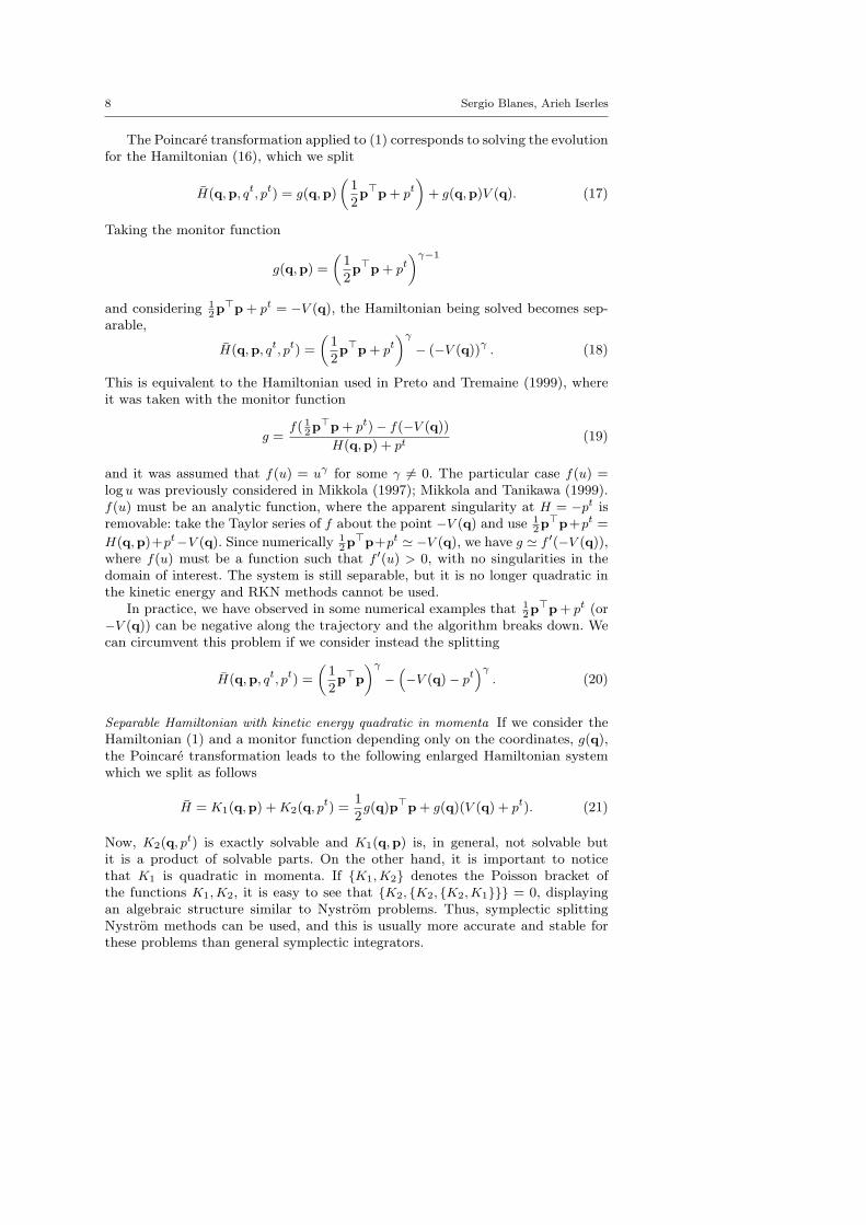
8 Sergio Blanes, Arieh Iserles
The Poincare transformation applied to (1) corresponds to solving the evolutionfor the Hamiltonian (16), which we split
H(q,p, qt, pt) = g(q,p)
(1
2p>p + pt
)+ g(q,p)V (q). (17)
Taking the monitor function
g(q,p) =
(1
2p>p + pt
)γ−1
and considering 12p>p + pt = −V (q), the Hamiltonian being solved becomes sep-
arable,
H(q,p, qt, pt) =
(1
2p>p + pt
)γ
− (−V (q))γ
. (18)
This is equivalent to the Hamiltonian used in Preto and Tremaine (1999), whereit was taken with the monitor function
g =f(1
2p>p + pt)− f(−V (q))
H(q,p) + pt(19)
and it was assumed that f(u) = uγ for some γ 6= 0. The particular case f(u) =log u was previously considered in Mikkola (1997); Mikkola and Tanikawa (1999).f(u) must be an analytic function, where the apparent singularity at H = −pt isremovable: take the Taylor series of f about the point −V (q) and use 1
2p>p+pt =
H(q,p)+pt−V (q). Since numerically 12p>p+pt ' −V (q), we have g ' f ′(−V (q)),
where f(u) must be a function such that f ′(u) > 0, with no singularities in thedomain of interest. The system is still separable, but it is no longer quadratic inthe kinetic energy and RKN methods cannot be used.
In practice, we have observed in some numerical examples that 12p>p + pt (or
−V (q)) can be negative along the trajectory and the algorithm breaks down. Wecan circumvent this problem if we consider instead the splitting
H(q,p, qt, pt) =
(1
2p>p
)γ
−(−V (q)− pt
)γ. (20)
Separable Hamiltonian with kinetic energy quadratic in momenta If we consider theHamiltonian (1) and a monitor function depending only on the coordinates, g(q),the Poincare transformation leads to the following enlarged Hamiltonian systemwhich we split as follows
H = K1(q,p) + K2(q, pt) =1
2g(q)p>p + g(q)(V (q) + pt). (21)
Now, K2(q, pt) is exactly solvable and K1(q,p) is, in general, not solvable butit is a product of solvable parts. On the other hand, it is important to noticethat K1 is quadratic in momenta. If K1, K2 denotes the Poisson bracket ofthe functions K1, K2, it is easy to see that K2, K2, K2, K1 = 0, displayingan algebraic structure similar to Nystrom problems. Thus, symplectic splittingNystrom methods can be used, and this is usually more accurate and stable forthese problems than general symplectic integrators.

Explicit Adaptive Symplectic Integrators for solving Hamiltonian Systems 9
For this purpose, we need an algorithm to approximate efficiently and accu-rately the evolution for the Hamiltonian
K1 =1
2g(q)p>p.
In Blanes and Budd (2005) it is shown that in some cases one can find acanonical transformation, (q,p) → (Q,P) where q = Φ(Q), Φ′(Q)T p = q, suchthat K1 depends only on the new momenta. Unfortunately, this occurs rarelyand we look for an alternative procedure. This can be done in different ways,and the most appropriate one will depend on the particular problem. If g(q) ischeap to compute function e.g. the singularity of the potential involves only fewcontributions (i.e. if it involves only two bodies in a N-body problem) we cannumerically solve efficiently the equations for K1 to roundoff accuracy at eachstage.
For instance, we can use a logarithmic method. Notice that the evolution forone time step ∆τ of K1 = 1
2g(q)p>p is equivalent to the evolution for one timestep ∆δ = E1∆τ with E1 = K1 of the Hamiltonian
KL = KL,1 + KL,2 = log(g(q)) + log(p>p), (22)
(during this evolution K1 is kept constant) as is immediate to see from the Hamil-tonian equations. At near collisions, 1
2p>p and g take large and small values,respectively, but logarithmic functions reduce these large values and maintain theeffectiveness of the splitting. The Hamilton equations for KL,1 and KL,2 are:
dq
dτ= 0,
dp
dτ= −1
g∇qg,
dq
dτ= 2
p
p>p,
dp
dτ= 0.
(23)
In general, we can take g in a very simple form, just by considering the singularitiesof the potential. If the system is scaling invariant (or close to it) as happens formost practical potentials with singularities or strong interactions, the optimalregularisation function g is closely related with the choice which preserves thisscaling invariance Blanes and Budd (2004, 2005); Budd et al (2001). Then, if wetake
g = (q>q)γ/2 (24)
for an appropriate choice of γ, we have
1
g∇qg = γ
q
q>q
rendering both parts of (23) trivial to compute with simple and cheap arithmeticoperations, so the evolution for K1 can be easily computed to roundoff accuracywith marginal extra cost.
It is important to bear in mind that, solving K in (22), the value of E1 changesfrom one stage to the next for the entire method. As we have already mentioned,to change the Hamiltonian at each step from information originating in the previ-ous step introduces, in general, secular errors. To diminish these errors to nearlyroundoff, the system has to be numerically solved to a very high accuracy, so theseerrors can be sufficiently diminished for practical purposes. This can be achieved,e.g. using a high order composition.

10 Sergio Blanes, Arieh Iserles
A nearly-integrable Hamiltonian Let us now consider the perturbed Hamiltonian
H(q,p) = H0(q,p) + εH1(q), (25)
where H0 is exactly solvable and 0 < |ε| ¿ 1, but occasionally the perturbationcan approach a singularity and it can take large values. For this problem it isconvenient to split the Hamiltonian into the dominant part and the perturbationbecause the error of numerical methods reduces considerably, but we need to adaptthe time step when the perturbation is more relevant. This is the case, for instance,with the N-body problem in the solar system, where the Hamiltonian can be splitinto pure Kepler problems and weak interactions between planets. In some cases,however, close approaches between the planets or asteroids can occur and, in spiteof ε being a small parameter, the Hamiltonian H1(q) can be nearly singular. Inthis case it is convenient to introduce adaptivity.
There are two natural choices for the regularisation function: g(H0 + pt) andg(q). In the first case, the Hamiltonian to solve is (considering that H0+pt = −εH1)
H = g(H0 + pt)(H0 + pt) + εg(−εH1)H1. (26)
The Hamiltonian g(H0 + pt)(H0 + pt) exhibits the same difficulty as H0, and itis also exactly solvable. However, for the choice g(u)u = uγ we have found inseveral problems that H0+pt takes negative values. In that case, one can integrate,backward in time, the Hamiltonian, −H, in order to keep both parts positive.
The evolution of a Hamiltonian system is unaltered by adding an arbitraryconstant so, we can introduce a constant δ such that
εH1 + δ < 0,
consequently H0 + pt > 0, and the new Hamiltonian to consider is
H = g(H0 + pt)(H0 + pt)− g(−εH1 − δ)(−εH1 − δ), (27)
which has lost the structure of a perturbed system: the performance of the splittingmethods tailored for perturbed systems is then seriously degraded.
However, if we take e.g. g(q) = (q>q)γ , the Hamiltonian becomes
H = (q>q)γ(H0 + pt) + ε(q>q)γH1(q), (28)
which retains the near integrable structure, but we need to solve accurately andefficiently the Hamiltonian
K1 = (q>q)γ(H0 + pt). (29)
We can use the logarithmic method as previously, the main trouble being thatH0 + pt must be positive definite (if not, we can take K1 = −(q>q)γ(−H0 − pt)and integrate backward in time the Hamiltonian (q>q)γ(−H0 − pt)) and eachstage would need to evaluate the Hamiltonian H0 several times. If this part isnot computationally costly and the perturbation H1 is the most costly part of thealgorithm, this splitting might be useful because it benefits from the perturbedstructure. We conclude with an interesting open problem, efficient time-reversibleSIs for Hamiltonians of the form H = H1(q,p)H2(q,p), where H1 and H2 areexactly solvable Hamiltonian functions.

Explicit Adaptive Symplectic Integrators for solving Hamiltonian Systems 11
4 Numerical Examples
We consider the integration of several examples by considering both the Sundmanand the Poincare transformations jointly with appropriate splitting and composi-
tion methods. Given a symmetric second order (implicit or explicit) method, S[2]h ,
we consider m-stage symmetric compositions of order n as follows
Smn ≡ S[2]α1h S
[2]α2h · · ·S
[2]αkh S
[2]αk+1h S
[2]αkh · · ·S
[2]α2h S
[2]α1h
with m = 2k + 1. The following composition methods are chosen for that purpose
– S54: the 5-stage fourth-order composition,– S96: the 9-stage sixth-order composition,– S178: the 17-stage eighth-order composition,
and whose coefficients can be found in Hairer et al (2006). In Sophroniou andSpaletta (2005) more elaborated compositions with additional extra stages areobtained with slightly improved performance.
The following splitting methods are considered for problems where RKN meth-ods or methods for near-integrable systems can be used
– RKN64: the 6-stage fourth-order BAB method from Blanes and Moan (2002),– RKN116: the 11-stage sixth-order BAB method from Blanes and Moan (2002),– M84: the 5-stage (8,4) BAB method from McLachlan (1995a) for perturbed
systems.
4.1 The one-dimensional Kepler problem
Let us consider the Kepler problem, which possesses periodic orbits with closeapproaches. Such an orbit has a radial coordinate q with associated momentum p
which evolves according to the Hamiltonian
H =1
2p2 − 1
q+
ε
q2, (30)
where√
ε is the angular momentum. In numerical tests we take the initial condi-tions (q0, p0) = (1, 0) and ε = 0.001 (which allows for very close approaches).
We first study the performance of different algorithms when using the Sundmantransformation. We take G(z) = 1/z, integrate until t = 100 and measure theaverage relative error in energy when considering the splitting shown in (8)–(9)or when considering (10)–(11). In the first case, The compositions are used to
approximate Φ(A)h in (9) as composition of the leapfrog scheme as the basic method,
or they are used as compositions of the second-order scheme (11). The time step isadjusted in all cases such that the final time is reached using approximately 50000evaluations of the potential. Fig. 1 displays the results obtained when consideringthe regularisation function g = qγ for different values of γ. It is clear from theresults that adjusting the time step through the variable z along the internalstages of the method allows us to greatly improve the performance of the methodsonce high-order methods are used to reach high accuracy.
We next repeat the experiment for G(z) = zα and different values of α. Wemeasure the accuracy of S178 when the monitor function g = qγ is used with its
12 Sergio Blanes, Arieh Iserles
1.3 1.4 1.5 1.6 1.7−9
−8
−7
−6
−5
−4
−3
−2
γ
LOG
10(R
EL.
ER
RO
R)
S12
S54
S96
S178
1.3 1.4 1.5 1.6 1.7−9
−8
−7
−6
−5
−4
−3
−2
γ
LOG
10(R
EL.
ER
RO
R)
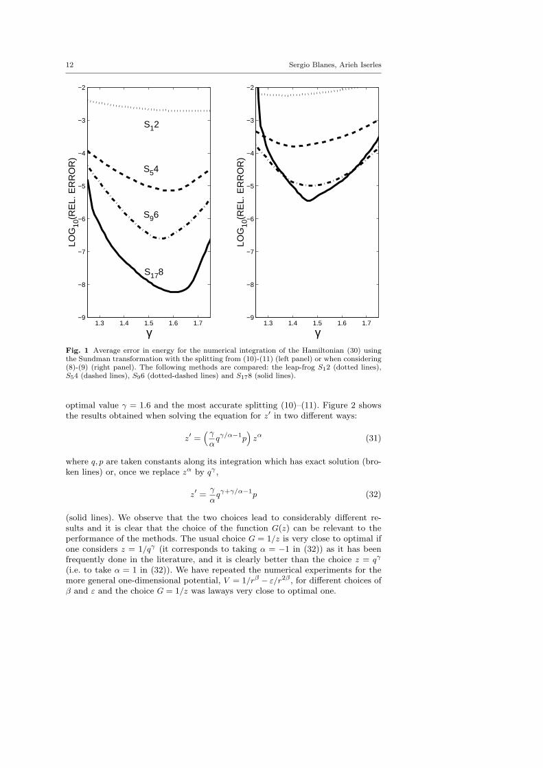
Fig. 1 Average error in energy for the numerical integration of the Hamiltonian (30) usingthe Sundman transformation with the splitting from (10)-(11) (left panel) or when considering(8)-(9) (right panel). The following methods are compared: the leap-frog S12 (dotted lines),S54 (dashed lines), S96 (dotted-dashed lines) and S178 (solid lines).
optimal value γ = 1.6 and the most accurate splitting (10)–(11). Figure 2 showsthe results obtained when solving the equation for z′ in two different ways:
z′ =( γ
αqγ/α−1p
)zα (31)
where q, p are taken constants along its integration which has exact solution (bro-ken lines) or, once we replace zα by qγ ,
z′ = γ
αqγ+γ/α−1p (32)
(solid lines). We observe that the two choices lead to considerably different re-sults and it is clear that the choice of the function G(z) can be relevant to theperformance of the methods. The usual choice G = 1/z is very close to optimal ifone considers z = 1/qγ (it corresponds to taking α = −1 in (32)) as it has beenfrequently done in the literature, and it is clearly better than the choice z = qγ
(i.e. to take α = 1 in (32)). We have repeated the numerical experiments for themore general one-dimensional potential, V = 1/rβ − ε/r2β , for different choices ofβ and ε and the choice G = 1/z was laways very close to optimal one.

Explicit Adaptive Symplectic Integrators for solving Hamiltonian Systems 13
−4 −3 −2 −1 0 1 2 3−8.5
−8
−7.5
−7
−6.5
−6
α
LOG
10(R
EL.
ER
RO
R)
Fig. 2 Same as Fig. 1 for g = qγ and γ = 1.6 when considering the splitting shown in (10)-(11)and the eighth-order method S178. We take G(z) = zα for different values of α. Solid linesshow the results when the equation (31) is used and broken lines show the results when theequation (32) is used.
Let us now integrate the system using the Poincare transformation and theregularisation function g = qγ . In that case (21) takes the form
K = T (q, p) + V (q, qt) =1
2qγp2 + qγ
(−1
q+
ε
q2+ pt
). (33)
We take the same initial conditions (so, pt = −(12p2
0 − 1q0
+ εq20) = 1 − ε) and
γ = 1.35, which is roughly the optimal value for this type of methods Blanes andBudd (2005), and integrate until t = 1000. We integrate this system using themethod RKN116 as follows
Φ[6]h =
12∏
i=1
Φ[T,n]aih
Φ[V ]bih
(34)
where a12 = 0 and the last map in one step is reused in the following step (inpractice, the cost corresponds to 11 stages), and where
Φ[V ]bih
:
qn+1 = qn,
pn+1 = pn − bihV ′q ,
tn+1 = tn + bihqγ .
(35)
We compare its performance versus the S96 and S178 schemes which use the fol-lowing generalization of the leapfrog method,
Φ[2]h = Φ
[V ]
h/2 Φ
[T,n]h Φ
[V ]
h/2(36)

14 Sergio Blanes, Arieh Iserles
1 1.5 2 2.5 3
−7
−6
−5
−4
−3
LOG10(t)
LOG
10(E
RR
OR
) S96
S178
RKN116
1 1.5 2 2.5 3
−7
−6
−5
−4
−3
LOG10(t)
LOG
10(E
RR
OR
) S96
S178
RKN116
Fig. 3 Error in energy (averaged every 100 steps) for different methods and using all of themapproximately the same number of evaluations. The logarithmic Hamiltonian is solved usingthe S96 method (top figure) and the S178 method (bottom figure).
as the basic method to build the higher order ones. In both cases, Φ[T,n]h denotes
a nth-order approximation to the evolution associated to T (q, p). Here, T (q, p)is a product of a small and a large term near the collision. This evolution isapproximated using the splitting of symmetric and symplectic integrators of ordern for the logarithmic Hamiltonian
H = γ log(q) + 2 log(p) (37)
with a time step E1h. The exact solution is equivalent to the evolution associated toT (q, p). We use S96 and S178 with the leapfrog as the basic method to approximate
Φ[T,n]h .
Fig. 3 exhibits the error in energy (the average error every 100 steps because theerror oscillates). Each method is used with the fictive time step δτ = 40
9×11×17 m,where m is the number of stages of each method, hence all methods need approx-imately the same number of evaluations to reach the final real time. In the topfigure we show the results when the logarithmic Hamiltonian is solved using theS96 method. After some time, a linear error growth in energy is observed. Werepeated the experiments but solving the logarithmic Hamiltonian with the S178method (bottom figure) and the error growth has disappeared in the interval of in-terest. This scheme can be considered as a pseudo-symplectic integrator (a method

Explicit Adaptive Symplectic Integrators for solving Hamiltonian Systems 15
which preserves simplecticity at a higher order than the order of the method) andit is clear how important it is to solve this part accurately.
We have observed a good behaviour in the numerical experiments for long-timeintegration as well as the good performance of the RKN methods for problems withquadratic kinetic energy, and for this reason it makes good sense to consider thistechnique for other families of problems.
4.2 A perturbed Kepler problem
We consider in this subsection the two-dimensional perturbed Kepler problem
H =1
2(p2
1 + p22)− 1
r+
ε
r3, (38)
r =√
q21 + q2
2 , which inter alia describes in first approximation the dynamics of a
satellite moving into the gravitational field produced by a slightly oblate planet.We take as initial conditions q1 = 1 − e, q2 = 0, p1 = 0, p2 =
√(1 + e)/(1− e)
which, for the unperturbed problem, would correspond to an orbit of period 2π,eccentricity e and energy −1
2 . We integrate until the final real time t = 1000 fore = 0.8, ε = 10−3 and measure the average relative error in energy versus thenumber of force evaluations for different choices of fictitious time steps.
We compare the performance of the methods when using the Sundman and thePoincare transformation. For this problem we take the monitor function g = rγ
for γ = 32 , which is close to optimal in both cases.
In the Sundman transformation we take G(z) = 1/z and the splitting
d
dτ
q
p
t
z
=
1
zp
0
00
︸ ︷︷ ︸fA
+
0
0
0
−γq>p
q>q
︸ ︷︷ ︸fB
+
0
−1
z∇V (q)
1
z0
︸ ︷︷ ︸fC
(39)
and we consider the S96 and the S178 methods as a composition of the symmetricsecond order (11).
Next, we consider the Poincare transformation
H = rγ 1
2(p2
1 + p22) + rγ
(−1
r+ +
ε
r3+ pt
). (40)
We integrate the Hamiltonian rγ 12 (p2
1 + p22) through the integration of the loga-
rithmic Hamiltonian
K =γ
2log(q2
1 + q22) + log
(1
2(p2
1 + p22)
)(41)
using a scaled time. Numerical integration of this part requires very simple andfast evaluations and we neglect its cost in the results we present (we have solvedthis part using the S178 method, but for this problem similar results were obtainedusing the S96 method). We solve the separable system (40) using the RKN64 andthe RKN116 methods.

16 Sergio Blanes, Arieh Iserles
3.8 4 4.2 4.4 4.6 4.8 5 5.2−11
−10
−9
−8
−7
−6
−5
−4
−3
LOG10(EVALUATIONS)
LOG
10(R
EL.
ER
RO
R)
Fig. 4 Average error in energy in the numerical integration of (38) (for ε = 10−3, e = 0.8and integrated up to t = 1000). The results for the following schemes are shown: S178 withthe Sundman transformation (dash-dotted line) and for the logarithmic Hamiltonian (42) (linewith circles), the Poincare transformation for the Hamiltonian (41) using the RKN methods oforder four (dashed line) and of order six (solid line), and the sixth-order RKN method whenno regulariozation is considered (γ = 0) (line with squares).
Finally, we consider the logarithmic method Mikkola and Tanikawa (1999);Preto and Tremaine (1999) corresponding to the integration of the Hamiltonian
K = log
(1
2(p2
1 + p22) + pt
)− log
(1
r− ε
r3
). (42)
This is an efficient method for perturbed Kepler problems because it exactly solvesthe pure Kepler problem Preto and Tremaine (1999). Since the Hamiltonian hasno kinetic energy quadratic in momenta, we integrate the system using S96 andS178 (we carried out numerical experiments of this method in the previous one-dimensional problem, which resulted in very low performance).
Fig. 4 shows the most relevant results: S178 with the Sundman transformation(dash-dotted line) and for the logarithmic Hamiltonian (42) (line with circles),the Poincare transformation for the Hamiltonian (41) using the RKN methods oforder four (dashed line) and of order six (solid line). As an illustration, we showthe results of the sixth-order RKN method when no regulariozation is considered(γ = 0) (line with squares).
We have observed in numerical examples not reported here that both the Sund-man and the Poincare transformations exhibit very similar accuracies when usedwith the appropriate regularization function (and function G(z) in the first case)and when they are integrated using the same splitting method. The main differenceoccurs when different splitting methods can be used with each formulation. Wehave not considered the computational cost of both choices since might be prob-lem dependent. The Sundman transformation is more general and can be used

Explicit Adaptive Symplectic Integrators for solving Hamiltonian Systems 17
for solving other non Hamiltonian problems while the Poincare transformation al-lows in some cases to use more efficient splitting methods, but is constrained toHamiltonian systems.
The logarithmic Hamiltonian (42) can provide efficient algorithms for per-turbed Kepler problems, but its performance with other problems is not so clear.
4.2.1 Adaptive methods for near-integrable systems
Finally, we analyse the performance of the Poincare transformation for perturbedHamiltonians while employing the monitor function given in (27). In particular,we consider
H =
(1
2(p2
1 + p22)− 1
r+ pt
)γ
−(− ε
r3
)γ. (43)
Here, 12 (p2
1 + p22)− 1
r + pt is a positive function only if − εr3 is a positive function.
If ε > 0, the Hamiltonian to be integrated would be
H = −(−1
2(p2
1 + p22) +
1
r− pt
)γ
+( ε
r3
)γ. (44)
In the following we will only consider this problem with negative values of ε.The Hamiltonian is separable into solvable parts. The case γ = 1 corresponds to
the nonregurlarized case and has exactly the same complexity and computationalcost as for different values of γ if one considers that the evolution of a HamiltonianH1 is the same as the evolution of H2 = F (H1) with a scaled time F ′(H1).
This splitting for nonregularised problems (γ = 1) is convenient for a smallvalue of ε and low eccentricities, and this can be further improved by using splittingmethods tailored for perturbed problems Laskar and Robutel (2001); McLachlan(1995a). We consider ε = −10−3 and different values for the eccentricities (for theunperturbed problem), e = 0.2, e = 0.5 and e = 0.8. We use the following fourth-order splitting methods: S54 and M84. Figure 5 shows the results obtained whenno regularization is considered (γ = 1) (left figure). The convenience in using asplitting method tailored for perturbed problems is clear. We have repeated theexperiment taking the regularization with γ = 0.4 (this is close to the optimalvalue we have observed for this problem and high eccentricities) (right figure). Weobserve that for e > 0.2 it is always more efficient to use regularization. Now, S54shows similar or even superior performance than M84. This is due to the fact thatthe regularization makes both parts relatively small and of similar size, and it isnot advantageous to use methods tailored for perturbed problems. In the following,when this regularization is considered, we will only use Smn methods.
Finally, we compare the performance of different Smn splitting methods appliedto (43) versus the RKNmn methods applied to (40). The cost is very much problemdependent, and we measure here the number of evaluations in lieu of the cost (thisvalue for the cost should be adjusted depending on the problem). Fig. 6 shows inthe left panel the results obtained for the choices e = 0.8 and ε = −10−3: solidlines correspond to the RKN64 and RKN116 methods for the Hamiltonian (40)and dashed lines correspond to the S54, S96 and S178 methods applied to (43) withγ = 0.4. In this case the perturbation contributes strongly and the RKN methodsexhibit the best performance. We have repeated the numerical experiment for thechoices e = 0.5 and ε = −10−5, which correspond to a moderate eccentricity with a
18 Sergio Blanes, Arieh Iserles
3.5 4 4.5 5 5.5−11
−10
−9
−8
−7
−6
−5
−4
−3
−2
γ=1
LOG10(EVALUATIONS)
LOG
10(R
EL.
ER
RO
R)
e=0.2
e=0.5
e=0.8
3.5 4 4.5 5 5.5−11
−10
−9
−8
−7
−6
−5
−4
−3
−2
γ=0.4
LOG10(EVALUATIONS)
LOG
10(R
EL.
ER
RO
R)
e=0.2e=0.5
e=0.8
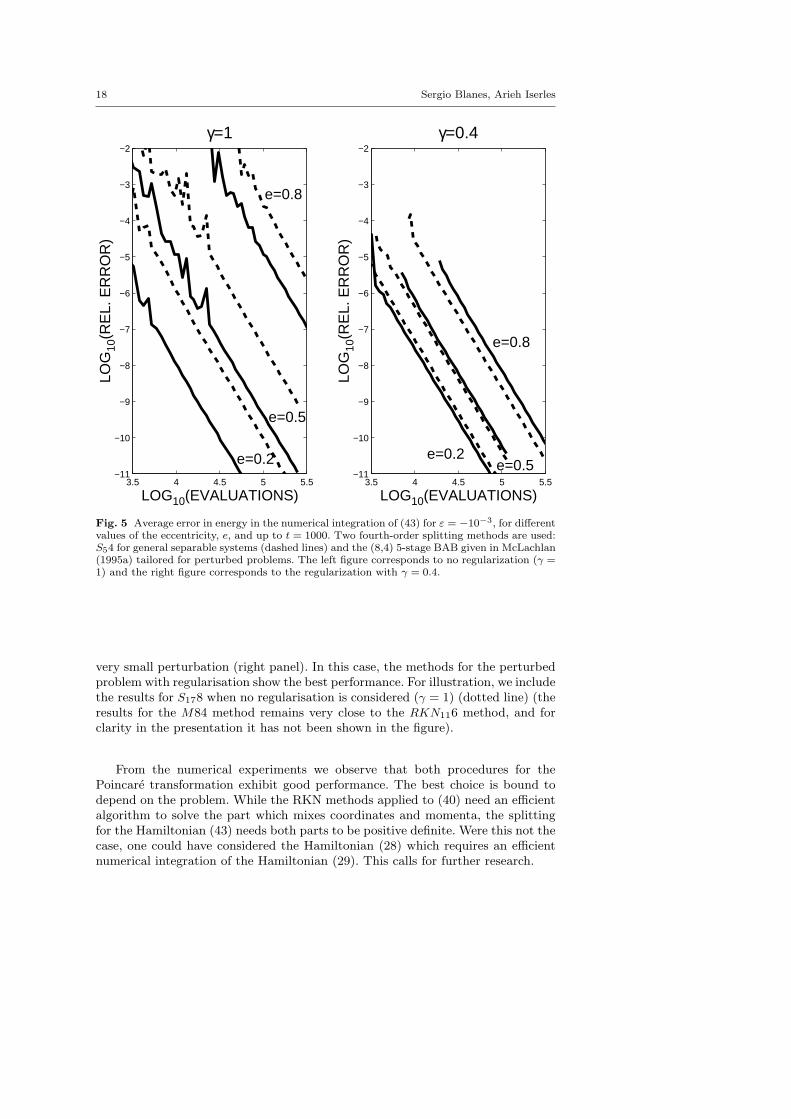
Fig. 5 Average error in energy in the numerical integration of (43) for ε = −10−3, for differentvalues of the eccentricity, e, and up to t = 1000. Two fourth-order splitting methods are used:S54 for general separable systems (dashed lines) and the (8,4) 5-stage BAB given in McLachlan(1995a) tailored for perturbed problems. The left figure corresponds to no regularization (γ =1) and the right figure corresponds to the regularization with γ = 0.4.
very small perturbation (right panel). In this case, the methods for the perturbedproblem with regularisation show the best performance. For illustration, we includethe results for S178 when no regularisation is considered (γ = 1) (dotted line) (theresults for the M84 method remains very close to the RKN116 method, and forclarity in the presentation it has not been shown in the figure).
From the numerical experiments we observe that both procedures for thePoincare transformation exhibit good performance. The best choice is bound todepend on the problem. While the RKN methods applied to (40) need an efficientalgorithm to solve the part which mixes coordinates and momenta, the splittingfor the Hamiltonian (43) needs both parts to be positive definite. Were this not thecase, one could have considered the Hamiltonian (28) which requires an efficientnumerical integration of the Hamiltonian (29). This calls for further research.

Explicit Adaptive Symplectic Integrators for solving Hamiltonian Systems 19
4 4.2 4.4 4.6 4.8 5−11
−10
−9
−8
−7
−6
−5e=0.8, ε=−10−3
LOG10(EVALUATIONS)
LOG
10(R
EL.
ER
RO
R)
3.5 4 4.5 5
−12
−11
−10
−9
−8
−7
−6
−5e=0.5, ε=−10−5
LOG10(EVALUATIONS)
LOG
10(R
EL.
ER
RO
R)
Fig. 6 Average error in energy in the numerical integration of (38) integrated using theS54, S96 and S178 methods applied to (43) with γ = 0.4 (dashed lines), and the RKN64and RKN116 methods applied to (40) with γ = 3/2 (solid lines). These methods can bedistinguished by the slope of the curves. Left panel: corresponds to the choice e = 0.8 andε = −10−3. Right panel: corresponds to the choice e = 0.5 and ε = −10−5. The results forS178 when no regularisation is considered (γ = 1) is also shown (dotted line).
4.3 The two-fixed-centres problem
We finally consider the two-dimensional two-fixed-centres problem
H =1
2(p2
1 + p22)− 2µ
r1− 2(1− µ)
r2, (45)
with r1 =√
(q1 − c)2 + q22 , r2 =
√(q1 + c)2 + q2
2 . We take µ = 0.4, c = 1 and
initial conditions q1 = 1/2, q2 = 0, p1 = 0, p2 =√
3 which has close approachesto one of the singularities (see Figure 7).

20 Sergio Blanes, Arieh Iserles
0.4 0.6 0.8 1 1.2 1.4 1.6 1.8 2 2.2−2
−1.5
−1
−0.5
0
0.5
1
1.5
2
q1
q 2
Fig. 7 Solution for the two-fixed-centres problem (45) for t ∈ [0, 1000] and parameters givenin the text .
For this problem we take the monitor function g = rγ1 rγ
2 for γ = 32 , and we take
the Sundman transformation with G(z) = 1/z and the splitting
d
dτ
q
p
t
z
=
1
zp
0
00
︸ ︷︷ ︸fA
+
0
0
0
−γ
(R1
r21
+R2
r22
)
︸ ︷︷ ︸fB
+
0
−g∇V (q)1
z0
︸ ︷︷ ︸fC
(46)
with R1 = (q1− c)p1 + q2p2, R2 = (q1 + c)p1 + q2p2. This corresponds, basically, tothe split (14), as proposed in Mikkola and Aarseth (2002), but separated in threeparts for simplicity.
We consider the S178 method as a composition of the symmetric second order(11) and we take a fictive time step such that the final real time, t = 1000, isreached with approximately 50000 evaluations of the potential, and measure theerror in energy along the time integration.
We repeated the numerical experiment replacing the term −g∇V (q) in fC ,which is not the gradient of a potential, by −(∇V (q))/z, which preserves sym-plecticity. The results are shown in Fig. 8 where the highest performance of thesymplectic scheme is clear. As previously mentioned, this deserves further investi-gation.
If one considers the Poincare transformation then RKN symplectic methods canbe used if the Hamiltonian K1 = rγ
1 rγ2 (p2
1 + p22)/2 is exactly solved, or numerically
solved up to high accuracy. For this problem it is clear that we can not use a

Explicit Adaptive Symplectic Integrators for solving Hamiltonian Systems 21
1 2 3−6.5
−6
−5.5
−5
−4.5
−4
−3.5
−3
−2.5
−2
−1.5g grad(V)
LOG10(t)
LOG
10(E
RR
OR
EN
ER
GY
)
1 2 3−6.5
−6
−5.5
−5
−4.5
−4
−3.5
−3
−2.5
−2
−1.5(1/z) grad(V)
LOG10(t)
LOG
10(E
RR
OR
EN
ER
GY
)
Fig. 8 Error in energy along the time integration for the two-fixed-centres problem (45) forthe split (46) (left panel) and when the term −gV (q) in fC is replaced by −(∇V (q))/z (rightpanel) .
canonical transformation to solve it, but the logarithmic method can be used veryeasily to high accuracy and low computational cost.
5 Conclusions
We have considered the Sundman and the Poincare transformation for the numer-ical integration of separable Hamiltonian systems evolving at different time scales.We have considered both transformation in their general form. This allowed usto obtain, in a simple form, most algorithms proposed in the recent literature asparticular cases. We have also constructed new highly efficient methods, displayingtheir best performance when a high accuracy is desired.
The numerical experiments suggest that, in general, both the Sundman and thePoincare transformations provide similar accuracy if an appropriate regularizationfunction is chosen (which can differ in each case) and the same splitting methodis used in both cases. The main difference remains in the fact that the Poincaretransformation allows, in some cases, to retain the structure of the original Hamil-tonian (e.g. quadratic in momenta or near-integrable) and one can use splittingmethods tailored for these problems. This requires the numerical integration of

22 Sergio Blanes, Arieh Iserles
new Hamiltonian functions with a relatively simple and very particular structurewhose efficient integration allows to end up with highly efficient algorithms. TheSundman transformation is, however, more general and can be easily used on nonHamiltonian systems.
The results presented in this work easily extend to time-dependent potentialfunctions V (q, t) by considering the time as a new coordinate as well as to otherseparable Hamiltonian functions.
References
Blanes S, Budd CJ (2004) High order symplectic integrators for perturbed hamil-tonian systems. Celestial Mechanics and Dynamical Astronomy 89:383–405
Blanes S, Budd CJ (2005) Adaptive geometric integrators for hamiltonian prob-lems with approximate scale invariance. SIAM J Sci Comput 26:1089–1113
Blanes S, Moan PC (2002) Practical symplectic partitioned runge–kutta andrunge–kutta–nystrom methods. J Comp Appl Math 142:313–330
Blanes S, Casas F, Ros J (1999) Extrapolation of symplectic integrators. CelestialMechanics and Dynamical Astronomy 75:149–161
Blanes S, Casas F, Murua A (2008) Splitting and composition methods in thenumerical integration of differential equations. Bol Soc Esp Mat Apl 45:89–145
Bond SD, Leimkuhler B (1998) Time-transformations for reversible variable step-size integration. Numerical Algorithms 19:55–71
Budd CJ, Leimkuhler B, Piggott MD (2001) Scaling invariance and adaptivity.Appl Numer Math 39:261–288
Calvo MP, Sanz-Serna JM (1993) The development of variable-step symplecticintegrators, with applications to the two-body problem. SIAM J Sci Comput14:936–952
Calvo MP, Sanz-Serna JM, Lopez-Marcos MA (1998) Variable step implementa-tions of geometric integrators. Appl Numer Math 28:1–16
Chan RPK, Murua A (2000) Extrapolation of symplectic methods for hamiltonianproblems. Appl Numer Math 34:189–205
Creutz M, Gocksch A (1989) Higher-order hybrid monte carlo algorithms. PhysRev Lett 63:9–12
Gladman B, Duncan M, Candy J (1991) Symplectic integrators for long-termintegrations in celestial mechanics. Celestial Mechanics 52:221–240
Hairer E (1997) Variable time step integration with symplectic methods. ApplNumer Math 25:219–227
Hairer E, Soderlind G (2005) Explicit, time reversible, adaptive stepsize control.SIAM J Sci Comput 26:1838–1851
Hairer E, Lubich C, Wanner G (2006) Geometric Numerical Integration. Structure-Preserving Algorithms for Ordinary Differential Equations, vol 31, Second edn.Springer-Verlag
Holder T, Leimkuhler B, Reich S (2001) Explicit variable step-size and time-reversible integration. Appl Numer Math 39:367–377
Huang W, Leimkuhler B (1997) The adaptive verlet method. SIAM J Sci Comput18:239–256
Iserles A (2008) A First Course in the Numerical Analysis of Differential Equations,Second edn. Cambridge University Press

Explicit Adaptive Symplectic Integrators for solving Hamiltonian Systems 23
Kinoshita H, Yoshida H, Nakai H (1991) Symplectic integrators and their appli-cation to dynamical astronomy. Celestial Mechanics and Dynamical Astronomy50:59–71
Laskar J, Robutel P (2001) High order symplectic integrators for perturbed hamil-tonian systems. Celestial Mechanics and Dynamical Astronomy 80:39–62
Leimkuhler B, Reich S (2004) Simulating Hamiltonian Dynamics. Cambridge Uni-versity Press
McLachlan RI (1995a) Composition methods in the presence of small parameters.BIT Numerical Mathematics 35:258–268
McLachlan RI (1995b) On the numerical integration of ordinary differential equa-tions by symmetric composition methods. SIAM J Sci Comput 16(1):151–168
McLachlan RI, Quispel RGW (2002) Splitting methods. Acta Numerica 11:341–434
McLachlan RI, Quispel RGW (2006) Geometric integrators for odes. J Phys A:Math Gen 39:5251–5285
Mikkola S (1997) Practical symplectic methods with time transformation for thefew-body problem. Celestial Mechanics and Dynamical Astronomy 67:145–165
Mikkola S, Aarseth S (2002) A time-transformed leapfrog scheme. Celestial Me-chanics and Dynamical Astronomy 84:343–354
Mikkola S, Tanikawa K (1999) Explicit symplectic algorithms for time-transformedhamiltonians. Celestial Mechanics and Dynamical Astronomy 74:287–295
Preto M, Tremaine S (1999) A class of symplectic integrators with adaptive timestep for separable hamiltonian systems. Celestial Mechanics and Dynamical As-tronomy 118:2532–2541
Sanz-Serna JM, Calvo MP (1994) Numerical Hamiltonian Problems. Chapmanand Hall
Skeel R (1993) Variable step size destabilizes the stormer/leapfrog/verlet method.BIT Numerical Mathematics 33:172–175
Sophroniou M, Spaletta G (2005) Derivation of symmetric composition constantsfor symmetric integrators. Optimization Methods Software 20:597–613
Stiefel EL, Scheifel G (1971) Linear and regular celestial mechanics. Springer,Berlin
Suzuki M (1990) Fractal decomposition of exponential operators with applica-tions to many-body theories and monte carlo simulations. Physics Letters A146(6):319 – 323
Wisdom J, Holman M (1991) Symplectic maps for the n-body problem. Astro-nomical Journal 102:1528–1538
Yoshida H (1990) Construction of higher order symplectic integrators. PhysicsLetters A 150(5-7):262 – 268