Explain how managers should determine the optimal method ... · of production by applying an...

OBJECTIVE

•Explain how managers should determine the optimal method of production by applying an understanding of production processes

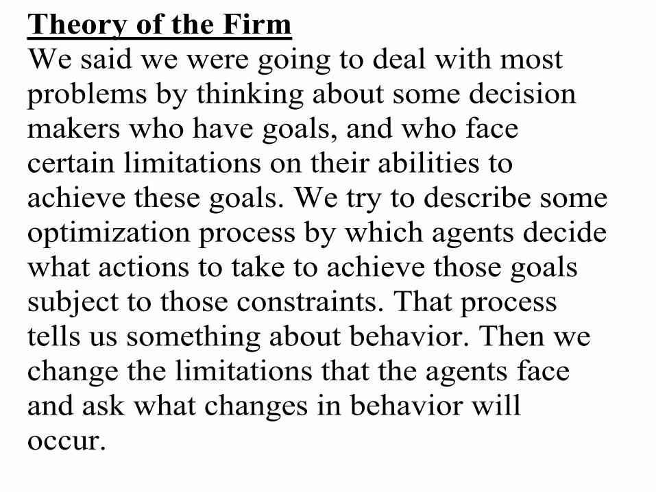
Theory of the Firm

We said we were going to deal with most

problems by thinking about some decision

makers who have goals, and who face

certain limitations on their abilities to

achieve these goals. We try to describe some

optimization process by which agents decide

what actions to take to achieve those goals

subject to those constraints. That process

tells us something about behavior. Then we

change the limitations that the agents face

and ask what changes in behavior will

occur.

In the case of consumers, they have preferences and utility

functions and they face a budget constraint. We asked what

were the changes in behavior due to changes in the budget

constraint.

This same methodology can be used to discuss the theory of

the firm. There are different environments in which a

firm operates. We will talk about some of those different

paradigms (competitive firms, monopolistic firms,

oligopolistic firms). Within some of those environments we

will talk about how a change in the limitations could lead

to a change in behavior. We can ask for example, if a

change in the prices the firm pays for its inputs or charges

for its outputs may lead to a change in what the firm

chooses to do.

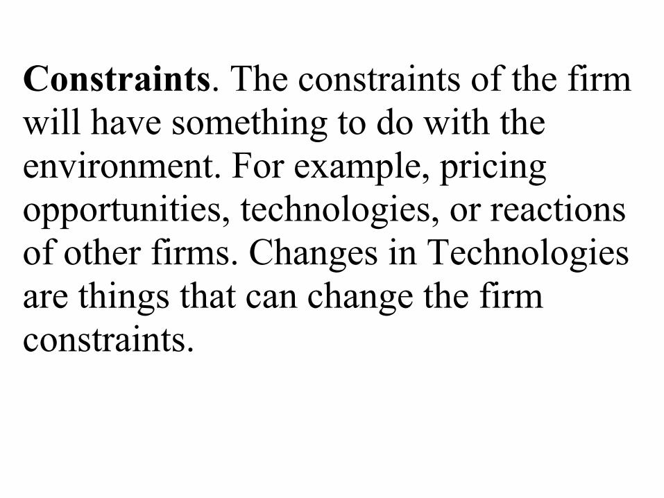
Constraints. The constraints of the firm

will have something to do with the

environment. For example, pricing

opportunities, technologies, or reactions

of other firms. Changes in Technologies

are things that can change the firm

constraints.

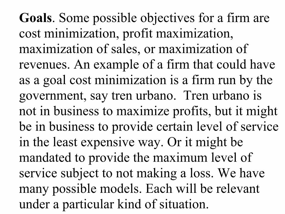
Goals. Some possible objectives for a firm are

cost minimization, profit maximization,

maximization of sales, or maximization of

revenues. An example of a firm that could have

as a goal cost minimization is a firm run by the

government, say tren urbano. Tren urbano is

not in business to maximize profits, but it might

be in business to provide certain level of service

in the least expensive way. Or it might be

mandated to provide the maximum level of

service subject to not making a loss. We have

many possible models. Each will be relevant

under a particular kind of situation.

Behavior. We will be asking questions such

as how much does the firm produce, what

price does it charge, and how many inputs

does it buy.

Technology

Production functions.

A production function is a function that states

the relationship between a set of inputs the firm

uses and outputs.

When we think of the case of the consumer, the

production function are similar to utility

functions. Utility functions allow us to derive

utility as function of goods consumed while

production functions allow us to derive a level

of production from a given level of inputs.

Output=f(inputs)=Q=f(x1,x2,………,xn)

PRODUCTION PROCESSES

• Production processes include all activities associated with providing goods and services, including

• Employment practices

• Acquisition of capital resources

• Product distribution

• Managing intellectual resources

PRODUCTION PROCESSES

• Production processes define the relationships between resources used and goods and services produced per time period.

• Managers exert control over production costs by understanding and managing production technology.

PRODUCTION FUNCTION WITH ONE VARIABLE INPUT

• A production function shows the maximum amount that can be produced per time period with the best available technology from any given combination of inputs.

• Table

• Graph

• Equation


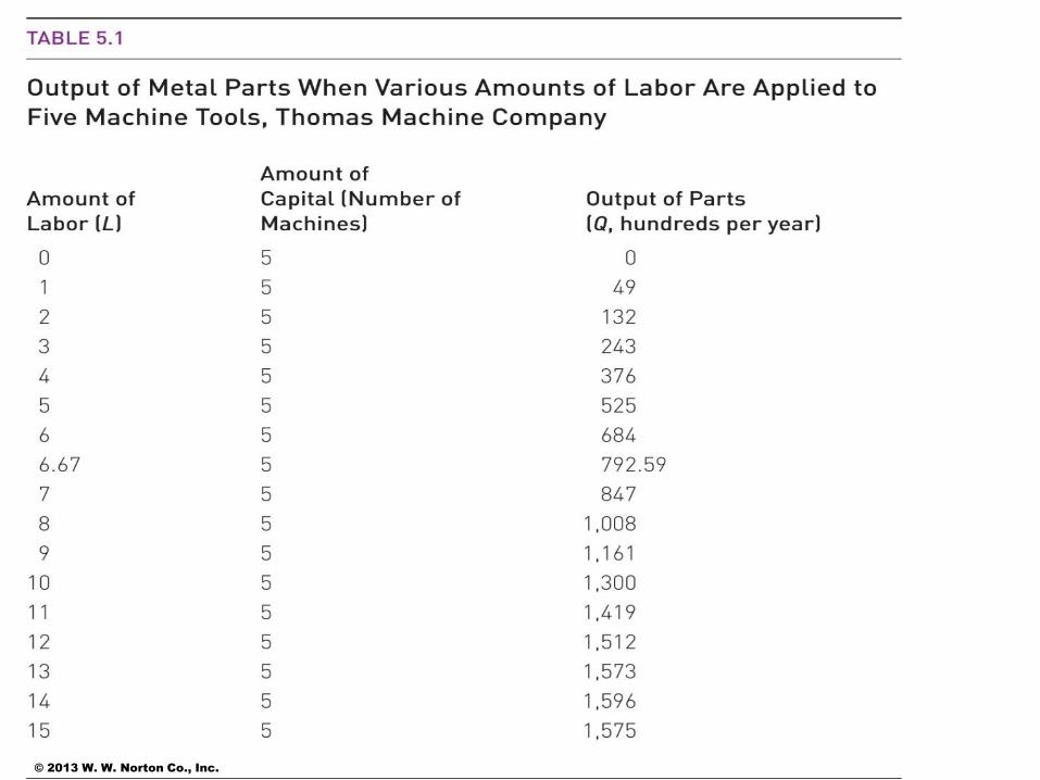
• Production Function Example

oQ = f(X1, X2) • Q = Output rate

• X1 = Input 1 usage rate


oQ = 30L + 20L2 – L3 • Q = Hundreds of parts produced per year

• L = Number of machinists hired

• Fixed Capital = Five machine tools

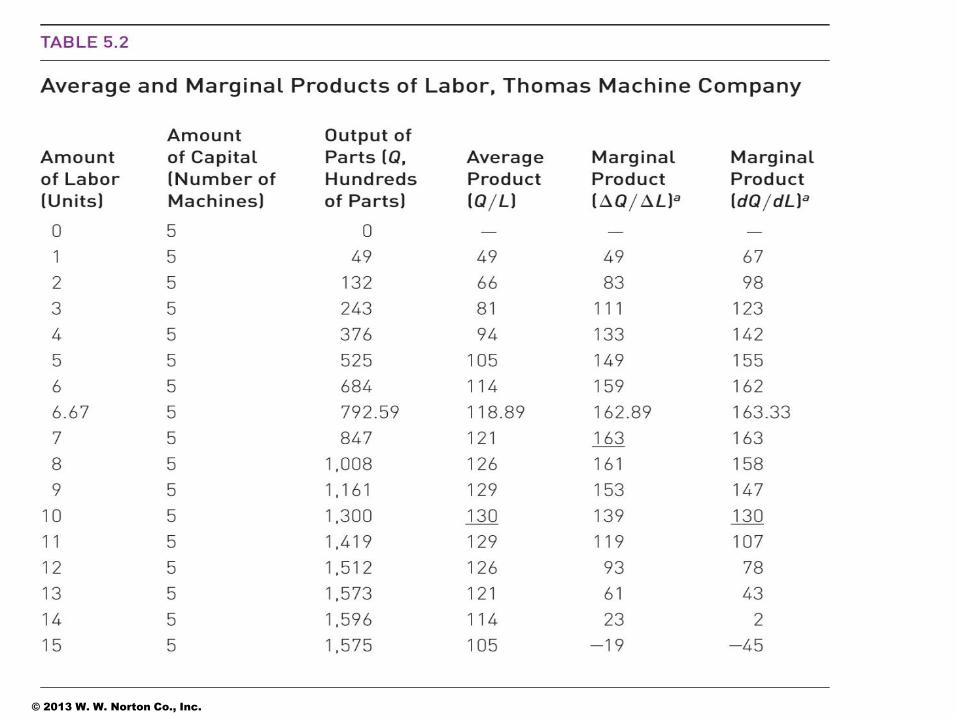
RELATIONSHIP BETWEEN TOTAL OUTPUT AND AMOUNT OF LABOR USED ON FIVE MACHINE TOOLS, THOMAS MACHINE COMPANY

Managerial Economics, 8e

Copyright @ W.W. & Company 2013


• Unit Functions

• Average Product of Labor = APL = Q/L • Common measuring device for estimating the units of output, on average, per

worker


• Unit Functions (cont’d)

• Marginal Product of Labor = MPL = Q/L • Metric for estimating the efficiency of each input in which the input’s MP is equal

to the incremental change in output created by a small increase in the input

• Using calculus (assumes that labor can be varied continuously): MP = dQ/dL


• Unit Functions (cont’d) • Unit function examples from Q = 30L + 20L2 – L3

• APL = 30 + 20L – L2

• Using calculus: MPL = 30 + 40L – 3L2

• APL is at a maximum, and MPL = APL, at L = 10 and MPL = APL = 130

• MPL is at a maximum at L = 6.67 and MPL = 163.33


• Unit Functions (cont’d)

•Why does MPL = APL when APL is at a maximum? •If MPL > APL, then APL must be increasing •If MPL < APL, then APL must be decreasing

AVERAGE AND MARGINAL PRODUCT CURVES FOR LABOR



THE PRODUCTIONN FUNCTION WITH TWO VARIABLE INPUTS

• Q = f(X1, X2)

• Q = Output rate



• AP1 = Q/X1 and MP1 = Q/X1 or dQ/dX1

• AP2 = Q/X2 and MP2 = Q/X2 or dQ/dX2

Below we have an example of a two

variable Cobb-Douglas production function.

q = f(K,L)=KL

Where K is capital and L is labor. Like

utility we can learn a lot by analyzing these

functions on the margin.

Marginal prodauct

Marginal product is the added production

gained from increasing one input. The

concept is similar to Marginal Utility.

lL

KK

fl

qMP

fk

qMP

THE LAW OF DIMINISHING MARGINAL RETURNS

• Law of diminishing returns

•When managers add equal increments of an input while holding other input levels constant, the incremental gains to output eventually get smaller.

Diminishing Marginal Product

For the most part we will assume diminishing

marginal product in much the same way we assumed

diminishing marginal utility. What this means is as

we add more inputs production may go up but the

last unit of input adds less to production than the

unit of input before. What this means is that the first

derivative may be positive but the second should be

negative.

0

0

2

2

2

2

LL

L

kk

K

fL

q

L

MP

fk

q

K

MP

As we have seen Average product

AP is

L

Lkf

L

qAPL

),(

K

LKf

K

qAPK

),(

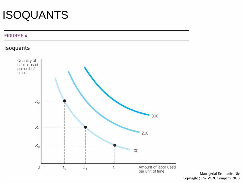
ISOQUANTS

• Isoquant: Curve showing all possible (efficient) input bundles capable of producing a given output level

• Graphically constructed by cutting horizontally through the production surface at a given output level

ISOQUANTS



ISOQUANTS

• Properties

• Isoquants farther from the origin represent higher output levels.

• Given a continuous production function, every possible input bundle is on an isoquant and there is an infinite number of possible input combinations.

• Isoquants slope downward to the left and are convex to the origin.

Isoquants

Say we have a single output good and two

inputs y1 and y2. We may want to look at

combinations of those two inputs that can

produce the same level of output. Say the

points in figure A below are two ways we

can produce the same amount of omelets.

Each one uses different proportions of eggs

and labor. One uses a relatively smaller

amount of eggs and more labor than the other

one.

y

y1

2

Figure A

I may want to assume constant returns to

scale. This would mean that I can produce

anywhere along the rays from the origin in

figure below. So far, all my technology has

described is a production set that consists of

these 2 rays. (The arrows in Figure B are

just referring to the fact that both points

produce 1 omelet.)

y

y1

21 omelete

We may also want to assume convexity.

This would mean that I can also produce one

omelet using a linear combination of these

two techniques. For example, I can produce

half omelet using one technique and another

half omelet using the other technique. If we

have additivity, we can produce a whole

omelet by producing half an omelet in each

particular way (see figure C). Or I can

produce a whole omelet using a convex

combination of these two techniques.

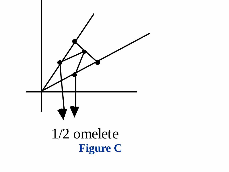
1/2 omeleteFigure C

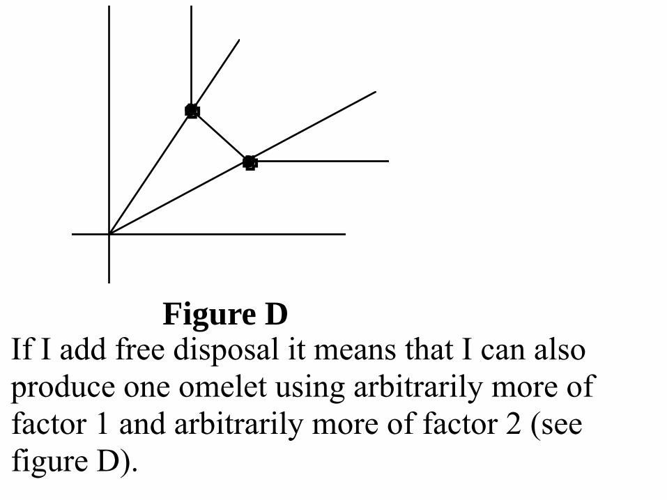
If I add free disposal it means that I can also

produce one omelet using arbitrarily more of

factor 1 and arbitrarily more of factor 2 (see

figure D).

Figure D

If I had three different ways of producing

omelets by taking convex combinations we

would get figure E.

Figure E

I am going to produce a convex hull from all

the different activities that are available to me.

If I have several ways of producing one

omelet, the lower hull would be all the

efficient ways of producing a single omelet

(see figure F). In general, if I have lots of

different activities, ultimately I would end up

with some convex surface like the one in

figure F, and it would be called the unit

isoquant.

Figure F

In general an isoquant depics a situation

where the same level of production can be

achieved using different combinations of

inputs.

q=150

q=100

Notice this isoquant looks a lot like an

indifference curve. The difference is here we

are analyzing production while we used the

indifference curve to analyze utility. Of course

the indifference curve is derived from the

utility function while the isoquant is derived

from the production function.

MARGINAL RATE OF TECHNICAL SUBSTITUTION

•Marginal rate of technical substitution (MRTS): Shows the rate at which one input is substituted for another (with output remaining constant)

•Q = f(X1, X2)

• MRTS = –X2/X1 with Q held constant and X2 on the vertical axis

• MRTS = MP1/MP2

• MRTS = Absolute value of the slope of an isoquant


• MRTS and isoquants (with X2 on the vertical axis)

• If the MRTS is large, it takes a lot of X2 to substitute for one unit of X1, and isoquants will be steep.

• If the MRTS is small, it takes little X2 to substitute for one unit of X1, and isoquants will be flat.


• MRTS and isoquants (with X2 on the vertical axis) (cont’d)

•If X1 and X2 are perfect substitutes, MRTS is constant, and isoquants will be straight lines.

•If X1 and X2 are perfect complements, no substitution is possible, MRTS is undefined, and isoquants will be right angles.

ISOQUANTS IN THE CASE OF FIXED PROPORTIONS




• Ridge Lines

•Ridge lines: the lines that profit-maximizing firms operate within because outside them, marginal products of inputs are negative

•Economic region of production is located within the ridge lines.

ECONOMIC REGION OF PRODUCTION



Marginal Rate of Technical Substitution

(MRTS)

The MRTS is simply the rate at which the

firm has to substitute one input for another

while keeping production constant. In other

words it is the slope of the isoquant. Again

it is a very similar concept to the marginal

rate of substitution in utility theory.

MRTS dK

dL qq0

To derive it take the total differential of the

production function. Notice we end up with

the marginal product of labor and capital

multiplied by the change in labor and capital

respectively.

dq f

LdL

f

KdK MPLdL MPKdK

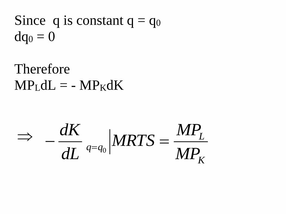
Since q is constant q = q0

dq0 = 0

Therefore

MPLdL = - MPKdK

K

Lqq

MP

MPMRTS

dL

dK 0

RETURNS TO SCALE

This concept allows us to exam what happens

to production when all inputs are increase by

the same percentage.

f (tK, tL) = tf(K, L) Constant

f (tK, tL) < tf(K, L) Decreasing

f (tK, tL) > tf(K, L) Increasing

Explain how managers should determine the optimal method ... · of production by applying an...

Documents

Transcript of Explain how managers should determine the optimal method ... · of production by applying an...