Expert Meeting: Recommended Approaches to · PDF fileExpert Meeting: Recommended Approaches to...

Expert Meeting: Recommended Approaches to Humidity Control in High Performance Homes Armin Rudd Building Science Corporation (BSC)

July 2013

NOTICE

This report was prepared as an account of work sponsored by an agency of the United States government. Neither the United States government nor any agency thereof, nor any of their employees, subcontractors, or affiliated partners makes any warranty, express or implied, or assumes any legal liability or responsibility for the accuracy, completeness, or usefulness of any information, apparatus, product, or process disclosed, or represents that its use would not infringe privately owned rights. Reference herein to any specific commercial product, process, or service by trade name, trademark, manufacturer, or otherwise does not necessarily constitute or imply its endorsement, recommendation, or favoring by the United States government or any agency thereof. The views and opinions of authors expressed herein do not necessarily state or reflect those of the United States government or any agency thereof.

Available electronically at http://www.osti.gov/bridge

Available for a processing fee to U.S. Department of Energy and its contractors, in paper, from:

U.S. Department of Energy Office of Scientific and Technical Information

P.O. Box 62 Oak Ridge, TN 37831-0062

phone: 865.576.8401 fax: 865.576.5728

email: mailto:[email protected]

Available for sale to the public, in paper, from: U.S. Department of Commerce

National Technical Information Service 5285 Port Royal Road Springfield, VA 22161 phone: 800.553.6847

fax: 703.605.6900 email: [email protected]

online ordering: http://www.ntis.gov/ordering.htm

Printed on paper containing at least 50% wastepaper, including 20% postconsumer waste

http://www.osti.gov/bridge

mailto:[email protected]

mailto:[email protected]

http://www.ntis.gov/ordering.htm

iii

Expert Meeting: Recommended Approaches to Humidity Control in High Performance Homes

Prepared for:

The National Renewable Energy Laboratory

On behalf of the U.S. Department of Energy’s Building America Program

Office of Energy Efficiency and Renewable Energy

15013 Denver West Parkway

Golden, CO 80401

NREL Contract No. DE-AC36-08GO28308

Prepared by:

Armin Rudd

Building Science Corporation

30 Forest Street

Somerville, MA 02143

NREL Technical Monitor: Cheryn Engebrecht

Prepared under Subcontract No. KNDJ-0-40337-00

July 2013

iv

Acknowledgements

The author appreciates the presentations made by the invited speakers including: Hugh Henderson of CDH Energy Corp.; Philip Fairey of Florida Solar Energy Center; and Michael Sypolt of IBACOS.

Definitions

BSC Building Science Corporation

AHRI Air Conditioning Heating and Refrigeration Institute

AHAM Association of Home Appliance Manufacturers

RH Relative humidity

NRC Natural Resources Canada

USDOE United States Department of Energy

NREL National Renewable Energy Laboratory

CFI Central-fan-integrated [supply ventilation]

ERV Energy recovery ventilator

HRV Heat recovery ventilator

v

[This page left blank]

vi

Table of Contents Acknowledgements ................................................................................................................................... iv Definitions ................................................................................................................................................... iv List of Figures ........................................................................................................................................... vii List of Tables ............................................................................................................................................ viii 1 Introduction ........................................................................................................................................... 1 2 Logistics ................................................................................................................................................ 2 3 Research Questions ............................................................................................................................. 2 4 Objectives .............................................................................................................................................. 3 5 Agenda ................................................................................................................................................... 4 6 Agenda Summaries .............................................................................................................................. 4

ASHRAE RP 1449: Energy Efficiency and Cost Assessment of Humidity Control Options for Residential Buildings .....................................................................................................4

Humidity Control and Ventilation ...........................................................................................17 EnergyPlus Humidity Control and Ventilation Modeling Analysis ........................................25

7 Answers to Research Questions ...................................................................................................... 29 8 Action Items ........................................................................................................................................ 32 9 References .......................................................................................................................................... 34

vii

List of Figures Figure 1. Computer modeling improvements allowing more realistic simulation results. ................. 5 Figure 2. Simulation framework that allows for multiple temperature control, humidity control,

ventilation, and fan recirculation systems to operate at the same time. ........................................ 5 Figure 3. Simulation framework that allows for multiple temperature control, humidity control,

ventilation, and fan recirculation systems to operate at the same time. ........................................ 6 Figure 4. Calculation of the combined airflow of infiltration, duct leakage, and balanced and

unbalanced ventilation. ........................................................................................................................ 7 Figure 5. Conventional cooling system and indoor temperature and RH response with heating,

floating, and cooling hours in the same day. .................................................................................... 7 Figure 6. RH limit expressed as hours over 60% RH and 4 hour events over 60% RH. ...................... 8 Figure 7. Impact of exhaust ventilation rate at 50%, 100% and 150% of the ASHRAE Standard 62.2-

2010 whole-building ventilation rate. ................................................................................................. 9 Figure 8. Simulation results for enhanced Systems modeled in HERS 70 level houses. ................. 10 Figure 9. A check of the simulation response with moisture capacitance turned off (set to zero). . 11 Figure 10. Measured and simulated indoor vs. outdoor humidity trends with indoor moisture

capacitance. ........................................................................................................................................ 12 Figure 11. The impact of overcooling by three degrees “sweeps” the higher RH hours down and to

the left. ................................................................................................................................................. 12 Figure 12. Locating the air distribution system ducts inside conditioned space saves overall

energy, but also increases the need for supplemental dehumidification. ................................... 13 Figure 13. In Miami, hours of elevated indoor humidity occur mostly in morning hours between

late November and March. ................................................................................................................. 14 Figure 14. Hours of elevated indoor humidity is strongly related to internal moisture gains and

internal sensible gains. ...................................................................................................................... 15 Figure 15. Hours of elevated indoor humidity is weakly related to moisture capacitance. .............. 15 Figure 16. Hours of elevated indoor humidity is strongly related to heating setpoint. ..................... 16 Figure 17. Interactive Internet access is made available to retrieve customized sets of the

simulation data. .................................................................................................................................. 16 Figure 18. Twelve cities and five climate zones simulated for a ventilation study including

humidity impacts. ............................................................................................................................... 17 Figure 19. Outline of simulation prototype assumptions. .................................................................... 18 Figure 20. Internal sensible (16.9 kWh/day) and latent gains schedule used in the simulations. .... 19 Figure 21. For a week at the end of June and beginning of July on Orlando, the cooling system

and space RH is showing an expected response. .......................................................................... 20 Figure 22. Hours above 60% RH for exhaust and ERV ventilation in Orlando. .................................. 20 Figure 23. Hours above 60% by climate and space conditioning mode. ............................................ 21 Figure 24. Hours of elevated indoor RH is a strong function of the selected RH limit and climate. 22 Figure 25. ASHRAE 62.2-2010 addendum r ventilation rate raises median RH compared to

conventional dwelling without mechanical ventilation. ................................................................. 22 Figure 26. Predicted required moisture removal by supplemental dehumidification, by ventilation

system type (energy recovery ventilator, exhaust, CFI supply). ................................................... 23 Figure 27. Predicted cost of supplemental dehumidification. .............................................................. 24 Figure 28. NREL BEopt E+ program used to generate the building geometry and the base IDF files

(input description). ............................................................................................................................. 25 Figure 29. Indoor RH vs. hour of year comparison between EnergyPlusPlus (blue symbols) and

EnergyGauge USA (V3.0.01P) simulation results. .......................................................................... 26 Figure 30. Energy consumption results by ventilation system type, ventilation rate, and building

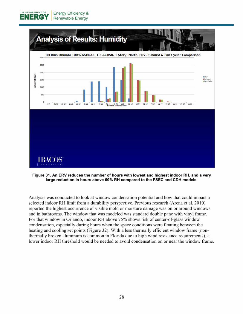
enclosure tightness. ........................................................................................................................... 27 Figure 31. An ERV reduces the number of hours with lowest and highest indoor RH, and a very

large reduction in hours above 60% RH compared to the FSEC and CDH models. .................... 28 Figure 32. Window condensation potential during Orlando floating hours ....................................... 29 Figure 33. Overview of recommended dehumidifier test conditions. ................................................. 33

Unless otherwise noted, all figures were created by BSC.

viii

List of Tables Table 1. List of meeting participants ......................................................................................................... 2 Table 2. Expert Meeting Agenda ................................................................................................................ 4 Unless otherwise noted, all tables were created by BSC.

1

1 Introduction

As homes get more energy efficient, cooling systems have longer off-times due to lowered sensible heat gain. Overall, this is good, and produces a significant net energy and cost savings. However, this situation requires a change to conventional residential space conditioning system design in humid climates. While the sensible cooling load is lower, and can be dealt with in the conventional way, the latent (moisture) load in high performance homes remains nearly unchanged due to ventilation requirements and internal moisture generation by occupants and their activities. Therefore, at times when there is no need to lower the space air temperature, supplemental dehumidification will be required to maintain the relative humidity (RH) below acceptable levels.

Extensive field testing was done with builder partners in Texas and Florida in 2001 to 2007 (Rudd et al. 2003, BSC 2004, Rudd et al. 2005). That testing revealed that supplemental dehumidification was required in high performance Building America-level homes in order to maintain indoor RH below 60% year-round.

Off-the-shelf, stand-alone supplemental dehumidification systems were employed to address this problem while working with manufacturing partners on supplemental dehumidification integrated with the central space conditioning system. These companies began to offer integrated supplemental dehumidification solutions that allow year-round indoor RH control between 50% and 60%. This was intended to enable further reduction in sensible cooling load. through further efficiency improvements, without the risk of elevated indoor humidity.

While these advancements have been important and needed in the residential space conditioning industry, supplemental dehumidification technology continues to improve and evolve, and the market for these products is still in its infancy. Design capacity prediction is subject to many unknowns and requires continued research to fully quantify.

Models that can accurately simulate the performance of humidity control systems in high performance buildings are needed to understand a wide range of scenarios related to the economics and operational success of low-energy homes with supplemental dehumidification. Simulation of supplemental dehumidification needs and performance in buildings is complex. It requires a model that controls both indoor temperature and RH, and depends on many still somewhat sketchy inputs, such as: internal moisture generation and other moisture loads including effects of construction moisture drying and rain wetting under solar loading; building moisture capacitance and the effects of building material moisture adsorption/desorption under solar loading; and detailed dehumidification equipment performance maps. This capability is improving but still has a long way to go to be adequately integrated into commonly used building design and performance rating programs.

Building Science Corporation (BSC) hosted an expert meeting, “Recommended Approaches to Humidity Control in High Performance Homes,” on October 16, 2012, in Westford, Massachusetts, to bring together experts in the field of residential humidity control to address modeling issues for dehumidification.

2

2 Logistics

The expert meeting was held at the Westford Regency Inn and Conference Center, in Westford, Massachusetts, on October 16, 2012. The meeting was also made available to attendees by webinar, and was recorded. See Table 1 for a list of attendees.

Table 1. List of Meeting Participants.

3 Research Questions

A list of research questions that were compiled and distributed with the meeting invitation is as follows:

• What are the important humidity control conclusions from recent residential dehumidification systems modeling, with a wide range of building and equipment sensitivity, using a customized <2 minute time-step TRNSYS model with temperature and humidity control?

• What are the important humidity control conclusions from recent residential ventilation modeling efforts using the temperature and humidity control logic of the Energy Plus version of the NREL BEopt program?

• What are the important indoor humidity conclusions that can be drawn from recent residential ventilation modeling efforts using the temperature-only control logic of the FSEC EnergyGauge USA program?

Last name First name Company EmailAttended In Person (P)

or by Webinar (W)

Bergey Daniel BSC [email protected] PBloemer John Research Products [email protected] PFairey Philip FSEC [email protected] PHarriman Lew Mason Grant [email protected] PHenderson Hugh CDH Energy [email protected] PKerrigan Philip BSC [email protected] PMetzger Cheryn NREL [email protected] PPettit Betsy BSC [email protected] PPrahl Duncan IBACOS [email protected] PRudd Armin BSC [email protected] PSypolt Michael IBACOS [email protected] PWinkler John NREL [email protected] PCottrell Glenn IBACOS [email protected] WDentz Jordan The Levy Partnership [email protected] WGriffiths Dianne Steven Winter Associates [email protected] WGrisolia Anthony IBACOS [email protected] WHudon Kate NREL [email protected] WMittereder Nick Ibacos [email protected] WPuttagunta Srikanth Steven Winter Associates [email protected] WTabares Paulo NREL [email protected] W

3

• How do the results from these different programs compare?

• Is it generally agreed that controlling to less than 60% RH is the appropriate humidity control point for high performance homes, and why?

• Is it generally agreed that annual hours above 60% RH is the appropriate humidity control performance metric to use to compare system performance and to compare required supplemental dehumidification energy? Does that metric give generally the same result as looking at 4-hour and 8-hour events above 60% RH?

• For a range of climates, ventilation systems, and space conditioning equipment in high performance homes, what is the magnitude of hours above 60% RH, the magnitude of supplemental dehumidification energy required to control to less than 60% RH, the time of year occurrence of elevated indoor humidity and supplemental dehumidification, and the space conditioning mode (heating, cooling, floating) during which most periods of elevated indoor humidity and supplemental dehumidification occur?

4 Objectives

The topic of this meeting was “Recommended Approaches to Humidity Control in High Performance Homes,” and focused on dehumidification requirements. Presentations and discussions centered on computer simulation and field experience with these systems, with the goal of developing foundational information to support the development of a Building America Measure Guideline on this topic.

The expert meeting was designed to bring together experts in the field of residential indoor humidity control by dehumidification to discuss the following objectives:

• Compare and contrast the state-of-the art in modeling residential supplemental dehumidification requirements in high performance homes.

• Come to agreement on an acceptable RH control system within a model and the primary metric to be used for evaluating the success of a given humidity control system.

• Quantitatively identify general trends as to the performance of, and cost to operate, supplemental dehumidification systems in high performance homes in humid climates.

4

5 Agenda

Table 2 shows the expert meeting agenda.

Table 2. Expert Meeting Agenda.

Time Speaker Topic 8:00 to 8:10 Armin Rudd

Building Science Corp Welcome and Introduction

8:10 to 9:00 Hugh Henderson CDH Energy Corp

ASHRAE RP 1449 Energy Efficiency and Cost Assessment of Humidity Control Options for Residential Buildings

9:00 to 9:50 Philip Fairey Florida Solar Energy Center

Humidity Control and Ventilation

9:50 to 10:00 Break

10:00 to 10:50 Michael Sypolt and Duncan Prahl IBACOS

EnergyPlus Humidity Control and Ventilation Modeling Analysis

10:50 to 12:00 Armin Rudd Building Science Corp

Facilitated Open Discussion, Action Items, and Final Remarks

6 Agenda Summaries

Discussions occurred during and after each of the three invited presentations and in the facilitated discussion period that followed.

ASHRAE RP 1449: Energy Efficiency and Cost Assessment of Humidity Control Options for Residential Buildings (Hugh Henderson, CDH Energy Corp.)

A number of fundamental computer modeling improvements were made to the TRNSYS/TRNSED model that CDH had previously developed for desiccant and dehumidifier systems. The model improvements, listed in Figure 1, allowed for more accurate, real-world simulation results. The short time-step model allowed precise determination of when mechanical equipment would be on or off according to actual control strategies. Referring to Figure 2, space conditioning equipment, ventilation equipment, and dehumidification equipment could all be operating at the same time, with all the heat and moisture consequences accounted for in the same simulation time interval.

5

Modeling Approach• Using TRNSYS model first developed for

Desiccant and DH systems • Uses small time step (72 sec)

– No more part load curves (either ON or OFF)– Thermostat dynamics (for cooling)– Detailed control of all components (e.g., CFIS)

• Type 56 for multi-zone building– Combined duct leakage & infiltration calcs

• Robust equipment models (performance maps)

Figure 1. Computer modeling improvements allowing more realistic simulation results.

Updated Simulation Framework

Figure 2. Simulation framework that allows for multiple temperature control, humidity control, ventilation, and fan recirculation systems to operate at the same time.

6

Moisture evaporation from wet cooling coils is modeled to realistically account for cooling and dehumidification system latent degradation (moisture added back to the ducts and conditioned space) when the cooling compressor is off.

COIL1_TEST_4B_10B_16B_22B 08/30/02 07:42:04 Cycle #1 (Comp ON time: 45.0 minutes)

0 20 40 60 80 100time (minutes)

-20

-10

0

10

20

30

Capa

city

(MBt

u/h)

Compressor

Sensible

Latent Addition

Latent Removal

Moisture Evaporation Models• Some degradation in AUTO fan mode

– Off-cycle airflow is assumed to be ~3 cfm• Significant degradation when fan is ON

DOE Sponsored project in 2003-2006

FSEC-CR-1641-06

Figure 3. Simulation framework that allows for multiple temperature control, humidity control, ventilation, and fan recirculation systems to operate at the same time.

The combined airflow of infiltration, duct leakage, and balanced and unbalanced ventilation is accounted for, as shown in Figure 4.

Figure 5 illustrates the conventional cooling system and indoor temperature and RH response with heating, cooling, and floating hours in the same day. Floating hours are times when no space conditioning is active because the house remains between the heating and cooling control setpoints. For the warm-humid climate, the heating and cooling thermostat setpoints were 73oF and 78oF). The expected space conditioning equipment operation, and the temperature and RH response, is shown.

7

Integrated Infiltration, Ventilation and Duct Leakage

• Currently integrate infiltration and ventilation (balanced, unbalanced)

cfmin = Vent inlet + return duct leaks cfmout = Exhaust + Supply duct leaks

cfmbalanced = MIN(cfmin, cfmout)cfmunbalanced = MAX(cfmin, cfmout) - cfmbalancedcfminf = infiltration flow calculated for

building for the timestepcfmcombined = MAX(cfmunbalanced , cfminf + 0.5* cfmunbalanced )

+ cfmbalanced

Figure 4. Calculation of the combined airflow of infiltration, duct leakage, and balanced and unbalanced ventilation.

Conv AC(System 1)

z1h100s1rh50v1

22: 0: 2: 4: 6: 8: 10: 12: 14: 16: 18: 20: 22: 0:22 23 24January

0

5

10

15

Heat

Cool

Dehum

Vent

AHU

DFan

VDmpr

EFan

HRV

z1h100s1rh50v1

22: 0: 2: 4: 6: 8: 10: 12: 14: 16: 18: 20: 22: 0:22 23 24

70

72

74

76

78

Spac

e Te

mp

(F)

22: 0: 2: 4: 6: 8: 10: 12: 14: 16: 18: 20: 22: 0:22 23 24

52545658606264

Spac

e RH

(%)

Figure 5. Conventional cooling system and indoor temperature and RH response with heating, floating, and cooling hours in the same day.

8

Hrs Over 60%

No of 4 hr Events

-

200

400

600

800

1,000

1,200

1,400

1,600

1,800

Z0-Orlando Z1-Miami Z2-Houston Z3-Atlanta Z4-Nashville Z5-Indianapolis

Hour

s Ab

ove

60%

RH

System 1 - Exh Fan (V1)

HERS50 HERS70 HERS85 HERS100 HERS130 HERS130 No Vnt

-

10

20

30

40

50

60

70


No

of E

vent

s >

4 hr

s

System 1 - Exh Fan (V1)

HERS50 HERS70 HERS85 HERS100 HERS130 HERS130 No Vnt

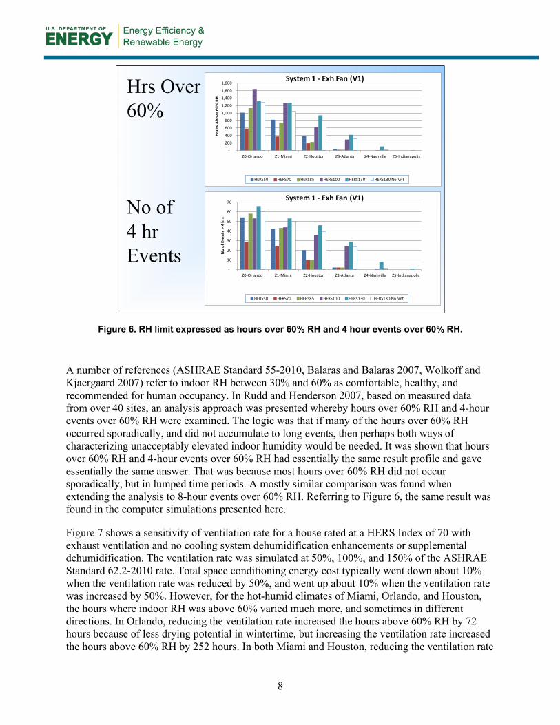
Figure 6. RH limit expressed as hours over 60% RH and 4 hour events over 60% RH.

A number of references (ASHRAE Standard 55-2010, Balaras and Balaras 2007, Wolkoff and Kjaergaard 2007) refer to indoor RH between 30% and 60% as comfortable, healthy, and recommended for human occupancy. In Rudd and Henderson 2007, based on measured data from over 40 sites, an analysis approach was presented whereby hours over 60% RH and 4-hour events over 60% RH were examined. The logic was that if many of the hours over 60% RH occurred sporadically, and did not accumulate to long events, then perhaps both ways of characterizing unacceptably elevated indoor humidity would be needed. It was shown that hours over 60% RH and 4-hour events over 60% RH had essentially the same result profile and gave essentially the same answer. That was because most hours over 60% RH did not occur sporadically, but in lumped time periods. A mostly similar comparison was found when extending the analysis to 8-hour events over 60% RH. Referring to Figure 6, the same result was found in the computer simulations presented here.

Figure 7 shows a sensitivity of ventilation rate for a house rated at a HERS Index of 70 with exhaust ventilation and no cooling system dehumidification enhancements or supplemental dehumidification. The ventilation rate was simulated at 50%, 100%, and 150% of the ASHRAE Standard 62.2-2010 rate. Total space conditioning energy cost typically went down about 10% when the ventilation rate was reduced by 50%, and went up about 10% when the ventilation rate was increased by 50%. However, for the hot-humid climates of Miami, Orlando, and Houston, the hours where indoor RH was above 60% varied much more, and sometimes in different directions. In Orlando, reducing the ventilation rate increased the hours above 60% RH by 72 hours because of less drying potential in wintertime, but increasing the ventilation rate increased the hours above 60% RH by 252 hours. In both Miami and Houston, reducing the ventilation rate

9

reduced the hours above 60% RH by 63% and 23%, respectively, and increasing the ventilation rate increased the hours above 60% RH by 76% and 35%, respectively.

Impact of Ventilation Rate HERS70

Exh Vent Hours Above

60% RH

AC Runtime

(hrs) AC EER (Btu/Wh)

AC Energy

(kWh)

Htg Energy

(kWh)

AHU Fan Energy

(kWh)

Exh Fan

Energy (kWh)

HRV Energy

(kWh)

Total Electric w/o HT

(kWh)

Total Costs w

Furnace ($)

50% Vent 678 1,774 16.6 3,093 554 594 91 - 3,778 419 91%100% Vent 606 1,851 16.7 3,270 686 622 203 - 4,095 460 100%150% Vent 858 1,915 16.8 3,419 862 646 305 - 4,370 500 109%

50% Vent 159 2,981 16.6 4,181 25 783 91 - 5,055 512 93%100% Vent 433 3,122 16.7 4,430 42 820 203 - 5,453 554 100%150% Vent 763 3,247 16.7 4,647 55 853 305 - 5,805 590 107%

50% Vent 164 2,307 16.3 3,241 1,792 635 91 - 3,967 411 92%100% Vent 214 2,391 16.4 3,403 2,045 661 203 - 4,267 446 100%150% Vent 288 2,461 16.5 3,537 2,522 687 305 - 4,529 488 109%

50% Vent 27 1,525 16.5 2,098 4,126 468 91 - 2,657 512 91%100% Vent 15 1,558 16.6 2,167 4,612 485 203 - 2,855 560 100%150% Vent 40 1,577 16.6 2,214 5,251 500 305 - 3,019 614 110%

Orlando

Miami

Houston

Atlanta

Figure 7. Impact of exhaust ventilation rate at 50%, 100% and 150% of the ASHRAE Standard 62.2-2010 whole-building ventilation rate.

A sensitivity comparing a conventional cooling system in a HERS 70 level house with cooling systems modified to increase latent capacity and a 50% RH setpoint is shown in Figure 8.

Enhanced AC represents three degrees of overcooling and lowered airflow (210 cfm/ton vs. 375 cfm/ton). This showed a reduction in hours over 60% RH of about 95% in Miami, 75% in Houston, and 50% in Orlando. However, field experience has shown that three degrees of overcooling (cooling to three degrees below the requested setpoint) causes comfort complaints. Note that the total space conditioning system operating cost is not directly comparable between the conventional system and the enhanced system because the enhanced system was modeled with a more efficient cooling system, as typically dictated in the market for systems with variable airflow.

Heat pipes (passive system for pre-cooling air entering the evaporator and reheating air leaving the evaporator) show a reduction in hours over 60% RH of about 90% in Miami, 60% in Houston, and 30% in Orlando. Due to the increased static pressure and associated increase in fan energy consumption associated with the heat pipe system, the total space conditioning system energy consumption and operating cost increased by 20%-25%.

10

With an indoor RH setpoint of 50%, the Humiditrol system by Lennox (employing overcooling by three degrees and refrigerant subcooling reheat) was able to control indoor RH below 60% in Miami and Houston, but still showed 32 hours above 60% RH in Orlando. Those hours occurred when overcooling had reached its limit.

Enhanced SystemsHERS70

Hours Above

60% RH

AC Runtime

(hrs) AC EER (Btu/Wh)

AC Energy

(kWh)

Htg Energy

(kWh)

AHU Fan Energy

(kWh)

Exh Fan Energy

(kWh)

Total Electric w/o HT

(kWh)

Total Costs w

Furnace ($)

Conv AC 606 1,851 16.7 3,270 686 622 203 4,095 460 Enhanced AC 308 3,826 20.8 2,756 699 196 203 3,155 366

AC w/ HPs 418 2,311 16.0 3,799 689 1,126 203 5,128 565 Lennox Humiditrol 32 4,000 17.0 3,374 703 265 203 3,843 436

Conv AC 433 3,122 16.7 4,430 42 820 203 5,453 554 Enhanced AC 20 5,721 19.9 3,772 48 339 203 4,315 439

AC w/ HPs 46 3,846 16.0 5,064 42 1,482 203 6,749 685 Lennox Humiditrol - 5,686 16.9 4,413 42 432 203 5,048 513

Conv AC 214 2,391 16.4 3,403 2,045 661 203 4,267 446 Enhanced AC 53 4,016 19.3 2,914 2,045 342 203 3,459 378

AC w/ HPs 93 2,918 15.9 3,837 2,044 1,157 203 5,197 525 Lennox Humiditrol - 4,061 17.3 3,233 2,039 380 203 3,817 408

Conv AC 15 1,558 16.6 2,167 4,612 485 203 2,855 560 Enhanced AC 15 2,619 19.7 1,819 4,594 270 203 2,292 501

AC w/ HPsLennox Humiditrol - 2,662 19.2 1,879 4,595 274 203 2,356 508

Miami

Houston

Atlanta

Orlando

Figure 8. Simulation results for enhanced Systems modeled in HERS 70 level houses.

11

Turn off capacitance, Check Gains

0.000 0.005 0.010 0.015 0.020Outdoor Humidity (lb/lb)

0.000

0.005

0.010

0.015

0.020

Indo

or H

umid

ity (l

b/lb

)

∆w = Qinternal = 0.33 lb/h ρ x 60 x cfm 0.075 x 60 x 58 cfm

Figure 9. A check of the simulation response with moisture capacitance turned off (set to zero).

Figure 9 provides a graphical check of the expected moisture modeling result with moisture capacitance turned off (set to zero). All values to the right of the solid line represent hours where moisture was being removed from the indoor air by the cooling system. All values between the dotted and solid lines represent hours where cooling was not active and internal moisture generation pushed the indoor humidity up beyond the outdoor humidity. If there was only ventilation and no internal moisture generation, the values would follow the solid line. Values to the left of the dotted line would be indicative of moisture capacitance, as shown in Figure 10 with measured and simulated indoor vs. outdoor humidity trends with indoor moisture capacitance.

A graphic illustration of the impact of overcooling is shown in Figure 11. Comparing the two plots, one can see how overcooling by three degrees moves or “sweeps” the higher RH hours down and to the left.

12

Comparing Humidity Trends

2010

0.000 0.005 0.010 0.015 0.020 0.025Outdoor Humidity (lb/lb)

0.000

0.005

0.010

0.015

0.020

0.025

Indo

or H

umid

ity (l

b/lb

)

0.000 0.005 0.010 0.015 0.020 0.025Outdoor Humidity (lb/lb)

0.000

0.005

0.010

0.015

0.020

0.025

Indo

or H

umid

ity (l

b/lb

)

Measured Simulated

∆w ~ 0.002 lb/lb

Figure 10. Measured and simulated indoor vs. outdoor humidity trends with indoor moisture capacitance.

Space ConditionsDaily Indoor Space Conditions: z1h100s1rh50v1

60 65 70 75 80 85 90Dry Bulb Temperature (F)

0.000

0.005

0.010

0.015

0.020

0.025

Hum

idity

Ratio

(lb/

lb)

40% 50% 60% 70% 80%

Hours Above 50% = 5361Hours Above 55% = 2399Hours Above 60% = 1303Hours Above 65% = 543Hours Above 70% = 107All HrsCooling Hrs

Impact of Overcooling (S2) in Miami

Figure 11. The impact of overcooling by three degrees “sweeps” the higher RH hours down and to the left.

Locating the air distribution system ducts inside conditioned space saves energy overall, but, with the reduced sensible cooling load, also comes an increased need for supplemental dehumidification. This impact is illustrated in Figure 12, where ducts in the attic were modeled

13

with 5% leakage (60% supply side, 40% return side). For the HERS 70 and HERS 50 efficiency levels, moving the ducts inside conditioned space increases the hours above 60% RH indoors by 25%-50%. A point of discussion in the meeting was that this difference may not be so large if the model were to account for the moisture desorption from wood framing materials that typically increase the attic humidity ratio over that of the outdoors during the late morning to early afternoon hours in warm-humid climates. In that case, return duct leakage would increase the moisture source for the ducts-in-attic configuration. This will be addressed in a simplified way by running an additional sensitivity with the attic dewpoint temperature being forced to 10oF over outdoors from 10 am to 1 pm between May 15 and October 15. However, this may not change the result that much since examining Figure 13 shows that, in Miami, for example, most elevated indoor RH hours occur in night and morning hours between late November and March. Some nighttime and rainy periods during mild summer conditions also produce elevated indoor RH.

Location of Ducts

-

200

400

600

800

1,000

1,200


Ho

urs

Ab

ove

60

% R

H

Location of Ducts

In Attic In Space In Attic In SpaceHERS 50 HERS 70

Figure 12. Locating the air distribution system ducts inside conditioned space saves overall energy, but also increases the need for supplemental dehumidification.

14

Shade Plot of Humidity Bins

z1h100s1rh50v1

Day (MAX/MIN = 5.00/ 0.00 )

Jan Feb Mar Apr May Jun Jul Aug Sep Oct Nov Dec2006

0

2

4

6

8

10

12

14

16

18

20

22

24

Hour

of Da

y

Shades of Gray

0 – below 55% 1 – 55-60% 2 – 60-65% 3 – 65-70% 4 – 75-80% 5 – above 80%

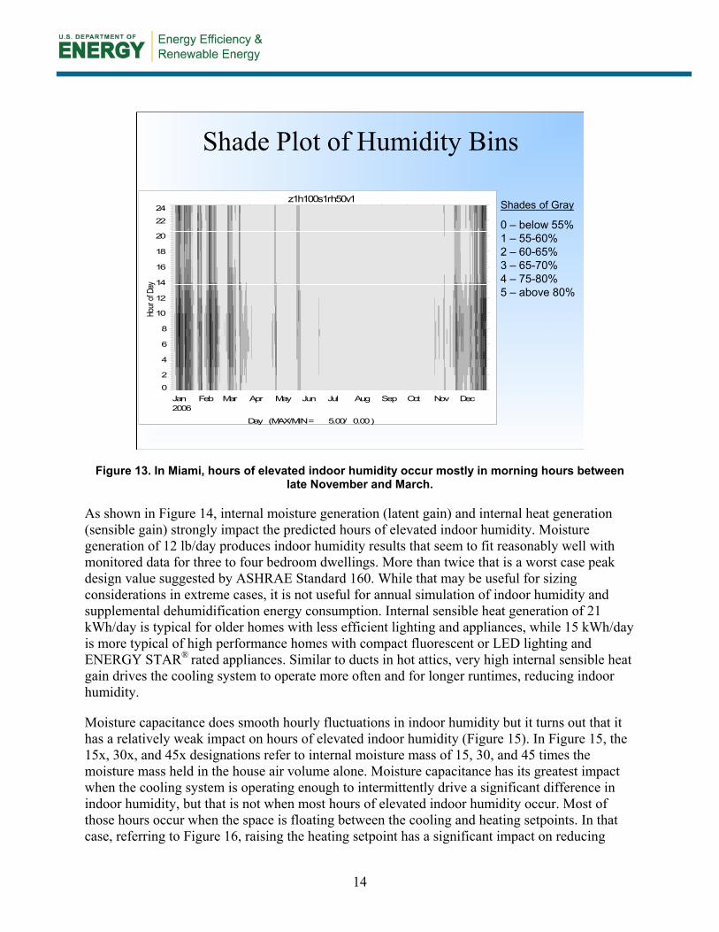
Figure 13. In Miami, hours of elevated indoor humidity occur mostly in morning hours between late November and March.

As shown in Figure 14, internal moisture generation (latent gain) and internal heat generation (sensible gain) strongly impact the predicted hours of elevated indoor humidity. Moisture generation of 12 lb/day produces indoor humidity results that seem to fit reasonably well with monitored data for three to four bedroom dwellings. More than twice that is a worst case peak design value suggested by ASHRAE Standard 160. While that may be useful for sizing considerations in extreme cases, it is not useful for annual simulation of indoor humidity and supplemental dehumidification energy consumption. Internal sensible heat generation of 21 kWh/day is typical for older homes with less efficient lighting and appliances, while 15 kWh/day is more typical of high performance homes with compact fluorescent or LED lighting and ENERGY STAR® rated appliances. Similar to ducts in hot attics, very high internal sensible heat gain drives the cooling system to operate more often and for longer runtimes, reducing indoor humidity.

Moisture capacitance does smooth hourly fluctuations in indoor humidity but it turns out that it has a relatively weak impact on hours of elevated indoor humidity (Figure 15). In Figure 15, the 15x, 30x, and 45x designations refer to internal moisture mass of 15, 30, and 45 times the moisture mass held in the house air volume alone. Moisture capacitance has its greatest impact when the cooling system is operating enough to intermittently drive a significant difference in indoor humidity, but that is not when most hours of elevated indoor humidity occur. Most of those hours occur when the space is floating between the cooling and heating setpoints. In that case, referring to Figure 16, raising the heating setpoint has a significant impact on reducing

15

indoor RH (even though it does nothing to reduce the absolute humidity) because it keeps the air from getting as cold, stopping the rise in RH.

Moisture & Sensible Gains

-

500

1,000

1,500

2,000

2,500

3,000

3,500

10.7 kWh/day 21.3 kWh/day 32 kWh/day

Hour

s Ab

ove

60%

RH

Orlando: Moisture & Sensible Gains

6 lb/day 12 lb/day 18 lb/day 24 lb/day

Figure 14. Hours of elevated indoor humidity is strongly related to internal moisture gains and internal sensible gains.

Moisture Gains & Capacitance

-

500

1,000

1,500

2,000

2,500

3,000

3,500

15x 30x 45x

Hour

s Ab

ove

60%

RH

Orlando: Moisture Gains & Capacitance

6 lb/day 12 lb/day 18 lb/day 24 lb/day

Figure 15. Hours of elevated indoor humidity is weakly related to moisture capacitance.

16

Sensible & Heating Set Pts

-

500

1,000

1,500

2,000

2,500

3,000

10.7 kWh/day 21.3 kWh/day 32 kWh/day

Hour

s Ab

ove

60%

RH

Orlando: Sensible Gains & Htg Set Pts

70F 72F 74F

Figure 16. Hours of elevated indoor humidity is strongly related to heating setpoint.

Figure 17 shows how these data are being made available on the Internet via an interactive web application where the user can choose simulation inputs and outputs to suit a particular interest.

Web Access to Resultscloud.cdhenergy.com/rp1449

Figure 17. Interactive Internet access is made available to retrieve customized sets of the simulation data.

17

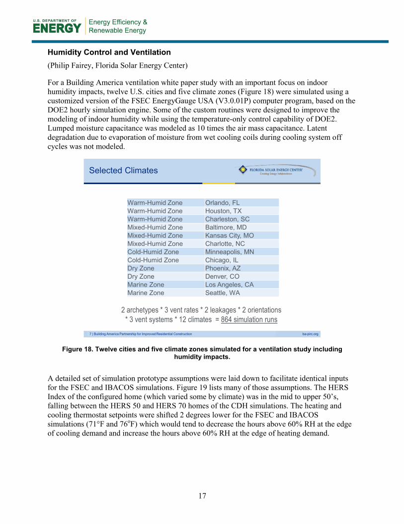
Humidity Control and Ventilation (Philip Fairey, Florida Solar Energy Center)

For a Building America ventilation white paper study with an important focus on indoor humidity impacts, twelve U.S. cities and five climate zones (Figure 18) were simulated using a customized version of the FSEC EnergyGauge USA (V3.0.01P) computer program, based on the DOE2 hourly simulation engine. Some of the custom routines were designed to improve the modeling of indoor humidity while using the temperature-only control capability of DOE2. Lumped moisture capacitance was modeled as 10 times the air mass capacitance. Latent degradation due to evaporation of moisture from wet cooling coils during cooling system off cycles was not modeled.

7 | Building America Partnership for Improved Residential Construction ba-pirc.org

Warm-Humid Zone Orlando, FLWarm-Humid Zone Houston, TXWarm-Humid Zone Charleston, SCMixed-Humid Zone Baltimore, MDMixed-Humid Zone Kansas City, MOMixed-Humid Zone Charlotte, NCCold-Humid Zone Minneapolis, MNCold-Humid Zone Chicago, ILDry Zone Phoenix, AZDry Zone Denver, COMarine Zone Los Angeles, CAMarine Zone Seattle, WA

Selected Climates

2 archetypes * 3 vent rates * 2 leakages * 2 orientations * 3 vent systems * 12 climates = 864 simulation runs

Figure 18. Twelve cities and five climate zones simulated for a ventilation study including humidity impacts.

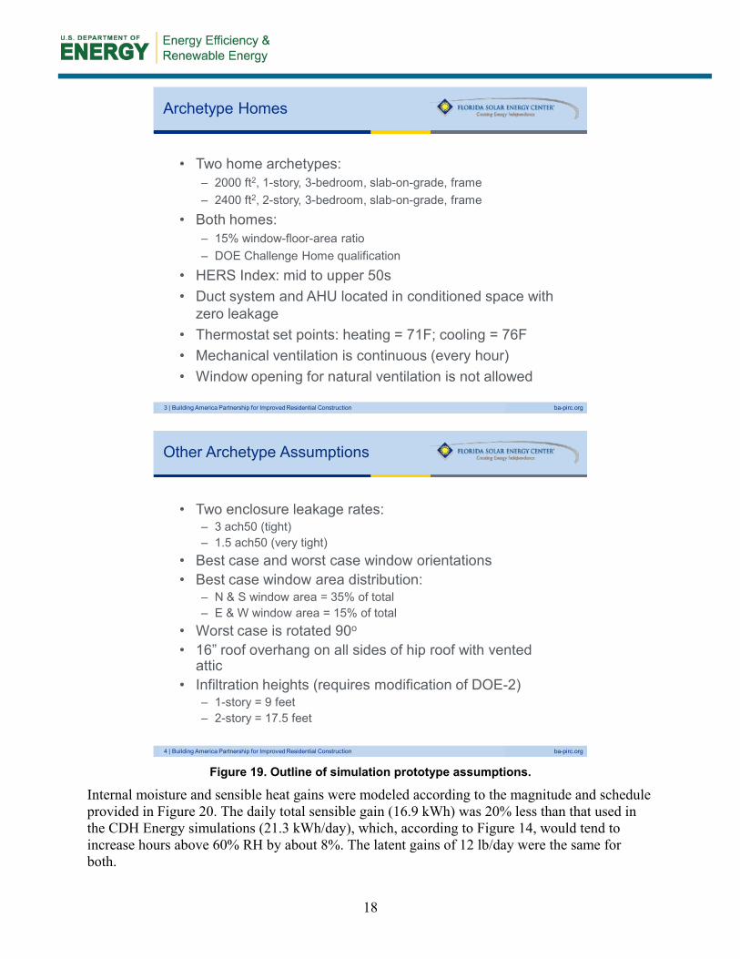
A detailed set of simulation prototype assumptions were laid down to facilitate identical inputs for the FSEC and IBACOS simulations. Figure 19 lists many of those assumptions. The HERS Index of the configured home (which varied some by climate) was in the mid to upper 50’s, falling between the HERS 50 and HERS 70 homes of the CDH simulations. The heating and cooling thermostat setpoints were shifted 2 degrees lower for the FSEC and IBACOS simulations (71°F and 76oF) which would tend to decrease the hours above 60% RH at the edge of cooling demand and increase the hours above 60% RH at the edge of heating demand.

18


• Two home archetypes:– 2000 ft2, 1-story, 3-bedroom, slab-on-grade, frame – 2400 ft2, 2-story, 3-bedroom, slab-on-grade, frame

• Both homes:– 15% window-floor-area ratio – DOE Challenge Home qualification

• HERS Index: mid to upper 50s• Duct system and AHU located in conditioned space with

zero leakage• Thermostat set points: heating = 71F; cooling = 76F• Mechanical ventilation is continuous (every hour)• Window opening for natural ventilation is not allowed

Archetype Homes


• Two enclosure leakage rates:– 3 ach50 (tight)– 1.5 ach50 (very tight)

• Best case and worst case window orientations• Best case window area distribution:

– N & S window area = 35% of total– E & W window area = 15% of total

• Worst case is rotated 90o

• 16” roof overhang on all sides of hip roof with vented attic

• Infiltration heights (requires modification of DOE-2)– 1-story = 9 feet– 2-story = 17.5 feet

Other Archetype Assumptions

Figure 19. Outline of simulation prototype assumptions.

Internal moisture and sensible heat gains were modeled according to the magnitude and schedule provided in Figure 20. The daily total sensible gain (16.9 kWh) was 20% less than that used in the CDH Energy simulations (21.3 kWh/day), which, according to Figure 14, would tend to increase hours above 60% RH by about 8%. The latent gains of 12 lb/day were the same for both.

19


Internal Gains Schedule

57,717 Btu sensible gains + 12,698 Btu (12.09 lb) latent gains

Figure 20. Internal sensible (16.9 kWh/day) and latent gains schedule used in the simulations.

Figure 22 shows analysis of simulation results for exhaust and ERV ventilation in Orlando. The hours above 60% RH are hours where the RH was above 60%. They are distinguished by heating, cooling, and floating hours. A heating hour was where any heating occurred during that hour, a cooling hour was where any cooling occurred during that hour, and a floating hour was an hour where no heating or cooling occurred during that hour. In an hour where both heating and cooling occurred, the one with the greater runtime was designated. The simulation assumed that the windows were closed and the space conditioning system was used all year.

As shown in Figure 22, most of the hours significantly above 60% RH occur during floating hours, which occur during fall, winter, and spring in Orlando. The ERV nearly eliminated the cooling hours above 60% RH, but it had little effect on the floating hours above 60% RH. That is because the cooling system forces a greater absolute humidity difference between the indoors and outdoors, which makes the ERV transfer more moisture to the exhaust stream. However, even though the ERV was modeled with a constant 60% effectiveness, meaning that 60% of the moisture from the higher absolute humidity side would be transferred to the lower absolute humidity side, 60% of a small absolute humidity difference is still a small amount of moisture. In other words, the ERV is ineffective in keeping indoor RH down during floating hours when the difference between indoor and outdoor absolute humidity is small.

20


Cooling Load and RH

Figure 21. For a week at the end of June and beginning of July on Orlando, the cooling system and space RH is showing an expected response.


Orlando: Exhaust vs. ERV

Figure 22. Hours above 60% RH for exhaust and ERV ventilation in Orlando.

21


Seasonal Impacts

HVAC condition for hours above 60% is strong function of climate

Figure 23. Hours above 60% by climate and space conditioning mode.

The hours above 60% RH during a particular space conditioning mode (heating, cooling, floating) was a strong function of climate. Figure 23 shows that the hours above 60% RH during heating are below 200 in every climate, but the hours above 60% RH while floating can be equal to or significantly greater than the hours above 60% RH during cooling and that is very dependent on the climate. For example, in Orlando, the hours above 60% RH are nearly equal between cooling hours and floating hours, but in Charleston and Houston, the hours above 60% RH are 35% to 50% greater for floating hours. However, the cooling hours above 60% RH are generally less than 65% RH while, in the warm-humid climates, the floating hours above 60% RH are generally in the range of 65% to 75% RH.

Figure 24 shows that, the hours of elevated indoor RH is a strong function of the selected RH limit and climate. For example, in Los Angeles, nearly all of the hours above 60% RH are also below 65% RH, but that is not true for Charleston, Houston, and Orlando.

Referring to Figure 25, mechanical ventilation, operated at the ASHRAE 62.2-2010 addendum r rate, in a 3 ach50 house, raises the annual median indoor RH by almost 10% RH compared to a 7 ach50 house without mechanical ventilation in Orlando. That is because infiltration drivers are generally weak in that climate during floating hours (when it is still humid outside and the cooling system is not removing moisture), but mechanical ventilation forces a minimum air exchange. Note that most of the RH increase due to ventilation is between 60%-65% RH; the hours between 65%-75% RH mostly remain the same. This indicates that some supplemental dehumidification would be needed in either case anyway.

22


Climate Severity

Climate Severity is a function of selected RH limit

Figure 24. Hours of elevated indoor RH is a strong function of the selected RH limit and climate.


2009 IECC Envelope Leakage

ASHRAE 62.2 exhaust ventilation raises median RH almost 10%

Internal gains: 57,717 Btu/day + 12.09 lb H2O/day

Figure 25. ASHRAE 62.2-2010 addendum r ventilation rate raises median RH compared to conventional dwelling without mechanical ventilation.

23


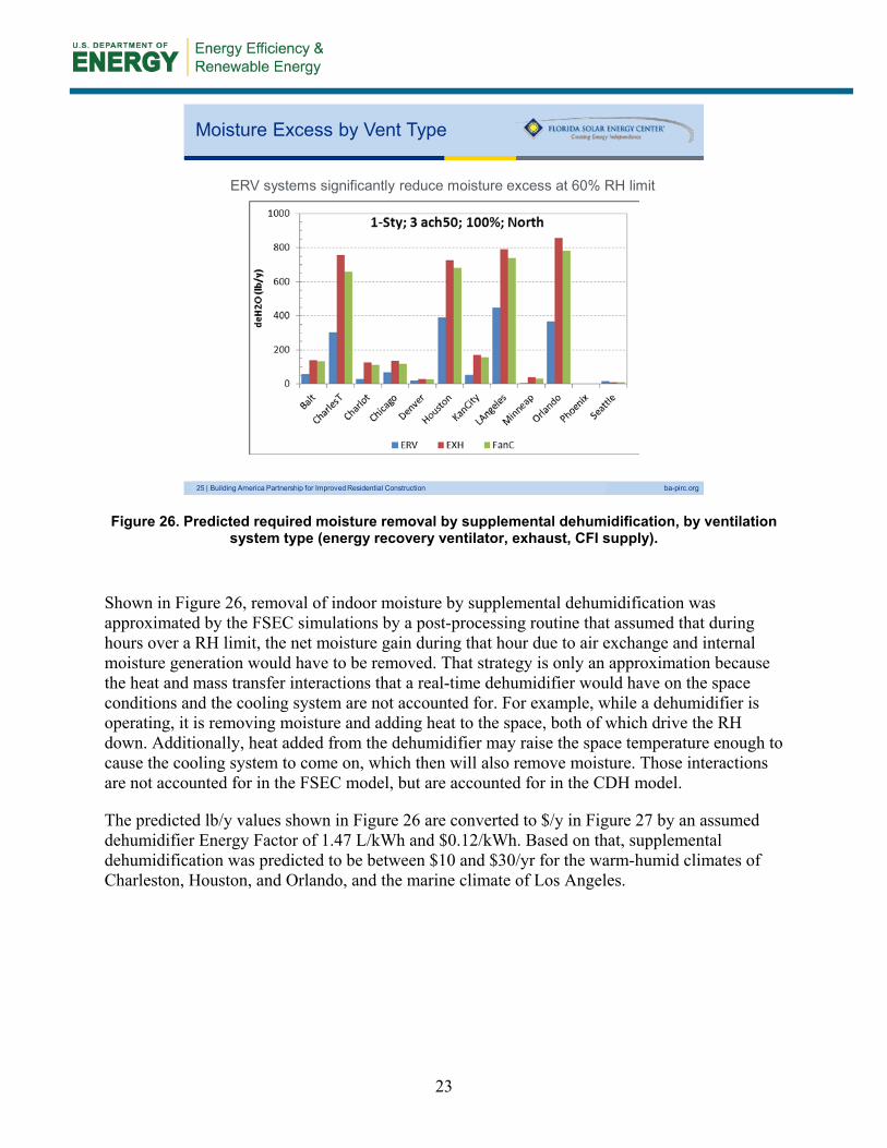
Moisture Excess by Vent Type

ERV systems significantly reduce moisture excess at 60% RH limit

Figure 26. Predicted required moisture removal by supplemental dehumidification, by ventilation system type (energy recovery ventilator, exhaust, CFI supply).

Shown in Figure 26, removal of indoor moisture by supplemental dehumidification was approximated by the FSEC simulations by a post-processing routine that assumed that during hours over a RH limit, the net moisture gain during that hour due to air exchange and internal moisture generation would have to be removed. That strategy is only an approximation because the heat and mass transfer interactions that a real-time dehumidifier would have on the space conditions and the cooling system are not accounted for. For example, while a dehumidifier is operating, it is removing moisture and adding heat to the space, both of which drive the RH down. Additionally, heat added from the dehumidifier may raise the space temperature enough to cause the cooling system to come on, which then will also remove moisture. Those interactions are not accounted for in the FSEC model, but are accounted for in the CDH model.

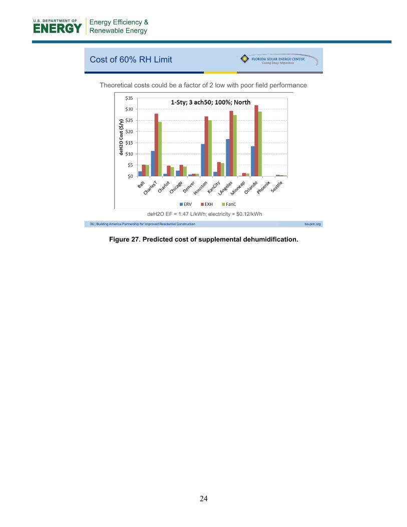
The predicted lb/y values shown in Figure 26 are converted to $/y in Figure 27 by an assumed dehumidifier Energy Factor of 1.47 L/kWh and $0.12/kWh. Based on that, supplemental dehumidification was predicted to be between $10 and $30/yr for the warm-humid climates of Charleston, Houston, and Orlando, and the marine climate of Los Angeles.

24


Cost of 60% RH Limit

deH2O EF = 1.47 L/kWh; electricity = $0.12/kWh

Theoretical costs could be a factor of 2 low with poor field performance

Figure 27. Predicted cost of supplemental dehumidification.

25

EnergyPlus Humidity Control and Ventilation Modeling Analysis (Michael Sypolt and Duncan Prahl, IBACOS)

IBACOS ran simulations in EnergyPlus that are parallel to those that FSEC ran in the customized version of EnergyGaugeUSA. The NREL BEopt E+ program was used to generate the geometry and base IDF files. A custom script modified parameters for about 860 runs which could be run overnight.

Figure 28. NREL BEopt E+ program used to generate the building geometry and the base IDF files (input description).

The model results were compared to the FSEC model results, and some input differences were corrected. Some result differences still exist. The EnergyPlus results generally show a greater number of hours over 60% RH indoors, and hours that extend to higher RH, compared to the FSEC (see Figure 29) and CDH simulations, and compared to much of BSC field data (Rudd et al. 2003, BSC 2004, Rudd et al. 2005). These might be due to differences in the infiltration model, or the infiltration-ventilation superposition. There may also be differences in the thermal energy balance model, which could lead to different loads, as another possibility. The EnergyPlus moisture modeling inputs were double checked by IBACOS and re-checked by FSEC without finding any significant discrepancies. The lumped moisture capacitance factor and moisture generation rate were consistent with the FSEC and CDH inputs.

26

Figure 29. Indoor RH vs. hour of year comparison between EnergyPlusPlus (blue symbols) and EnergyGauge USA (V3.0.01P) simulation results.

Figure 30, shows the energy consumption results by ventilation system type, ventilation rate, and building enclosure tightness. EnergyPlus shows the differences to be relatively small in each case.

Referring to Figure 31, using the IBACOS EnergyPlus model, an ERV (not integrated with the central AHU) reduces the number of hours with lowest and highest indoor RH in Orlando. Overall, there is a reduction in indoor RH, and a very large reduction in hours above 60% RH compared to the FSEC (not integrated with the central AHU) and CDH (integrated with the central AHU) models. This result is suspect, but the cause is unclear. In each case, the ERV moisture performance was modeled pretty simply as a constant effectiveness value applied to the actual indoor to outdoor humidity ratio difference. Of the three, the CDH model shows the highest hours above 60% RH because the ERV was configured as being connected between the return and supply of the central AHU, as most ERVs are installed. That installation configuration requires the AHU fan to operate coincident with the ERV fan (in this case a 50% duty cycle), which increased energy consumption and moisture evaporation when the cooling coil was wet. The CDH model calculates the amount of water retained on the cooling coil as a function of cooling runtime. Then, it calculates coil moisture evaporation starting each time the compressor

0

10

20

30

40

50

60

70

80

90

100

0 1000 2000 3000 4000 5000 6000 7000 8000

Houston Exhaust 100% ASHRAE

EG (V3.0.01P)

EnergyPlus

27

stops, and when the fan runs without the compressor. The FSEC and IBACOS models configured the ERV as separately ducted from the central air distribution system, and did not model coil moisture evaporation when the compressor was off.

Figure 30. Energy consumption results by ventilation system type, ventilation rate, and building enclosure tightness.

28

Figure 31. An ERV reduces the number of hours with lowest and highest indoor RH, and a very large reduction in hours above 60% RH compared to the FSEC and CDH models.

Analysis was conducted to look at window condensation potential and how that could impact a selected indoor RH limit from a durability perspective. Previous research (Arena et al. 2010) reported the highest occurrence of visible mold or moisture damage was on or around windows and in bathrooms. The window that was modeled was standard double pane with vinyl frame. For that window in Orlando, indoor RH above 75% shows risk of center-of-glass window condensation, especially during hours when the space conditions were floating between the heating and cooling set points (Figure 32). With a less thermally efficient window frame (non-thermally broken aluminum is common in Florida due to high wind resistance requirements), a lower indoor RH threshold would be needed to avoid condensation on or near the window frame.

29

Figure 32. Window condensation potential during Orlando floating hours

7 Answers to Research Questions

• What are the important humidity control conclusions from recent residential dehumidification systems modeling, with a wide range of building and equipment sensitivity, using a customized <2 minute time-step TRNSYS model with temperature and humidity control?

o Internal moisture generation, internal sensible heat generation, heating setpoint temperature, and air distribution system duct location (inside or outside of conditioned space) are the major influencers of elevated indoor RH in high performance homes in warm-humid climates.

o Mechanical ventilation is a secondary factor in increasing hours above 60% RH.

o Moisture capacitance is a secondary factor, and lumped moisture mass factors of 10 to 30 times the air mass capacity do not show significant difference in indoor RH.

o Supplemental dehumidification by either a stand-alone dehumidifier, ducted dehumidifier, or gas-fired desiccant dehumidifier (e.g. NovelAire ComfortDry 400 in supply air stream) was effective in eliminating hours over 60% RH. In Orlando, Miami, and Houston, the difference in total HVAC operating cost between a HERS 70 level house with those systems was 15%, 11%, and 1%, respectively. The gas-fired desiccant system showed the lowest operating cost, followed by the ducted dehumidifier and the stand-alone dehumidifier.

o Cooling system enhancement by subcooling condenser reheat was effective in eliminating hours over 60% RH in Miami and Houston, and nearly so in Orlando.

30

o Heat pipe cooling system enhancement was less effective than three degrees overcooling plus low evaporator coil airflow (210 cfm/ton). Both were more effective in Miami and Houston than in Orlando, but even in Orlando the hours over 60% RH were reduced by about half (600 down to about 350 on average). However, questions remain as to whether the overcooling can be tolerated from a comfort perspective.

o Two-speed and variable speed cooling systems do not appreciably reduce hours above 60% RH unless coupled with lower than standard cooling airflow (cfm/ton).

• What are the important indoor humidity conclusions that can be drawn from recent residential ventilation modeling efforts using the temperature-only control logic of the FSEC EnergyGauge USA program?

o Most of the hours significantly above 60% RH occur during floating hours, which occur during fall, winter, and spring in Orlando.

o In Orlando, an ERV nearly eliminated the cooling hours above 60% RH, but it had little effect on the floating hours above 60% RH.

o Hours above 60% RH during a particular space conditioning mode (heating, cooling, floating) was a strong function of climate.

o Hours of elevated indoor RH is a strong function of the selected RH limit and climate. For example, in Los Angeles, nearly all of the hours above 60% RH are also below 65% RH, but that is not true for Charleston, Houston, and Orlando.

o Mechanical ventilation, operated at the ASHRAE 62.2-2010 addendum r rate (about 25% more than before addendum r), in a 3 ach50 house, raises the annual median indoor RH by almost 10% RH compared to a 7 ach50 house without mechanical ventilation in Orlando. However, most of the RH increase due to ventilation is between 60%-65% RH; the hours between 65%-75% RH mostly remain the same. This indicates that some supplemental dehumidification would be needed in either case anyway.

o Supplemental dehumidification was predicted to be between $10 and $30/yr for the warm-humid climates of Charleston, Houston, and Orlando, and the marine climate of Los Angeles. However a caveat was provided that indicates that this value is predicated on an operating dehumidifier EF of 1.47 L/kWh and recent field data indicates that conventional dehumidifiers operate closer to 0.8 L/kWh (Mattison and Korn 2012), which would tend to double this cost. Additionally, dehumidifiers tend to operate on a large humidity deadband, which means that maintaining humidity below 60% would likely require humidity setpoints near 55%, which would dramatically increase dehumidification costs.

31

• What are the important humidity control conclusions from recent residential ventilation modeling efforts using the temperature and humidity control logic of the Energy Plus version of the NREL BEopt program?

o Energy consumption by ventilation system type, ventilation rate, and building enclosure tightness showed relatively small differences in each case compared to total HVAC energy consumption.

o Durability analysis for Orlando, for a standard double pane window with vinyl frame, showed that indoor RH above 75% risks center-of-glass window condensation, especially during hours when the space conditions are floating between the heating and cooling set points. With a less thermally efficient metal window frame, the risk would be greater.

• How do the results from these different programs compare?

The most important way in which the results differ between the simulation programs is in the frequency and magnitude of elevated indoor RH. For example, in Orlando, the CDH, FSEC, and IBACOS results show hours above 60% RH in the range of 1000, 2000, and 3000, respectively. In terms of maximum indoor RH, the CDH and FSEC results both show about 75% while the IBACOS results show about 85%. However, in all cases, supplemental dehumidification would be required for high performance, low-energy houses, and the difference in supplemental dehumidification energy would probably be less than 150 kWh/yr or less than $20/yr.

The IBACOS ERV modeling using EnergyPlus is suspect of showing too much reduction in elevated indoor humidity hours compared to both the CDH and FSEC models, however, the CDH model did not model the ERV as a completely separate system from the central system ducts. After a sensitivity run by CDH is done with an ERV as a completely separate system, the results will be more directly comparable.

• Is it generally agreed that controlling to less than 60% RH is the appropriate humidity control point for high performance homes, and why?

It was generally agreed that, a dehumidification control setpoint of 55%, in order to keep indoor RH from exceeding a 60% RH limit, was the correct strategy for high performance, low-energy homes. While it is clear that everything will not fail at once if the indoor RH goes over 60%, a 60% RH limit provides the best practice coverage for providing comfort and durability over a reasonable range of varying factors, such as internal moisture generation rate, and occupant comfort perception and susceptibility to illness stemming from elevated indoor humidity. Included in the variability of internal moisture generation rate is construction moisture drying. It has been BSC’s experience that limiting indoor RH to 60% via supplemental dehumidification is a generic enough limit to remove moisture concerns related to the seasonal timing of building closure and occupancy in warm-humid climates.

• Is it generally agreed that annual hours above 60% RH is the appropriate humidity control performance metric to use to compare system performance and to compare

32

required supplemental dehumidification energy? Does that metric give generally the same result as looking at 4-hour and 8-hour events above 60% RH?

It was generally agreed that annual hours above 60% RH is the single most appropriate humidity control performance metric to use to compare system performance and to compare required supplemental dehumidification energy. That metric does give generally the same result as looking at 4-hour and 8-hour events above 60% RH.

• For a range of climates, ventilation systems, and space conditioning equipment in high performance homes, what is the magnitude of hours above 60% RH, the magnitude of supplemental dehumidification energy required to control to less than 60% RH, the time of year occurrence of elevated indoor humidity and supplemental dehumidification, and the space conditioning mode (heating, cooling, floating) during which most periods of elevated indoor humidity and supplemental dehumidification occur?

The answers to this question are given in more detail in section 6, Agenda Summaries, but are summarized here. The warm-humid climates of Miami, Orlando, Houston, and Charleston show a clear need for supplemental dehumidification for high performance homes. Without supplemental dehumidification, hours above 60% RH were in the range of 800 to 1800, with hours above 65% being about half of that. Most of the hours of elevated indoor humidity occur in the mild temperature but humid outdoor conditions of fall and spring, but also occur in winter in Orlando and Miami. A smaller number of hours occur during some summer nights and days-long rainy periods. Few hours above 60% RH occur during heating hours. Most hours between 60%-65% RH occur during either cooling or floating hours, and most hours above 65% RH occur during floating hours. The supplemental dehumidification energy consumed to keep indoor RH below 60%, taken as the difference in total HVAC cost for the same building with and without supplemental dehumidification, is relatively small. It is in the range of 250 kWh/yr or less ($30/yr or less), but necessary to enable deep cuts in sensible heat gain without incurring long periods of elevated indoor RH.

8 Action Items

The following action items were discussed at the end of the meeting:

• Continue to do more checking to understand the EnergyPlus moisture modeling differences compared to the FSEC and CDH modeling.

• Add a sensitivity run using the CDH model for an ERV not integrated with the central air distribution system.

• Add a sensitivity run using the CDH model to further detail the difference between ducts in the attic and ducts in the conditioned space, where the attic dew point temperature is increased 10oF between 10 am and 1 pm between May 15 and October 15.

33

• Contact Association of Home Appliance Manufacturers (AHAM) to explore the prospect of developing a new residential dehumidifier standard encompassing two test points in addition to the one test point in their existing standard, and reporting of additional test results.

o From discussion of Figure 33, the group proposed a new dehumidifier test condition of 75oF and 55% RH to represent spring/fall part load cooling conditions, and a new test condition of 65oF and 50% RH to represent basement conditions where avoiding high RH or condensation on cool below-grade concrete walls and floors is needed. These new test conditions could replace the AHAM test conditions or could be in addition to the legacy test condition of 80oF and 60% RH in the current AHAM standard if considered necessary on a consensus basis, primarily as a transitional measure for comparison to legacy test results. The AHAM test point of 80°F/60% RH is not a common indoor environmental condition for occupied spaces, limiting its usefulness to consumers and designers. Thermodynamics dictate that for the same RH set point, dehumidifier energy consumption will be higher at lower, more common indoor dry-bulb temperatures. NREL reported performance maps of several dehumidifiers at various operating conditions (Winkler et al. 2011).

Figure 33. Overview of recommended dehumidifier test conditions.

Indoor Sensible Latent Moisture MoistureInlet Outlet Wet-coil Cooling Cooling Removal Total Removal

T/RH/Tdp T/RH/Tdp Airflow Capacity1 Capacity Capacity Power Efficiency2

Test condition represents: (F/%/F) (F/%/F) (cfm) (Btu/h) (Btu/h) (L/h) (kW) (L/kW-h)

Current AHAM test Test 1 80/60/65Sping/Fall part load cooling3 Test 2 75/55/58Basement Test 3 65/50/46

1 Negative cooling capacity denotes net heat added from inlet to outlet2 Same units as the USDOE and USEPA Energy Factor for dehumidifiers3 All tests with steady wet coil

34

9 References

ANSI/AHAM DH-1-1992, (Reaffirmation of DH-1-1986), “Dehumidifiers.” The Association of Home Appliance Manufacturers' Approved as an American National Standard. March 25, 1992. Published by Association of Home Appliance Manufacturers, 1111 19th Street, NW Suite 402, Washington, DC 20036, 202/872-5955. ASHRAE Standard 160-2009, Criteria for Moisture-Control Design Analysis in Buildings. ANSI/ASHRAE Standard 55-2010, Thermal Environmental Conditions for Human Occupancy. Arena, L. B.; Karagiozis, A.; Mantha, P. (2010). “Monitoring of Internal Moisture Loads in Residential Buildings - Research Findings in 3 Different Climate Zones.” Thermal Performance of the Exterior Envelopes of Whole Buildings XI, Clearwater Beach, Florida, December. BETEC, ASHRAE, ORNL. Balaras, C.A. (2007). "HVAC and indoor thermal conditions in hospital operating rooms". Energy and Buildings 39 (4): 454. BSC (2004). “Results of Advanced Systems Research, Deliverable Number 5.C.1” Project 3 – Supplemental Humidity Control Systems, pg. 8-10 of Final Report to U.S. Dept. of Energy under Task Order No. KAAX-3-32443-05 under Task Ordering Agreement No. KAAX-3-32443-00, pg. 8-10, October 29. Midwest Research Institute, National Renewable Energy Laboratory Division, Golden, CO. BSC (2006). “Systems Engineering Approach To Development Of Advanced Residential Buildings, 11.B.1 Results Of Advanced System Research.” Project 6 – Enhanced Dehumidifying Air Conditioner of Final Report to U.S. Dept. of Energy under Task Order No. Kaax-3-32443-00 under Task Ordering Agreement No. Kaax-3-32443-10. Midwest Research Institute, National Renewable Energy Laboratory Division, 1617 Cole Boulevard, Golden, CO. BSC (2007a). “Systems Engineering Approach To Development Of Advanced Residential Buildings, 14.B.1 Results Of Advanced Systems Research”, Project 1 – Enhanced Dehumidifying Air Conditioning of Final Report To U.S. Dept. of Energy under Task Order No. Kaax-3-32443-14 under Task Ordering Agreement No. Kaax-3-32443-00. Midwest Research Institute, National Renewable Energy Laboratory Division, 1617 Cole Boulevard, Golden, CO. BSC (2007b). “Whole House Ventilation System Options – Phase 1 Simulation Study.” ARTI Report No. 30090-01, Final Report, March. Air-Conditioning and Refrigeration Technology Institute, Arlington, VA. Henderson, H.I.; Rengarajan., K.; Shirey, D.B. (1992). “The Impact of Comfort Control on Air Conditioner Energy Use in Humid Climates”, ASHRAE Transactions Vol. 98 Part 2.

35

Henderson, H.; Shirey, D.; Raustad, R. (2007). “Development of a New Climate-Sensitive Air Conditioner (Task 4): Simulation Results and Cost Benefit Analysis”, FSEC-CR-1716-07, Cocoa: Florida Solar Energy Center. Henderson, H. and Rice, C.K. (2008). "Analysis of Dehumidification Options in Standard Practice and Near-Zero Energy Homes", Oak Ridge National Laboratory Report ORNL/TM-2008/64. Mattison, L. and Korn, D. (2012). “Dehumidifiers: A Major Consumer of Residential Electricity.” 2012 ACEEE Summer Study on Energy Efficiency in Buildings. American Council for an Energy Efficient Economy, Washington D.C. Rudd, A.; Lstiburek, J.; Ueno, K..(2003). “Residential dehumidification and ventilation systems research for hot-humid climates,” Proceedings of 24th AIVC and BETEC Conference, Ventilation, Humidity Control, and Energy, Washington, US, pp.355–60. 12-14 October. Air Infiltration and Ventilation Centre, Brussels, Belgium. Rudd, A.; Lstiburek, J.; Ueno, K. (2005). Residential dehumidification systems research for hot-humid climates. U.S. Department of Energy, Energy Efficiency and Renewable Energy, NREL/SR-550-36643. www.nrel.gov/docs/fy05osti/36643.pdf. Rudd, A.; Henderson, H.. (2007). “Monitored Indoor Moisture and Temperature Conditions in Humid Climate U.S. Residences.” ASHRAE Transactions (17, Dallas 2007). American Society of Heating Refrigeration and Air-Conditioning Engineers, Atlanta, GA. Shirey, D.B.; Henderson, H.I.; and Raustad, R. (2006). “Understanding the Dehumidification Performance of Air-Conditioning Equipment at Part-Load Conditions”, Final Report, FSEC-CR-1537-05, Cocoa: Florida Solar Energy Center. Winkler, J.; Christensen, D.; Tomerlin, J. (2011). “Laboratory Test Report for Six ENERGY STAR® Dehumidifiers.” Technical Report NREL/TP-5500-52791, National Renewable Energy Laboratory, Golden, CO. Wolkoff, S.and Kjaergaard, K. (2007). "The dichotomy of relative humidity on indoor air quality". Environment International 33 (6): 850.

DOE/GO-102013-3856 ▪ July 2013

Printed with a renewable-source ink on paper containing at least 50% wastepaper, including 10% post-consumer waste.

Expert Meeting: Recommended Approaches to · PDF fileExpert Meeting: Recommended Approaches to...

Documents

Transcript of Expert Meeting: Recommended Approaches to · PDF fileExpert Meeting: Recommended Approaches to...