Experiments with

Electricity and Magnetism

for

Physics 336L

by

R. Sonnenfeld

New Mexico Tech

Socorro, NM 87801

Copyright c©2013 by New Mexico Tech

January 23, 2013

i

Contents

Course schedule v

Course Goals 1

Safety 1

Required Supplies 2

Lab Reports 2

1 Circuits (n=1) 8Understand DC series and parallel circuits and light-bulbs . . . . . . . . . . . . . . . . . 8

2 Internal Impedance and Error Analysis (n=1) 15Measuring input impedance of a voltmeter and output impedance of a battery . . . . . 15

3 Complex Impedance (n=1) 18Measure complex impedance of a resistor and a capacitor . . . . . . . . . . . . . . . . . 18

4 Magnetic Field, Inductance, Mutual Inductance, and Resonance (n=2) 20Characterizing an LR circuit and determining impedance of an inductor with an oscil-

loscope and voltmeter . . . . . . . . . . . . . . . . . . . . . . . . . . . . . . . . . . 20

5 Hysteresis (n=2) 24Measure hysteresis loop of a soft iron torus and learn how a transformer works . . . . . 24

6 Diodes and Transistors (n=1) 31Characterize a diode, then build a one-transistor amplifier . . . . . . . . . . . . . . . . . 31

7 Operational Amplifiers (n=2) 34Learn basic op-amp theory then build an inverting and non-inverting op-amp . . . . . . 34

8 Automobile Circuits (n=1) 39I-V curve of a light bulb - High Voltage from an ignition coil – Analyze a blinker . . . . 39

9 Index of Refraction of Air (n=1) 40Compare optical path length in air to vacuum using an interferometer . . . . . . . . . . 40

10 Electric Field, Capacitance, Dielectric Constant (n=1) 41Use a capacitor to measure the dielectric constant of liquid nitrogen . . . . . . . . . . . 41

11 Negative Resistance (n=1) 42Measure I-V curve of neon lamp. Use negative resistance to create an oscillator . . . . . 42

12 Superconductivity (n=1) 43Understand Meissner effect with a High Tc superconductor . . . . . . . . . . . . . . . . 43

13 Serial Ports (n=1) 48Decode the signals that come out of a computer terminal. . . . . . . . . . . . . . . . . . 48

ii

14 Miscellaneous Experiments (n=various!) 51Develop an outlined experiment or create your own . . . . . . . . . . . . . . . . . . . . . . . . . . . . . . 5114.1 Design your own! . . . . . . . . . . . . . . . . . . . . . . . . . . . . . . . . . . . . . 51Concieve and develop your own experiment . . . . . . . . . . . . . . . . . . . . . . . . . . . . . . . . . 5114.2 Lock-in Amplifiers . . . . . . . . . . . . . . . . . . . . . . . . . . . . . . . . . . . . 51Lock-in amplifiers allow you to see a tiny signal in the presence of substantial noise . . . . . . . . . . . . . . . . . . 5114.3 TV remote control . . . . . . . . . . . . . . . . . . . . . . . . . . . . . . . . . . . . 51Detect and decode the infra-red control pulses sent by a TV remote . . . . . . . . . . . . . . . . . . . . . . . . 5114.4 Resistance and temperature . . . . . . . . . . . . . . . . . . . . . . . . . . . . . . . 51How does resistivity vary with temperature? . . . . . . . . . . . . . . . . . . . . . . . . . . . . . . . . . 5114.5 Electric Motors . . . . . . . . . . . . . . . . . . . . . . . . . . . . . . . . . . . . . . 52Electric motors can be used in reverse as electric generators . . . . . . . . . . . . . . . . . . . . . . . . . . . 5214.6 Magnetic materials . . . . . . . . . . . . . . . . . . . . . . . . . . . . . . . . . . . . 52Measure magnetic properties of materials by incorporating them in an inductor. . . . . . . . . . . . . . . . . . . . 5214.7 Electric and magnetic fields of a power line . . . . . . . . . . . . . . . . . . . . . . 52Figure out how to measure the E and/or B-field from a power line . . . . . . . . . . . . . . . . . . . . . . . . 5214.8 Flames . . . . . . . . . . . . . . . . . . . . . . . . . . . . . . . . . . . . . . . . . . . 52What are the electrical properties of flames? . . . . . . . . . . . . . . . . . . . . . . . . . . . . . . . . . 5214.9 Guitar Pickup . . . . . . . . . . . . . . . . . . . . . . . . . . . . . . . . . . . . . . 52How do electric guitar pickups work? . . . . . . . . . . . . . . . . . . . . . . . . . . . . . . . . . . . . 5214.10Build a rail gun . . . . . . . . . . . . . . . . . . . . . . . . . . . . . . . . . . . . . . 52Build a rail gun! Group project . . . . . . . . . . . . . . . . . . . . . . . . . . . . . . . . . . . . . . 5214.11Build an electromagnetic can crusher . . . . . . . . . . . . . . . . . . . . . . . . . . 52A pulsed magnetic field can cause a coke-can to crush itself via eddy curret . . . . . . . . . . . . . . . . . . . . . 52

Appendices 54

iii

Acknowledgments

A number of faculty and students at New Mexico have contributed to the experiments for thisjunior-level laboratory class. The ones I know about are:

Prof. Marx Brook,Prof. J. J. (Dan) Jones,Prof. Paul Krehbiel,Prof. Charles B. Moore,Prof. William Rison,Mr. Robert Rogers, andProf. William P. Winn

iv

2013 Course schedule

Date Lab Due

1/23 Circuits

1/30 Internal Imp. Examples/Writeup

2/06 Complex Imp. Int. Imp.

2/13 BLMR Complex

2/20 BLMR BLMR

2/27 Hysteresis BLMR

3/06 Break —

3/13 Hysteresis

3/20 Diodes Hysteresis

3/27 No Lab Diodes

4/03 OpAmps

4/10 OpAmps OpAmps

4/17 Option1 Opamps

4/24 Option2 Option1

5/1 Make-up Option2

5/8 Finals Make-Up

Table 1: This is the approximate schedule we will follow. Labs are due one week after they arecompleted. There is slack in the schedule for illness or other personal needs.

v

Introduction

Course Goals and Time Committment

There are four purposes for this course.

• To give practical examples of concepts learned in Phys333/334

• To let you experience some of the excitement (and confusion) of experimental physics.

• To give you a working comfort with basic electronics as it appears universally in a modernphysics lab.

• To somewhat enhance your abilities with data analysis and error propagation.

The labs vary in length, but will take at least two hours to get through and understand. The coursegrade is based on your lab reports and your level of effort in class. The individual measurementsyou are asked to do are not particularly time-consuming; that is intentional. The time you are notspending putting things together and making measurements is meant to be spent understandingyour results and how they fit the basic electromagnetic theory that you have learned to this pointin your career.

Depending on your level of understanding, it will require one to three hours after each classsession to complete the data analysis, perform the needed derivations, and do the backgroundreading to needed to understand your results.

References

The following references will be invaluable to you throughout your career if you do any kind ofexperimental work. They are not required, but if you choose to buy them now, you will likely notneed another reference for basic electronics or error analysis for at least a decade.

Horowitz, Paul, and Hill, Winfield, The Art of Electronics (2nd edition), Cambridge UniversityPress, New York City, 1989.

Taylor, John R., An Introduction to Error Analysis, 2nd Edition, University Science Books,Sausalito, California, 1997.

Safety

• Shoes and socks are required for minimal safety.

• Campus police are available at 835-5434 in case of emergency.

• Know the location of the nearest FIRE EXTINGUISHER. Can this fire extinguisher beused on electrical fires?

• Know the location of the nearest FIRE ALARM pull lever.

• Report defective or damaged equipment to the instructor.

• Construct experiments so they can not fall and so that people will not trip over wires.

• Do not energize any experiment using more than 30 V until the instructor has inspected it.

1

• Conventional lab protocol calls for no food or drink under any circumstances. I have loosenedthis ban because I have observed that science runs on caffeine. Thus, black coffee, tea, orbottled water are the only drinks allowed in the lab. Sugar and sweeteners are destructiveto electronics, and many drinks (e.g. Coca-Cola) are corrosive. In the event of a spill, youare responsible to promptly clean and dry any lab equipment involved. You may be requiredto dissassemble, dry, and retest your equipment if liquid has penetrated the case.

• Food and snacks are not permitted in the lab. If you are hungry, you can take a quick snackbreak out in the Workman lobby.

• One reason that labs usually ban food and drink is that hazardous chemicals (e.g. lead)are associated with electronics. Thus, you shall wash your hands between working with labequipment and eating.

Laboratory Protocol

• The Laboratory hours are 2 PM to 4:30 PM. Please arrive on time. Habitual late-ness/absence will affect your grade. If you finish an experiment early, begin working onyour analysis or on the next experiment.

• The lab has wireless internet connectivity. You may bring a lap-top to assist in data plot-ting/analysis or for web research related to your analysis.

• Please limit your conversations in the laboratory to the experiments.

• You are encouraged to help your fellow student learn the material, but all are responsiblefor their own understanding.

Required Supplies

Failure to bring the following supplies every time can result in grade reductions. (See section ongrading).

• This lab manual is obviously needed every class.

• A 3-ring binder for lab write-ups should be brought to every class. Some labs refer back toearlier labs. Even if you do your labs purely electronically, print previous labs out and putthem in the binder.

• A notebook for recording your data that includes data from earlier labs. This notebook maybe the same 3-ring binder mentioned above or a separate laboratory notebook. Do whatworks best for you.

• A calculator or computing device with a calculator built in. This allows you to do prelimi-nary data analysis in lab.

Lab Reports & Moodle

You can find this class on Moodle. There is a section for uploading your lab report. I would likeall reports to be submitted via Moodle. This may mean that you need to scan in hand-writtentables, sketches, and graphs include them in your report. To facilitate this, you probably wantto put these all together on a single sheet (or two) of paper. Then you only need to scan one or

2

two pages rather than several. (Cameras are alternatives to scanners, provided the final resultis readable). If you have the technology, and wish to create your graphs, sketches, and tablesdirectly in electronic form, this is of course acceptable.

I will provide on request LaTeX templates for a lab report if you already know or would liketo learn LaTeX. Inferior programs like Microsoft Word, or less inferior programs like Open-OfficeWriter are also acceptable. Open-Office can easily directly generate a .pdf from any file. Pleasedo not submit .docx or .odt files, only pdfs.

Your lab report shall be clear and legible. It may be typed, or hand-written directly in yourlab book and scanned to pdf. Your report should have the following sections:

1. Heading – In the following order, state

(a) Your name

(b) The name of the experiment

(c) Date the report was written.

(d) Date the laboratory work was finished.

2. Vocabulary – Define each word and state how it relates to the experiment.

3. Apparatus and Procedure –Describe what you did. Use figures to show how the equipment and circuits were hooked up.

For each piece of equipment you use, record (and report) the following:

(a) Description (e.g. voltmeter, oscilloscope)

(b) Manufacturer Model (e.g. HP 6235A)

(c) Serial number

Recording the Model and Serial numbers will help you get consistent results if you need tocontinue the same lab over one or more periods. This information will also be helpful shouldthe equipment become faulty and in need of repair.

4. Answers to Numbered Questions – Some labs are more formally structured than others.In labs where I have numbered the measurements you should report or the calculations youshould do, it is efficient for both of us to simply structure the rest of your report aroundreporting what you were asked to report and calculating/deriving what you were asked tocalculate or derive. In labs that are more free-form, you will want to continue with theorder as shown below. Even for labs with numbered questions, please read the sectionsbelow suggesting how to present raw data, calculations, and derivations.

5. Error Discussion – The next section of this manual explains formal error analysis. Inincludes a fancy expression with partial derivatives. This level of analysis is only requiredfor the lab called Internal Impedance. HOWEVER, a brief (couple of sentence) discussion oferrors is required in every lab (even those that mostly revolve around answering numberedquestions). Your discussion should specify what the error is in your raw measurementsand how your arrived at that number. You should also estimate the error in your derivedmeasurements.

3

6. Measured variables and data tables – The column headings of your data table shouldlist the name of the variable being measured and the units of the numbers contained. Intheoretical courses, variables often represent quantities like ~E or ~B or ǫ. In the laboratory,variables represent the number of divisions on an oscilloscope or the voltage on a voltmeter.An imprecise table would have a column headed “Voltage (V)”. A more precise table wouldindicate the part of the circuit the voltmeter was connected to. A well-defined variable couldbe called VAB, where A and B are the two points on your circuit to which the voltmeterprobes were applied. VAB would be further defined by the inclusion of the circuit diagramwith the table with A and B marked on it.

It is not unusual for the raw data taken by a physicist to be somewhat disorganized. (Thisvaries with the physicist!). For example, when measuring the amplitude of a resonant circuitvs. the frequency at which it is driven, one may take a number of data points that are nottoo interesting (because they are not near the resonance). You might also obtain data thatyou later decide are incorrect or ambiguous (because you forgot to note the scale of anoscilloscope, for example). Your notebook may thus contain a jumble of dubious data andgood data. For the lab report, you can recopy the data table in a well-ordered way. Feel freeto omit any dubious or redundant data points. Alternatively, do enough measurements tounderstand what constitutes a valid datum and what columns should be in a table. Then,draw a neat table and continue your experiment, completing the table as you go. You canthen scan the table and include it in your lab report without rewriting it.

7. Graphs – Show data as points (not lines) and theoretical curves as lines. Use computerplotting software, or plot by hand in your notebook or on graph paper. Axes should belabeled with tick-marks and and well-defined variables (described previously in discussionof tables).

8. Calculations – Calculations should be shown in your report. When numerical values areplugged into formulae or derived results, they should be explicitly written in your report. Iknow that you can plug ten numbers into a formula in your calculator and just write downthe answer, but am explicitly asking that you not do that. You (or I) should be able to lookat your calculations and see exactly what numbers you used at every step. This is goodpractice in your career. It will help you find your mistakes and documents exactly what youdid.

9. Derivations – In many laboratory exercises, you will be asked to derive results that arebasic to understand the experiment or doing calculations.

Many derivations require a figure; draw large, clear figures. Every derivation using theintegral form of Maxwell’s equations must have an accompanying figure that shows thelocations of line integrals, surface integrals, and volume integrals.

10. Summary and Conclusions – It is typical in an article or report to have a summaryand conclusions section. I will not require this, nor will your grade depend on it. Thereason is that this manual specifies what data should be acquired and analysis completedin significant detail. Grades depend on the quality of the data and analysis.

4

Error Analysis

Types of Error

All experimental uncertainty is due to either random errors or systematic errors. Random errorsare statistical fluctuations (in either direction) in the measured data due to the precision limita-tions of the measurement device. Random errors usually result from the experimenter’s inabilityto take the same measurement in exactly the same way to get exact the same number. System-atic errors, by contrast, are reproducible inaccuracies that are consistently in the same direction.Systematic errors are often due to a problem which persists throughout the entire experiment.

Note that systematic and random errors refer to problems associated with making measure-ments. Mistakes made in the calculations or in reading the instrument are not considered in erroranalysis. It is assumed that the experimenters are careful and correct!

All measured quantities should be recorded with error bars. It is all right to list the error atthe beginning of a data table. (e.g. All measurements are ±0.001V ).

Minimizing Error

Here are examples of how to minimize experimental error.Example 1: Random errorsYou measure the mass of a ring three times using the same balance and get slightly different

values: 17.46 g, 17.42 g, 17.44 gThe solution to this problem is to take more data. Random errors can be evaluated through

statistical analysis and can be reduced by averaging over a large number of observations.Example 2: Systematic errors The cloth tape measure that you use to measure the length of

an object had been stretched out from years of use. (As a result, all of your length measurementswere too small.)

The Ohm-meter you use reads 1 Ω too high for all your resistance measurements (because ifthe resistance of the probe leads).

Systematic errors are difficult to detect and cannot be analyzed statistically, because all of thedata is off in the same direction (either to high or too low). Spotting and correcting for systematicerror takes careful thought into how your equipment works, and cleverness to measure how far offit is from correct.

* How would you compensate for the incorrect results of using the stretched out tape measure?* How could you determine your probe resistance, and correct the resistance measurements?

Handling Errors

Note that uncertainties (Random or Systematic) are not obtained by comparing your results withthe “accepted” values you find in the literature. Instead, they are found in the following way:

1. Estimate the uncertainties in the measured quantities (e.g. voltages, resistances, frequencies,lengths, etc.) and

• All instruments have an inherent accuracy which can only bed determined by comparingthe instrument to a more accurate instrument or to a “standard” for the quantity ofinterest. Explain what you compared your instruments to to determine this inherentaccuracy.

5

• Uncertainty in a length may be due to precision with which a scale can be read.Uncertainty in a time may be due to unknown reaction time for starting/stopping atimer.

• Random uncertainties may be estimated by making the same measurement 10 timesand calculating the standard deviation. Show such repeated measurements, and thestandard deviation calculation, in your log-book.

• Repeated measurements will not uncover inaccuracies in instruments.

2. Propagate the uncertainties in the measured quantities to find uncertainties in the calculatedresults.

• Use the general formula for propagation of errors given on page 75 of Taylor’s ErrorAnalysis text. (See References section above – An excerpt follows)

• Assume you are measuring the variable q which depends on the measured quantities,x, . . . , z. If the uncertainties δx, . . . , δz are random, then the uncertainty in q is

δq =

√

(

∂q

∂xδx

)2

+ . . .+

(

∂q

∂zδz

)2

(1)

Course Grades

If a lab is scheduled to take two class hours, it is given a weighting factor n = 1, if scheduled forfour hours, n = 2. The total number of points for the ith lab is pi ∗ ni.

If you attend every lab, there are 13 sessions in this course. The amount of work requiredoccupies nominally 12 sessions. However, some of you will be slower. Plan on completing all 13sessions. Grades for the course will be based on:

1. Attendance and diligence in the laboratory and

2. The number of points P for the course, computed from the following algorithm:

P =1

12

∑

(pi ∗ ni)

Example: A student does labs 1,2,3,4,5,6,7,9 and 11 and gets 8.0 on each,

except gets 10.0 on lab 5 and earns a 6 on lab 7.

P=(8*1+8*1+8*1+8*2+10*2+8*1+6*2+8*1+8*1)/12=8.0=B-

6

Figure 1: Practice problems for circuits lab.

7

Figure 1: Kirchoff’s Current Law: The sum of currents entering a node is equal to the sum ofcurrents leaving it.Kirchoff’s Voltage Law: The sum of voltage around any closed loop in a circuit is zero.

1 Circuits (n=1)

Background theory

In Physics 333, you learned the basic principles you need to analyze any circuit.

1. Electrical charge is conserved. This leads to Kirchoff’s current law.

2. The electrostatic force is a conservative force. This leads to Kirchoff’s voltage law.

Kirchoff’s famous laws for circuit analysis are stated above in the figure caption.Referring to the left panel of Figure 1, we see that the current law means that IA = IB+IC+ID.

This immediately leads to the useful corollary that in a series circuit (which has only one branch)the current is the same at all points in the circuit.

To understand the origin of the Voltage law shown in the right panel, consider that thedefinition of a conservative force is that the Work done is equal over any possible path betweentwo points. Recalling that Voltage is just the work done per electron, we see that the voltage dropbetween any two points in the circuit must be equal no matter what path is taken. An equivalentway of stating this is that the closed loop voltage is 0 over any possible loop through the circuit.

Because they are derived from fundamental physical principles, Kirchoff’s Laws are valid forany AC or DC circuit containing any combination of passive components, semiconductors andactive components. For this lab, we will also need Ohm’s law, V = IR. Ohm’s law is an example ofan IV characteristic. IV characteristics depend on the type of device being studied. A resistor fitsOhm’s law exquisitely, while a light-bulb only approximately fits Ohm’s law. Later in the coursewe will study the IV characteristics of diodes and transistors. For a diode, I = IS(e

VD/nkT − 1),which as you can see is not Ohm’s law at all!

Basic Formulae for DC Circuits

V = IR (1)

W = QV (2)

P = IV (3)

8

Reff = R1 +R2 +R3 + ... (4)

1/Reff = 1/R1 + 1/R2 + 1/R3 + ... (5)

1/Zeff = 1/Z1 + 1/Z2 + 1/Z3 + ... (6)

Ohm’s Law (eqn 1) is not fundamental. It happens to be true for materials called resistors.It is a simple case of an I-V curve or constitutive relation.

The Power dissipation formula (eqn 3) is merely a consequence of taking the derivative ofequation 2, which is just the definition of voltage.

The series and parallel circuit laws (eqn 4-5) come directly from Ohm’s law and Kirchoff’slaws. A beautiful thing about these laws is that they generalize to complex impedances (eqn 6).Here “R” is replaced with “Z”, which will be discussed in future labs.

In terms of fundamental physics, you need only conservation of charge and energy to derive allcircuit laws. However, the simple formulae above come up so frequently in circuit analysis thatthey are worth memorizing.

Philosophy of Experimental Physics

An experimentalist spends a lot of time “thinking” as well. Results are almost never what youexpect them to be, and apparatus is full of quirks that you need to learn via familiarity. In thisexperiment you will measure current and voltage in simple circuits with high accuracy. (Threefigures is high accuracy for an experiment). Some obvious questions occur.

1. How does one measure a voltage?

2. How does one measure a current?

3. How do you hook up a power supply?

4. What value of resistor should I use?

5. Why do the light bulbs behave differently than the resistors?

The answers to the first three questions are contained in Kirchoff’s two laws. It requiresthought about what a series and what a parallel circuit is and how current must flow.

The answer to the fourth question depends on Kirchoff’s Laws, Ohm’s Law and the accuracyof your measuring instruments. If you choose too large a resistor, or too small a resistor, yourmeasurements will suffer for accuracy. So pick something and begin the experiment and see if youhave chosen wisely. This iterative process is characteristic of much experiment.

The experiment

You will build several simple series and parallel circuits and explicitly measure the voltage andcurrent to verify Kirchoff’s Laws and build up familiarity and confidence with the use of electricalequipment. This lab should serve to remind you of things you already know, and because it isrelatively simple, you should be able to predict your results with three significant digits.

Using the power supply and several identical resistors of value R, build and study circuits i-ii.

( 1 ) Set the power supply to 6.00 V (Check it with a multimeter). For each circuit, measureand record the current through as many points as needed to understand the current flowthrough the circuit. What does Kirchoff’s Current law predict for circuits i-ii? Do yourmeasurements support this prediction?

9

Figure 2: Circuits i and ii are simple series circuits. Circuit iii illustrates a combination of seriesand parallel circuits. Circuit iv is a very useful configuration called a “Voltage Divider”.

( 2 ) For circuit i, measure and tabulate VAB, VAC and VBC and verify Kirchoff’s voltage law.Your table should also include a column of predicted results based on your measurementsof current.

( 3 ) Measure and record the current through circuit ii as well as measurements of the individualresistors used. You should now be able to predict the voltages for circuit ii. Make a tablefor circuit ii in which you include the predictions and measurements for VBD, VBC , andVBA.

( 4 ) Build circuit iii and test Kirchoff’s current law for node C. Make predictions of values forall the currents at node C and verify with measurements. It is more interesting to makepredictions before doing the measurements. If you end up surprised, say so, then revise yourpredictions (without erasing the original ones).

( 5 ) Circuit iv is called a “Voltage Divider”. This is because VOUT = VFG is always a fixedfraction of VIN = VAB. Design a 10:1 voltage divider (a circuit for which Vout

Vin= 1

10.0 . Youmay not find resistors to provide an exact 1/10 ratio; it is sufficient to get between 1/9 and1/11. Further, predict the division ratio of the circuit you actually build to three signficantdigits based on the value of resistors you do find. Verify your prediction with three differentvalues of VIN .

( 6** ) Test your voltage divider with an AC input (and an oscilloscope instead of a voltmeter).[HINT: Dual and quad channel oscilloscopes are designed to let you compare multiple wave-forms on the same screen simultaneously.] Use the comparison between VIN and VOUT to

10

Figure 3: Light-bulb circuits. Note that circuit (ii) shows a resistor with an arrow through it.This is the symbol for a potentiometer (variable resistor). The potentiometer is the knob on thecircuit board.

calculate the division ratio of your circuit. 1

( 7*** ) Now that you have a working familiarity with Kirchoff’s laws, design a more complicatedcircuit with two different parallel legs in series. (Use several different resistor values in yourcircuit design.) Write the design in your lab book and lab report and predict Reff . Measurecurrent through circuit and verify your prediction. 2

( 8 ) Now use the light-bulb circuit boards provided to create the following four circuits. Findthe minimum number and configuration of jumpers needed to produce each of the fourcircuits above. Record this configuration in a table. Note that the jumpers are labeled onthe circuit boards, e.g. J1, J5, J10, etc. you can record in your table the numbers of thejumpers that are present to make each of the four circuits. [Hint: For circuit ii, one jumperyou will definitely need is J8]. In this circuit, the potentiometer (abbreviated “pot”) willhave an effect.

To figure out what jumpers are needed, try tracing the wires with your eyes. (The layoutof a bare board is shown on the next page.) It is not necessarily easy. Take your time andenjoy what you find while you play around.

( 9 ) Now that you have a practical understanding of series and parallel circuits, analyze thecircuit at the end of this lab. (This may be done for homework and included in your report.

1** If time is short, I may waive the oscilloscope requirement for this first lab, so do this part last.2*** If time is short, I may waive the custom circuit requirement for this first lab, so do this part last.

11

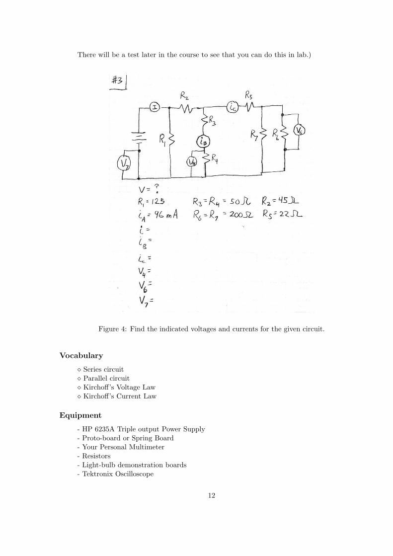
There will be a test later in the course to see that you can do this in lab.)

Figure 4: Find the indicated voltages and currents for the given circuit.

Vocabulary

⋄ Series circuit⋄ Parallel circuit⋄ Kirchoff’s Voltage Law⋄ Kirchoff’s Current Law

Equipment

- HP 6235A Triple output Power Supply- Proto-board or Spring Board- Your Personal Multimeter- Resistors- Light-bulb demonstration boards- Tektronix Oscilloscope

12

- Function generator

Laboratory Time

Four hours

13

Figure 5: Light-bulb demonstration board: Every symbol in this schematic corresponds toa component on the circuit board.

14

2 Internal Impedance and Error Analysis (n=1)

Sources of error generally fall into two classes, systematic errors and random errors. Randomerrors are due to uncontrollable “noise” or reading accuracy of instruments.

Systematic errors are often due to uncalibrated instruments or innaccuracies introduced byfactors such as internal impedance of the measuring device.

Therefore, an important property to know about a voltmeter (or an oscilloscope) and a powersupply (or a battery) is its internal impedance.

Measurements

1. Calibrate a Fluke multimeter (not your meter) vs. a resistance standard and a voltagestandard. (Calibration involves plotting Vmeas = G × Vstd + B). In a simple calibrationthere is both a “gain (G) ” and an “offset” (B) error. Take a half a dozen voltage andresistance data points using the full range of the resistance and voltage standards. I onlyhave a single voltage standard, so you will have to share. If you find yourself waiting around,you can proceed to step 3 and borrow the standards later.

Assume that the standards are perfectly correct. After you have calibrated your meter, useit to measure the voltage of one of the standard cells around the room. How close does yourresult come to the number on the standard cell?

Record GV , BV , BR, and GR in your notebook. You will use them to correct your mea-surements in the rest of the lab. However, there will still be measurement errors.

2. If your voltmeter read 1.000 V, what is your best estimate of what the voltage really is?Also, what do you think is the absolute error on this measurement. What if your meterread 10.00 V? What about 10 mV? What is your best estimate on the error in resistance ifyour meter reads 0 Ω? 10 Ω? 1 kΩ? 1 MΩ?

3. Take measurements and do calculations to find the internal impedance of a Fluke 7X multi-meter when it is set to measure voltage. Use the circuit shown below in figures “a” and “b”,with at least three values for the resistance R. Use (at least) the following values: R=22MΩ, 1.5 MΩ, and 150 kΩ.(NOTE: You have a choice about what voltage to set your power supply to to do this ex-periment. Does it matter? Set it to whatever voltage is likely to give you the most preciseresult. Please note: Do NOT use the voltage standard as your power supply.)

4. Find the internal impedance of an oscilloscope at the BNC connector on the chassis of theoscilloscope.

5. Draw a circuit diagram of a circuit to measure the internal impedance of a small battery.(Indicate the battery itself as an “ideal battery” in series with an internal impedance).

6. Make measurements to find the internal impedance of a 9-V battery.

7. The experiment you just did is probably somewhat destructive to the battery. So let’s finishthe job. Choose a 1/4 Watt resistor of such a value that when you connect it to a batteryyou will exceed its power rating by a factor of about twenty. Note you must take the internalimpedance of the battery just measured into account in doing this calculation or you willpick to large a resistor. Connect your 9-V battery and get your hands away quickly. Whathappens?

15

V δV ∂Ri

∂V∂Ri

∂V δV R δR ∂Ri

∂R∂Ri

∂R δR VB δVB . . . δRi

Table 2: Table listing each value of resistance and each voltage, the uncertainties in each, andthe partial derivatives of the internal impedance with respect to the resistances measured. Theseare the quantites required by the general error analysis formula of Taylor. NOTE: In order tofind the partial derivatives, you need to derive an explicit expression for Ri in terms of R, VB andV . This derivation should be in your lab report, as should the expressions for partial derivativesthemselves.

8. If you enjoyed this destruction, you can take it up a notch. Find an aluminum plate andplace it on your lab bench because you are going to produce something red-hot and we donot want scorch marks. Working over the plate, wrap a single strand of steel wool aroundyour battery terminals. It will glow red hot and melt almost instantly. You have made afuse!

Calculations and Analysis

9. Calculate uncertainties in the internal impedance of the voltmeter (not the oscilloscope) foreach value of resistance used. Use the general formula for propagation of errors given inthe introduction to this lab manual. Make a table like Table 1. (See the formula in theintroduction to this manual) What is your best estimate for value of the internal impedance?

Vocabulary

⋄ Random Error⋄ Systematic Error⋄ Input impedance⋄ Output impedance⋄ Equivalent circuit⋄ Open-circuit voltage⋄ Short-circuit current

Equipment

- Voltage Standard- Resistance Standard- Oscilloscope—one only- Fluke 7X multimeter—one only- Resistors- Power supply- 9V Battery and battery clip

Laboratory Time

Two hours

16

Figure 1: Circuits for measuring the internal impedance of a voltmeter. (a) Circuit to find VB.(b) Circuit to find Ri after VB is known.

References

Taylor, J. R., An Introduction to Error Analysis, University Science Books, Sausalito, California,1997.

17

3 Complex Impedance (n=1)

Since complex numbers are widely used in physics and electrical engineering, it is useful to seehow a complex number can be measured. Here is an experiment to do that.

The experiment

The impedance of a capacitor and resistor in series is a complex number. Determine the compleximpedance of a resistor (R) and capacitor (C) in series by applying a sinusoidal voltage acrossthe series combination and then doing the following:

1. Sketch the circuit you intend to build. It consists of capacitor C connected to the centerpin of the function generator output, followed in series by resistor R. [Note: The style ofconnector used on our function generator and oscilloscopes is called a “BNC” connector].

2. Build the circuit and probe the total voltage from the function generator VFG on one ’scopechannel.

3. Measure the current I through the circuit by probing the voltage across resistor R.

4. Measure the relative amplitude and phase of VFG and I for an input frequencyf = 200 Hz.Hint: Get both signals on the oscilloscope at once. Trigger on the input voltage and setthe trigger level to 0V. This is a way to easily quantify the phase shift between the appliedvoltage and current.

5. Copy the two waveforms into your lab book and label them VFG and VR. The graph shouldbe accurate enough to see the relative phases and amplitudes of the waveforms. You will bereferring to this graph in future labs.

6. Based on your measurements and the theory outlined on the next page, calculate the compleximpedance Ztotal of the circuit as well as the impedance ZC of the capacitor by itself. Assumethat your measurement of the resistor is correct. (You did measure the resistor, didn’t you?).Finally, calculate the capacitance of the capacitor.

7. Repeat all of the above for f = 1000 Hz (You may omit the sketch. You will not it will bedifficult to do).

8. Make an independent measurement of the capacitance (your multimeter will do it). Usingthe measured values ofR and C, work backwards to predict what phase shifts and amplitudesyou would have expected to see. Comment on the agreement (or lack thereof).

Equipment

- Oscilloscope- Function generator- Capacitance meter- Ohmmeter- R=33 kΩ Resistor- C=0.047µF Capacitor

18

Laboratory Time

Two hours

About Complex Impedance

Complex impedance (generally denoted by the symbol Z) is a useful concept because it allowsinductors (L) and capacitors (C) to be treated by the same rules as ordinary resistors (R). (Note:These rules were discussed in the lab called “Circuits”.) The complex impedance of a capacitoris ZC = 1

iωC , where ω is the angular frequency of the applied sine wave. Complex impedanceZ is expressed in units of Ohms just like ordinary resistance R. Likewise, the normal rules forcombining resistors in series and parallel can be used for complex impedances.

Recall that for a voltage divider made of ordinary resistors R1 and R2 in series:

VOUT

VIN= R2/(R1 +R2) (7)

(This formula assumes that VOUT refers to the voltage drop across resistor R2) A complexvoltage divider can be made of any combination of passive components with complex impedanceZ1 and Z2 in series leading to:

VOUT

VIN= Z2/(Z1 + Z2) (8)

Derivation of Complex Impedance of a Capacitor and an Inductor

First, let’s generalize Ohm’s Law from V = IR to V = IZ. Next, apply a sinusoidal voltage tothe circuit under study:

V (t) = V0 cos(ωt+ φ) = Re[

V0ei(ωt+φ)

]

. (9)

Current is in general defined I = dQ/dt. For a capacitor Q = CV , so I = C dV/dt. Usingthe form of V(t) above, we obtain I = C iωV (t). Solving for V(t) we get V (t) = I

iωC . Thus weidentify 1

iωC as the complex impedance of a capacitor (ZC).Given the equation V = LdI/dt for an inductor, see if you can apply a similar argument to

derive the complex impedance for an inductor (ZL).

Going from measured quantities to impedances

In your experiment, you are measuring VFG(t) and I(t). For simplicity, assume that VFG(t) =ℜ(eiωt), with φ = 0. Then Ohm’s law becomes V0e

iωt = I0ei(ωt−φ) Z0e

iφ. Inspection should showyou that you can calculate Z0 from your V0 and I0 measurements. Further, when you measure−φ in the current in steps 3–5 of the experiment, you are really measuring φ in the impedance.

Refresher on Complex Arithmetic

Recall that for any complex number Z:

Z = x+ iy = Z0eiφ (10)

where Z0 =√

x2 + y2 and φ = atan(y/x). Also Z20 = Z∗ Z, where Z∗ ≡ x− iy. Finally, it is

useful to know that if Z = 1a+ib , then Z∗ = 1

a−ib

19

4 Magnetic Field, Inductance, Mutual Inductance, andResonance (n=2)

Introduction

In this laboratory exercise you will learn

• how to determine impedance from measurements of an alternating current and voltage,

• how to calculate mutual and self inductance,

• how to measure the amplitude of an oscillating magnetic field,

• how a circuit behaves around a resonance, and

• how a transformer works.

This is a good time to review the concepts listed above in a junior-level textbook on electricityand magnetism.

Laboratory Work

Figure 1: Circuit for measuring impedance and self-inductance and exploring what happensaround a resonance.

1. Hook up the circuit in the figure below. According to the manufacturer, the coil (called“Outer Coil”) has 2920 turns of 29 AWG wire (wire diameter φ = 0.29 mm). The resistanceR = 220Ω will be used to measure the current in the circuit.

2. Self inductance:

(a) For a frequency f = 1000 Hz, measure the amplitudes of the voltage VFG(t) from thefunction generator and the voltage VR across the resistor. Also measure the phasedifference between VFG and VR. Make sketches of the waveforms and label VFG andVR. Compare these sketches to those you made in the lab called “Complex Impedance”.Note how they differ. Estimate uncertainties of the amplitudes and phase.

(b) From the measurements construct the complex functions V (t) and I1(t).

(c) Find the total impedance ZT ≡ V (t)/I1(t), which will be a complex number.

20

(d) Subtract the impedance of the resistor ZR ≡ R + 0i from the total impedance ZT tofind the impedance of the Outer Coil, Z1.

(e) The impedance of the Outer Coil is Z1 = R1 + iωL1, where R1 is the resistance of theOuter Coil due to the resistance of the wire. L1 is the self inductance and ω is theangular frequency (radians/second). R1 can be measured with an ohmmeter, whichdoes not see the inductance because it applies a steady (DC) voltage. Compare yourtwo values of R1 with the value given by the manufacturer.

(f) Calculate the self inductance of the Outer Coil L1 and estimate its uncertainty. Com-pare L1 with the value given by the manufacturer, which is 63 mH (after correctingthe typo in the manufacturer’s instruction sheet).

3. Resonance:

(a) Look for a resonance betwee 35 and 40 kHz. It will show up clearly as a null in yourmeasurement of current. Measure this frequency to three significant figures.

At the resonant frequency the Outer Coil has a significant capacitance in addition toinductance. The capacitance arises from the dielectric gap between adjacent turns ofthe wire. (The dielectric is partly air and partly the enamel coating on the wire.)A model for the coil is a perfect inductance L1 with capacitance C1 in parallel. Atsome frequencies, the parallel combination acts more like an inductor, and at otherfrequencies, the parallel combination acts more like a capacitor; you can understandthis better by calculating the impedance of the parallel combination from the individualimpedances of an inductor and capacitor.

Compare the relative phases of VFG(t) and I1(t) at frequencies above and below theresonant frequency. Sweep back and forth through the resonance and note what youobserve about the phase. This is not a precision measurement. You are merely tryingto observe what happens to the phase as the circuit passes through resonance.

(b) Disconnect the oscilloscope probe that measures V (t) and use it to measure the voltageV2(t) across the Search Coil, which is wound on a 3/4 inch diameter wooden dowel.Keep the other probe connected across the resistor R so you can watch the behavior ofthe current. Place the Search Coil inside the Outer Coil and observe what happens toV2(t) and I1(t) as the frequency is increased through the resonant frequency. Noticethat while I1(t) is nearly zero at resonance, V2(t) is not. But V2(t) is proportional todB/dt which is proportional to the rate of change of current in the Outer Coil. Howcan this happen when I1(t) is nearly zero?

4. Magnetic Field Amplitude and Mutual Inductance.

The Search Coil can be used to find the magnetic field produced by the Outer Coil. Forthe calculations of magnetic field amplitude and mutual inductance described below, setthe function generator for a large amplitude and a frequency f = 1000 Hz and make thefollowing measurements:

(a) Voltage across the resistor in series with the Outer Coil ( for determining the current).

(b) Voltage and phase across the leads from the Search Coil.

5. Transformer.

21

Figure 2: Circuit with Outer Coil and inner Search Coil. The Search Coil can be used to find themagnetic field from the Outer Coil. There is a mutual inductance between the two coils. As aunit, the two coils are a transformer.

The two coils together are a transformer. In a transformer, power flows from the primarywinding (Outer Coil in this case) to the secondary winding (Search Coil in this case). Removethe resistor from the primary circuit so that the function generator is connected directlyto the primary winding (Outer Coil). And then, for calculations described below, do thefollowing:

(a) Find and note the range of frequencies for which V2/V1 is nearly constant. Set thefrequency somewhere in the middle of this range before making the following twomeasurements.

(b) Measure the voltage V1 across the primary winding (Outer Coil).

(c) Measure the voltage V2 across the secondary winding (Search Coil).

Calculations and analysis

6. Derive an approximate expression for the magnetic field strength B near the center of theOuter Coil when the current through that coil is I1, the number of turns of wire is N1,and the length of the coil is ℓ1. Make the approximation that B = 0 outside the coil. Thequantities I1, N1, and ℓ1 have subscript 1 to indicate that they are associated with theOuter Coil (also called the primary of the transformer). Later, the subscript 2 will be usedfor variables associated with the secondary coil of the transformer (Search Coil).

7. Derive an approximate expression for the self-inductance of the coil. Your expression willinvolve N1, A1, ℓ1 and physical constants. A1 is the area enclosed by one turn of wire inthe coil.

8. Use the results in the previous items to estimate a numerical value for the inductance of thecoil. Also estimate its impedance Z1 = iωL1 at a frequency f = 1 kHz.

9. Compare the inductance L1 of the Outer Coil deduced from your measurements of voltageamplitude and phase with the value obtained from the equation for L1 above. Can thediscrepancy be explained by the uncertainty in the measured values? If not, can you comeup with a systematic reason for the error, and can you perhaps come up with a way tocalculate L1 more accurately? Explain, and do it.

22

10. Starting with one of Maxwell’s equations, develop the equations for determining B fromthe voltage induced in the Search Coil, given the cross-sectional area A2 and number ofturns N2 of the Search Coil. Variables associated with the Search Coil will have subscript 2.Compare the B value derived from your measurements with that calculated as in (1) above,using the actual value of the current.

11. The combination of the Outer Coil and Search Coil constitutes a mutual inductor. Derivethe following approximate equation for the mutual inductance between the Outer Coil andthe Search Coil using the approximate expression for B above:

M12 = µ0N1N2A2/ℓ1. (11)

In addition, compute the induced voltage in the Search Coil.

12. Derive the following expression for the ratio of voltages of a transformer:

V2

V1=

N2A2

N1A1, (12)

Compare your measured value with that predicted from the above expression.

13. Notice that the above equation predicts that V2/V1 will be independent of frequency. Forwhat range of frequencies is this true? For extra credit, you may speculate on why theequation fails, or at low frequencies.

14. Using the value for L1 and the resonant frequency, calculate the capacitance of the coil.

Vocabulary

⋄ Search coil⋄ Mutual inductance⋄ Tank circuit⋄ Primary winding⋄ Secondary winding

Equipment

- Outer Coil (2920 turns)- Search Coil (50 turns wound on wood)- Oscilloscope- Function generator- 220 Ω resistor

Laboratory Time

Four hours

23

5 Hysteresis (n=2)

Introduction

A system is said to exhibit hysteresis when the state of the system does not reversibly followchanges in an external parameter. In other words, the state of system depends on the historyof the system (“history-sis”). The classic examples of hysteresis use Ferromagnetic materials.The state of the system is given by the magnetic moment per unit volume, M, and the externalparameter is the magnetic field, H. In this experiment, we explore hysteresis in the ferromagneticcore of a transformer by measuring both the magnetic flux density B and the magnetic intensityH in the core. The variable M can be deduced from H and B.

The magnetic intensity vector H is defined by the equation

H ≡1

µ0B−M , (13)

where B is the magnetic flux density (or magnetic induction), µ0 is the magnetic permeabil-ity of free space and M is the macroscopic magnetization. The macroscopic and microscopicmagnetizations are related by the defining equation

M = lim∆V→0

1

∆V

∑

i

mi . (14)

M is the vector sum of the atomic magnetic moments divided by the volume, ∆V , of the sample.For an isotropic, linear material, M is linear in H, as

M = χmH , (15)

where the dimensionless magnetic susceptibility χm is assumed constant. In this case equation (13)becomes,

H =1

µ0B−M (16)

so that µ0H = B− µ0χmH (17)

and B = µ0(1 + χm)H . (18)

By comparing this last equation with the free space equation,

B = µ0H , (19)

the magnetic permeability, µ, of the material is defined to be

µ = µ0(1 + χm) . (20)

24

The relative permeability Km is defined as

Km =µ

µ0(21)

so that Km = 1 + χm . (22)

In a ferromagnetic material, the magnetization is produced by cooperative action betweendomains of collectively oriented atoms. Ferromagnetic materials are not linear, so that

χm = χm(H) . (23)

However, the above equations are still applicable if we realize that µ is no longer a constant, thatis

µ(H) = µ0[1 + χm(H)] (24)

andB = µ(H)H . (25)

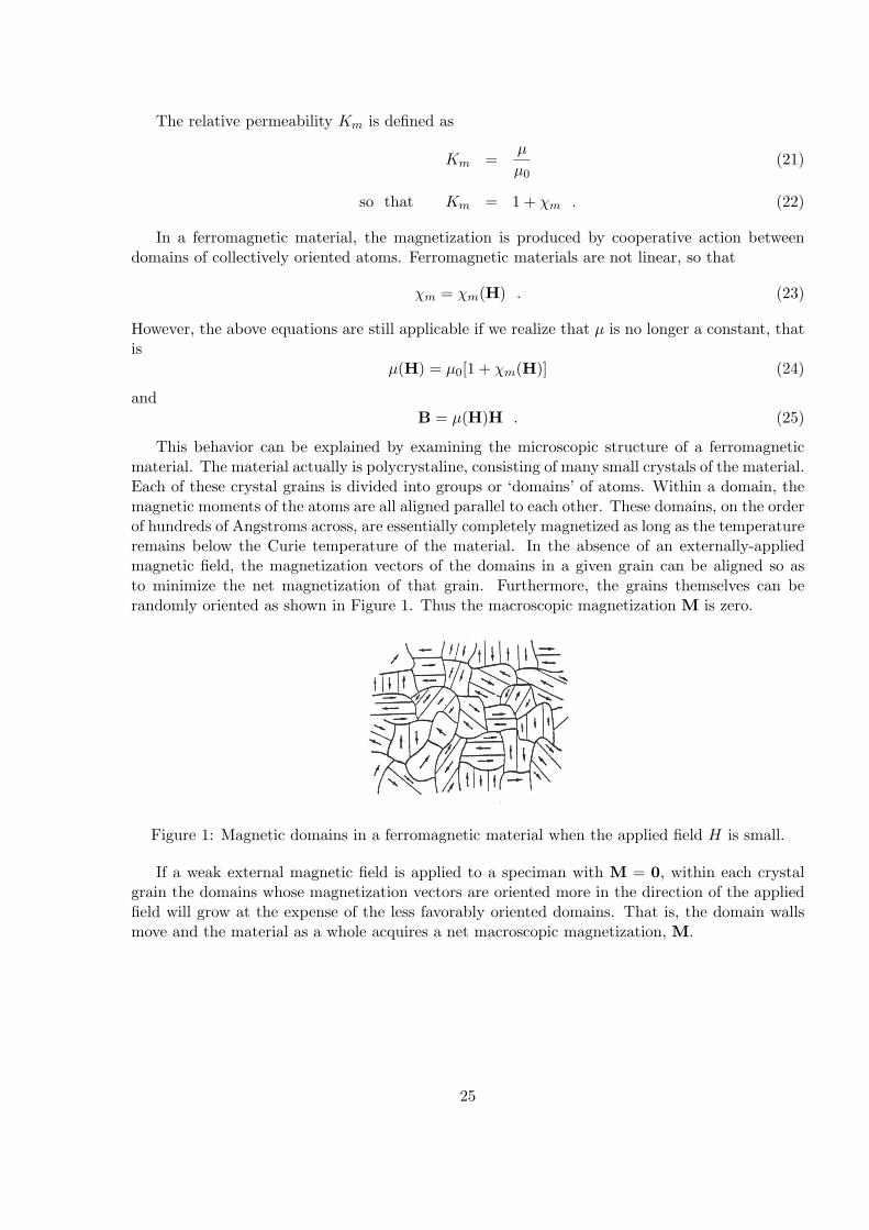
This behavior can be explained by examining the microscopic structure of a ferromagneticmaterial. The material actually is polycrystaline, consisting of many small crystals of the material.Each of these crystal grains is divided into groups or ‘domains’ of atoms. Within a domain, themagnetic moments of the atoms are all aligned parallel to each other. These domains, on the orderof hundreds of Angstroms across, are essentially completely magnetized as long as the temperatureremains below the Curie temperature of the material. In the absence of an externally-appliedmagnetic field, the magnetization vectors of the domains in a given grain can be aligned so asto minimize the net magnetization of that grain. Furthermore, the grains themselves can berandomly oriented as shown in Figure 1. Thus the macroscopic magnetization M is zero.

Figure 1: Magnetic domains in a ferromagnetic material when the applied field H is small.

If a weak external magnetic field is applied to a speciman with M = 0, within each crystalgrain the domains whose magnetization vectors are oriented more in the direction of the appliedfield will grow at the expense of the less favorably oriented domains. That is, the domain wallsmove and the material as a whole acquires a net macroscopic magnetization, M.

25

For weak applied fields, movement of the domain walls is reversible and χm is constant. Thusthe macroscopic magnetization M is proportional to the applied field,

M = χmH , (26)

andB = µH , (27)

where µ is constant.For larger fields the domain wall motion is impeded by impurities and imperfections in the

crystal grains. The result is that the domain walls do not move smoothly as the applied field issteadily increased, but rather in jerks as they snap past these impediments to their motion. Thisprocess dissipates energy because small eddy currents are set in motion by the sudden changes inthe magnetic field and the magnetization is therefore irreversible.

For a sufficiently large applied field the favorably oriented domains dominate the grains. As theapplied field is further increased, the magnetization directions of the less well oriented domains areforced to become aligned with the applied field. This process proceeds smoothly and irreversiblyuntil all domains are aligned with H. Beyond this point, no further magnetization will occur.The magnitude of M = |M| at this point is called the “saturation magnetization.” A graph ofB = |B| versus H = |H| for the above process is shown in Figure 2. This graph, which starts atB = 0 and H = 0, is called the normal magnetization curve.

Figure 2: The normal magnetization curve of B versus H.

For large H, the domains appear as in Figure 3.

Figure 3: Ferromagnetic domains when the applied H is large.

The alteration of the domains and their direction of magnetization gives rise to a permanentmagnetization which persists even after the applied field is removed.

26

Figure 4: Magnetic hysteresis loop.

If we try to demagnetize the material by decreasing H, the B vs. H curve of Figure 2 is notfollowed. Instead, B does not decrease as rapidly as does H. Thus, when H decreases to zero,there is still a non-zero Br, known as the “remnance.” Only when H reaches the value −Hc doesB become zero. This value Hc is called the “coercive force.” Continuing the cycle H1, zero, −H1,zero, and back to H1, the B–H curve looks like that in Figure 4. Since B always “lags” behindH, the curve in the above graph is called a “hysteresis” loop (from the Greek “to lag”).

The area inside the loop can be shown to be proportional to the energy per unit volume thatis required to change the orientation of the domains over a complete cycle (Warburg’s Law):

W =

∫

vol

∮

cycleHdB dτ . (28)

This energy goes into heating the specimen, and is in joules if H, B and v are measured in A/m,Tesla and m3, respectively.

Applying Maxwell’s Equations

Using the apparatus diagrammed in Figure 5, we can observe the hysteresis curve of a ferromag-netic material by the following technique. Suppose we wind two coils of wire on a torus of thematerial. Since ferromagnetic materials are good “conductors” of magnetic flux, the couplingconstant between the two coils will be close to one.

Since both the magnetizing field H and the voltage drop across R1 are proportional to theinstantaneous magnetizing current, the horizontal deflection on the scope is proportional to H.

Faraday’s Law (one of Maxwell’s equations),

∇×E = −∂B

∂t, (29)

is what we need to calculate the voltage Vs across the secondary winding:

Vs = N2AdB

dt. (30)

Integrating gives

B =1

N2A

∫

Vs dt . (31)

27

Figure 5: Schematic of apparatus to generate and display hysteresis loops.

R2 and C across the secondary act as an integrator. If the resistance R2 ≫1ωC , then the current

in the secondary is determined almost entirely by R2, so that we may write is = Vs/R2. In thecapacitor, the current is clearly dq

dt , so

dq

dt= is =

Vs

R2. (32)

Hence the potential difference across C at any instant is

Vy =q

C=

1

R2C

∫

Vs dt =N2AB

R2C, (33)

so that the vertical deflection is proportional to B:

B = kBVy . (34)

An analysis of the transformer primary circuit begins with Ampere’s Law, another one ofMaxwell’s equations,

∇×H = J+∂D

∂t, (35)

and yieldsH = kHVx (36)

for the average of H around the iron core. after recognizing that the displacement current can beneglected at low frequencies.

Laboratory Measurements

1. Set up the apparatus using a 10Ω, 5W resistor for R1, a 500kΩ resistor for R2, and a 0.1µFcapacitor for C. To display a hysteresis loop, run the oscilloscope in xy mode and displayVx on the x axis and Vy on the y axis. Be sure to include the isolation transformer (why?).

2. Starting with the Variac at zero, slowly turn up the voltage in increments such that eachsuccessive increment produces a hysteresis curve that is distinguishable from the previousone. Trace these curves, continuing until the material reaches saturation.

3. For the Variac setting that gives the largest hysteresis curve, measure the temperature risein a one-minute time interval.

28

Calculations and Analysis

4. Transformer Primary: Starting with the Maxwell equation that relates the curl of ~Hto ~J , derive (36) and find an expression for kH . Draw a figure showing the path for the lineintegral and the area for the surface integral.

5. Transformer Secondary: Starting with the Maxwell equation that relates the curl of~E to the time derivative of ~B, derive (30), (31), (33), and (34). Draw a large, clear figurethat shows the path for the line integral and the area for the surface integral superimposedon the transformer.

6. Choose one of your largest hysteresis loops and, using Warburg’s law, calculate the energyloss per cycle due to hysteresis, the temperature rise of the core per cycle and the numberof cycles and elapsed time necessary to raise the temperature of the core by 1C. Be carefuldoing this calculation; it will take time; be sure your result is reasonable.

7. Plot the normal magnetization curve using the end points of the hysteresis loops.

8. From the normal magnetization curve (B vs. H), plot the relative permeability µ/µ0 of thematerial as a function of H.

9. What is the theoretical limiting slope of the magnetization curve B(H) when H → ∞?(Hint: start with the most fundamental relation between H and B: B = µ0(H+M).) Esti-mate the error in your measured value. Compare the theoretical value with your measuredvalue and explain why they differ.

10. To see that hysteresis is a common phenomenon and a simple idea, do the following. Push ablock of wood in a straight line on a table top, and then push it back to its original location.Make a hysteresis plot for this cycle, and show which lines on the plot correspond to whichmotions of the block of wood on the table. The axes for the plot should be position andforce, so that the area enclosed by the hysteresis loop is the mechanical energy transferredto heat in the cycle. NOTE: You do not need to measure any forces. Push the block withyour finger with slowly increasing force. Move it a bit, then push it back. Note qualitativelywhat happens. Use this to make your plot. You can put numbers on your axes, but theywill of course be very approximate.

Vocabulary

⋄ Hysteresis Loop⋄ Soft magnetic material⋄ Saturation Magnetization⋄ Remanence

Reference

D. J. Griffiths, Introduction to Electrodynamics, Prentice Hall, Englewood Cliffs, New Jersey,1989.

R. G. Lerner and G. L. Trigg, Encyclopedia of Physics, Second Edition, VCH Publishers, Inc.,New York, 1991, pages 529–530.

29

Equipment list

- Isolation transformer- Variac- AC patch cord- Ferromagnetic Torus (Rowland Ring)- Oscilloscope- Resistor R1 (10 Ω, 5 W) and Resistor R2 (470–530 kΩ)- Capacitor C (0.1 µF)- Plastic film & fine-tip “sharpie” marker for tracing oscilloscope pattern- Thermometer and insulation

Laboratory Time

Four hours

30

6 Diodes and Transistors (n=1)

Diodes and transistors are two of the fundamental building blocks for modern digital electronics.The exercises below are a step toward understanding their properties.

Some aspects of the behavior of a transistor can be understood from the following two prin-ciples:

1. Current starts to flow in the forward direction (the direction of the arrow in circuit symbols)through diode junctions when the voltage across the junction reaches a threshold, which isabout 0.6 volts for silicon diodes. The base-emitter and collector-base junctions of transistorsare diodes.

2. Transistors amplify currents. The current that flows from the collector terminal to theemitter terminal is called Ic. The current that flows from the base terminal to the emitterterminal is called Ib. The current gain is

hFE =IcIb

. (37)

Diode Characteristics

The diode we will use is the emitter-base junction of a NPN transistor. The flat side of thetransistor has labels for the three pins: e, b, c, for emitter, base, collector.

1. Using the circuit of Figure 1 measure the voltage Vbe across the diode and deduce the currentIb through it. Measure enough values to make a good graph of Ib(Vbe).

2. Then reverse the polarity of the voltage applied to the series combination and repeat themeasurements. Let both Vbe and Ib be negative numbers after reversing the polarity.

3. Combine the data from both polarities on a single graph of Ib(Vbe). This function, Ib(Vbe),is called the constitutive relation for the diode.

4. Make a few measurements at large voltages using the collector/base junction instead of theemitter/base junction of the transistor. Comment on the difference between the two diodes.

5. Use the circuit of Figure 2 to rectify an AC signal. Sketch V1(t) and VR(t) from the oscil-loscope; use the same voltage scales and the same zero position for both V1(t) and VR(t).Explain what you see using the constitutive relation for the diode and the constitutiverelation for a resistor (Ohm’s law).

Transistor Amplifier

In the circuit of Figure 3, a sine wave V1(t) from a function generator drives a current Ib throughthe base-emitter junction of a transistor; the resistor in series with the junction limits the current.The purpose of the following measurements is to study amplification by the transistor.

6. Use the two inputs of the oscilloscope to compare Vce(t) and V1(t). Sketch the waveforms.Explain the shape of Vce(t).

7. Call τ the time when Vce is a minimum, which is also when the current Ic is a maximum.For the specific time τ do the following:

31

Figure 1: Circuit for finding I vs. V for a diode.

Figure 2: Circuit to rectify a voltage.

(a) Measure the base current Ib(τ) and the collector current Ic(τ) and calculate the ratioIc/Ib. This ratio is the current gain of the transistor, which is often called hFE inmanufacturer’s data sheets. Compare the current gain you deduce from your measure-ments with the current gain you expect from the manufacturer’s specifications for thetransistor.

(b) Find the power delivered to the base-emitter junction and the power dissipated by theresistor RL, which is called the load resistor. How do you account for the fact that theenergies are different? Where does the extra energy come from?

Vocabulary

⋄ Forward bias⋄ Reverse bias or back bias⋄ Diode drop⋄ Breakdown voltage⋄ Carrier

32

Figure 3: Circuit for studying transistor amplification.

Equipment list

- Power Supply- Function generator- NPN Transistor: 2N4401 or MPSW01- Oscilloscope- Resistors

Laboratory Time

Two hours

33

7 Operational Amplifiers (n=2)

Uses of Operational Amplifiers

Measurements in every branch of science and engineering typically begin with a transducer thatchanges whatever parameter is being measured into an electrical signal for further amplificationand processing. Because of their versatility, superb performance, ease of use, and low cost,operational amplifiers (op amps) have become the main building block for amplification andprocessing of electrical signals before they are digitized and ingested by a computer. Operationalamplifiers are used in circuits to perform the following functions:

• Amplifying.

• Adding, subtracting, and multiplying.

• Integrating and differentiating.

• Detecting peaks and holding them.

• Filtering (low pass, high pass, and band pass).

• Modulating and demodulating.

Books listed under References below show many useful circuits using operational amplifiersand explain how they work in more detail than we give in the next section.

What Operational Amplifiers Do

As you would expect, an amplifier in general increases some electrical quantity, usually voltage. Ingeneral, VOutput = A×VInput where the factor A is called the Gain of the amplifier. An integratedcircuit operational amplifier such as we will be studying in this lab amplifies the voltage differencev+ − v− between its ‘+’ and ‘−’ inputs (see Figure 1). The output voltage is

V2 = AOL(v+ − v−) , (38)

where AOL is the open-loop voltage gain of the amplifier.Two properties of operational amplifiers make them particularly useful:

• The open-loop gain AOL is large (typically 105 at low frequencies).

• The resistance Rin between the + and − inputs is large (typically 10 MΩ for operationalamplifiers which use bipolar junction transistors (BJT) amplifiers, and 1010Ω or higher foroperational amplifiers which use field effect transistors (FET’s).

Operational amplifiers are used by providing negative feedback (usually resistance) from theoutput to the − input, which substantially reduces their gain from its open-loop value. Thisnew gain is called the closed-loop gain and we will denote it as G. When the open-loop gainAOL is much greater than R2/R1 (see Figure 1), then the voltages v+ and v− are very nearlyequal. Furthermore, when the resistance used in the feedback loop is small compared with theinternal resistance of the operational amplifier, then the currents into the + and − inputs can beneglected. When these conditions are true the operational amplifier is said to be ideal. An idealoperational amplifier can be analyzed by adding the following two simple rules to the usual rulesfor circuit analysis:

34

1. The + and − inputs are at the same potential.

2. No current flows into either input.

For an ideal operational amplifier, the closed loop gain G depends only on the feedback elementsand not on its open-loop gain AOL nor on its internal resistance.

Figure 1: Inverting and non-inverting configurations.

The Experiment

Here is a hypothesis for your consideration:

OP-AMP GAIN HYPOTHESIS: “The closed-loop gain of an inverting amplifier isG = −R2/R1 and the gain of an non-inverting amplifier is G = R2/R1.”

The circuits for inverting and non-inverting amplifiers are shown in Figure 1.The above hypothesis is only even approximately true for a so-called ideal amplifier for which

the output is simply a costant multiple of the input at all amplitudes and frequencies. However,there is so such thing as an ideal amplifier. In the first three tests, you will learn the limitations ofop-amps by observing clipping, slew-rate limit, and band-width limit. In the fourth test, you willquantitatively test the OP-AMP GAIN HYPOTHESIS for DC voltages where op-amps behavealmost ideally. Your write-up should have an entry corresponding to each of the numberedmeasurements or calculations below.

Build an inverting amplifier. Use R1 ∼ 10 kΩ and R2 ∼ 100 kΩ.NOTE: Up until now, your circuits have been “passive”, which means there is no need topower them. Op-amps are “active”, they need power, as well as inputs and outputs. Wewill call the power voltages VPS (PS for power-supply). We will call the input and outputvoltages (also called “signal voltages”) V1 and V2. Perhaps this discussion will reduce yourconfusion about “what wire goes where“

35

Test the basic operation. Use a function generator to supply voltage V1 and look at V2 with anoscilloscope. Set the frequency to about 100 Hz and try out the various available functions—square wave, triangle wave, and sine wave just to make sure the op-amp is basically working.V2 should look just like V1 but be roughly ten times as large.

Study non-ideal effects

1. To observe clipping set your power supply voltage (VPS) to VPS = ±10 V . Then set V1 to1.5 Vpp. Leave the frequency at 100 Hz and draw the output waveform for inputs that aretriangle, square, and sine-wave.

2. Now repeat the observations and sketches except with VPS = ±12 V and finally VPS =±18 V .

3. Why do you think this effect is called clipping?

4. Now we will study slew-rate limit and band-width limit. Slew-rate limit is more noticeablefor large V1. Band-width can only be measured for small V1 (perhaps V1 = 5 mVpp). Lookup and record in your report the slew-rate and the gain-bandwidth-product (GBWP) onthe op-amp data-sheet.

5. Use a function generator to supply varying AC voltages V1 and increase the frequency untilthe waveform output begins to noticeably differ from the input waveform. Record thisfrequency in the table and sketch the output to indicate how it differs from the input.Below is a table to help you organize your measurements.

6. Op-amps have a finite ”bandwidth”. For sufficiently high frequencies, his means that theamplitude of the output of an op-amp decreases compared to its amplitude at lower frequen-cies. (The bandwidth also depends on the gain of the amplifier.) The bandwidth is alsoreferred to as the “knee”, “3-dB point” or “corner frequency”. All of these terms mean thefrequency at which the output amplitude has fallen to half of the output amplitude at lowfrequencies. Determine the “corner frequency” of your inverting amplifier. (NOTE: Thismeasurement ONLY applies to sine waves at low input voltages (i.e. where slew-rate doesnot affect the results).)

Test Gain Hypothesis

7. Test the OP-AMP GAIN HYPOTHESIS by experiment. Supply about a dozen input volt-ages V1 into your inverting amplifier over a range that will drive its output from near 0.0 Vto saturation (or clipping). Make a table of V1, V2 and Gexpt.

8. Measure each resistance with an uncertainty of less than 0.01 times the value of the resis-tance. Measure V1 and V2, with an uncertainty of less than 0.01 times value of the voltageusing a voltmeter. Plot V2 vs. V1. Using standard methods for propagating errors, estimatethe uncertainty in V2/V1 and R2/R1. Compare the ratio of resistances (Gtheory) with theratio of voltages (Gexpt) from the previous question.

9. Discuss how well the OP-AMP GAIN HYPOTHESIS holds for the inverting amplifier.

36

V1 Input Freq. at which Sketch(mVpp) Wave Output looks of

Shape different from input output

5 Square

50 Square

500 Square

5 Sine

50 Sine

500 Sine

5 Triangle

50 Triangle

500 Triangle

Table 3: If your function generator cannot make V1 as small as 5 mV, build a 10:1 voltage dividerallow this

10. Now modify your circuit to make a non-inverting amplifier and repeat the measurments, thetable, the plot, and the discussion of how well the OP-AMP GAIN HYPOTHESIS holds forthe non-inverting amplifier.

11. Derive equations for the gains of the inverting and non-inverting circuits using the two rulesfor ideal op amps.

12. Do your experimental results agree with the improved theory you just derived?

Vocabulary

⋄ Open loop gain⋄ Closed loop gain⋄ Bandwidth⋄ Corner frequency or Roll-off frequency⋄ Slew Rate⋄ Clipping

References

Powers, Thomas R., The Integrated Circuit Hobbyist’s Handbook, High-Text Publications, SolanoBeach, California, 1995.

37

Horowitz, Paul, and Hill, Winfield, The Art of Electronics, Cambridge University Press, NewYork City, 1989.

Equipment

- Operational Amplifier (LT1001)- Oscilloscope- ±15 volt power supply- Resistors: 10 k and 100 k- Ohmmeter

Laboratory Time

Four hours

38

8 Automobile Circuits (n=1)

There are many interesting and sophisticated applications of electricity and magnetism inautomobiles. The following explorations introduce a few of them.

Laboratory Activities

1. Measure voltage as a function of current through a headlight filament. Plot V (I). Does thefilament obey Ohm’s Law? Explain.

2. Study a headlight. Draw a circuit diagram for it.

3. Operate the ignition circuit. (“Ignition” refers to the process of igniting the air-gas mixturesin the cylinders.) Study it. Draw a circuit diagram for it. Write a short essay on how itworks. Include an explanation of how high voltages are produced.

4. Make a blinking tail light circuit.

After the Lab

5. Compare the energy/volume ratio of a battery with that of a 1 µF laboratory capacitor.

6. Draw a circuit diagram for an automobile’s starter motor. Include the battery, key switch,solenoid relay, and starter motor. Use standard symbols for the circuit elements.

7. Estimate how much current the starter motor draws. Show your calculations.

Equipment List

- 12 V high-current power supply- Headlights- Tail light blinker- Ignition circuit assembly

Laboratory Time

Two hours

39

9 Index of Refraction of Air (n=1)

Even though the wavelength of light in air is only slightly smaller than the wavelength of lightin a vacuum, it can be measured.

Measurements

1. Use the equipment listed below to determine the index of refraction of air.

2. Extrapolate your results to predict the index of refraction at 1 atmosphere (1013.25 mil-libars) and 0o C.

3. What measurement uncertainty leads to the largest uncertainty in the index of refraction?What is the resulting uncertainty in the index of refraction?

Calculations

4. From your data and the ideal gas law, find out how the ratio of pressure to absolute tem-perature, p/T , depends on the fringe number Nf . The fringe number Nf is defined in thefollowing way: fringe number 1 is the fringe you see at the beginning. As new fringes appearas you decrease (or increase) the pressure, number them 2, 3, 4, etc.

5. From theory derive the function Nf (n) where n is the index of refraction.

6. From the above, find the function p(n) relating pressure and index of refraction. Then finda relation between 1− n and p(1)− p(n). Put in numbers to get 1− n. Then find n.

Equipment list

- Hand vacuum pump- Chamber with flat windows- Pressure sensor- Laser- Michelson Interferometer- Thermometer

Laboratory Time

Two hours

40

10 Electric Field, Capacitance, Dielectric Constant (n=1)

Laboratory Work

Measure the dielectric constant of liquid nitrogen.Some of the effort in this laboratory project will be designing the experiment. You will

need to make calculations to see what kinds of equipment the experiment will require. The firstmeasurements should be done quickly and simply to uncover unsuspected problems.

Report

In addition to describing your laboratory work and the results, consider the subtle effect leadingto the Clausius-Mosotti formula in Problem 4.38, Page 200 of D. J. Griffiths, Introduction toElectrodynamics, Third Edition, Prentice Hall, Upper Saddle, NJ, 1999. Can the Clausius-Mosottiformula explain the descrepancy between your measurement and the accepted value of liquidnitrogen? (You should be able to find the polarizability of one nitrogen molecule from the dielectricconstant of gaseous nitrogen.)

Equipment

- Liquid Nitrogen- Air-variable capacitor- Styrofoam containers- Miscellaneous electronic equipment

Laboratory Time

Two hours

41

11 Negative Resistance (n=1)

Introduction

In linear devices such as ordinary resistors, “resistance” could be defined either as dV/dI or asV/I; in either case the resistance of the device would have the same value. What definitionshould be used for non-linear devices such as diodes, neon lamps, and spark gaps? There is someadvantage in defining resistance for these kinds of devices as dV/dI. Because of this definition,these devices exhibit negative resistance, and because of the negative resistance they can be madeto oscillate in special circuits.

Laboratory Work

1. This experiment will use a high voltage power supply; ask the instructor to look at yourcircuit before turning on the supply.

2. Find the relation between voltage V and current I for a neon lamp. This relation is calledthe “constitutive relation” for the neon lamp.

3. Use the constitutive relation to design and construct an oscillator. A capacitor and a resistorwill be required in the circuit. Draw a diagram of your circuit. Measure the frequency ofthe oscillator. (HINT: The capacitor needs to be put in parallel with the lamp, while theresistor needs to be in series with the combination. Based on your measurementsso far, youshould be able to pick a resistor and capacitor that will work well.)

4. Now that you have seen the oscillator work once, you are more likely to understand what isgoing on. Select a different resistor or capacitor with the goal of either doubling or halvingthe oscillator frequency (you decide which you want to do. If your first frequency came outsmall, you might want to double it, but if the flashing is pretty rapid, you might aim tohalve the frequency.)

Calculations and Analysis

5. From the values of the capacitor and the resistor and the voltage at which the neonlamp becomes conducting, calculate the frequency of the oscillator. Compare your cal-culated frequency with the measured frequency. Repeat the calculation for the secondresistor/capacitor set you choose.

Equipment list

- High voltage supply- Voltmeters- Neon lamp- Assorted parts

Laboratory Time

Two hours

42

12 Superconductivity (n=1)

Introduction

The discovery of ceramic compounds that are superconductors when immersed in liquid nitrogenhas made it possible to investigate some properties of superconductivity using very simple appa-ratus. In this lab we will use a commercial high-temperature-superconductivity experiment kit tostudy some of aspects of superconductors. The kit contains a disk of ceramic superconductor, amodule consisting of a smaller ceramic superconductor disk with an attached thermocouple, andtwo very strong, small magnets.

A superconductor is a substance which acts like a perfect conductor when its temperature isbelow some critical value, the critical temperature Tc. Thus when T < Tc a superconductor actsas if its resistance were zero, so that if a current were to be established in a ring of superconductorit would persist indefinitely.

In 1933, Meissner discovered that a magnet was repulsed by a superconductor, an effect nowknown by his name. The following are some considerations of how the Meissner effect might comeabout.

Suppose that a strong magnet is brought up to a superconductor so that the superconductorexperiences a finite dB/dt. Then an emf would be induced in the superconductor such that acurrent would begin to flow. This induced current would continue to flow after the magnet stopsmoving (dB/dt = 0) because zero voltage will maintain a current when the resistance is zero.According to Lenz’s law the induced current will be in a direction such that the B field due to itwould be opposed to the B field of the magnet. Thus there would be a repulsive force betweenthe small magnet and the superconductor. If the small magnet had a sufficiently strong field thenthe repulsion could result in the magnet being levitated above the superconductor.

However, if the magnet were placed on the superconductor while the superconductor waswarmer than the critical temperature, and then the superconductor was cooled to below the criticaltemperature, the magnet would not be levitated since dB/dt would never have been different fromzero. Nevertheless, if one were then to try to remove the magnet from the superconductor, therewould be an attractive force between the two of them resisting the removal of the magnet due tothe B field of the current induced in the superconductor as the magnet was moved. Since there iszero resistance in the superconductor we might expect that the induced current would be entirelyon the surface and not in the interior of the superconductor.

Another way that a superconductor might repulse a magnet is if microscopic magnetic dipolesare induced in the superconductor which then oppose the applied field. Then, inside the su-perconductor there would be zero B field, and the external field of the dipoles induced in thesuperconductor would repel the source of the applied field, that is, the magnet. The superconduc-tor would then be described as diamagnetic. This implies that the effect would be a volume, orbulk effect, becoming stronger when the volume of the superconductor is increased. In this case,if the magnet were placed on the superconductor before it was cooled, as the superconductor be-came superconducting it would exclude the magnetic field from its interior and the magnet wouldbe levitated. Of course, this assumes that the strength of the magnet is sufficient to support itsown weight.

This experiment is divided into two parts. In the first part you will study the Meissner Effect.In the second part you will determine the critical temperature of the ceramic superconductor.

43

Preparation Before Lab

Read the article on Superconductivity by Philip B. Allen in Encyclopedia of Physics, SecondEdition, edited by Lerner and Trigg, VCH Publishers, New York, 1991, pages 1198–1203.

Safety Procedures

Liquid Nitrogen

Liquid nitrogen (LN2) is COLD, it will kill skin cells by freezing them.

• Wear safety glasses when using LN2.

• Do not allow any LN2 to contact your body.

• Do not touch anything that has been immersed in LN2 before it has warmed to roomtemperature. Use the plastic tweezers provided.

• Be very careful to avoid splashing of the LN2.

• Avoid overfilling any vessel or spilling the LN2.

• Do not put LN2 in any vessel with a tight-fitting lid.

• The extreme cold of LN2 will damage many surfaces, so do not pour LN2 on or in anythingnot intended for LN2 contact.

• Let the lab instructor dispose of any unused LN2.

Ceramic Superconductor Handling Precautions

The ceramic superconducting material is made of oxides of various metals. The salts of thesemetals are toxic if ingested.

• Never handle the ceramic disks with your hands. Use tweezers provided.

• Do not under any circumstances ingest the materials.

• Do not expose the superconductor disk to water. After use in LN2, carefully wipe thesuperconductor to remove water or frost. Then warm it under a lamp to completely dry it.

• The ceramic disks are brittle. Handle gently!

• Do not expose the ceramic disks to temperatures greater than 100 F.

Things to Do

Meissner Effect

The two possible causes of levitation (the Meissner effect) may be summarized as:

1. Induced currents (due to change of B with time, which by Lenz’s law oppose the change inmagnetic flux).

2. Diamagnetism (induced magnetic dipoles which oppose an applied B field).

44

Write clear and concise descriptions of your observations and answer the questions below.

1. Place the 1 inch diameter ceramic superconductor disk in an empty styrofoam cup. Placethe cubic magnet on the uncooled superconductor, then cool to superconducting state withliquid nitrogen. If (1), then no levitation (no change in B with time). If (2), levitation.

2. If necessary, lift the magnet above the superconductor. If (1), a force will oppose removal ofmagnet (of about same magnitude as force which opposes moving magnet closer to super-conductor). If (2), force always repulsive. Also, try to move the levitated magnet towardthe edge of the superconductor disk. What happens?

3. Surface current vs. bulk effect. Repeat the previous two steps using two superconductordisks stacked one on top of the other. If (1), the current is only on surface, and there is nodependance on the thickness of the superconductor. If (2), double thickness of supercon-ducting disk (two disks), increases height of levitation. Also, as superconductor warms upto non-superconducting state, the magnet will abruptly fall if (1), but gently descend if (2).

Magnetic Field studies

4. What is the orientation of the magnetic field of the suspended cube magnet? To test if thereis a preferred orientation, cause the magnet to rotate by blowing on the cube’s edge with astraw. Can you get it to rotate about another axis? From this you should be able to inferthe axis of the magnet. (This also demonstrates the possibility of a frictionless magneticbearing.)

5. Try to change the orientation of suspension by using a second magnet (whose poles can bedetermined using the compass provided) to attract the levitated magnet into an uprightposition (while spinning, say). Is the upright position stable? Why or why not?

Measuring Superconducting transition temperature

6. Measure the critical temperature Tc of the ceramic superconductor using the module pro-vided consisting of encapsulated superconductor disk and attached thermocouple. Themodule has six wires. The red and blue wires are the thermocouple wires. Since the volt-ages produced by the thermoucouple are just a few millivolts, you need to set your voltmeterto its most sensitive range. (Some meters have a special 300 mV setting, others just autor-ange.) In order to determine the temperature of the superconductor you need to know therelation between temperature and thermocouple voltage. See the table for the particularthermocouple you are using. The table below is appropriate for the type K thermocoupleincluded in the Colorado Superconductor kits. [SONNENFELD – NO ITS NOT – FIND ABETTER TABLE !]

TABLE OBTAINED FROM http://srdata.nist.gov/its90/download/all.tab

May 2009

ITS-90 Table for type K thermocouple

C 0 -1 -2 -3 -4 -5 -6 -7 -8 -9 -10

45

Thermoelectric Voltage in mV

-270 -6.458

-260 -6.441 -6.444 -6.446 -6.448 -6.450 -6.452 -6.453 -6.455 -6.456 -6.457 -6.458

-250 -6.404 -6.408 -6.413 -6.417 -6.421 -6.425 -6.429 -6.432 -6.435 -6.438 -6.441

-240 -6.344 -6.351 -6.358 -6.364 -6.370 -6.377 -6.382 -6.388 -6.393 -6.399 -6.404

-230 -6.262 -6.271 -6.280 -6.289 -6.297 -6.306 -6.314 -6.322 -6.329 -6.337 -6.344

-220 -6.158 -6.170 -6.181 -6.192 -6.202 -6.213 -6.223 -6.233 -6.243 -6.252 -6.262

-210 -6.035 -6.048 -6.061 -6.074 -6.087 -6.099 -6.111 -6.123 -6.135 -6.147 -6.158

-200 -5.891 -5.907 -5.922 -5.936 -5.951 -5.965 -5.980 -5.994 -6.007 -6.021 -6.035

-190 -5.730 -5.747 -5.763 -5.780 -5.797 -5.813 -5.829 -5.845 -5.861 -5.876 -5.891

-180 -5.550 -5.569 -5.588 -5.606 -5.624 -5.642 -5.660 -5.678 -5.695 -5.713 -5.730

-170 -5.354 -5.374 -5.395 -5.415 -5.435 -5.454 -5.474 -5.493 -5.512 -5.531 -5.550

-160 -5.141 -5.163 -5.185 -5.207 -5.228 -5.250 -5.271 -5.292 -5.313 -5.333 -5.354

-150 -4.913 -4.936 -4.960 -4.983 -5.006 -5.029 -5.052 -5.074 -5.097 -5.119 -5.141

-140 -4.669 -4.694 -4.719 -4.744 -4.768 -4.793 -4.817 -4.841 -4.865 -4.889 -4.913

-130 -4.411 -4.437 -4.463 -4.490 -4.516 -4.542 -4.567 -4.593 -4.618 -4.644 -4.669

-120 -4.138 -4.166 -4.194 -4.221 -4.249 -4.276 -4.303 -4.330 -4.357 -4.384 -4.411

-110 -3.852 -3.882 -3.911 -3.939 -3.968 -3.997 -4.025 -4.054 -4.082 -4.110 -4.138

-100 -3.554 -3.584 -3.614 -3.645 -3.675 -3.705 -3.734 -3.764 -3.794 -3.823 -3.852

C 0 -1 -2 -3 -4 -5 -6 -7 -8 -9 -10

77 Kelvin is -196 C Type K thermocouple should read -5.829 mv

7. After setting up your circuit cool the superconductor/thermocouple module with LN2. Onceit has come to equilibrium at the temperature of LN2 (77 K) the thermocouple voltage shouldbe 6.43 mV.

8. Remove the module from the LN2 and place it on an insulating surface (an empty styrofoamcup will do). Now balance the cylindrical Samarium magnet so that it is levitated over thecenter of the superconducting disk.

9. Observe the magnet carefully, measuring its levitation height, and simultaneously recordingthe thermocouple voltage every 10 s. If the levitation is due to a surface effect the levitationshould cease abruptly, whereas if it is a bulk effect, the levitation should weaken over a finitetime interval.

10. Redo this experiment by first placing the magnet on the encapsulated superconductor andthen cooling it down to LN2 temperature, while observing the magnet and recording thethermocouple voltage.

11. Describe your observations and measurements.

Four point probes and resistance measurements

You will see text on the superconducting module that says ”500 mA” maximum. Here’s whatit means. The module has two wires connected to a thermocouple. You have already used

46

those. The other four wires comprise something called a four-point probe, a sketch of whichis shown below. Four point probes are the established way to measure small resistances.You apply a current betweenn the two out wires, and currect cause a small DV

Other questions

12. Why does the LN2 boil when you pour it into the “dish?” and when you put the supercon-ductor disk into it?

13. When the LN2 has evaporated, the magnet stays levitated for many more minutes. Why isthis so?

14. Describe the way in which the magnet falls as the superconductor warms to above thecritical temperature and explain this behavior.

15. Under some circumstances, the magnet may suddenly scoot to one side of the brass cup asthe assembly warms. Why is this?

16. Why does the assembly develop a layer of frost only after the LN2 has boiled away?

17. If the two different determinations of Tc yielded different values of Tc, explain why anddetermine which is the correct value.

Equipment list

- 1 inch diameter ceramic superconductor disk.- Ceramic superconductor and thermocouple module (“device”).- Cubic neodymium rare-earth alloy magnet.- Cylindrical samarium rare-earth alloy magnet.- Plastic tweezers.- Insulated dish (styrofoam cup).- CSI Instruction Manual.- Safety glasses.- Liquid Nitrogen (LN2)- Digital Multimeter.- Magnetic Compass.- Plastic straw.

Laboratory Time

Two hours

47

13 Serial Ports (n=1)

Background

Serial data communications is important in many scientific instruments. If you build an instrumentyourself, or need to automate a commercial instrument, you will likely need to understand it.

Like so much else in electronics, serial communications have advanced and proliferated sincethe PC revolution of the early 1980’s. You have probably heard of USB (Universal serial bus),and SATA (Serial ATA, for hard drives), which are high performance interfaces for commercialcomputers. There are also many serial interfaces used at the chip or subsystem level, among theseare I2C (Inter-IC bus) and SPI (Serial Peripheral Interface).

The grandparent of all serial-protocols is the RS-232 protocol, often simply called ”the serialport protocol”. Despite its antiquity (a variant was first used in teletypes for telegraphy inthe early 20th century), it is still used by GPS devices and various scientific instruments andis available on your laptop computer via a “terminal program”. In particular, because if itssimplicity, it is a good protocol to learn. The other modern protocols previously mentioned havemuch in common with it, and you can understand their more sophisticated features more easilyif you already understand RS-232.

Connectors and pin definitions

The RS-232 protocol was used most heavily for PC’s to communicate with modems. Becausemodems interfaced to telephones, they had a lot of complexity. They had to detect dial tones andknow when the line was clear for data. In fact the full RS-232 interface defined a 25-pin connector.Early on PC-manufacturers cut this down to 9-pins, and used a “9-pin D connector” (see Figurebelow). This is still more complicated than needed for most applications. In practice, one needsonly the “RX” (Receive) and “TX” (Transmit) wires, plus ground, and sometimes power. Whenyou read descriptions of RS-232 and serial ports on line, you will run into references to arcanesignals like request to send (RTS), clear to send (CTS) and data terminal ready (DTR) that wereimportant in modem and telephone days. Fortunately, you need none of these things for this lab.You only need to understand RX and TX.

In this lab, you will be using only RX, TX and ground. The RS-232 specification says thatpin 2 is RX (receive). Pin 2 is sometimes called RD (Receive data). Pin 3 is TX (transmit),also known as TD (Transmit data). Pin 5 is ground (by now you know that you always need aground!). Looking at the diagram below, you will see that the “male” and “female” connectorsare mirror images. Thus what you think is Pin 2 may be Pin 4, while Pin 1 may be Pin 5. Tomake matters worse, there are two types of cables in common use for serial ports.

Experiment

Connect an oscilloscope to the serial port of a laptop computer and analyze the waveforms thatcome out of MINICOM or HYPERTERM. Figure out how to translate oscilloscope waveformsinto letters. This article will be extremely useful. (http://en.wikipedia.org/wiki/RS-232 ).

It is your job to figure out the connectors and how to connect to the appropriate pins. Afterthat, the waveform analysis is straightforward.

Your report should include a sketch of the waveforms of your initials shown at 19200 baud andat 2400 baud. Indicate what changes as you change the baud rate of MINICOM or HYPERTERM.

48

Figure 1: 9-Pin “D” connectors: They are called “D” because of their shape. This type ofconnector is also referred to as a “DB9”. They are the same size and shape as the video (SVGA)connector on the back of your computer, but they have fewer pins. Notice that pin 2 on the“male” connector becomes pin 4 on the “female” connector. This causes endless confusion.

You should figure out how to decode all the capital letters and all the numbers on a computerkeyboard. When you are ready, I will type you a 10 character or less secret message. Decode thisand include it in your report.

1. A “straight” cable connects every pin on one end to the same numbered pin on the otherend. You would think this is obvious, but there is another common option.

2. A “cross-over” cable connects pin 2 on one end to pin 3 on the other end.

If you undertand why cross-over cables exist, you will understand more about serial ports.In principle, you only need one wire (plus ground) to send data. In fact this is correct. For acomputer to send serial data, it merely triggers a line The concept of a cross-over vs. a straightthrough cable also applies to Ethernet, where it also causes much confusion among beginningengineers and scientists.

Equipment

- Laptop computer with working serial ports- Tektronix TDS-1002 Digital Oscilloscope- Serial port cables

Laboratory Time

Two hours

49

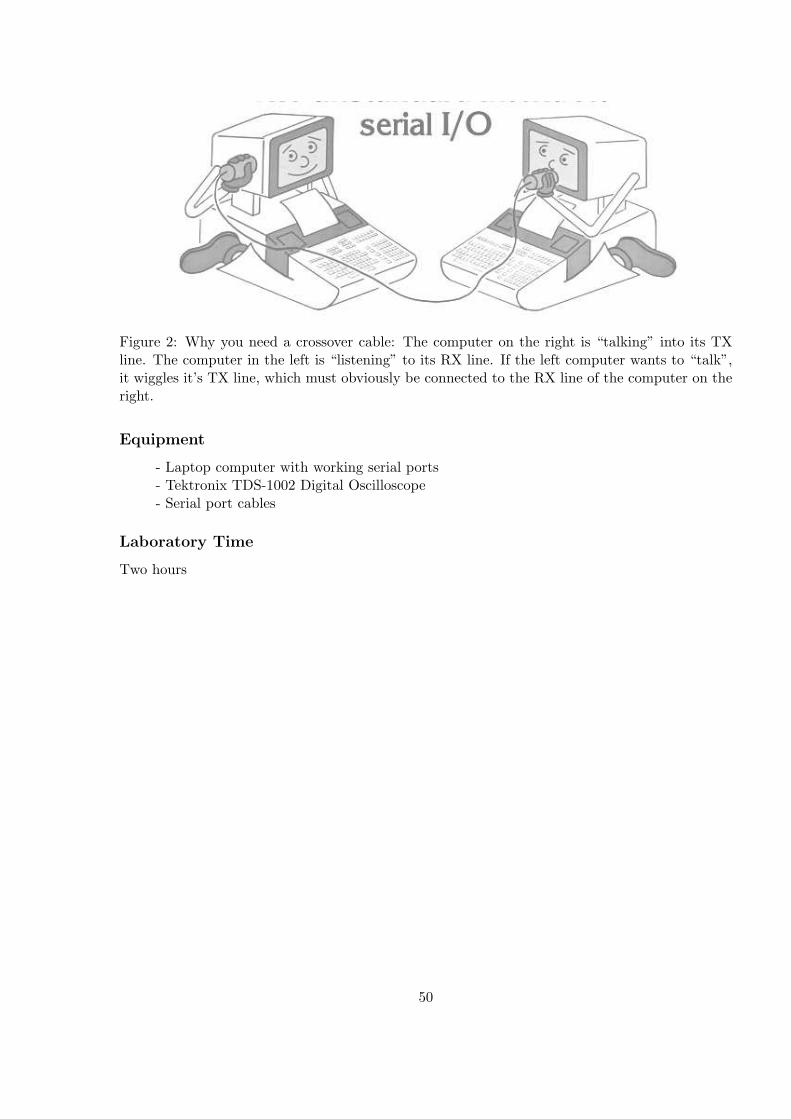
Figure 2: Why you need a crossover cable: The computer on the right is “talking” into its TXline. The computer in the left is “listening” to its RX line. If the left computer wants to “talk”,it wiggles it’s TX line, which must obviously be connected to the RX line of the computer on theright.

Equipment

- Laptop computer with working serial ports- Tektronix TDS-1002 Digital Oscilloscope- Serial port cables

Laboratory Time

Two hours

50

14 Miscellaneous Experiments (n=various!)

Some of these experiments require advance notice because I will have to procure neededsupplies. The amount of notice required is indicated on each.

The following experiments are not completely described. Part of each exercise is to identifythe core scientific objective. Most are n=2 or more because of the work of figuring out what todo and perhaps assemblying supplies. I will help you with these and can decide on their value inadvance.

14.1 Design your own!

This takes one month advance notice because we have to discuss what you will do and obtainmaterials you might need.

Students in this class have tried to design their own transmitter, stereo amplifier, spark gap,or magnetic levitation device. I can help you turn your idea into something that might work.

14.2 Lock-in Amplifiers

This project has a lot of physics and is not lethal. You will build a mechanical ”chopper” anda photo-detector and detect the light from a dim light-bulb in a brightly lit room using lock-intechnology.

14.3 TV remote control

This requires only one week advance notice.Using a phototransistor or photodiode, look at the infrared light signal emitted by a remote

control unit for a television set.

14.4 Resistance and temperature

Requires one week advance notice.Experiment with the following:

1. Thermistor

2. Metal film resistor

3. Carbon resistor

4. Tungsten filament

5. Copper wire

Low temperatures can be produced with liquid nitrogen. You could get some ideas on exper-imental techniques from an article by K. G. Vandervoort, J. M. Willingham, and C. H. Morris(American Journal of Physics, 63(8), 759-760, 1995.

51

14.5 Electric Motors

Requires NO advance notice.If you rotate a motor shaft (say, with another motor) it will generate a voltage. Connect the

shaft of one motor to the shaft of another motor and make measurements to observe the generatedvoltage in both the driving motor and the driven motor.

14.6 Magnetic materials

Requires one month advance notice to order the materials. It should be possible to study themagnetic properties of different types of materials by seeing how they affect the inductance of acoil in an oscillating circuit.

14.7 Electric and magnetic fields of a power line

This takes three weeks advance notice because additional materials must be obtained.An article in Physics Today asks, “Do the all-pervasive low-frequency electromagnetic fields of

modern life threaten our health?” (W. R. Bennett, Jr., Cancer and Power Lines, Physics Today,April 1994, page 23-29.) It might be interesting to measure the electric and/or magnetic fields ofthe biggest power line you can find in the vicinity of Socorro.

14.8 Flames

There is a striking photograph of a flame being pulled toward a Van de Graaff generator in ThePhysics Teacher, vol. 33, page 44, January 1995. It could be interesting to study the electricalproperties of flames. Flames can be used as speakers as well.

14.9 Guitar Pickup

This requires three weeks notice to order the pickups.Electric guitar pickups are beautiful examples of electromagnetic induction. Working through

all the details of the transducer is exciting and educational.

14.10 Build a rail gun

Because it is both dangerous and complex, this project may be undertaken as a paper study.Research rail-guns and write a report that outlines how you would go about building one andwhat physics (B-fields, currents, stresses on the system) you can work out on paper. A paperstudy requires no advance notice and can be good for n=2 for a single person. To actually evenbegin to build one is probably n=5 and we should discuss this by mid-February.

Electromagnetic rail guns can reach very high speeds. This is a wonderful and educationalengineering project in pulsed power and mechanical design. It is also dangerous! I will help you.This should be a group project.

14.11 Build an electromagnetic can crusher

Another good group project that is potentially fatal ... but not until energized. I can guide youthrough the steps needed to charge large capacitors and fire them safely.

Because it is both dangerous and complex, this project may be undertaken as a paper study.Research can-crushers and write a report that outlines how you would go about building one and

52

what physics (B-fields, currents, stresses on the system, forces on the can) you can work out onpaper. A paper study requires no advance notice and can be good for n=2 for a single person.To actually even begin to build one is probably n=5 and we should discuss this by mid-February.

53

Appendices – Data Sheets / Circuits ConceptTest

54