MNRAS 000, 1–12 (2015) Preprint 22 July 2016 Compiled using MNRAS LATEX style file v3.0

A new model of the microwave polarized sky for CMBexperiments

Carlos Hervıas-Caimapo1?, Anna Bonaldi1 and Michael L. Brown1

1Jodrell Bank Centre for Astrophysics, School of Physics & Astronomy, University of Manchester, Oxford Road, Manchester M13 9PL, U.K.

Accepted XXX. Received YYY; in original form ZZZ

ABSTRACTWe present a new model of the microwave sky in polarization that can be used tosimulate data from CMB polarization experiments. We exploit the most recent resultsfrom the Planck satellite to provide an accurate description of the diffuse polarizedforeground synchrotron and thermal dust emission. Our model can include the twomentioned foregrounds, and also a constructed template of Anomalous MicrowaveEmission (AME). Several options for the frequency dependence of the foregroundscan be easily selected, to reflect our uncertainties and to test the impact of differentassumptions. Small angular scale features can be added to the foreground templatesto simulate high-resolution observations.

We present tests of the model outputs to show the excellent agreement with Planckand WMAP data. We determine the range within which the foreground spectral indicescan be varied to be consistent with the current data. We also show forecasts for a high-sensitivity, high-resolution full-sky experiment such as the Cosmic ORigin Explorer(COrE). Our model is released as a python script that is quick and easy to use,available at http://www.jb.man.ac.uk/~chervias.

Key words: methods: data analysis – cosmic background radiation

1 INTRODUCTION

Over the past decades, the temperature anisotropies of theCosmic Microwave Background (CMB) have been an in-valuable probe of the cosmological model (e.g. Hinshawet al. 2013; Calabrese et al. 2013; Planck Collaboration et al.2015a). The design of future CMB experiments is now drivenby the goal of measuring accurately the polarization of theCMB, and searching for primordial polarization B-modes,a detection which would prove unequivocally the inflation-ary scenario. However, bright foreground emission due toour Galaxy can jeopardise this measurement, and accuratemodels of the polarization sky are needed (see, e.g. Betouleet al. 2009; Armitage-Caplan et al. 2012; Errard & Stom-por 2012; Bonaldi et al. 2014; BICEP2/Keck and PlanckCollaborations et al. 2015; Remazeilles et al. 2016).

Until recently, full-sky polarization maps of the Galac-tic emission were based on total intensity measurementsand models of the polarization physical properties, anglesand polarization fractions (e.g. Miville-Deschenes 2011; De-labrouille et al. 2013; O’Dea et al. 2012). However, the uncer-tainties in such modelling made it difficult to create polar-ization templates accurately reproducing the observed mor-

? E-mail: carlos.herviascaimapo@postgrad.manchester.ac.uk

phology in the sky. The recent release of the Planck data hasimproved this situation, by providing for the first time fore-ground maps extracted directly from the polarization data(Planck Collaboration et al. 2015b). Before this informa-tion can be used to forecast future polarization experiments,however, it is necessary to overcome the limitations due tothe Planck resolution and noise levels. Moreover, a suite offoreground models needs to be explored, to reflect the cur-rent uncertainties on polarized foregrounds. This is the goalof the current paper, where we deliver a new sky model ofdiffuse polarized emission in the microwave frequency range,based on the most up-to-date information from Planck.

In contrast to previous work (Delabrouille et al. 2013),the model we present is not a comprehensive model that in-cludes all point-like and diffuse emission in the microwavesky. Instead, we focus on diffuse polarized emission only andaim to provide a simpler and more flexible tool, to allowmodel selection for forecast purposes, as well as to test anddebug data analysis methods on simulated data of varyingcomplexity. We also introduce, for the first time, the capa-bility to vary the foreground morphology for Monte-Carlopurposes. We believe that our model, which we provide as apython script, will be a useful tool for the CMB polarizationcommunity.

The paper is organized as follows: In Sec. 2 we describe

c© 2015 The Authors

arX

iv:1

602.

0131

3v2

[as

tro-

ph.C

O]

21

Jul 2

016

2 Hervıas-Caimapo et al.

-20 20µK

-40 40µK

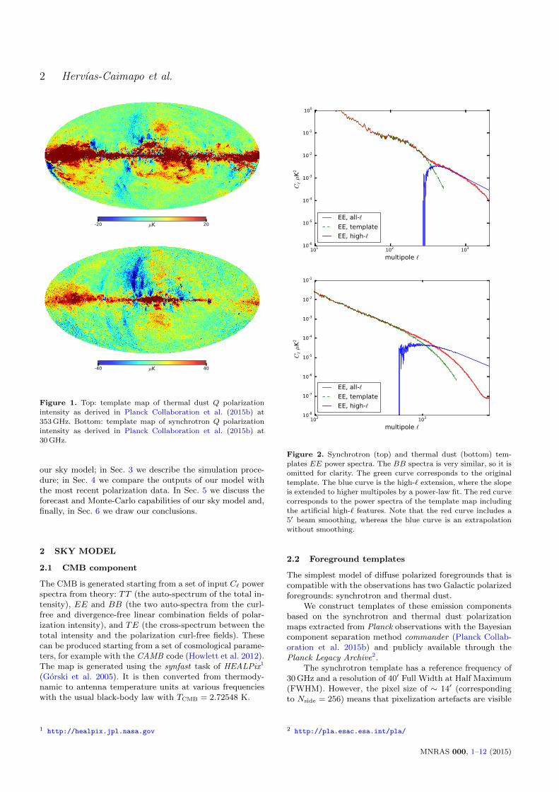
Figure 1. Top: template map of thermal dust Q polarizationintensity as derived in Planck Collaboration et al. (2015b) at

353 GHz. Bottom: template map of synchrotron Q polarization

intensity as derived in Planck Collaboration et al. (2015b) at30 GHz.

our sky model; in Sec. 3 we describe the simulation proce-dure; in Sec. 4 we compare the outputs of our model withthe most recent polarization data. In Sec. 5 we discuss theforecast and Monte-Carlo capabilities of our sky model and,finally, in Sec. 6 we draw our conclusions.

2 SKY MODEL

2.1 CMB component

The CMB is generated starting from a set of input C` powerspectra from theory: TT (the auto-spectrum of the total in-tensity), EE and BB (the two auto-spectra from the curl-free and divergence-free linear combination fields of polar-ization intensity), and TE (the cross-spectrum between thetotal intensity and the polarization curl-free fields). Thesecan be produced starting from a set of cosmological parame-ters, for example with the CAMB code (Howlett et al. 2012).The map is generated using the synfast task of HEALPix1

(Gorski et al. 2005). It is then converted from thermody-namic to antenna temperature units at various frequencieswith the usual black-body law with TCMB = 2.72548 K.

1 http://healpix.jpl.nasa.gov

101 102 103

multipole `

10-6

10-5

10-4

10-3

10-2

10-1

100

C` µK

2

EE, all-`

EE, template

EE, high-`

102 103

multipole `

10-8

10-7

10-6

10-5

10-4

10-3

10-2

10-1

C` µK

2

EE, all-`

EE, template

EE, high-`

Figure 2. Synchrotron (top) and thermal dust (bottom) tem-plates EE power spectra. The BB spectra is very similar, so it is

omitted for clarity. The green curve corresponds to the originaltemplate. The blue curve is the high-` extension, where the slopeis extended to higher multipoles by a power-law fit. The red curve

corresponds to the power spectra of the template map includingthe artificial high-` features. Note that the red curve includes a

5′ beam smoothing, whereas the blue curve is an extrapolation

without smoothing.

2.2 Foreground templates

The simplest model of diffuse polarized foregrounds that iscompatible with the observations has two Galactic polarizedforegrounds: synchrotron and thermal dust.

We construct templates of these emission componentsbased on the synchrotron and thermal dust polarizationmaps extracted from Planck observations with the Bayesiancomponent separation method commander (Planck Collab-oration et al. 2015b) and publicly available through thePlanck Legacy Archive2.

The synchrotron template has a reference frequency of30 GHz and a resolution of 40′ Full Width at Half Maximum(FWHM). However, the pixel size of ∼ 14′ (correspondingto Nside = 256) means that pixelization artefacts are visible

2 http://pla.esac.esa.int/pla/

MNRAS 000, 1–12 (2015)

A new model of the microwave polarized sky 3

1.3 1.7

2.6 3.3

Figure 3. Top: map of thermal dust spectral indices based onPlanck Collaboration et al. (2015b) and smoothed to 3◦ FWHM

to reduce noise. Bottom: map of synchrotron spectral indices

based on Giardino et al. (2002) with βsyn increased to betterfit the Planck frequency range (see text).

on the maps. We eliminated these artefacts by resamplingthe map, upgrading it to Nside = 512 and smoothing it to afinal 1◦ resolution.

The dust template obtained by Planck Collaborationet al. (2015b) has a reference frequency of 353 GHz and aresolution of 10′ FWHM. Figure 1 shows both Q intensitytemplates.

2.2.1 Adding high-` features to the foreground templates

Since the synchrotron and thermal dust templates have finiteresolution, they do not have power at small scales. In ourmodels, we would like to simulate high-` power since the realsky thermal dust and synchrotron emissions are expected tohave these features.

The approach that we follow is to generate a randommap using a suitable power spectrum, based on the extrap-olation of the power spectrum of the original map to highermultipoles. Since this procedure involves a random realiza-tion, it can be also used to create variations over differ-ent foreground maps, for example for Monte Carlo purposes(this aspect is discussed in Sec. 5).

A common assumption is that the power spectrum ofthe foreground maps has a power-law behaviour in `. Fig-ure 2 (top) shows the EE power spectra of the synchrotrontemplate in green. The power-law behaviour is not a good

approximation at the highest multipoles, where the slopeflattens with respect to lower `s. We nonetheless adoptedthe power-law approximation and computed the best-fittingslope at the lowest multipoles. We used a least squares poly-nomial fit, that minimizes the difference between model anddata, added in quadrature within a given multipole range.Our model is a straight line in the logC`–log ` space. Thisprocedure also outputs the covariance matrix for the fit pa-rameters, and we adopted the square root of the diagonalterms as errors on each of them.

For the EE power spectrum, we fitted for the slope inthe multipole interval 10 ≤ ` ≤ 120 and obtained a valueof −1.7 ± 0.04; for the BB power spectrum, we fitted forit in the interval 4 ≤ ` ≤ 40 and obtained a flatter slopeof −1.4 ± 0.05. We obtained power spectra for the high-`features as the difference between the original spectrum andits extrapolation computed using the best-fitting slope. Thisprocedure creates a smooth high-` power spectrum, shownin blue in Fig. 2 (top). After this, we create a realizationmap with the artificial high-` power spectrum, using synfastand using a Gaussian beam appropriate for the resolutionof the simulation.

We finally multiply the resulting random map by anormalized version of the original template map. This re-produces the anisotropy of the foreground map (a Galac-tic plane mask in a sense), where regions in the Galacticplane are typically much brighter than at high latitudes. Thehigh-` random map is finally added to the original template,but multiplied by an amplitude chosen to give a continuouspower spectrum at multipoles corresponding to the originalbeam. The power spectrum of the resulting map (for a 5′

final resolution) is shown in Fig. 2 (top) in red.We follow the same procedure for the dust template.

Fitting for the EE and BB slope in the range 60 ≤ ` ≤ 600yields −2.36±0.005 and −2.16±0.007 respectively. Figure 2(bottom) shows the EE power spectra for the dust template,for a final resolution of 5′. The colour code is the same asin Fig. 2 (top). The slopes of the high-` power spectrum,the beam and the amplitude of the high-` maps are freeparameters of the model and can be chosen to give differentsmall-scale features, as needed for the simulation.

2.3 Baseline foreground model

We model the frequency scaling of the dust and synchrotroncomponents in antenna temperature as:

TA,dust(ν) ∝ νβdust+1[exp(hν/kTd)− 1]−1 (1)

TA,syn(ν) ∝ ν−βsyn , (2)

where h is the Planck constant, k is the Boltzmann constantand ν is the frequency. The parameters Td, βdust and βsyn arethe dust temperature, dust spectral index and synchrotronspectral index, respectively.

The best-fitting values of Planck Collaboration et al.(2015b) are Td = 21 K and a spatially-varying dust spec-tral index with average value 〈βdust〉 = 1.53 over the sky.For the synchrotron component Planck Collaboration et al.(2015b) uses a template spectrum obtained with the GAL-PROP code (Orlando & Strong 2013) instead of a power-law model; the slope of the spectrum between ∼ 19 and∼ 97 GHz corresponds to a βsyn ∼ 3.10. For our baseline

MNRAS 000, 1–12 (2015)

4 Hervıas-Caimapo et al.

model we use spatially-constant parameters derived by thePlanck Collaboration et al. (2015b) analysis: Td = 21 K,βdust = 1.53 and βsyn = 3.10.

2.4 Spatially-varying spectral indices

In order to add complexity to the models, we also consideredusing spatially varying spectral index maps for both dustand synchrotron emission. For thermal dust, we started fromthe map of best-fitting spectral indices calculated using thetemperature Planck maps from commander in Planck Col-laboration et al. (2015b). This map has a resolution of 7.5′

FWHM but it is very noisy. We therefore smoothed it to3◦. The final map of βdust of our model is shown in the toppanel of Fig. 3. For our test model, we do not consider spa-tially varying Td, since there is a degeneracy between βdustand Td. With no ∼THz data, it is very difficult to constrainboth at the same time, so we only consider spatially vary-ing βdust, which has more effect on the spectral law in thefrequency range we consider.

For synchrotron, we use the map of spectral indices byGiardino et al. (2002). This map was derived using the full-sky map of synchrotron emission at 408 MHz from Haslamet al. (1982), the northern-hemisphere map at 1420 MHzfrom Reich & Reich (1986) and the southern-hemispheremap at 2326 MHz from Jonas et al. (1998). The Giardinoet al. (2002) map has a resolution of 10◦.

One possible problem with the Giardino et al. (2002)map is that is was derived at radio frequencies, where thesynchrotron spectral index is typically flatter. We correctedfor this effect by computing the expected steepening between∼ 490–2120 MHz and 20–30 GHz using the same GALPROPtemplate used in the Planck analysis and applying it to theGiardino et al. (2002) map. The result is shown in the bot-tom panel of Fig. 3; the steepening applied is ∆βsyn = 0.13.The mean and standard deviation of this map are 2.9 and0.1, respectively.

2.5 Curved synchrotron spectral index andmultiple thermal dust components

There is evidence that the synchrotron spectral law is not aconstant power-law, instead having a curvature as the fre-quency increases (Kogut 2012). In order to model this, wereplace equation 2 by

TA,syn(ν) ∝ (ν/ν0)−βsyn+C log(ν/νpiv), (3)

where C is the curvature amplitude, ν0 is the referencefrequency of the synchrotron template and νpiv is a pivotfrequency. Positive values of C flatten, and negative onessteepen the spectral law for increasing frequency. For ex-ample, Kogut et al. (2007) finds a slight flattening of thespectrum with C ∼ 0.3 for νpiv = 23 GHz for WMAP data.

The thermal dust spectral law might be better modelledusing more than one modified black body, (e.g., Finkbeineret al. 1999; Meisner & Finkbeiner 2015). The physical moti-vation is that different types of dust grains would be charac-terised by a different emission law. For this reason, we allowan arbitrary number of components, provided the user spec-ifies βdust (or a map of coordinate-dependent βdust), Td, and

-4 4µK

Figure 4. Template map of Q AME component, as derived from

the total intensity AME and the thermal dust polarization mapsfrom Planck Collaboration et al. (2015b). This map has 1◦ resolu-

tion, a reference frequency of 23 GHz and assumed a polarization

fraction of 0.01.

an amplitude Edust for each component. We replace equa-tion 1 with

TA,dust(ν) ∝Nmbb∑i=1

Edust,i νβdust,i+1[exp(hν/kTd,i)− 1]−1,

(4)

where Nmbb is the number of modified black body compo-nents. We note that our parameterisation is equivalent tothat in Meisner & Finkbeiner (2015) once our Edust,i is theirfiqi. In that work, qi is a physical parameter describing thedust component, specifically the ratio of far-infrared emis-sion cross-section to optical absorption cross-section. Theparameter fi is the relative contribution (or fraction) of eachcomponent to the total (normalized such that

∑Nmbbi fi =

1). Our amplitude parameter Edust,i accounts for both, andit is therefore a phenomenological, rather than a physical,parameter. For example, the best-fitting model (model 8)of Finkbeiner et al. (1999) has two modified black bodycomponents that, in our parametrization, are described byTd,1 = 9.4 K, βd,1 = 1.67, Td,2 = 16.2 K, βd,2 = 2.70, andintensity ratios Edust,1/Edust,2 = 0.49.

2.6 Additional polarized components: AnomalousMicrowave Emission (AME)

There is evidence that AME due to spinning dust is polar-ized, with a polarization fraction of few % (Dickinson et al.2011; Genova-Santos et al. 2015). We consider the polar-ization intensity of the AME as an additional feature tosimulate observations by future experiments with a betteraccuracy.

To construct our AME template we used the Planck2015 total intensity AME template (with a resolution of 1◦)and the thermal dust polarization maps. By assuming thatthe polarization angles for AME are the same as for thethermal dust, we can obtain polarization Q and U maps forAME as

QAME = fp,AME TAME cos(2χTD) (5)

UAME = fp,AME TAME sin(2χTD), (6)

MNRAS 000, 1–12 (2015)

A new model of the microwave polarized sky 5

Figure 5. Scatter plot inside the Galactic plane |b| ≤ 20◦. The Nside is 64. The top row corresponds to Q intensity, and the bottom

row to U intensity. The black line represents the perfect one-to-one match. Both the templates and the observed sky were smoothed toa common 1◦ resolution.

where fp,AME is a spatially-constant polarization fraction(we used a default value of 1%), TAME is the total inten-sity AME template, and χTD is the thermal dust polariza-tion angle. The Pearson correlation coefficient between thethermal dust and the AME template (at 1◦ resolution andNside = 64) is 0.71±0.01 (Q map) and 0.73±0.01 (U map).The errors were calculated with jackknife resampling. Figure4 shows the Q intensity of the constructed AME template,with a reference frequency of 23 GHz.

As a spectral law, we adopt a parabola in the logarith-mic flux-frequency space, proposed by Bonaldi et al. (2007),given by

log(TA,ν) = const.−[

m60 log(νmax)

log(νmax/60GHz)+ 2

]log(ν)+

m60

2 log(νmax/60GHz)(log(ν))2, (7)

where the free parameters are m60 (the slope at 60 GHz)in the log(ν)-log(S) space, and νmax is the peak frequency(for the spectrum in flux units). We adopt as default values

νmax = 19 GHz, from Planck Collaboration et al. (2015b),and 4.0 for m60 from Bonaldi et al. (2007).

2.6.1 Adding dust-correlated high-` features to the AMEmaps

Similarly to what done for the synchrotron and thermal dustcomponents in Sec. 2.2.1, the AME polarization maps can beupgraded in resolution by adding high-` features. However,in this case we want the high-` thermal dust and AME mapsto exhibit the same level of correlation measured at low res-olution. We therefore developed a special procedure for thiscase, that generates both dust and AME high-` correlatedrandom maps at the same time.

We followed the procedure described in Brown & Battye(2011), which uses as input the spectra and cross-spectraof the set of correlated maps (in our case, dust E and B,and AME E and B). This information is used to generate 4correlated a`m fields, which are finally transformed to Q andU with the HEALPix alm2map function. Extending what isdescribed in Sec. 2.2.1, the spectra and cross-spectra for the

MNRAS 000, 1–12 (2015)

6 Hervıas-Caimapo et al.

high-` maps are constructed by extrapolating those of thedust and AME templates to higher multipoles. The last stepof our procedure, the modulation of the random high-` mapswith a mask enhancing the Galactic plane, is unchanged.

3 SIMULATED OBSERVATIONS OF CMBPOLARIZATION EXPERIMENTS

3.1 Simulating the instrumental response

To simulate the observation of the microwave sky in polar-ization by a given experiment, we need to know the fre-quency bands of observation and, for each of the bands,the point-spread function and the noise level. Each of theseproperties can be simulated with different level of complex-ity, specified by the user, as detailed in the following.

The frequency response can be either simulated as adelta function (monochromatic response) or a more generaltransmission. In the more general case, the intensity of thesky component i at the frequency band νj is given by:

Ti(νj) =

∑kWj(νk)[Q/U ]refSi(νk)∑

kWj(νk), (8)

where Si(ν) is the spectral law of the component, [Q/U ]refis the Q or U amplitude of the corresponding template, andWj(νk) is the transmission of band j for a set of frequenciesνk. In practice, when simulating a band response, the signalneeds to be simulated for a set of frequencies νk and averagedover the entire band, with weights given by the transmissionWj(νk).

The effect of the instrumental resolution is simulatedby convolving the maps with a Gaussian beam of specifiedFWHM.

The noise can be modelled either as a uniform whitenoise, described by a unique rms value over all the sky, or asan anisotropic white noise specifying a map of rms varyingin the sky. For Planck, we model this using the 3 × 3 noisecovariance per pixel containing the Stokes parameter covari-ance elements TT , QQ, UU , TQ, TU , and QU . In this case,for each pixel, a Cholesky decomposition is performed overthe covariance matrix; the diagonal elements of the decom-position finally yield the standard deviations per pixel forT , Q, and U , respectively.

3.2 Simulation procedure

Once the experiment is specified, by means of a set of fre-quencies, resolution and noise, the simulation procedure isthe following:

• A CMB map is generated using synfast, up to a res-olution equal to θ∗, which should be at least equal to thesmallest instrumental beam of the experiment.• High-` features are optionally added to the synchrotron,

dust and/or AME templates up to a resolution θ∗ (if θ∗ issmaller than the intrinsic resolution of the template).• The CMB map and foreground templates are scaled

in intensity according to the frequency behaviour to eachfrequency band, added together and smoothed to match theresolution appropriate for that channel.

• A noise map is generated and added to the frequencyband for each channel to obtain the simulated frequencymap.

The outputs are the frequency maps, but also the com-ponent maps at all required frequencies. Some of the compo-nents can be easily deactivated to obtain noise-only, signal-only, foreground-only or CMB-only simulations, for examplefor Monte Carlo purposes.

4 COMPARISON WITH DATA FROM PLANCKAND WMAP

4.1 Foreground model

For the comparisons shown in this section we used the base-line foreground model described in Sec. 2.3. This includessynchrotron and thermal dust with fixed spectral indices inthe sky. We do not include the polarized AME component,that was not detected by Planck due to its weakness com-pared to the noise levels (Planck Collaboration et al. 2015b).

4.2 Data maps

We compared the output of our model with Planck sky ob-servations in polarization at 30, 44, 70 and 353 GHz, com-plemented by the WMAP W band at 94 GHz and K bandat 23 GHz. In the following, we carried out the comparisonbetween model and data smoothing to a 1◦ common reso-lution, which is the resolution of our synchrotron template.Such resolution is also good for display purposes because itreduces the noise and allows an easier visual inspection ofthe foregrounds morphology.

The Planck frequency maps have been corrected for thepolarization leakage due to bandpass mismatch with the cor-rection maps available on the Planck Legacy Archive. TheWMAP maps have been downloaded from the LAMBDA-WMAP archive 3.

4.3 Comparison with foregrounds only

We first compared the data with a model of the sky includingonly the foregrounds (with no high-` features) and withoutCMB and noise. In this way, we only compare the determin-istic components of the model, without any random realiza-tion. The true Planck and WMAP frequency responses havebeen used to create the model sky as described in Sec. 3.

Figure 5 shows a pixel-by-pixel comparison of true vsmodel Q and U maps. We show only the pixels inside theGalactic plane (|b| ≤ 20◦) for Nside = 64 to reduce theeffect of noise and CMB. Figure 6 shows the maps in pseudo-colour scale, for 6 frequencies and in Q and U intensity. Themodelled foregrounds and the observed sky have the samecolour scale. As expected, the agreement is very good forthe foreground-dominated frequencies. At 70 and 94 GHzthe agreement is less good, because CMB and noise becomeimportant. The direct comparison of the maps shows thatthe foreground model is quite good once the noise is reduced(by means of degrading to Nside = 32). The U intensity

3 http://lambda.gsfc.nasa.gov/product/map/dr5/

MNRAS 000, 1–12 (2015)

A new model of the microwave polarized sky 7

Sky 2360453015

015304560

Model 2360453015

015304560

Sky 305040302010

01020304050

Model 305040302010

01020304050

Sky 4420161284

048121620

Model 4420161284

048121620

Sky 7020161284

048121620

Model 7020161284

048121620

Sky 9420161284

048121620

Model 9420161284

048121620

Sky 35360453015

015304560

Model 35360453015

015304560

Sky 23302418126

0612182430

Model 23302418126

0612182430

Sky 30252015105

0510152025

Model 30252015105

0510152025

Sky 44108642

0246810

Model 44108642

0246810

Sky 70108642

0246810

Model 70108642

0246810

Sky 94108642

0246810

Model 94108642

0246810

Sky 353302418126

0612182430

Model 353302418126

0612182430

Figure 6. Maps comparison between the observed sky and the foreground model. Left: maps for Q intensity. Right: maps for U intensity.

The rows are six bands, the left column corresponds to the observed sky and the right one to our foregrounds model. The units are µKA.The maps are smoothed to a common 1◦ resolution and degraded to Nside = 32 to suppress the noise for display purposes.

of the 94 GHz band is noisy, which makes the comparisondifficult.

4.4 Including the contribution from noise andCMB

For the comparisons presented in this section, we includednoise and a CMB realization, which are present in the skyobservations, in order to assess the match of the model whenall components are included. In this case we only considerthe power spectra, since the different CMB and noise real-izations do not allow a morphological comparison.

The CMB map has been generated starting from thebest-fitting model of Planck (including polarization informa-tion, Planck Collaboration et al. (2015a)) and with tensor-to-scalar ratio r = 0.1.

In this case, we consider the 30, 44, 70, and 353 GHzPlanck bands and all five of the WMAP bands. The WMAPnoise is simulated using the hit counts maps and RMS in-formation available from the Lambda website. Planck noisehas been simulated using the pixel covariance information.However, this noise is based on the Planck data before ap-plying the leakage correction maps, while the data used forthe comparison has the correction applied. As illustratedfor 70 GHz in Fig. 9, the bandpass correction subtracts alarge fraction of the noise, therefore the noise contributionat small scales is over-estimated. For this reason, the com-parison that follows is limited to ` ≤ 100 where this effect isnot significant.

Figure 7 shows the comparison of the EE and BBfull-sky power spectra between the complete model (fore-grounds model + noise realization + CMB realization) andthe Planck bands. Figure 8 shows the same for the fiveWMAP bands. Since these spectra are computed over thefull-sky, there is no leakage between EE and BB modes andno correction is needed. In this case, the error on the datapower spectrum (orange shaded region) is just due to noiseand CMB variance, and is calculated as

∆C` =

√2

2`+ 1(CCMB

` +N`), (9)

where CCMB` is the input CMB power spectrum andN` is the

noise bias power spectrum, calculated from 100 noise MonteCarlo realizations based on the noise covariance matrix in-formation of each band. This error is generally very smallcompared to the foreground signal (< 1%), and in most casesnot visible in the figures. The maximum observed error, con-sidering multipoles up to ` = 100, is ∼ 10% at 70 GHz forPlanck and ∼ 23% at 61 GHz for WMAP.

The agreement between the intermediate frequencies(44 and 70 GHz) benefits from the inclusion of CMB andnoise in the comparison. At 70 GHz the CMB polarised in-tensity is strong, so the match improves. The inclusion ofnoise is particularly important to reconcile model and datatowards ` = 100.

MNRAS 000, 1–12 (2015)

8 Hervıas-Caimapo et al.

101

102

EE 30 GHz BB 30 GHz

100

101

EE 44 GHz BB 44 GHz

10-1

100

101

EE 70 GHz BB 70 GHz

101 102

101

102

EE 353 GHz

101 102

BB 353 GHz

multipole `

`(`+

1)C`/

2π µ

K2 A

Figure 7. EE (left) and BB (right) full-sky power spectra com-

parison between the complete model (foregrounds+noise+CMB,

in green) and the observed sky (in orange) in four Planck bands,for Nside = 256. The error for the observations is plotted as the

orange shaded region. The full-sky maps are smoothed to a com-

mon 1◦ resolution.

4.4.1 Comparison on small patches at high Galacticlatitude

As a final assessment of our model, we compare local powerspectra to the latest Planck observations in several small skypatches at intermediate and high Galactic latitude. This isparticularly useful for ground-based CMB polarization ex-periments, which target these areas. For example, the BI-CEP2/KECK array (BICEP2 Collaboration et al. 2014) ob-serves with two bands at 100 and 150 GHz. They target ahigh Galactic latitude patch visible from the South Pole,with a size of ∼ 800 deg2. The South Pole Telescope (SPT)has measured the sub-degree scales lensing BB power spec-trum in a southern 100 deg2 patch using two bands (95 and150 GHz) (Keisler et al. 2015). Another example is the PO-LARBEAR experiment, in the Atacama desert in Chile,which measured the lensing BB spectrum in three smallpatches with a total area of 25deg2 at 150 GHz (The Po-larbear Collaboration: P. A. R. Ade et al. 2014). Given thefrequency coverage of these experiments, observing around150 GHz, where the CMB peaks, it is crucial to model cor-

102

103

EE 23 GHz BB 23 GHz

101

102

EE 33 GHz BB 33 GHz

100

101

EE 41 GHz BB 41 GHz

10-1

100

101

EE 61 GHz BB 61 GHz

101 102

10-1

100

101

EE 94 GHz

101 102

BB 94 GHz

multipole `

`(`+

1)C`/

2π µ

K2 A

Figure 8. EE (left) and BB (right) full-sky power spectra com-

parison for the five WMAP bands. The error for the observationsis plotted as the orange shaded region. The full-sky maps are

smoothed to a common 1◦ resolution. The convention is the same

as in Fig. 7.

101 102 103

multipole `

10-7

10-6

10-5

10-4

10-3

10-2

10-1

100

101

102

103

`(`+

1)C`/

2π µ

K2

Planck sky bp correctedNoise realisationPlanck sky NOT bp corrected

Figure 9. Full-sky BB power spectra with Nside = 256 for boththe Planck sky maps at 70 GHz before (red) and after (blue) band-pass leakage correction. A noise realization (green) agrees well at

high-`, but since the bandpass leakage correction affects the noise,there is no agreement anymore with the noise level.

MNRAS 000, 1–12 (2015)

A new model of the microwave polarized sky 9

0.0 0.5 1.0 1.5 2.0

AXX for sky model µK2353GHz

0.0

0.5

1.0

1.5

2.0

AX

X f

or

sky o

bse

rvati

ons µK

2 353G

Hz

AEE

ABB

3.5 3.0 2.5 2.0 1.5 1.0 0.5 0.0 0.5 1.0

αXX for sky model

3.5

3.0

2.5

2.0

1.5

1.0

0.5

0.0

0.5

1.0

αX

X f

or

sky o

bse

rvati

ons

αEE

αBB

Figure 10. Correlation of the fitted power-law between ourmodel and Planck 353 GHz observations for several intermediateand high latitude small patches. Top, correlation for the value ofthe amplitude AXX at ` = 80. The stars corresponds to the BI-CEP2 field. Bottom, correlation between the values of the power-

law slope αXX .

rectly the contamination from polarized thermal dust emis-sion.

For our comparison, we followed a similar procedure tothe one described in Planck Collaboration et al. (2016) forassessing the contamination by thermal dust. We produceddisk-shaped masks with a radius of 11.3◦ (400 deg2). Eachpatch is located on the center of a pixel of a Nside = 8map and we considered patches whose center has a lati-tude of |b| > 45◦. This leaves 48 circular patches. We alsoadded another mask that selects the region targeted by BI-CEP2/KECK. The masks are apodized by smoothing witha 2◦ FWHM beam.

0.5 1.0 1.5 2.0 2.5

βdust

1.5

2.0

2.5

3.0

3.5

4.0

βsy

n

0.5 1.0 1.5 2.0 2.5

βdust

1.5

2.0

2.5

3.0

3.5

4.0

βsy

n

0.0

0.1

0.2

0.3

0.4

0.5

0.6

0.7

0.8

0.9

1.0

Norm

aliz

ed p

robabili

ty

0.0

0.1

0.2

0.3

0.4

0.5

0.6

0.7

0.8

0.9

1.0

Norm

aliz

ed p

robabili

ty

Figure 11. Normalized probability for βdust and βsyn obtained

by adding the χ2 values for two Planck bands: 44+70 GHz. Inthis case, the pixels inside a Galactic latitude b ± 20◦ are used.

The black curve represents the 1σ confidence interval. The left

panel shows the constraints given by Q maps, and the right onethose given by U maps.

We used the same maps assessed in Fig. 7 (Nside = 256,1◦ FWHM resolution, modelled as foregrounds + noise +CMB). On each small patch, we calculated the pseudo-C`for both our model and the Planck observations at 353 GHz,in order to compare the thermal dust polarization inten-sity. Then, we corrected for the effect of masking with apseudo-C` approach (e.g., Brown et al. 2005). FollowingPlanck Collaboration et al. (2016), we fitted for the powerlaw DXX

` = AXX(`/80)αXX+2, where XX is either EE orBB, using the same fitting method described in Sec. 2.2.1over a range of multipoles ` = 40–100.

To assess the match, we plot the fitted AXX and αXXfrom the model and from Planck 353 GHz observations inFig. 10. The crosses represent each one of the disk-shapedpatches, while the star represents the BICEP2 field for eitherEE or BB. The agreement is better on the foreground am-plitude AXX than on the slope αXX , our model being gener-ally a bit steeper than the Planck 353 GHz channel. For thepatches having lowest signal, the mismatch is mostly due toerrors in modelling the noise, as detailed in Fig. 9. For thesignal-dominated patches, the mismatch is more likely dueto foreground modelling. The Planck commander analysisthat produced the templates was optimized for the full-skyrather than a small sky patch. As a consequence, the matchon individual 400 deg2 sky areas may vary, but there is agood agreement when considering a sample of sky patches.

4.5 Optimal spectral index test

In the previous tests, we used the best fit values for thespectral indices βsyn = 3.10 and βdust = 1.53, according toPlanck Collaboration et al. (2015b). We might wonder if thisis the optimal choice. Here, we explore the possibility thatchanging the spectral index of synchrotron and/or dust mayimprove the match. This analysis will also provide indica-tions of what is a reasonable range within which to varythe synchrotron and dust spectral indices, for example forMonte Carlo purposes, while preserving a good agreementwith the data.

MNRAS 000, 1–12 (2015)

10 Hervıas-Caimapo et al.

We do this by defining a χ2 statistic in the pixel do-main. The sky observations and the model, with a commonresolution of 1◦, are degraded to Nside = 64. Then, we com-pare the maps pixel by pixel, using as the σ error the Plancknoise maps discussed in Sec. 3.1, properly smoothed and de-graded. Therefore, for an observed band ν, we minimize

χ2ν(βdust, βsyn) =

Npix∑i=0

(Qi,ν −Qi,model(βdust, βsyn))2

(σQi,ν)2, (10)

and analogous for U , where i cycles through the Npix pixelsof the map being considered.

We mapped the χ2 values for a grid of (βdust, βsyn)parameters and for both the 70 and 44 GHz bands. Wecould not use the Planck 30 and 353 GHz because thoseare the frequencies at which the synchrotron and dust tem-plates are normalized, therefore are unaffected by changingthe spectral indices. Also, we did not consider the WMAPchannels because of their higher noise levels. We finally ob-tained a joint likelihood for the 44 and 70 GHz channels asexp(−χ2/2), where χ2 = χ2

44GHz + χ270GHz.

In Figure 11 we show the results for the pixels insidea b = ±20◦ Galactic strip. The left panel corresponds tothe Q maps, the right one to the U maps. The black curvecorresponds to the 1σ confidence interval in the βdust-βsynspace considered. Notice that we assume a prior on the rangeof values these indices can take. The probability distributionis flatter in U (and therefore the 1σ contour is wider) becausethe U maps have weaker foreground emission, as can be seenin Fig. 6.

The best fit values for the 1D marginalized probabilityof each parameter and its 1σ confidence interval, addingboth bands and both polarizations (44+70 GHz and Q+U),are βsyn = 3.4+0.7

−0.5 and βdust = 1.6+0.5−0.2 for the pixels inside

the Galactic plane strip, and βdust = 1.6+0.6−0.3 and βsyn =

3.4+0.9−0.6 when we consider the full-sky. The reason why we

obtain relatively weak constraints is because we could onlyuse data at central frequencies, where foregrounds are not sostrong and the two spectral indices are more degenerate. Atest of the model with much lower (higher) frequency wouldgive a much stronger constraint of the synchrotron (dust)spectral index.

5 FORECAST AND MONTE-CARLOCAPABILITIES

To illustrate the simulation capabilities of our sky model weconsider the specifications of the Cosmic Origin Explorer(COrE) experiment described in The COrE Collaborationet al. (2011). The instrumental specifications are reportedin Table 1. This experiment has 15 frequency bands withfrequency ranging from 45 to 795 GHz and resolution of 23–1.3 arcminutes. The noise is simulated as Gaussian and uni-form, with standard deviation of a few µK per arcminute,as quoted in the Table.

Figure 12 shows the forecasted B-mode for foregroundsfor COrE as obtained with our sky model. The CMB BBpower spectra for different tensor-to-scalar ratios are com-pared with the foreground power at three COrE frequencies:45, 105 and 315 GHz. The foreground power spectra havebeen computed with the WMAP polarization mask (exclud-ing ∼ 37% of the sky); it has been corrected for again using

101 102 103

multipole `

10-12

10-11

10-10

10-9

10-8

10-7

10-6

10-5

10-4

10-3

`(`+

1)CBB

`/2π m

K2

Prim. r=0.1

Prim. r=0.01

Prim. r=0.001

G. Foregrounds 45 GHz

G. Foregrounds 105 GHz

G. Foregrounds 315 GHz

Figure 12. Forecast for primordial BB modes detectability. Theblack curves show primordial CBB` for three values of the tensor-

to-scalar ratio. We also show the BB power spectra for polar-ized foregrounds for three frequencies: 45, 105, and 315 GHz. The

foreground maps were masked with the WMAP polarization data

analysis mask and deconvolved from pseudo-C` following Brownet al. (2005).

15

20

25

30

35

40

45CMB COrE simulation, 45 GHz

165 170 175 180 185 190 19515

20

25

30

35

40

45COrE simulation, 105 GHz

170 175 180 185 190 195

COrE simulation, 315 GHz

10

8

6

4

2

0

2

4

6

8

10

Q Inte

nsi

ty µK

G. Longitude

G.

Lati

tude

Figure 13. Zoomed-in region of intermediate foreground con-

taminations in a simulation of COrE observations. The maps arepatches of Q intensity, 30◦×30◦, centred at l = 180◦, b = +30◦.The top left panel shows a CMB realization (in thermodynamic

units), and the remaining panels show the simulated observationsfor three frequencies: 45 GHz (dominated by synchrotron emis-

sion), 105 GHz (dominated by CMB), and 315 GHz (dominated

by thermal dust emission). These panels have Antenna units.

MNRAS 000, 1–12 (2015)

A new model of the microwave polarized sky 11

Band [GHz] 45 75 105 135 165 195 225 255 285 315 375 435 555 675 795

Beam FWHM [arcmin] 23.3 14.0 10.0 7.8 6.4 5.4 4.7 4.1 3.7 3.3 2.8 2.4 1.9 1.6 1.3

Noise [µK·arcmin] 8.61 4.09 3.5 2.9 2.38 1.84 1.42 2.43 2.94 5.62 7.01 7.12 3.39 3.52 3.60

Table 1. Reference values used for simulating COrE observations.

the pseudo-C` approach of Brown et al. (2005). Althoughthis figure is qualitatively similar to other forecasts in theliterature (e.g. The COrE Collaboration et al. 2011), thefact that our model is based on actual polarization observa-tions ensures a better match with the real sky and thereforeimproved forecast capabilities.

In Fig. 13 we show the Q intensity on a 30◦×30◦ skypatch located at l = 180◦, b = 30◦ and exhibiting interme-diate foreground contamination. The top left panel showsa CMB realization with 4′ resolution. The remaining pan-els show the simulated COrE observations in this regionat 45 GHz, dominated by synchrotron emission, 105 GHz,dominated by CMB emission, and 315 GHz, dominated bythermal dust emission. The resolution in each panel is dif-ferent and corresponds to the COrE resolution quoted inTable 1. The features of the foreground components are eas-ily viewed. On the smallest scales, the foregrounds struc-tures are those generated with the procedure described inSec. 2.2.1, which allows overcoming the limits imposed bythe intrinsic resolution of the templates (1◦ for synchrotronand 10′ for thermal dust).

As mentioned, a valuable feature of our sky model isthe capability to randomize to a certain degree the polar-ized foreground components, for example for Monte-Carlopurposes. This can be particularly useful to produce sim-ulations that reflect our uncertainties on the polarizationof the foregrounds. The randomization method exploits thesame procedure described in Sec. 2.2.1 to upgrade the reso-lution of the templates. By changing the parameters describ-ing the power spectrum of the high-` map (such as the slopeand normalization), it is possible to obtain fainter/strongerforeground contamination at intermediate and small scales.Moreover, by changing the seed of the random realization, itis possible to obtain independent patterns for the same con-figuration. This is illustrated in Fig. 14, where we show theQ intensity for the synchrotron emission in a 5◦×5◦ patchof the sky centered in the same coordinates as Fig. 13. Thetop panels show the original synchrotron emission templateat 1◦ resolution on the left and a high-resolution (5′) oneon the right. The bottom panels show two alternative ver-sions of the top-right panel: a different realization with thesame power spectrum on the left and the same random real-ization with steeper power spectrum (and therefore fainterforeground features) on the right.

6 CONCLUSIONS

We have constructed and validated a new model of themicrowave sky in polarization, based on the most recentresults from the Planck experiment (Planck Collaborationet al. 2015c). Our model features multiple choices for thefrequency-dependence of the polarized synchrotron and dust

27

28

29

30

31

32

33Original template Added high-`

177 178 179 180 181 182 18327

28

29

30

31

32

33Added high-`, different seed

178 179 180 181 182 183

Added high-`, different C` power law

20

16

12

8

4

0

4

8

12

16

20

Q Inte

nsi

ty µK

G. Longitude

G.

Lati

tude

Figure 14. Illustration of the foregrounds randomization capa-

bilities of the code on a 5◦×5◦ sky patch centred at l = 180◦,b = 30◦. The top left panel shows the original Q synchrotrontemplate, which has a FWHM of 1◦; the top right panel shows

the same template upgraded in resolution to 5′ by adding high-`features. The bottom left panel shows the same as the top right,

but with a different random realization. The bottom right panel

shows the same as the top right one, but with a steeper powerspectrum at high multipoles (and therefore fainter foreground fea-

tures).

foregrounds of increasing complexity. The templates, basedon the Planck observations, are upgraded in resolution bymeans of a random map modulated by the large-scale fore-ground emission. This allows simulating experiments withhigher resolution than Planck. At the same time, it allowsrandomizing over the small-scale foreground features, for ex-ample in a Monte-Carlo approach. We also include curvaturein the synchrotron spectral law, and the capability to modelan arbitrary number of modified black bodies for the ther-mal dust law. Finally, we include the choice of a polarizedAME emission template, constructed from the thermal dustpolarization angles and from the AME total intensity tem-plate provided by Planck.

We demonstrated that our baseline model (power-lawsynchrotron with fixed spectral index βsyn = 3.10, modifiedblackbody thermal dust with fixed temperature Td = 21 Kand spectral index βdust = 1.53) gives a very good matchwith both WMAP and Planck data. We also found goodagreement between the dust model and the data on small

MNRAS 000, 1–12 (2015)

12 Hervıas-Caimapo et al.

high-latitude regions, typically targeted by ground-based ex-periments. When changing the parameters of the model,βsyn = 2.9 − 4.2 and βdust = 1.4 − 2.1 also provide a goodfit to the data.

We finally showed the capabilities of our model for fore-cast and Monte-Carlo purposes by simulating data for theCOrE experiment. Our easy to use python package, whichwe make fully available4, will be a useful tool for the CMBpolarization community.

ACKNOWLEDGEMENTS

CHC acknowledges the funding from BecasChile/CONICYT. AB and MLB acknowledge supportfrom the European Research Council under the EC FP7grant number 280127. MLB also acknowledges supportfrom an STFC Advanced/Halliday fellowship. We gratefullyacknowledge the anonymous referee for useful suggestionsthat led to the improvement of this paper.

REFERENCES

Armitage-Caplan C., Dunkley J., Eriksen H. K., Dickinson C.,

2012, MNRAS, 424, 1914

BICEP2 Collaboration et al., 2014, ApJ, 792, 62

BICEP2/Keck and Planck Collaborations et al., 2015, PhysicalReview Letters, 114, 101301

Betoule M., Pierpaoli E., Delabrouille J., Le Jeune M., Cardoso

J.-F., 2009, A&A, 503, 691

Bonaldi A., Ricciardi S., Leach S., Stivoli F., Baccigalupi C., de

Zotti G., 2007, MNRAS, 382, 1791

Bonaldi A., Ricciardi S., Brown M. L., 2014, MNRAS, 444, 1034

Brown M. L., Battye R. A., 2011, MNRAS, 410, 2057

Brown M. L., Castro P. G., Taylor A. N., 2005, MNRAS, 360,

1262

Calabrese E., et al., 2013, Phys. Rev. D, 87, 103012

Delabrouille J., et al., 2013, A&A, 553, A96

Dickinson C., Peel M., Vidal M., 2011, MNRAS, 418, L35

Errard J., Stompor R., 2012, Phys. Rev. D, 85, 083006

Finkbeiner D. P., Davis M., Schlegel D. J., 1999, ApJ, 524, 867

Genova-Santos R., et al., 2015, MNRAS, 452, 4169

Giardino G., Banday A. J., Gorski K. M., Bennett K., Jonas J. L.,

Tauber J., 2002, A&A, 387, 82

Gorski K. M., Hivon E., Banday A. J., Wandelt B. D., HansenF. K., Reinecke M., Bartelmann M., 2005, ApJ, 622, 759

Haslam C. G. T., Salter C. J., Stoffel H., Wilson W. E., 1982,A&AS, 47, 1

Hinshaw G., et al., 2013, ApJS, 208, 19

Howlett C., Lewis A., Hall A., Challinor A., 2012, J. Cosmology

Astropart. Phys., 4, 27

Jonas J. L., Baart E. E., Nicolson G. D., 1998, MNRAS, 297, 977

Keisler R., et al., 2015, ApJ, 807, 151

Kogut A., 2012, ApJ, 753, 110

Kogut A., et al., 2007, ApJ, 665, 355

Meisner A. M., Finkbeiner D. P., 2015, ApJ, 798, 88

Miville-Deschenes M., 2011, in Bastien P., Manset N., ClemensD. P., St-Louis N., eds, Astronomical Society of the Pacific

Conference Series Vol. 449, Astronomical Polarimetry 2008:

Science from Small to Large Telescopes. p. 187

O’Dea D. T., Clark C. N., Contaldi C. R., MacTavish C. J., 2012,

MNRAS, 419, 1795

4 at http://www.jb.man.ac.uk/~chervias

Orlando E., Strong A., 2013, MNRAS, 436, 2127

Planck Collaboration et al., 2015c, preprint, (arXiv:1502.01585)Planck Collaboration et al., 2015b, preprint, (arXiv:1502.01588)

Planck Collaboration et al., 2015a, preprint, (arXiv:1502.01589)

Planck Collaboration et al., 2016, A&A, 586, A133Reich P., Reich W., 1986, A&AS, 63, 205

Remazeilles M., Dickinson C., Eriksen H. K. K., Wehus I. K.,

2016, MNRAS, 458, 2032The COrE Collaboration et al., 2011, preprint,

(arXiv:1102.2181)

The Polarbear Collaboration: P. A. R. Ade et al., 2014, ApJ, 794,171

This paper has been typeset from a TEX/LATEX file prepared by

the author.

MNRAS 000, 1–12 (2015)