Experiments and modelling for by-pass pigging of pipelines
179
Delft University of Technology Experiments and modelling for by-pass pigging of pipelines Hendrix, Maurice DOI 10.4233/uuid:3b3856c6-9eac-4599-be8b-b64fe73e5a5a Publication date 2020 Document Version Final published version Citation (APA) Hendrix, M. (2020). Experiments and modelling for by-pass pigging of pipelines. https://doi.org/10.4233/uuid:3b3856c6-9eac-4599-be8b-b64fe73e5a5a Important note To cite this publication, please use the final published version (if applicable). Please check the document version above. Copyright Other than for strictly personal use, it is not permitted to download, forward or distribute the text or part of it, without the consent of the author(s) and/or copyright holder(s), unless the work is under an open content license such as Creative Commons. Takedown policy Please contact us and provide details if you believe this document breaches copyrights. We will remove access to the work immediately and investigate your claim. This work is downloaded from Delft University of Technology. For technical reasons the number of authors shown on this cover page is limited to a maximum of 10.
Transcript of Experiments and modelling for by-pass pigging of pipelines

Delft University of Technology
Experiments and modelling for by-pass pigging of pipelines
Hendrix, Maurice
DOI10.4233/uuid:3b3856c6-9eac-4599-be8b-b64fe73e5a5aPublication date2020Document VersionFinal published versionCitation (APA)Hendrix, M. (2020). Experiments and modelling for by-pass pigging of pipelines.https://doi.org/10.4233/uuid:3b3856c6-9eac-4599-be8b-b64fe73e5a5a
Important noteTo cite this publication, please use the final published version (if applicable).Please check the document version above.
CopyrightOther than for strictly personal use, it is not permitted to download, forward or distribute the text or part of it, without the consentof the author(s) and/or copyright holder(s), unless the work is under an open content license such as Creative Commons.
Takedown policyPlease contact us and provide details if you believe this document breaches copyrights.We will remove access to the work immediately and investigate your claim.
This work is downloaded from Delft University of Technology.For technical reasons the number of authors shown on this cover page is limited to a maximum of 10.

m.h.w. hendrix
EXPER IMENTS AND MODELL ING FOR BY-PASS P IGG ING OFP I PEL INES
[ January 15, 2020 at 7:46 – classicthesis version 2.2 ]

[ January 15, 2020 at 7:46 – classicthesis version 2.2 ]

EXPERIMENTS AND MODELLING FOR BY-PASSP IGGING OF P IPEL INES
PROEFSCHRIFT
ter verkrijging van de graad van doctoraan de Technische Universiteit Delft,
op gezag van de Rector Magnificus prof. dr. ir. T.H.J.J. van der Hagen,voorzitter van het College voor Promoties,
in het openbaar te verdedigen op vrijdag 31 januari 2020 om 12:30 uur
door
Maurice Hans Willem HENDRIX
Ingenieur Technische Natuurkundegeboren te Helmond, Nederland.
[ January 15, 2020 at 7:46 – classicthesis version 2.2 ]
Dit proefschrift is goedgekeurd door de promotors:prof. dr. ir. R.A.W.M. Henkesdr. ir. W.-P. Breugem
Samenstelling promotiecommissie:Rector Magnificus voorzitterprof. dr. ir. R.A.W.M. Henkes Technische Universiteit Delftdr. ir. W.-P. Breugem Technische Universiteit Delft
Onafhankelijke leden:prof. dr. O.J. Nydal NTNU, Trondheim, Norwayprof. dr. ir. C.H. Venner Universiteit Twenteprof. dr. ir. E. H. van Brummelen Technische Universiteit Eindhovenprof. dr. ir. C. Vuik Technische Universiteit Delftprof. dr. ir. C. Poelma Technische Universiteit Delft
This research was supported by Shell Projects & Technology.
Cover by: Zoltan Korai
Printed by: Gildeprint - Enschede
Copyright © 2020 by M.H.W. Hendrix, all rights reservedISBN 978-94-64020-56-4An electronic version of this dissertation is available athttp://repository.tudelft.nl/.
[ January 15, 2020 at 7:46 – classicthesis version 2.2 ]
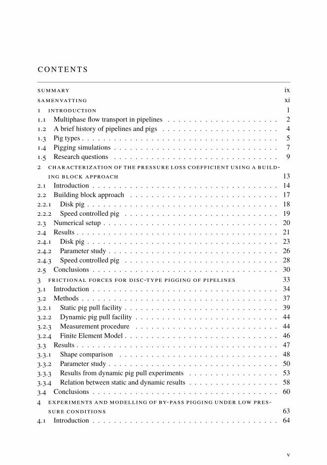
CONTENTS
summary ixsamenvatting xi1 introduction 11.1 Multiphase flow transport in pipelines . . . . . . . . . . . . . . . . . . . . . 21.2 A brief history of pipelines and pigs . . . . . . . . . . . . . . . . . . . . . . 41.3 Pig types . . . . . . . . . . . . . . . . . . . . . . . . . . . . . . . . . . . . . 51.4 Pigging simulations . . . . . . . . . . . . . . . . . . . . . . . . . . . . . . . 71.5 Research questions . . . . . . . . . . . . . . . . . . . . . . . . . . . . . . . 92 characterization of the pressure loss coefficient using a build-
ing block approach 132.1 Introduction . . . . . . . . . . . . . . . . . . . . . . . . . . . . . . . . . . . 142.2 Building block approach . . . . . . . . . . . . . . . . . . . . . . . . . . . . 172.2.1 Disk pig . . . . . . . . . . . . . . . . . . . . . . . . . . . . . . . . . . . . 182.2.2 Speed controlled pig . . . . . . . . . . . . . . . . . . . . . . . . . . . . . 192.3 Numerical setup . . . . . . . . . . . . . . . . . . . . . . . . . . . . . . . . . 202.4 Results . . . . . . . . . . . . . . . . . . . . . . . . . . . . . . . . . . . . . . 212.4.1 Disk pig . . . . . . . . . . . . . . . . . . . . . . . . . . . . . . . . . . . . 232.4.2 Parameter study . . . . . . . . . . . . . . . . . . . . . . . . . . . . . . . . 262.4.3 Speed controlled pig . . . . . . . . . . . . . . . . . . . . . . . . . . . . . 282.5 Conclusions . . . . . . . . . . . . . . . . . . . . . . . . . . . . . . . . . . . 303 frictional forces for disc-type pigging of pipelines 333.1 Introduction . . . . . . . . . . . . . . . . . . . . . . . . . . . . . . . . . . . 343.2 Methods . . . . . . . . . . . . . . . . . . . . . . . . . . . . . . . . . . . . . 373.2.1 Static pig pull facility . . . . . . . . . . . . . . . . . . . . . . . . . . . . . 393.2.2 Dynamic pig pull facility . . . . . . . . . . . . . . . . . . . . . . . . . . . 443.2.3 Measurement procedure . . . . . . . . . . . . . . . . . . . . . . . . . . . 443.2.4 Finite Element Model . . . . . . . . . . . . . . . . . . . . . . . . . . . . . 463.3 Results . . . . . . . . . . . . . . . . . . . . . . . . . . . . . . . . . . . . . . 473.3.1 Shape comparison . . . . . . . . . . . . . . . . . . . . . . . . . . . . . . 483.3.2 Parameter study . . . . . . . . . . . . . . . . . . . . . . . . . . . . . . . . 503.3.3 Results from dynamic pig pull experiments . . . . . . . . . . . . . . . . . 533.3.4 Relation between static and dynamic results . . . . . . . . . . . . . . . . . 583.4 Conclusions . . . . . . . . . . . . . . . . . . . . . . . . . . . . . . . . . . . 604 experiments and modelling of by-pass pigging under low pres-
sure conditions 634.1 Introduction . . . . . . . . . . . . . . . . . . . . . . . . . . . . . . . . . . . 64
v
[ January 15, 2020 at 7:46 – classicthesis version 2.2 ]

vi contents
4.2 Models . . . . . . . . . . . . . . . . . . . . . . . . . . . . . . . . . . . . . 664.2.1 Simplified model . . . . . . . . . . . . . . . . . . . . . . . . . . . . . . . 684.2.2 Full numerical model . . . . . . . . . . . . . . . . . . . . . . . . . . . . . 714.3 Experimental setup . . . . . . . . . . . . . . . . . . . . . . . . . . . . . . . 724.4 Results . . . . . . . . . . . . . . . . . . . . . . . . . . . . . . . . . . . . . . 754.4.1 Overall behaviour . . . . . . . . . . . . . . . . . . . . . . . . . . . . . . . 764.4.2 Local behaviour . . . . . . . . . . . . . . . . . . . . . . . . . . . . . . . . 794.4.3 Control . . . . . . . . . . . . . . . . . . . . . . . . . . . . . . . . . . . . 834.5 Conclusions . . . . . . . . . . . . . . . . . . . . . . . . . . . . . . . . . . . 875 analysis of time integration methods for the compressible two-
fluid model 895.1 Introduction . . . . . . . . . . . . . . . . . . . . . . . . . . . . . . . . . . . 905.2 Governing equations and characteristics . . . . . . . . . . . . . . . . . . . . 915.2.1 Compressible two-fluid model . . . . . . . . . . . . . . . . . . . . . . . . 915.2.2 Characteristics . . . . . . . . . . . . . . . . . . . . . . . . . . . . . . . . 925.2.3 Stability . . . . . . . . . . . . . . . . . . . . . . . . . . . . . . . . . . . . 935.2.4 Flow pattern map . . . . . . . . . . . . . . . . . . . . . . . . . . . . . . . 945.3 Spatial and temporal discretization . . . . . . . . . . . . . . . . . . . . . . . 965.3.1 Finite volume method on a staggered grid . . . . . . . . . . . . . . . . . . 965.3.2 Temporal discretization . . . . . . . . . . . . . . . . . . . . . . . . . . . . 985.4 Von Neumann analysis on the fully discrete equations . . . . . . . . . . . . . 995.4.1 Introduction . . . . . . . . . . . . . . . . . . . . . . . . . . . . . . . . . . 995.4.2 Extension to BDF2 and Crank-Nicolson . . . . . . . . . . . . . . . . . . . 1015.4.3 Amplification factor from simulation data . . . . . . . . . . . . . . . . . . 1025.5 Results for various test cases . . . . . . . . . . . . . . . . . . . . . . . . . . 1035.5.1 Kelvin-Helmholtz: linear wave growth . . . . . . . . . . . . . . . . . . . . 1045.5.2 Kelvin-Helmholtz: nonlinear wave growth . . . . . . . . . . . . . . . . . . 1075.6 Conclusions . . . . . . . . . . . . . . . . . . . . . . . . . . . . . . . . . . . 1116 modelling of by-pass pigging in two-phase stratified pipe flow 1136.1 Introduction . . . . . . . . . . . . . . . . . . . . . . . . . . . . . . . . . . . 1146.2 Numerical method . . . . . . . . . . . . . . . . . . . . . . . . . . . . . . . 1156.2.1 Spatial discretization . . . . . . . . . . . . . . . . . . . . . . . . . . . . . 1166.2.2 Regridding . . . . . . . . . . . . . . . . . . . . . . . . . . . . . . . . . . 1176.2.3 Boundary conditions . . . . . . . . . . . . . . . . . . . . . . . . . . . . . 1196.3 Pig motion . . . . . . . . . . . . . . . . . . . . . . . . . . . . . . . . . . . . 1226.3.1 A smooth function for the pig friction with the pipe wall . . . . . . . . . . 1236.4 Test cases . . . . . . . . . . . . . . . . . . . . . . . . . . . . . . . . . . . . 1256.4.1 Pig-generated slug for pigs without by-pass . . . . . . . . . . . . . . . . . 1256.4.2 Pig-generated slug for pigs with by-pass . . . . . . . . . . . . . . . . . . . 1286.5 Conclusions . . . . . . . . . . . . . . . . . . . . . . . . . . . . . . . . . . . 131
[ January 15, 2020 at 7:46 – classicthesis version 2.2 ]

contents vii
7 closure 1337.1 Conclusions . . . . . . . . . . . . . . . . . . . . . . . . . . . . . . . . . . . 1347.1.1 Pressure loss due to by-passing fluid . . . . . . . . . . . . . . . . . . . . . 1347.1.2 Friction between the pig and the pipe wall . . . . . . . . . . . . . . . . . . 1357.1.3 Lab-scale pigging experiments . . . . . . . . . . . . . . . . . . . . . . . . 1367.1.4 Numerical method for the 1D two-fluid model . . . . . . . . . . . . . . . . 1367.1.5 Pig simulation with the 1D two-fluid model . . . . . . . . . . . . . . . . . 1377.2 Recommendations for further research . . . . . . . . . . . . . . . . . . . . . 1377.2.1 Numerical simulations . . . . . . . . . . . . . . . . . . . . . . . . . . . . 1377.2.2 Lab experiments and field data . . . . . . . . . . . . . . . . . . . . . . . . 1387.2.3 Implementation of new results . . . . . . . . . . . . . . . . . . . . . . . . 139a two solution region 141b material tests 143c derivation of an analytic solution to the simplified model 147d two-fluid model details 149d.1 Geometry . . . . . . . . . . . . . . . . . . . . . . . . . . . . . . . . . . . . 149d.2 Friction models . . . . . . . . . . . . . . . . . . . . . . . . . . . . . . . . . 150
references 151acknowledgments 159curriculum vitæ 161list of publications 163
[ January 15, 2020 at 7:46 – classicthesis version 2.2 ]

[ January 15, 2020 at 7:46 – classicthesis version 2.2 ]

SUMMARY
The maintenance of pipelines for the production of oil or gas is usually done with a pig(Pipeline Inspection Gauge), which is a cylindrical device that just fits the pipe and prop-agates through the pipe along with the transport of fluids. While a conventional pig com-pletely seals the pipeline and travels with the same velocity as the production fluids, aby-pass pig has an opening which allows the fluids to partially by-pass the pig. The pur-pose of the present study is to get a better understanding of the physics of the pigging ofa pipeline with multiphase flow transport. The focus is on pigs with by-pass.
An important factor in determining the ultimate travel velocity of a by-pass pig is thepressure drop over the by-pass pig, which is characterized by a pressure loss coefficient.We investigate the pressure loss coefficient of three frequently used by-pass pig geome-tries in a single phase pipeline with Computational Fluid Dynamics (CFD). We present abuilding block approach for systematic modelling of the pressure loss through the by-passpigs, which takes the geometry and size of the by-pass opening into account. The CFDresults are used to validate the simple building block approach for systematic modellingof the pressure loss through a by-pass pig. It is shown that the models for the pressure lossclosely resemble the CFD results for each of the three pig geometries.In addition to the pressure loss coefficient, we investigate the frictional force which is
acting between the pig and the pipe wall. Two complementary experimental setups havebeen designed and used to study the sealing disc of a pig, which is responsible for thefrictional force between the pig and the pipe wall. Six 12′′ standard sealing discs fromtwo different vendors have been used. The first setup is a static setup in which the sealingdisc is subjected to a normal wall force and a tangential friction force. A unique featureof the setup is that the ratio between the friction force and the wall force can be readilyadjusted. This allows to experimentally determine the force ratio which is directly relatedto the Coulomb friction coefficient, which is often a difficult parameter to predict. Fur-thermore, the static setup is used to systematically study the effect of oversize, thickness,and Young’s modulus of the sealing disc on the frictional force. A direct comparison withFinite Element (FE) calculations is made. The second experimental facility consists of adynamic setup in which a sealing disc is pulled through a vertical 1.7 m long pipe. Theeffect of possible lubrication on the frictional force is studied by applying water to the slid-ing contact and comparing the results with dry pull tests for different sliding velocities.The corresponding difference in the Coulomb friction coefficient was quantified usingFE calculations, which were successfully verified with the static setup. The sensitivity ofpossible wear of the sealing disc on the frictional force was also considered.Furthermore, we have obtained experimental and numerical results for by-pass pigging
under low-pressure conditions. These are meant to help the design of a speed-controlled
ix
[ January 15, 2020 at 7:46 – classicthesis version 2.2 ]

x contents
pig; this is a pig in which the by-pass area is controlled during its propagation to maintaina desired velocity. Our study was carried out using air as working fluid at atmosphericpressure in a 52 mm diameter pipe with a length of 62 m. The experimental results havebeen used to validate simplified 1D models commonly used in the oil and gas industry tomodel transient pig behaviour. Due to the low-pressure conditions oscillatory behaviouris observed in the pig speed, which results in high pig velocity excursions. The oscillatorymotion is described with a simplified model which is used to design a simple controlleraimed at minimizing these oscillations. The controller relies on dynamically adjustingthe by-pass area, which allows to release part of the excess pressure which builds up inthe gas pocket upstream of the pig when the motion of the pig is arrested. Subsequently,the control algorithm is tested by a 1D transient numerical model, which was shown tosuccessfully reduce the pig velocity excursions.
In order to accurately solve the time dependent 1D two-fluid equations for multiphaseflow in pipelines, either with or without a pig, different time integration schemes havebeen investigated. The BDF2 method (Backward Differentiation Formula using 2 levels)is proposed as the preferred method to simulate transient compressible multiphase flow inpipelines. Compared to the prevailing Backward Euler method, the BDF2 scheme has asignificantly better accuracy (second order) while retaining the important property of un-conditional linear stability (A-stability). In addition, it is capable of damping unresolvedfrequencies such as acoustic waves present in the compressible model (L-stability), op-posite to the commonly used Crank–Nicolson method. A method for performing an au-tomatic von Neumann stability analysis is proposed that obtains the growth rate of thediscretization methods without requiring symbolic manipulations and that can be appliedwithout detailed knowledge of the source code. The strong performance of BDF2 is il-lustrated via several test cases related to the Kelvin–Helmholtz instability. A novel con-cept called Discrete Flow Pattern Map (DFPM) is introduced, which describes the effec-tive well-posed unstable flow regime as determined by the discretization method. BDF2accurately identifies the stability boundary, and reveals that in the nonlinear regime ill-posedness can occur when starting from well-posed unstable solutions. The well-posedunstable regime obtained in nonlinear simulations is therefore in practice much smallerthan the theoretical one, which might severely limit the application of the two-fluid modelfor simulating the transition from stratified flow to slug flow.The 1D code has been subsequently extended to model the propagation of a by-pass
pig in a two-phase pipeline. The liquid slug that is accumulated in front of the pig, theso-called pig-generated slug, has been modelled and characterized. Under the assumptionof a stratified flow, the academic case of liquid slug accumulation where we neglect theviscosity of the fluids has been analyzed. We also consider the more realistic case thatincludes the viscosity of the fluid. Finally, the effect of the presence of a by-pass in thepig on the accumulated liquid slug is investigated and compared to a simplified model.
[ January 15, 2020 at 7:46 – classicthesis version 2.2 ]

SAMENVATT ING
Voor het onderhoud van pijpleidingen in de olie- en gasindustie wordt normaliter gebruikgemaakt van een pig (pipeline inspection gauge), een cilindrisch instrument dat exact inde pijpleiding past en door de pijpleiding heen gaat samen met de productie van gas en/ofvloeistoffen. In tegenstelling tot de conventionele pig – die de pijpleiding compleet afsluiten voortbeweegt met dezelfde snelheid als de geproduceerde gas/vloeistoffen – heeft eenby-pass pig een opening die het mogelijk maakt om een deel van het gas of de vloeistofdoor de by-pass heen te laten stromen. Het doel van het huidige onderzoek is om een beterinzicht te krijgen in de fysica van het piggen van een pijpleiding in een meerfasenstroming,waarbij de nadruk van het onderzoek ligt op pigs met een by-pass.
Een belangrijke factor voor het bepalen van de uiteindelijke voortbewegingssnelheidvan de by-pass pig is de drukval over de by-pass pig, die gekarakteriseerd wordt doorde drukvalcoëfficiënt. We onderzoeken de drukvalcoëfficiënt voor drie veelgebruikte by-pass geometrieën in een één-fasepijpleiding door gebruik te maken van ComputationalFluid Dynamics (CFD). We presenteren een modulair opgebouwd systematisch modelvan de drukval over de by-pass pig, dat rekening houdt met de geometrie en afmetingvan de opening van de by-pass. De CFD-resultaten worden gebruikt om de eenvoudige,modulaire aanpak voor het systematisch modelleren van de drukval over de by-pass pigte valideren. Er wordt aangetoond dat de modellen voor de drukval goed overeenkomenmet de CFD-resultaten van elk van de drie by-passgeometrieën.Naast de drukvalcoëfficiënt doen we ook onderzoek naar de wrijvingskracht tussen de
pig en de pijpwand. Hiervoor zijn twee complementaire experimentele opstellingen ont-worpen om de afsluitschijf van de pig, die verantwoordelijk is voor de wrijvingskrachttussen de pig en de pijpwand, te bestuderen. Hierbij is gebruik gemaakt van een zestalstandaard 12′′ afsluitschijven, afkomstig van twee verschillende leveranciers. De eersteexperimentele opstelling is een statische opstelling, waarbij de afsluitschijf van de pigis onderworpen aan een normale wandkracht en een tangentiële wrijvingskracht. Eenuniek kenmerk van deze opstelling is de mogelijkheid om de verhouding tussen de wrijv-ingskracht en de wandkracht eenvoudig bij te stellen. Dit maakt het mogelijk om exper-imenteel de krachtenverhouding te bepalen welke direct gerelateerd is aan de Coulombwrijvingscoëfficiënt – een parameter die normaliter lastig te voorspellen is. Verder wordtde statische opstelling gebruikt om op systematische wijze het effect van de overmaat,dikte en Young’s modulus van de afsluitschijf op de wrijvingskracht te bestuderen. Hierbijwordt een directe vergelijking met eindige elementen berekeningen gemaakt. De tweedeexperimentele opstelling is een dynamische opstelling, waarbij de afsluitschijf door eenpijpleiding (met een lengte van 1.7 m) wordt getrokken. Het effect van mogelijke smeringop de wrijvingskracht is bestudeerd door water aan te brengen op het schuivende contact
xi
[ January 15, 2020 at 7:46 – classicthesis version 2.2 ]

xii contents
en door de testresultaten te vergelijken met de droge trekproef voor verschillende treksnel-heden. Het gevonden verschil in de Coulombwrijving is gekwantificeerd door gebruik temaken van de eindige elementen berekeningen, die succesvol waren geverifieerd door destatische opstelling. Hierbij is de gevoeligheid van mogelijke slijtage van de afsluitschijfop de wrijvingskracht ook in beschouwing genomen.
Verder hebben we experimentele en numerieke resultaten voor by-pass pigging on-der lagedrukcondities verkregen. Deze resultaten zijn bedoeld om te helpen bij het ont-werp van een pig met snelheidsregeling; dit is een pig waarbij de opening van de by-passgeregeld wordt gedurende de voortbeweging door de pijpleiding om een gewenste snel-heid te blijven houden. De studie is uitgevoerd met lucht op atmosferische druk in eenpijpleiding met een diameter van 52 mm en een lengte van 62 m. De experimentele resul-taten zijn gebruikt voor het valideren van vereenvoudigde 1D-modellen die typisch in deolie- en gasindustrie gebruikt worden. Door de lagedrukcondities wordt een oscillerendgedrag van de pigsnelheid waargenomen, wat resulteert in uitschieters in pigsnelheid. Deoscillerende beweging is beschreven door middel van een vereenvoudigd model dat ge-bruik maakt van een simpele regelaar gericht op het verminderen van deze oscillaties. Deregelaar zorgt voor de dynamische aanpassing van de by-passopening, waarbij een deelvan de opgebouwde overdruk in het gas aan de stroomopwaartse zijde van de pig kanworden vrijgelaten. Vervolgens is het regelalgoritme getoetst door middel van een tijd-safhankelijk 1D numeriek model, waarbij is aangetoond dat dit algoritme met succes deuitschieters in de pigsnelheid kan verminderen.Om de tijdsafhankelijke 1D vergelijkingen voor twee fluida bij meerfasenstroming in
pijpleidingen op te lossen, zowel met als zonder pig, zijn er verschillende tijdsintegrati-eschema’s onderzocht. De BDF2-methode (Backward Differentiation Formula, gebruik-makende van 2 niveaus) is voorgesteld als de voorkeursmethode om de dynamische com-pressibele meerfasenstroming in pijpleidingen te simuleren. In vergelijking met de gang-bare Backward-Euler methode heeft het BFD2-schema een aanzienlijk betere nauwkeurig-heid (tweede orde) terwijl dit schema het belangrijke kenmerk van onvoorwaardelijke lin-eaire stabiliteit (A-stabiliteit) behoudt. Ook is het schema, in tegenstelling tot de veelge-bruikte Cranck-Nicolson methode, in staat om onopgeloste frequenties, zoals geluidsgol-ven in het compressibele model (L-stabiliteit), te dempen. Een methode voor het uitvo-eren van een automatische von Neumann-stabiliteitsanalyse is voorgesteld, waarbij hetgroeipercentage van de discretisatiemethode wordt gevonden zonder dat symbolische ma-nipulaties zijn vereist. Deze methode kan worden toegepast zonder gedetailleerde kennisvan de broncode. De sterke prestatie van BFD2 is gedemonstreerd door middel van ver-schillende simulaties gerelateerd aan de Kelvin-Helmholtz instabiliteit. Een nieuw con-cept genaamd Discrete Flow Pattern Map (DFPM) is geïntroduceerd, dat het effectievegoedgestelde onstabiele stromingsregime beschrijft zoals bepaald door de discretisatieme-thode. BDF2 geeft een nauwkeurige bepaling van de stabiliteitsgrens en laat zien dat inhet niet-lineaire regime slechtgesteldheid kan optreden wanneer gestart wordt vanuit goed-gestelde onstabiele oplossingen. Het goedgestelde onstabiele regime in niet-lineaire simu-
[ January 15, 2020 at 7:46 – classicthesis version 2.2 ]

contents xiii
laties is om die reden in de praktijk velemalen kleiner dan het theoretische regime, hetgeende toepassing van het twee fluida model voor de simulatie van de gelaagde stroming naarzogenaamde "slug" stroming mogelijk ernstig beperkt.De 1D code is vervolgens uitgebreid om de voortbeweging van een by-pass pig in een
tweefasenpijpleiding te modelleren. De vloeistof die zich ophoopt voor de pig, de zoge-noemde pig-gegenereerde slug, is gemodelleerd en gekarakteriseerd. Met de aannamevan een gelaagde stroming is de academische casus geanalyseerd van de vloeistofophop-ing onder verwaarlozing van wrijving. We hebben ook de meer realistische casus, dierekening houdt met wrijving, in beschouwing genomen. Tenslotte is het effect van de aan-wezigheid van een by-pass in de pig op de vloeistofophoping onderzocht en vergelekenmet een vereenvoudigd model.
[ January 15, 2020 at 7:46 – classicthesis version 2.2 ]

[ January 15, 2020 at 7:46 – classicthesis version 2.2 ]

1I NTRODUCT ION
[ January 15, 2020 at 7:46 – classicthesis version 2.2 ]

2 introduction
chap
ter
1
1.1 multiphase flow transport in pipelines
Onshore or offshore pipelines provide an economic solution to the transport of fluids in theoil and gas industry. Offshore pipelines can transport the fluids from the reservoir and wellto an offshore production platform or to an onshore separator or slug catcher. Particularlygas-condensate pipelines (or trunklines) can have a large diameter (typically 30′′ to 42′′)and they can be long, with existing examples between 100 and 200 km [15]. Dependingon the gas production rate, significant amounts of condensate and water can accumulatein the pipeline (so-called liquid holdup). Therefore, the flow through these pipelines istypically characterized as multiphase flow. This means that gas, oil (or condensate), andwater (possibly accompanied by solids) are transported simultaneously through the samepipeline.Pipelines need regular maintenance. This is often by the use of so-called pigs. A pig (the
term is sometimes seen as an abbreviation for Pipeline Inspection Gauge) is a device thatis launched at the inlet of the pipeline and is received back in the pig trap, located at theoutlet of the pipeline. The pig is propelled by the production fluids that are transportedin the pipe. The pig can serve multiple maintenance purposes, which include: cleaningthe inner pipe wall, removing liquids, distribution of corrosion inhibitor along the pipewall, and pipe wall inspection. Figure 1.1a shows a schematic of a pig inside a multiphasepipeline.
Figure 1.1: (a) Conventional pig. (b) By-pass pig. Adapted from [21].
During the time that the pig resides in the pipeline it collects liquid in front of it, seefigure 1.1. This gives the so-called pig-generated volume. When this liquid arrives at theoutlet of the pipeline (i.e. just before the pig is received back in the trap), the liquid surge
[ January 15, 2020 at 7:46 – classicthesis version 2.2 ]

chapter1
1.1 multiphase flow transport in pipelines 3
will be stored in the downstream slug catcher. This pig-generated volume is about equalto the liquid holdup in the pipeline (present at the moment that the pig is launched) minusthe product of the normal liquid outflow rate with the pig residence time. As the onshoregas plant requires an uninterrupted supply of gas, a storage unit is needed onshore (down-stream of the pipeline and upstream of the plant) to temporarily park the liquid slug. Anexample of such a slug catcher is given in figure 1.2. The slug catcher consists of an inletheader and splitter, which distribute the liquid over a number of bottles, whereas the gasleaves the bottles at the upstream end through vertical gas legs. Liquid is drained at thedownstream liquid header. When a liquid slug arrives, the gas is displaced from the bot-tles and replaced by liquid. This guarantees uninterrupted supply of gas to the plant. Thedesign of the slug catcher size needs to be such that the pig-generated slug can indeed bestored in the bottles. Therefore the size can easily become as large as 5000 m3. These slugcatchers can be costly (50 to 150 million dollars) and require a significant plot space.
Figure 1.2: Example of a slug catcher with 5000 m3 liquid storage volume. Adapted from [39].
In an effort to reduce the pig-generated volume, so-called by-pass pigs have been designed.Whereas a conventional pig completely seals the pipeline, a by-pass pig has holes in thepig body which allows the gas to flow through (i.e. by-pass) the pig body. Figure 1.1bshows a schematic of a by-pass pig. As a result of the by-pass, the travel velocity of theby-pass pig will be lower as compared to a conventional pig. The longer residence time ofthe by-pass pig results in more time to drain the liquid slug from the slug catcher, whichwill in turn result in a smaller pig-generated volume that needs to be stored in the slugcatcher. In addition, the gas which flows through the by-pass pig drags the liquid in front
[ January 15, 2020 at 7:46 – classicthesis version 2.2 ]

4 introduction
chap
ter
1
of the pig, which results in a more elongated liquid slug and thus a smaller pig-generatedvolume, see figure 1.1b. In the most optimum situation the by-pass area is such large thatthe pig velocity is equal to the liquid velocity. In that case the pig-generated volume willbe reduced to zero. The typical size of the by-pass area ranges up to about 15% of the totalcross-sectional area of the pipe.
1.2 a brief history of pipelines and pigs
Pipes have been in use over many centuries. The Eqyptians used clay pipes for drainagepurposes as early as 4000 B.C. [56]. The Romans used lead and ceramic pipelines in theirfamous aqueducts more than 2000 years ago. The use of iron pipelines dates back to the18th century, which were used to transport water and gas. The subsequent advent of steelpipes in the 19th century allowed for much longer pipelines, as the steel could sustainmuch higher pressures than the iron pipelines. The discovery of oil in Pennsylvania in1859 was followed by the construction of the first long-distance steel pipeline in 1879.The pipeline had a diameter of 6′′ and a length of 109 miles. A major improvement inthe construction of steel pipelines occurred in the late 1920s with the introduction ofelectric arc welding, which allowed for leakproof connections of (large) pipe diametersegments [56]. The pipeline network has since then expanded rapidly in the U.S. andcounts a total of 2.23million kilometer in length and is thereby the most extensive pipelinenetwork of any country in the world [1]. The Netherlands has a total length around 20thousand kilometer of pipelines [1].An inevitable consequence of the operation of pipelines that transport large amounts
of fluids is appropriate internal maintenance. This was noted shortly after the first oilpipelines were taken into service in the 1870s. Higher pumping pressures and decreasedoverall efficiency reflected internal flow restriction due to build-up of wax and other debrisin the line [17]. The first pigs, which consisted of nothing more than a bundle of rags tiedtogether, were then used and resulted in immediate flow improvement. Later the rags werereplaced by bundles of leather which were stronger and could absorb the fluids and therebyswell, which guaranteed a good seal between the pig and the inner pipe wall. Later onpigs were more purposefully built, consisting of a steel body with urethane cups or discs,possibly equipped with brushes and scrapers. In the 1960s the polyurethane foam pigwas introduced. Many other industries also adapted the use of foam pigs, including thewater and processing industry. From the late 1960s onwards pigs became instrumentedwith various sensors which can inspect the condition of the inner pipe wall while the pigis travelling through the pipe [17]. These developments have lead to so-called smart (orintelligent) pigs.It is unclear where the term ’pig’ is originating from. As mentioned some people refer
to pig as an abbreviation of Pipeline Inspection Gauge [15]. But as pigs were initially notused for inspection purposes, this is unlikely. A more accepted explanation is that the term
[ January 15, 2020 at 7:46 – classicthesis version 2.2 ]

chapter1
1.3 pig types 5
pig is attributed to the screeching sound that the pig can make when it moves inside thepipeline [15, 17, 74].
1.3 pig types
Pigs were originally developed to remove deposits which could obstruct or retard the flowthrough a pipeline. Today pigs are widely used during all phases in the life of a pipelinefor many different reasons in various industries, including water, oil, food, and chemi-cals. While there are more than 350 different pig types [15], three main categories can bedistinguished:
• Cleaning/maintenance pigs.These are used to clean the pipeline to ensure continu-ous flow andmaintain operational efficiency or to prepare the pipeline for intelligentinspection.
• Intelligent inspection tools. These are used to inspect the pipeline, to provide in-formation on the condition of the line and to assess the extent and location of anyintegrity concerns.
• Gel pigs. These are pumpable liquid gels sealed between two cleaning/maintenancepigs to remove the solid debris or water from the pipeline.
A pig that enters a pipeline is driven forward by the higher pressure of the fluid behind it,which pushes the pig from one end to the other end of the pipeline. During its residencein the pipeline, the pig sweeps out the entire content of the pipeline. Some of the reasonsto send a pig through a pipeline are:
• Corrosion management. To reduce the corrosion rate of the pipeline, a pig canremove corrosion products, stagnant water, and corrosion causing microbes in thelow spots. Pigging can also help to more uniformly distribute the corrosion inhibitorthroughout the pipeline, such as to enable wetting of the top pipewall with corrosioninhibitor in the liquid. When using a by-pass pig for corrosion distribution in wetgas pipelines, one needs tomake sure that the flow regime ahead of the pig still givestop-of-line wetting; this is ensured by the liquid slug created ahead of the pig if astandard pig is used (no by-pass), but this will depend on the rate of the by-passinggas flow if a by-pass pig is used.
• Removal of solids. These solids can be for example wax or scale sticking to theinside of the pipeline or sand or corrosion products that have accumulated in thepipeline.
• Removal of liquids. The build-up of liquid in a pipeline to reach the steady-state liq-uid hold-up can take days or weeks. By pigging at regular intervals, and thus through
[ January 15, 2020 at 7:46 – classicthesis version 2.2 ]

6 introduction
chap
ter
1
regular liquid removal, one can keep the liquid hold-up below the steady-state equi-librium liquid hold-up, for example to ensure that the liquids in the pipeline canalways fit within the slug catcher.
• Pipeline inspection to determine the integrity. A pig equipped with special mea-suring equipment like ultrasonic transducers or Magnetic Flux Leakage (MFL)can determine the integrity of the pipeline by measuring the remaining wall thick-ness [27].
In a multiphase flow pipeline, gas travels on average faster than liquid. A conventionalpig (i.e. a pig without by-pass) travels at the mixture velocity through the pipeline, as nofluid can by-pass the pig. This mixture velocity is in between the gas and liquid velocity. Aconventional pig travels thus faster than the liquid. The pig will collect the liquid in front ofit as it moves faster than the liquid velocity, see figure 1.1. Behind the pig, there will onlybe gas present, as liquid is travelling slower than the pig and the liquid is staying behindto re-establish the steady-state liquid hold-up in the pipeline. As explained in section 1.1,a by-pass pig travels at a lower velocity compared to a conventional pig. The by-passarea can be created in various ways. Figure 1.3 shows two examples of a by-pass pig. Thefirst example (figure 1.3a) shows a by-pass pig with a concentric by-pass area in the centre,whereas in the second example (figure 1.3b) a deflector plate is included at the downstreamside of the by-pass. The small space between the pig body and the plate creates the by-pass.The main function of the deflector plate is providing a pulling force, which is especiallyneeded when the pig is launched [96].
Figure 1.3: (a) By-pass pig with by-pass in the centre (taken from [53]). (b) By-pass pig with adeflector disc (taken from [96]).
Many other by-pass configurations do exist. The advantage of using a by-pass pig com-pared to a conventional pig is not only the reduction of the pig-generated volume (asexplained in section 1.1). Also for the removal of solids, which may be attached to thewall in liquid pipelines, the use of a by-pass pig can be beneficial: due to the flow throughthe by-pass liquid jets can emerge, which help to remove the solids from the wall andtransport them as a slurry further downstream. The lower travel speed of a by-pass pig isalso beneficial for intelligent pigs. The inspection of the pipe wall, which is carried out
[ January 15, 2020 at 7:46 – classicthesis version 2.2 ]

chapter1
1.4 pigging simulations 7
by the intelligent pig, is much more accurate at a lower travel speed, and may even beimpossible in case no by-pass is present and the pig travels at the mixture velocity. Forexample, a high velocity of the inspection pig can cause low pipe wall thickness locationsto be missed.Although the advantages of using a by-pass pig are clear, the use of a by-pass pig
does not come without any risks. The most important risk is that, due to the by-passarea, not enough differential pressure across the pig is generated and the pig gets stuckin the pipeline. The costs associated with locating and removing a stuck pig in combi-nation with the production deferment caused by such an event are high. This makes thechoice of the by-pass area, which needs to be made upfront of carrying out the piggingrun, a challenging task. The main uncertainty for calculating the right by-pass openingis the friction between the pig and the pipe wall. To overcome this problem, inspectionpigs have been designed that have an adjustable by-pass area to regulate the pig speedthrough the pipeline to a constant velocity [63, 89]. These so-called speed-controlled pigshave an onboard controller, which reacts on the changes in the friction between the pigand the pipe wall along the pipeline, as this leads to a change in the pig velocity. Forexample, a local increase in friction could cause the pig to slow down. The by-pass open-ing is then reduced by the control algorithm and as a result the pressure drop across thepig increases and therefore the pig velocity increases as well. Speed-controlled pigs havenormally been applied in single-phase pipelines, but there are also some first field appli-cations to use them under multiphase flow conditions. So far speed-controlled by-passpigging has been mainly found on intelligent pigs in order to improve inspection quality.But there is a potential to apply similar technology to other pig types as well.
1.4 pigging simulations
As explained in the previous section, it is important to have a proper design of the piggingoperation before carrying out the actual pigging run. Some typical questions that couldbe addressed during such a design phase are:
• What will be the additional pressure drop in the pipeline as a result of the presenceof a pig?
• What will be the size of the pig-generated liquid slug, and at what time will it arriveat the slug catcher?
• What is the optimal size of the by-pass area?
• At what travel speed will the pig traverse the pipeline?
In almost all cases the most important question is: Will the pig arrive at the outlet of thepipe at all? In an attempt to answer these questions the industry uses various simplifiedmodels. We will outline a few of the existing modelling approaches below.
[ January 15, 2020 at 7:46 – classicthesis version 2.2 ]

8 introduction
chap
ter
1
In order to estimate the friction of the pig with the pipe wall (or equivalently: the drivingdifferential pressure that is needed to overcome the frictional force), the following empir-ical relationship has been proposed by Cordell [14]: ∆Ppig(bar) = K
Dnom(in) . Here∆Ppig is the required differential pressure (in bar unit) needed to drive the pig,Dnom isthe nominal pipeline diameter (in inch unit), and K is an empirical constant. Figure 1.4 de-picts different K-values for different pig types. For example: a value of K = 1 correspondsto a foam pig, a value of K = 19 corresponds to an ultrasonic technique in line inspectiontool, whereas K = 24 would correspond to a magnetic flux leakage (MFL) in line inspec-tion tool. It is clear that the K-values are indicative only. Many pigs have a sealing discthat guarantees a tight seal between the pig and the inner pipe wall, see figure 1.3b. It isthis sealing disc that is responsible for the frictional force. No information on the materialproperties nor on the size of the sealing disc is present in the aforementioned model.
Figure 1.4: Proportionality factor to calculate the differential pressure that is required to drivevarious types of pigs. Adapted from [14].
In many cases the precise value of the friction is not very important for conventionalpigs (i.e. no by-pass) as usually the pressure drop across the pig (a few bar maximum) ismuch smaller than the total pressure drop along the pipeline. However, when a by-passpig is used it is an important factor, as the pressure drop that is generated as a result ofthe by-passing fluids must overcome the frictional force. When the by-pass is too largenot enough pressure drop is generated, and the pig stalls. It is this balance between thedriving pressure force and the frictional force that ultimately determines the travel velocityof a by-pass pig. Not many models exist for predicting the pressure drop due to the by-passing fluids across a by-pass pig, and often a simple geometry, like the one presented infigure 1.3a, is assumed [68, 82].
[ January 15, 2020 at 7:46 – classicthesis version 2.2 ]
chapter1
1.5 research questions 9
In order to model the pig trajectory through the pipe, the industry frequently uses one-dimensional transient pipelinemodels to simulate themultiphase flowwith the pigging op-eration. Two examples of commercial simulation tools are OLGA [8] and LedaFlow [28].These tools solve the conservation equations for mass, momentum, and energy for each ofthe phases. The equations have been averaged over the cross-sectional area of the pipeline,which means that the 3D spatial equations are converted into 1D spatial equations. Theaveraging leads to closure relations for the wall friction and for the interfacial stress be-tween the phases. The 1Dmodels also include empirical correlations for the different mul-tiphase flow regimes (e.g. stratified flow, hydrodynamic slug flow, bubbly flow, or annulardispersed flow). The pipeline is split up in a number of spatial grid cells, and a numericaltime step has to be chosen. The propagation of the pig can also be simulated with these1D tools. User input is required for the friction between the pig and the pipe wall (both forconventional pigs and for by-pass pigs) and for the pressure loss due to by-passing fluid(for the case with by-pass pigs). The precise details on how the conservation equations arenumerically solved, as well as how the fluid-pig interaction is handled, are proprietary tothe vendors of these commercial tools. Academic codes do exist, but are often limited tosingle-phase flow. Only a few consider two-phase flow [47, 50, 61, 97], but among thoseonly a pig without by-pass is considered.
1.5 research questions
The purpose of the present PhD project is to get a better fundamental understanding ofthe physics of pigging of a pipeline with multiphase flow transport in order to improveengineering models used in the industry for pigging operations. Although pigs have beenused for decades in the industry, by-pass pigs are relatively new, and the use of pigs withspeed control has emerged just recently. As explained, many empirical relations exist butsome fundamental knowledge about the physics is lacking. The emphasis in our researchwill be on by-pass pigs, either without or with speed control. The results can be usedfor implementation in the engineering design tools that are used to prepare a piggingoperation. In this way a better design can be made for by-pass pigs, either without orwith speed control. This reduces the risk that something will go wrong with the actualoperation of the pig, such as serious oscillations in the pig movement or a stalled pig. Incase of speed-controlled by-pass pigs this will also help to determine the range of the by-pass opening that should be available for control. The reduced, or eliminated, operationalrisks of by-pass pigging will help to safely reduce the size of the required slug catcher thatwould be required for conventional pigging.
The focus will be on various aspects which are important for the motion of a by-passpig in a single phase or multiphase pipeline:
1. Fluid flow aspects. The flow will be calculated with both a 1D approach, using anewly developed numerical-physical model, and with 2D and 3D Computational
[ January 15, 2020 at 7:46 – classicthesis version 2.2 ]

10 introduction
chap
ter
1
Fluid Dynamics (using the existing third-party tool Fluent). Lab experiments werecarried out in the water/air flow loop at the Delft University of Technology.
2. Friction between the pig and the pipe wall. Finite element simulations were car-ried out for the deformation of the oversized discs that are part of the by-pass pigconfiguration. Also pull tests with such discs were carried out in a newly built set-upat the Shell Technology Centre Amsterdam (STCA).
3. Control of the by-pass opening to obtain the desired pig velocity. Some small-scale tests with pigs were carried out in the water/air flow loop at the Delft Univer-sity of Technology. In parallel simulations were carried out with the 1D model.
The results of the study are described in 5 technical chapters. These chapters are based onpublications that appeared either in conference proceedings or in journals.
Chapter 2. CFD simulations with Fluent to obtain the pressure loss coefficient for theby-pass fluid through the by-pass area. The effect of different by-pass configurations isstudied in singple phase flow. The work was carried with the support of two Master stu-dents [4, 54], and theworkwas presented at a conference and published in a journal [5, 35].
Chapter 3. Experiments and modelling for the friction between the pig and the wall. Thework was carried out with the support from two Master students [29, 32]. This includedexperiments at STCA (both steady state and dynamic pull tests, with dry gas, and withlubrication using water and air). The forces and disc deformation as measured were com-pared with Finite Element simulations for the stresses and deformations. The results werepresented at a conference and published in a journal [34, 58].
Chapter 4. Lab experiments in water/air 2”, 130 m flow loop at the Delft University ofTechnology. The work was carried out with the support from a Master student [44] andfrom a team of 4 undergraduate students. The pressure drop over the pig and its velocitywere measured using air only at atmospheric pressure. Various configurations (withoutand with by-pass) were measured, and the observed slip-stick behaviour (that is typicalfor low pressure pigging) was reproduced with a simple analytical model. The results werepresented at a conference and published in a journal [36, 37].
Chapter 5. Numerical modelling of two-phase pipe flow (still without the presence ofa pig). An accurate spatial and temporal finite volume scheme to solve the 1D two-fluidmodel was developed and tested in Matlab. Simulations were carried out for the stabilityof stratified gas-liquid flow. The growth of roll waves and slugs was simulated. A numer-ical flow pattern map could be established. Part of the results have been published in ajournal [80].
[ January 15, 2020 at 7:46 – classicthesis version 2.2 ]

chapter1
1.5 research questions 11
Chapter 6. Numerical modelling of pigs with the help of an accurate two-fluid model.Thereto the newly developed finite volume code was extended with the propagation ofpigs. The results from the other parts of the study (such as the pressure loss coefficientdetermined with CFD for the by-passing fluid, and the friction between the pig and thepipe wall) were used as input correlations to the pigging model in the 1D numerical model.The results have been published at a conference [38].
[ January 15, 2020 at 7:46 – classicthesis version 2.2 ]

[ January 15, 2020 at 7:46 – classicthesis version 2.2 ]

chapter2
2CHARACTER IZAT ION OF THE PRESSURE LOSSCOEFF IC I ENT US ING A BU ILD ING BLOCK APPROACH
This chapter is adopted from M. H. W. Hendrix, X. Liang, W.-P. Breugem, and R. A. W. M. Henkes, "Char-acterization of the pressure loss coefficient using a building block approach with application to by-pass pigs".In: Journal of Petroleum Science and Engineering 150 (2017), pp. 13-21.
13
[ January 15, 2020 at 7:46 – classicthesis version 2.2 ]
14 characterization of the pressure loss coefficient using a building block approach
chap
ter
2
2.1 introduction
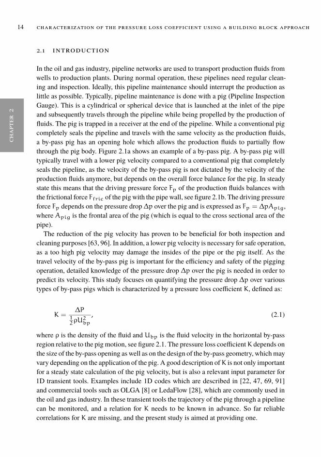
In the oil and gas industry, pipeline networks are used to transport production fluids fromwells to production plants. During normal operation, these pipelines need regular clean-ing and inspection. Ideally, this pipeline maintenance should interrupt the production aslittle as possible. Typically, pipeline maintenance is done with a pig (Pipeline InspectionGauge). This is a cylindrical or spherical device that is launched at the inlet of the pipeand subsequently travels through the pipeline while being propelled by the production offluids. The pig is trapped in a receiver at the end of the pipeline. While a conventional pigcompletely seals the pipeline and travels with the same velocity as the production fluids,a by-pass pig has an opening hole which allows the production fluids to partially flowthrough the pig body. Figure 2.1a shows an example of a by-pass pig. A by-pass pig willtypically travel with a lower pig velocity compared to a conventional pig that completelyseals the pipeline, as the velocity of the by-pass pig is not dictated by the velocity of theproduction fluids anymore, but depends on the overall force balance for the pig. In steadystate this means that the driving pressure force Fp of the production fluids balances withthe frictional force Ffric of the pig with the pipe wall, see figure 2.1b. The driving pressureforce Fp depends on the pressure drop∆p over the pig and is expressed as Fp = ∆pApig,where Apig is the frontal area of the pig (which is equal to the cross sectional area of thepipe).The reduction of the pig velocity has proven to be beneficial for both inspection and
cleaning purposes [63, 96]. In addition, a lower pig velocity is necessary for safe operation,as a too high pig velocity may damage the insides of the pipe or the pig itself. As thetravel velocity of the by-pass pig is important for the efficiency and safety of the piggingoperation, detailed knowledge of the pressure drop ∆p over the pig is needed in order topredict its velocity. This study focuses on quantifying the pressure drop ∆p over varioustypes of by-pass pigs which is characterized by a pressure loss coefficient K, defined as:
K =∆P
12ρU
2bp
, (2.1)
where ρ is the density of the fluid and Ubp is the fluid velocity in the horizontal by-passregion relative to the pig motion, see figure 2.1. The pressure loss coefficientK depends onthe size of the by-pass opening as well as on the design of the by-pass geometry, whichmayvary depending on the application of the pig. A good description ofK is not only importantfor a steady state calculation of the pig velocity, but is also a relevant input parameter for1D transient tools. Examples include 1D codes which are described in [22, 47, 69, 91]and commercial tools such as OLGA [8] or LedaFlow [28], which are commonly used inthe oil and gas industry. In these transient tools the trajectory of the pig through a pipelinecan be monitored, and a relation for K needs to be known in advance. So far reliablecorrelations for K are missing, and the present study is aimed at providing one.
[ January 15, 2020 at 7:46 – classicthesis version 2.2 ]

chapter2
2.1 introduction 15
Figure 2.1: (a) A bi-directional by-pass pig, taken from [53]. (b) A schematic of the forces on aby-pass pig in a horizontal pipeline. In steady state the driving force Fp due to theby-passing fluids is balanced by the frictional force Ffric of the pig with the pipe wall.In this schematicD indicates the pipe diameter, d the diameter of the by-pass hole, Uthe upstream bulk velocity, and Upig the pig velocity.
[ January 15, 2020 at 7:46 – classicthesis version 2.2 ]

16 characterization of the pressure loss coefficient using a building block approach
chap
ter
2
Flow
Adjustable
by-pass valve
Figure 2.2: (a) A by-pass pig with a deflector disk, taken from [96]. (b) Schematic of a by-pass pigwith speed control. The by-pass valve can be adjusted to regulate the by-pass area.
As the geometry of a pig varies depending on its application, a building block approachis used in order to provide a general framework for determining the corresponding pressureloss coefficient. The building block approach relies on a geometrical decomposition ofthe by-pass pig, and accounts for the contribution of the individual components of the by-pass pig geometry to the overall pressure loss. It is thus assumed that the flow patterns areuncorrelated between building blocks, i.e. the local flow pattern within a building blockdepends solely on geometrical characteristics of that building block. In order to validatethe building block approach a CFD (Computational Fluid Dynamics) approach is appliedto model fully turbulent single phase flow through various types of by-pass pigs. The bulkReynolds number is fixed at Re = UD/ν = 107, where ν is the kinematic viscosity of thefluid, U is the average velocity, and D is the pipe diameter. A similar Reynolds numberhas been used in a previous CFD study on by-pass pigs [82], which allows for a directcomparison of the new results obtained in this work. From the CFD results the pressureloss coefficient K can be extracted.The building block approach is tested on three different by-pass pig geometries encoun-
tered in the industry. First the relatively simple design of the bi-directional by-pass pig isrevisited, which is shown in figure 2.1a. Furthermore, the by-pass pig shown in figure 2.2ais considered, which is referred to as the disk pig. This pig has a deflector plate, or disk,added at the exit of the by-pass pig. The deflector plate helps to get the pig into motionwhen the pressure drop over the pig is relatively small [96]. Finally, a by-pass pig designwhich is shown in figure 2.2b is considered. This by-pass pig has an adjustable by-passarea by making use of a rotatable valve. The angular position of the valve determines theopening of the by-pass holes. The adjustable by-pass enables control of the pressure dropover the pig and thus control of the speed of the pig. This by-pass pig is therefore referredto as the speed controlled pig. Examples of speed controlled pigs can be found in [63, 89].The structure of the paper is as follows. In section 2.2 a literature review is given on
theory and correlations for by-pass pig geometries and the building block approach is ex-plained. Section 2.3 describes the numerical setup which is used for the CFD calculations.
[ January 15, 2020 at 7:46 – classicthesis version 2.2 ]

chapter2
2.2 building block approach 17
Results obtained from the CFD simulations are discussed in section 2.4. A summary ofthe results and possibilities for future research are given in section 2.5.
2.2 building block approach
In previous research the pressure loss coefficient of a bi-directional by-pass pig, Kbidi,was studied using CFD [82]. It was found that Kbidi can be successfully described bythe Idelchik correlation for a thick orifice, as the bi-directional by-pass pig has a shapecomparable with a thick orifice, see figure 2.1. For sufficiently thick orifices (Lpigd > 3)the Idelchik correlation for a thick orifice reads [45]:
Kbidi = 0.5(1−
A0A1
)0.75
+4fLpig
d+
(1−
A0A1
)2, (2.2)
where A0 = 14πd
2 is the cross-sectional area of the by-pass and A1 = 14πD
2 is thecross-sectional area of the pipe. The length of the pig is denoted by Lpig and f is theFanning friction coefficient, which is determined by the Churchill relation [13] using theReynolds number defined in the horizontal by-pass area, that is f = f(Ubpd/ν). Here itis assumed that the walls of the by-pass area are hydrodynamically smooth, which impliesthat the friction factor is not a function of the wall roughness. This correlation for a thickorifice can be regarded as a linear combination of the loss associated with the inlet of thepig (contraction loss), the by-pass area of the pig (wall friction), and the outlet of the pig(expansion loss), see figure 2.3.
Figure 2.3: Break down of the pressure loss coefficient of a bi-directional by-pass pig in a roundpipe. Symbols are explained in the text.
The use of this ’building block’ approach to model the pressure loss coefficient of aby-pass pig has been suggested in previous work [67, 68], and was validated recently with
[ January 15, 2020 at 7:46 – classicthesis version 2.2 ]

18 characterization of the pressure loss coefficient using a building block approach
chap
ter
2
CFD for a bi-directional by-pass pig [5, 82]. In this study it is attempted to use this buildingblock approach for a more general class of by-pass pigs, namely the disk pig and the speedcontrolled pig, as depicted in figure 2.2. In order to model these more complex shapedpigs it is suggested to modify the last term of equation 2.4. This last term is associatedwith the pressure loss of a sudden expansion, which is also known as the Borda-Carnotequation. This equation holds very well for a fully turbulent flow [60, 87]. It is importantto note that the Borda-Carnot equation, along with the other contributions in equation 2.2,is associated with irreversible losses. It thus describes the change in total pressure Pt:
∆Pt =1
2ρU2bpKbidi (2.3)
As the pipe area is considered constant, the dynamic pressures upstream and downstreamof the pig are equal. Therefore, the static pressure drop ∆P over the pig can be consideredequal to the total pressure drop ∆Pt.The fact that for both the disk pig and the speed controlled pig the exit of the pig can no
longer be regarded as a sudden expansion emphasizes the need for a different correlationthan equation 2.2. A new correlation for the disk pig and the speed controlled pig is nowsuggested.
2.2.1 disk pig
In order to replace the last term in the original Idelchik correlation 2.2 the geometry of adisk valve depicted in figure 2.4a is considered first.
Figure 2.4: (a) Disk valve geometry, adopted from [45] (b) Schematic of the disk pig.
The geometry is taken from [45], in which the following correlation for the pressureloss coefficient of this geometry is proposed:
Kdv =2H
d+0.155d2
h2− 1.85. (2.4)
[ January 15, 2020 at 7:46 – classicthesis version 2.2 ]

chapter2
2.2 building block approach 19
This equation is reported to be valid within the range:
0.1 <h
d< 0.25, (2.5)
and
1.2 <H
d< 1.5. (2.6)
The validity of equation 2.4 outside this range has not been established. Kdv is associatedwith the velocity scale Ubp, see figure 2.4a. A schematic of the disk pig shown in fig-ure 2.2a is depicted in figure 2.4b. The outlet of the disk pig can be represented by a diskvalve as shown in figure 2.4a. The by-pass area of the disk pig Adv, which is defined bythe smallest by-pass area of the pig, is given by:
Adv = πdh. (2.7)
Replacing the last term of equation 2.2 with the loss coefficient of a disk valve, equa-tion 2.4, the following correlation for the pressure loss coefficient of a disk pig Kdp isproposed:
Kdp = 0.5(1−
A0A1
)0.75
+4fLpig
d+
(2H
d+0.155d2
h2− 1.85
). (2.8)
Note that the thickness of the disk t is not appearing in the proposed correlation. It isassumed that the flow is separating from the edge of the disk and will not reattach to thedisk. This implies that the thickness is sufficiently small to neglect its influence on theflow.
2.2.2 speed controlled pig
The speed controlled pig with a by-pass regulating valve as shown in figure 2.2b is mod-elled as a valve consisting of a disk with four adjustable opening slots, see figure 2.5a. Theangle ω defines the opening angle of the slots in degrees. In figure 2.5b a cross-sectionof the speed controlled pig is shown.
The smallest by-pass area of the speed controlled pig Asp is defined as:
Asp = πHihnω
360, (2.9)
[ January 15, 2020 at 7:46 – classicthesis version 2.2 ]
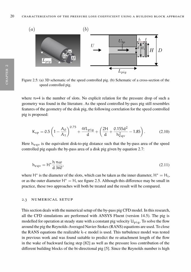
20 characterization of the pressure loss coefficient using a building block approach
chap
ter
2
Figure 2.5: (a) 3D schematic of the speed controlled pig. (b) Schematic of a cross-section of thespeed controlled pig.
where n=4 is the number of slots. No explicit relation for the pressure drop of such ageometry was found in the literature. As the speed controlled by-pass pig still resemblesfeatures of the geometry of the disk pig, the following correlation for the speed controlledpig is proposed:
Ksp = 0.5(1−
A0A1
)0.75
+4fLpig
d+
(2H
d+0.155d2
h2eqv− 1.85
). (2.10)
Here heqv is the equivalent disk-to-pig distance such that the by-pass area of the speedcontrolled pig equals the by-pass area of a disk pig given by equation 2.7:
heqv = H∗h
d
nω
360, (2.11)
whereH∗ is the diameter of the slots, which can be taken as the inner diameter,H∗ = Hi,or as the outer diameterH∗ = H, see figure 2.5. Although this difference may be small inpractice, these two approaches will both be treated and the result will be compared.
2.3 numerical setup
This section deals with the numerical setup of the by-pass pig CFDmodel. In this research,all the CFD simulations are performed with ANSYS Fluent (version 14.5). The pig ismodelled for operation at steady state with a constant pig velocityUpig. To solve the flowaround the pig the Reynolds-AveragedNavier-Stokes (RANS) equations are used. To closethe RANS equations the realizable k-ε model is used. This turbulence model was testedin previous work and was found suitable to predict the re-attachment length of the flowin the wake of backward facing step [82] as well as the pressure loss contribution of thedifferent building blocks of the bi-directional pig [5]. Since the Reynolds number is high
[ January 15, 2020 at 7:46 – classicthesis version 2.2 ]

chapter2
2.4 results 21
(Re = 107) in the CFD calculations, standard wall functions are applied for the near wallregion treatment. The effect of wall roughness is neglected. It is thus assumed that thewalls are hydrodynamically smooth.
OutletInlet
Figure 2.6: Numerical setup. The inlet is located at the left. The equations are solved in a refer-ence frame that moves with the pig. As a result, the pipe wall moves with a velocityUwall = −Upig.
Figure 2.6 shows a schematic of the numerical setup. The RANS equations are solvedin a moving reference frame of the pig [5, 82]. This means that the walls have a nonzerovelocity Uwall equal to Uwall = −Upig. A User Defined Function (UDF) is applied atthe inlet to prescribe a fully developed turbulent pipe flow profile. At the outlet a constantvalue for the static pressure is prescribed. In figure 2.7 the mesh that is used is shown. Astructured mesh for all the simulations is employed which is constructed by dividing thedomain in different sub-domains with a controlled number of nodes on each edge. Thisway the number and shape of the computational cells in each region can be controlled.Figure 2.7b shows the mesh in the cross-sectional plane indicated by the dashed blackline in figure 2.7a. An enlargement of the region within the white square in shown infigure 2.7c. The black arrow indicates a region of mesh refinement. The location of thismesh refinement corresponds to the radius of the horizontal by-pass area in order to refinethe grid near the wall of the by-pass area. The same procedure is applied to the mesh atthe inner pipe wall. The typical maximum value of y+ in the simulation is around 4500,which is well within the range 30 < y+ < 20000 for which the flow is in the logarithmiclayer, and standard wall function can be used to predict the velocity profile, see [24, 51].
2.4 results
In this section the CFD results for the disk pig are discussed first. The obtained values forthe pressure loss coefficientK are compared with the correlation suggested in equation 2.8.Next, the CFD results for the speed controlled pig are discussed. The obtained K valueswill be compared with equation 2.10. For the disk pig axi-symmetry is assumed and the
[ January 15, 2020 at 7:46 – classicthesis version 2.2 ]

22 characterization of the pressure loss coefficient using a building block approach
chap
ter
2
x/D (-)
0 0.1 0.2
y/D
(-)
0
0.1
0.2
x/D (-)
-0.4 -0.2 0 0.2 0.4
y/D
(-)
-0.4
-0.2
0
0.2
0.4
Figure 2.7: (a) Blocks that represent different regions in streamwise direction. (b) Details of themesh on the cross-sectional plane indicated by the dashed line in panel a. (c) Enlarge-ment of the area indicated by the white square.
[ January 15, 2020 at 7:46 – classicthesis version 2.2 ]

chapter2
2.4 results 23
CFD simulation is 2D, but for the speed controlled pig no axi-symmetry exists and theCFD simulation is 3D.
2.4.1 disk pig
The flow around a disk pig has already been studied by Korban et al. [5]. In their study,the relation between the pressure loss coefficient K and the parameters which govern thedisk pig model, was investigated. The K value of the disk pig was found to be around2 to 3 times higher than the typical value that is found for a bi-directional pig (withoutdisk). However, a general correlation to predict the pressure loss coefficient K for a diskpig was not given. Thus, in the present research, the flow around the disk pig is furtherinvestigated. Table 2.1 summarizes the key parameters which define a base case for thedisk pig simulations. These parameters are based on a realistic scenario, which can befound in [96]. The parameters will be varied through using the following dimensionlessnumbers which define the disk pig geometry:
• Horizontal by-pass area fraction: (d
D)2
• Dimensionless disk height:H
D
• Disk by-pass area fraction:4dh
D2
As discussed in section 2.2, the effect of the dimensionless disk thickness t/D as wellas the dimensionless pig length Lpig/D are not studied here.First of all, the flow features of the disk pig are presented. Interestingly, two different
types of flow behaviour around the disk pig have been observed in the simulation results.Secondly, various parameter studies are carried out, in order to study the relation betweenthe pressure loss coefficient K and the governing parameters of the disk pig model.
2.4.1.1 Flow features of disk pig
Figure 2.8 shows the streamlines that represent the mean flow around the disk pig. Thefluid enters the pig through a sudden contraction. The flow behaviour in this region is sim-ilar to that of the conventional bi-directional pig [5]. After the horizontal by-pass region,the flow moves around the disk. In the disk by-pass region, the flow expands radially out-ward and has a jet-like structure. The flow subsequently detaches from the disk creating arecirculation zone downstream of the pig. To give insight in the pressure loss for the disk
[ January 15, 2020 at 7:46 – classicthesis version 2.2 ]

24 characterization of the pressure loss coefficient using a building block approach
chap
ter
2
Table 2.1: Key parameters that govern the disk pig study.
Parameter ValueBulk velocity U 2.87m/sHorizontal by-pass area (%) 10%Disk by-pass area (%) 8%Pipe diameter D 1.16mBy-pass pig diameter d 0.3668mUpstream pipe length Lup 5DDownstream pipe length Ldown 20DPig length Lpig 2mPig velocity 2m/sDistance between the pig body and the disk h 0.06303DDisk diameter H 0.396DDisk thickness t 0.00862DDensity ρ 68 kg/m3
Viscosity µ 2.264 E-5 kg/msReynolds number Re 1 E+7
pig, the streamlines in figure 2.8 are colour coded with the local value of the total pressurecoefficient Ctp. Here Ctp is defined as:
Ctp =Pt − Pt∞12ρU
2bp
, (2.12)
where Pt is the local total pressure and Pt∞ is the total pressure downstream of the pig.As the total pressure is the sum of the static pressure and the dynamic pressure, Ctp canbe associated with the irreversible losses in the system. As can be seen in figure 2.8, therecirculation zone is associated with dissipation in the flow, which is reflected in the lowvalue of the total pressure coefficient Ctp after the flow has detached from the pig.
In general, two different types of flow behaviour are found. Figure 2.8a shows the firstflow behaviour. A jet is formed in the disk by-pass region. After the jet has moved awayfrom the disk by-pass region, it first contacts the pig wall. Then, the jet moves along the pigwall towards the pipe wall. There is a small recirculation zone between the jet and the pigwall upstream of the disk. Another large recirculation zone is observed downstream of thedisk. Figure 2.8b shows the second flow behaviour around the disk pig. After the disk by-pass region, the jet does not first contact the pig wall, but it contacts the downstream pipe
[ January 15, 2020 at 7:46 – classicthesis version 2.2 ]

chapter2
2.4 results 25
Figure 2.8: (a) Flow behaviour A. (b) Flow behaviour B. The streamlines are colour coded by thevalue of the total pressure coefficient.
wall directly. Thus, the recirculation zone between the pig body and the jet is located in thecorner of the pig wall and the downstream pipe wall. The main recirculation zone is stilllocated downstream of the pig. In this research, the flow behaviours shown in Figure 2.8aand Figure 2.8b are referred to as “flow behaviour A”and “flow behaviour B”, respectively.Most importantly, the pressure drop across the disk pig is strongly dependent on the flowbehaviour around it, which is reflected in the higher value of Ctp upstream of the pig forflow behaviour B compared to flow behaviour A.Interestingly, the two flow solutions depicted in figure 2.8 are found for the same ge-
ometrical by-pass pig model subjected to the same boundary and inlet conditions. Theequations thus allow for multiple steady state solutions. The applied parameters are assummarized in Table 2.1 but with a horizontal by-pass of 9% instead of 10%. The differ-ence in steady state flow behaviour is caused, however, by a difference in initial condition.Flow behaviour A is part of the converged iterative solution of the steady state equationsthat are solved in Fluent using the default initialization scheme. Also another approachwas taken in which the transient solver was used to reach steady state. In this case flow be-haviour B was found. This solution was verified to indeed obey the steady state equationsby initializing the steady state solver with flow behaviour B obtained from the transientsimulation. Thus, for a disk pig model with certain governing parameters, two completelydifferent numerical solutions can be achieved, and both solutions are in steady state. Moredetails for the two solution region are provided in A. Multiple stable solutions for flowover a confined axisymmetric sudden expansion have been observed before, see for ex-
[ January 15, 2020 at 7:46 – classicthesis version 2.2 ]

26 characterization of the pressure loss coefficient using a building block approach
chap
ter
2
ample [81]. The direct attachment of the jet (behaviour A) can be induced by the Coandaeffect and can cause hysteresis in the flow behaviour [92, 93]. According to the literature,it is also possible that an emerging jet in a confinement shows persistent oscillatory be-haviour, instead of the two distinct steady states [77]. This oscillation, however, was notobserved in the current study.
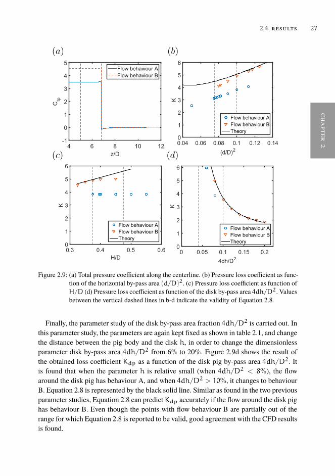
2.4.2 parameter study
In this section the parameters which govern the disk pig model are varied to investigatethe effect on the pressure loss coefficient K. Figure 2.9a shows the value of Ctp alongthe centreline of the disk pig shown in figure 2.8. The pressure loss coefficient K can nowreadily be determined:
K = Ctp,up −Ctp,down, (2.13)
whereCtp,up andCtp,down are the total pressure coefficients upstream and downstreamof the pig, respectively. As was already shown in the previous section, flow behaviour Bis associated with a higher loss coefficient compared to flow behaviour A, which amountsto a difference of 30%. The effect of the dimensionless parameter (d/D)2 on the twosolutions and on K is also investigated by changing (d/D)2 from 5% to 12.5%. Thisresult is shown in figure 2.9b. The two solution region was found to be in the region:
7.8% < (d
D)2 < 11.3%. (2.14)
More details on the exploration of the two solution region can be found in A. Furthermore,the values of K obtained from the CFD simulations are compared with the correlationgiven by Equation 2.8. Good agreement between the correlation for the disk pig and theCFD values was found, provided that the flow exhibits behaviour B.
Next, the effect of the disk diameter H is investigated through changing the dimen-sionless number H/D from 0.325 to 0.55, while keeping the other parameters fixed. Fig-ure 2.9c shows that when the disk has a relatively small disk height (when H/D < 0.35),the flow around the disk pig has behaviour B, while for H/D > 0.375, the flow aroundthe disk pig has behaviour A.The obtained CFD results are again compared with Equation 2.8 (the latter is repre-
sented by the black solid line in figure 2.9c). Similar as was found for the parametricstudy of the horizontal by-pass area it can be concluded that Equation 2.8 describes Kdpaccurately if the flow around the disk pig has behaviour B.WhenH/D is larger than 0.375and when the flow around the disk pig exhibits behaviour A, the pressure loss coefficientis found to have a constant value around Kdp = 3.83.
[ January 15, 2020 at 7:46 – classicthesis version 2.2 ]
chapter2
2.4 results 27
Figure 2.9: (a) Total pressure coefficient along the centerline. (b) Pressure loss coefficient as func-tion of the horizontal by-pass area (d/D)2. (c) Pressure loss coefficient as function ofH/D (d) Pressure loss coefficient as function of the disk by-pass area 4dh/D2. Valuesbetween the vertical dashed lines in b-d indicate the validity of Equation 2.8.
Finally, the parameter study of the disk by-pass area fraction 4dh/D2 is carried out. Inthis parameter study, the parameters are again kept fixed as shown in table 2.1, and changethe distance between the pig body and the disk h, in order to change the dimensionlessparameter disk by-pass area 4dh/D2 from 6% to 20%. Figure 2.9d shows the result ofthe obtained loss coefficient Kdp as a function of the disk pig by-pass area 4dh/D2. Itis found that when the parameter h is relative small (when 4dh/D2 < 8%), the flowaround the disk pig has behaviour A, and when 4dh/D2 > 10%, it changes to behaviourB. Equation 2.8 is represented by the black solid line. Similar as found in the two previousparameter studies, Equation 2.8 can predict Kdp accurately if the flow around the disk pighas behaviour B. Even though the points with flow behaviour B are partially out of therange for which Equation 2.8 is reported to be valid, good agreement with the CFD resultsis found.
[ January 15, 2020 at 7:46 – classicthesis version 2.2 ]

28 characterization of the pressure loss coefficient using a building block approach
chap
ter
2
Table 2.2: Key parameters that govern the speed controlled pig study.
Parameter Geometry 1 Geometry 2Horizontal by-pass area (%) 10% 30%By-pass pig diameter d 0.3668m 0.6354mUpstream pipe length Lup 2D 2DDistance between the pig body and the disk h 0.1118D 0.2236DDisk diameter H 0.4835D 0.7071DInner diameter holes Hi 0.4472D 0.4472DDisk thickness t 0.07071D 0.07071DNumber of holes n 4 4
2.4.3 speed controlled pig
This section is focused on the pressure drop coefficient of the speed controlled pig with thegeometry depicted in figure 2.5. For the speed controlled pig four by-pass adjusting holesare generated to represent the by-pass adjusting device (which gives the dimensionlessparameter n = 4). The angle of the by-pass adjusting holesω is changed to represent thespeed control process. Through changing ω the dimensionless number 4hHi(nω/360)
D2
is changed. This number represents the by-pass area fraction of the holes of the speedcontrolled pig. This dimensionless number is additional to the ones which already havebeen studied for the disk pig in the previous section. The effect of this dimensionlessnumber on the pressure loss coefficient of the speed controlled pig is studied for two basegeometries: one with a horizontal by-pass area of 10% and one with a horizontal by-passarea of 30%. The specific parameters of these two models are summarized in Table 2.2.The other parameters used in the simulation are unchanged with respect to the ones usedin the previous section and can be found in Table 2.1. The maximum opening angle of theby-pass holes is 45 degrees. This means that the total opening with 4 holes is 180 degreeswhich is the maximum that can be achieved with a rotating valve. The distance of the diskto the pig body is matched in such a way that for an opening angle ω = 45 degrees theby-pass area of the holes is equal to the horizontal by-pass area. When the holes close, theby-pass area of the holes decrease, and will be smaller than the horizontal by-pass area.This ensures that the main pressure drop occurs through the holes, which enables controlover the pressure loss as intended. As a consequence the maximum velocity in the systemwill always be located at the by-pass holes.
Figure 2.10 shows a typical result obtained for the flow around the speed controlled pig.This model has a horizontal by-pass area of 30% and the opening angle of the holes ωis 45 degrees. As can be seen from Figure 2.10a, the jets formed in the by-pass adjustingholes contact the pipe wall directly, and there is a recirculation zone both at the corner of
[ January 15, 2020 at 7:46 – classicthesis version 2.2 ]

chapter2
2.4 results 29
Figure 2.10: (a) Streamlines around the speed controlled pig. (b) Streamlines in the region of theby-pass holes. The dashed black line indicates the same position in both panels.
the pig body and at the pipe wall. This is thus similar to flow behaviour B for the disk pig.This flow behaviour is observed for all the cases which were investigated for the speedcontrolled pig. This is mainly due to the location of the disk, which is typically placed ata larger distance from the pig body for the speed controlled pig compared to the disk pig.The main recirculation zone is in the downstream pipe and is much more complex thanin the disk pig case. This is because there are four three-dimensional main jets formed inthe four by-pass adjusting holes, and when the jets bend around the disk, the jet-like flowmixes again in the downstream pipe. A close up of the jets emerging from the by-passholes is depicted in figure 2.10b. Similar to the disk pig, the main pressure drop occursat the exit of the by-pass pig, which is shown by the streamlines which are colour codedwith the value of the total pressure coefficient.
Next, a parameter variation of the two by-pass geometries listed in table 2.2 is carriedout. As the maximum velocity is always located in the holes it is intuitive to use this veloc-ity to scale the pressure drop coefficient. Note that until now, the velocity in the horizontalby-pass areaUbp has been used to scale the pressure drop. Therefore, a modified pressureloss coefficient K′ is defined which uses the velocity in the holes as a velocity scale. K′can thus be related to K as:
K′ =
[4hHi(nω/360)
d2
]2K. (2.15)
The parametric study is carried out by choosing the following values forω: 11.25, 22.5,37.75 and 45. The results are depicted in figure 2.11.It is noted that for ω = 45 the by-pass area of the holes is equal to the horizontal by-
pass area. In addition, the proposed correlation Equation 2.10 is included. This correlationis based on treating the speed controlled pig as an effective disk pig, as explained in sec-tion 2.2. The proposed correlation, despite the simplified approach, is able to predict the
[ January 15, 2020 at 7:46 – classicthesis version 2.2 ]

30 characterization of the pressure loss coefficient using a building block approach
chap
ter
2
[4hHi(nω/360)]/D
2
0 0.02 0.04 0.06 0.08 0.1
K′
0
1
2
3
4
CFD
Theory eqv. disk pig based on Hi
Theory eqv. disk pig based on H
[4hHi(nω/360)]/D
2
0 0.1 0.2 0.3
K′
0
1
2
3
4
CFD
Theory eqv. disk pig based on Hi
Theory eqv. disk pig based on H
Figure 2.11: (a) Pressure loss coefficient as function of the by-pass area fraction of the holes for ahorizontal by-pass area fraction of 0.1. (b) Pressure loss coefficient as function of theby-pass area fraction of the holes for a horizontal by-pass area fraction of 0.3.
right trend that is given by the CFD results. However, especially for lower values of theby-pass area, the suggested correlation overpredicts the results. Nonetheless the correla-tion can help to give a first estimation of the pressure loss coefficient of a speed controlledpig with a geometry as approximated by the schematic as shown in figure 2.5.
2.5 conclusions
In this chapter a building block approach was applied to describe the pressure loss coeffi-cient K of various by-pass pig geometries. First of all, K of the conventional bi-directionalby-pass pig has been revisited. Subsequently, new correlations for more complex geome-tries have been proposed and compared with CFD simulations using the building blockapproach. This building block approach allowed to construct correlations and for the diskpig geometry and the speed controlled pig geometery. A two solution region was foundfor the disk pig geometry, which means that there are two stable flow behaviours (type Aand type B) within the RANS framework of the current study. Good agreement was foundbetween the proposed correlation for the disk pig and the CFD results, provided that theflow exhibits flow behaviour B. In addition, the pressure loss coefficient of the speed con-trolled pig was characterized. It was found that a correlation based on an equivalent diskpig gives qualitatively the right trend, but deviates quantitatively for small opening anglesof the holes of the speed controlled pig. Further research is needed to predict K also forsmall opening angles of the holes. It is also of interest to further investigate the two solu-tion region that was found for the disk pig. The boundary of the two solution region maybe sensitive to the parameters of the RANS model, most notably the turbulence model.It would also be interesting to investigate the existence and stability of the two solution
[ January 15, 2020 at 7:46 – classicthesis version 2.2 ]
chapter2
2.5 conclusions 31
region experimentally in order to further verify the CFD modelling. The proposed build-ing block approach has been successfully applied to describe the pressure loss coefficientof various by-pass pig geometries, and may also be applied to systematically model thepressure loss coefficient of complex flow geometries in general.
[ January 15, 2020 at 7:46 – classicthesis version 2.2 ]

[ January 15, 2020 at 7:46 – classicthesis version 2.2 ]

chapter3
3FR ICT IONAL FORCES FOR D ISC -TYPE P IGG ING OFP I PEL INES
This chapter is adopted from M.H.W. Hendrix, C.M. Graafland, and R. van Ostayen, "Frictional forces fordisc-type pigging of pipelines". In: Journal of Petroleum Science and Engineering 171 (2018), pp. 905-918.
33
[ January 15, 2020 at 7:46 – classicthesis version 2.2 ]

34 frictional forces for disc-type pigging of pipelines
chap
ter
3
3.1 introduction
Pipelines that are used for the transport of fluids represent significant costs and need reg-ular maintenance [78, 79]. In the oil and gas industry this is usually done by sendingso-called pigs through the pipeline, see Figure 3.1a. Such a pig travels along with theproduction fluids through the pipe and can serve multiple maintenance purposes. For ex-ample pigs are used to remove wax particles that may have been deposited at the pipewall [74, 85, 94, 95] or to sweep out unwanted liquid accumulation in a pipeline that isused for multiphase gas-liquid transport [21, 96]. Apart from cleaning purposes, pigs canbe equipped with sensors which inspect the condition of the pipe wall. This is also referredto as intelligent pigging [63, 74]. For a detailed overview of pigging applications and pigtypes, the reader is referred to [15, 90]. In any case the pig is driven by the productionfluids which are transported through the pipeline. This means that the pressure differencethat is generated over the pig has to overcome the frictional force between the pig and thepipe wall. To ensure a safe and effective pigging operation it is thus required to know thefrictional force in order to prevent too high pressures in the system.
Figure 3.1: (a) A pig travelling inside a pipeline (b) Undeformed sealing disc. (c) Deformed sealingdisc.
A conventional pig completely seals the pipeline with a flexible sealing disc, see Fig-ure 3.1. The radius of the sealing disc usually has an oversize compared to the inner piperadius, which ensures a tight seal between the pig and the pipe wall. The travel velocityof a conventional pig through a pipeline is therefore equal to the mixture velocity of theupstream fluids. In some cases it is desired to lower the travel velocity of the pig, as it maycause damage to the pipeline or the pig itself. Also for cleaning, liquid removal, and in-spection purposes it is beneficial to reduce the pig velocity [12, 63, 91, 96]. A solution toachieve a lower pig velocity without causing production loss is the use of by-pass pigs [96].By-pass pigs have a by-pass hole which allows the production fluids to flow through the
[ January 15, 2020 at 7:46 – classicthesis version 2.2 ]

chapter3
3.1 introduction 35
pig. As a result the pig velocity is not dictated by the upstream mixture velocity anymore,but it is, in a horizontal pipe, determined by a balance of the by-passing fluid force andthe frictional force of the pig with the pipe wall. The force on a by-pass pig due to the by-passing fluids has been previously studied for various by-pass pig configurations, see [35,82]. The main focus of the current study is on the frictional forces which are encounteredduring pipeline pigging. As the pig contacts the pipe wall through the sealing disc, theeffect of the properties of the sealing disc on the frictional force is of interest. The exter-nal force of the pipe wall on the sealing disc is distributed along the circumference andhas unit Newton per meter circumference. The distributed force can be decomposed in adistributed friction force (F ′fric) oriented parallel to the direction of movement of the pigand a distributed wall normal force (F ′wall), as shown in Figure 3.1c. At the onset of slidingthe ratio of these two distributed forces gives the local Coulomb friction coefficient.Almost no models are available to estimate the frictional force during pipeline pigging:
predictions often rely on empirical findings and on field experience [14, 22]. For exampleCordell [14] presents a diagram in which the driving pressure that is needed to overcomethe frictional force is solely dependent on what type of pig is used (e.g. a cleaning pigversus an inspection pig). However, no information on the geometrical or material proper-ties of the sealing disc is present in this approach. O’Donoghue [70] presents a simplifiedmodel which does include geometrical and material properties of the sealing disc into afriction model. This model assumes that the deformed sealing disc adopts the shape ofan circular arc and subsequently evaluates the internal stresses in the sealing disc whichcan be used to predict the frictional force. Despite that the model contains more physicsthan for example Cordell’s model, it is known to systematically underpredict the frictionforce [34, 70]. Rather than relying on a simplified model, another approach is to performa full Finite Element (FE) calculation of the sealing disc, which has recently been un-dertaken in [99, 100]. Clearly, an axisymmetric 2D or even full 3D FE approach has theadvantage that it contains more physics than for example a simplified axisymmetric 1Dapproach, such as for example the model of O’Donoghue [70]. On the other hand, it ismore difficult to embed case specific FE calculations in already existing tools.Two types of laboratory approaches to experimentally study the frictional force of a
sealing disc have been found in the literature. One approach consists of a pull test in whicha sealing disc/pig is pulled through a pipe while monitoring the pulling force [100, 101].An advantage is that in steady state motion this pull force can be directly related to thefriction force. A disadvantage is that the wall normal force is not directly measured, andtherefore the Coulomb friction coefficient is unknown. Another approach relies on fixatingthe sealing disc while pressing it against a rotating steel plate which mimics the pipe wall,see [86] in which this setup was used to study wax removal from a pipe wall. Such a setupcan be used as a tribometer in which the load and friction force can be simultaneouslymeasured which enables to measure the friction coefficient for various contacts [52, 84].While the Coulomb friction coefficient can be carefully characterized with such a setup,
[ January 15, 2020 at 7:46 – classicthesis version 2.2 ]
36 frictional forces for disc-type pigging of pipelines
chap
ter
3
a disadvantage is that the friction force of a sealing disc in a confining pipe geometry isnot directly measured.
In the present research a static experimental setup is presented which is used to simul-taneously measure the friction force and the wall normal force acting on a sealing discin a confining pipe geometry. The static setup is a modified and improved version of thesetup described in [34], which will be explained in the Section 3.2. Six 12′′ off the shelfsealing discs from two different vendors have been used in the experiment. A flexiblehull is wrapped around the sealing disc and F ′wall is subsequently generated by reducingthe diameter of that hull. F ′fric is generated by pulling the disc in the axial direction. Theforces are recorded in static equilibrium. The forces that are applied in static equilibriumare the same as for a sealing disc that moves in steady state motion through a pipeline.By changing the force ratio between the friction force and the wall force the Coulombfriction coefficient which would apply to a sealing disc which moves at steady state isthus mimicked. The experimental setup thus allows to study the effect of the friction co-efficient which is difficult to study in a dynamic experiment in which a sealing disc ispulled through a pipe and the wall force is generally unknown. The results from the staticsetup, which is referred to as static pig pull facility, are captured by 2D axisymmetric FEcalculations for which appropriate boundary conditions are formulated. A detailed com-parison is made for both the involved forces as well as the shape of the deformed sealingdisc. Apart from the friction coefficient, the effect of the oversize, the thickness, and theYoung’s modulus of the sealing disc on the friction force are investigated.
Next to the static pig pull facility, a new dynamic pig pull experiment is designed whichis used to present a case example of how the results of the static pig pull facility can be re-lated to a dynamic pull test. In this dynamic experiment the sealing disc is pulled througha 1.7 meter vertical pipe while monitoring the pull force. The effect of possible lubri-cation by applying water at the sliding contact is investigated. The difference in frictioncoefficient between a dry and wet contact is quantified.The outline of this chapter is as follows. In Section 3.2 the experimental setup of the
static and the dynamic pig pull facility and the applied measurement procedure are ex-plained. At the end of the section the numerical setup for the FE calculations and theapplied boundary conditions are discussed. Section 3.3 presents the results from the staticpig pull facility and a direct comparison with the FE calculations is made. Subsequentlythe results from the dynamic pig pull facility are presented and linked to the results of thestatic experiments. Section 3.4 concludes and discusses possibilities for future research.
[ January 15, 2020 at 7:46 – classicthesis version 2.2 ]

chapter3
3.2 methods 37
3.2 methods
Inspecting Figure 3.1b we can identify two dimensionless numbers pertaining to the un-deformed geometry of the sealing disc. There is a dimensionless thickness t ′ and a dimen-sionless clamping ratio r ′p, which are defined as:
t ′ =t
rs − rp, (3.1)
r ′p =rp
rs. (3.2)
Here t is the thickness of the sealing disc, rs is the outer radius of the sealing disc, and rpis radius of the spacer discs which are used to attach the sealing disc to the pig body. Athird geometrical dimensionless number could take the presence of a possible chamfer intoaccount, see Figure 3.1b. The dimensionless chamfer height can be for instance definedas c ′ = c/t, where c is the length of the chamfer which is for simplicity assumed tobe under an angle of 45 degrees. The effect of a variation in chamfer size is discussedin Section 3.3.4. Two additional dimensionless numbers can be introduced for the sealingdisc which is deformed due to the confinement of the pipe wall, see Figure 3.1c. We definethe oversize parameter ∆ and the force ratio µ as follows:
∆ =rs − R
R× 100%, (3.3)
µ =F ′fricF ′wall
. (3.4)
Here R is the inner pipe radius, F ′fric is the distributed friction force and F ′wall is the dis-tributed wall normal force. Most sealing discs are made of polyurethane. This elastomerhas a high abrasion resistance, tear strength and resistance to hydrocarbons [70]. Thechemical composition of the sealing disc is proprietary to the manufacturer of the pig andit influences the Young’s modulus of the material, which is also referred to as E-modulus.The E-modulus is usually an input parameter for deformation models. Unfortunately, man-ufacturers do not specify the E-modulus of their product. Instead they specify the Shore Ahardness, which is a measure of the resistance of a material to indentation. Typical valuesfor the Shore A hardness of sealing discs are in the range of 60 - 85 [15].In this study a total of six sealing discs have been studied, see Table 3.1. These discs
have been obtained from two different pigging vendors, here anonymously named X andY. The discs from both vendors are intended for pigging of 12′′ pipelines. From vendor X,
[ January 15, 2020 at 7:46 – classicthesis version 2.2 ]

38 frictional forces for disc-type pigging of pipelines
chap
ter
3
Table 3.1: Overview of the sealing discs used in this study. Both the geometryand the material properties of the discs are listed. One set of spacerdiscs is used for all experiments (rp= 86 mm).
Disc A Disc B Disc C Disc D Disc E Disc FBatch X1 Y X2 X2 X2 X3rs (mm) 163.3 161.2 155.2 155.0 154.7 155.4t (mm) 15.9 15.2 13.6 15.5 17.4 15.4r ′p (-) 0.527 0.533 0.554 0.555 0.556 0.553
t ′ (-) 0.203 0.202 0.197 0.224 0.254 0.221Shore A hardness 75 (75.6)b 75 (79.6)b 75 75 75 65E-modulus (MPa) 8.5 13.7 10.1a 10.1 10.1a 6.0a The E-modulus of this disc is not obtained in a test, but assumed to be equal to theE-modulus of disc D. This disc is from the same batch as disc D, and only has adifferent thickness.
b Values as measured according to ASTM D2240, see Appendix B.
three different batches were obtained: X1, X2, and X3. The Shore hardness as specifiedby the manufacturer is listed. As the E-modulus was not specified it was determined bymaterial tests. These tests consisted of a stress strain analysis using representative dogbone samples from the disc. In addition to the stress strain tests, the Shore hardness ofdisc A and disc B was determined. A value of respectively 75.6 and 79.6 was found, whichare put in between brackets in Table 3.1. The value of disc A is within the specificationof the manufacturer, but the value of disc B is slightly higher. The details of the materialtests can be found in Appendix B. In any case it is clear that the value of the specifiedShore hardness cannot be used to deduce the E-modulus, for example by using the Gentequation [26], as discs with the same specified Shore hardness turn out to have differentvalues for the E-modulus. The radius of the spacer discs is kept constant in the experimentsand is equal to 86 mm. All experiments have been performed at room temperature.Disc A and disc B are the main discs that are used in our experiments. They have similar
properties except that they come from a different vendor and have a different E-modulus.Disc C, D, and E are from the same vendor and from the same batch. They have similarproperties, except for the variation in the thickness of the discs. These discs are used tostudy the effect of the thickness on the friction force. Discs C and disc F have similarproperties except for the E-modulus. These discs are thus used to study the effect of the E-modulus on the friction. The effect of the oversize ∆ and of force ratio µ are investigatedfor all the discs, as the experimental setup is designed to easily vary these parameters,which will be explained in the next section.
[ January 15, 2020 at 7:46 – classicthesis version 2.2 ]
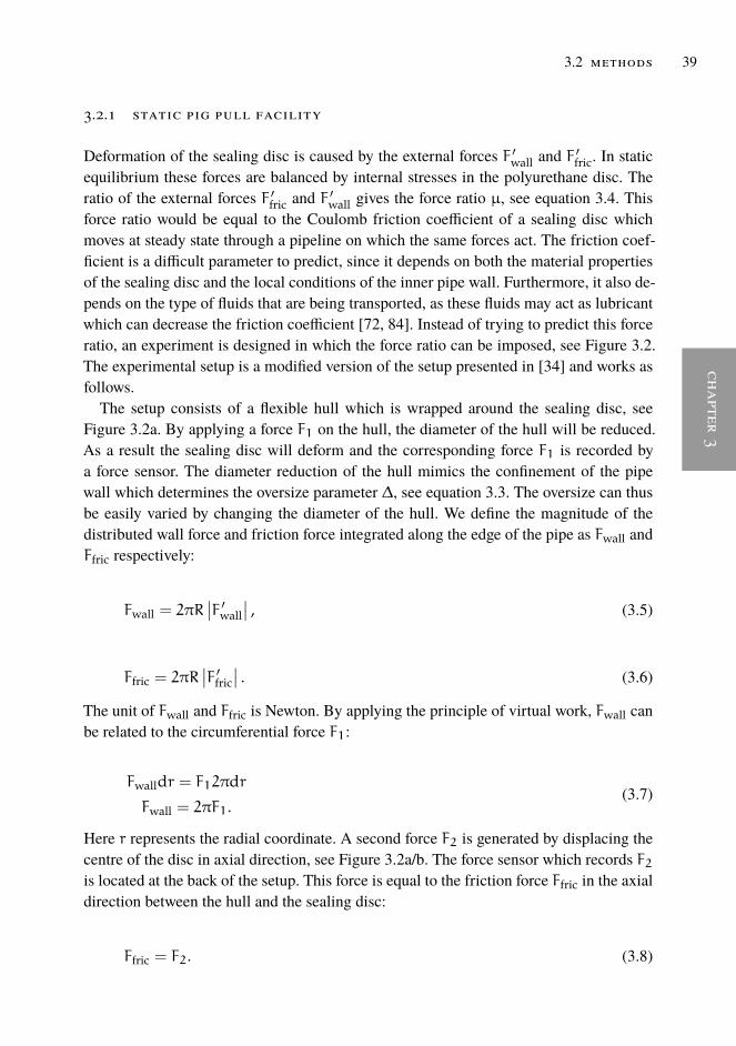
chapter3
3.2 methods 39
3.2.1 static pig pull facility
Deformation of the sealing disc is caused by the external forces F ′wall and F′fric. In static
equilibrium these forces are balanced by internal stresses in the polyurethane disc. Theratio of the external forces F ′fric and F ′wall gives the force ratio µ, see equation 3.4. Thisforce ratio would be equal to the Coulomb friction coefficient of a sealing disc whichmoves at steady state through a pipeline on which the same forces act. The friction coef-ficient is a difficult parameter to predict, since it depends on both the material propertiesof the sealing disc and the local conditions of the inner pipe wall. Furthermore, it also de-pends on the type of fluids that are being transported, as these fluids may act as lubricantwhich can decrease the friction coefficient [72, 84]. Instead of trying to predict this forceratio, an experiment is designed in which the force ratio can be imposed, see Figure 3.2.The experimental setup is a modified version of the setup presented in [34] and works asfollows.The setup consists of a flexible hull which is wrapped around the sealing disc, see
Figure 3.2a. By applying a force F1 on the hull, the diameter of the hull will be reduced.As a result the sealing disc will deform and the corresponding force F1 is recorded bya force sensor. The diameter reduction of the hull mimics the confinement of the pipewall which determines the oversize parameter ∆, see equation 3.3. The oversize can thusbe easily varied by changing the diameter of the hull. We define the magnitude of thedistributed wall force and friction force integrated along the edge of the pipe as Fwall andFfric respectively:
Fwall = 2πR∣∣F ′wall
∣∣ , (3.5)
Ffric = 2πR∣∣F ′fric
∣∣ . (3.6)
The unit of Fwall and Ffric is Newton. By applying the principle of virtual work, Fwall canbe related to the circumferential force F1:
Fwalldr = F12πdr
Fwall = 2πF1.(3.7)
Here r represents the radial coordinate. A second force F2 is generated by displacing thecentre of the disc in axial direction, see Figure 3.2a/b. The force sensor which records F2is located at the back of the setup. This force is equal to the friction force Ffric in the axialdirection between the hull and the sealing disc:
Ffric = F2. (3.8)
[ January 15, 2020 at 7:46 – classicthesis version 2.2 ]

40 frictional forces for disc-type pigging of pipelines
chap
ter
3
Figure 3.2: (a) Schematic of the setup. (b) Front view of the setup. (c) Side view of the setup. (d)Close-up of the steel ring and roller bearing.
The force ratio can now be expressed in terms of F1 and F2:
µ =Ffric
Fwall=
F22πF1
. (3.9)
By changing F2 and F1 the force ratio can be readily varied. In order to be able to obtainhigher values of the force ratio as compared to [34], a 2 mm steel ring has been weldedonto the hull in the circumferential direction, see Figure 3.2d. This ring prevents that thedisc slides in the axial direction when F2 is increased.
[ January 15, 2020 at 7:46 – classicthesis version 2.2 ]
chapter3
3.2 methods 41
A side view of the setup is shown in Figure 3.2c. Here it is visible that the back of theflexible hull is supported by roller bearings which are mounted on the frame. Figure 3.2dshows a close-up of one of the six roller bearings which are used. The addition of rollerbearings is an improvement compared the setup as presented in [34]. The roller bearingsensure that very little friction exists between the hull and the frame. This is especiallyimportant when the axial force F2 is increased, which effectively pushes the hull againstthe roller bearings. Without the roller bearings a friction force between the hull and theframe could exist which would result in an under prediction in the value of F1. The setupis operated in such a way that static equilibrium is reached. The corresponding values forFfric and Fwall in this static situation represent the same force balance that would apply toa sealing disc on a pig that moves in steady state motion in a pipeline.
Figure 3.3: (a) Profile comb. (b) Deformation extracted from the profile comb.
Next to the forces that act on the sealing disc also the deformation of the sealing disc ismeasured. This is done by mounting a profile comb on the spacer disc, see Figure 3.3. Theprofile comb is subsequently pressed against the sealing disc in order to measure the shape.The rotation of the profile comb can be adjusted which allows to measure the deformationat different positions. Deformation measurements in addition to force measurements pro-vide a more complete set of results compared to force measurements alone, as was donein [34]. Figure 3.3a shows the profile comb in a 3 o’clock position, but also the 12 o’clockand 6 o’clock position have been employed. These different positions allow to verify ifthe deformation of the sealing disc is axisymmeteric. A camera holder is used to take aphoto in the same plane as the profile comb. Subsequently the deformation is obtained byextracting the position of the pins using image processing. The detected location of the
[ January 15, 2020 at 7:46 – classicthesis version 2.2 ]

42 frictional forces for disc-type pigging of pipelines
chap
ter
3
pins is shown by the red dots in Figure 3.3b. Even though this study focuses on pigs witha sealing disc, the experimental setup could be used to study other types of pigs, such aspigs with cups or foam pigs [74]. In case of foam pigs it however makes less sense to at-tempt to measure any deformation in axial direction, as a foam pig is mainly compressedin radial direction. In the next section the measurement procedure and a typical resultobtained from the force sensors are discussed.
3.2.1.1 Measurement procedure
The measurements were performed with two 24-bit GSV-2TSD-DI data acquisition de-vices connected to a 1 kN and 2 kN load cell (KD40S, ME-Systeme) which record thecircumferential force F1 and the axial force F2, respectively. The measurements were per-formed at a sample frequency of 10 Hz and logged onto a computer. The procedure ofa typical measurement is as follows. First, the disc is brought to a specific oversize byapplying a force F1 which reduces the diameter of the hull. The oversize is kept fixedwithin one experiment. Subsequently, the disc is step-wise displaced in axial direction re-sulting in a force F2. One step corresponds to a rotation of the screw that can be seen inFigure 3.2b. The lead of the screw is 1.5 mm. One rotation is made in approximately 30seconds to maintain static equilibrium. The axial force F2 is increased up to a predeter-mined maximumwhich is just below the value which would result in the disc moving overthe steel ring, see Figure 3.2d. After reaching a maximum value, F2 is decreased in stepsto come back at a value of 0 N. This procedure is repeated three times per measurement.Figure 3.4a shows one typical time series of measurement data which were obtained byapplying the procedure to disc B subjected to an oversize ∆ = 4%.Figure 3.4a clearly shows the stepwise behaviour in the forces, which corresponds to
the stepwise adjustment of F2 as explained above. It is noted that an increase in F2 corre-sponds to a decrease in F1 and vice versa. This is expected as the disc is not only deformedby a wall normal force (related to F1), but also by a friction force (equal to F2). The cor-responding value of the force ratio µ according to equation 3.9 is included in Figure 3.4a.For the axial force F2 three zones can be distinguished: a rise zone, where F2 increases, arest zone, where F2 does not change and a relax zone, where F2 decreases. The rest zonelasts longer and is noisier compared to when F2 is increasing, because here the profilecomb is used to determine the deformation at three different positions on the sealing disc:12 o’clock, 3 o’clock and 6 o’clock.
Figure 3.4b shows an alternative way of plotting the same data. The forces F1 and F2are now plotted as function of µ. The data are colour coded to distinguish between therise, relax, and rest zones. In this plot now all three time series of the measurement areincluded. The inset in Figure 3.4b shows a close up of the data. The data from the threedata sets are very close to each other, which thus confirms the excellent reproducibilityof the experiment. It can also be seen that the data from the relax zone, as shown in blue,
[ January 15, 2020 at 7:46 – classicthesis version 2.2 ]
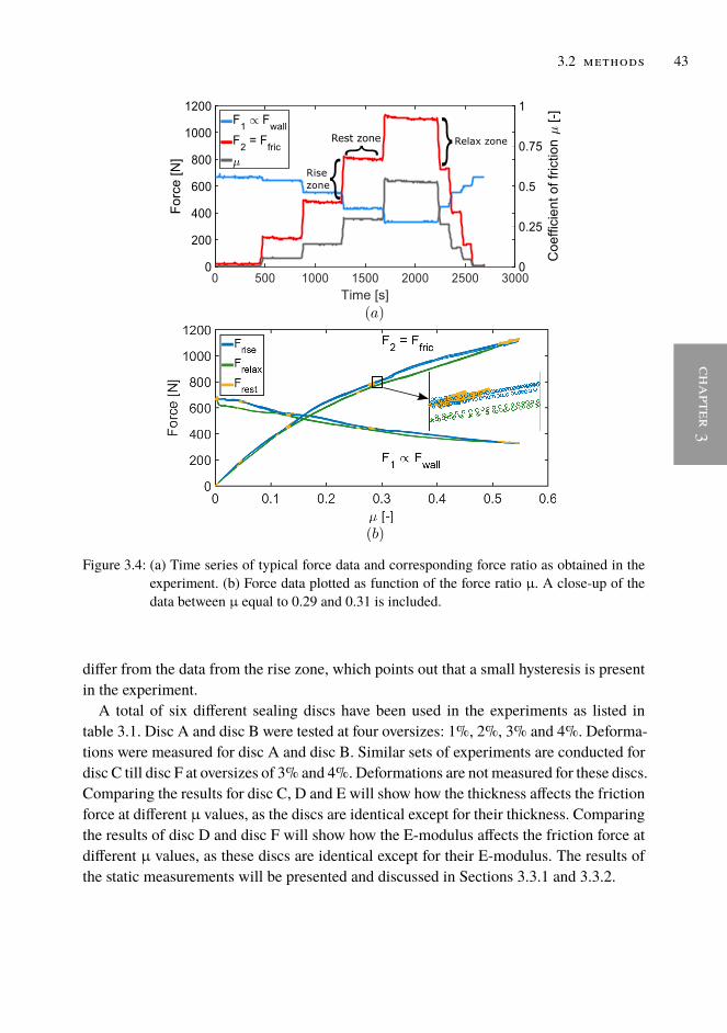
chapter3
3.2 methods 43
Figure 3.4: (a) Time series of typical force data and corresponding force ratio as obtained in theexperiment. (b) Force data plotted as function of the force ratio µ. A close-up of thedata between µ equal to 0.29 and 0.31 is included.
differ from the data from the rise zone, which points out that a small hysteresis is presentin the experiment.A total of six different sealing discs have been used in the experiments as listed in
table 3.1. Disc A and disc B were tested at four oversizes: 1%, 2%, 3% and 4%. Deforma-tions were measured for disc A and disc B. Similar sets of experiments are conducted fordisc C till disc F at oversizes of 3% and 4%. Deformations are not measured for these discs.Comparing the results for disc C, D and E will show how the thickness affects the frictionforce at different µ values, as the discs are identical except for their thickness. Comparingthe results of disc D and disc F will show how the E-modulus affects the friction force atdifferent µ values, as these discs are identical except for their E-modulus. The results ofthe static measurements will be presented and discussed in Sections 3.3.1 and 3.3.2.
[ January 15, 2020 at 7:46 – classicthesis version 2.2 ]

44 frictional forces for disc-type pigging of pipelines
chap
ter
3
3.2.2 dynamic pig pull facility
To study the dynamic friction force a new dynamic pig pull facility has been designed,see Figure 3.5. The setup consists of a 1.7 m vertical carbon steel pipe through which asealing disc can be pulled at a preset velocity using a linear actuator. The inner radius ofthe pipe is 157 mm. The linear actuator (Thomson, ECT130) is connected to a brushlessAC servomotor (AKM63), which is located at the top end of the pipe. The actuator is ableto translate a spindle which has a total length of 2 m and a lead of 20 mm. At the lowerend of the spindle a 5 kN load cell (AXH Scaime) is connected to which the sealing disc isattached, see Figure 3.5a/b. The load cell is able to directly measure the propulsive forcewhich is needed to pull the sealing disc through the pipe. Simultaneously the position,velocity and acceleration are monitored with a logging frequency of 200 Hz. The speedof the sealing disc can be varied between 5 and 300mm/s. The pipeline is placed verticallywhich makes it possible to add liquids uniformly on top of the sealing disc, see Figure 3.5a.Herewith the effect of possible lubrication on the frictional force caused by the presenceof a liquid can be investigated. For a sealing disc moving in an upwards direction in thepipe, the steady state force balance reads:
Fm = Ffric + Fg, (3.10)
where Fm is the propulsive force of the servomotor, Ffric is the friction force between thesealing disc and the pipe wall and Fg is the gravitational force. In dry experiments Fg isdue to the mass of the sealing disc and of the spacer discs. In wet experiments also themass of the lubricant supply on top of the disc has to be taken into account.A by-pass is created by drilling three holes in the spacer discs, see Figure 3.5a. For the
wet experiments, this allows the lubricant to flow through the disc into the leakage traywhen the liquid level equals the height of the upper spacer disc. With a minimum amountof lubricant a wet sliding contact can be obtained.
3.2.3 measurement procedure
Rather than a parameter study, as is conducted with the static pig pull facility, only onedisc (disc A) is used in the dynamic pig pull experiments as case study. A measurementcommences with the spindle in its most extended position with the sealing disc mountedon it (approximately 30 cm below the pipe), see Figure 3.5b. This is called the homeposition of the disc. From here the sealing disc is pulled slowly at a velocity of 5 mm/s tothe initial position, which is 50 mm into the pipe. The disc is kept in this position for 60seconds to make sure that possible settling effects are no longer present. After this delaytime the actual pull test begins and the disc accelerates, moves up through the pipe at thepreset velocity, and then decelerates until rest in its final position at the top of the pipe.
[ January 15, 2020 at 7:46 – classicthesis version 2.2 ]

chapter3
3.2 methods 45
Figure 3.5: (a) Schematic of the dynamic pig pull facility (b) Photograph of the dynamic pig pullfacility
Three preset velocities have been used: 100, 200, and 300 mm/s. The spindle accelerationand deacceleration are set to 100 mm/s2. When the disc is moving up, both the motion(position, velocity, and acceleration) and the propulsive force are monitored. No data arelogged when the disc moves back down, as only pull tests are considered in this study.In the wet experiments an additional step is added to the procedure. After the disc is
positioned in the start position, water is inserted from a small tap at the top of the pipelineuntil it starts leaking through the by-pass holes, see Figure 3.5a. The top part of the sealingdisc and the adjacent pipe wall are now wetted. Subsequently, the tap is closed and theleakage tray is emptied before it is put back under the pipe. The pull test can now begin.When the disc is moving upwards the water leaking past the sealing disc or through theby-pass holes is negligible. In this way it is thus possible to create a wet contact betweenthe pipe wall and the sealing disc. At the end of the pull test the disc is returned back to itsstart position. When the disc starts moving down it buckles to the opposite side and as aresult the water flows through the by-pass holes and is collected into the leakage tray. Themass of the water (approximately 1 litre in volume) is determined and used in the forcebalance, see Equation 3.10. In this study only water is used as lubricant.The two spacer discs are separated by a small length of tube, and this tube therefore
determines how tight the sealing disc is clamped between the spacer discs. Three config-urations are created by selecting three values for the length L of the tube which is shownFigure 3.5b. To the best knowledge of the authors the effect of this parameter on the fric-tional force of a sealing disc of a pig has not been reported in previous studies. As willbecome clear in Section 3.3.3 the length L of the tube influences the outer diameter of thesealing disc, and therefore the oversize, due to the nearly incompressible behaviour of thepolyurethane. For all three configurations wet and dry experiments are conducted at vary-ing speeds. Each separate experiment is repeated five times for reproducibility purposes;
[ January 15, 2020 at 7:46 – classicthesis version 2.2 ]

46 frictional forces for disc-type pigging of pipelines
chap
ter
3
the first two runs are used to mitigate any settling effects of the disc and the last three runsare used in the actual analysis. Next to the varation of L the disc is placed in both a faceup and face down orientation to investigate the presence of any possible asymmetries.
3.2.4 finite element model
Comsol Multiphysics (version 5.2) is used in this study for the Finite Element (FE) analy-sis. We solve the structural mechanics problem in which we solve for the deformation ofthe sealing disc which is caused by the wall force and the friction force which act on thechamfer of the sealing disc, see Figure 3.6. We consider static equilibrium, in which caseNewton’s second law reads:
∇ · σ = 0. (3.11)
Here σ is the Cauchy stress tensor. The stresses are calculated using a linear isotropicmaterial model. The E-modulus which is used has been determined by material tests andcan be found in Table 3.1. The Poisson’s ratio ν is taken equal to 0.49. Since the typicaldeformation which occurs can be in the order of a few times the thickness of the sealingdisc, a nonlinear geometry model is used. We assume an axisymmetric geometric model.Figure 3.6 shows the typical mesh which is used for the calculations. Second order
quadratic elements are used. The meshing is adapted on the thickness of the disc to guar-antee appropriate meshing for both thick and for thin discs. In the thickness direction thesize of the element is controlled between a minimum size of t/6 and a maximum size of 1.2times t/6. In the radial direction the edges have a length equal to the edges in the thicknessdirection multiplied by a factor 1.5. The mesh consists of approximately 400 elements,which was verified to be sufficiently fine by making a comparison with simulation resultswith a smaller number of elements.
The green lines in Figure 3.6 represent roller boundary conditions on both sides of thesealing disc between r = 0 and r = rp, due to the spacer discs. Here the sealing disc isconstrained to move in the normal direction, but it is allowed to move parallel to the spacerdiscs. The freedom to move, however, is limited, due to the axisymmetric geometry. It wasfound that this boundary condition is appropriate to model the confinement of the spacerdiscs, even though a finite, non-zero clamping force of the spacer discs on the sealingdisc exists. An alternative boundary condition could be a completely clamped boundarycondition [69], which would prohibit any movement of the disc in the region of the spacerdiscs. This was found to be unsuitable, as a finite deformation was observed in the regionof the spacer discs, which will become clear in Section 3.3. The blue square representsthe chamfer of the disc, where the wall force and the friction force act. The chamfer sizec is set to 1.4 mm, as measured from the sealing disc. The remaining edges have a freeboundary condition.
[ January 15, 2020 at 7:46 – classicthesis version 2.2 ]

chapter3
3.3 results 47
Figure 3.6: Geometry and boundary conditions of the finite element model. (a) Initial geometry.(b) Deformed geometry. (c) Typical simulation result.
For low µ values high wall forces are involved when a sealing disc is confined inside apipe. In reality and in the experiments in this study a sealing disc automatically bucklesbackwards with respect to the moving direction. To ensure that in the FE model the discbuckles to the correct side the FE model is solved in multiple steps. First the friction forceis added and then the wall force is increased in steps to its final value. Within the solutionprocess, the result of the previous calculation step is used as an initial condition for thenext calculation step. This helps to buckle the disc in the direction of the friction force.Figure 3.6c shows a typical simulation result of disc A subjected to a wall force Fwall =400 N and a friction force Ffric = 200 N. The interior of the disc is color coded by the vonMises stress. High stress points typically occur near the outer edge of the spacer discs.
3.3 results
In this section the results are presented which are obtained by the methods described inthe previous Section 3.2. First the results from the static experiment are presented. InSection 3.3.1 the deformations obtained in the experiments and the deformations foundusing the FE model are compared for disc A and disc B, see Table 3.1. In Section 3.3.2 thefriction force as a function of µ and oversize is shown, both for disc A and for disc B. Inaddition, Section 3.3.2 shows the friction force for different values of the E-modulus andthe thickness of the disc. For this purpose discs C to F are used. Section 3.3.3 present the
[ January 15, 2020 at 7:46 – classicthesis version 2.2 ]

48 frictional forces for disc-type pigging of pipelines
chap
ter
3
results which are obtained with the dynamic pig pull experiment. Section 3.3.4 discusseshow the results from the static and dynamic pig pull experiments are related.
3.3.1 shape comparison
We have obtained the shape of the sealing disc using the deformation device as describedin Section 3.2.1. Figure 3.7 shows the results for disc A subjected to 3% oversize. InFigure 3.7a a time series is shown, where the blue line denotes the wall force Fwall andthe red line denotes the friction force Ffric. In the first five rest zones, where the forcesare constant, the deformation of the disc is measured. To show how the measured shapescompare with the FE model, data from the last three rest zones are shown in Figure 3.7b-d.The last three rest zones which correspond to sub-figure b-d are indicated in Figure 3.7a.
Figure 3.7: Experimental results for disc A at 3% oversize. The black dotted shape in sub-figuresb-d represents the FE model. (a) A time series showing the wall force and the frictionforce. Deformations are measured in the rest zones labeled b-d. (b) Fwall = 1908 N andFfric = 266 N. (c) Fwall = 1429 N and Ffric = 439 N. (d) Fwall = 977 N and Ffric = 620N.
It can be seen that the FE results, which are shown by the black dots, agree very wellwith the average measured deformation. The FE results were obtained by applying theforces that were measured in the experiment to the chamfer of the disc in the FE model,as described in Section 3.2.4. It can also be noted from the measured data that the sealing
[ January 15, 2020 at 7:46 – classicthesis version 2.2 ]

chapter3
3.3 results 49
disc does not deform perfectly axisymmetrically in the hull. The largest deflection occurswhen the deformation device is at 6 o’clock, followed by 3 o’clock and 12 o’clock. Thisis a consequence of the position of the tensioning mechanism located at 6 o’clock, seeFigure 3.2a. This breaks the axisymmetry of the hull, resulting in a slightly non perfectcircular shape. No attempt has been made to correct this, since adding new forces to thesystem was not desired. The gravity force is assumed to play a minor role as it is only asmall fraction of the encountered wall forces.In Figure 3.7b-d the force ratio µ varies from 0.14 to 0.64 which corresponds to a
substantial variation in Fwall and Ffric, see Figure 3.7a. The deformation of the disc duringthis process, however, only changes slightly. Both the measured data from the deformationdevice and the FE model show this behaviour. This means that there exists approximatelyone axisymmetric shape of the sealing disc which is fitted in a pipe, and that the effect ofµ on the final shape is only minor. As was discussed in Section 3.2.4 a roller boundarycondition was chosen to represent the confinement of the spacer discs. It can be clearlyseen that the angle of deformation is not zero at the radius of the spacer disc r = rp,which supports the choice of a roller boundary condition over a fully clamped boundarycondition.The deformation results for disc A at 3% oversize were shown in Figure 3.7 as case
example. The deformations results of disc A for all oversizes 1%, 2%, 3%, and 4% arepresented in Figure 3.8a. Here the maximum deformationwmax, which occurs at the tipof the disc is selected, see Figure 3.7d, and is plotted as function of µ.The experimental data in Figure 3.8a are plotted as error bars in different colours which
correspond to different oversizes. The lower and upper limit of the error bar representthe deformation measurements at 12 o’clock and 6 o’clock, respectively, while the maindata point (open circle) of the error bar represents 3 o’clock, see Figure 3.7. The greenerror bars connected with the black line in Figure 3.8a link to the deformation resultsin Figure 3.7, as here an oversize of 3% was shown. The black line shows that wmaxonly increases by a few millimetres while µ increases significantly. At every oversize theexperiment was conducted three times. The fact that the three corresponding error barsare lying on top of each other indicates that the experiment is reproducible. The sameprocedure was applied to disc B. These results are summarized in Figure 3.8b. It canbe concluded that the FE model is able to predict the shapes and wmax obtained in theexperiment. Only for small µ no FE data are plotted. Here the FE model returns a solutionbuckled to the other side. In general it is found that µ does not have a large effect on howthe disc is fitted in the pipeline. It is evident that the oversize does have a large effect onthe shape, as a larger oversize means that the disc has to deform more to fit in the pipe.The length of the error bars in Figure 3.8b is longer, indicating that there is a larger spreadbetween the deformation measurements at 3, 6 and 12 o’clock. This can be explained bythe larger E-modulus of disc B, as this stiffer disc is more sensitive to any asymmetriesin the setup. The results in Figure 3.7 and Figure 3.8 are obtained without using a fittingparameter for the E-modulus. The E-modulus used in the FE model is shown in Table 3.1
[ January 15, 2020 at 7:46 – classicthesis version 2.2 ]

50 frictional forces for disc-type pigging of pipelines
chap
ter
3
Figure 3.8: Comparison of wmax in the experiments and in the FE model for different oversizes.(a) Disc A. (b) Disc B.
and is obtained in stress and strain tests as described in Table 3.1. In the next sectionvarious parametric studies are described, in which also the effect of a variation in theE-modulus on the friction force is discussed.
3.3.2 parameter study
Figure 3.9 shows the friction force in the rise and rest zones as function of the force ratioµ for the four oversizes for disc A and disc B. The corresponding wall force Fwall can beobtained as the ratio of Ffric and µ.A first inspection of Figure 3.9 shows that the friction force of disc B is overall higher
than the friction force of disc A. This is a consequence of the higher E-modulus of discB compared to disc A, see Table 3.1. The maximum µ values obtained differ per oversizeand per disc, indicating that the discs start to move over the steel ring (Figure 3.2) at a
[ January 15, 2020 at 7:46 – classicthesis version 2.2 ]

chapter3
3.3 results 51
Figure 3.9: (a) Friction force as a function of µ for different oversizes for disc A (b) Idem disc B.(c) The friction force as a function of the oversize for disc A (d) Idem disc B.
different critical value of µ. The generic trends observed for all oversizes are similar forboth discs. We focus on the µ regime between 0.2 and 0.6.In the chosen µ regime also FE simulation results are shown in black. The black lines
are fitted through 10 data points. For these data points at different µ the friction force (andthus the wall force as µ is fixed) is increased until the FE model reaches the same oversize(1-4%) as in the experiment. The shaded regions around the black lines show the resultsof a variation by ±5% of the E-modulus used in the FE model.
The friction forces necessary to bring the disc in the desired oversize in the FE modelcorrespond very well to the experiments. Both the trend and the actual magnitudes arecaptured accurately by the FE model. Figure 3.9a shows that the experimental resultsand the FE results agree very well for disc A with oversizes 2% and 3%. The FE modelpredicts a lower friction force to bring the disc in 4% oversize. The maximum deviation at4% oversize is only 9.3%. At 1% oversize no experimental data are available in the chosenµ regime. For disc B, shown in Figure 3.9b, the results are in agreement for the 1% and2% oversizes. For the 3% and 4% oversizes the FE model underpredicts the friction force,with a maximum underprediction by 5.2% and 11.6%, respectively.
[ January 15, 2020 at 7:46 – classicthesis version 2.2 ]
52 frictional forces for disc-type pigging of pipelines
chap
ter
3
Both Figure 3.9a and Figure 3.9b show that the experimental friction force data areapproximately evenly spaced when the oversize increases from 1% to 4%. For the FEdata the increase in friction force seems to decrease as the oversize increases. A reasonfor this difference in behaviour might be that the wall force is incorrectly captured athigher oversizes (and thus higher friction forces) in the experiments. To capture the wallforce correctly six ball bearings were added to the setup, see Section 3.2.1. This was tomake sure that no undesired forces were added in the plane of the hull, affecting F1. Forhigh friction forces the contact between the hull and the ball bearings connected to theframe may still not be completely frictionless. Undesired friction between the hull andthe frame is difficult to prevent completely. Therefore the force sensor monitoring F1 mayoverpredict the wall force. This means thatµ is underpredicted for the experimental data inFigure 3.9. There is no reason to assume that the experiment does not capture the frictionforce correctly. When this hypothesis is true the experimental data would shift to the rightfor high friction forces. Intuitively, the FE data make sense as one may expect that it iseasier to increase the oversize from 3% to 4% than from 1% to 2%. This is also what hasbeen observed in other research [69, 100]. To directly see the effect of the oversize on thefriction three values of µ have been highlighted in Figure 3.9a and b. Along these linesof constant µ experimental data have been gathered in a range between µ + 0.002 andµ− 0.002. The error bar represents the standard deviation of the data within this range.Disc D and disc F are tested to see how the friction force behaves as a function of the E-
modulus. Figure 3.10a shows the results when the disc is at 3% oversize and Figure 3.10bfor 4% oversize. The discs have similar specifications except for the Shore hardness andthe E-modulus, see Table 3.1. The thickness and the sealing disc radius are not exactly thesame; therefore in the FE model the average thickness and radius are selected. The resultsare shown for three different values for µ. For the disc with the lower Shore hardnessand E-modulus (disc F) the experimental data agree very well with the FE data for allthree values of µ. The maximum deviation in friction force between the FE results andthe experiments equals 6.5%. The results of the experiments with the stiffer disc showhigher friction forces than predicted by the FE model, especially at 4% oversize. Themaximum deviation in friction force between the FE results and the experiments equals14.7%. This is in line with the observation in the previous section that Fwall is not capturedcorrectly in the experiment for high friction forces. When Fwall is overpredicted, µ isunderpredicted. Figure 3.10 shows that lower µ values would correspond to a smallergradient in the experimental data. It is worthmentioning that the experimental setup whichis designed can actually serve as a tool to predict the E-modulus of a sealing disc in a nondestructive way by fitting the experimental data on the FE results.Disc C, disc D and disc E are tested to see how the friction force behaves as a function
of the disc thickness. The discs have the same manufacturer and are from the same batch.Only the thickness of the discs is different, see Table 3.1. Therefore the E-modulus of discC and disc E have not been obtained in a stress and strain test, but are assumed to be equalto the E-modulus of disc D. Figure 3.10c shows the friction force with µ being equal to
[ January 15, 2020 at 7:46 – classicthesis version 2.2 ]

chapter3
3.3 results 53
Figure 3.10: The black line represents results from FE calculations. (a) The friction force as afunction of the E-modulus at 3% oversize. (b) The friction force as a function of theE-modulus at 4% oversize. The experimental results are compared to the FE results atthree µ values: 0.24, 0.42 and 0.6. (c) The friction force as a function of the thicknessat µ equal to 0.42. (d) The friction force as a function of the thickness at µ equalto 0.6. Disc C, disc D and disc E are tested at 3% and 4% oversize. The FE resultscorrespond to, from top to bottom, 4%, 3%, 2% and 1% oversize.
0.42. Experimental data are shown at 3% and 4% oversize. The FE model is shown for anoversize of 1%, 2%, 3% and 4%. The maximum deviation in friction force between the FEresults and the experiments equals 18.1%. This deviation occurs for disc C at 4% oversize.Figure 3.10d shows similar data with µ equal to 0.6. Here the maximum deviation infriction force between the FE results and the experiments equals 11.2%, also occurringfor disc C at 4% oversize. For the two thicker discs the FE model agrees very closely withthe experimental data while the friction forces for the thinnest disc are underpredicted.
3.3.3 results from dynamic pig pull experiments
In this section the experimental results from the dynamic pig pull experiments are pre-sented. All experiments are conducted with disc A. As was discussed in Section 3.2.3the length of the tubes L which defines the distance between the spacer discs was varied.Thereby the clamping force of the spacer discs which squeezes the sealing disc is varied.
[ January 15, 2020 at 7:46 – classicthesis version 2.2 ]

54 frictional forces for disc-type pigging of pipelines
chap
ter
3
The reduction in the length compared to the original length when the clamping force iszero is defined L ′. Three values for L ′ have been studied: 0, 1, and 2 mm. As the originalthickness of disc A is equal to 15.9 mm (see Table 3.1), values of L ′ equal to 0,1, and 2mmcorrespond to a compression of 0%, 6%, and 13% respectively. The compression in theaxial direction causes the disc to expand in radial direction, due to the nearly incompress-ible behaviour of polyurethane. As a result the outer diameter increases. This has beenquantified, see Table 3.2. Here it can be seen that for L ′ = 0 the original radius of the discequals rs = 162.2 mm. As the inner radius of the pipe is 157 mm, this corresponds to anoversize of ∆ = 3.33%. Upon increasing the clamping force by increasing L ′ the radiusand corresponding oversize thus increase.
Table 3.2: Oversizes before and after a first pull test.
L ′ [mm] Before pull test After pull testrs [mm] ∆ [-] rs [mm] ∆ [-]
0 162.2 3.33 162.2 3.331 162.7 3.64 162.9 3.742 163.3 4.04 163.7 4.24
For the tubes that squeezed the disc by 1 mm or 2 mm the disc oversizes were slightlyhigher after a first pull test, compared to the oversize measured directly after assemblingthe spacer discs on the sealing disc. For the tubes that were not squeezing the disc (L ′ =0 mm) this phenomenon was not observed. This indicates that a small settling effect ispresent which can be explained by the forces that occur in the experiment that are able topull the disc radially outward. When the clamping force is zero (L ′ = 0) the disc is ableto retract to its original position, but with a non zero clamping force (L ′ = 1 and L ′ = 2)the disc remains radially extended. This settling effect is not investigated further in thiswork.
The effect of L ′ on the frictional force is investigated for various disc speeds. Also theeffect of a dry versus a wet contact is investigated, as described in Section 3.2.3. Theexperiments and corresponding parameters are summarized in Table 3.3. Here it is alsoshown that also a face up and face down orientation of the disc is distinguished. Theaverage values of the force data are listed as found when the disc is moving at constantvelocity, as described in Section 3.2.3. The sequence of the experimental runs can bededucted from the table: first the runs without squeezing are conducted, followed by theruns with 1 mm and 2 mm squeezing. For one set of tubes we start with the dry runs: firstfive runs at 100 mm/s followed by five runs at 200 mm/s and 300 mm/s. After this, the dryface down, wet face down and wet face up runs are performed. Before the experimentswith the next set of tubes are conducted, the setup is left for an entire day to dry. Theexperiments in Table 3.3 correspond to approximately 600 m of pipeline pigging (threesets of tubes, four configurations, three speeds, five repetitions, 3.2 m between subsequent
[ January 15, 2020 at 7:46 – classicthesis version 2.2 ]
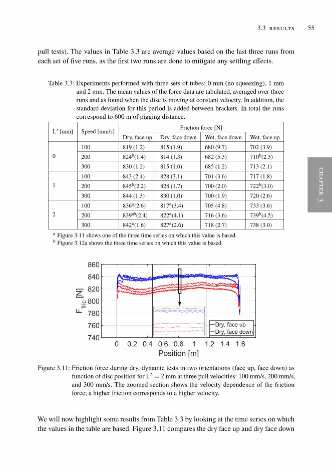
chapter3
3.3 results 55
pull tests). The values in Table 3.3 are average values based on the last three runs fromeach set of five runs, as the first two runs are done to mitigate any settling effects.
Table 3.3: Experiments performed with three sets of tubes: 0 mm (no squeezing), 1 mmand 2 mm. The mean values of the force data are tabulated, averaged over threeruns and as found when the disc is moving at constant velocity. In addition, thestandard deviation for this period is added between brackets. In total the runscorrespond to 600 m of pigging distance.
L ′ [mm] Speed [mm/s] Friction force [N]Dry, face up Dry, face down Wet, face down Wet, face up
0100 819 (1.2) 815 (1.9) 680 (9.7) 702 (3.9)200 824b(1.4) 814 (1.3) 682 (5.3) 710b(2.3)300 830 (1.2) 815 (1.0) 685 (1.2) 713 (2.1)
1100 843 (2.4) 828 (3.1) 701 (3.6) 717 (1.8)200 845b(2.2) 828 (1.7) 700 (2.0) 722b(3.0)300 844 (1.3) 830 (1.0) 700 (1.9) 720 (2.6)
2100 836a(2.6) 817a(3.4) 705 (4.8) 733 (3.6)200 839ab(2.4) 822a(4.1) 716 (3.6) 739b(4.5)300 842a(1.6) 827a(2.6) 718 (2.7) 738 (3.0)
a Figure 3.11 shows one of the three time series on which this value is based.b Figure 3.12a shows the three time series on which this value is based.
Figure 3.11: Friction force during dry, dynamic tests in two orientations (face up, face down) asfunction of disc position for L ′ = 2mm at three pull velocities: 100 mm/s, 200 mm/s,and 300 mm/s. The zoomed section shows the velocity dependence of the frictionforce; a higher friction corresponds to a higher velocity.
We will now highlight some results from Table 3.3 by looking at the time series on whichthe values in the table are based. Figure 3.11 compares the dry face up and dry face down
[ January 15, 2020 at 7:46 – classicthesis version 2.2 ]
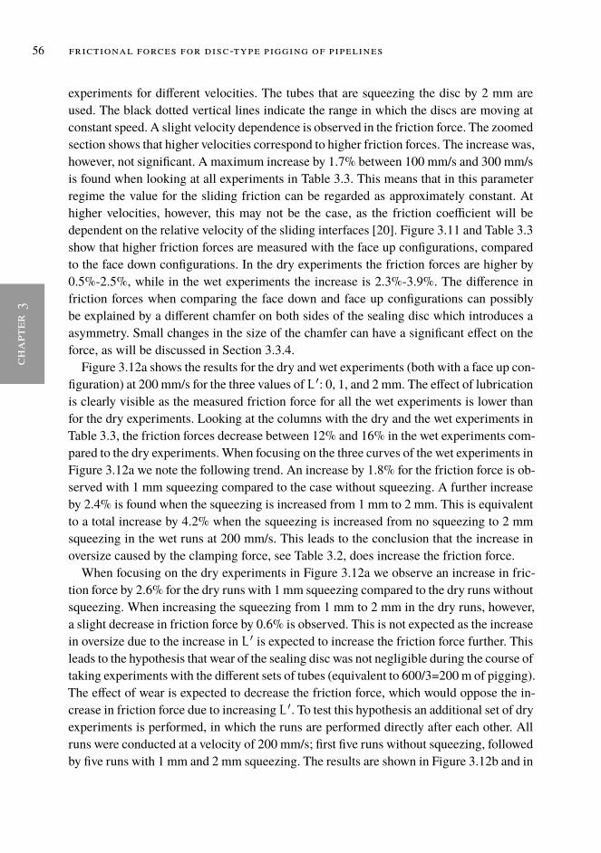
56 frictional forces for disc-type pigging of pipelines
chap
ter
3
experiments for different velocities. The tubes that are squeezing the disc by 2 mm areused. The black dotted vertical lines indicate the range in which the discs are moving atconstant speed. A slight velocity dependence is observed in the friction force. The zoomedsection shows that higher velocities correspond to higher friction forces. The increase was,however, not significant. A maximum increase by 1.7% between 100 mm/s and 300 mm/sis found when looking at all experiments in Table 3.3. This means that in this parameterregime the value for the sliding friction can be regarded as approximately constant. Athigher velocities, however, this may not be the case, as the friction coefficient will bedependent on the relative velocity of the sliding interfaces [20]. Figure 3.11 and Table 3.3show that higher friction forces are measured with the face up configurations, comparedto the face down configurations. In the dry experiments the friction forces are higher by0.5%-2.5%, while in the wet experiments the increase is 2.3%-3.9%. The difference infriction forces when comparing the face down and face up configurations can possiblybe explained by a different chamfer on both sides of the sealing disc which introduces aasymmetry. Small changes in the size of the chamfer can have a significant effect on theforce, as will be discussed in Section 3.3.4.
Figure 3.12a shows the results for the dry and wet experiments (both with a face up con-figuration) at 200 mm/s for the three values of L ′: 0, 1, and 2 mm. The effect of lubricationis clearly visible as the measured friction force for all the wet experiments is lower thanfor the dry experiments. Looking at the columns with the dry and the wet experiments inTable 3.3, the friction forces decrease between 12% and 16% in the wet experiments com-pared to the dry experiments. When focusing on the three curves of the wet experiments inFigure 3.12a we note the following trend. An increase by 1.8% for the friction force is ob-served with 1 mm squeezing compared to the case without squeezing. A further increaseby 2.4% is found when the squeezing is increased from 1 mm to 2 mm. This is equivalentto a total increase by 4.2% when the squeezing is increased from no squeezing to 2 mmsqueezing in the wet runs at 200 mm/s. This leads to the conclusion that the increase inoversize caused by the clamping force, see Table 3.2, does increase the friction force.When focusing on the dry experiments in Figure 3.12a we observe an increase in fric-
tion force by 2.6% for the dry runs with 1 mm squeezing compared to the dry runs withoutsqueezing. When increasing the squeezing from 1 mm to 2 mm in the dry runs, however,a slight decrease in friction force by 0.6% is observed. This is not expected as the increasein oversize due to the increase in L ′ is expected to increase the friction force further. Thisleads to the hypothesis that wear of the sealing disc was not negligible during the course oftaking experiments with the different sets of tubes (equivalent to 600/3=200m of pigging).The effect of wear is expected to decrease the friction force, which would oppose the in-crease in friction force due to increasing L ′. To test this hypothesis an additional set of dryexperiments is performed, in which the runs are performed directly after each other. Allruns were conducted at a velocity of 200 mm/s; first five runs without squeezing, followedby five runs with 1 mm and 2 mm squeezing. The results are shown in Figure 3.12b and in
[ January 15, 2020 at 7:46 – classicthesis version 2.2 ]

chapter3
3.3 results 57
Figure 3.12: (a) Friction force for three different pre-squeeze values and for two lubrication condi-tions. The pull velocity is 200 mm/s. (b) Friction force for three different pre-squeezevalues; the experiments have been conducted directly after each other. The pull veloc-ity is 200 mm/s.
Table 3.4. The inset in Figure 3.12b reveals the individual three time series on which thevalue in Table 3.4 is based. This shows excellent reproducibility for the subsequent runs.Indeed the friction force increases when the disc is squeezed. An increase by 1.6% isobserved with 1 mm squeezing compared to no squeezing and an increase by 1.7% for2 mm squeezing compared to 1 mm squeezing. Thus a total increase by 3.3% with 2mm squeezing compared to no squeezing. This confirms the hypothesis that wear is notnegligible during the course of taking experiments with the different sets of tubes. Wearcan only be approximately ignored when the runs are conducted directly after each other.Indeed, wear is clearly visible upon inspecting the sealing disc. In Figure 3.13 disc Ais shown before using it in the dynamic experiments and after all experiments were con-ducted. It can be seen that the disc is fabricated with a certain chamfer on both sides. After
[ January 15, 2020 at 7:46 – classicthesis version 2.2 ]

58 frictional forces for disc-type pigging of pipelines
chap
ter
3
Table 3.4: Dry runs performed with the three sets of tubes: 0 mm (no squeezing), 1 mm and 2mm. The mean values of the force data are tabulated, averaged over the five runs andas found when the disc is moving at a constant velocity of 200 mm/s. Every run isrepeated five times, corresponding to 50 m of pigging distance. Figure 3.12b shows allforce measurements.
L ′ [mm] Friction force [N]0 8131 8262 840
Figure 3.13: The chamfers of disc A are shown. Disc A on the left is not used in the dynamicexperiments and reveals the chamfer of approximately 1.4 mm as built-in by the man-ufacturer. On the right disc A is shown which is used in the dynamic experiments.The wear is clearly visible and the chamfer is 4 mm.
completing all experiments, which means that the disc was used over a distance of approx-imately 1500 m, the chamfer has increased significantly to a length of 4 mm. In the nextsection the results of the dynamic experiments will be related to the static experimentsas described in Section 3.3.2. The effect of the size chamfer in the translation from staticexperiments to the dynamic experiments will be discussed.
3.3.4 relation between static and dynamic results
In Section 3.3.2 we have seen that the FE model is able to capture the results obtainedin the static setup, using the E-moduli obtained in stress and strain tests without the useof any fitting parameters. It is however not possible to investigate the effect of a possibleliquid film between the disc and the pipe wall on the friction factor with this setup, sincethe experiment is static. In the dynamic experiment it is however possible to investigatethe presence of a liquid, as was shown in section 3.3.3. The next step is to relate the static
[ January 15, 2020 at 7:46 – classicthesis version 2.2 ]

chapter3
3.3 results 59
results to the dynamic experiments. Both experiments measure the friction force, althoughthe wall normal force cannot be measured in the dynamic experiments. We therefore needto deduce µ for the dynamic experiments, using the results from the static experiments.Figure 3.14 shows the FE prediction of µ for the dynamic experiments, using three
values of the chamfer length c. Here the results of the FE model are shown in a similarway as in Section 3.3.2, but now for an oversize of 4.04%. In the static experiments withdisc A the tubes were not yet used, but the circumference of the disc after clamping wasmeasured. This circumference corresponds exactly to the circumference of disc A whensqueezed by 2 mm in the dynamic experiments. Therefore this oversize was chosen, seeTable 3.2.
Figure 3.14: Prediction of the µ values in the dynamic experiment, using three values of the cham-fer length c. Using the FE results, the force data from the dynamic experiments aretranslated into µ values. µ is predicted between 0.97 and 1.30 in the dry runs andbetween 0.68 and 0.83 in the wet runs.
When averaging the friction force for the different speeds for the dry experiments withL ′ = 2 mm (Table 3.3), a value of 839 N is found. Based on this value a correspondingµ value can be determined using the FE model. Wear was observed during the course ofperforming the dynamic experiments and it was found to increase the chamfer length c,see Figure 3.13. To investigate the sensitivity of the chamfer size on the frictional force theFE calculations were performed with three different chamfer lengths: the original chamferlength c = 1.4mm, the final chamfer length c = 4mm, and an intermediate chamfer lengthc = 2.7 mm. It can be observed that the friction force decreases when the chamfer lengthincreases, as it is easier to subject the sealing disc to 4.04% oversize when the chamfer islarger. This is in line with other research and a consequence is that the required drivingpressure needed to propel the pig decreases throughout the course of a pigging run [98].When we focus on a fixed value of 839 N for the friction force in the dry experiments, wethus find differentµ values, ranging betweenµ = 0.97 andµ = 1.30. Thewet experimentscorrespond to lower friction values, see Section 3.3.3, and therefore lower corresponding
[ January 15, 2020 at 7:46 – classicthesis version 2.2 ]

60 frictional forces for disc-type pigging of pipelines
chap
ter
3
Table 3.5: Force ratio µ versus the chamfer length c.c [mm] µ [-], dry µ [-], wet1.4 0.97 0.682.7 1.11 0.754.0 1.30 0.83
µ values are found, see Figure 3.13. The results are summarized in Table 3.5. In the wetcontact µ decreases by approximately 30%. An interesting follow-up experiment could beto use a biological or mineral oil as lubricant in the dynamic pig pull experiments.
3.4 conclusions
A static and dynamic experimental setup have been designed to investigate the frictionalbehaviour of a sealing disc of a pipeline pig. The static setup has been used to systemati-cally study the effect of various parameters including the oversize, force ratio, thicknessand E-modulus. In this way the study contributes to the fundamental knowledge on pa-rameters influencing the friction force in pigging applications. Being able to test sealingdisc configurations for different values of the force ratio µ is important for the industry asµ is often unknown and may vary a quite substantially.
A finite element (FE) model was built which was able to accurately capture the be-haviour of the experiments. The finite element model was able to accurately describe thestatic experiments, by using E-moduli obtained in stress and strain tests and without usingany fitting parameters. When similar forces as measured in the experiment are acting onthe chamfer in the finite element model, the maximum deformation varies by less than 2mm for µ values larger than 0.25. Furthermore, the shapes obtained in the experimentsagree very well with the shapes obtained with the finite element model. In the currentexperiment and FE model axisymmetry applies. For future research it could be interest-ing to investigate the effect of gravity which would break the axisymmetry. This effect isexpected to become important when the gravitational forces become comparable with theforces which are purely caused by confining the sealing discs in the pipe.When the disc is brought to a specific oversize between 1% and 4% in the finite ele-
ment model, the required forces agree very well with the experimental force data. Themaximum deviations for disc A and B occurred at 4% oversize. Here the finite elementmodel underpredicts the friction force by a maximum of 5.2% and 11.6%, respectively. Itis hypothesized that this underprediction is explained by undesired friction between thehull and the frame in the experimental setup, which is especially observed at high frictionsforces. To test if this hypothesis is correct a setup could be designed which has more rollerbearings between the hull and the frame which would result in even less friction.
[ January 15, 2020 at 7:46 – classicthesis version 2.2 ]

chapter3
3.4 conclusions 61
The dynamic pig pull facility has been used to test the frictional behaviour during adynamic pull test through a 1.7 meter pipe for both a dry and a wet contact. This dynamicsetup is complementary to the static pig pull facility. The influence of the clamping forceof the spacer discs on the sealing disc diameter and frictional force has been investigated. Itwas found that by increasing the clamping force the diameter, and therefore the oversize, ofthe sealing disc increases. As a result the frictional force was found to increase during thedynamic pull tests. The largest difference in friction force is observed when comparing thedry and the wet experiments. Lubrication was clearly visible in the force measurements.Using water as a lubricant resulted in a decrease in the friction force by between 12%and 16% for the experiments conducted. This decrease in friction force is attributed toa difference in friction coefficient, which has been quantified using FE calculations. Thesensitivity of the size of the chamfer in this analysis has been taken into account. This hasled to a prediction of the friction coefficient of between 0.97 and 1.30 for a dry contact andof values between 0.68 and 0.83 for a wet contact. Only water has been used as lubricantin the experiments. It is suggested for future research to study also other lubricants, suchas for example mineral oil.
[ January 15, 2020 at 7:46 – classicthesis version 2.2 ]

[ January 15, 2020 at 7:46 – classicthesis version 2.2 ]

chapter4
4EXPER IMENTS AND MODELL ING OF BY- PASS P IGG INGUNDER LOW PRESSURE COND IT IONS
This chapter is adopted from M.H.W. Hendrix, H.P. IJsseldijk, W.-P. Breugem, and R.A.W.M. Henkes, "Ex-periments and modelling of by-pass pigging under low pressure conditions". In: Journal of Process Control71 (2018), pp. 1-13.
63
[ January 15, 2020 at 7:46 – classicthesis version 2.2 ]

64 experiments and modelling of by-pass pigging under low pressure conditions
chap
ter
4
4.1 introduction
Pipelines are used in many industries as a means of transporting fluids. Such fluids canconsist of gases, liquids, or combinations of gases, liquids and solids. An inevitable con-sequence is the internal maintenance of those pipelines. In the oil and gas industry this isdone by using a pig (Pipeline Inspection Gauge). This is a cylindrical device which travelsthrough the pipeline driven by the fluid flow, see for example figure 4.1. Pigs have a widerange of applicability, including cleaning the inside of a pipeline, removing excessive liq-uid from a liquid-gas pipeline, or distribution of corrosion inhibitor [15, 74, 94, 96]. Pigscan also be equipped with intelligent sensors which can inspect the inner pipe wall [75],for example. There is a wide variety of pigs to perform these tasks. An example of threecommon utility pigs are (1) the mandrel pig, (2) the solid cast pig and (3) the foam pig,which are shown in figure 4.1 [74]. A mandrel pig consists of a metal core with elementsmounted on this core. It depends on the purpose of the pigging operation which elementsare mounted. Typical elements are scrapers for cleaning, guiding discs to ensure a properalignment with the pipe and sealing elements to seal the pipe. These elements are nor-mally made from polyurethane. A solid cast pig differs from a mandrel pig in the sensethat it is made out of one material, often also polyurethane. A foam pig is made of softermaterial and has a larger volume. The pigging purpose and the costs determine which ofthe types is most appropriate to perform a pigging operation.
Figure 4.1: Several pig types: (a) Mandrel pig. (b) Solid cast pig. (c) Foam pig. (d) By-pass pig.Adapted from [74] and [53].
It is desirable that the product flow, which is driving the pigs through the pipeline, is in-terrupted as little as possible during the pigging operation. Conventional pigs, such as the
[ January 15, 2020 at 7:46 – classicthesis version 2.2 ]

chapter4
4.1 introduction 65
ones displayed in figure 4.1a-c, typically completely seal the pipeline. As a consequencethe speed of the device will be equal to the velocity of the product flow. However, oftena lower travel speed is desired, as a too high pig velocity may damage the pig or pipeline.In addition, it has been shown that a lower pig velocity is also beneficial for the cleaningand inspection performance of the pig [63, 96]. A solution to achieve a lower pig velocitywhile avoiding production deferment is the use of a by-pass pig, which does not seal thecomplete pipeline. Instead, a by-pass pig has a hole, or by-pass area, which allows fluid toby-pass the pig while it is moving inside the pipeline, see figure 4.1d. The presence of aby-pass will cause that the pig velocity is not dictated by the velocity of the product flow.Instead the pig velocity will be lower and it is now determined from a balance between thedriving pressure force and the friction force between the pig and the pipe wall [82]. Therisk, however, of using a by-pass pig is that the driving force on the pig becomes too low toovercome the wall friction force, which will result in a pig being stuck in the pipeline. Tomitigate the risk of a stuck pig, so-called speed controlled pigs have been designed whichhave an adjustable by-pass area which provides the right amount of by-pass such that thevelocity of the pig is lowered, while the pig does not get stuck [63]. Detailed mechanismson how such a control system should be designed are only scarcely found in literature [62,68].In this study we consider the movement of a pig in a low pressure gas-filled pipeline.
Pigging of such low pressure gas-filled pipelines in actual field operation can lead to largeoscillations in the pig velocity due to the compressibility of the gas, see for example [67,90]. This is because compressed gas pockets may build up at the upstream side of thepig when it is moving slower due to locally increased friction caused by for exampleirregularities in the inner pipe diameter. When the pressure in such a pocket has beensufficiently built-up, it is able to catapult the pig, resulting in large pig velocity excursions.This can lead to an unsafe and inefficient pigging operation. The effect described abovegets more pronounced when the operating pressure or the flow velocity in the pipe is low.It can even result in a so-called ‘stick-slip motion’, where the pig slows down completelyafter a period of high velocity. This stick-slipmotion of the pig is generally undesired in theindustry. However, when a pig is equipped with appropriate speed control, the occurrenceof high pig velocities in low pressure gas filled pipelinesmay be suppressed, which enablessafe and effective pigging of these pipelines.This chapter is built up as follows. In section 4.2 we first discuss the force balance on
a (by-pass) pig. In addition we derive a simplified model which describes the motion of apig in a low pressure system. The simplified model gives insights into the basic physicalmechanisms which are key to unsteady pig motion due to low pressure conditions in gasfilled pipelines. The simplified model relies on some assumptions, most notably the as-sumption that the pressure upstream of the pig is directly determined by the volume thatthe gas occupies upstream of the pig. In reality the pressure upstream of the pig will changeas result of a transient pressure wave, rather than a instantaneous response to the changein volume. We therefore also include a more complete approach which models the motion
[ January 15, 2020 at 7:46 – classicthesis version 2.2 ]

66 experiments and modelling of by-pass pigging under low pressure conditions
chap
ter
4
of the pig in a transient 1D pipe model. In section 4.3 we describe the experimental setupthat has been used to perform pigging experiments. The experimental setup has been usedin a previous work to test a prototype of a speed controlled pig [36, 44]. In this work wemore systematically study the behaviour of by-pass pigs with constant by-pass area which,in combination with the developed models, is expected to improve the design of such aspeed controlled pig. In section 4.4 a comparison will be made between the experimentalresults and the various models. The proposed models and experiments are subsequentlyused for the design of a PD controller in order to reduce pig velocity excursions throughdynamically adjusting the size of the by-pass. Section 4.5 gives conclusions and discussespossibilities for future research.
4.2 models
Whereas the pig velocity Upig of a conventional pig in a pipeline is dictated by the bulkvelocity U upstream of the pig, the pig velocity of a by-pass pig will be lower becausepart of the fluid is able to flow through the by-pass pig, see figure 4.2.
Figure 4.2: (a) Schematic motion of: (a) a conventional pig (b) a by-pass pig.
The motion of a by-pass pig in a horizontal pipeline is determined from a force balancebetween the driving pressure force Fp and frictional force Ffric. By applying a controlvolume analysis over the whole pig (including the by-pass area), Fp can be expressed asFp = ∆pA where ∆p is the pressure drop over the pig and A is the pipe cross-sectionalarea. The pressure drop is usually characterized by a pressure loss coefficient K definedas [45]:
K =∆p
12ρbpU
2bp
. (4.1)
Here ρbp is the density of the fluid in the by-pass (which is taken as the density down-stream of the pig) and Ubp is defined as the fluid velocity in the by-pass region takenrelative to the pig velocity, see [35, 82]. A mass balance taking into account a higher den-
[ January 15, 2020 at 7:46 – classicthesis version 2.2 ]

chapter4
4.2 models 67
sity upstream of the pig ρup due to compressibility of the fluid thus yields the followingexpression for Ubp:
Ubp =D2
d2ρup
ρbp(U−Upig). (4.2)
Here D is the pipe diameter and d the diameter of the by-pass hole. Substituting thisexpression for Ubp into equation 4.1 and applying a steady state force balance on the pig(∆pA = Ffric) results in an equation for the velocity of the by-pass pig [30, 82]:
Upig = U−d2
D2ρbp
ρup
√Ffric
K12ρbpA. (4.3)
When the by-pass area fraction d2/D2 goes to zero, equation 4.3 returns a pig velocityequal to the bulk velocity, as is the case for a conventional pig. When d2/D2 is not equalto zero, detailed knowledge of both K and Ffric are needed in order to accurately predictthe pig velocity. The pig geometry in this research can be regarded as a thick orifice, forwhich the following correlation for the pressure loss coefficient has been proposed byIdelchik [45]:
K = 0.5(1−
d2
D2
)0.75
+4fLpig
d+
(1−
d2
D2
)2. (4.4)
Here Lpig denotes the length of the pig, and f is the Fanning friction coefficient which hasbeen calculated using the Churchill correlation [13]. Equation 4.4 can be recognized as acombination of the loss associated with a sudden compression (first term), frictional lossin the by-pass (second term), and a sudden expansion (third term). This correlation hasbeen extensively verifiedwith simulations using CFD (Computational FluidDynamics) [5,82]. The loss coefficient for a by-pass pig that has a design different from a thick orificegeometry has been studied in [35]. Regarding the friction force Ffric, two main types offriction can be distinguished: (1) dry friction and (2) lubricated friction [72]. In case oflubricated friction (which obviously is only possible for twophase gas-liquid flow), a thinliquid layer is formed in between the two solids that is said to lubricate the relative motion.Such a lubrication layer normally reduces the friction coefficient considerably [84]. Ourexperiments are, however, carried out in a dry pipeline using air as working fluid. Wemodel the dry sliding friction between the pig and the pipe wall with a constant coefficient.The proposed models of K and Ffric will be compared with experimental results whichare described in section 4.3. With Fp and Ffric in place, the equation of motion of the pigfollows as:
md2sdt2
= Fp − Ffric. (4.5)
[ January 15, 2020 at 7:46 – classicthesis version 2.2 ]

68 experiments and modelling of by-pass pigging under low pressure conditions
chap
ter
4
Herem and s are the mass and the position of the pig, respectively.We will now describe a simplified model and a more complete numerical model to
describe the motion of a pig in a low pressure pipeline.
4.2.1 simplified model
The simplified model considers the motion of the pig by modelling Fp as the force thatresults from the pressure in the gas pockets on both sides of the pig. It is assumed thatthe pressure in these pockets is uniform and adapts instantaneously to any changes in thevolume that they occupy. The pressure upstream pup of the pig thus reads
pup =p∗
ρ∗ρup =
p∗
ρ∗Mtot
As=p∗
ρ∗M0 + Mt
As. (4.6)
Here the ideal gas law is used to relate the pressure in the upstream pocket to the up-stream density ρup, using p∗ = 101 kPa and ρ∗ = 1.2 kg/m3 as reference values forair. Furthermore,Mtot denotes the total mass in the upstream pocket,A is the pipe cross-sectional area, and s is the location of the pig as measured from the inlet. The total massMtot is a sum of the initial massM0 at t = 0 and the (constant) mass flux at the inlet Mmultiplied by the time t.
Figure 4.3: (a) Schematic motion of simplified pig model.
Applying the same approach to the downstream side of the pig leads to a constant pres-sure pdown = pout for the downstream gas pocket. This approach effectively neglectsfrictional pressure losses. Substituting Fp = A(pup − pdown) into equation 4.5 yields:
md2sdt2
=p∗
ρ∗M0 + Mt
s−Apout − Ffric. (4.7)
The equilibrium position s(t) = seq(t) can be found by setting the left hand side ofequation 4.7 equal to zero, which gives:
seq(t) =p∗
ρ∗M0 + Mt
Apout + Ffric. (4.8)
[ January 15, 2020 at 7:46 – classicthesis version 2.2 ]
chapter4
4.2 models 69
The equilibrium velocity veq can be found by differentiating equation 4.8, which yields:
veq =p∗
ρ∗M
Apout + Ffric. (4.9)
We now define s(t) = seq(t) + δs(t). Dividing equation 4.7 by Apout + Ffric andsubstituting the decomposition of s into equation 4.7 yields
m
Apout + Ffric
d2δsdt2
=seq(t)
seq(t) + δs− 1. (4.10)
Assuming that the perturbations of δs are small (δs seq) we can expand the first termon the right hand side of equation 4.10:
m
Apout + Ffric
d2δsdt2
= −δs
seq(t). (4.11)
Equation 4.11 can be solved analytically (see Appendix C), yielding an explicit expressionfor δs(t):
δs(t) = C1kJ1(2k) −C2kY1(2k). (4.12)
Here J1 is the Bessel function of the first kind with order 1 and Y1 is the Bessel functionof the second kind with order 1. Futhermore k(t) is given by:
k(t) = ω(t)
(M0
M+ t
), (4.13)
whereω(t) is given by:
ω(t) =
√(Apout + Ffric)
seq(t)m. (4.14)
Differentiating equation 4.12 yields an expression for the perturbed velocity δv (see Ap-pendix C):
δv(t) = ω2(t)
(M0
M+ t
)(C1J0(2k) −C2Y0(2k)) . (4.15)
C1 andC2 are integration constants (with unit length) which can be found from the initialconditions for δs and δv. This approximate analytic expression will be compared withnumerical integration of equation 4.7 in section 4.4.3.
[ January 15, 2020 at 7:46 – classicthesis version 2.2 ]
70 experiments and modelling of by-pass pigging under low pressure conditions
chap
ter
4
4.2.1.1 Local analysis
When fixating the value for seq, Equation 4.11 can be recognized as the equation whichdescribes a harmonic oscillator, for which the solution is given as:
δs(t) = C3 sin(ωt+C4). (4.16)
Here ω is the local frequency of the solution for a given seq, as given by equation 4.14,and C3 and C4 are integration constants. The maximum value for δvmax can be foundby differentiating Equation 4.16 and determining the maximum which gives:
δvmax = C3ω. (4.17)
The value ofC3 (andC4) is determined by the initial conditions for δs(t = 0) and δv(t =0), which we denote δs0 and δv0 respectively. C3 can then be determined as:
C3 =
√ω2δs20 + δv
20
ω. (4.18)
Substituting this expression for C3 into equation 4.17 gives:
δvmax =
√ω2δs20 + δv
20 =
√Apout + Ffric
seqmδs20 + δv
20. (4.19)
In order to determine δs0 and δv0 and seq we now consider a pig which moves in a stick-slip fashion and just enters the slip phase. In this analysis we introduce the static frictionforce Ffric,s, which is usually higher than the value of the sliding dynamic friction forceFfric. We now consider a pig that sticks at a location L = seq + δs0. Just at the pointbefore the pig starts slipping (t = 0) a force balance can be constructed which reads:
(pup − pout)A =
(p∗
ρ∗M0
AL− pout
)A = Ffric,s (4.20)
This equation can be solved forM0 and the result can be substituted into Equation 4.8 toyield an expression for the equilibrium position seq:
seq =L(Ffric,s + PoutA)
Ffric + PoutA. (4.21)
[ January 15, 2020 at 7:46 – classicthesis version 2.2 ]

chapter4
4.2 models 71
Using δs0 = L − seq and δv0 = −veq and substituting these expressions into Equa-tion 4.19 gives the following expression for the maximum velocity vmax which occursduring the stick-slip cycle:
vmax = veq + δvmax = veq +
√L(Ffric,s − Ffric)2
m(Ffric,s + PoutA)+ v2eq. (4.22)
We note that if the static friction force Ffric,s equals the dynamic friction force Ffric themaximum velocity is simply equal to twice the upstream equilibrium velocity veq.
4.2.2 full numerical model
The full numerical model discretizes the fluid domain into multiple finite volumes, ratherthan describing the fluid upstream and downstream of the pig as one pocket as was donein the model described in section 4.2.1. The resulting model is a one-dimensional (1D)transient model, which solves for cross-sectionally averaged quantities such as pressureand velocity as function of the pipe coordinate s, which runs along the pipe, and time t.Examples of 1D transient tools which are used in the oil and gas industry to model pigmotion in a pipeline include OLGA and LedaFlow [8, 28]. The current 1D model relieson the 1D extended Euler equations from which the cross-sectionally averaged mass andmomentum equation read:
∂
∂t(ρA) +
∂
∂s(ρuA) = 0, (4.23)
∂
∂t(ρuA) +
∂
∂s(ρu2A+ pA) = −τ(πD). (4.24)
Here τ is the wall shear stress which is calculated as:
τ =1
2ρu2f, (4.25)
where f is the Fanning friction coefficient calculated using the Churchill relation [13].As in the simplified model, we calculate ρ = ρ(p) through the ideal gas law, that isρ = (ρ∗/p∗)p. Equations 4.23 and 4.24 form a closed system of equations which isdiscretized using the finite volume method on a staggered grid, see figure 4.4.Conservation of mass (equation 4.23) is discretized on the p-volume Ωp, in which p isdefined at the center of the volume:
ddt(ρiΩ
pi
)+ ρi+1/2ui+1/2A− ρi−1/2ui−1/2A = 0 (4.26)
[ January 15, 2020 at 7:46 – classicthesis version 2.2 ]
72 experiments and modelling of by-pass pigging under low pressure conditions
chap
ter
4
Figure 4.4: Staggered grid layout in the full numerical model.
HereΩpi = A∆si = A(si+1/2− si−1/2) is the size of the finite p-volume. Conservationof momentum (equation 4.24) is discretized in a similar way:
ddt
(ρi+1/2ui+1/2Ω
ui+1/2
)+ρi+1(ui+1)
2A−ρi(ui)2A = −τi+1/2(πD)∆si+1/2
(4.27)
Here Ωui+1/2 = A∆si+1/2 = A(si+1 − si) is the size of the finite u-volume. Someterms in equation 4.26 and 4.27 require interpolation. If the term is part of a convectiveterm a flux limiter is used, otherwise central interpolation is used. The system is inte-grated in time using the second order BDF2 scheme. For more details on the numericalimplementation, the reader is referred to chapter 6.
4.3 experimental setup
A schematic of the flow loop in which the laboratory experiments are conducted is de-picted in figure 4.5a. The loop consists of a horizontal transparent perspex pipe with alength of 62 meter and an internal diameter of 52 millimeter. The experiment is operatedin single phase using air as working fluid. The flow loop is equipped with a pig launcherlocated at the inlet of the loop that allows to insert a pig into the system, see figure 4.5b. Byplacing the pig in the launcher and subsequently redirecting the air through the launcherthe pig will be inserted into the pipe. After traversing along the pipe the pig is trapped atthe outlet and can be retrieved. Figure 4.5c shows a close-up of one of the pigs that is usedin the experiments.The air that is used as working fluid in the experiment is tapped from an air supply
system which is kept at a pressure of 8 bar. A pressure reducing valve brings this down to
[ January 15, 2020 at 7:46 – classicthesis version 2.2 ]

chapter4
4.3 experimental setup 73
Figure 4.5: (a) Overview of the flow loop. (b) Close-up of the pig launcher. (c) Drawing of the pig.
2 bar. The air then passes through a gas flowmeter (Bronkhorst - MASS-STREAM SeriesD-6300) where the air mass flux can be controlled. The flow loop is equipped with twopressure sensors (Validyne DP15), see figure 4.5a. The average pig velocity is computedas the total length divided by the residence time. For the length, the distance between theupstream pressure transducer and the pig receiver (i.e. the flow loop exit) is used, whichamounts a distance of 62m. The residence time is the time difference found by studying thepressure increase and decrease measured by the upstream pressure transducer. In addition,the pressure drop that is measured over the pig allows to determine the frictional force ofthe pig with the pipe wall, since in steady state the driving pressure force and the frictionalforce must balance, see equation 4.5. Three synchronized high speed cameras (GoProHERO4) located at about 41.5 meter downstream of the first pressure sensor allow for thelocal dynamics of the pig to be analyzed, see figure 4.5a. The cameras are operated at aframerate of 120 frames per second at a resolution of 720p. The cameras are separatedin such a way that their field of views partly overlap. The three images of each cameraare stitched together during post-processing using a cross-correlation algorithm in orderto construct one single image. The total field of view thus obtained is 7.5 meter. Thecameras are synchronized in time by using a flash light as reference point which is visibleon all three cameras at the beginning of a measurement.
The pigs are custom-made and have a flexible modular design which allows for the by-pass area and sealing disks to be easily interchanged. The sealing disk makes sure that nofluid leaks between the pig and the pipe wall, and that the only fluid that flows throughthe pig goes through the by-pass area, see figure 4.5c. The by-pass area is formed by aconcentric hole in the centre of the pig body and ranges from 0% to 4% of the total cross-sectional area in the current experiment.
[ January 15, 2020 at 7:46 – classicthesis version 2.2 ]
74 experiments and modelling of by-pass pigging under low pressure conditions
chap
ter
4
Two pig configurations have been tested: configuration 1 and configuration 2, see fig-ure 4.6a and figure 4.6b respectively. Both configurations have a sealing disk with aslightly larger diameter than the inner pipe diameter. The difference in the diameters, orthe oversize, ensures that the pig properly seals the pipeline and that no leakage occursbetween the pig and the pipe wall [74].
Figure 4.6: (a) Schematic of pig configuration 1. (b) Schematic of pig configuration 2. (c) Detailedgeometry of pig configuration 1. (d) Detailed geometry of pig configuration 2.
The two pig configurations have a different sealing disk compression behaviour. Theseals in configuration 1 are compressed in the radial direction. For industrial pigs, seal-ing disks deformed in a similar way are referred to as scraper disks [74]. Since the usedmaterial of our small-scale pigs is rather flexible, the variation in friction due to diametervariations is limited. Furthermore, the clamping disks can be relatively large which pre-vents tilting of the pig. A downside of the flexible seals is that severe wear of the sealingdisks can occur. In the current experiment they were therefore replaced after roughly every6 runs. The seals in configuration 2 have more space to bend compared to configuration1. This is comparable with what in industry is referred to as cone disks [74]. The sealingdisk material of configuration 2 is much harder and shows very good wear properties. Adownside is that more space is required for the seals to bend, which increases the chance
[ January 15, 2020 at 7:46 – classicthesis version 2.2 ]

chapter4
4.4 results 75
that the pig is being tilted. The dimensions of pig configurations 1 and 2 are displayed infigure 4.6c and in figure 4.6d, respectively. More details on the material and sizes of thesealing disks are listed in table 4.1. To build up sufficient pressure, it is essential that thepig properly seals the pipe. Cell rubber (EPDM) with a closed cell structure is chosen forconfiguration 1 to guarantee that the sealing disk is impermeable. Para rubber is used forconfiguration 2, which has very good wear properties.
Table 4.1: Properties of pig configurations.
Property Configuration 1 Configuration 2 UnitMaterial sealing disk 1 EPDM Para rubber -Hardness sealing disk 1 35 * 45 Shore A
Outer diameter sealing disk 1 57 57 mm
Thickness sealing disk 1 4 2 mm
Material sealing disk 2 EPDM EPDM -Hardness sealing disk 2 35 35 Shore
Outer diameter sealing disk 2 55 48 mm
Thickness sealing disk 2 4 4 mm
Average friction 25.68 41.3 N* The hardness is measured according Shore 00 standards. A comparable Shore A value is givenhere to compare with the other material
From the pressure measurements during the pigging runs an estimation of the frictionwas obtained for both configurations, see table 4.2. This table will be explained in moredetail in the next section.
4.4 results
This section starts with some overall results from the various pigging runs that have beenconducted in the lab facility. In total 72 runs were used in the analysis of configuration1, and 60 runs were performed with configuration 2. The overall quantities include theaverage pig velocity and the required driving pressure for various by-pass pigs. Theseresults are important for verifying steady state by-pass pigging models which can be usedto predict the pig velocity. In addition, the results are relevant for 1D transient models inwhich the trajectory of the pig can be monitored [8, 28]. These 1D transient models rely onaccurate correlations to model the pig dynamics. Subsequently, section 4.4.2 presents ananalysis of the local pig dynamics which gives insight in the oscillatory behaviour of thepig motion due to the low pressure conditions. A comparison with the models developed
[ January 15, 2020 at 7:46 – classicthesis version 2.2 ]

76 experiments and modelling of by-pass pigging under low pressure conditions
chap
ter
4
in section 4.2 will be made. The results for the local behaviour of the pig motion are usedin section 4.4.3 to design a simple PD controller to reduce the velocity excursions of thepig by dynamically adjusting the by-pass area.
4.4.1 overall behaviour
For each pigging run the pressure from the upstream and downstream pressure sensors isrecorded. Figure 4.7a shows a typical signal that is obtained. Here the mass inflow rateis M = 0.0089 kg/s, and the pig has configuration 2 with 0% by-pass. When the pigtraverses along the upstream pressure sensor the excess pressure increases to about 20kPa. After traversing 41.5 meter the pig reaches the downstream pressure sensor, whichis clearly visible by the uptake of the signal at around 16 seconds. When the pig reachesthe outlet of the pipe both signals drop because the pressure that was built up behind thepig is now released.
Figure 4.7: (a) Pressure signal for configuration 2 with 0% by-pass. (b) Average driving pressuresfor the configuration 1 pigging runs. (c) Average driving pressures for the configuration2 pigging runs. The symbols in (b) and (c) denote various by-pass ratios.
[ January 15, 2020 at 7:46 – classicthesis version 2.2 ]

chapter4
4.4 results 77
From the time difference between the instant that the pig reaches the upstream pressuresensor and the outlet, the average pig velocity can be obtained. In addition, the averagedriving pressure force needed to propel the pig can be deduced from the measurements,which in steady state balances the friction force between the pig and the pipe wall. Fig-ure 4.7b and 4.7c show the average driving pressures (pup − pdown) as function of thepig velocity for configuration 1 and for configuration 2, respectively. The measurementcorresponding to the pressure signal displayed in figure 4.7a is indicated by the black ar-row in figure 4.7c. The different pig velocities have been obtained by varying both theupstream bulk velocity of the air as well as the by-pass area, as will be explained in moredetail below. When inspecting figures 4.7b and 4.7c, we note that the driving pressureis not a function of the pig velocity. This substantiates our earlier modeling assumptionthat the friction of the pig can indeed be approximated by a constant (dry) friction forcewithin the current parameter range. It is important to note that this can be different whenthe transported fluid is a liquid instead of a gas or when there is two-phase gas-liquid flow,due to the effect of possible lubrication. From the data presented in figure 4.7 the overallaverage friction force for each by-pass pig (0,1,2, and 4%) for the two configurations canbe obtained. These average friction values, with the standard deviation, are summarizedin table 4.2. As can be noted from both figure 4.7 and table 4.2 no runs for a by-pass of4% were performed for configuration 2. The reason is that the friction of this pig with 4%by-pass is too high which results in a stalled pig.
Table 4.2: Properties of pig configurations.
By-pass area ratio(%)0 1 2 4
Configuration 1Average friction (N) 27.1 ± 6.5 25.5 ± 3.0 23.9 ± 5.0 26.5 ± 4.5Configuration 2Average friction (N) 40.3 ± 1.5 44.4 ± 2.9 39.5 ± 2.5 NA
One of the main reasons for using by-pass pigs is the ability to reduce the pig velocity. Theflow velocity can be kept at the nominal production rate whereas the pig travels throughthe pipeline at a lower velocity. The reduction in the pig velocity depends on the by-passratio, see equation 4.3. Figure 4.8 shows the pig velocity versus the flow velocity for bothconfigurations 1 and 2. Different colours and symbols are used for different by-pass arearatios.The red circles represent the pigging runs with zero by-pass. These pig velocities shouldbe equal to the upstream bulk velocity, which is indicated by the 45 degree line in gray.The results for both configurations indeed follow this line. The other markers representthe pig velocity for a specific by-pass ratio. As can be noted an increase in by-pass area
[ January 15, 2020 at 7:46 – classicthesis version 2.2 ]

78 experiments and modelling of by-pass pigging under low pressure conditions
chap
ter
4
Figure 4.8: Pig velocity as function of upstream bulk velocity (a) Configuration 1, (b) Configura-tion 2. The dashed lines denote the standard deviation in the calculated pig velocity.
does indeed result in a reduction of the pig velocity. It can be deducted from figure 4.8that the reduction in pig velocity is around 1 m/s for each percentage of by-pass area thatis added relative to the zero by-pass case. For a more quantitative comparison with theorywe compare the experimental results with the velocity predicted by equation 4.3, whichis shown by the black line. In this equation the friction force Ffric is taken equal to theaverage measured value of the friction, see table 4.2. The value for K in equation 4.3 ismodeled by the Idelchik relation (equation 4.4) to model the pressure drop. Therefore thesolid line effectively plots the predicted travel velocity based on the Idelchik relation anda constant predetermined friction. In addition the velocity calculated based on plus andminus the standard deviation of the friction force are included as black dashed lines. Aswas already shown in table 4.2, the spread is higher for configuration 1. Figure 4.8 showsvery good agreement between the measurements and the values based on the Idelchikrelation. During the pigging runs oscillatory motion of the pig was observed, which willbe discussed in the next section. These results show that even though equation 4.3 is basedon a steady state balance it can be applied to unsteady pig motion from which an averagepig velocity is extracted.We further note that the point where the black line intersects the horizontal axis indi-
cates a minimum average bulk velocity which is needed to propel the by-pass pig. Belowthis bulk velocity not enough driving pressure is generated to overcome the average fric-tion force of the pig with the pipe wall. Note that in practice the minimum required bulkvelocity may be higher as the black line is based on an average friction. A local increasein friction, for example due to irregularities in the pipe diameter, may cause a pig to stall
[ January 15, 2020 at 7:46 – classicthesis version 2.2 ]

chapter4
4.4 results 79
even above this velocity. In the next section we will discuss the local behaviour which isobserved by analyzing detailed dynamics of the pig motion as well as time series of theupstream pressure.
4.4.2 local behaviour
We now focus on the local behaviour of the pig motion. As was mentioned in the previoussection stick-slip motion was observed in the experiment. The oscillatory signal of thepressure (figure 4.7a) indicates that the pressure upstream of the pig is indeed not con-stant as would be expected in case the pig would move at a constant steady state velocity.Figure 4.9 shows the upstream pressure signal which is displayed in figure 4.7a togetherwith a prediction from the simplified model, as described in section 4.2.1. The model isinitiated at two time instances: t1 = 3.04 and t2 = 12.20 seconds. These instances areselected as case examples in the time series of the upstream pressure, as a clear oscillatorysignal is visible, see figure 4.9. In order to evaluate the simplified model to predict the up-stream pressure, equation 4.6 is used. To evaluate equation 4.6 the initial position of thepig needs to be known. Clearly, the pig is located further downstream at t = t2 than att = t1. To determine the initial pig positions for these two cases, the equilibrium velocity(Equation 4.9) is multiplied by the traveling time t1 and t2. Furthermore, the dynamicfriction force Ffric and the static friction force Ffric,s are input parameters to the model.Ffric has been estimated by determining the mean driving pressure which is needed topropel the pig multiplied by the pipe area, as has been described in 4.4.1. Ffric,s is esti-mated at 1.5 times the standard deviation of the pressure signal of the upstream pressuresensor multiplied by the pipe area. This leads to Ffric = 40.80 N and Ffric,s = 43.87 N.The pressure values which are needed to balance the friction forces Ffric and Ffric,s areindicated with a dashed and a dotted line respectively, see figure 4.9.
0 5 10 15 20 25
Time [s]
0
1
2
3
Pre
ssure
[P
a]
104
Pressure sensor (upstream)
Simplified model
Figure 4.9: Pressure signal for configuration 2 with 0% by-pass compared with the simplifiedmodel. The horizontal dashed lines represent the average pressure plus and minus 1.5times the standard deviation of the pressure multiplied by the pipe area.
[ January 15, 2020 at 7:46 – classicthesis version 2.2 ]

80 experiments and modelling of by-pass pigging under low pressure conditions
chap
ter
4
Figure 4.9 shows qualitatively good agreement between the measured upstream pressureand the value obtained with the simplified model. Both the model and the measurementsshow that the frequency of the oscillation decreases when the pig moves further throughthe pipeline. This is in line with equation 4.14, which describes the local frequency of theoscillation. It must be noted that the simplified model idealizes the model of the frictionin the sense that it assumes one value of the static friction Ffric,s and one value of thedynamic friction Ffric. In reality the value of Ffric,s may vary due to for example irreg-ularities in the inner pipe diameter. Nonetheless it can be observed that the frequency ofoscillations of the pig motion can be captured by the model by estimating constant valuesfor Ffric and Ffric,s.The oscillation in pressure which was discussed above is directly connected to oscilla-
tions in the pig velocity. We now use the images from the high speed cameras, which arelocated around 41.5 meter downstream of the upstream pressure sensor (see figure 4.5),to investigate the maximum pig velocity that occurs. The maximum velocity is foundfrom the video recordings by tracking the location of the pig using image processing, asdiscussed in section 4.3. The experiments performed with configuration 2 are selected,because the spread in average friction is smaller compared to configuration 1, see sec-tion 4.4.1. The results are shown in figure 4.10a. The coloured symbols represent thedifferent by-pass pigs that are used in the experiment. In addition the maximum velocityas predicted by the simplified model, equation 4.22, is shown. Here the dynamic frictionFfric is taken equal to the value of the 0% by-pass pig, which is 40.3 N, see table 4.2.The static friction Ffric,s is taken equal to 40.3 N, 44 N, and 48 N, as shown by the solid,dashed, and dotted line, respectively. It is clear from figure 4.10a that a higher value ofFfric,s promotes a higher maximum pig velocity. This is explained by the higher pres-sure in the gas pocket upstream of the pig corresponding to the higher value of the staticfriction force Ffric,s. The black solid line represents the maximum pig velocity in caseFfric,s is equal to Ffric. According to equation 4.22 this corresponds to a maximum pigvelocity which is twice the average pig velocity. From the measurements it is clear thatthe maximum pig velocity is indeed significantly higher than the average travel velocityof the pig as most of the measurements are located at the left of the solid line. In additionto the measurements and the simplified model, the results of the full numerical modelas explained in section 4.2.2 are included for the three different values of Ffric,s (lineswith solid black circles). The by-pass in this simulation is set equal to 0%. The maximumpig velocity has been obtained from a simulation in which the pig is inserted 40 meterdownstream. This location ensures that the maximum velocity occurs within the locationcorresponding to the field of view of the cameras in the experiment. Grid converged solu-tions were typically obtained when using a total of 200 finite volumes, which correspondsto a computational cell length of about 0.34 meter, and a timestep of 0.0025 seconds.When comparing the results of the simplified model with the full numerical model and
the experimental data we note that the simplified model overpredicts the maximum veloc-ity. This is due to the assumption in the simplified model that the influence of pressure
[ January 15, 2020 at 7:46 – classicthesis version 2.2 ]

chapter4
4.4 results 81
Figure 4.10: Maximum pig velocity versus average pig velocity: (a) Experimental conditions (b)Higher friction (10 times) compared to experimental conditions.
[ January 15, 2020 at 7:46 – classicthesis version 2.2 ]

82 experiments and modelling of by-pass pigging under low pressure conditions
chap
ter
4
waves due to the acceleration of the fluid around the pig are negligible. The full numericalmodel does incorparate this, and therefore predicts a lower maximum velocity within thisparameter range. The effect of these pressure waves compared to the overall pressure dropover the pig becomes less important if the friction force of the pig is larger. To test thishypothesis we run the same simulation, but now increase the value of Ffric by a factor10 to Ffric = 403 N. Again three values of Ffric,s have been chosen as 403 N, 422 N,and 440 N. We also increased the pig mass by a factor 10. We now see that the agreementbetween the simplified model and the full numerical model is much closer. Therefore weconclude that the simplified model can be used to estimate the maximum velocity if themagnitude of the pressure waves that occur in the fluid due to the acceleration of the pigare negligible compared to the pressure drop over the pig.Figure 4.10a shows the simplified model (lines) and the full numerical model (lines
with solid black circles) evaluated for the 0% by-pass case. The experimental results per-formed with the 1% and 2% by-pass pigs are superimposed in the plot. Although the travelvelocity of the by-pass pigs is lower, it can be noted that the results with 1% and 2% by-pass follow the trend of the results with 0% by-pass and thus have a significantly highermaximum velocity than the average travel velocity. We also have evaluated the simplifiedmodel by incorporating a by-pass. To make the simplified model suitable for by-pass pigs,equation 4.7 is modified to take into account the mass leakage that occurs through theby-pass:
md2sdt2
=p∗
ρ∗M0 + Mt−
∫Mβdt
s−Apout − Ffric, (4.28)
where Mβ is the mass flux through the by-pass given by
Mβ = (U−Upig)Aρup. (4.29)
Here U can be solved from equation 4.3 for a given mean pig velocity Upig. Instead ofconstructing an analytical solution, which was possible for 0% by-pass case, equation 4.28is solved numerically. As an example the results for Ffric,s = 48 N are included in fig-ure 4.10a with with white squares and white triangles for 1% and 2% by-pass respectively.These symbols closely follow the line of the simplified model corresponding to 0% by-pass. It can thus be concluded that a fixed by-pass area does not reduce the velocity excur-sion of the pig. This is also confirmed by the experimental results as shown in figure 4.10:although the average speed of the by-pass pigs is lower, the maximum velocity is still sig-nificantly higher than the average pig velocity. However when the by-pass area is not fixed,but instead is adjusted dynamically, the maximum pig velocity can be reduced, which willbe discussed in the next section.
[ January 15, 2020 at 7:46 – classicthesis version 2.2 ]
chapter4
4.4 results 83
4.4.3 control
In the previous sections themechanism behind oscillatorymotion of a pig in a low pressurepipeline has been explained and described. Due to stick-slip behaviour it was found thatthe maximum pig velocity is significantly higher than the average pig velocity for bothconventional pigs (i.e. no by-pass) as well as pigs with by-pass. We now propose a controlmechanism which relies on actively regulating the size of the by-pass, such that part of thepressure in the gas pocket upstream of the pig can be released. This would result in a lowermaximum pig velocity, as the driving upstream pressure is reduced during the accelerationof the pig. It is important to note that if the by-pass stays open too short or too little, notenough pressure is released and the pig still accelerates to a high velocity. On the otherhand, if the by-pass stays opens too long, too much pressure is released and instead ofmitigating the spike in pig velocity, a new stick-slip cycle is promoted. The ideal by-passopening can be determined by an appropriate control algorithm. The time scale on whichthe controller should act is given by 2π/ω, whereω is the local angular frequency of theoscillation, given by equation 4.14. We will now demonstrate a simple controller based onthe physical models that have been formulated, which set some minimum requirementsfor the design of a controller. Therefore we again consider a pig that sticks at location Lat t = 0. When defining s = s− L and v = ds/dt we can write equation 4.28 as:
md2sdt2
=p∗
ρ∗M0 +Mu
s+ L−Apout − Ffric. (4.30)
HereMu =∫t0(M− Mβ)dt is the upstreammass that has been added after the pig starts
moving. We can put equation 4.30 in state space form by selectingMu as control variableand linearizing around the point s = 0, v = 0,Mu = 0:
[˙s˙v
]=
[0 1
− p∗M0
ρ∗L2m0
][s
v
]+
[0p∗
ρ∗Lm
]Mu =
[0 1
−ω2 0
][s
v
]+
[0
veqω2
M
]Mu
(4.31)
v =[0 1
] [sv
]. (4.32)
In the final step in obtaining equation 4.31 above we assumed for simplicity, without lossof generality, that Ffric,s = Ffric. The corresponding transfer function P(σ) of the statespace model reads:
P(σ) =σveqω
2
M
σ2 +ω2. (4.33)
[ January 15, 2020 at 7:46 – classicthesis version 2.2 ]
84 experiments and modelling of by-pass pigging under low pressure conditions
chap
ter
4
Here σ denotes the complex frequency variable. A feedback loop with a linear controllerC(σ) may be constructed as shown in figure 4.11a.
Figure 4.11: (a) Feedback loop (b) Equivalent feedback loop with closed loop transfer functionT(σ).
The goal is to have no excursion in the pig velocity, and prefably it is equal or close toa preset reference velocity vref. Perhaps the simplest controller which would meet theserequirements is a PD-controller:
C(σ) = Kp +Kdσ (4.34)
The closed loop transfer function T as displayed in the equivalent blockdiagram in fig-ure 4.11b then follows as:
T(σ) =
veqω2
M
σ2 +ω2 +veqω2
M(Kp +Kdσ)
(4.35)
We now again consider the example case which has been discussed in section 4.4.2. Forthis case we have M = 0.0089 kg/s and Ffric = 40.80 N. This yields a value of veq =
2.94 m/s and ω = 6.21 rad/s, see equation 4.9 and equation 4.14 respectively. The openloop response of the linear system to a mass influx M at t = 0 is marginally stableand is shown by the black line in figure 4.12a. Indeed when performing the numericalintegration of equation 4.30 the pig velocity shows persisting oscillations, as shown bythe red squares in figure 4.12a. We note that these numerical results for the 0% by-passcase are well captured by using the analytical approximation of equation 4.15, as shownby the red solid line. We now focus on damping the oscillation. The damping ratio of thesecond order system (equation 4.35) can be identified as:
ζ =
veqω2
MKd
2
√ω2 +
veqω2
MKp
. (4.36)
[ January 15, 2020 at 7:46 – classicthesis version 2.2 ]

chapter4
4.4 results 85
Furthermore, we note that a constraint on the controller is that Mβ has a maximum equalto M. The typical error in the velocity e can be estimated as −veq, which is equal to theerror in the beginning of a slip phase, as the actual pig velocity is still zero at that point. Ina similar fashion, we estimate de/dt as 2veqω/π, which is the average acceleration from0 to 2veq in the time period π/ω. Using these estimations of e and de/dt the followingrequirement can then be formulated:
Kpe+Kddedt
= −Kpveq +Kd2veq
πω= M. (4.37)
Kp and Kd can now be solved from equation 4.36 and equation 4.37 and expressed as:
Kp =M(16ζ2 − π2)
veqπ2kg/m (4.38)
Kd =M8ζ2
veqωπkg s/m. (4.39)
Oscillations will be damped when ζ > 1. We choose a value of ζ = 1.2, which yieldsKp = 0.0041 kg/m and Kd = 0.0018 kg s/m. The result of this closed loop system isshown in figure 4.12c/d. The linear response of the closed loop system (black solid line),as well as numerical integration (red squares) indeed show that the pig velocity does notovershoot but now approaches the reference velocity (dashed black line), which has beenset just below veq at a value equal to 2.75m/s. In order to obtain this pig velocity trajectory,Mβ and the corresponding by-pass opening have been increased for a short time period torelease the excess pressure of the upstream gas pocket. This is shown by the black trianglesin figure 4.12d and the blue triangles in figure 4.12c respectively.The simplified model relies on various assumptions, most notably the assumption thatthe pressure in the gas pocket upstream and downstream of the pig is instantaneouslydetermined by the volume that the gas pocket occupies. The 1D full numerical modelas described in section 4.2.2, however, contains more physics and does not rely on thisassumption. We now apply the controller derived from the simplified model directly onthe full numerical model. The result is shown by the black circles in figure 4.12c. Althoughsome oscillations are still present, the maximum pig velocity also in this case is clearlydiminished. In very long pipelines the assumption of an instantaneous pressure responsein the simplified model will not hold. It is therefore recommended for future research tofurther investigate the applicability of the simplified model in long pipelines. Instead ofselecting the upstream massMu as a control parameter, a local pressure analysis aroundthe pig may be more appropriate in this case.The above example illustrates some minimum requirements on a controller which can
be used to reduce pig velocity excursions in low pressure pipelines. In order to realizethis in practice, the pig needs to be able to track at least the following quantities: pig
[ January 15, 2020 at 7:46 – classicthesis version 2.2 ]

86 experiments and modelling of by-pass pigging under low pressure conditions
chap
ter
4
Figure 4.12: (a) Pig velocity and by-pass opening without control. (b) Mass flow rate without con-trol. (c) Pig velocity and by-pass opening with control. (d) Pig velocity and by-passopening with control.
velocity, pig acceleration, and the pressure upstream of the pig. Clearly the pig velocityneeds to bemeasured in order to evaluate the error e compared to a preset desired referencevelocity. The pig velocity is usually measured by odometer wheels attached to the pigwhich touch the inner pipe wall and thereby record the velocity, see for example [63]. Theacceleration needs to be measured to evaluate de/dt to anticipate on a possible velocityexcursion of the pig as soon as it starts moving. The acceleration can be measured with anaccelerometer.Measurement of the upstream pressure will help to determineM0, which isespecially relevant when the local static friction Ffric,s is larger than the dynamic frictionFfric.
[ January 15, 2020 at 7:46 – classicthesis version 2.2 ]

chapter4
4.5 conclusions 87
4.5 conclusions
The motion of by-pass pigs in a horizontal low pressure gas pipeline has been studied ona laboratory scale. The effect of the by-pass area and of the upstream bulk velocity wasanalyzed by means of an extensive experimental parameter study.It was found that the average pig velocity can be well predicted by modelling the pres-
sure loss through the by-pass with the Idelchik correlation and the friction between thepig and the pipe wall with a constant value. The use of the Idelchik correlation has beenverified through previous CFD calculations, and is now confirmed experimentally. It wasshown that under low pressure conditions the pig motion shows oscillatory motion withhigh pig velocity excursions due to gas accumulation that may build up behind the pig.The frequency and amplitude of this oscillatory motion have been described with a sim-
plified model which has been verified against experimental data. Based on the simplifiedmodel a PD controller has been formulated in order to reduce the pig velocity excursions.The controller was tested both in the simplified model as well as in a full numerical 1Dtransient model. In both cases it was shown that the pig velocity excursions are success-fully mitigated by the controller. The case example which was used to test the controllerthereby demonstrates minimum requirements for the design of a speed controlled pig in alow pressure pipeline.For further research it is suggested to test a controller based on the simplified model in a
laboratory environment while comparing the results with a 1D transient tool, as often thesetools are used to predict the motion of a pig in a pipeline upfront. It is thus important thatthese 1D transient tools are able to capture the essential dynamics of a speed controlled pigin a low pressure pipeline. Based on these findings the controller can be further developedto take into account more physics, such as possible changes in friction while the pig isaccelerating. In addition, themeasurement of the pig velocity will in reality always containa certain amount of noise. It is therefore recommended to investigate the sensitivity of thecontroller to a certain level of noise in a model environment first, before carrying out theexperiment.
[ January 15, 2020 at 7:46 – classicthesis version 2.2 ]

[ January 15, 2020 at 7:46 – classicthesis version 2.2 ]

chapter5
5ANALYS I S OF T IME INTEGRAT ION METHODS FOR THECOMPRESS IBLE TWO-FLU ID MODEL
This chapter covers a part of the joined journal publication by B. Sanderse, I. E. Smith, andM. H.W. Hendrix.“Analysis of time integration methods for the compressible two-fluid model for pipe flow simulations.” In:International Journal of Multiphase Flow 95 (2017), pp. 155–174.This chapter contains all the simulation data and figures that have been prepared by M.H.W. Hendrix.
89
[ January 15, 2020 at 7:46 – classicthesis version 2.2 ]

90 analysis of time integration methods for the compressible two-fluid model
chap
ter
5
5.1 introduction
In the petroleum industry multiphase flow occurs when transporting oil and gas throughlongmultiphase pipeline systems. The behaviour of the flow can take many forms, depend-ing on parameters like fluid velocities, pipe properties and fluid properties. An importantflow regime is (hydrodynamic) slug flow, in which liquid pockets, separated by gas bub-bles, propagate in an alternating fashion with high speed along the pipeline. Such slugshave a large influence on the sizing of receiving and downstream facilities, such as themechanical supports of the pipeline system, separators (or slug catchers), compressors,pumps, and heat exchangers. The industry uses various flow models for simulating slugflow, but there is a need for increased accuracy. A promising approach is using so-calledslug capturing, through the accurate numerical solution of the one-dimensional two-fluidmodel. Although this two-fluid model can become ill-posed, this approach is believedto be capable of describing the transition from stratified flow to slug flow, see e.g. [46].The use of the compressible two-fluid model is necessary to generate slugs at the rightfrequency [46].
For the time integration of the two-fluid model, the workhorse in both industrial andacademic codes has been the first order Backward Euler method, due to its stability anddamping properties [8, 16, 46, 64]. The large numerical diffusion, however, requires smalltime steps; the CFL number based on the liquid velocity is not on the order of 1 but hasto be much smaller [46, 55]. Only a few studies mention higher order time integrationmethods for the two-fluid model [9, 49, 102].The purpose of the present study is to analyse different time integration methods for
the compressible two-fluid model in terms of accuracy, stability and damping properties,and to use them to construct so-called discrete flow pattern maps. In particular, we showthat BDF2 is preferred over Backward Euler and Crank-Nicolson because it combinessecond-order accuracy with L-stability (filtering of acoustic waves at large time steps).This chapter is organized as follows: first, in section 5.2 the two-fluidmodel is explained
in terms of eigenvalues, stability and flow pattern maps. Section 5.3 describes the spatial(central, upwind) and temporal (Backward Euler, Crank-Nicolson, BDF2) discretizationsused in this work. Section 5.4 presents a vonNeumann analysis applied to the fully discreteproblem and a novel method to assess the stability without requiring symbolic manipu-lations. Section 5.5 presents two test cases: linear and nonlinear wave growth based onKelvin-Helmholtz instabilities. Section 5.6 provides concluding remarks.
[ January 15, 2020 at 7:46 – classicthesis version 2.2 ]

chapter5
5.2 governing equations and characteristics 91
5.2 governing equations and characteristics
5.2.1 compressible two-fluid model
The two-fluid model can be derived by considering mass and momentum balances forthe stratified flow of oil and gas in a pipeline. The major assumption in the derivation isthat of one-dimensional, stratified flow, with the transverse hydrostatic pressure variationintroduced via level gradient terms. Furthermore, we assume isothermal flow so that noenergy equation is required, and we neglect surface tension. In contrast to the incompress-ible model, which is commonly discussed in the literature, we allow the gas phase to becompressible (the extension to compressible liquid is straightforward). This leads to thepresence of acoustic waves in the solution, which in turn has an effect on the choice ofthe time integration method, as will become clear later. With these assumptions, the twofluid model consists of the conservation equations for mass and momentum for the gasand liquid phase, reading:
∂
∂t(ρgAg) +
∂
∂s(ρgugAg) = 0, (5.1)
∂
∂t(ρlAl) +
∂
∂s(ρlulAl) = 0, (5.2)
∂
∂t(ρgugAg) +
∂
∂s(ρgu
2gAg) = −
∂p
∂sAg + LGg − τglPgl − τgPg
− ρgAggs + FbodyAg,(5.3)
∂
∂t(ρlulAl) +
∂
∂s(ρlu
2lAl) = −
∂p
∂sAl + LGl + τglPgl − τlPl
− ρlAlgs + FbodyAl,(5.4)
supplemented with the volume equation:
Ag +Al = A. (5.5)
s is the spatial coordinate along the centreline of the pipe. The driving pressure forceFbody = −
dpbodyds in the gas and liquid momentum equations is required for the simulations
that involve periodic boundary conditions. The friction models are described in appendixD.2. The level gradient (LG) terms differ from the incompressible case and were derivedand reported by us in [103]; a similar form was presented in [59]:
LGg =∂HGg∂s
, HGg = ρggn
[(R− h)Ag +
1
12P3gl
], (5.6)
LGl =∂HGl∂s
, HGl = ρlgn[(R− h)Al −
1
12P3gl
]. (5.7)
In eq. (5.1) to eq. (5.7), the subscript β denotes the phase, either gas (β = g) or liguid(β = l), ρβ denotes the density of phase β (either liquid or gas), Aβ the cross-sectional
[ January 15, 2020 at 7:46 – classicthesis version 2.2 ]

92 analysis of time integration methods for the compressible two-fluid model
chap
ter
5
area occupied by phase β (which will also be referred to as the liquid holdup or the gasholdup), R the pipe radius, h the height of the liquid layer measured from the bottom ofthe pipe, uβ the phase velocity, p the pressure at the interface, τβ the shear stress (withthe wall or at the interface), g the gravitational constant, ϕ the local inclination of thepipeline with respect to the horizontal, gn = g cosϕ and gs = g sinϕ. Al (or Ag)and h are related by a nonlinear algebraic expression since the pipeline has a circularcross-section (for channel flow one simply has h = Al/w, where w is the width of thechannel). Similarly, the wetted and interfacial perimeters Pg, Pl and Pgl can be expressedin terms of the hold-up or the interface height (see appendix D.1 for more details). As aresult, the two-fluid model features five equations with five unknowns (Ag, Al, ug, ul,p). Depending on the velocity difference between the phases, the two-fluid model is well-posed or ill-posed [7, 57, 83], as will be discussed in the next section.
5.2.2 characteristics
The governing equations of the two-fluid model can be written in quasi-linear form interms of the primitive variablesW ∈ Rq (q = 4),
W =
Al
ul
ug
p
, (5.8)
reading
A(W)∂W
∂t+B(W)
∂W
∂s+C(W) = 0. (5.9)
The eigenvalues can be found by substituting wave-like solutions in the homogeneous partof the equations [19, 40] (so neglecting the third term of eq. (5.9)), i.e.W = WeI(nss+ntt),leading to
det(ntA+nsB) = 0. (5.10)
By letting λ = −nt/ns (= dsdt ) this can be seen as the generalized eigenvalue problem
det(B− λA) = 0. (5.11)
When considering an incompressible liquid and a compressible gas, while neglecting thehydraulic gradient term in the gas phase and using the ‘incompressible’ form of the hy-draulic gradient of the liquid phase, a simple expression for the characteristic equationcan be obtained (see also [23]):
Ag(c2g − (λ− ug)
2)
(∂HGl∂Al
+ ρl(λ− ul)2
)+Alc
2gρg(λ− ug)
2 = 0. (5.12)
[ January 15, 2020 at 7:46 – classicthesis version 2.2 ]

chapter5
5.2 governing equations and characteristics 93
Here cg is the speed of sound of the gas phase (ρg = p/c2g). The characteristic equa-tion can be converted to a limit for the velocity difference ∆UIKH = ug − ul betweenthe phases for which the eigenvalues are real. This is also referred to as the ’inviscidKelvin-Helmholtz’ limit (IKH), see [55]. In our simulations we continuously check thewell-posedness of the model by computing the eigenvalues from a quartic that is similarto eq. (5.12), but which includes all compressibility and hydraulic gradient effects. Thisquartic is evaluated at all gridpoints of the computational domain. When complex eigen-values are encountered at any location in the domain, the simulation is stopped, since wetake the view of Drew and Passman [19] that the original initial boundary-value problemhas become meaningless.
5.2.3 stability
To investigate the stability of the equations of the two-fluid model we take the followingapproach [64, 76]: linearization of the governing equations around a reference state, as-suming a travelling-wave solution for the perturbations, and determining the dispersionrelation to identify the stability. A similar approach is taken in Liao et al. [55] and Fullmeret al. [25].We linearize the governing equations by writingW =W0 + W (where W W0),
using the fact that the reference state (indicated by (.)0) satisfies the equations, and ne-glecting products of disturbances. The linearized equations then read:
A0∂W
∂t+B0
∂W
∂s= C0W, (5.13)
where A0 = A(W0), B0 = B(W0), and C0 =(∂C∂W
)0. It is cumbersome to determine
C0 analytically due to the presence of the friction factors, see equation eq. (D.7), and ingeneral we determine it numerically.The perturbation is assumed to be of a wave like form: W = εeI(ωt−ks), withω being
the angular frequency and k the wave number. This leads to
(A0 · (Iω) −B0 · (Ik) −C0) εeI(ωt−ks) = 0. (5.14)
For non-trivial solutions we need
det (A0 · (Iω) −B0 · (Ik) −C0) = 0. (5.15)
This yields the dispersion relation ω(k). In the absence of source terms (C0 = 0), thecondition for stability (Im(ω) = 0) is equivalent to the IKHwell-posedness limit obtainedfrom the eigenvalue analysis in the preceding section. When source terms are included,the stability condition differs from the well-posedness criterion and the stability limit iscommonly known as the viscous Kelvin-Helmholtz (VKH) stability limit.
[ January 15, 2020 at 7:46 – classicthesis version 2.2 ]

94 analysis of time integration methods for the compressible two-fluid model
chap
ter
5
5.2.4 flow pattern map
An example of the IKH and VKH stability boundaries will be given here for the com-pressible equations in terms of a flow pattern map. We consider the Kelvin-Helmholtzinstability problem, at the same conditions as proposed and analyzed by Liao et al. [55].A horizontal pipe with a length of one meter is taken (ϕ = 0) and its diameter is 78 mm.The density of the gas is given by a perfect gas relation,
ρg =p
c2g, (5.16)
where cg is taken such that for p = p0 we have ρg = 1.1614 kg/m3. The density ofthe liquid is constant (incompressible). The superficial liquid velocity is set at 0.5 m/s,and the superficial gas velocity at usg = 6.908 m/s. The liquid hold-up, gas velocity,liquid velocity and pressure gradient follow from the steady state momentum balance andare given, together with other parameters, in table 5.1. Note that ε is the hydraulic wallroughness, and µ is the fluid viscosity.
Table 5.1: Parameter values used in the example of the Kelvin-Helmholtz problem.
parameter value unit
αl 0.5 [-]ug 13.815 m/s
ul 1 m/s
ρl 1000 kg/m3
R 0.039 m
p0 105 N/m2
cg 293.43 m/s
g 9.8 m/s2
µg 1.8 · 10−5 Pa s
µl 8.9 · 10−4 Pa s
ε 10−8 m
Fbody 74.225 Pa/m
Liao et al. [55] report that the stability limit for the incompressible model is ∆UIKH =
16.0768 m/s. In the compressible model the stability limit slightly changes to ∆UIKH =
16.0355 m/s. Since at the current conditions ∆U = 12.815 m/s, the model is well-posed and stable. Note that we have employed Biberg’s approximate relation for αl(h),see equation eq. (D.5), which leads to a small difference in the stability limit compared tothe nonlinear relation.
[ January 15, 2020 at 7:46 – classicthesis version 2.2 ]

chapter5
5.2 governing equations and characteristics 95
We consider a single wave with k = 2π on a domain s ∈ [0, 1] m. The dispersionanalysis, equation eq. (5.14), then leads to 4 waves with the following eigenvalues andangular frequencies:
λ =
−279.80
0.69
1.34
307.40
m/s, ω =
−1758.05
4.27
8.48
1931.47
+
4.51I
0.59I
−0.35I
4.71I
1/s. (5.17)
The fact that all eigenvalues are real indicates that the initial condition is indeed well-posed, with λ1,4 close to the speed of sound of the gas and λ2,3 close to the liquid velocity.The angular frequencies indicate that out of the four waves there is one unstable mode,ω3,which will grow in time.
When repeating this analysis for different superficial liquid and gas velocities the neutralIKH and VKH stability boundaries can be constructed according to Im(ω) = 0 - seefigure 5.1. These neutral stability boundaries are independent of the wave number k [7, 73].This is in contrast with an analysis which does include the effect of surface tension [18],which has been neglected in the current study. In between the inviscid and viscous stabilitycurves we have a well-posed, unstable solution of the two-fluid model, in which transitionfrom stratified flow to slug flow can possibly occur. The conditions given in table 5.1 areindicated by ‘current conditions’ and they are in this well-posed, unstable regime. Linesof constant hold-up are indicated by dashes in figure 5.1. The resulting flow pattern mapand lines are similar to those of [6].
Figure 5.1: Flow pattern map based on Kelvin-Helmholtz instabilities.
[ January 15, 2020 at 7:46 – classicthesis version 2.2 ]
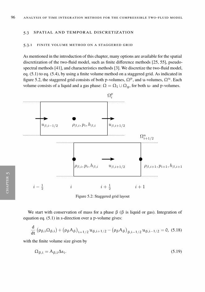
96 analysis of time integration methods for the compressible two-fluid model
chap
ter
5
5.3 spatial and temporal discretization
5.3.1 finite volume method on a staggered grid
As mentioned in the introduction of this chapter, many options are available for the spatialdiscretization of the two-fluid model, such as finite difference methods [25, 55], pseudo-spectral methods [41], and characteristics methods [3]. We discretize the two-fluid model,eq. (5.1) to eq. (5.4), by using a finite volume method on a staggered grid. As indicated infigure 5.2, the staggered grid consists of both p-volumes,Ωp, and u-volumes,Ωu. Eachvolume consists of a liquid and a gas phase:Ω = Ωl ∪Ωg, for both u- and p-volumes.
Figure 5.2: Staggered grid layout
We start with conservation of mass for a phase β (β is liquid or gas). Integration ofequation eq. (5.1) in s-direction over a p-volume gives:
ddt(ρβ,iΩβ,i
)+(ρβAβ
)i+1/2
uβ,i+1/2−(ρβAβ
)β,i−1/2 uβ,i−1/2 = 0, (5.18)
with the finite volume size given by
Ωβ,i = Aβ,i∆si. (5.19)
[ January 15, 2020 at 7:46 – classicthesis version 2.2 ]

chapter5
5.3 spatial and temporal discretization 97
The term (ρβAβ)i+1/2 requires interpolation from neighbouring values, which is de-scribed below. For conservation of momentum we proceed in a similar way. Integrationof eq. (5.3) in s-direction over a u-volume gives:
ddt(ρβ,i+1/2uβ,i+1/2Ωβ,i+1/2
)+(ρβAβ
)i+1
(uβ,i+1)2−(ρβAβ
)i(uβ,i)
2 =
−Aβ,i+1/2 (pi+1 − pi) + LGβ,i+1/2 − ρβ,i+1/2Ωβ,i+1/2gs−∑γ∈L,G,Wγ 6=β
τβγ,i+1/2Pβγ,i+1/2∆si+1/2 +Aβ,i+1/2Fbody∆si+1/2, (5.20)
where
Ωβ,i+1/2 = Aβ,i+1/2∆si+1/2, (5.21)
and the level gradient terms for the gas and liquid are given by (+ for gas, - for liquid)
LGβ,i+1/2 = g cos(ϕ)((hAβ ±
1
12P3gl
)i
−
(hAβ ±
1
12P3gl
)i−1
), (5.22)
Several terms in eq. (5.18) and eq. (5.20) require approximation. All terms that are notpart of the convective terms are interpolated using a central scheme, e.g. Aβ,i+1/2 =12(Aβ,i +Aβ,i+1). The convective terms, on the other hand, require more care in orderto prevent numerical oscillations. Since the system under consideration is (conditionally)hyperbolic, the wave directions have to be taken into account in the differencing scheme,e.g. by using a Roe method [3, 65]. In this work the focus is on the time integration methodand we employ standard spatial discretization methods for the convective quantities: firstorder upwind or second-order central. The central scheme is accurate and stable in ourcomputations since the solutions to the test cases are sufficiently smooth, i.e. we are notsimulating discontinuities or flow transitions.The spatial discretization presented in this section leads to a semi-discrete system, only
depending on time, which can be written as
dUdt
= F(U), (5.23)
where U = U(t) ∈ RqN is the vector of conserved variables. For periodic boundaryconditions, which we will consider, it reads
U =
[(ρgAg∆s)1...N, (ρlAl∆s)1...N,
(ρgAgug∆s)1/2...N−1/2, (ρlAlul∆s)1/2...N−1/2
]T. (5.24)
We useU instead ofW in a discrete setting to ensure discrete conservation properties.
[ January 15, 2020 at 7:46 – classicthesis version 2.2 ]

98 analysis of time integration methods for the compressible two-fluid model
chap
ter
5
5.3.2 temporal discretization
Equation eq. (5.23) forms a system of ordinary differential equations which can be in-tegrated in time with many different time integration methods [11, 31]. A common dis-tinction is between multi-stage methods (Runge-Kutta) and multi-step methods (Adams,Backward Differentiation Formula (BDF)). Within both classes there is a distinction be-tween explicit and implicit methods. Due to the strong time step restriction for explicitmethods (caused by the acoustic speeds λ1 and λ4), we consider implicit methods. Forthe two-fluid model, the Backward Euler method is widely applied because of its uncon-ditional numerical stability characteristics, although it has the disadvantage of being onlyfirst-order accurate, which introduces a significant amount of numerical diffusion. To con-struct a second-order method that keeps good stability properties, we consider the Crank-Nicolson and BDF2 methods, which are both second-order accurate and unconditionallystable. Backward Euler, Crank-Nicolson and BDF2 can all be gathered under the followingexpression:
a0Un+1 + a1U
n + a2Un−1
∆t= θF(Un+1, tn+1) + (1− θ)F(Un, tn). (5.25)
with the parameter values given in table 5.2.
Table 5.2: Parameter values for time integration methods.
scheme a0 a1 a2 θ
Backward Euler 1 −1 0 1
BDF2 32 −2 1
2 1
Crank-Nicolson 1 −1 0 12
Equation eq. (5.25) is a system of nonlinear equations and application of Newton’smethod leads to the following linear system that is solved at each time step:[
a0∆tI− θ
(∂F
∂U
)m]∆U =
−[a0Um + a1U
n + a2Un−1
∆t− θF(Um, tn+1) − (1− θ)F(Un, tn)
],
(5.26)
wherem is the iteration counter. If the direct evaluation of F in terms ofU is not possible- for example in the case of a nonlinear equation of state, when the pressure cannot easilybe obtained from the density - we solve equation eq. (5.26) in terms ofW, which requiresthe evaluation of an additional Jacobian. Solving system eq. (5.26) has roughly the samecomputational cost for Backward Euler, Crank-Nicolson and BDF2. This is because the
[ January 15, 2020 at 7:46 – classicthesis version 2.2 ]

chapter5
5.4 von neumann analysis on the fully discrete equations 99
evaluation of the Jacobian is the most expensive part, which is the same for all methodssince they are all implicit in time. From an implementation point of view, BDF2 can beimplemented relatively easily in an existing code that uses Backward Euler, because theonly extra required variable isUn−1.
The BDF2 method suffers from a start-up problem: Un−1 is not available at the firsttime step, which is therefore computed with Backward Euler. Note that for variable timesteps the coefficients of the BDF2 method become dependent on the time step ratio. An-other issue of BDF2 is the fact that it is not unconditionally monotone (neither is Crank-Nicolson), and therefore under- or overshoots can appear near discontinuities [43, 102].Adaptive time stepping or locally using Backward Euler are possible solutions to this issue.In the test cases reported here this was not required.
5.4 von neumann analysis on the fully discrete equations
5.4.1 introduction
In the previous sections the eigenvalues of the continuous and semi-discrete equationswere discussed. In the fully discrete case a stability analysis can be performed that isvery similar to the one applied to the continuous case (section 5.2.3). This is known asvon Neumann stability analysis [66], which can be seen as the discrete counterpart of theKelvin-Helmholtz stability analysis [2]. It is applicable in case of linear, constant coeffi-cient partial differential equations with periodic boundary conditions. We employ there-fore the linearized equations in order to be able to apply the von Neumann analysis. Asan example, we first consider the equations that result from applying the Backward Eulermethod:
Un+1 − Un
∆t= JUn+1, (5.27)
where U contains the conservative variables defined on the staggered grid as shown infigure 5.2.
In the von Neumann analysis, which is essentially a discrete Fourier analysis [66], thesolution is assumed to consist of a finite sum of discrete waves, each with a different wavenumber:
Uni =∑m
(Vni )m, (5.28)
(Vni )m = eIkmsi vnm = eIkmsi Gnm vm, (5.29)
where m indicates the mode number, km the wave number of mode m, G ∈ Cq×q theamplification matrix of mode m, and vm ∈ Cq the Fourier coefficients of mode m ofthe initial condition. q = 4 is the dimension of the problem. The fact that we employ
[ January 15, 2020 at 7:46 – classicthesis version 2.2 ]

100 analysis of time integration methods for the compressible two-fluid model
chap
ter
5
an amplification matrix is similar to the approach followed by Fullmer et al. [25], butslightly different from the scalar amplification factor considered by Liao et al. [55]. Wewill comment later on the relation between the two.
Since equation eq. (5.27) is linear it suffices to consider a single mode (Vni )m (consist-ing of solution components at grid points i and i+ 1/2 due to the staggering) to analysethe stability properties of the discretization method:
V1,i
V2,i
V3,i+1/2
V4,i+1/2
n+1
m
−
V1,i
V2,i
V3,i+1/2
V4,i+1/2
n
m
= ∆t
N∑j=1
Jij
V1,j
V2,j
V3,j+1/2
V4,j+1/2
n+1
m
. (5.30)
Since J contains the spatial discretization it is very sparse. Substituting the Fourier ex-pansion eq. (5.29) into equation eq. (5.30), omitting the subscript m, and dividing eachequation by the complex exponential in space, yields the compact expression
v1,i
v2,i
v3,i+1/2
v4,i+1/2
n+1
−
v1,i
v2,i
v3,i+1/2
v4,i+1/2
n
= ∆tM(eIkmsi)
v1,i
v2,i
v3,i+1/2
v4,i+1/2
n+1
. (5.31)
The full matrix is similar to the one presented by Liao et al. [55], but much more elaboratedue to the fact that we employ a 4× 4 system including compressibility effects. In section5.4.3 a method will be proposed which circumvents the explicit formulation of this matrix.We write equation eq. (5.31) in the following generic form, using a notation similar toFullmer et al. [25]:
Nvn+1 = Ovn, or vn+1 = N−1Ovn, (5.32)
where for Backward Euler:N = I−∆tM, andO = I. The amplification matrix is givenby
G = N−1O. (5.33)
Stability depends on the spectral radius ofG, i.e. the maximum absolute value of the (com-plex) eigenvalues λG ofG. These eigenvalues λG follow from the eigenvalue problem
det(NλG −O) = 0, (5.34)
and a scalar amplification factor can be defined as G = maxi |λG,i|. The amplificationmatrix G is the one used by Fullmer et al. [25], whereas the amplification factor λG isused by Liao et al. [55]. G contains the growth and frequency components of all waves,
[ January 15, 2020 at 7:46 – classicthesis version 2.2 ]

chapter5
5.4 von neumann analysis on the fully discrete equations 101
which allows the reconstruction of the full solution, which is not possible with λG. Insection 5.4.3 we will obtain the amplification factors from simulation data only, and thisrequires the use of the fullG.
Once the amplification matrix G and the Fourier coefficients v of the initial conditionare known, the solution at a time instance tn in terms of Fourier coefficients is obtainedfrom
vnm = Gnm vm, or vn+1m = Gm vnm. (5.35)
G contains information about the growth of the solution (diffusive errors), and about theshift (dispersive errors) of the solution in time.
5.4.2 extension to bdf2 and crank-nicolson
For the BDF2 scheme, equation eq. (5.31) becomes
Nvn+1 +Ovn +Pvn−1 = 0, (5.36)
whereN = a0I−∆tM,O = a1I, P = a2I. This equation can be written as(a0I−∆tM 0
0 I
)(vn+1
vn
)=(
−a1I −a2I
I 0
)(vn
vn−1
), or: Nwn+1 = Own, (5.37)
from which the definition ofG follows:
G = N−1O =
(−a1(a0I+M)−1 −a2(a0I+M)−1
I 0
). (5.38)
This is a particular case of the more generic linear multistep methods analysed in [43].The eigenvalues ofG follow from the determinant equation
det(NλG − O) = det((a0I−∆tM)λ2G + a1λGI+ a2I) = 0. (5.39)
When including the Crank-Nicolson method this can be generalized to
det(a0 + a1G
−1 + a2G−2
∆tI−
(θM+ (1− θ)MG−1
))= 0, (5.40)
where we write G instead of λG.
[ January 15, 2020 at 7:46 – classicthesis version 2.2 ]
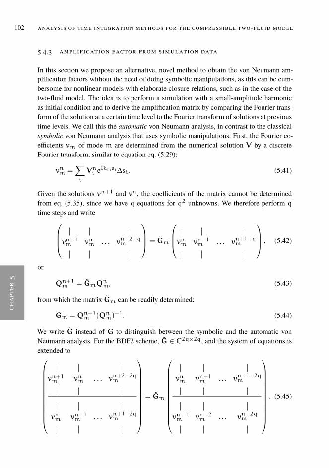
102 analysis of time integration methods for the compressible two-fluid model
chap
ter
5
5.4.3 amplification factor from simulation data
In this section we propose an alternative, novel method to obtain the von Neumann am-plification factors without the need of doing symbolic manipulations, as this can be cum-bersome for nonlinear models with elaborate closure relations, such as in the case of thetwo-fluid model. The idea is to perform a simulation with a small-amplitude harmonicas initial condition and to derive the amplification matrix by comparing the Fourier trans-form of the solution at a certain time level to the Fourier transform of solutions at previoustime levels. We call this the automatic von Neumann analysis, in contrast to the classicalsymbolic von Neumann analysis that uses symbolic manipulations. First, the Fourier co-efficients vm of mode m are determined from the numerical solution V by a discreteFourier transform, similar to equation eq. (5.29):
vnm =∑i
Vni eIkmsi∆si. (5.41)
Given the solutions vn+1 and vn, the coefficients of the matrix cannot be determinedfrom eq. (5.35), since we have q equations for q2 unknowns. We therefore perform q
time steps and writevn+1m vnm . . . vn+2−qm
= Gm
vnm vn−1m . . . vn+1−qm
, (5.42)
or
Qn+1m = GmQnm, (5.43)
from which the matrix Gm can be readily determined:
Gm = Qn+1m (Qnm)−1. (5.44)
We write G instead of G to distinguish between the symbolic and the automatic vonNeumann analysis. For the BDF2 scheme, G ∈ C2q×2q, and the system of equations isextended to
vn+1m vnm . . . vn+2−2qm
vnm vn−1m . . . vn+1−2qm
= Gm
vnm vn−1m . . . vn+1−2qm
vn−1m vn−2m . . . vn−2qm
. (5.45)
[ January 15, 2020 at 7:46 – classicthesis version 2.2 ]

chapter5
5.5 results for various test cases 103
In order to construct Qn+1m and Qnm, it suffices to take 2q time steps and to store theFourier coefficients at each time step (of course, one can also store the entire solution andcalculate the Fourier coefficients afterwards). Once G is determined, the absolute valueof its eigenvalues can be investigated. This has to be done for all wavenumbers, either byrerunning the simulation with an initial condition for each different wave, or performingone simulation with a single initial condition composed of all wavenumbers. This is asimple and fast procedure given that only 2q = 8 time steps are necessary to reconstructG. In practice, we have noted that due to the high condition number of Qn inaccurateresults are sometimes obtained. This can be resolved by increasing the number of timeinstances in the analysis to for example 4q, which works well in our simulations. ThematricesQn andQn+1 then become non-square and the solution of eq. (5.45) should beinterpreted in a least-squares sense.
To summarize, in this section we have explained two techniques, symbolic and auto-matic von Neumann analysis. This will be demonstrated for the Kelvin-Helmholtz insta-bility case in section 5.5.1. The first is the classic analysis: substitution of a Fourier seriesin the discretization matrix and investigating the resulting amplification matrix and itseigenvalues. We have done this by using the symbolic toolbox of Matlab and by direct sub-stitution of the complex exponentials into our code to arrive at symbolic expressions forthe amplification matrix. The second technique is based on substituting sinusoidal waveperturbations in the initial conditions, and running the code for several time steps. Thiscan be used to check the outcome of the first technique, but also to obtain amplificationmatrices for black-box solvers (for instance commercial codes).
5.5 results for various test cases
In this section we report the results of three test cases. The first two are related to theKelvin-Helmholtz instability: the first one considers steady state flow with a small but un-stable perturbation in a single wave to validate the linear stability (von Neumann) and ac-curacy of the time integration methods. The second case considers the same instability butwith a much larger perturbation to study the nonlinear wave growth and the identificationof ill-posedness. Lastly, in the third test case the propagation of a hold-up wave is investi-gated, and all the previously investigated concepts of stability, accuracy, ill-posedness areconsidered. The four cases will be referred to as A, B, C, and D, respectively.
[ January 15, 2020 at 7:46 – classicthesis version 2.2 ]

104 analysis of time integration methods for the compressible two-fluid model
chap
ter
5
5.5.1 kelvin-helmholtz: linear wave growth
5.5.1.1 Modified wave number analysis
We consider the Kelvin-Helmholtz instability for the test problem described in section5.2.4 and with the conditions given in table 5.1. The exact solution to the linearized systemof equations eq. (5.13) is given by
W(s, t) =W0 +∑j
Re[εje
I(ωjt−ks)]
. (5.46)
The initial condition is obtained by a small perturbation in the liquid hold-up: αl = 10−6.The perturbation vector ε3 is taken to be the eigenvector associated to the angular fre-quencyω3 [55]:
ε3 = 10−4
1 · 10−2
7.005 · 10−3 − 1.1025 · 10−3I2.497 · 10−1 + 1.186 · 10−3I
−3.619− 6.550 · 10−1I
. (5.47)
Firstly, we perform a consistency check: simultaneous grid and time step refinement fora fixed wave number k = 2π with
Cl ≈ 1→ ∆t ≈ ∆s = 1
N, (5.48)
where C is the dimensionless time step, similar to the CFL number (which strictly is astability condition). k = 2π is the smallest wave number that can presented on our pe-riodic simulation domain. The exact growth rate, Im(ω3) = −0.35, is compared to thenumerically computed growth rates as obtained from the symbolic and the automatic vonNeumann analysis:
ωvN =ln (min (Im (λ(Gm))))
∆t, ωvN =
ln(min
(Im(λ(Gm)
)))∆t
. (5.49)
Even though only a single wave is triggered due to the initial perturbation in ε3, the dis-crete amplification matrix G still has four eigenvalues. This is because the Fourier trans-form of the initial condition does not consist of a single wave, but of four waves. We areinterested in the one that is largest in magnitude, since it indicates whether the numericalsolution is stable or not. However, in contrast to the classical von Neumann analysis, inthis study unstable solutions are not necessarily unwanted, since the differential equationitself has an unstable behaviour [25], which might be associated to slug flow.Figure 5.3 shows the comparison of ω3 to ωvN and ωvN, for different grids and dis-
cretization schemes. Figure 5.3a shows that all time discretization methods converge to
[ January 15, 2020 at 7:46 – classicthesis version 2.2 ]

chapter5
5.5 results for various test cases 105
the exact growth rate upon grid refinement. However, for coarse grids, the Backward Eu-ler method predicts a positiveω (damped solutions), whereas BDF2 and Crank-Nicolsoncorrectly predict growing solutions (albeit with a reduced growth rate). In figure 5.3b thisis made more quantitative by computing the error of the discrete models compared to theexact value:
η = |ω3 −ωvN|. (5.50)
It is clear that the use of Backward Euler or the use of the first order upwind scheme limitsthe accuracy to first order. Figure 5.3b also indicates that for very fine meshes there is aslight discrepancy between the symbolic and automatic von Neumann analysis. This isrelated to the matrix inversion required for the reconstruction eq. (5.44) in the automaticvon Neumann analysis, which can suffer from numerical inaccuracies. For the main pur-pose of the von Neumann analysis, namely investigating the behaviour of the numericalgrowth rate or dispersion error as function of phase angle (φ = k∆s), this is not an issue.
Secondly, we investigate howwaves grow in time, depending on the wave number k andthe spatial and temporal discretization. The number of grid points is fixed (∆s = 1/160
m). The shortest wavelength that can be represented on the grid is 2∆s (Nyquist limit),corresponding to the wavenumber k = π/∆s, and phase angle φ = π. The wave numberanalysis provides insight into how well waves of different frequency are resolved by thetime integrationmethod. It is similar to the analysis for spatial discretizationmethods doneby Liao et al. [55]. Figure 5.4a shows the growth rate G = max |λ(G)| which compareswell with the results of [55]. In addition, figure 5.4b shows the growth rateωvN instead ofthe amplification factor, which includes the exact solution (denoted by the black dashedline). It is perhaps not surprising to see that Crank-Nicolson (‘central in time’) with acentral scheme in space leads to an accurate prediction of G. In fact, when performingthe analysis without friction terms (in the well-posed stable regime), the Crank-Nicolson /central combination leads toG = 1 independent of the wavenumber. This is a well-knownresult for advection equations and also holds for the two-fluid model without source terms.However, the presence of source terms leads to unstable solutions; their growth rate canbe captured by the numerical scheme though, with the accuracy of the time integrationmethod. Furthermore, G = 1 does not mean that the numerical is exact, but that there areonly dispersive errors and no diffusive errors.For each wavenumber k the corresponding growth rate ω3 is negative. This agrees
with the stability-hyperbolicity theorem [73] which says that the neutral stability limit isindependent of the wavenumber. The case of k = 2π from figure 5.3 is highlighted asthe black vertical line in figure 5.4. For φ < 10−2 all numerical methods perform well -this corresponds to long, low frequency waves which are well resolved. For larger φ thenumerical damping of all methods becomes apparent. The kinks in the amplification factorand the growth rate are due to the fact that a different eigenvalue (see equation eq. (5.49))becomes dominant.
[ January 15, 2020 at 7:46 – classicthesis version 2.2 ]
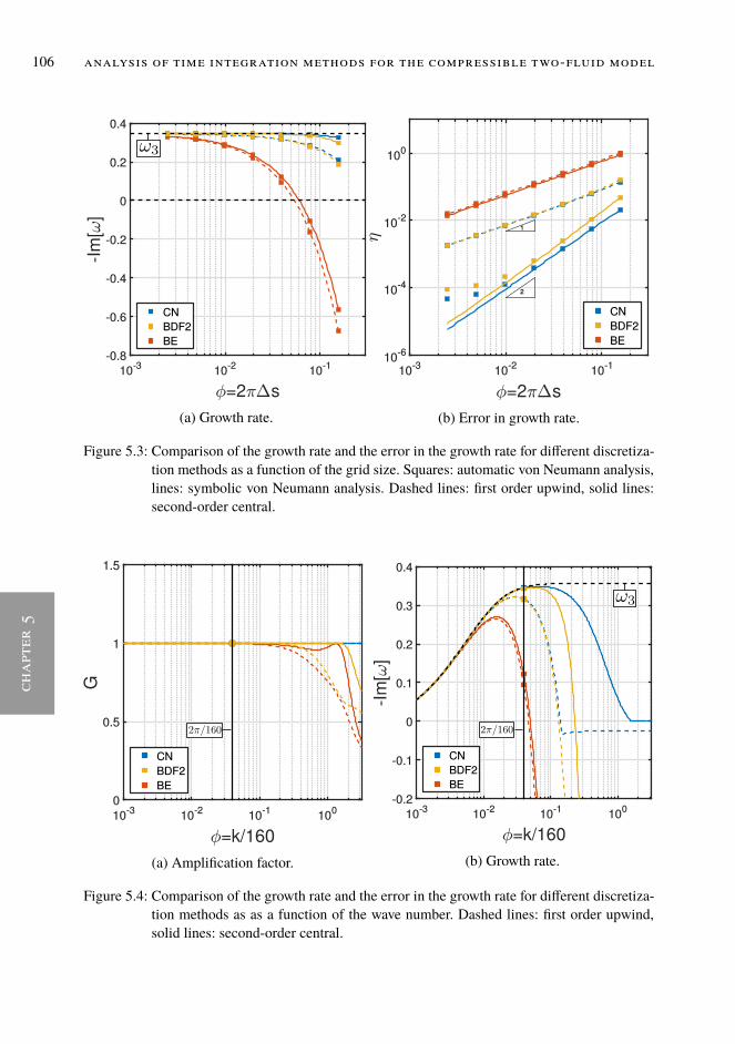
106 analysis of time integration methods for the compressible two-fluid model
chap
ter
5
(a) Growth rate. (b) Error in growth rate.
Figure 5.3: Comparison of the growth rate and the error in the growth rate for different discretiza-tion methods as a function of the grid size. Squares: automatic von Neumann analysis,lines: symbolic von Neumann analysis. Dashed lines: first order upwind, solid lines:second-order central.
(a) Amplification factor. (b) Growth rate.
Figure 5.4: Comparison of the growth rate and the error in the growth rate for different discretiza-tion methods as as a function of the wave number. Dashed lines: first order upwind,solid lines: second-order central.
[ January 15, 2020 at 7:46 – classicthesis version 2.2 ]

chapter5
5.5 results for various test cases 107
5.5.1.2 Linearized discrete flow pattern map prediction
In this section we propose a novel way for displaying the performance of numerical meth-ods, which we call ‘Discrete Flow Pattern Maps’ (DFPM), that uses the growth rate deter-mination method developed for the automatic von Neumann analysis (equation eq. (5.44)).Whereas traditional flow pattern maps, such as the one in figure 5.1, display stable andunstable regimes based on the properties of the differential equations, the DFPM displaysthe effective stability regions that result when the discrete equations are solved, with acertain numerical method and a certain grid and time resolution. Such a map is of crucialimportance as an indication whether a discretization method is able to correctly capturethe well-posed unstable regime (and the potential transition to slug flow) or whether nu-merical diffusion overwhelms the physical growth of instabilities.The DFPM can be constructed in the sameway in which we constructed the flow pattern
map in figure 5.1. We employ a sequence of superficial liquid and gas velocities, solve thediscrete equations with a small perturbation as initial condition and determine the growthrate ωvN from eq. (5.44) and eq. (5.49). The stability boundary is given by Im(ωvN) = 0.Figure 5.5a shows the VKH stability boundary for Backward Euler and BDF2 for twodifferent grids (and associated time steps). It can be seen that BDF2 captures the exactstability boundary very accurately on all grids. On the other hand, the effective stabilityregion given by Backward Euler is much larger (note the log scale) than the actual stabilityregion of the differential equations, due to the large amount of artificial diffusion addedby Backward Euler. For example, for N = 40, and at a superficial gas velocity of usg =
10 m/s, the two-fluid model predicts growing waves at a superficial liquid velocity ofusl = 0.15 m/s, but with Backward Euler the wave growth is only apparent when thesuperficial liquid is increased to usl = 0.6 m/s (already at the ill-posed boundary).
Any simulation starting above the ill-posedness boundary will directly be marked as ill-posed, because our ill-posedness indicator is based on the evaluation of the eigenvaluesof the differential equations, see equation eq. (5.12). However, it is possible that, due tononlinear effects, simulations that start in the well-posed unstable regime grow into theill-posed regime. This is investigated in the next section.
5.5.2 kelvin-helmholtz: nonlinear wave growth
In this section the simulation from section 5.5.1 is repeated, but with a larger perturbation:αl = 10−2, and ε3 = 104ε3. This causes the simulation to quickly enter the nonlinearregime, where waves steepen, possibly leading to slug formation but potentially also to ill-posedness. Based on the results of the previous section, we select BDF2 with N = 80 toassess the growth of initial perturbations into the nonlinear regime and whether this leadsto ill-posed results. Note that this is different from a previous study [33], in which wehave assessed the ‘time to ill-posedness’ as a metric to compare different time integration
[ January 15, 2020 at 7:46 – classicthesis version 2.2 ]

108 analysis of time integration methods for the compressible two-fluid model
chap
ter
5
methods. In the present study the focus is on whether well-posed unstable solutions canbe obtained for long time integration periods.
Similar to the linear case, we perform simulations with the two-fluid model with a cen-tral discretization for a range of superficial gas and liquid velocities but now until t = 100s and only with a central discretization of the convective terms. Ill-posedness is investi-gated by checking if the eigenvalues of the differential equation are real or complex at theconditions predicted by the numerical simulation. If a complex eigenvalue occurs at anypoint in space or time the corresponding point in the flow pattern map is marked ill-posed.Figure 5.5b shows that the resulting numerical ill-posedness boundary has shifted signifi-cantly into the well-posed unstable regime as compared to the ill-posedness boundary ofthe differential equations (indicated by IKH in figure 5.5b). It appears that a large partof the well-posed unstable regime of the flow pattern map gives ill-posed solutions whenactual numerical simulations are performed. An example of a simulation which turnsill-posed is case A in figure 5.5b, which corresponds to the conditions studied in section5.5.1 for linear perturbations. The nonlinear behaviour of the hold-up fraction αl in spaceand time is shown in figure 5.6 for this case. The solution becomes ill-posed already afterapproximately 5 seconds. The liquid hold-up fraction as a function of time at s = 1 m isshown in figure 5.7a.In addition to case A, three other cases (B, C, and D) are indicated in figure 5.5b which
exhibit qualitatively different solution behaviour. Case B in figure 5.7b starts in the well-posed unstable regime, like case A, but after initial growth (as predicted by linear theory)stabilizes and forms a wave with a constant amplitude and frequency. Its shape and posi-tion in the flow pattern map indicate that this could be a so-called continuous ‘roll wave’:a particular solution to the two-fluid model which is constant in a reference frame movingwith the flow [6, 41, 48]. To check that this is not a numerical artefact, we have confirmedthe roll wave presence with a simulation on a much finer grid (N = 640). Case C andD are both in the well-posed stable regime, where initial perturbations are damped ac-cording to the linear theory. This happens indeed for case D. However, for case C, thedamping is very small (Im(ω3) = 0.01) and nonlinear effects lead to wave growth andthe appearance of new harmonics. The oscillation frequency is now lower because the realpart ofω3 has decreased. Within the time period of 100 seconds displayed in the plot it isunclear if the wave damps out. Continued simulation until 1000 seconds reveals that thewave eventually damps out, like in case D.
We note that the current simulation results are obtained based on a number of simplifi-cations compared to pipeline simulations on actual geometries. First, we employed initialperturbations according to the eigenvector ε3. This means that the perturbations immedi-ately grow according to linear theory until nonlinear effects take over. Second, we used asingle wave with wavenumber k = 2π. Other wavenumbers will have different frequen-cies and growth rates and can lead to qualitatively different behaviour (although the VKHand IKH boundaries are independent of wavenumber). Furthermore, the periodic bound-ary conditions and size of the domain limit the frequencies that can be represented on the
[ January 15, 2020 at 7:46 – classicthesis version 2.2 ]

chapter5
5.5 results for various test cases 109
domain. Lastly, we note the black region in figure 5.5b, which indicates the region wherethe liquid reaches the top of the pipeline. This is not necessarily ill-posed, but outside thescope of our investigation.
(a) Effect of time integration methods and reso-lution.
(b) Effect of nonlinear growth.
Figure 5.5: Discrete flow pattern maps (DFPM).
6
4
t [s]2
01
0.8
0.6
s [m]
0.4
0.2
0.5
0.6
0.4
0
αl[-]
Figure 5.6: Solution in space and time for case A, simulated with BDF2: well-posed unstable so-lution becoming ill-posed (indicated in red). The blue curve is shown in figure 5.7a.
[ January 15, 2020 at 7:46 – classicthesis version 2.2 ]
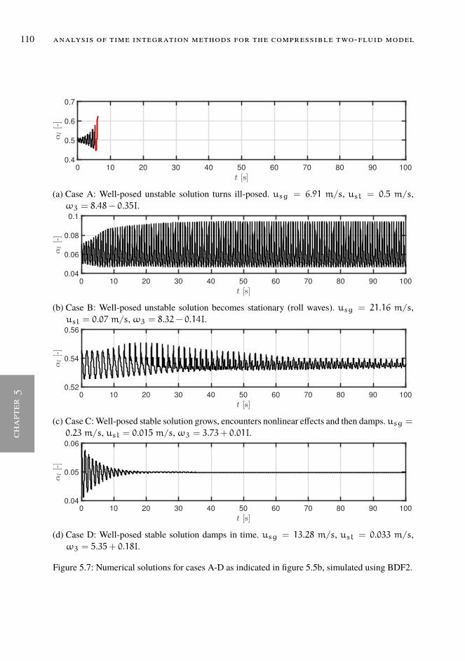
110 analysis of time integration methods for the compressible two-fluid model
chap
ter
5
t [s]0 10 20 30 40 50 60 70 80 90 100
αl[-]
0.4
0.5
0.6
0.7
(a) Case A: Well-posed unstable solution turns ill-posed. usg = 6.91 m/s, usl = 0.5 m/s,ω3 = 8.48− 0.35I.
t [s]0 10 20 30 40 50 60 70 80 90 100
αl[-]
0.04
0.06
0.08
0.1
(b) Case B: Well-posed unstable solution becomes stationary (roll waves). usg = 21.16 m/s,usl = 0.07 m/s,ω3 = 8.32− 0.14I.
t [s]0 10 20 30 40 50 60 70 80 90 100
αl[-]
0.52
0.54
0.56
(c) Case C:Well-posed stable solution grows, encounters nonlinear effects and then damps. usg =
0.23 m/s, usl = 0.015 m/s,ω3 = 3.73+ 0.01I.
t [s]0 10 20 30 40 50 60 70 80 90 100
αl[-]
0.04
0.05
0.06
(d) Case D: Well-posed stable solution damps in time. usg = 13.28 m/s, usl = 0.033 m/s,ω3 = 5.35+ 0.18I.
Figure 5.7: Numerical solutions for cases A-D as indicated in figure 5.5b, simulated using BDF2.
[ January 15, 2020 at 7:46 – classicthesis version 2.2 ]
chapter5
5.6 conclusions 111
5.6 conclusions
In this chapter we have analysed several time integration methods for the compressibletwo-fluid model with the goal to simulate stratified wavy flow and slug flow in pipelinesin a so-called ‘slug capturing’ approach. The study was focussed on obtaining insight intothe numerical pitfalls and requirements. Thereto a theoretical analysis on the differentialequations and the discretized equations was given, in particular with respect to their sta-bility properties. The analysis has been demonstrated for a number of test cases.We conclude that the BDF2 method is a robust time integrator for the two-fluid model
and it outperforms the commonly used Backward Euler method and the second-orderCrank-Nicolson method. This is due to a combination of its second-order accuracy, A-stability and L-stability. These properties make that BDF2 can be used for the time inte-gration of unsteady problems with a CFL number of 1 based on the liquid velocity, whilenot suffering from numerical oscillations that arise from acoustic wave propagation.To facilitate the comparison and understanding of the time integration methods, sev-
eral techniques have been proposed which have not been applied to the two-fluid modelbefore. First, a new automatic von Neumann analysis technique has been developed as toolfor direct evaluation of the stability of the discrete models by running a computer codewithout requiring symbolic manipulations. This makes it very flexible since it can be di-rectly applied when more physics (e.g. surface tension or axial diffusion) or other spatialdiscretization methods are included. Second, we have proposed the use of Discrete FlowPattern Maps (DFPM) to indicate to what extent discretization methods (for a certainchoice of the number of grid points and the size of the time step) are able to reproduce theflow pattern maps that are based on the stability of the differential equations. The DiscreteFlow Pattern Map reveals that the effective well-posed unstable region is well captured byBDF2 but completely missed by Backward Euler, at least for the considered grid and timestep resolutions. Simulations in the nonlinear regime furthermore have indicated that ill-posedness can occur when starting from the unstable regime. The implication is that theactual well-posed unstable regime for nonlinear simulations can be much smaller than thetheoretical one, which can limit the application of the two-fluid model for simulating thestratified-slug flow transition.We note that the DFPM as presented here is based on simulations in an idealized set-
ting, with a simple geometry, initial conditions, and boundary conditions. In future workwe plan to employ the BDF2 method to further study the formation of slug flow and ill-posedness issues under actual pipeline conditions.
[ January 15, 2020 at 7:46 – classicthesis version 2.2 ]

[ January 15, 2020 at 7:46 – classicthesis version 2.2 ]

chapter6
6MODELL ING OF BY- PASS P IGG ING IN TWO-PHASESTRAT I F I ED P I PE FLOW
This chapter is adopted fromM.H.W. Hendrix, H.P. IJsseldijk, W.-P. Breugem, and R.A.W.M. Henkes, "Sim-ulation of slug propagation for by-pass pigging in two-phase stratified pipe flow". In: 19th InternationalConference on Multiphase Technology (2019), pp. 317-330.
113
[ January 15, 2020 at 7:46 – classicthesis version 2.2 ]

114 modelling of by-pass pigging in two-phase stratified pipe flow
chap
ter
6
6.1 introduction
Several efforts have been made in the past to model the trajectory of a pig, which is pro-pelled by the fluids in a pipeline. These efforts often rely on a 1D cross-sectional descrip-tion of the fluid, while the pig is modelled as a point mass. The reason for this simplifiedapproach is the high aspect ratio of the problem, which leads to an approach which onlyconsiders variations in the direction of the curvilinear coordinate s that runs along thepipeline. Such a 1D approach for the motion of two fluids in a pipeline has been describedin chapter 5. The incorporation of a pig in a 1D approach for single phase flow has beenbriefly discussed in chapter 4. In this chapter we provide more details of the numericalimplementation, and focus on the development of a 1D numerical model for pig motionin two-phase flow.Kohda et al. [50] were among the first to present a numerical method for the motion
of a pig in two-phase pipe flow. A separate coordinate system is used for the pig and thefluid. Their simulation results appeared to be in good agreement with experimental data.However, no details were provided on how the two used coordinate systems are coupled.The incorporation of a by-pass in the pig body using a 1D transient single-phase piggingmodel has been proposed by Nguyen et al. [67], who employed a method of characteristics(MOC) to solve the hyperbolic partial differential equations. Esmaeilzadeh et al. [22] useda MOC approach to model pig motion in a single phase pipeline, while comparing themodeling results to field data. Nieckele et al. [69] and Hosseinalipour et al. [42] used afinite difference technique to model the motion of a by-pass pig in a single-phase pipeline.Both studies address the necessity of regridding the numerical grid by using an adaptivemesh as the pig moves through the pipe, but it is not clear whether the approaches are massconservative. Most of the studies for 1D pig modelling in a pipeline focus on single-phaseflow, only a few consider the presence of a second phase [47, 50, 61, 97]. Among thesestudies that considered two-phase flow, only pigs without by-pass are considered.This chapter describes the development of an accurate 1D numerical method to solve
the motion of a pig with and without by-pass in a two-phase pipeline. The pig is imple-mented as a moving border of the numerical grid on which the two-fluid model is solvedusing a finite-volumemethod. The two-fluid model has been described in chapter 5 for usecases with periodic boundary conditions. This is clearly not applicable for monitoring thetrajectory of a pig through a pipeline: we will need appropriate boundary conditions at theinlet and outlet of the pipe. We propose the use of characteristic boundary conditions [71,88]. A similar approach is used to handle the boundary conditions on both sides of the pig.As the pig traverses through the pipe, it is necessary to regrid the finite volumes aroundthe pig, to ensure that the finite-volume sizes do neither get too large nor too small.The structure of this chapter is as follows. The numericalmethod covering the discretiza-
tion and boundary treatment is discussed in section 6.2. The pig motion is described byNewton’s second law. To account for different types of friction (static vs. dynamic), asmooth function is designed which addresses the different types of friction. Some mod-
[ January 15, 2020 at 7:46 – classicthesis version 2.2 ]

chapter6
6.2 numerical method 115
elling results have already been shown in chapter 4, but more details on the numericalimplementation are given in 6.3. Test cases considering two-phase flow will be given insection 6.4. Section 6.5 gives conclusions and discusses possibilities for further research.
6.2 numerical method
The two-fluid model which is used to model the simultaneous transport of a liquid anda gas through a pipeline has been discussed in chapter 5. In that chapter only periodicboundary conditions have been considered, and a body force Fbody was needed in themomentum equations to keep the flow going (see eq. 5.1 - 5.4). In this chapter we considerthe presence of a pig which moves through a (horizontal) pipeline, so instead of periodicboundary conditions, appropriate inlet and outlet conditions are needed. We thereforedrop the body forces, and the two-fluid equations read:
∂
∂t(ρgAg) +
∂
∂s(ρgugAg) = 0, (6.1)
∂
∂t(ρlAl) +
∂
∂s(ρlulAl) = 0, (6.2)
∂
∂t(ρgugAg) +
∂
∂s(ρgu
2gAg) = −
∂p
∂sAg +
∂HGg∂s
+(−τglPgl − τgPg
)︸ ︷︷ ︸Sg
,
(6.3)∂
∂t(ρlulAl) +
∂
∂s(ρlu
2lAl) = −
∂p
∂sAl +
∂HGl∂s
+(τglPgl − τlPl
)︸ ︷︷ ︸Sl
. (6.4)
Here Ag and Al represent the hold-up of the gas and the liquid phase, respectively. Thegas and liquid hold-up makeup the total pipe area, A = Ag +Al. The phase velocitiesfor the gas and the liquid are respectively denoted ug and ul. The density of the liquid,ρl, is taken constant, whereas the density of the gas, ρg = ρg(p), is given by the idealgas law (eq. 5.16). Here p is the pressure. HGg and HGl denote the hydraulic gradientterms, which are given by eq. 5.6 and eq. 5.7 respectively. The last two terms of Eq. 6.3and Eq. 6.4 represent an expression for the interfacial friction and wall friction. The shearstress of the gas with the pipe wall is denoted as τg and the shear stress of the liquid withthe pipe wall is denoted as τl. They are expressed by the Fanning friction factor, whichis calculated using the Churchill relation, see appendix D.2. The interfacial shear stressτgl is calculated according to [55]. Pg and Pl denote the wetted perimeters, whereas Pglrepresents the length of the gas/liquid interface within the pipe cross-sectional area, see
[ January 15, 2020 at 7:46 – classicthesis version 2.2 ]
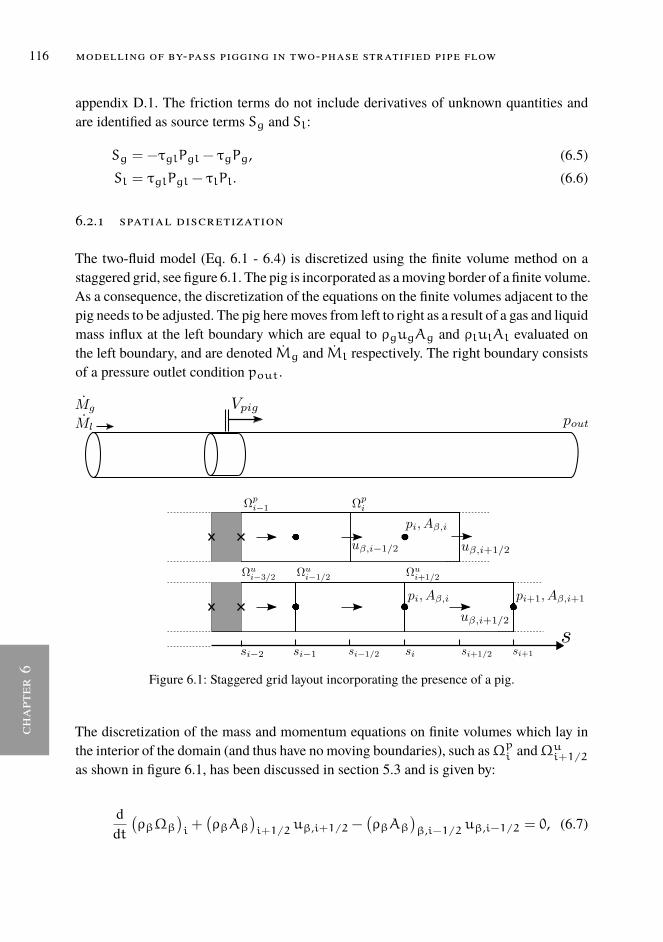
116 modelling of by-pass pigging in two-phase stratified pipe flow
chap
ter
6
appendix D.1. The friction terms do not include derivatives of unknown quantities andare identified as source terms Sg and Sl:
Sg = −τglPgl − τgPg, (6.5)Sl = τglPgl − τlPl. (6.6)
6.2.1 spatial discretization
The two-fluid model (Eq. 6.1 - 6.4) is discretized using the finite volume method on astaggered grid, see figure 6.1. The pig is incorporated as amoving border of a finite volume.As a consequence, the discretization of the equations on the finite volumes adjacent to thepig needs to be adjusted. The pig heremoves from left to right as a result of a gas and liquidmass influx at the left boundary which are equal to ρgugAg and ρlulAl evaluated onthe left boundary, and are denoted Mg and Ml respectively. The right boundary consistsof a pressure outlet condition pout.
Figure 6.1: Staggered grid layout incorporating the presence of a pig.
The discretization of the mass and momentum equations on finite volumes which lay inthe interior of the domain (and thus have no moving boundaries), such asΩpi andΩ
ui+1/2
as shown in figure 6.1, has been discussed in section 5.3 and is given by:
ddt(ρβΩβ
)i+(ρβAβ
)i+1/2
uβ,i+1/2 −(ρβAβ
)β,i−1/2 uβ,i−1/2 = 0, (6.7)
[ January 15, 2020 at 7:46 – classicthesis version 2.2 ]

chapter6
6.2 numerical method 117
ddt(ρβuβΩβ
)i+1/2
+(ρβAβu
2β
)i+1
−(ρβAβu
2β
)i=
−Aβ,i+1/2 (pi+1 − pi) +(HGβ,i+1 −HGβ,i
)+ Sβ,i+1/2, (6.8)
where
Ωβ,i = Aβ,i∆si. (6.9)
Here ∆si =(si+1/2 − si−1/2
)is the length of the finite volume. We now focus on the
discretization of finite volumes adjacent to the pig, such as Ωpi−1 and Ωui−3/2. For themoment we assume that no by-pass is present in the pig body. As a result, the discretiza-tion of the convective term results in a zero contribution from the left cell face of thefinite volume. The spatial discretization of the mass equation for phase β (where β = g
represent gas, and β = l represents liquid) onΩpi−1 then reads:
ddt(ρβΩβ
)i−1
+(ρβAβ
)i−1/2
uβ,i−1/2 = 0, (6.10)
HereΩβ,i−1 is a function of time. Similarly, the discretization of the momentum equationon the finite volumeΩui−3/2 reads:
ddt(ρβuβΩβ
)i−3/2
+(ρβAβ
)i−1
u2β,i−1 =
−Aβ,i−3/2 (pi−1 − pi−2) +(HGβ,i−1 −HGβ,i−2
)+ Sβ,i−3/2. (6.11)
Note thatpi−2 is the pressure at the downstream side of the pig. This pressure follows fromappropriate boundary conditions, which are explained in section 6.2.3. The discretizationof the finite volumes which are located on the left side of the pig are adjusted in a similarway.
6.2.2 regridding
As the pig traverses through the pipe, the finite volume in front of the pig will reduce insize and the finite volume at the back of the pig will increase in size. We solve our systemof equations in conservative form (see also section 5.3), which means that we solve for thetotal mass Umass,i = ρβ,iΩ
pi and total momentum Umom,i+1/2 =
(ρβuβΩ
u)i+1/2
.Since the size of the finite volume is part of the conservative variable Umass,i andUmom,i+1/2, the change of the size of the finite volume due to the motion of the pig isnaturally captured. The pig motion is solved by applying Newton’s second law, which wewill discuss in more detail in section 6.3. The pig position and pig velocity are appended
[ January 15, 2020 at 7:46 – classicthesis version 2.2 ]
118 modelling of by-pass pigging in two-phase stratified pipe flow
chap
ter
6
to the vector of unknowns which contains Umass,i and Umom,i+1/2 for each finite vol-ume. The resulting system of equations is solved in a monolithic fashion. Since the pigposition and pig velocity are part of the solution, there always exists a mapping of Ui tothe primitive variables uβ,i, ρβ,i and Aβ,i.As a result of the current approach, the finite volume in front of the pig will at some
point become too small, whereas the finite volume at the back of the pig will become toolarge. Therefore, the grid has to be regularly regenerated as the pig traverses through thepipe. We perform the grid regeneration as follows. When the finite-volume cell in front ofthe pig gets smaller than half the size of a cell as found in the interior, it will be mergedwith its neighbouring cell. Similarly, if the cell at the back of the pig gets larger than 1.5the size of a cell as found in the interior, it will be split up in two cells, see figure 6.2.The conservative variableUi will be reconstructed accordingly. The massU∗mass,i of thevolume in front of the pig after regeneration is determined by the sum of the masses ofthe cells before merging:
U∗mass,i+1 = Umass,i +Umass,i+1 (6.12)
The mass of the cells at the back of the pig is distributed proportionally to the length ofthe newly created cells (which are denoted ∆s∗i−1 and ∆s∗i ):
U∗mass,i−1 =∆s∗i−1Umass,i−1
∆si−1(6.13)
U∗mass,i =∆s∗iUmass,i−1
∆si−1(6.14)
The approach is mass conservative, as ∆s∗i−1 +∆s∗i = ∆si, which will be demonstratedin section 6.4.1. The merging and splitting of momentum cellsUmom,i+1/2 is performedin the same way.We integrate the system of equations in time using the BDF2 scheme, see section 5.3.2.
Before performing a new time step, the grid is regenerated if necessary. As a result of theregridding procedure as described above, we do not have the solution at the previous timestep which exists on the new grid. We therefore change the time integration scheme toBackward Euler for the first time step after regridding for all unknowns, as BDF2 cannotbe used since it needs the solution at the previous time step. After having performed thefirst time step following a regridding procedure, we switch back to the higher order BDF2scheme.
[ January 15, 2020 at 7:46 – classicthesis version 2.2 ]

chapter6
6.2 numerical method 119
Figure 6.2: Grid regeneration. (a) Grid before regeneration. (b) Grid after regeneration.
6.2.3 boundary conditions
Boundary conditions are implemented using a characteristic boundary treatment [71, 88].We first write eq. 6.1- 6.4 at a boundary point in vector form:
∂U
∂t+∂F0∂s
+D0∂W
∂s= S. (6.15)
HereU = [ρgAg, ρlAl, ρgugAg, ρlulAl]T is the vector containing the conserved vari-ables andW = [Al,p,ug,ul]T contains the primitive variables. The source terms Sgand Sl are collected in the vector S = [0, 0,Sg,Sl]T . We have collected the conservativeflux contributions into the second term of eq. 6.15. Here F0 is given by:
F0 =
ρgugAg
ρlulAl
ρgu2gAg −HGg
ρlu2lAl −HGl
. (6.16)
The non-conservative flux contributions are collected into the third term of eq. 6.15. HereD0 is given by:
D0 =
0 0 0 0
0 0 0 0
0 Ag 0 0
0 Al 0 0
. (6.17)
[ January 15, 2020 at 7:46 – classicthesis version 2.2 ]

120 modelling of by-pass pigging in two-phase stratified pipe flow
chap
ter
6
We now put eq. 6.15 in quasi-linear form by defining Jacobian matrix A0 = ∂U∂W and
J0 = ∂F0∂W :
A0∂W
∂t+ J0
∂W
∂s+D0
∂W
∂s= A0
∂W
∂t+B0
∂W
∂s= S. (6.18)
Here B0 = J0 +D0, and is given as follows:
B0 =
−ugρg Agug
∂ρg∂p Agρg 0
ulρl 0 0 Alρl
−u2gρg −∂HGg∂Al
Ag(u2g∂ρg∂p + 1) −
∂HGg∂p 2Agugρg 0
u2lρl −∂HGl∂Al
Al 0 2Alulρl
. (6.19)
We now multiply eq. 6.18 with A−10 to obtain:
∂W
∂t+Q
∂W
∂s= A−1
0 S. (6.20)
HereQ = A−10 B0 is given by:
Q =
ul 0 0 Al
−ρg(ug−ul)
Ag∂ρg∂p
ugρg∂ρg∂p
Alρg
Ag∂ρg∂p
−∂HGg∂Al
AgρgAg −
∂HGg∂p
Agρgug 0
−∂HGl∂Al
Alρl1ρl
0 ul
. (6.21)
To derive characteristic equations, from which time dependent equations for the boundarypoints can be obtained, we determine the eigendecomposition ofQ, that isQ = RΛR−1.HereΛ contains the eigenvalues [λ1, λ2, λ3, λ4]T on the diagonal andR contains the righteigenvectors ofQ:
∂W
∂t+RΛR−1∂W
∂s= A−1
0 S. (6.22)
The eigenvalues and eigenvectors can be computed analytically with the help of a com-puter algebra system (in this case Matlab version 2016b has been used). However, theexpressions which are obtained are long, so we will not reproduce them here. Now wedefine the vector L = ΛR−1 ∂W
∂s and rewrite eq. 6.22 as follows:
∂W
∂t+RL = A−1
0 S. (6.23)
[ January 15, 2020 at 7:46 – classicthesis version 2.2 ]

chapter6
6.2 numerical method 121
Here the components of L = [L1,L2,L3,L4]T are associated to the eigenvalues[λ1, λ2, λ3, λ4]T . The four eigenvalues of the compressible two-fluid model, assumingsubsonic flow, contain one negative and one positive eigenvalue close to the speed ofsound, say λ1 and λ4 respectively. The magnitude of the other two eigenvalues, λ2 andλ3 are in the order of the phase velocities and their sign depends on the local flow con-ditions [23, 80]. We thus consider the following three possibilities: λ2 and λ3 are bothpositive, λ2 and λ3 are both negative, and λ2 is negative while λ3 is positive. We use thesign of the eigenvalues to determine the number of incoming and outgoing waves at theboundary. By solving eq. 6.23 we can then formulate time dependent equations for the so-lution at the boundary points. For example, we consider the right boundary point, whichcorresponds to the outlet of the domain for the cases considered in this work. Figure 6.3shows the grid layout near the right boundary point.
Figure 6.3: Schematic of the grid layout near the right boundary point.
The eigenvalues can be calculated at the boundary point as function of the current solutionat the boundary point. A possible outcome could be that λ2 and λ3 are both positive, whichwould imply we have three positive eigenvalues and one negative eigenvalue (since λ1 andλ4 are negative and positive respectively). Since we consider the right boundary, threepositive eigenvalues correspond to three outgoing waves. This means that the componentsL2, L3 and L4 of vector L which feature ∂W∂s can be calculated by using finite differenceswhich are evaluated using the interior of the domain. L1 should not be calculated in thiscase, since it corresponds to an ingoingwave, and no information is available in the interiorof the domain. Instead information should be given by supplying an appropriate boundarycondition by providing an expression for one of the entries vector ∂W∂t . A typical boundarycondition for an outlet used in this work is an outlet condition for the pressure. A constantoutlet pressure corresponds to ∂p∂t = 0. Eq. 6.23 can now be completely solved sincewe have 4 unknowns (L1 and the remaining three unknown entries of vector ∂W∂t ) and4 equations. The result is an expression for the full vector ∂W∂t at the boundary point,
[ January 15, 2020 at 7:46 – classicthesis version 2.2 ]
122 modelling of by-pass pigging in two-phase stratified pipe flow
chap
ter
6
which can be integrated together with the interior using the BDF2 scheme. For the leftboundary of the domain and the pig boundaries we employ the same technique. For thepig boundaries this results in a boundary condition for the fluid velocity from which theliquid hold-up and pressure can be calculated. For some boundary conditions it may bemore convenient to express the boundary equations in terms of conserved variables Uinstead of primitive variablesW. For example, at the inlet of the domain one would rathersupply boundary conditions in terms of the gas and liquid mass inflow than in terms ofgas and liquid velocity. To derive boundary equations in terms ofU, eq. 6.23 is multipliedby Jacobian A0.
6.3 pig motion
The pig motion follows from Newton’s second law:
dsdt
= v, (6.24)
mdvdt
= Fp − Ffric. (6.25)
Here s and v are the pig position velocity respectively. Fp = ∆pA is the driving forcegenerated by the pressure drop∆p over the pig and Ffric is the friction force which the pigexperiences with the inner pipe wall. Whereas Fp can be evaluated by using the pressureupstream and downstream of the pig, Ffric needs to be modelled. We make a distinctionbetween the static friction Ffric,s which is valid when the pig is notmoving, and a dynamicfriction Ffric,d when the pig is moving. Ffric can thus be described by the followingequation:
Ffric =
minFp, Ffric,s if v = 0sgn(v)Ffric,d if v 6= 0.
(6.26)
Usually, Ffric,s > Ffric,d, see chapter 4, where the effect of Ffric,s on the maximum pigvelocity of a pig undergoing stick-slip motion was discussed. Eq. 6.26 is discontinuousaround v = 0, which poses a challenge when solving the pig motion numerically. Since wesolve the two-fluid equations and the pig motion in a monolithic fashion using Newton’smethod (see Eq. 5.26), we approximate eq. 6.26 with a smooth function which will aidconvergence of the solver. We will explain the construction of this smooth function inmore detail in the next section.
[ January 15, 2020 at 7:46 – classicthesis version 2.2 ]

chapter6
6.3 pig motion 123
6.3.1 a smooth function for the pig friction with the pipe wall
In order to design a smooth function which approximates eq. 6.26 we introduce the fol-lowing functions:
H1(c1, c2,w1, s1, x) = c1 +c2 − c12
(tanh
(4x− s1w1
)+ 1
), (6.27)
H2(c1, c2,w1, s1,y) = s1 +w1π
(arcsin
(2y− c1c2 − c1
− 1
)), (6.28)
H3(c1, c2,w1, s1, x) =c1 if x− s1 <
−w12
c1 +c2 − c12
(sin(πx− s1w1
)+ 1
)if |x− s1| 6
w12
c2 if x− s1 >w12
.
(6.29)
We now define an expression for the friction in three zones: a zone inwhich the pig velocityis negative, a zone in which the the pig velocity is positive, and a zone in which the pigvelocity is near zero. The friction in these three zones is defined respectively:
Ffric,1 = H1(−Ffric,d,−Ffric,s,vtrans
2,−vtrans, v), (6.30)
Ffric,2 = H1(Ffric,s, Ffric,d,vtrans
2, vtrans, v), (6.31)
Ffric,3 = H3(−Ffric,s, Ffric,s,vtrans
2, s2, v). (6.32)
Here s2 is defined as:
s2 = H2(Ffric,s,−Ffric,s,vtrans
2, 0, Fp). (6.33)
Furthermore, vtrans is a constant and is used to determine the pig velocity range overwhich the friction changes from zone to zone. In order to arrive at an expression for Ffricwhich connects the friction as defined in each of the zones, we now define two switchingfunctions:
S1 = H1(1, 0,vtrans
2,−vtrans
2, v), (6.34)
S2 = H1(0, 1,vtrans
2,vtrans
2, v). (6.35)
[ January 15, 2020 at 7:46 – classicthesis version 2.2 ]

124 modelling of by-pass pigging in two-phase stratified pipe flow
chap
ter
6
We can then construct a smooth approximation of eq. 6.26, Ffric,sm, as follows:
Ffric,sm = S1Ffric,1 + S2Ffric,2 + (1− S1)(1− S2)Ffric,3. (6.36)
Figure 6.4 shows eq. 6.36 evaluated as function of the pig velocity v and the driving forceFp. Here we took Ffric,s = 40.3 N, and Ffric,s = 48 N, which represent values as usedin section 4.4.2. Furthermore, we took vtrans = 0.5. This means that transition fromFfric,s to Ffric,d occurs around v = 0.5 m/s, see Figure 6.4b. For visualization purposeswe here chose the value of vtrans rather big. In practice it is desired that vtrans is small,such that the discontinuity in eq. 6.36 is more accurately approximated. In simulations wetypically use a value of vtrans = 0.01.
Figure 6.4: (a) A smooth function for the friction force of the pig with the pipe wall. (b) Frictionforce as function of pig velocity for Fp = 0. (c) Friction force as function of Fp forv = 0.
[ January 15, 2020 at 7:46 – classicthesis version 2.2 ]

chapter6
6.4 test cases 125
6.4 test cases
In this section we discuss two test cases that were performed using the method describedin the previous sections. In these test cases we focus on the liquid slug that is accumulatedin front of the pig, see figure 6.5. In describing the liquid slugwemake use of the definitionof the liquid hold-up fraction:
α =AlA
. (6.37)
Due to the movement of the pig an increased liquid hold-up fraction αs exists in thispig-generated slug when compared to the hold-up fraction further downstream, which wedenoteα0. We also define the velocity of the transient that travels ahead of the pig,Vfront.This front separates two regions: the region downstream of the front, where the flow isstill unaffected by the pig motion, and the region upstream of the front where the flow isaffected as a result of the pig motion. We first discuss a test case which considers a pigwithout by-pass. We then move to a test case for pigs with by-pass.
Figure 6.5: Schematic of liquid slug accumulation in front of a moving pig.
6.4.1 pig-generated slug for pigs without by-pass
As a first step in understanding the liquid slug, which is propelled by a pig in two-phasestratified pipe flow, we assume inviscid flow and a preset pig velocity. In addition, weneglect the pressure gradient ∂p∂s , which means that we only consider pressure variationsdue to the hydraulic gradient term. We can then simplify the liquid mass equation 6.2 andthe liquid momentum equation 6.4. When applying a mass and momentum balance overthe liquid front in a reference frame that moves with the liquid front we can then write thefollowing steady state balance:
(Vpig − Vfront)αsA = (−Vfront)α0A (6.38)
(Vpig − Vfront)2αsA−HGl,α=αs = (−Vfront)
2α0A−HGl,α=α0 (6.39)
[ January 15, 2020 at 7:46 – classicthesis version 2.2 ]

126 modelling of by-pass pigging in two-phase stratified pipe flow
chap
ter
6
Here HGl,α=αs is the hydraulic gradient term (see eq. 5.7) evaluated in the slug region infront of the pig, whereas HGl,α=α0 is the hydraulic gradient term evaluated downstreamof the liquid front. Inspecting eq. 6.38 and 6.39we identify two unknowns that characterizethe pig-generated slug:αs andVfront.We solve forαs andVfront and compare the resultwith numerical simulations of the full two-fluid model (eq. 6.1- 6.4), see figure 6.6.
Figure 6.6: Pig generated slug for inviscid flow. (a) Solution at t = 23 s. The spatial coordinate sis normalized by pipe diameterD. (b) Solution at t = 2102 s. (c) Solution at t = 4150s. (d) Vfront as function of pig velocity. (e) αs as function of pig velocity.
The simulations were carried out by considering a pipeline with initial hold-up of α0 =
0.1, with the fluid being at rest. At time t = 0 s, a pig is inserted at s = 0 m, which isvisible in figure 6.6a as a vertical black line. The pig is given a constant preset velocity
[ January 15, 2020 at 7:46 – classicthesis version 2.2 ]

chapter6
6.4 test cases 127
Vpig = 0.4m/s, and as a result liquid is accumulated in front of the pig, see figure 6.6b/c.We use the properties of water for the liquid phase, whereas we use the properties of airfor the gas phase. We further adopt the same pipe diameter D as in [50]. The length ofthe pipe L is chosen equal to 3840 m. This length is found to be sufficiently long for theholdup waves that are generated to be fully developed. The simulation parameters aresummarized in table 6.1.
Table 6.1: Simulation parameters.
Parameter Value Unit
Liquid density ρl 998 kg/m3
Gas speed of sound cg 289 m/s
Liquid viscosity µl 1.0 · 10−3 Pa s
Gas viscosity µg 1.8 · 10−5 Pa s
Pipe diameter D 0.105 m
Pipe length L 3840 m
Pipe wall roughness ε 5 · 10−6 m
Acceleration of gravity g 9.8 m/s2
Outlet pressure pout 105 N/m2
Number of finite volumes N 200
Mesh size ∆s 19.2 m
Time step ∆t 2.56 s
From the simulation results αs and Vfront can be extracted, see figure 6.6d/e in whichthe results for various pig velocities are summarized. A good agreement is found whencomparing the simulation result to the theoretical solution for αs and Vfront, which isobtained from solving eqs. 6.38 and 6.39.In order to verify mass conversation of the method, we evaluate the mass error εβ
according to the BDF2 scheme:
εβ =
(3
2Mn+1β − 2Mn−1β +
1
2Mnβ)+∆t
(Fβ,out − Fβ,in
). (6.40)
HereMβ is the total mass of phaseβwhich resides in the domain.Mβ is simply obtainedby summing the mass of the individual finite volumes. Fβ,out and Fβ,in are the outwardand inward mass fluxes at the border of the domain respectively. Figure 6.7 shows theevolution of εβ in time, which indeed confirms that the method is mass conserving.As a next step we consider the same test case, but we include the viscosity of the fluid. Theviscosity of the liquid phase will generate an increasing amount of friction with the pipe
[ January 15, 2020 at 7:46 – classicthesis version 2.2 ]

128 modelling of by-pass pigging in two-phase stratified pipe flow
chap
ter
6
0 1000 2000 3000 4000
time [s]
-1.5
-1
-0.5
0
0.5
1
1.510-11
Gas mass
Liquid mass
Figure 6.7: Error in liquid and gas mass.
wall. As a result, the liquid hold-up αs in the pig-generated slug keeps increasing until ithits the top of the pipe, see figure 6.8. For this simulation Vpig = 1.0 m/s. The time stepis taken as ∆t = 0.02 s, whereas the number of volumes is 200. The domain length is120 m, which results in a mesh size of ∆s = 0.6 m. As a consequence of the liquid thathits the top of the pipe for pigs without by-pass, an initial full-bore liquid slug is formed,which finally can result in a large liquid surge that must be managed by the receivingfacilities [21]. The use of a by-pass pig can help to smooth out the liquid surge [21]. Thiswill be the topic of the next section.
6.4.2 pig-generated slug for pigs with by-pass
The presence of a by-pass in the pig body has two effects on the pig-generated slug. Firstof all, a by-pass pig will a have lower travel velocity compared to a conventional pig. Thesteady-state velocity of a by-pass pig in a horizontal pipe can be expressed as follows [37,82]:
Vpig = Vmix −d2
D2ρbp
ρup
√Ffric
K12ρbpA. (6.41)
Here Vmix = (ugAg + ulAl)/A is the upstream mixture velocity, d is the diameterof the by-pass hole, ρbp is the density of the fluid in the by-pass (which is taken as thedownstream gas density), ρup is the upstream density of the gas, Ffric is the friction ofthe pig with the inner pipe wall, and K is the pressure loss coefficient of the by-pass pig.We use the Idelchik relation to calculate K, in which we assume single-phase gas flow
[ January 15, 2020 at 7:46 – classicthesis version 2.2 ]

chapter6
6.4 test cases 129
Figure 6.8: Pig-generated slug for viscous flow. (a) Solution at t = 5 s. (b) Solution at t = 55 s. (c)Solution at t = 94 s.
around the by-pass pig [37, 45, 82]. The pig length for calculating K is taken equal totwo times the pipe diameter D. Furthermore, we take a value of Ffric = 10 N. When theby-pass area fraction d2
D2goes to zero, one retrieves a pig velocity equal to the upstream
mixture velocity. As a result of the lower pig velocity due to the by-pass, the liquid in frontof the pig will also adopt a lower velocity.
A second effect of the presence of a by-pass is that the gas that by-passes will result ina liquid hold-up αs in front of the pig, which is not equal to one, i.e. the liquid will notreach the top of the pipe. Instead, αs will reach an equilibrium hold-up; see the results infigure 6.9 for different by-pass ratios. As an initial condition the hold-up fraction has againbeen settled at 0.1, which was achieved by setting Ml = 0.051 kg/s and Mg = 0.010kg/s at the inlet and solving the steady-state limit of equations 6.3 and 6.4 whereby spatialderivatives (except for the pressure gradient) have been neglected, see also equation 6.44.We carried out a simulation for a pig with a by-pass area fraction of 0.02, which resultsin Vpig = 0.3427 m/s (eq. 6.41). The other simulation parameters are as summarized intable 6.1. To avoid additional transients due to initial acceleration of the pig, we directly setthe pig velocity equal to the steady-state pig velocity, as given by eq. 6.41. The equilibriumhold-up αs is extracted when the hold-up in front of the pig has settled to a steady-statevalue, see figure 6.9c.
We now proceed to estimate αs by a simplified model. We therefore again considerthe region just downstream of the pig, where α = αs. As a first step we aim to have an
[ January 15, 2020 at 7:46 – classicthesis version 2.2 ]

130 modelling of by-pass pigging in two-phase stratified pipe flow
chap
ter
6
Figure 6.9: Pig-generated slug for a by-pass pig. (a) Solution condition at t = 509 s. The by-passarea fraction is equal to 0.02. (b) Solution at t = 4605 s. (c) Solution at t = 7677 s. (d)αs and pig velocity (eq. 6.41) as a function of the by-pass area fraction.
[ January 15, 2020 at 7:46 – classicthesis version 2.2 ]

chapter6
6.5 conclusions 131
expression for the liquid and gasmass flow in this region, denoted Ml,α=αs and Mg,α=αs .As the liquid velocity has adopted the pig velocity, Ml,α=αs can be calculated as follows:
Ml,α=αs = ρlVpigαsA. (6.42)
The gas mass flow at this location is determined by the amount of gas that goes throughthe by-pass pig. It can be calculated by applying a mass balance:
Mg,α=αs = ρup(Vmix − Vpig)A. (6.43)
We next use the steady-state limit of the momentum equations 6.3 and 6.4 where we ne-glect spatial derivatives (except for the pressure gradient), to derive the following pointmodel:
τglPgl
(1
1−αs+1
αs
)+τgPg
1−αs−τlPlαs
= 0. (6.44)
Here the shear stresses are a function of αs as well as the gas and liquid mass flow, whichare given by eq. 6.42 and 6.43. Asαs is the only unknown in equation 6.44, it can be solved,see figure 6.9d. This simplified approach shows good agreement with the numerical sim-ulations, which thus gives insight in characterizing the liquid slug which is propelled bya by-pass pig under the assumption of stratified flow conditions.
6.5 conclusions
In this chapter we have discussed the numerical implementation of the pig motion in strati-fied two-phase pipe flow using amass conserving two-fluidmodel. The pig has been imple-mented as a moving border of a finite volume. A new mass- and momentum-conservingregridding strategy has been proposed and a new implementation of the boundary con-dition treatment has been realized. Test cases were used to characterize the liquid slugaccumulation in front of the pig for both frictionless and frictional flow. The effect of aby-pass in the pig body on the liquid slug has been quantified. Good agreement betweenthe simplified approach and the 1D transient simulations was found.The current study has been carried out assuming stratified flow. This assumption may
not always hold, especially not for the flow just in front of the pig, which may depend onthe details of the shape of the pig and of the by-pass holes. A 1D pipe flow model willin general not be able to predict the complex 3D flow close to the by-pass pig. Therefore,it is recommended to carry out two-phase CFD simulations to help developing reliabletwo-phase correlations which characterize the flow just in front of the by-pass pig. Thecorrelations will serve as input to the 1D model, such as the model presented in this study.
[ January 15, 2020 at 7:46 – classicthesis version 2.2 ]

132 modelling of by-pass pigging in two-phase stratified pipe flow
chap
ter
6
The pig velocity in this study was given the preset steady-state velocity from the start ofthe simulation. A next step is to test if the assumptions of the simplified model will stillhold when startup transients of the pig and the surrounding fluid are included in the full1D simulation.
[ January 15, 2020 at 7:46 – classicthesis version 2.2 ]

chapter7
7CLOSURE
133
[ January 15, 2020 at 7:46 – classicthesis version 2.2 ]

134 closure
chap
ter
7
The research purpose of the present studywas to get a better fundamental understanding ofthe physics of the pigging of a pipeline with multiphase flow transport in order to improveengineering models used in the industry for pigging operations. The results presented inthis thesis show that significant progress has been made.
In particular knowledge was lacking on the two user parameters required for running en-gineering pipeline models with pigs in the industry, which are the pressure loss coefficientdue to the by-passing fluid and the friction between the pig and the pipe wall. By usingdedicated lab experiments and different simulation approaches (both 1D, 2D, and 3D) wewere able to provide clarity on the fluid flow physics of pigging (particularly by-pass pig-ging, either without or with speed control) as well as on the frictional force of the pig withthe inner pipe wall. The implementation of by-pass pigging in a 1D two-fluid model hasbeen detailed out. After implementation of these new insights in the engineering simula-tions tools, the industry will obtain more reliable simulation results, which will reducethe risk of operational problems during pigging in the field. This will lead to safer opera-tion, and also to lower operational costs (as there will be less or no production during thepigging event) and lower capital costs (as the size of the slug catcher can be significantlyreduced).The conclusions of the present study and recommendations for future research are given
in the two sections below.
7.1 conclusions
7.1.1 pressure loss due to by-passing fluid
In chapter 2 a building block approach was applied to describe the pressure loss coefficientK due to the by-passing single-phase fluid in various by-pass pigging geometries. First ofall K of the conventional bi-directional by-pass pig has been revisited. Subsequently, newcorrelations for more complex geometries had been proposed and compared with CFDsimulations using the building block approach. This building block approach allowed toconstruct correlations both for the disk pig geometry and for the speed-controlled piggeometry. A two-solution region was found for the disk pig geometry, which means thatthere are two stable flow behaviours (type A and type B) within the RANS frameworkof the current study. Good agreement was found between the proposed correlation for thedisk pig and the CFD results, provided that the flow exhibits flow behaviour B. In addition,the pressure loss coefficient of the speed-controlled pig was characterized. It was foundthat a correlation based on an equivalent disk pig gives qualitatively the right trend, butdeviates quantitatively for small opening angles of the holes of the speed-controlled pig.Further research is needed to predict K also for small opening angles of the holes. Theobtained correlation for K can be applied in the 1D engineering computer codes that areused in the industry for pigging simulations in multiphase pipelines.
[ January 15, 2020 at 7:46 – classicthesis version 2.2 ]

chapter7
7.1 conclusions 135
7.1.2 friction between the pig and the pipe wall
Static and dynamic experimental setups have been designed to investigate the frictionalbehaviour of a sealing disc of a pipeline pig. The results were described in chapter 3. Thestatic setup has been used to systematically study the effect of various parameters includ-ing the oversize, force ratio, thickness and E-modulus. In this way the study contributesto the fundamental knowledge on parameters influencing the friction force in pigging ap-plications. Being able to test sealing disc configurations for different values of the forceratio µ is important for the industry as this ratio is often unknown and may vary quitesubstantially. A finite element (FE) model was built that was able to accurately capturethe behaviour of the experiments. The finite element model accurately describes the staticexperiments, by using E-moduli obtained in stress and strain tests and without using anyfitting parameters. When similar forces as measured in the experiment are acting on thechamfer in the finite element model, the maximum deformation varies by less than 2 mmfor µ values larger than 0.25. Furthermore, the shapes obtained in the experiments agreevery well with the shapes obtained with the finite element model. In the current experi-ment and FE model axisymmetry applies. For future research it could be interesting toinvestigate the effect of gravity which would break the axisymmetry. This effect is ex-pected to become important when the gravitational forces become comparable with theforces which are purely caused by confining the sealing discs in the pipe.When the disc is brought to a specific oversize between 1% and 4% in the finite ele-
ment model, the required forces agree very well with the experimental force data. Themaximum deviations for disc A and B occurred at 4% oversize. Here the finite elementmodel underpredicts the friction force by a maximum of 5% and 12%, respectively. It ishypothesized that this underprediction is explained by undesired friction between the hulland the frame in the experimental setup, which is especially observed at high frictionsforces. To test if this hypothesis is correct a setup could be designed that has more rollerbearings between the hull and the frame which would result in even less friction.The dynamic pig pull facility has been used to test the frictional behaviour during a
dynamic pull test through a 1.7-meter pipe for both a dry and a wet contact. This dynamicsetup is complementary to the static pig pull facility. The influence of the clamping forceof the spacer discs on the sealing disc diameter and frictional force has been investigated.It was found that by increasing the clamping force, the diameter, and therefore the oversize,of the sealing disc increases. As a result, the frictional force was found to increase duringthe dynamic pull tests. The largest difference in friction force is observed when comparingthe dry and thewet experiments. Lubricationwas clearly visible in the forcemeasurements.Using water as a lubricant resulted in a decrease in the friction force by between 12%and 16% for the experiments conducted. This decrease in friction force is attributed toa difference in friction coefficient, which has been quantified using FE calculations. Thesensitivity of the size of the chamfer in this analysis has been taken into account. This hasled to a prediction of the friction coefficient of between 0.97 and 1.30 for a dry contact and
[ January 15, 2020 at 7:46 – classicthesis version 2.2 ]

136 closure
chap
ter
7
of values between 0.68 and 0.83 for a wet contact. Only water has been used as lubricantin the experiments.
7.1.3 lab-scale pigging experiments
The motion of by-pass pigs in a horizontal low-pressure gas pipeline has been studied ona laboratory scale, as described in chapter 4. The effect of the by-pass area and of theupstream bulk velocity was analyzed by means of an extensive experimental parameterstudy. It was found that the average pig velocity can be well predicted by modelling thepressure loss through the by-pass with the Idelchik correlation and the friction between thepig and the pipe wall with a constant value. The use of the Idelchik correlation has beenverified through CFD calculations and is also confirmed experimentally. It was shownthat under low-pressure conditions the pig motion shows oscillatory motion with high pigvelocity excursions due to gas accumulation that may build up behind the pig.
The frequency and amplitude of this oscillatory motion have been described with a sim-plified model which has been verified against experimental data. Based on the simplifiedmodel a PD controller has been formulated in order to reduce the pig velocity excursions.The controller was tested both in the simplified model as well as in a full numerical 1Dtransient model. In both cases it was shown that the pig velocity excursions are success-fully mitigated by the controller. The case example which was used to test the controllerthereby demonstrates minimum requirements for the design of a speed-controlled pig ina low-pressure pipeline.
7.1.4 numerical method for the 1d two-fluid model
In chapter 5 we have analysed several time integration methods for the compressible two-fluid model with the goal to simulate stratified wavy flow and slug flow in pipelines in aso-called ‘slug capturing’ approach. The study was focussed on obtaining insight into thenumerical pitfalls and requirements. Thereto a theoretical analysis on the differential equa-tions and the discretized equations was given, in particular with respect to their stabilityproperties. The analysis has been demonstrated for a number of test cases.We conclude that the BDF2 method is a robust time integrator for the two-fluid model
and it outperforms the commonly used Backward Euler method and the second orderCrank-Nicolson method. This is due to a combination of its second order accuracy, A-stability and L-stability. These properties make that the second order BDF2 scheme issuitable for the time integration of unsteady problems, while not suffering from numericaloscillations that arise from acoustic wave propagation.To facilitate the comparison and understanding of the time integration methods, several
techniques have been proposed. First, a new automatic von Neumann analysis techniquehas been developed as tool for direct evaluation of the stability of the discrete models by
[ January 15, 2020 at 7:46 – classicthesis version 2.2 ]

chapter7
7.2 recommendations for further research 137
running a computer code without requiring symbolic manipulations. This makes it veryflexible since it can be directly applied when more physics (e.g. surface tension or axialdiffusion) or other spatial discretization methods are included. Second, we have proposedthe use of Discrete Flow Pattern Maps (DFPM) to indicate to what extent discretizationmethods (for a certain choice of the number of grid points and the size of the time step) areable to reproduce the flow pattern maps that are based on the stability of the differentialequations. The Discrete Flow Pattern Map reveals that the effective well-posed unstableregion is well captured by BDF2 but completely missed by Backward Euler, at least forthe considered grid and time step resolutions. Simulations in the nonlinear regime further-more have indicated that ill-posedness can occur when starting from the unstable regime.The implication is that the actual well-posed unstable regime for nonlinear simulations canbe much smaller than the theoretical one, which can limit the application of the two-fluidmodel for simulating the stratified-slug flow transition.
7.1.5 pig simulation with the 1d two-fluid model
In chapter 6 we have discussed the numerical implementation of the pig motion in strati-fied two-phase pipe flow using a mass conserving two-fluid model. The pig has been im-plemented as amoving border of a finite volume. A newmass- andmomentum-conservingregridding strategy has been proposed and the implementation of the boundary conditiontreatment has been detailed out. Test cases were used to characterize the liquid slug accu-mulation in front of the pig for both inviscid and viscous flow. The effect of a by-pass in thepig body on the liquid slug has been quantified. Good agreement between the simplifiedapproach and the 1D transient simulations was found.
7.2 recommendations for further research
7.2.1 numerical simulations
CFD simulations were carried out for single-phase fluid that is flowing through the by-pass area of different pigging configurations. For some conditions two different solutionswere found, with hysteresis to move from one branch of solutions to the other branch. Itis of interest to further investigate the two-solution region that was found for the disk pig.The boundary of the two-solution region may be sensitive to the parameters of the RANSmodel, most notably the turbulence model. It would also be interesting to investigate theexistence and stability of the two-solution region experimentally in order to further verifythe CFD modelling.It is also recommended to carry out CFD simulations for by-passing with two-phase
flow. This will show how the liquid ahead of the pig is being accumulated as a result of thepig propagation. These results can be used for further validation of the 1D pipeline model.
[ January 15, 2020 at 7:46 – classicthesis version 2.2 ]

138 closure
chap
ter
7
Two-phase simulations, however, are much more complex than single-phase simulations.This is because with two-phase flow a significant pipe length needs to be included inthe CFD geometry, whereas for single-phase flow only a small section (with an observersitting on the pig) is sufficient. In addition, there will be no axi-symmetry, and it mayrequire significant simulation time to reach steady state two-phase flow.
In the 1D by-pass pigging simulations as carried out with the new numerical model, wehave assumed stratified flow. This assumption may not always hold, especially not for theflow just in front of the pig, which may depend on the details of the shape of the pig and ofthe by-pass holes. A 1D pipe flow model will in general not be able to predict the complex3D flow close to the by-pass pig. Here two-phase CFD simulations can help to developreliable two-phase correlations which characterize the flow just in front of the by-pass pig.The correlations will serve as input to the 1D model, to improve e.g. the relation for thepressure loss coefficient. The pig velocity in this study was given the preset steady-statevelocity from the start of the simulation. A next step is to test if the assumptions of thesimplified model will still hold when startup transients of the pig and the surroundingfluid are included in the full 1D simulation.
7.2.2 lab experiments and field data
Pull tests for oversized pigs were carried out with air and with water. It is recommendedto perform similar pull tests also with other lubricants, such as with mineral oil.It is also recommended to carry out further lab tests with a small-scale speed-controlled
pig, using different controller algorithms. It is suggested to test a controller based on thesimplified model in a laboratory environment while comparing the results with a 1D tran-sient tool, as often these tools are used to predict the motion of a pig in a pipeline upfront.It is thus important that these 1D transient tools are able to capture the essential dynamicsof a speed-controlled pig in a low-pressure pipeline. Based on these findings the controllercan be further developed to take into account more physics, such as possible changes infriction while the pig is accelerating. In addition, the measurement of the pig velocity inreality will always contain a certain amount of noise. It is therefore recommended to in-vestigate the sensitivity of the controller to a certain level of noise in a model environmentfirst, before carrying out the experiment.It would also be highly desirable to use field data for the validation of the model predic-
tions of by-pass pigging. Dedicated campaigns would be required, in which a data loggeris attached to the pig. That data logger can measure and register parameters like the localpig velocity, pressure, temperature, rotation and acceleration.
[ January 15, 2020 at 7:46 – classicthesis version 2.2 ]

chapter7
7.2 recommendations for further research 139
7.2.3 implementation of new results
Some work is still needed to make the results obtained in the present study available to theflow assurance engineer, process engineer, or pipeline engineer that is involved in prepar-ing and supporting the pigging operations in the field. In particular the calculation of thefriction between the pig and the pipe wall needs to be captured in a design protocol. Thesingle disc deformation as simulated in the present study needs to be repeated for the mul-tiple discs that are part of the actual pig configuration. This will provide the normal forceon each of the (oversized) discs. The Coulomb friction coefficient (as obtained from thepull tests with lubrication) applied to the normal forces will provide the total friction forcebetween the pig and the pipe wall. That value can be specified as input for the engineeringpipeline simulations.
[ January 15, 2020 at 7:46 – classicthesis version 2.2 ]

[ January 15, 2020 at 7:46 – classicthesis version 2.2 ]

Appendix
A
ATWO SOLUT ION REG ION
The two solution region as found in the Fluent CFD results described in chapter 2 isexplored by varying the initialization of the solver. Two different approaches are employed.In the first approach the steady state solver is initialized by the default initialization schemein Fluent [24]. The second approach relies on running a transient simulation until steadystate is reached. After the steady state is reached, this solution is used to initialize thetransient simulation. In this way it can be verified that the steady state is stable. Whenthese two approaches are applied within the two solution region, the first approach willtrigger flow behaviour A, while the second approach will trigger flow behaviour B. Thisis shown in figure A.1, in which the results from figure 2.9b are taken as an example.The two solution region is indicated by the dashed lines. Figure A.1a shows that outsidethe two solution region the steady state approach yields the same result as the transientapproach.
(d/D)2
0.04 0.06 0.08 0.1 0.12 0.14
K
0
1
2
3
4
5
6
Flow behaviour A
Flow behaviour B
(d/D)2
0.04 0.06 0.08 0.1 0.12 0.14
K
0
1
2
3
4
5
6
Steady state
Transient
Figure A.1: Pressure loss coefficient. (a) Comparison between steady state and transient approach.(b) Comparison between flow behaviour A and B.
141
[ January 15, 2020 at 7:46 – classicthesis version 2.2 ]

[ January 15, 2020 at 7:46 – classicthesis version 2.2 ]

Appendix
A
BMATER IAL TESTS
The Shore hardness is a sealing disc material property. It is a measure of the resistanceof a material to indentation. For sealing discs the ASTM D2240 type A scale is used tomeasure the Shore hardness. Typical values of the Shore hardness A of a sealing disc arein the range: 60 - 85 ([15]). The discs used in chapter 3 are specified by a Shore hardnessof 75. The results are shown in Table B.1. The hardness tests were performed on the innerand outer diameters of the discs at ten different positions. The results for the disc A arewithin the specifications of the manufacturer, but the results for disc B are slightly higher.
An important input parameter for the deformation models discussed in this report is theYoung’s modulus, also called the elastic modulus or E-modulus; vendors of sealing discsdo not specify the E-modulus. There are ways to obtain the E-modulus from the Shorehardness, for example by using Gent’s relation. In this research, however, it was chosen todetermine the E-modulus by stress-strain tests. From the sealing discs a dog bone is cutusing a bandsaw. Each dog bone was tested five times with a universal testing machine,see Figure B.1. One test consists of the following steps:
1. Uniform extension of 10 mm in two minutes
2. Two minutes rest in extended position
3. Uniform compression of 10 mm in two minutes to starting position
During a test the tensile force F and the displacement ∆L are recorded with a frequencyof 10 Hz. Using F and ∆L, the stress σ and strain ε are determined:
σ =F
A, (B.1)
ε =∆L
L, (B.2)
where A is the cross-sectional area in the thin region where the dog bone will stretchmostly and L is the starting length of the dog bone between the specimen holding jaws(here 11.2 cm). The E-modulus is determined by using Hooke’s law:
E =∆σ
∆ε(B.3)
143
[ January 15, 2020 at 7:46 – classicthesis version 2.2 ]
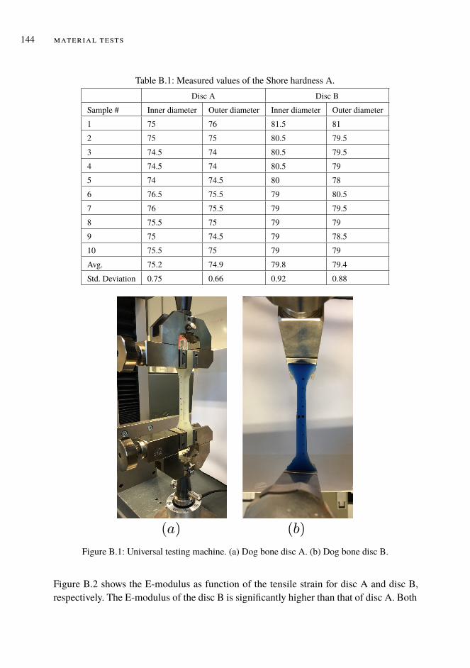
144 material tests
App
endi
xA
Table B.1: Measured values of the Shore hardness A.Disc A Disc B
Sample # Inner diameter Outer diameter Inner diameter Outer diameter1 75 76 81.5 812 75 75 80.5 79.53 74.5 74 80.5 79.54 74.5 74 80.5 795 74 74.5 80 786 76.5 75.5 79 80.57 76 75.5 79 79.58 75.5 75 79 799 75 74.5 79 78.510 75.5 75 79 79Avg. 75.2 74.9 79.8 79.4Std. Deviation 0.75 0.66 0.92 0.88
Figure B.1: Universal testing machine. (a) Dog bone disc A. (b) Dog bone disc B.
Figure B.2 shows the E-modulus as function of the tensile strain for disc A and disc B,respectively. The E-modulus of the disc B is significantly higher than that of disc A. Both
[ January 15, 2020 at 7:46 – classicthesis version 2.2 ]
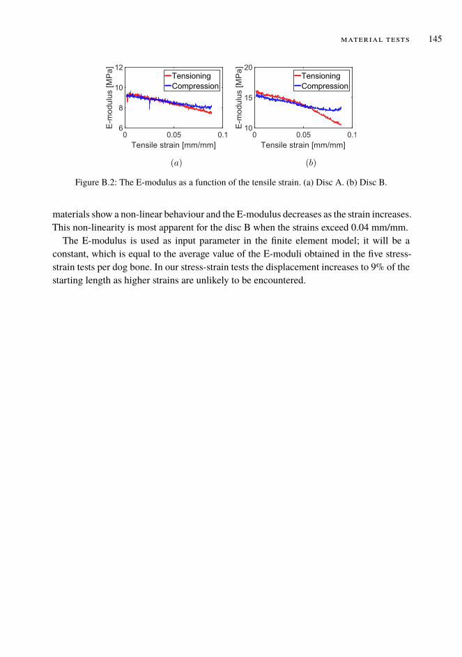
Appendix
A
material tests 145
Figure B.2: The E-modulus as a function of the tensile strain. (a) Disc A. (b) Disc B.
materials show a non-linear behaviour and the E-modulus decreases as the strain increases.This non-linearity is most apparent for the disc B when the strains exceed 0.04 mm/mm.
The E-modulus is used as input parameter in the finite element model; it will be aconstant, which is equal to the average value of the E-moduli obtained in the five stress-strain tests per dog bone. In our stress-strain tests the displacement increases to 9% of thestarting length as higher strains are unlikely to be encountered.
[ January 15, 2020 at 7:46 – classicthesis version 2.2 ]

[ January 15, 2020 at 7:46 – classicthesis version 2.2 ]

Appendix
A
CDER IVAT ION OF AN ANALYT IC SOLUT ION TO THES IMPL I F I ED MODEL
When substituting in the equation for seq (equation 4.8) into equation 4.11 we find:
p∗
ρ∗m
(Apout + Ffric)2d2δsdt2
= −δs
M0 + Mt. (C.1)
When defining a1 and a2 as:
a1 =p∗
ρ∗m
(Apout + Ffric)2M0, (C.2)
a2 =p∗
ρ∗m
(Apout + Ffric)2M, (C.3)
we can cast equation C.1 in a more general form:
d2δsdt2
= −δs
a1 + a2t. (C.4)
A solution to equation C.4 can be found by using Bessel functions:
δs(t) = C1kJ1(2k) −C2kY1(2k), (C.5)
with
k(t) =
√a1 + a2t
a22. (C.6)
Here J1 is the Bessel function of the first kind with order 1 and Y1 is the Bessel functionof the second kind with order 1.C1 andC2 are integration constants. A solution for δv(t)can be obtained by differentiating equation C.5:
δv(t) =1
a2(C1J0(2k) −C2Y0(2k)) . (C.7)
147
[ January 15, 2020 at 7:46 – classicthesis version 2.2 ]

148 derivation of an analytic solution to the simplified model
App
endi
xA
Here J0 is the Bessel function of the first kind with order 0 and Y0 is the Bessel function ofthe second kind with order 0. We now substitute the values of a1 and a2 into equation C.6to obtain:
k(t) =
√a1 + a2t
a22=
√1
a1 + a2t
(a1a2
+ t
)=
√(Apout + Ffric)2
p∗
ρ∗m(M0 + Mt)
(M0
M+ t
).
(C.8)
When using the definition for seq, equation 4.8, and subsequently the definition of thelocal angular frequencyω, equation 4.14, we can further simplify equation C.8 and arriveat equation 4.13:
k(t) =
√(Apout + Ffric)
seq(t)m
(M0
M+ t
)= ω(t)
(M0
M+ t
). (C.9)
Similarly, we can rewrite equation C.7 to obtain equation 4.15:
δv(t) =1
a1 + a2t
a1 + a2t
a2(C1J0(2k) −C2Y0(2k))
= ω2(t)
(M0
M+ t
)(C1J0(2k) −C2Y0(2k)) . (C.10)
[ January 15, 2020 at 7:46 – classicthesis version 2.2 ]

Appendix
A
DTWO-FLU ID MODEL DETA ILS
d.1 geometry
Referring to the simulations described in chapter 5 and 6, the following geometric iden-tities are used to express the wall perimeters, interfacial perimeter, and liquid height interms of the wetted angle γl:
Pgl = D sinγl, (D.1)Pl = Dγl, (D.2)Pg = D (π− γl) , (D.3)
h =1
2D (1− cosγl) . (D.4)
We use Biberg’s approximation [10] to express αl in terms of γl (this avoids the iterativesolution of a nonlinear equation):
γl = παl +
(3π
2
) 13(1− 2αl +α
13
l −α13g
). (D.5)
Figure D.1: Stratified flow layout and definitions.
149
[ January 15, 2020 at 7:46 – classicthesis version 2.2 ]
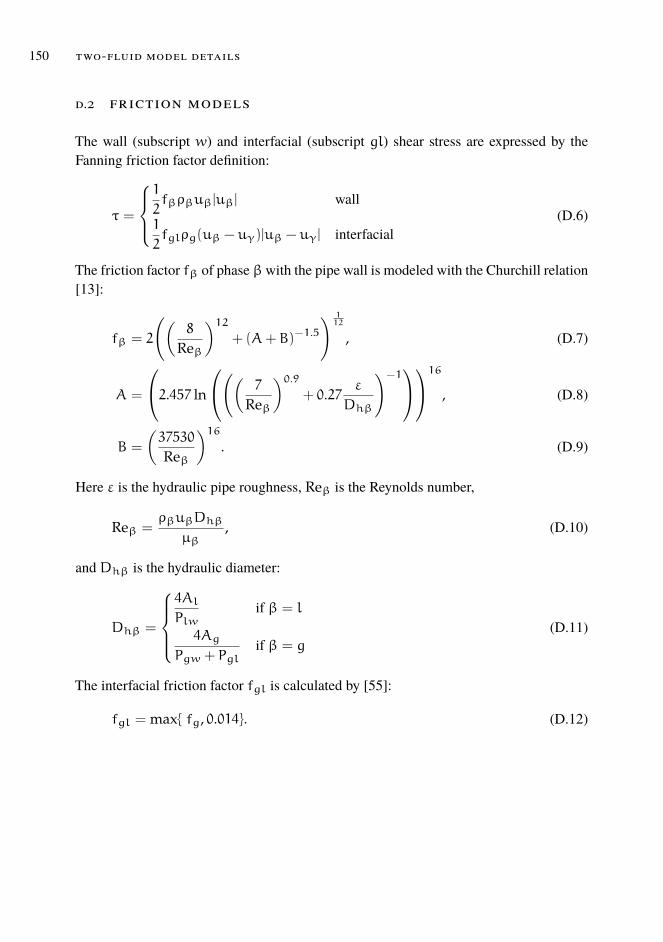
150 two-fluid model details
App
endi
xA
d.2 friction models
The wall (subscript w) and interfacial (subscript gl) shear stress are expressed by theFanning friction factor definition:
τ =
1
2fβρβuβ|uβ| wall
1
2fglρg(uβ − uγ)|uβ − uγ| interfacial
(D.6)
The friction factor fβ of phase βwith the pipe wall is modeled with the Churchill relation[13]:
fβ = 2
((8
Reβ
)12+ (A+B)−1.5
) 112
, (D.7)
A =
2.457 ln
(( 7
Reβ
)0.9
+ 0.27ε
Dhβ
)−116, (D.8)
B =
(37530
Reβ
)16. (D.9)
Here ε is the hydraulic pipe roughness, Reβ is the Reynolds number,
Reβ =ρβuβDhβ
µβ, (D.10)
and Dhβ is the hydraulic diameter:
Dhβ =
4AlPlw
if β = l
4Ag
Pgw + Pglif β = g
(D.11)
The interfacial friction factor fgl is calculated by [55]:
fgl = max fg, 0.014. (D.12)
[ January 15, 2020 at 7:46 – classicthesis version 2.2 ]
References
REFERENCES
[1] Central Intelligence Agency. The world Factbook - Country Comparison to theWorld. https://www.cia.gov/library/publications/the-world-factbook/fields/2117.html.Retrieved July 12, 2019.
[2] A. H. Akselsen. “A linear stability analyses of discrete representations of the two-fluid model for stratified two-phase flow.” In: ICMF - 9th International Confer-ence on Multiphase Flow, 2016, Firenze, Italy.
[3] A. H. Akselsen. “Efficient Numerical Methods for Waves in One-DimensionalTwo-Phase Pipe Flows.” PhD thesis. NTNU, 2016.
[4] J. E. Azpiroz. “CFD modelling of by-pass pigs.” MSc thesis. Delft University ofTechnology, 2014.
[5] J. E. Azpiroz, M. H. W. Hendrix, W.-P. Breugem, and R. A. W. M. Henkes. “CFDmodelling of bypass pigs with a deflector disk.” In: 17th Int. Conf. on MultiphaseTechnology (2015), pp. 141–155.
[6] D. Barnea and Y. Taitel. “Kelvin-Helmholtz stability criteria for stratified flow:viscous versus non-viscous (inviscid) approaches.” In: International Journal ofMultiphase Flow 19.4 (1993), pp. 639–649.
[7] D. Barnea and Y. Taitel. “Interfacial and structural stability of separated flow.” In:International Journal of Multiphase Flow 20.94 (1994), pp. 387–414.
[8] K. Bendiksen, D. Malnes, R. Moe, and S. Nuland. “The dynamic two-fluid modelOLGA. Theory and application.” In: SPE Production Engineering 6.2 (1991),pp. 171–180.
[9] R. A. Berry, L. Zou, H. Zhao, H. Zhang, J. W. Peterson, R. C. Martineau, S. Y.Kadioglu, and D. Andrs. RELAP-7 Theory manual - INL/EXT-14-31366. 2015.
[10] D. Biberg. “An explicit approximation for the wetted angle in two-phase strati-fied pipe flow.” In: The Canadian Journal of Chemical Engineering 77.3 (1999),pp. 1221–1224.
[11] J. C. Butcher. Numerical Methods for Ordinary Differential Equations. John Wi-ley & Sons, Ltd., 2003. isbn: 9780470868270.
[12] M. H. P. Carvalho and E. Rotava. “Planning and Execution of Pigging Procedurefor Gas Pipeline.” In: Offshore Technology Conference 28063 (2017), pp. 1–8.
[13] S. W. Churchill. “Friction-factor equation spans all fluid flow regimes.” In: Chem.Eng. 84 (24) (1977), pp. 91–92.
151
[ January 15, 2020 at 7:46 – classicthesis version 2.2 ]
152 references
Refe
renc
es
[14] J. Cordell. Conventional pigs - what to use and why. Pipes and Pipelines Interna-tional. 1992.
[15] J. Cordell and H. Vanzant. The pipeline pigging handbook. 3rd. ISBN: 0-9717945-3-7. Clarion Technical Publishers & Scientific Surveys Ltd., 2003.
[16] T. J. Danielson, K. M. Bansal, R. Hansen, and E. Leporcher. “LEDA: the nextmultiphase flow performance simulator.” In: BHR Group 2005 Multiphase Pro-duction Technology 12. 2005, pp. 477–492.
[17] R. Davidson. An introduction to pipeline pigging. Gulf Professional Publishing,1995.
[18] P. G.Drazin. Introduction toHydrodynamic Stability. CambridgeUniversity Press,2002.
[19] D. A. Drew and S. L. Passman. Theory ofMulticomponents Fluids. Springer, 1998.isbn: 0387983805.
[20] F.-J. Elmer. “Nonlinear dynamics of dry friction.” In: Journal of Physics A: Math-ematical and General 30.17 (1997), pp. 6057–6063.
[21] A. Entaban, A. Ismail, M. Jambari, P. Ting, K. M. Amin, C. Ping, S. Zou, and G.van Spronsen. “By-Pass pigging - A ’simple’ technology with significant businessimpact.” In: Society of Petroleum Engineers - International Petroleum TechnologyConference 2013, IPTC 2013. Vol. 5. 2013, pp. 3666–3671.
[22] F. Esmaeilzadeh, D. Mowla, and M. Asemani. “Mathematical modeling and sim-ulation of pigging operation in gas and liquid pipelines.” In: Journal of PetroleumScience and Engineering 69.1-2 (2009), pp. 100–106.
[23] A. B. Figueiredo, R. M. Baptista, F. B. D. Freitas Rachid, and G. C. R. Bodstein.“Numerical simulation of stratified-pattern two-phase flow in gas pipelines using atwo-fluid model.” In: International Journal of Multiphase Flow 88 (2017), pp. 30–49.
[24] Fluent Theory Guide. 14th ed. Ansys Inc.
[25] W. D. Fullmer, V. H. Ransom, andM. A. Lopez de Bertodano. “Linear and nonlin-ear analysis of an unstable, but well-posed, one-dimensional two-fluid model fortwo-phase flow based on the inviscid Kelvin-Helmholtz instability.” In: NuclearEngineering and Design 268 (2014), pp. 173–184.
[26] A. Gent. “On the relation between indentation hardness and Young’s modulus.”In: Rubber Chemistry and Technology 31.4 (1958), pp. 896–906.
[27] H. Goedecke. “Ultrasonic or MFL Inspection: Which Technology Is Better forYou?” In: Pipeline and Gas Journal 230 (Oct. 2003), pp. 34–41.
[ January 15, 2020 at 7:46 – classicthesis version 2.2 ]

References
references 153
[28] A. Goldszal, J. I. Monsen, T. J. Danielson, K. M. Bansal, Z. L. Yang, S. T. Jo-hansen, and G. Depay. “LedaFlow 1D: Simulation results with multiphase gas/-condensate and oil/gas field data.” In: 13th International Conference on Multi-phase Production Technology (2007), pp. 17–31.
[29] C. M. Graafland. “Frictional behaviour of pigs.” MSc thesis. Delft University ofTechnology, 2017.
[30] G. A. Groote, P. B. J. van de Camp, P. Veenstra, G. Broze, and R. A.W.M. Henkes.“By-pass pigging without or with speed control for gas-condensate pipelines.” In:Society of Petroleum Engineers - Abu Dhabi International Petroleum Exhibitionand Conference, ADIPEC 2015. 2015.
[31] E. Hairer, S.P. Norsett, and G. Wanner. Solving Ordinary Differential EquationsI. Springer, 2008. isbn: 978-3-540-56670-0.
[32] A. den Heijer. “Frictional behaviour of pigs in motion.” MSc thesis. Delft Univer-sity of Technology, 2016.
[33] M. H. W. Hendrix, I. E. Smith, J. S. B. van Zwieten, and B. Sanderse. “Compari-son of numerical methods for slug capturing with the two-fluid model.” In: ICMF- 9th International Conference on Multiphase Flow 2016, Firenze, Italy. 2016.
[34] M. H. W. Hendrix, A. den Heijer, W.-P. Breugem, and R. A. W. M. Henkes. “Fric-tional forces during pigging of multiphase pipelines.” In: BHRGroup - 10th NorthAmerican Conference on Multiphase Technology 2016 (2016), pp. 103–114.
[35] M. H. W. Hendrix, X. Liang, W.-P. Breugem, and R. A. W. M. Henkes. “Char-acterization of the pressure loss coefficient using a building block approach withapplication to by-pass pigs.” In: Journal of Petroleum Science and Engineering150 (2017), pp. 13–21.
[36] M. H. W. Hendrix, H. P. IJsseldijk, W.-P. Breugem, and R. A. W. M. Henkes.“Development of speed controlled pigging for low pressure pipelines.” In: 18thInternational Conference onMultiphase Production Technology,MPT 2017 2017-June (2017), pp. 501–509.
[37] M. H. W. Hendrix, H. P. IJsseldijk, W.-P. Breugem, and R. A. W. M. Henkes.“Experiments and modelling of by-pass pigging under low pressure conditions.”In: Journal of Process Control 17 (2018), pp. 1–13.
[38] M. H. W. Hendrix, H. P. IJsseldijk, W.-P. Breugem, and R. A. W. M. Henkes.“Simulation of slug propagation for by-pass pigging in two-phase stratified pipeflow.” In: 19th Int. Conf. on Multiphase Technology (2019), pp. 317–330.
[39] R. A. W. M. Henkes. Guidelines for the Hydraulic Design and Operation of Mul-tiphase Flow Pipeline Systems. Shell Global Solutions, 2019.
[40] C. Hirsch. Numerical Computation of Internal and External Flows - Volume I,Fundamentals of Numerical Discretization. Wiley, 1994.
[ January 15, 2020 at 7:46 – classicthesis version 2.2 ]

154 references
Refe
renc
es
[41] H.Holmås. “Numerical simulation of transient roll-waves in two-phase pipe flow.”In: Chemical Engineering Science 65.5 (2010), pp. 1811–1825.
[42] S. M. Hosseinalipour, A. Zarif Khalili, and A. Salimi. “Numerical simulation ofpig motion through gas pipelines.” In: 16th Australasian Fluid Mechanics Con-ference. 2007, pp. 971–975.
[43] W. Hundsdorfer and J. Verwer.Numerical Solution of Time-Dependent Advection-Diffusion-Reaction Equations. Vol. 33. Springer, 2007. isbn: 978-3-642-05707-6.
[44] H. P. IJsseldijk. “By-pass pigging - Experiments and simulations.” MSc thesis.Delft University of Technology, 2016.
[45] I. E. Idelchik.Handbook of Hydraulic Resistance. 2nd ed. Hemisphere PublishingCorporation, 1987.
[46] R. I. Issa and M. H. W. Kempf. “Simulation of slug flow in horizontal and nearlyhorizontal pipes with the two-fluid model.” In: International Journal of Multi-phase Flow 29.1 (2003), pp. 69–95.
[47] B. Jamshidi and M. Sarkari. “Simulation of pigging dynamics in gas-liquid two-phase flow pipelines.” In: Journal of Natural Gas Science and Engineering 32(2016), pp. 407–414.
[48] G. W. Johnson. “A Study of Stratified Gas-Liquid Pipe Flow.” PhD thesis. Uni-versity of Oslo, 2005.
[49] J. Kjølaas, A. De Leebeeck, and S. T. Johansen. “Simulation of hydrodynamicslug flow using the LedaFlow slug capturing model.” In: 16th International Con-ference onMultiphase Production Technology, 12-14 June, Cannes, France (2013).
[50] K. Kohda, Y. Suzukawa, and H. Furukawa. “New method for analyzing transientflow after pigging scores well.” In: Oil and Gas Journal 86.19 (1988), pp. 40–47.
[51] P. K. Kundu, L.M. Cohen, and D. R. Dowling.Fluid mechanics. 5th ed. AcademicPress, 2012.
[52] Z. Lan, S. Liu, H. Xiao, and D. Wang. “Frictional Behavior of Wax–Oil GelsAgainst Steel.” In: Tribology Letters 65.3 (2017), p. 88.
[53] H. S. Lee, D. Agustiawan, K. Jati, M. A. H. Aulia, S. A. Thomas, and S. P. Ap-pleyard. “By-pass pigging operation experience and flow assurance study.” In:Offshore Technology Conference (2012), pp. 1–10.
[54] X. Liang. “Numerical study of flow around by-pass pigs.” MSc thesis. Delft Uni-versity of Technology, 2015.
[55] J. Liao, R. Mei, and J. F. Klausner. “A study on the numerical stability of thetwo-fluidmodel near ill-posedness.” In: International Journal of Multiphase Flow34.11 (2008), pp. 1067–1087.
[ January 15, 2020 at 7:46 – classicthesis version 2.2 ]

References
references 155
[56] H. Liu. Pipeline Engineering. ISBN: 0-58716-140-0. Lewis Publishers, 2003.
[57] R. W. Lyczkowski, D. Gidaspow, C. W. Solbrig, and E. D. Hughes. “Characteris-tics and stability analyses of transient one-dimensional two-phase flow equationsand their finite difference approximations.” In: Nuclear Science and Engineering66.3 (1978), pp. 378–396.
[58] C. M. Graafland M. H. W. Hendrix and R. van Ostayen. “Frictional forces duringpipeline pigging.” In: Journal of Petroleum Science and Engineering 171 (2018),pp. 905–918.
[59] J. M.Masella, Q. H. Tran, D. Ferre, and C. Pauchon. “Transient simulation of two-phase flows in pipes.” In: International Journal of Multiphase Flow 24.5 (1998),pp. 739–755.
[60] B. S. Massey. Mechanics of Fluids. 9th ed. Spon Press, 2012.
[61] K. Minami and O. Shoham. “Pigging dynamics in two-phase flow pipelines: Ex-periment and modeling.” In: SPE Production and Facilities 10.4 (1995), pp. 225–231.
[62] M. Mirshamsi and M. Rafeeyan. “Speed control of pipeline pig using the QFTmethod.” In: Oil and Gas Science Technology 67.4 (2012), pp. 693–701.
[63] N. Money, D. Cockfield, S. Mayo, and G. Smith. “Dynamic speed control in highvelocity pipelines.” In: Pipeline and Gas Journal 239(8) (2012), pp. 30–38.
[64] M.Montini. “Closure Relations of the One-Dimensional Two-Fluid Model for theSimulation of Slug Flows.” PhD thesis. Imperial College, 2011.
[65] A. Morin, T. Flåtten, and S. T. Munkejord. “A Roe scheme for a compressiblesix-equation two-fluid model.” In: International Journal for Numerical Methodsin Fluids 72 (2013), pp. 478–504. doi: 10.1002/fld.
[66] K.W.Morton and D.Mayers.Numerical Solution of Partial differential Equations.Cambridge University Press, 2005. isbn: 9780521607933.
[67] T. T. Nguyen, S. B. Kim, H. R. Yoo, and Y. W. Rho. “Modeling and simulationfor PIG with bypass flow control in natural gas pipeline.” In: KSME InternationalJournal 15.9 (2001), pp. 1302–1310.
[68] T. T. Nguyen, H. R. Yoo, Y. W. Rho, and S. B. Kim. “Speed control of pig us-ing bypass flow in natural gas pipeline.” In: IEEE International Symposium onIndustrial Electronics 2 (2001), pp. 863–868.
[69] A. O. Nieckele, A. M. B. Braga, and L. F. A. Azevedo. “Transient pig motionthrough gas and liquid pipelines.” In: Journal of Energy Resources Technology,Transactions of the ASME 123.2-4 (2001), pp. 260–268.
[70] A. F. O’Donoghue. “On the steady motion of conventional pipeline pigs usingincompressible drive media.” PhD thesis. Cranfield University, 1996.
[ January 15, 2020 at 7:46 – classicthesis version 2.2 ]

156 references
Refe
renc
es
[71] R. Olsen. “Time Dependent Boundary Conditions for Multiphase Flow.” PhDthesis. NTNU, 2004.
[72] B. N. J. Persson. Sliding Friction. ISBN: 3-540-63296-4. Springer, 1998.
[73] A. Prosperetti and G. Tryggvason. Computational Methods for Multiphase Flow.Cambridge University Press, 2007. isbn: 9780521847643.
[74] J. Quarini and S. Shire. “A review of fluid-driven pipeline pigs and their applica-tions.” In: Journal of Process Mechanical Engineering 221.1 (2007), pp. 1–10.
[75] C. Ramella et al. “A novel smart caliper foam pig for low-cost pipeline inspection- Part B: Field test and data processing.” English. In: Journal of Petroleum Scienceand Engineering 133 (2015), pp. 771–775.
[76] J. D. Ramshaw and J. A. Trapp. “Characteristics, stability, and short-wavelengthphenomena in two-phase flow equation systems.” In: Nuclear Science and Engi-neering 66 (1978), pp. 93–102.
[77] B.W. Righolt, S. Kenjereš, R. Kalter,M. J. Tummers, and C. R. Kleijn. “Dynamicsof an oscillating turbulent jet in a confined cavity.” In: Physics of Fluids 27 (2015).
[78] Z. Rui, G. Han, H. Zhang, S. Wang, H. Pu, and K. Ling. “A new model to eval-uate two leak points in a gas pipeline.” In: Journal of Natural Gas Science andEngineering 46.36 (2017), pp. 491–497.
[79] Z. Rui, X. Wang, Z. Zhang, J. Lu, G. Chen, X. Zhou, and S. Patil. “A realistic andintegrated model for evaluating oil sands development with Steam Assisted Grav-ity Drainage technology in Canada.” In: Applied Energy 213.7 (2018), pp. 76–91.
[80] B. Sanderse, I. E. Smith, and M. H. W. Hendrix. “Analysis of time integrationmethods for the compressible two-fluid model for pipe flow simulations.” In: In-ternational Journal of Multiphase Flow 95 (2017), pp. 155–174.
[81] H. J. Sheen, W. J. Chen, and J. S. Wu. “Flow patterns for an annular flow overan axisymmetric sudden expansion.” In: Journal of Fluid Mechanics 350 (1997),pp. 177–188.
[82] A. Singh and R. A. W. M. Henkes. “CFD modelling of the flow around a by-pass pig.” In: 8th North American Conference on Multiphase Technology (2012),pp. 229–243.
[83] H. B. Stewart and B. Wendroff. “Two-phase flow: models and methods.” In: Jour-nal of Computational Physics 56 (1984), pp. 363–409.
[84] G.-B. Tan, D.-G. Wang, S.-H. Liu, and S.-W. Zhang. “Frictional behaviors ofrough soft contact on wet and dry pipeline surfaces:With application to deepwaterpipelaying.” In: Science China Technological Sciences 56 (2013), pp. 3024–3032.
[ January 15, 2020 at 7:46 – classicthesis version 2.2 ]
References
references 157
[85] G.-B. Tan, D.-G. Wang, S.-H. Liu, and S.-W. Zhang. “Probing tribological prop-erties of waxy oil in pipeline pigging with fluorescence technique.” In: TribologyInternational 71 (2014), pp. 26–37.
[86] G.-B. Tan, S.-H. Liu, D.-G. Wang, and S.-W. Zhang. “Spatio-temporal structurein wax-oil gel scraping at a soft tribological contact.” In: Tribology International88 (2015), pp. 236–251.
[87] R. G. Teyssandier and M. P. Wilson. “An analysis of flow through sudden enlarge-ments in pipes.” In: Journal of Fluid Mechanics 64.1 (1974), pp. 85–95.
[88] K.W. Thompson. “Time dependent boundary conditions for hyperbolic systems.”In: Journal of Computational Physics 68.1 (1987), pp. 1–24.
[89] U. Thuenemann and J.Wegjan-Kuipers. “Control your speed.” In:World Pipelines3(3) (2003), pp. 31–32.
[90] J. N. H. Tiratsoo. Pipeline pigging technology. 2nd. ISBN: 0-8720142-6-6. GulfProfessional Publishing, 1992.
[91] S. T. Tolmasquim and A. O. Nieckele. “Design and control of pig operationsthrough pipelines.” In: Journal of Petroleum Science and Engineering 62.3-4(2008), pp. 102–110.
[92] M. J. Tummers, A. W. Hübner, E. H. van Veen, K. Hanjalić, and Th H. van derMeer. “Hysteresis and transition in swirling nonpremixed flames.” In:Combustionand Flame 156.2 (2009), pp. 447–459.
[93] K. P. Vanoverberghe, E. V. van den Bulck, and M. J. Tummers. “Confined annularswirling jet combustion.” In: Combustion Science and Technology 175.3 (2003),pp. 545–578.
[94] Q. Wang, C. Sarica, and M. Volk. “An experimental study on wax removal inpipes with oil flow.” In: Journal of Energy Resources Technology, Transactionsof the ASME 130.4 (2008), pp. 0430011–0430015.
[95] M. White, K. Pierce, and T. Acharya. “A Review of Wax-Formation/MitigationTechnologies in the Petroleum Industry.” In: Society of PetroleumEngineers 189447(2017), pp. 1–10.
[96] H. L. Wu and G. van Spronsen. “Slug reduction with high by-pass pigs - a maturetechnology.” In: 12th International Conference on Multiphase Production Tech-nology, Barcelona (2005), pp. 313–325.
[97] X.-X.Xu and J. Gong. “Pigging simulation for horizontal gas-condensate pipelineswith low-liquid loading.” In: Journal of Petroleum Science and Engineering 48.3-4 (2005), pp. 272–280.
[ January 15, 2020 at 7:46 – classicthesis version 2.2 ]

158 references
Refe
renc
es
[98] H. Zhang, C. Sanchez, S. Liu, S. Zhang, and H. Liang. “Wear of a polyurethanerubber used in dry gas pipeline as inspection gauges.” In: Journal of Natural GasScience and Engineering 41 (2017), pp. 40–48.
[99] X. Zhu, D.Wang, H. Yeung, S. Zhang, and S. Liu. “Comparison of linear and non-linear simulations of bidirectional pig contact forces in gas pipelines.” In: Journalof Natural Gas Science and Engineering 27 (2015), pp. 151–157.
[100] X. Zhu, S. Zhang, X. Li, D. Wang, and D. Yu. “Numerical simulation of con-tact force on bi-directional pig in gas pipeline: At the early stage of pigging.” In:Journal of Natural Gas Science and Engineering 23 (2015), pp. 127–138.
[101] X. Zhu,W.Wang, S. Zhang, and S. Liu. “Experimental Research on the FrictionalResistance of Fluid-Driven Pipeline Robot with Small Size in Gas Pipeline.” In:Tribology Letters 65.2 (2017).
[102] L. Zou, H. Zhao, andH. Zhang. “Applications of high-resolution spatial discretiza-tion scheme and Jacobian-free Newton-Krylov method in two-phase flow prob-lems.” In: Annals of Nuclear Energy 83 (2015), pp. 101–107.
[103] J. S. B. van Zwieten, B. Sanderse, M. H. W. Hendrix, C. Vuik, and R. A. W. M.Henkes. Efficient simulation of one-dimensional two-phase flow with a new high-order Discontinuous Galerkin method, Report 15-07. Tech. rep. Delft Universityof Technology, 2015.
[ January 15, 2020 at 7:46 – classicthesis version 2.2 ]
References
ACKNOWLEDGMENTS
First of all I would like to thank my promotor Ruud Henkes for giving me the opportunityto embark on this exciting project. The combination of fundamental research with a clearpractical application provided an interesting project to work on. You helped me to applythe right focus to take all the steps that are needed to finish a PhD project: from writingup the very first results in a paper, to keeping me motivated until the very end when I waswriting the draft of this thesis. I also would like to thank you for the very fast and detailedfeedback on my draft papers and thesis chapters, which usually took no longer than a dayor two!
I would like to thankmy daily supervisor and promotorWim-Paul Breugem.You alwaystake enough time during scientific discussions to thoroughly analyze a problem to the verycore. This is a quality that I greatly appreciated inworking together. I also enjoyed assistingin the turbulence course that you lectured - a course that is very well received by students.I quickly understood why!I would like to thank both my promotors for having the patience with me to complete all
the chapters and papers which are part of this thesis. I want to emphasize that I appreciatethe constructive and inspiring conversations we have had, which have led to the sharpeningand completion of this thesis.During my PhD I had the pleasure to share an office with Andries and Daniele, and later
on also Tariq. Thanks for the fun moments we have had! I also would like to thank all otherlab members for providing a very nice working environment. In particular I enjoyed theChristmas festivities and of course the group outings that were organized by the laboratory.I would also like to thank the GoT group for many very well organized movie nights!The PhD project has been carried out in collaboration with Shell. I regularly visited
Shell Technology Centre Amsterdam. I would like to thank Peter Veenstra, who wasclosely involved during the course of this project and has continuously provided valuablepractical feedback. Also I would like to give a big thanks to the involvement of variouspeople from the Flow Assurance team in Shell. In particular, I would like to thank Ben-jamin Sanderse. Our paths crossed early on and it was a pleasure to work on our jointpublications. I learnt a lot from your rigorous mathematical approach, and your two-fluidmodel solver was the starting point for the numerical simulations that led to the resultsof chapter 5 and 6. Also I would like to thank Gijs Groote and Maurice Fransen for theirinvolvement regarding the practical implications of this work.I would like to thank Ivar Smith and Joost van Zwieten for pleasant collaboration on
our joint publications.I want to thank Caroline for all the administrative support during my PhD.
159
[ January 15, 2020 at 7:46 – classicthesis version 2.2 ]

160 references
Refe
renc
es
I have had the pleasure to work with five master students: Javier, Xiaoyun, Arie, Harm,Chris, your work has all contributed to this thesis and I am grateful for that. I also had thepleasure to work with four bachelor students for their final project. Your project stood out,as it had created some very visible results. Thanks, Daan, Luuk, Sytse, and Tim! I wouldlike to thank Jasper and Jan for supporting the experiments which were part of the studentprojects.A final word of gratitude goes to my family and friends and my girlfriend Roza for their
continuous support!
Maurice HendrixDelft, August 2019
[ January 15, 2020 at 7:46 – classicthesis version 2.2 ]

References
CURR ICULUM VITÆ
personal information
full name: Maurice Hans Willem Hendrix
birth date: 30 September 1988
nationality: Dutch
education and employment
2017-now: Instrumentation Engineer, Shell Pernis, The Netherlands.
2013-2017: PhD Researcher in the Laboratory for Hydro & Aerodynamics,Process & Energy Department, Delft University of Technology, The Netherlands.
2011-2013: MSc in Applied Physics, Universiteit Twente, The Netherlands;Exchange Student, Nanyang Technological University, Singapore (in 2011, for fourmonths).
2007-2011: BSc in Applied Physics, Universiteit Twente, The Netherlands.
161
[ January 15, 2020 at 7:46 – classicthesis version 2.2 ]

[ January 15, 2020 at 7:46 – classicthesis version 2.2 ]
References
L I ST OF PUBL ICAT IONS
journal publications
[1] M.H.W. Hendrix, H.P. IJsseldijk, W.-P. Breugem, and R.A.W.M. Henkes, "Experi-ments and modelling of by-pass pigging under low pressure conditions.", Journalof Process Control, vol. 71, pp. 1-13, 2018.
[2] M.H.W. Hendrix, C.M. Graafland, and R. van Ostayen, "Frictional forces for disc-type pigging of pipelines.", Journal of Petroleum Science and Engineering, vol. 171,pp. 905-918, 2018.
[3] B. Sanderse, I.E. Smith, and M.H.W. Hendrix, "Analysis of time integration meth-ods for the compressible two-fluid model for pipe flow simulations.", InternationalJournal of Multiphase Flow, vol. 95, pp. 155-174, 2017.
[4] M.H.W. Hendrix, X. Liang, W.-P. Breugem, and R.A.W.M. Henkes, "Characteriza-tion of the pressure loss coefficient using a building block approach with applicationto by-pass pigs.", Journal of Petroleum Science and Engineering, vol. 150, pp. 13-21, 2016.
conference publications and contributions
[1] M.H.W. Hendrix, B. Sanderse,W.-P. Breugem, and R.A.W.M. Henkes, "Simulationof slug propagation for by-pass pigging in two-phase stratified pipe flow.", BHRGroup - 19th International Conference on Multiphase Technology, pp. 317-330,2019.
[2] M.H.W. Hendrix, H.P. IJsseldijk, W.-P. Breugem, and R.A.W.M. Henkes, "Devel-opment of speed controlled pigging for low pressure pipelines.", BHR Group - 18thInternational Conference on Multiphase Technology, pp. 501-509, 2017.
[3] M.H.W. Hendrix, A. den Heijer,W.-P. Breugem, and R.A.W.M. Henkes, "Frictionalforces during pigging of multiphase pipelines.", BHRGroup - 10th North AmericanConference on Multiphase Technology, pp. 103-114, 2016.
[4] J.E. Azpiroz, M.H.W. Hendrix, W.-P. Breugem, and R.A.W.M. Henkes, "CFDmod-elling of bypass pigs with a deflector disk.", BHR Group - 17th International Con-ference on Multiphase Technology, pp. 141-158, 2015.
163
[ January 15, 2020 at 7:46 – classicthesis version 2.2 ]

164 references
Refe
renc
es
journal publications outside this thesis
[1] J.S.B van Zwieten, B. Sanderse, M.H.W. Hendrix, C. Vuik, and R.A.W.M. Henkes,"Efficient simulation of one-dimensional two-phase flowwith a high-order h-adaptivespace-time Discontinuous Galerkin method.", Computer and Fluids, vol. 156, pp.34-47, 2017.
[2] M.H.W. Hendrix,W. Bouwhuis, D. van derMeer, D. Lohse, and J.H. Snoeijer, "Uni-versal mechanism for air entrainment during liquid impact.", Journal of Fluid Me-chanics, vol. 789, pp. 708-725, 2016.
[3] W. Bouwhuis, M.H.W. Hendrix, D. van der Meer, and J.H. Snoeijer, "Initial surfacedeformations during impact on a liquid pool.", Journal of FluidMechanics, vol. 771,pp. 503-519, 2015.
[4] E. Klaseboer, R. Manica, M.H.W. Hendrix, C.-D. Ohl, and D.Y.C. Chan, "A forcebalance model for the motion, impact, and bounce of bubbles.", Physics of Fluids,vol. 26, pp. 092101-01 - 092101-12, 2014.
[5] R. Manica, M.H.W. Hendrix, R. Gupta, E. Klaseboer, C.-D. Ohl, and D.Y.C. Chan,"Modelling bubble rise and interactionwith a glass surface.",AppliedMathematicalModelling, vol. 38, pp. 4249-4261, 2014.
[6] R.C.A. van der Veen, M.H.W. Hendrix, T. Tran, C. Sun, P.A. Tsai, and D. Lohse,"How microstructures affect air film dynamics prior to drop impact.", Soft Matter,vol. 10, pp. 3703-3707, 2014.
[7] R. Manica, M.H.W. Hendrix, R. Gupta, E. Klaseboer, C.-D. Ohl, and D.Y.C. Chan,"Effect of film hydrodynamic boundary condition on bubble-wall impact.", SoftMatter, vol. 9, pp. 9755-9758, 2013.
[8] M.H.W. Hendrix, R. Manica, E. Klaseboer, D.Y.C. Chan, and C.-D. Ohl, "Spa-tiotemporal evolution of thin liquid films during impact of water bubbles on glass ona micrometer to nanometer scale.", Physical Review Letters, vol. 108, pp. 247803-01 - 247803-04, 2012.
[9] P.A. Tsai, M.H.W. Hendrix, R.R.M. Dijkstra, L. Shui, and D. Lohse, "Microscopicstructure influencing macroscopic splash at high Weber number.", Soft Matter, vol.7, pp. 11325-11333, 2011.
[ January 15, 2020 at 7:46 – classicthesis version 2.2 ]