EXPERIMENTS AND MODEL DEVELOPMENT OF A DUAL MODE ...

EXPERIMENTS AND MODEL DEVELOPMENT OF A DUAL

MODE, TURBULENT JET IGNITION ENGINE

By

Sedigheh Tolou

A DISSERTATION

Submitted to

Michigan State University

in partial fulfillment of the requirements

for the degree of

Mechanical Engineering—Doctor of Philosophy

2019

ABSTRACT

EXPERIMENTS AND MODEL DEVELOPMENT OF A DUAL MODE, TURBULENT JET

IGNITION ENGINE

By

Sedigheh Tolou

The number of vehicles powered by a source of energy other than traditional petroleum fuels will

increase as time passes. However, based on current predictions, vehicles run on liquid fuels will

be the major source of transportation for decades to come. Advanced combustion technologies can

improve fuel economy of internal combustion (IC) engines and reduce exhaust emissions. The

Dual Mode, Turbulent Jet Ignition (DM-TJI) system is an advanced, distributed combustion

technology which can achieve high diesel-like thermal efficiencies at medium to high loads and

potentially exceed diesel efficiencies at low-load operating conditions. The DM-TJI strategy

extends the mixture flammability limits by igniting lean and/or highly dilute mixtures, leading to

low-temperature combustion (LTC) modes in spark ignition (SI) engines.

A novel, reduced order, and physics-based model was developed to predict the behavior of a DM-

TJI engine with a pre-chamber air valve assembly. The engine model developed was calibrated

based on experimental data from a Prototype II DM-TJI engine. This engine was designed, built,

and tested at the MSU Energy and Automotive Research Laboratory (EARL).

A predictive, generalized model was introduced to obtain a complete engine fuel map for the DM-

TJI engine. The engine fuel map was generated in a four-cylinder boosted configuration under

highly dilute conditions, up to 40% external exhaust gas recirculation (EGR).

A vehicle simulation was then performed to further explore fuel economy gains using the fuel map

generated for the DM-TJI engine. The DM-TJI engine was embodied in an industry-based vehicle

to examine the behavior of the engine over the U.S. Environmental Protection Agency (EPA)

driving schedules. The results obtained from the drive cycle analysis of the DM-TJI engine in an

industry-based vehicle were compared to the results of the same vehicle with its original engine.

The vehicle equipped with the DM-TJI system was observed to benefit from ~13% improvement

in fuel economy and ~11% reduction in CO2 emission over the EPA combined city/high driving

schedules. Potential improvements were discussed, as these results of the drive cycle analysis are

the first-ever reported results for a DM-TJI engine embodied in an industry-based vehicle.

The resulting fuel economy and CO2 emission were used to conduct a cost-benefit analysis of a

DM-TJI engine. The cost-benefit analysis followed the economic and key inputs used by the U.S.

EPA in a Proposed Determination prepared by that agency. The outcomes of the cost-benefit

analysis for the vehicle equipped with the DM-TJI system were reported in comparison with the

same vehicle with its base engine. The extra costs of a DM-TJI engine were observed to be

compensated over the first three years of the vehicle’s life time. The results projected maximum

savings of approximately 2400 in 2019 dollars. This includes the lifetime-discounted present value

of the net benefits of the DM-TJI technology, compared to the base engine examined. In this dollar

saving estimate, the societal effects of CO2 emission were calculated based on values by the

interagency working group (IWG) at 3% discount rate.

iv

To my Mother and my Father

“I am so close, I may look distant.

So completely mixed with you, I may look separate.

So out in the open, I appear hidden.

So silent, because I am constantly talking with you.”

- Rumi

v

ACKNOWLEDGEMENTS

First and foremost, I would like to acknowledge my PhD adviser Professor Harold Schock for his

continuous support over the course of last five years. Dr. Schock accepted me as his PhD student,

while my resume did not reflect much of engine-related research. He trusted my eagerness to learn

and gave me an opportunity to grow. I will be, forever, thankful for this opportunity. I found myself

and learned to trust my capabilities through his leadership. I learned from him through his

comments at various times, not only in regard to me but also when it came to others. I completely

understood that there is nothing as “my bad” and you are allowed to make “small mistakes,” as

long as you learn from them. I learned that you should find the person to trust and after that, you

should allow them to guide you in the right direction. I learned that the path may have its own ups

and downs. However, you will be fine at the end if you have chosen the right person to trust. Dr.

Schock, I am truly grateful for having you as my adviser and I will never forget the journey we

had together.

I am very grateful to Dr. Matt Brusstar of the U.S. EPA who was not officially my adviser but did

not put forward anything less than an adviser. I will never forget our first one-by-one meeting, as

he walked me through the reality of life. He taught me to raise my level of acceptance if I wish to

accomplish anything in life. He and his to-the-point comments shed light on so many of my mind

questions. When it comes to him, I will never know which one is going to win, his depth of

knowledge or his eagerness to teach. Thank you, Matt. You have been a true mentor to me.

I would like to thank Professor Thomas Voice for having served both as a member of my PhD

committee and the primary adviser for my PhD specialization in “Environmental Policy.” Dr.

Voice clearly saw my needs to define the right project which was worth the effort. I could never

vi

guess, such a blessing this experience will turn out to be. I truly enjoyed our conversations in the

realm of policy which introduced me to a completely new scenery. Dr. Voice, thank you for

believing in me.

I am grateful to my other committee members: Professor Guoming (George) Zhu for his clarifying

suggestions on combustion zone modeling and engine simulations. Dr. Zhu, your suggestions have

always rung a bell in my mind and for that and so many other things, I am truly thankful. Professor

Farhad Jaberi for having taught me three graduate courses and for having served as a member of

my PhD committee. I have always admired his depth of knowledge in model development and

numerical simulations. Dr. Jaberi, thanks for teaching me all those exciting materials.

I am wholeheartedly grateful to Thomas Stuecken for his support, always being there, and

technical knowledge. Tom could always propose a novel, exciting way for testing a phenomenon.

Tom, you have been a true friend and I have learned a lot from you. I never understood how one

person could be this much knowledgeable and, at the same time, 100-percent down-to-earth. I will

never forget our times together, Mr. Bubble!

Furthermore, I want to acknowledge Kevin Moran, Brian Rowley, John Przybyl, and Brian

Deimling for their help in setting up the experiments. I could not have finished the work if you had

not been there to help. I would also like to Thank Jennifer Higel for her wonderful depiction of

realities. Jen, thanks a lot for your prompt response and for always willingness to help. A special

thanks goes to the current and former graduate students: Dr. Ravi Teja Vedula, Dr. Ali Kharazmi,

Dr. Ruitao Song, Sabah Sadiyah Chowdhury, Cyrus Atis Arupratan, Yidnekachew Ayele, Yifan

Men, Shen Qu, Christine Li, and Prasanna Chinnathambi. Thank you all for your support. It has

been such a journey and I have learned from every one of you. Sabah, particularly thank you for

vii

all the emotional support and tolerating me crashing into your computer. I know it has been just a

few months, but you are already one of my favorites.

My PhD project was supported by the U.S. EPA, Tenneco Inc., and the State of Michigan under

Grant Number 83589201. I would like to thank Dr. Yong Sun and Adam Kotrba of Tenneco Inc.

for their technical support. I am also grateful to so many people at the U.S. EPA National Vehicle

and Fuel Emissions Laboratory (NVFEL) including: Mark Stuhldreher, Thomas Veling, Donald

Dennis, Aaron Hula, Dr. Bob Giannelli, Dr. Andrew Moskalik, Ray Kondel, and Greg Davis. I

could say something about every one of you, but it would take pages! I strongly believe that I could

not have finished the project if I had not learned from each and every one of you. Thank you, all.

I have been extremely fortunate to learn from Jeff Alson (U.S. EPA), while working on my policy

project. He has been the source to all I have learned in this regard. Jeff with his lifetime experience

and knowledge was tremendously calm and patient, as he shaped my understanding of this new

world. Thank you, Jeff.

I will be, forever, grateful for the help of Dr. Gloria Helfand (U.S. EPA). She has been a sudden

blessing in the sky. I massively enjoyed her comments and suggestions, as she reviewed my final

report of the policy project. Thank you, Gloria. You are amazing.

I want to also thank Paul Dekraker (U.S. EPA) for his help on the drive cycle analysis using the

EPA ALPHA model. My drive cycle analysis would not have been completed if you had not been

there to carefully explain every bit of details I needed to know. Thank you, Paul.

I am also thankful to my peers at UoM: Christina Reynolds, Justin Koczak, and Niket Prakash. I

truly enjoyed our monthly meetings at NVFEL. I learned from you and grew with you. A special

thanks also goes to Niket for walking me through the EPA ALPHA model. Thank you, guys!

viii

Finally, I would like to thank my family – my extended family, my in-laws, my parents, my sister,

Elaheh, my brother-in-law, Arjang, my wonderful nephew whom I miss dearly, Kian, and my

husband, Hamid – for their love and support at different stages of my studies. Elaheh, my dearest

sister, I promise I would not miss all the tea times any more. Thank you for holding my place and

not giving it up easily. I specially want to thank my parents for believing in me to pursue my

dreams. None of this would have happened if they had not gone through ups and downs of this

journey with me. Thank you, you have been, always and forever, my strongest shoulder to hold

on. Hamid, my best friend and partner in life, I have been the most fortunate to have you alongside

me through this seemed-to-be endless journey at times. Thanks for always being there, no matter

what!

vii

TABLE OF CONTENTS

LIST OF TABLES ......................................................................................................................... ix

LIST OF FIGURES ....................................................................................................................... xi

CHAPTER 1 INTRODUCTION .................................................................................................... 1

1.1 Background and Motivation ............................................................................................. 1

1.2 Structure of Dissertation................................................................................................... 5

1.3 Specific Aims ................................................................................................................... 6

CHAPTER 2 COMBUSTION MODEL FOR A HOMOGENEOUS TURBOCHARGED

GASOLINE DIRECT INJECTION ENGINE ................................................................................ 8

2.1 Introduction ...................................................................................................................... 8

2.2 Objective .......................................................................................................................... 9

2.3 Experimental Arrangement ............................................................................................ 11

2.3.1 Experimental Setup ................................................................................................. 11

2.3.2 Data Set Definition ................................................................................................. 11

2.3.3 Data Collection Procedure ...................................................................................... 11

2.4 Numerical Approach and Model Development ............................................................. 13

2.4.1 Heat Release Analysis............................................................................................. 13

2.4.2 Combustion Model.................................................................................................. 18

2.5 Results and Discussion ................................................................................................... 21

2.5.1 Heat Release Analysis............................................................................................. 21

2.5.2 Semi-Predictive Combustion Model ....................................................................... 24

2.5.3 Predictive Combustion Model ................................................................................ 27

2.6 Heat Release Analysis of a DM-TJI Engine .................................................................. 30

2.7 Summary and Conclusion .............................................................................................. 32

CHAPTER 3 DUAL MODE, TURBULENT JET IGNITION ENGINE .................................... 34

3.1 Introduction .................................................................................................................... 34

3.2 History ............................................................................................................................ 36

3.3 Objective ........................................................................................................................ 45

3.4 Experimental Arrangement ............................................................................................ 50

3.4.1 Experimental Setup ................................................................................................. 50

3.4.2 Data Set Definition ................................................................................................. 53

3.4.3 Data Collection Procedure ...................................................................................... 53

3.5 Numerical Approach and Model Development ............................................................. 54

3.5.1 Modeling Platform .................................................................................................. 54

3.5.2 Calibration of Engine System Model ...................................................................... 67

3.6 Results and Discussion ................................................................................................... 71

3.6.1 Energy Input for a Pre-Chamber Air Valve ............................................................ 71

3.6.2 Combustion Stability .............................................................................................. 73

3.6.3 Brake Efficiency Calculation .................................................................................. 74

viii

3.6.4 Model Predictions of Experimental Trends ............................................................ 76

3.6.5 Predictive, Generalized Model for a DM-TJI Engine ............................................. 81

3.6.6 DM-TJI Engine Fuel Map under Highly Dilute Conditions ................................... 83

3.7 Summary and Conclusion .............................................................................................. 91

CHAPTER 4 VEHICLE SIMULATION OF A DUAL MODE, TURBULENT JET IGNITION

ENGINE OVER EPA DRIVING CYCLES ................................................................................. 96

4.1 Introduction .................................................................................................................... 96

4.2 Methodology .................................................................................................................. 97

4.3 ALPHA Vehicle Simulation Model ............................................................................... 98

4.3.1 Ambient System ...................................................................................................... 99

4.3.2 Driver System ....................................................................................................... 100

4.3.3 Powertrain System ................................................................................................ 101

4.3.4 Vehicle System ..................................................................................................... 102

4.4 Results and Discussion ................................................................................................. 102

4.5 Summary and Conclusion ............................................................................................ 108

CHAPTER 5 COST-BENEFIT ANALYSIS OF A DUAL MODE, TURBULENT JET IGNITION

ENGINE ……. ............................................................................................................................ 111

5.1 Introduction .................................................................................................................. 111

5.2 Methodology ................................................................................................................ 112

5.3 Results and Discussion ................................................................................................. 122

5.3.1 Costs and Benefits of a DM-TJI System............................................................... 122

5.3.2 Potential Improvements ........................................................................................ 127

5.4 Summary and Conclusion ............................................................................................ 129

CHAPTER 6 CONCLUSIONS AND FUTURE WORK ........................................................... 131

6.1 Concluding Remarks .................................................................................................... 131

6.2 Recommendations for Future Work ............................................................................. 132

APPENDIX …. ........................................................................................................................... 135

APPENDIX A NUMERICAL RESULTS UNDER HIGHLY DILUTE CONDITIONS .......... 136

REFERENCES ........................................................................................................................... 144

ix

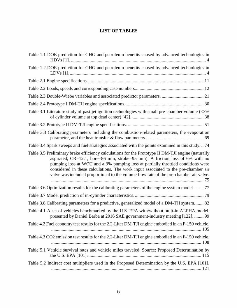
LIST OF TABLES

Table 1.1 DOE prediction for GHG and petroleum benefits caused by advanced technologies in

HDVs [1]. .................................................................................................................... 4

Table 1.2 DOE prediction for GHG and petroleum benefits caused by advanced technologies in

LDVs [1]. ..................................................................................................................... 4

Table 2.1 Engine specifications. ................................................................................................... 11

Table 2.2 Loads, speeds and corresponding case numbers. .......................................................... 12

Table 2.3 Double-Wiebe variables and associated predictor parameters. .................................... 21

Table 2.4 Prototype I DM-TJI engine specifications. ................................................................... 30

Table 3.1 Literature study of past jet ignition technologies with small pre-chamber volume (<3%

of cylinder volume at top dead center) [42]. .............................................................. 38

Table 3.2 Prototype II DM-TJI engine specifications. ................................................................. 51

Table 3.3 Calibrating parameters including the combustion-related parameters, the evaporation

parameter, and the heat transfer & flow parameters. ................................................. 69

Table 3.4 Spark sweeps and fuel strategies associated with the points examined in this study. .. 74

Table 3.5 Preliminary brake efficiency calculations for the Prototype II DM-TJI engine (naturally

aspirated, CR=12:1, bore=86 mm, stroke=95 mm). A friction loss of 6% with no

pumping loss at WOT and a 3% pumping loss at partially throttled conditions were

considered in these calculations. The work input associated to the pre-chamber air

valve was included proportional to the volume flow rate of the pre-chamber air valve.

................................................................................................................................... 75

Table 3.6 Optimization results for the calibrating parameters of the engine system model. ........ 77

Table 3.7 Model prediction of in-cylinder characteristics. ........................................................... 79

Table 3.8 Calibrating parameters for a predictive, generalized model of a DM-TJI system. ....... 82

Table 4.1 A set of vehicles benchmarked by the U.S. EPA with/without built-in ALPHA model,

presented by Daniel Barba at 2016 SAE government-industry meeting [122]. ........ 99

Table 4.2 Fuel economy test results for the 2.2-Liter DM-TJI engine embodied in an F-150 vehicle.

................................................................................................................................. 105

Table 4.3 CO2 emission test results for the 2.2-Liter DM-TJI engine embodied in an F-150 vehicle.

................................................................................................................................. 108

Table 5.1 Vehicle survival rates and vehicle miles traveled, Source: Proposed Determination by

the U.S. EPA [101]. ................................................................................................. 115

Table 5.2 Indirect cost multipliers used in the Proposed Determination by the U.S. EPA [101].

................................................................................................................................. 121

x

Table 5.3 Total fuel consumption and CO2 emission for the F-150 vehicle with the DM-TJI engine

compared to the same vehicle with its original engine, the 2.7-Liter EcoBoost®. The

effect of a 10-percent rebound effect is also shown in these calculations. .............. 123

Table 5.4 Costs and benefits associated with the Ford F-150 vehicle equipped with the DM-TJI

engine over the first three years of the vehicle’s life time, compared to the same vehicle

with its original engine, the 2.7-Liter EcoBoost®. The 10-percent rebound effect was

included in these calculations. ................................................................................. 126

Table 5.5 Costs and benefits associated with the Ford F-150 vehicle equipped with the DM-TJI

engine over the full life time of the vehicle, compared to the same vehicle with its

original engine, the 2.7-Liter EcoBoost®. The 10-percent rebound effect was included

in these calculations. ................................................................................................ 126

Table 5.6 Price equivalent of potential increase in benefits for a DM-TJI engine embodied in an

F-150 vehicle compared to the same vehicle with its base engine. An assumption was

made to increase the current fuel economy obtained for the DM-TJI engine with an

extra 5 and 10 percent. The CO2 emission was assumed to reduce with an extra 5 and

10 percent, accordingly. The 10-percent rebound effect is included in these

calculations. ............................................................................................................. 128

Table A.1 Energy requirements for the pre-chamber air valve. ................................................. 136

Table A.2 Fuel consumption calculations under highly dilute conditions.................................. 138

Table A.3 Combustion characteristics under highly dilute conditions. ...................................... 140

Table A.4 Friction calculations using Chen-Flynn Model. ......................................................... 142

xi

LIST OF FIGURES

Figure 1.1 Energy consumption by travel mode, quadrillion British thermal units. The chart is

directly taken from the EIA’s AEO 2018 [5]. ............................................................. 2

Figure 1.2 Transportation sector consumption by fuel type, quadrillion British thermal units. The

chart is directly taken from the EIA’s AEO 2018 [5]. ................................................. 3

Figure 1.3 Light-duty vehicle sales by fuel type, millions of vehicles. The chart is directly taken

from the EIA’s AEO 2018 [5]. .................................................................................... 3

Figure 2.1 In-cylinder rate of heat release for three loads of 60, 120, and 180 N-m at 2000 rpm.

The plots for 120 and 180 N-m were shifted to the left. ............................................ 23

Figure 2.2 Cumulative heat release results at 2000 rpm/120 N-m. .............................................. 23

Figure 2.3 Engine ignition delay – all cases studied. .................................................................... 24

Figure 2.4 Cylinder pressures, experiments vs. numerical predictions at 2000 rpm. ................... 25

Figure 2.5 Cylinder pressures, experiments versus numerical predictions – all cases studied; solid

and dash-dot lines represent the experiments and numerical prediction, respectively.

In subplots for speeds from 1500 rpm to 3000 rpm, traces with low, medium, and high

peak pressures represent loads of 60 N.m, 120 N.m, and 180 N.m; respectively. Traces

for 3500 rpm do not follow the general trend as others and the pressure traces for 180

N.m have peak pressures slightly lower than 120 N.m. Subplots for 4000 rpm and 4500

rpm represent loads of 60 N.m and 120 N.m with the low and high peak pressures,

respectively. ............................................................................................................... 26

Figure 2.6 Intercooler, intake manifold, coolant, and exhaust manifold temperature – all cases

studied. The load and speed associated to each of these case numbers can be found in

Table 2.2. ................................................................................................................... 27

Figure 2.7 In-cylinder temperature at spark timing for all the cases. The load and speed associated

to each of these case numbers can be found in Table 2.2. ......................................... 27

Figure 2.8 Double-Wiebe variables, direct calculations vs. linear model predictions; solid and

dashed lines represent the direct calculations and model predictions, respectively. The

load and speed associated with each of these case numbers can be found in Table 2.2.

................................................................................................................................... 28

Figure 2.9 Cumulative normalized apparent heat release, direct calculations vs. developed linear

model predictions at 2000 rpm. ................................................................................. 29

Figure 2.10 Cumulative normalized apparent heat release, direct calculations versus developed

linear model predictions – all cases studied; solid and dash-dot lines represent the

experiments and numerical predictions, respectively. In each subplot, the traces for the

cumulative heat release gradually shift to the right, as loads increase. ..................... 29

Figure 2.11 Normalized apparent heat release, homogeneous turbocharged GDI engine vs. DM-

TJI; speed of 1500 rpm and 𝐼𝑀𝐸𝑃𝑔 ~6 bar............................................................... 31

xii

Figure 2.12 Normalized in-cylinder heat transfer, homogeneous turbocharged GDI engine vs. DM-

TJI; speed of 1500 rpm and 𝐼𝑀𝐸𝑃𝑔 ~6 bar............................................................... 31

Figure 3.1 The drawing by Jean-Pierre Petit of a group of Cal bears forced to cultivate the field in

an overpopulated row [46]. ........................................................................................ 35

Figure 3.2 The drawing by Jean-Pierre Petit of a group of Cal bears cultivating the field in parallel

[46]. ............................................................................................................................ 35

Figure 3.3 Plot for conversion efficiency vs. air/fuel ratio (A/F) with typical air–fuel traces

(showing actual variations in air–fuel ratio under closed-loop control) from 1986 and

1990 cars; the figure is directly taken from the work by Gandhi et al. [96]. The

stoichiometric air/fuel ratio is about 14.7. ................................................................. 47

Figure 3.4 Design details for the pre-chamber of the Prototype II DM-TJI engine. .................... 49

Figure 3.5 Design details for the pre-chamber of the Prototype I DM-TJI engine. ...................... 49

Figure 3.6 Prototype II DM-TJI engine architecture. ................................................................... 50

Figure 3.7 Schematic of the dampener for the flow measurement of the pre-chamber purge valve

assembly. The inside and outside of the flexible membrane are filled by air at

approximately the same pressure. The flexible membrane absorbs the flow pulsations

upstream from the air valve, leading to a reliable flow measurement. ...................... 52

Figure 3.8 Prototype II DM-TJI engine at MSU EARL. .............................................................. 53

Figure 3.9 Modeling framework for system-level simulation of Prototype II DM-TJI engine. ... 56

Figure 3.10 Pre-chamber evaporation model developed for Prototype II DM-TJI engine. Step 1:

As the fuel injection happens, a portion of fuel will evaporate immediately at the time

of injection, “k” factor. The remaining (“1-k” factor), however, will form a thin fuel

film on the pre-chamber wall. Step 2: Combustion starts inside the pre-chamber

leading to the chemically active turbulent jets entering the main combustion chamber.

Step 3: Combustion starts inside the main chamber, leading to the flow being pushed

into the pre-chamber. The hot reacting pushed-back flow causes the pre-chamber fuel

film to evaporate. ....................................................................................................... 61

Figure 3.11 Mass transfer between pre- and main combustion chambers. Positive values present

the flow in the direction of pre- to the main chamber, while the negative values are for

the flow in the opposite direction (from main to the pre-chamber). The blue solid line

shows the crank-resolved model prediction of the mass flow rate. The green and

orange stars point to the start (𝜃𝑆𝑡𝑎𝑟𝑡) and end (𝜃𝐸𝑛𝑑) of the second fuel release into

the pre-chamber, respectively. ................................................................................... 62

Figure 3.12 Variable start of combustion (SOC) of parameter-varying Wiebe function. ............ 66

Figure 3.13 Parameter-varying Wiebe function vs. single-Wiebe function. The red circles display

the single-Wiebe function, while the green stars represent the parameter-varying

Wiebe function obtained using the variable SOC shown in Fig 3.12. The multi-color

solid lines are the single-Wiebe curves associated with the variable SOCs. ............. 66

Figure 3.14 Volume flow rate measured by the low range LFE at 1500 rpm with a WOT. ........ 72

xiii

Figure 3.15 Thermal efficiencies obtained for the Prototype II DM-TJI engine compared to an

engine run under SI-HCCI-SACI combustion strategies. The main figure is a

duplication of the results presented by Ortiz-Soto and colleagues in “Thermodynamic

efficiency assessment of gasoline spark ignition and compression ignition operating

strategies using a new multi-mode combustion model for engine system simulations”

[107]. The data from the Prototype II DM-TJI were added based on preliminary

efficiency calculations under lean operating conditions, lambda ~2. ........................ 76

Figure 3.16 Correlation plots for gross IMEP, main chamber peak pressure, and peak pressure

phasing of the main chamber. The high 𝑅2 values indicate the high level of correlation

between numerical predictions and experiments. ...................................................... 77

Figure 3.17 Model prediction vs. experiments for in-cylinder pressures of pre- and main

combustion chambers at 2000 rpm with a WOT. ...................................................... 78


combustion chambers at 2000 rpm with a throttle partially opened. ......................... 78


combustion chambers at 1500 rpm with a WOT. ...................................................... 78


combustion chambers at 1500 rpm with a throttle partially opened. ......................... 79

Figure 3.21 Modeling framework used in order to generate a full engine map, equivalent to the

power requirements of the Ford F-150 2.7-Liter EcoBoost®, for the DM-TJI engine

under highly dilute conditions. .................................................................................. 85

Figure 3.22 Brake thermal efficiency map of the DM-TJI engine in a four-cylinder boosted

configuration under highly dilute conditions up to 40% external EGR. ................... 87

Figure 3.23 Brake specific fuel consumption (BSFC in g/kW/hr) map of the DM-TJI engine in a

four-cylinder boosted configuration under highly dilute conditions up to 40% external

EGR. .......................................................................................................................... 87

Figure 3.24 Segmented warmed-up closed-throttle (CT) BMEP curve of the 2.7-Liter EcoBoost®

engine compared to the FMEP results obtained by the Chen-Flynn model at different

loads and speeds. ....................................................................................................... 89

Figure 3.25 Gross indicated efficiency with respect to BMEP. The dash-dot line displays the 23

bar BMEP. The loads beyond this point were obtained by reducing the charge dilution,

while the spark timings were retarded to maintain the 150 bar constraint for in-cylinder

pressures. ................................................................................................................... 90

Figure 3.26 Gross indicated efficiency with respect to CA50. The data report an average CA50 of

7.6 CADaTDCF as the optimum CA50 for the current simulations performed on the

DM-TJI engine. The data with retarded spark events were excluded in average value

calculation. ................................................................................................................. 90

Figure 3.27 Power requirements for delivering air to the pre-chamber of a DM-TJI engine as the

percentage of IMEPg. Details of these calculations were explained under “Energy

Input for a Pre-Chamber Air Valve” and summarized in Appendix A, Table A.1. .. 91

xiv



EGR. ........................................................................................................................ 103

Figure 4.2 Brake specific fuel consumption (BSFC in g/kW/hr) map of the 2.7-Liter EcoBoost®

embodied in an F-150 vehicle. ................................................................................. 104

Figure 4.3 The federal test procedure (FTP) which is composed of the urban dynamometer driving

schedule (UDDS), followed by the first 505 seconds of the UDDS [124]. ............. 105

Figure 4.4 The highway fuel economy test driving schedule (HWFET) which represents highway

driving conditions under 60 miles/hr [124]. ............................................................ 105

Figure 4.5 The US06 which is a high acceleration aggressive driving schedule and often called as

“supplemental FTP” driving schedule [124]. .......................................................... 106



EGR The green circles display the loads and speeds associated with the engine

performance over the EPA federal test procedure, the city cycle. ........................... 107



EGR. The green circles display the loads and speeds associated with the engine

performance over the EPA highway fuel economy test. ......................................... 107



EGR. The green circles display the loads and speeds associated with the engine

performance over the EPA high acceleration US06 driving schedule. ................... 108

Figure 5.1 Gasoline price projections for the years 2020 through 2050, Source: U.S. Energy

Information Administration. .................................................................................... 114

Figure 5.2 New SC-CO2 values reported by the Trump administration in a document titled

“Regulatory Impact Analysis for the Review of the Clean Power Plan: Proposal”

[135]. ........................................................................................................................ 119

Figure 5.3 New SC-CO2 values at 3% discount rate compared to the former prices for the SC-CO2

reported by the IWG at the same discount rate. The new SC-CO2 values demonstrate

an average of 86% reduction compared to the former values. ................................ 119

Figure 5.4 Price equivalent of total fuel consumed, and CO2 produced for the DM-TJI engine

compared to the 2.7-Liter EcoBoost®. The effect of a 10-percent rebound effect is also

depicted. ................................................................................................................... 124

Figure 5.5 Benefits obtained by the DM-TJI engine compared to the 2.7-Liter EcoBoost®. The

10-percent rebound effect was included in these calculations. ................................ 124

Figure 5.6 Price estimates of CO2 emission for a DM-TJI engine over the life time of the vehicle

in which embodied. The new SC-CO2 at 3% discount rate was increased incrementally

to match the former SC-CO2 reported by the IWG at the same discount rate. The 10-

percent rebound effect was included in these calculations. ..................................... 125

xv

Figure 5.7 Potential improvements in benefits of a DM-TJI engine compared to the base engine if

the current fuel economy obtained for the DM-TJI engine were to increase by an extra

5 and 10 percent. The 10-percent rebound effect is included in these calculations. 128

1

CHAPTER 1

INTRODUCTION

1.1 Background and Motivation

Transportation consumes 70% of all U.S. petroleum use annually, contributing 1.8 gigatons of

carbon dioxide (CO2)-equivalent greenhouse gas (GHG) emissions [1]. Transportation is the

United States’ second biggest source of CO2 emission, with 27% of U.S. totals [1,2]. Worldwide

energy demands for transportation are predicted to rise substantially as the economy grows and

the growing middle class aims to access more transportation [3]. The question then arises: what is

the mobility for the future? Over the past decade or so, there has been a dramatic focus on electric

vehicles (EVs) as a solution toward energy demands in the mobility system. However, are EVs

going to take over internal combustion (IC) engines and if so, how fast will that happen? John

Heywood briefly responds to this question in MIT News on April 18, 2018. He says [4]: “Electric

vehicles are certainly going to play a useful role moving forward, but right now it is really difficult

to estimate how big a role they will eventually play.”

Transportation is a complex system consisting of all different modes of travel. It includes inland

surface transport, sea transport, air transport, and transport through pipelines. Among all, the

combination of light-duty vehicles, medium-duty/heavy-duty trucks, and commercial light trucks

accounts for 78% of the total energy consumed in the transportation sector in year 2010. This

consumption is projected to mildly decrease to 70% by the year 2050 [5]. Figure 0.1 represents the

2

energy consumption by travel mode in quadrillion British thermal units for the years 2010 through

2050.

Additionally, the consumption of motor gasoline and distillate fuel oils (which includes diesel fuels

and fuel oils) combined accounts for 82% of total energy consumed in the transportation sector in

the year 2010, with a projection of 70% in the year 2050 as the use of alternative fuels increases

[5]. Figure 0.2 displays the transportation sector consumption by fuel type in quadrillion British

thermal units for the range of years reported by the Energy Information Administration (EIA) in

their Annual Energy Outlook (AEO) 2018 [5].

Figure 0.1 Energy consumption by travel mode, quadrillion British thermal units. The chart is directly taken from the EIA’s AEO

2018 [5].

Figure 0.3 shows light-duty vehicle sales by fuel type, millions of vehicles, for the years 2010 to

2050 (projected value). As one can see, although the combined share of sales attributable to

gasoline and flex-fuel vehicles declines (from 95% in 2017 to 78% in 2050), gasoline vehicles

remain the dominant vehicle type through 2050 based on current predictions [5]. Flex-fuel vehicles

use gasoline blended with up to 85% ethanol.

0

5

10

15

20

25

30

2010 2020 2030 2040 2050

QU

AD

RIL

LIO

N B

RIT

ISH

TH

ERM

AL

UN

ITS

YEAR

light-dutyvehiclesmedium and heavy dutyaircommerciallight trucksrailmarineother

2017

HISTORY PROJECTIONS

3

Figure 0.2 Transportation sector consumption by fuel type, quadrillion British thermal units. The chart is directly taken from the

EIA’s AEO 2018 [5].

Figure 0.3 Light-duty vehicle sales by fuel type, millions of vehicles. The chart is directly taken from the EIA’s AEO 2018 [5].

As statistics demonstrate, the number of vehicles powered by a source of energy other than

traditional petroleum fuels, including electric vehicles, will increase as time passes. However, it

seems that vehicles run on liquid fuels will be the major source of transportation for years to come.

Thus, improving fuel economy of gasoline and diesel vehicles plays an important role toward

0

5

10

15

20

25

30

2010 2020 2030 2040 2050

QU

AD

RIL

LIO

N B

RIT

ISH

TH

ERM

AL

UN

ITS

YEAR

motorgasoline

distillatefuel oil

jet fuelelectricityother

0

2

4

6

8

10

12

14

16

18

20

2010 2020 2030 2040 2050

MIL

LIO

NS

OF

VEH

ICLE

S

YEAR

otherhybrid electricplug-in hybrid electricbattery electricdieselflex fuelgasoline

2017

HISTORY PROJECTIONS

2017

HISTORY PROJECTIONS

4

reducing the environmental impacts on air quality and health, GHG emissions, and national oil

dependency; all of which are caused as negative side effects of transportation powered by

petroleum-derived fuels.

The Department of Energy (DOE) reports several approaches and technology improvement in their

quadrennial technology review of 2015 for light duty (LD) and heavy-duty vehicles (HDVs) [1].

Tables 0.1 and 0.2 present the predicted gains in both GHG and petroleum reduction for different

approaches studied.

Table 0.1 DOE prediction for GHG and petroleum benefits caused by advanced technologies in HDVs [1].

HDV GHG Benefit Petroleum Benefit Timing

Combustion 25% 25% Near

Systems 20% 20% Near

Table 0.2 DOE prediction for GHG and petroleum benefits caused by advanced technologies in LDVs [1].

LDV GHG Benefit Petroleum Benefit Timing

Combustion 25% 25% Near

Systems 20% 20% Near

Advanced Materials 20% 20% Mid

Electrification 80% 80% Mid

Fuel Cell 80% 80% Long

As one can see, combustion improvement has been listed as one of the two near-term advances in

technology toward reduction of both GHG and petroleum consumption. Advanced combustion

strategies can be obtained through highly dilute and low-temperature combustion (LTC) modes in

internal combustion (IC) engines. The Dual Mode, Turbulent Jet Ignition (DM-TJI) system is a

distributed combustion technology to achieve LTC modes in spark ignition (SI) engines. The DM-

TJI engine demonstrated the potential to provide diesel-like efficiencies and engine-out emission

which can be controlled using a three-way catalytic converter.

Currently, there is not a model capable of estimating the fuel consumption and emission for a DM-

TJI engine over standardized city/highway driving cycles. A driving cycle is a fixed schedule of a

5

vehicle operation, defined in legislation, to test the real-world operation of the vehicle. In this

dissertation, the path from engine experiments toward model development of a DM-TJI engine is

described. The focus of this study is to project the fuel consumption and CO2 emission for a vehicle

equipped with the DM-TJI combustion technology over real-world driving cycles.

1.2 Structure of Dissertation

The dissertation is organized as follows. Chapter 2 describes a study done on a set of data collected

from a 2013 Ford Escape 1.6-Liter EcoBoost® turbocharged gasoline direct injection (GDI)

engine, tested at the U.S. Environmental Protection Agency (EPA). A zero-dimensional (0D)

combustion model was developed and validated for the GDI engine operated at a wide range of

loads and speeds. This study is believed to act as a foundation for future work to compare the

combustion behavior of a production-based GDI engine with that of a DM-TJI engine.

Chapter 3 includes experiments and model development of a DM-TJI engine. Engine experiments

were conducted on a single-cylinder DM-TJI engine at Michigan State University. A zero-

dimensional/one-dimensional (0D/1D) engine simulation was performed using GT-SUITE/GT-

POWER and the model developed was calibrated based on experimental data. The calibrated

engine system model was further studied to propose a predictive, generalized model for a DM-TJI

engine. An engine fuel map was, then, generated using the generalized model for the DM-TJI

engine covering a wide range of loads and speeds.

In Chapter 4, the engine fuel map, generated by the predictive, generalized model in Chapter 3,

was translated into vehicle fuel consumption and CO2 emission over light-duty vehicle driving

cycles. The drive cycle analysis was conducted using the U.S. EPA advanced light-duty powertrain

and hybrid analysis (ALPHA) vehicle simulator tool.

6

Chapter 5 describes a cost-benefit analysis which was performed based on the results obtained

from vehicle simulation using the EPA ALPHA model. This chapter is concluded with the

comparison between the results of the cost-benefit analysis for a vehicle equipped with the DM-

TJI system and those of the same vehicle with a production-based GDI engine.

The dissertation ends with concluding remarks and recommended steps for future work in Chapter

6.

1.3 Specific Aims

The specific aims for each of the chapters in this dissertation are summarized below.

Chapter 1:

• Briefly discuss the ongoing needs to improve brake efficiency of internal combustion (IC)

engines.

Chapter 2:

• Develop a zero-dimensional (0D) combustion model for a gasoline direct injection (GDI)

engine.

• Set the ground for future work where the combustion behavior of a production-based GDI

engine would be compared to that of a Dual Mode, Turbulent Jet Ignition (DM-TJI) engine.

Chapter 3:

• Numerically predict the ancillary work requirement to operate the DM-TJI system.

• Map the path from engine experiments toward model development of a DM-TJI engine

with a pre-chamber air valve assembly.

7

• Propose a predictive, generalized model for a DM-TJI engine, with minimal experimental

input.

• Generate a complete fuel map for the DM-TJI engine in a boosted highly-dilute

configuration

Chapter 4:

• Demonstrate a general understanding of the U.S. EPA ALPHA model.

• Predict fuel economy and CO2 emission for a vehicle equipped with the DM-TJI

combustion technology and compare the results obtained with those of the same vehicle

with its original engine.

Chapter 5:

• Map the path to conduct a cost-benefit analysis following the methodology taught by the

U.S. EPA in their “Proposed Determination on the Appropriateness of the Model Year

2022-2025 Light-Duty Vehicle Greenhouse Gas Emissions Standards under the Midterm

Evaluation: Technical Support Document.”

• Perform the cost-benefit analysis of a vehicle equipped with the DM-TJI combustion

technology and compare the results obtained to those of the same vehicle with its original

engine.

Chapter 6:

• Conclude and recommend the steps for future work.

8

CHAPTER 2

COMBUSTION MODEL FOR A HOMOGENEOUS

TURBOCHARGED GASOLINE DIRECT INJECTION ENGINE

2.1 Introduction

In recent years, a range of different technologies has been under consideration to improve the fuel

economy of gasoline engines and reduce exhaust emissions. Among these, gasoline direct injection

(GDI) engines have shown significant market acceptance [6,7]. Therefore, a large portion of light-

duty vehicle developments leans toward achieving higher thermal efficiency and lower exhaust

emissions using GDI engines. Recent GDI engines include substantial technology developments

[8] such as:

• Higher compression ratio

• Charge dilution using exhaust gas recirculation (EGR)

• Tumble enhancement

• Higher ignition energy

• Late intake valve closure timing (Miller cycle)

Direct injection of the fuel into the combustion chamber decreases the charge temperature,

resulting in higher volumetric efficiency and less knock tendency at higher compression ratios.

These characteristics lead to higher thermal efficiency and power output for GDI engines which

facilitate engine downsizing. GDI engines can be designed to operate in both homogeneous and

lean stratified modes of operation. Homogeneous charge is obtained through early intake injection

9

of the fuel. Stratified charge, on the other hand, is attained as a result of a late fuel injection during

compression stroke. This causes a local fuel-rich mixture in the vicinity of the spark plug,

surrounded by a globally fuel-lean mixture in the combustion chamber. At engine low-to mid-load

operation, the homogeneous mode with its higher combustion stability lacks the advantage of

lower pumping work compared to the lean stratified mode. Combustion stability is challenging to

obtain in lean stratified mode due to high cycle-to-cycle variability of in-cylinder charge motion

and quenching of the flame. Today, however, the majority of engines operate in homogeneous

mode of operation.

2.2 Objective

The importance of GDI engines in current and future markets is identified, and it is worthwhile to

develop predictive combustion models that allow the engine developers to find optimal operating

conditions. There have been several published numerical and experimental investigations on GDI

engines. Fuel economy and exhaust emissions were numerically and/or experimentally studied

under different injection strategies and advanced injection systems [9–12]. Berni et al. examined

the effects of water/methanol injection as knock suppressor on a downsized GDI engine [13].

Simulations of in-cylinder charge motion, spray development, and wall impingement in GDI

engines were performed by Lucchini et al. and Fatouraie et al. [14,15]. Cho et al. investigated the

combustion and heat transfer behavior in a single-cylinder GDI engine [16]. The aforementioned

studies cover a wide variety of subjects. However, the current author did not find any in-depth

investigation on the zero-dimensional combustion model of a GDI engine.

Burnt et al. and Egnell conducted a single-zone heat release analysis on direct-injection diesel

engines [17,18]. Dowell and colleagues meticulously evaluated the heat release modeling of

10

modern high-speed diesel engines [19]. Lindström et al. reported an empirical combustion model

for a port fuel injection (PFI) spark ignition engine [20]. Hellström et al. and Prakash et al. [21,22]

have done studies on the combustion model of spark-assisted compression ignition (SACI)

engines. Spicher et al. showed GDI development potentialities and compared the heat release

behavior of PFI and GDI engines [23]. Huegel et al. investigated the heat transfer of a single-

cylinder GDI engine with a side study on the heat release behavior of the engine in both

homogeneous and stratified modes of operation [24]. Results obtained in the current study well

agree with the works done by Spicher and Huegel describing heat release behavior and

consequently the combustion model of a GDI engine.

The primary goal of this chapter is to develop a zero-dimensional (0D) combustion model which

can be used towards the whole-cycle simulation of a GDI engine. However, the study covers a

preliminary heat release analysis of a Dual Mode, Turbulent Jet Ignition (DM-TJI) engine and

compares the results obtained with those of the GDI engine. The results for the heat release analysis

of the DM-TJI engine in comparison with the GDI engine are presented in a short section at the

end of this chapter, Section 2.6.

This chapter is organized as follows. The experimental arrangement is first described. After that

the numerical approach and model development are explained, followed by the section providing

the numerical results using experimental data and the discussion of the results. A short section, at

the end of this chapter, covers the preliminary results for the heat release behavior of a DM-TJI

engine and compares the combustion characteristics of current homogeneous turbocharged GDI

engine with those of the DM-TJI engine. Conclusions are drawn in the last section.

11

2.3 Experimental Arrangement

2.3.1 Experimental Setup

Experimental data was collected from a 2013 Ford Escape 1.6-Liter EcoBoost® turbocharged GDI

engine. To make use of the stock engine and vehicle controllers, the engine was tethered to its

vehicle located outside the test cell. Details of the test site, vehicle tether information, engine setup,

engine systems including intake/exhaust, charge air cooling, cooling system, oil system, and front

end accessory drive (FEAD) can be found in the work done by Stuhldreher and colleagues [25].

Engine specifications are listed in Table 2.1.

Table 2.1 Engine specifications.

Vehicle (MY, Make, Model) 2013 Ford Escape

Engine (Displacement, Name) 1.6 L EcoBoost®

Rated Torque 240 N-m @ 1600-5000 RPM

Rated Power 180 hp @ 5700 RPM

Compression Ratio 10:1

No. of Cylinders 4

Firing Order 1-3-4-2

Fuel Injection Common rail

Fuel Type LEV III regular gasoline

2.3.2 Data Set Definition

The data logged included engine torque, fuel flow rate, air flow rate, pressures, temperatures, in-

cylinder pressure, and OBD/extended proportional-integral-derivative (PID) controller area

network (CAN) data.

2.3.3 Data Collection Procedure

Two data acquisition systems were used. The first was an A&D Technology iTest Test System

Automation Platform for low-frequency data at a rate of 10 Hz. The second was an A&D

Technology Combustion Analysis System (CAS) for high-frequency data acquisition. CAS was

sampled at 0.1 crank angle resolution and calculated results were transmitted to iTest at 10 Hz rate.

12

The engine with its associated engine control unit (ECU) operates under original equipment

manufacturer (OEM) specific protection modes. These protection modes limit the engine operation

in a test cell, especially at higher loads as engine temperatures reach the safety thresholds. To

obtain experimental data, two test procedures were used to compensate for the protection modes.

The first procedure was used for the loads below ~70% of the maximum rated torques at which

the engine temperatures remain within the safety thresholds. During this procedure, a set of

selected parameters was used as stability criteria. These parameters included fuel flow, torque, and

turbine inlet temperature. The settling time ranged from 20 seconds to 30 seconds at different loads

and speeds.

The second procedure was used to obtain high-load data which go beyond OEM safety thresholds.

It should be noted that in real-world driving the engine does not remain at high-load operating

conditions for more than a few seconds. Thus, the quasi-steady-state values were of interest for

the high-load operating points beyond the OEM safety thresholds. This second procedure started

with the engine being set to the desired speed and a load of 10 N-m. The data logger was triggered

on and the load stepped to the desired value. The data was logged for 20 seconds in total before

the engine was brought back to the cool-down mode of 1500 rpm and 10 N-m.

Table 2.2 Loads, speeds and corresponding case numbers.

Load (N-m)

60 120 180

Sp

eed

(R

PM

)

1500 1 2 3

2000 4 5 6

2500 7 8 9

3000 10 11 12

3500 13 14 15

4000 16 17 −

4500 18 19 −

13

Details of these test procedures can be found in the study by Stuhldreher et al. [25]. A total of 50

cycles was used for the current study at each operating condition. Table 2.2 shows all the cases

studied here. It should be noted that the engine was always operated at stoichiometric condition.

2.4 Numerical Approach and Model Development

The current study performed a zero-dimensional/one-dimensional (0D/1D) simulation with a

single-zone thermodynamic analysis of the cylinder. Engine modeling can be broadly separated

into two different categories, 0D/1D engine simulation tools and high-fidelity three-dimensional

(3D) modeling platforms. The 0D/1D simulation tools are used for engine studies and

optimizations, when computationally expensive 3D simulations are impractical. More information

on different approaches in engine modeling can be found in Section 3.5, under “Modeling

Platform” (3.5.1).

2.4.1 Heat Release Analysis

The single-zone analysis applied in the current work considered the change in sensible internal

energy (first term on the right-hand side of Equation 2.1 ), work done by the piston motion (second

term); and heat transfer from in-cylinder gas to the walls (𝑄ℎ.𝑡). The effects of blow-by and

crevices were assumed to be negligible. The energy equation is written as [26,27]:

𝑑𝑄𝑐ℎ

𝑑𝑡=

1

𝛾 − 1 𝑉

𝑑𝑝

𝑑𝑡+

𝛾

𝛾 − 1 𝑝

𝑑𝑉

𝑑𝑡+

𝑑𝑄ℎ.𝑡

𝑑𝑡 (2.1)

where, 𝑄𝑐ℎ is the apparent total heat release in kJ; 𝛾 is the specific heat ratio; 𝑉 is the in-cylinder

volume in m3; 𝑝 is the in-cylinder pressure in kPa; and 𝑄ℎ.𝑡 is the heat transfer to the walls in kJ.

14

2.4.1.1 Net Heat Release

The summation of change in sensible internal energy and work done by the piston is commonly

called net heat release. When the in-cylinder pressure and volume are known, net heat release can

be calculated if the dependency of specific heat ratio, or gamma, on temperature is well defined.

In general, gamma is a function of both temperature and mixture composition. However, as Chang

et al. showed [28], ignoring the gamma dependency on mixture composition leads to a negligible

error. They reported a third-order polynomial gamma dependency on temperature as a result of

curve-fitting at a median air/fuel ratio. This polynomial (Equation 2.2) was used in the current

work.

𝛾 = −9.97 × 10−12𝑇3 + 6.21 × 10−8𝑇2 − 1.44 × 10−4𝑇 + 1.40 (2.2)

where, 𝛾 and 𝑇 are specific heat ratio and temperature, respectively.

Average in-cylinder temperature was determined from the ideal gas law using the total mass

trapped in the cylinder at the intake/exhaust valve closing (IVC/EVC), the in-cylinder pressure at

each crank angle, and the corresponding in-cylinder volume. This temperature was believed to be

close to the mass-averaged cylinder temperature during combustion, since the molecular weights

of burned and unburned mixtures are basically the same [26]. Trapped in-cylinder mass can be

calculated as a summation of trapped air, fuel, internal exhaust gas recirculation (EGR), and

external EGR in the combustion chamber. There was no external EGR for any of the cases under

study. Thus, the term was set to zero.

The internal EGR was calculated using the Yun and Mirsky correlation [29]. An iterative algorithm

was used to find gamma and in-cylinder temperature at IVC. The in-cylinder temperature at IVC

can be calculated as a weighted average of intake temperature and exhaust temperature at intake

pressure as follows [20].

15

𝑇𝑒𝑥ℎ∗ = 𝑇𝑒𝑥ℎ (

𝑝𝑖𝑛𝑡

𝑝𝑒𝑥ℎ)

(𝛾−1)/𝛾

(2.3)

𝑥𝑟 =𝑉𝐸𝑉𝐶

𝑉𝐸𝑉𝑂(

𝑃𝐸𝑉𝐶

𝑃𝐸𝑉𝑂)

1/𝛾

(2.4)

𝑇 = (1 − 𝑥𝑟)𝑇𝑖𝑛𝑡 + 𝑥𝑟𝑇𝑒𝑥ℎ∗ (2.5)

where, 𝑇𝑒𝑥ℎ∗ is the exhaust temperature at intake pressure; 𝑇𝑒𝑥ℎ is the exhaust temperature; 𝑝𝑒𝑥ℎ is

the exhaust pressure; 𝑉 is the in-cylinder volume; and 𝑥𝑟 is the internal residual gas fraction. In

addition, subscripts 𝑖𝑛𝑡, 𝐸𝑉𝐶, and 𝐸𝑉𝑂 denote intake, exhaust valve closing, and exhaust valve

opening; respectively.

2.4.1.2 Heat Transfer Model

The GT-POWER WoschniGT heat transfer model was used to simulate the heat transfer term in

the energy equation of the heat release analysis. WoschniGT closely matches the classical Woschni

correlation without swirl. The most important difference lies in the treatment of heat transfer

coefficients when the intake and exhaust valves are open, and intake inflow velocities and exhaust

backflow velocities increase the in-cylinder heat transfer. The heat transfer coefficient in the

WoschniGT correlation is calculated as follows.

ℎ𝑐 𝑊𝑜𝑠𝑐ℎ𝑛𝑖 =𝐾1𝑝0.8𝑤0.8

𝐵0.2𝑇𝐾2 (2.6)

where, ℎ𝑐 𝑊𝑜𝑠𝑐ℎ𝑛𝑖 is the convective heat transfer coefficient in Wm2K⁄ ; 𝑝 is the in-cylinder

pressure in kPa; 𝑤 is the average cylinder gas velocity in m/s; 𝐵 is the cylinder bore in m; and 𝑇

is the in-cylinder temperature in K. Additionally, k1 and 𝑘2 are given constants as 3.01 and 0.50,

respectively. The average cylinder gas velocity is calculated in Equation. 2.7.

𝑤 = 𝐶1�̅�𝑝 +𝐶2(𝑉𝑑𝑇𝑟)

𝑃𝑟𝑉𝑟

(𝑝 − 𝑝𝑚) (2.7)

16

where, 𝑆�̅� is the mean piston speed in m/s; 𝑉𝑑 is the displacement volume in m3; 𝑇𝑟 is the working

fluid temperature prior to combustion in K; 𝑃𝑟 is the working fluid pressure prior to combustion in

kPa; 𝑉𝑟 is the working fluid volume prior to combustion in m3; 𝑝 is the in-cylinder pressure in kPa;

and 𝑝𝑚 is the motoring in-cylinder pressure at the same angle as p in kPa.

The 𝑐1 and 𝑐2 are constants calculated as below, Equations 2.8 and 2.9.

C1 = 2.28+3.90 min (Net mass flow into cylinder from valves

Trapped Mass∗Engine Frequency, 1)

(2.8)

C2 = {0 During cylinder gas exchange and compression3.24E − 3 During combustion and expansion

(2.9)

After calculation of the heat transfer coefficient using WoschniGT formulation (Equations 2.6,

2.7, 2.8, 2.9), the rate of in-cylinder heat transfer can be calculated as below, Equation 2.10. Since

there was no temperature data available for the piston, head, and liner of this Ford EcoBoost®

engine, the temperature profiles were extracted from the work by Huegel et al. on a single-cylinder

GDI engine [24]. A heat transfer multiplier (HTM) was used to adjust the heat transfer term,

assuming the combustion efficiency as 99.9% with no blow-by or crevice losses.

𝑑𝑄ℎ.𝑡

𝑑𝑡= 𝐻𝑇𝑀 ℎ𝑐 (

𝐴𝑝𝑖𝑠𝑡𝑜𝑛(𝑇 − 𝑇𝑤𝑎𝑙𝑙, 𝑝𝑖𝑠𝑡𝑜𝑛) +

𝐴ℎ𝑒𝑎𝑑(𝑇 − 𝑇𝑤𝑎𝑙𝑙, ℎ𝑒𝑎𝑑) +

𝐴𝑙𝑖𝑛𝑒𝑟(𝑇 − 𝑇𝑤𝑎𝑙𝑙, 𝑙𝑖𝑛𝑒𝑟)

) (2.10)

where, 𝑄ℎ.𝑡, 𝐻𝑇𝑀, ℎ𝑐, 𝐴, and 𝑇 represent the in-cylinder rate of heat transfer, the heat transfer

multiplier, the heat transfer coefficient, the surface area, and the in-cylinder temperature;

respectively.

17

2.4.1.3 Start of Combustion

Several approaches can be found in the literature to define start of combustion (SOC). Reddy et

al. studied determination of SOC based on first and second derivative of in-cylinder pressure [30].

Hariyanto et al. applied the wavelet analysis to define SOC of a diesel engine [31]. Shen et al. and

Bitar et al. defined SOC as the start for the dynamic stage of combustion, which corresponds to

the transition between compression and expansion processes; using a pressure-volume (P-V)

diagram [32,33]. Katrašnik et al. developed a new criterion to determine SOC [34]. Their study

mathematically demonstrated the delay in SOC prediction using the first and second derivatives

of in-cylinder pressure. They proposed a SOC criterion based on the local maximum of third

derivative of in-cylinder pressure with respect to crank angle. Determination of SOC using wavelet

analysis requires the engine vibration data which was not available. Additionally, Hariyanto et al.

showed a high degree of correlation between the results from their wavelet analysis and the SOC

criterion of the Katrašnik group. The accuracy of SOC determination methods based on the P-V

diagram depends on a level of judgment in defining SOC as the point in which the straight portion

of compression stroke deviates from its averaged path.

The current work used the SOC criterion by Katrašnik group. Signal preparation for in-cylinder

pressures was done using a MATLAB filtering algorithm called “filtfilt.” This algorithm performs

a zero-phase forward and reverse filtration. Design specifications were set to a third-order

Butterworth filter with a 0.1 normalized cutoff frequency for the 3 dB point, corresponding to 450

Hz – 1350 Hz for different speeds. The ignition delay was defined as the difference between spark

timing and calculated SOC for the range of speeds and loads studied.

18

2.4.2 Combustion Model

Ivan Wiebe was one of the pioneers to connect the rate of combustion to chain chemical reactions

in an internal combustion engine [21,35]. In real combustion systems, chain reactions progress

sequentially and in parallel with reactions involved in the formation of intermediate species called

“active centres” [35]. Active centres, which were referred to as effective centres by Wiebe, initiate

effective reactions which result in the formation of combustion products. The well-known Wiebe

function was developed on the basis of this concept [35].

The current work demonstrates a two-stage heat release phenomenon for the studied GDI engine.

Thus, a single Wiebe function is not suitable to capture the heat release characteristics of the engine

wherein pre-mixed combustion is followed by a diffusion-like combustion. “Diffusion-like”

combustion here is characterized with the slow-rate combustion as a result of either mixture

inhomogeneity or wall impingement. The mixture inhomogeneity can arise due to locally fuel-rich

regions, thereby leading to a slow-rate combustion. The wall impingement, on the other hand, can

result from fuel film deposition or flame hitting the wall. The deposited fuel film can evaporate in

the course of combustion, resulting in the second stage of heat release. Also, the heat losses when

the flame reaches the chamber walls would slow down the rate of combustion.

The current study used a double-Wiebe function to fit the results of heat release calculation; see

Equation 2.11.

𝑥𝑏(𝜃) = 𝑎𝑙𝑝ℎ𝑎 {1 − 𝑒𝑥𝑝 [−𝑎 (𝜃 − 𝜃0

∆𝜃1)

𝑚1+1

]} +

(1 − 𝑎𝑙𝑝ℎ𝑎) {1 − 𝑒𝑥𝑝 [−𝑎 (𝜃 − 𝜃0

∆𝜃2)

𝑚2+1

]}

(2.11)

19

where, a = −ln0.001 = 6.9, and 𝛼 is the switch point from the 1st Wiebe function to the 2nd; 𝜃 is

the instantaneous crank angle degree; 𝜃0 is the start of combustion; ∆𝜃1 and ∆𝜃2 are the total burn

durations for the 1st and 2nd Wiebe functions; and 𝑚1 and 𝑚2 are the combustion mode parameters

or Wiebe exponents for the 1st and 2nd Wiebe functions.

2.4.2.1 Semi-Predictive Combustion Model

The double-Wiebe function includes six unknown variables, 𝛼, 𝑚1, 𝑚2, ∆𝜃1, and ∆𝜃2, and the

SOC (𝜃0). The first five variables were determined based on a non-linear least-squares

optimization using MATLAB Curve Fitting Toolbox™. The SOC was determined using the

Katrašnik et al. criterion as mentioned earlier. A total of six look-up tables, one for each variable,

was built for different loads and speeds. These look-up tables were used in the GT-POWER model

as discussed next.

2.4.2.2 GT-POWER Model

The effectiveness of the semi-predictive combustion model was tested by comparing the

experimental in-cylinder pressures with results obtained from a model built using the 0D/1D

engine simulation tool, GT-SUITE/GT-POWER (Gamma Technologies). The six variables of the

double-Wiebe function, used to model the two-stage combustion behavior of the GDI engine, were

defined in GT-POWER by importing the look-up tables built from the semi-predictive combustion

model. The GT-POWER model simulates the engine components from intercooler outlet to turbine

inlet. Component characteristics were set based on experimentally measured data and 3D

computer-aided design (CAD) models including: valve geometries, timings, lift profiles, and

discharge coefficients; in-cylinder and port geometries; injection timings and durations, and

air/fuel ratio. The engine induction and exhaust system were built to a close approximation, as

there was no CAD model available. The intake manifold throttle angle was controlled using a

http://gasturbinespower.asmedigitalcollection.asme.org/solr/searchresults.aspx?author=Toma%c5%be+Katra%c5%a1nik&q=Toma%c5%be+Katra%c5%a1nik

20

proportional-integral (PI) controller with brake mean effective pressure (BMEP) as its input value.

The in-cylinder heat transfer model was set to WoschniGT with the same in-cylinder temperatures

and heat transfer multiplier of heat release analysis described earlier. The combustion model was

imposed based on results obtained from the semi-predictive combustion model.

2.4.2.3 Predictive Combustion Model

The semi-predictive combustion model, verified using the GT-POWER simulation, was further

studied to find correlations for each of the six variables of the double-Wiebe function. The

corresponding combustion model, called “predictive combustion model,” can correlate the

combustion behavior of the GDI engine to a set of engine parameters. The predictor parameters

(𝑥1 to 𝑥4) chosen for each of these variables are listed in Table 2.3. The linear correlations, as

shown in Expression 2.12, were found to well predict the six variables. The first four variables:

𝜃0, 𝛼, ∆𝜃1, and ∆𝜃2; were predicted using the manifold temperature (𝑇𝑚𝑎𝑛), internal EGR (𝑖𝐸𝐺𝑅),

engine speed, and ignition timing (𝜃𝑖𝑔𝑛). However, the behavior of last two variables, 𝑚1 and 𝑚2,

were best captured by using ∆𝜃1 and ∆𝜃2, respectively, along with 𝑖𝐸𝐺𝑅 and 𝑆𝑝𝑒𝑒𝑑 as model

predictor parameters (see Table 2.3). Thus, the same linear correlation shown in Expression 2.12

was used for 𝑚1 and 𝑚2, excluding the 𝑥4 parameter. A variety of parameters were examined to

define these dependencies. It seems that the engine in-cylinder characteristics at different loads

and speeds could be well captured by current predictor parameters. The combination of manifold

temperature and fraction of internal EGR was believed to act as an indicator of the boundary

temperature. The speed parameter could play a role in capturing the in-cylinder turbulence. The

ignition timing, along with three other parameters, could represent the effect of flame initiation on

the combustion behavior.

21

𝑎0 + 𝑎1𝑥1 + 𝑎2𝑥2 + 𝑎3𝑥3 + 𝑎4𝑥4 (2.12)

where, 𝑎0 to 𝑎4 are constants calculated from the results obtained for the semi-predictive

combustion model using linear regressions.

Table 2.3 Double-Wiebe variables and associated predictor parameters.

Variables 𝒙𝟏 𝒙𝟐 𝒙𝟑 𝒙𝟒

𝜽𝟎 𝑇𝑀𝑎𝑛 𝑖𝐸𝐺𝑅 𝑆𝑝𝑒𝑒𝑑 𝜃𝑖𝑔𝑛

𝜶 𝑇𝑀𝑎𝑛 𝑖𝐸𝐺𝑅 𝑆𝑝𝑒𝑒𝑑 𝜃𝑖𝑔𝑛

∆𝜽𝟏 𝑇𝑀𝑎𝑛 𝑖𝐸𝐺𝑅 𝑆𝑝𝑒𝑒𝑑 𝜃𝑖𝑔𝑛

∆𝜽𝟐 𝑇𝑀𝑎𝑛 𝑖𝐸𝐺𝑅 𝑆𝑝𝑒𝑒𝑑 𝜃𝑖𝑔𝑛

𝒎𝟏 ∆𝜃1 𝑖𝐸𝐺𝑅 𝑆𝑝𝑒𝑒𝑑 −

𝒎𝟐 ∆𝜃2 𝑖𝐸𝐺𝑅 𝑆𝑝𝑒𝑒𝑑 −

A least-squares optimization was performed using the MATLAB algorithm “LinearModel.fit” to

minimize the root-mean-square (RMS) error in the prediction of each variable. The linear

correlations found here were validated by regenerating the experimental cumulative heat release

as discussed later.

2.5 Results and Discussion

The following discussion for the GDI engine is divided into three parts. The first part covers the

results obtained for the heat release analysis including the ignition delays at different loads and

speeds. The second part discusses the results for the semi-predictive combustion model. These

results are followed by a comparison between the experimental and model regeneration of engine

heat release in the third part.

2.5.1 Heat Release Analysis

The results obtained from the heat release analysis demonstrated rapid initial pre-mixed

combustion (stage 1) followed by a gradual diffusion-like state of combustion (stage 2) for all the

loads and speeds studied in this homogeneous charge GDI engine. Figure 2.1 shows the heat

22

release rate for the loads of 60, 120, and 180 N-m at 2000 rpm. Pre-mixed and diffusion-like phases

of combustion are clearly noticeable in this figure. To highlight the two stages of combustion in

the figure, the rates of combustion at 120 and 180 N-m were shifted to the left with an offset of 6

and 19 crank angle degrees, respectively, to match their SOCs with that of the 60 N-m load. The

end point for the pre-mixed combustion is the start point of the diffusion-like phase of combustion

which continues up to nearly exhaust valve opening (EVO). The switch point from pre-mixed to

diffusion-like phases of combustion was determined as the point where the double-Wiebe function

shifts from the first Wiebe function to the second Wiebe function, the crank angle degree (CAD)

corresponding to the 𝛼 value. In this work, 0 CAD corresponds to firing top dead center (TDC).

Cumulative heat release results obtained for 120 N-m at 2000 rpm are displayed in Fig. 2.2. In this

figure, the peak of the resulting apparent heat release curve was matched to the total chemically

released energy (energy from burned fuel), using averaged heat transfer calibrations. These

calibrations were attained by adjusting the values for HTM. The blow-by and crevice losses were

assumed negligible, and a value of 99.9% was used for the combustion efficiency of all the cases

studied.

The SOCs were determined from filtered cycle-averaged cylinder pressure measurements, based

on the local maximum of third derivative with respect to crank angle. Accordingly, the

corresponding ignition delays are shown in Fig. 2.3. The reported ignition delays were not used in

the current engine model development. Nevertheless, they are reported as they can be of interest

to readers.

23

Figure 2.1 In-cylinder rate of heat release for three loads of 60, 120, and 180 N-m at 2000 rpm. The plots for 120 and 180 N-m

were shifted to the left.

Figure 2.2 Cumulative heat release results at 2000 rpm/120 N-m.

The ignition delay, in general, increased with an increase in engine speed. However, the ignition

delay first decreased with the increase in engine load and then slightly increased with further load

increase from 120 N-m to 180 N-m. Assanis et al. reported the same trends for the ignition delay

of a direct-injection diesel engine [36]. However, their results were limited to 100 N-m of load for

a speed range of 900 rpm to 2100 rpm. It should be noted that the signal preparation for all the in-

Stage 2: Diffusion-like

Stage 1: Pre-Mixed

Heat Loss

Apparent Heat Release = Net +

Heat Loss

Net

Energy of Burned Fuel

24

cylinder pressures was performed using a third-order Butterworth filter with a 0.1 normalized

cutoff frequency for the 3 dB point, corresponding to 450 Hz – 1350 Hz for different speeds. This

may result in some seemingly inaccurate ignition delays for the operating conditions at lower

speeds. However, the matter caused by filter design specifications is inevitable without enough

information regarding the nature of signal noise at each operating condition.

Figure 2.3 Engine ignition delay – all cases studied.

2.5.2 Semi-Predictive Combustion Model

The validity of the semi-predictive combustion model was tested using GT-POWER simulation.

Figure 2.4 shows the comparison between experiments and numerical predictions for three loads

of 60, 120, and 180 N-m at 2000 rpm. It should be noted that the plots in Figs. 2.4, 2.5, 2.9, and

2.10 begin at the SOC. The RMS errors between the measured and predicted in-cylinder pressures

ranged from 0.4-1.2 bar which corresponds to 1.2-2.2% of the peak cylinder pressures.

25

Figure 2.4 Cylinder pressures, experiments vs. numerical predictions at 2000 rpm.

It was observed that the model predicts higher air mass flow rate through the system, compared to

experimental measurements. The model over-predictions of air mass flow rate ranged from 3-6%,

resulting in 0.6-3.4 bar higher compression pressures. In addition, there were slight differences in

pressure traces at EVO. The model predicts lower pressures, within 0.5 bar, for the exhaust stroke,

leading to a lower pumping mean effective pressure (PMEP), within 0.2 bar, compared to that

during experiments. It should be recalled that the wall temperatures for the heat transfer model

were extracted from the work by Huegel et al [24]. For their single-cylinder GDI engine, the heat

transfer models were reported to under-predict during the discharge (intake/exhaust) strokes and

early compression. These under-predictions could be the reason behind the discrepancies seen in

Fig. 2.4. During the early and late stage of combustion, the heat transfer term is the dominant term

in the heat release calculation. Any under-predictions of this term would result in lower predicted

in-cylinder temperatures and pressures. This causes the engine to take in more air, leading to higher

modeling intake air flow rates and thus higher pressures. Additionally, the Ford 1.6-Liter

26

EcoBoost® is designed to be a high tumble engine. It may not be suitable to use the Woschni heat

transfer model for tumble motion engines. Further studies are required to verify this inference.

Figure 2.5 Cylinder pressures, experiments versus numerical predictions – all cases studied; solid and dash-dot lines represent

the experiments and numerical prediction, respectively. In subplots for speeds from 1500 rpm to 3000 rpm, traces with low, medium,

and high peak pressures represent loads of 60 N.m, 120 N.m, and 180 N.m; respectively. Traces for 3500 rpm do not follow the

general trend as others and the pressure traces for 180 N.m have peak pressures slightly lower than 120 N.m. Subplots for 4000

rpm and 4500 rpm represent loads of 60 N.m and 120 N.m with the low and high peak pressures, respectively.

Experiments and numerical predictions for all other cases under study are shown in Fig. 2.5. The

results achieved a reasonable degree of accuracy with an RMS error ranging from 1.1-2.4% of the

peak cylinder pressures. The model was able to capture the peak pressure at all the loads and speeds

except for 3500 rpm and 180 N-m (case #15). At this operating condition, the experimental data

reveals a relatively low coolant temperature (marked with arrow in Fig. 2.6) which can be the

response to the abnormally high in-cylinder temperature (see case #15 in Fig. 2.7). The load and

speed associated with each of these case numbers, listed in Figs. 2.6, 2.7, and 2.8; can be found in

Table 2.2. This abnormality was accounted for the larger deviation of experimental and numerical

peak pressures. Additionally, higher pressures were observed for all the cases during the early

compression and late expansion. The reason behind these discrepancies is identified while

discussing Fig. 2.4.

27

Figure 2.6 Intercooler, intake manifold, coolant, and exhaust manifold temperature – all cases studied. The load and speed

associated to each of these case numbers can be found in Table 2.2.

Figure 2.7 In-cylinder temperature at spark timing for all the cases. The load and speed associated to each of these case numbers

can be found in Table 2.2.

2.5.3 Predictive Combustion Model

Predicting correlations were found for the six variables of the double-Wiebe function from the

results obtained for the semi-predictive combustion model using linear regressions. The

comparisons between direct calculations of double-Wiebe function variables and those of linearly

0 5 10 15 2020

25

30

35

40

Tem

pera

ture

[C

]

InterCooler

0 5 10 15 2025

30

35

40Intake Manifold

0 5 10 15 2080

85

90

95

100

Tem

pera

ture

[C

]

Case #

Coolant

0 5 10 15 20500

600

700

800

900

Case #

Exhaust Manifold

0 5 10 15 20280

290

300

310

320

330

340

350

360

370

in-C

yl T

em

p @

Sp

ark

Tim

ing

[C

]

Case #

28

developed model predictions are shown in Fig. 2.8. Results demonstrate a good prediction for all

the variables except for ∆𝜃1. However, even the linear model for ∆𝜃1 with a low R-squared value

of 0.51 predicts a general trend close to the experiments. It is shown in this figure that the major

discrepancy happens at case #15 (speed/load of 3500 rpm/180 N-m). The abnormal behavior of

this operating condition has been already discussed.

Figure 2.8 Double-Wiebe variables, direct calculations vs. linear model predictions; solid and dashed lines represent the direct

calculations and model predictions, respectively. The load and speed associated with each of these case numbers can be found in

Table 2.2.

Cumulative heat release can be regenerated using linear correlations found for the six variables of

the double-Wiebe function. Figure 2.9 compares the cumulative normalized apparent heat release

obtained from direct calculations with those from the developed linear model predictions for the

loads of 60, 120, and 180 N-m at 2000 rpm. The RMS errors between direct calculations and model

predictions ranged from 0.5-3.5%. The results obtained for all other loads and speeds can be found

in Fig. 2.10. Overall, the comparison of direct calculations and model predictions showed an RMS

error within 3.5%. Therefore, the developed predictive combustion model is believed to give a

good prediction of in-cylinder heat release characteristics. The model accuracy can be improved

29

further by employing non-linear regression models which were avoided in this work for the sake

of model simplicity.

Figure 2.9 Cumulative normalized apparent heat release, direct calculations vs. developed linear model predictions at 2000 rpm.

Figure 2.10 Cumulative normalized apparent heat release, direct calculations versus developed linear model predictions – all

cases studied; solid and dash-dot lines represent the experiments and numerical predictions, respectively. In each subplot, the

traces for the cumulative heat release gradually shift to the right, as loads increase.

30

2.6 Heat Release Analysis of a DM-TJI Engine

As mentioned earlier, the work presented in this chapter briefly studies the heat release behavior

of a Dual Mode, Turbulent Jet Ignition (DM-TJI) engine. This analysis ignores the mass and

energy transfer between pre- and main combustion chambers and assumes an average single-zone

state for the mixture trapped in the cylinder. An in-depth two-zone analysis of a DM-TJI engine is

done in Chapter 3 to study the complexity of the problem. However, the current analysis should

be able to produce reliable simplified results since the pre-chamber volume in a DM-TJI engine is

as small as 3-5% of the volume at TDC, clearance volume [8].

A single-zone heat release analysis was performed on the experimental data obtained from a

gasoline-powered, single-cylinder DM-TJI engine at Michigan State University (MSU); the

Prototype I DM-TJI engine. Engine specifications can be found in Table 2.4. The engine was

operated at 1500 rpm for all the cases studied here. Details of the engine setup and experimental

procedure can be found in [8,37]. Figure 2.11 compares the normalized apparent heat release in

the DM-TJI engine for a range of gross indicated mean effective pressure (IMEPg) values below

6.5 bar with that of the Ford 1.6-Liter EcoBoost® GDI engine at 1500 rpm and a load of 60 N-m

(IMEPg: 5.8 bar).

Table 2.4 Prototype I DM-TJI engine specifications.

Bore 95 mm

Stroke 100 mm

Connecting rod length 190 mm

Compression ratio 12:1

Pre-chamber volume 2700 mm3 (~0.4% of displacement volume)

Main chamber volume 0.709 L

Fuel injection High-pressure injectors for both chambers

Fuel type EPA LEV-II liquid gasoline (both chambers)

31

Figure 2.11 Normalized apparent heat release, homogeneous turbocharged GDI engine vs. DM-TJI; speed of 1500 rpm and 𝐼𝑀𝐸𝑃𝑔

~6 bar.

Figure 2.12 Normalized in-cylinder heat transfer, homogeneous turbocharged GDI engine vs. DM-TJI; speed of 1500 rpm and

𝐼𝑀𝐸𝑃𝑔 ~6 bar.

The different behaviors of normalized apparent heat release for DM-TJI and GDI engines are

evident in Figs. 2.11 and 2.12. In Fig. 2.11, the DM-TJI combustion system is shown to benefit

from a rapid pressure rise similar to that in the GDI engine. However, the DM-TJI engine retains

the fast burn rate until the end of combustion, while the studied GDI engine entails a slow-paced,

32

diffusion-like phase of combustion after approximately 10 CAD. Additionally, for a given load,

lean burn combustion in the DM-TJI engine shows a lower percentage of in-cylinder heat transfer

(see Fig. 2.12) compared to a GDI engine, as a result of lower in-cylinder temperatures. Recall that

the GDI engine was run at stoichiometry with throttled intake to attain IMEPg of 5.8 bar. The heat

release behavior of a DM-TJI engine is further studied by employing a two-zone analysis in

Chapter 3.

2.7 Summary and Conclusion

A combustion model was developed and validated for a homogeneous turbocharged GDI engine

operated at a wide range of loads and speeds. Unlike that in a PFI engine, the combustion system

of a homogeneous DI engine incurred initial rapid burn pre-mixed combustion followed by a slow

diffusion-like phase of combustion. Based on this observation, a double-Wiebe function was

employed to model the heat release behavior of the GDI engine. Double-Wiebe variables were

further studied to develop a predictive combustion model by using a set of engine parameters. The

validity of the predictive combustion model was tested by repeat study of the heat release

characteristics of the current GDI engine.

• The semi-predictive combustion model reasonably demonstrated the combustion behavior

of this GDI engine in reproducing the in-cylinder pressures. The RMS errors between

experiments and numerical pressures were within 2.5% of peak in-cylinder pressures.

• The predictive combustion model was able to capture two phases of combustion for the

GDI engine with a maximum RMS error of 3.4% in reproduction of the results obtained

from the direct semi-predictive model.

33

This study is believed to act as a foundation for future work to compare the combustion behavior

of a production-based GDI engine with that of a DM-TJI engine. The DM-TJI combustion system

offers several benefits in improving the performance of spark ignition engines. Here, a preliminary

study was conducted to compare the heat release and heat transfer characteristics of the GDI engine

to those of a single-cylinder DM-TJI engine. The DM-TJI engine appears to benefit from a faster

energy release and lower heat transfer compared to the GDI engine at the same load and speed.

The next chapter involves a two-zone heat release analysis of the DM-TJI engine, while

maintaining the mass/energy transfer between pre- and main combustion chambers. This heat

release analysis is used in further development of a predictive combustion model for such engines.

34

CHAPTER 3

DUAL MODE, TURBULENT JET IGNITION ENGINE

3.1 Introduction

The Dual Mode, Turbulent Jet Ignition (DM-TJI) system is an engine combustion technology

wherein an auxiliary air supply apart from an auxiliary fuel injection is provided into the pre-

chamber [37,38]. The supplementary air supply to the pre-chamber of a DM-TJI system is the

main modification to the technology’s predecessor, the turbulent jet ignition (TJI) system [39–44].

Upon spark ignition in the pre-chamber, highly energetic chemically active turbulent jets enter the

main chamber through a multi-orifice nozzle and ignite the highly lean and/or dilute air/fuel

mixture inside the main chamber. High ignition energy, long duration of ignition, and a wide

dispersion of ignition sources are essential to achieve fast burn rates in lean and/or highly dilute

mixtures [45]. Distributed reaction centers are of particular importance due to the inherent low

flame speeds of highly lean/dilute mixtures of reactants. Antoni K. Oppenheim explains the

necessity of distributed reaction centers in the most beautiful way in his book “Combustion in

Piston Engines: Technology, Evolution, Diagnosis and Control” [46]. He illustrates the concept of

propagating flame front using a drawing, done by Jean-Pierre Petit, where the Cal bears were

forced to cultivate a field in an overcrowded row at the front [46]; see Fig. 3.1.

He also explains the concept of distributed reaction centers by the same group of Cal bears each

cultivating the field on their own in parallel to one another; see Fig. 3.2. The drawing demonstrates

the advantage of action in parallel rather than in series, which can be linked to the conceptual

35

difference of a flame front combustion versus the combustion initiated at multiple sites,

respectively.

Figure 3.1 The drawing by Jean-Pierre Petit of a group of Cal bears forced to cultivate the field in an overpopulated row [46].

Figure 3.2 The drawing by Jean-Pierre Petit of a group of Cal bears cultivating the field in parallel [46].

The DM-TJI ignition strategy extends the mixture flammability limits by igniting leaner and/or

highly dilute mixtures through having higher ignition energy with a longer duration at multiple

sites in parallel. Therefore, the DM-TJI system is a promising combustion technology to achieve

high diesel-like thermal efficiency at medium to high loads and potentially exceed diesel efficiency

36

at low-load operating conditions. Vedula et al. reported a net thermal efficiency of 45.5%±0.5%

for both lean and near-stoichiometric operations of a gasoline-powered DM-TJI engine [37].

3.2 History

The Dual Model, Turbulent Jet Ignition technology is a modification of the turbulent jet ignition

system. The turbulent jet ignition system is among pre-chamber-initiated combustion technologies

with small pre-chamber volumes (<3% of the clearance volume). The pre-chamber-initiated

combustion can be characterized by having: large or small pre-chamber volumes; auxiliary or no

auxiliary pre-chamber fueling (charge stratification); and large or small orifice(s) connecting the

pre-chamber to the main combustion chamber [45].

Toulson and colleagues presented a chart of a selection of the research on different pre-chamber-

initiated combustion systems [45], which covers studies with both small and large pre-chamber

volumes. The small pre-chamber volumes, compared to their larger counterparts, lead to negligible

power loss and less hydrocarbon (HC) emissions, as the crevice volume and combustion surface

area are reduced [42]. Additionally, as mentioned above, the Dual Model, Turbulent Jet Ignition

technology is a modification of the turbulent jet ignition engine with a small pre-chamber.

Therefore, the current work will focus on the pre-chamber-initiated combustion systems with small

pre-chambers or jet ignition technologies.

The idea of jet ignition was first introduced by Nikolai Nikolaievich Semenov, the winner of the

1956 Nobel prize in chemistry for his work on formulating the chain reaction theory [46]. Semenov

later, in collaboration with Lev Ivanovich Gussak, directed extensive research toward the first jet

ignition engine which was born under the name of LAG, avalanche activated combustion [46]. As

Gussak explained [47,48], the incomplete combustion of a rich mixture inside the pre-chamber

37

results in chemically active reacting jets which cause the main chamber combustion to be fast,

stable, and complete. The orifice connecting the pre- to the main combustion chamber works as an

extinguisher to the flame initiated inside the pre-chamber, leading to radical species downstream

into the main chamber [42,48]. As the pre-chamber flame breaks into chemically active radicals,

a number of vortices are created. These vortices carry the active radicals further down into the

main chamber resulting in a complete and stable combustion inside the main chamber [48]. Gussak

reported “a pre-chamber volume of 2-3% of the clearance volume, an orifice area 0.03-0.04 cm2

per 1 cm3 of pre-chamber volume with an orifice length to diameter ratio of ½” as the most

optimized condition for an engine equipped with LAG process [47]. In 1979, Gussak used the

LAG process to ignite a lean mixture (normalized air/fuel ratio or lambda of 2) inside the main

combustion chamber with a rich (lambda of 0.5) pre-chamber charge. The LAG process was

implemented into the powertrain of the Volga passenger vehicle [46]. It was Gussak who showed

the importance of radical species in this type of combustion technology.

LAG ignition was also researched by Yamaguchi and colleagues during the 1980s [49]. They

studied the LAG process in a divided chamber bomb at the Nogoya Institute of Technology in

Japan. Through their study, they identified four different ignition patterns which are possible using

the LAG system: well-dispersed burning, composite ignition, flame kernel torch ignition, and

flame front torch ignition. Among these, the composite ignition pattern was determined to be the

best for lean burn conditions, since it occurred as a result of both active radicals and thermal

effects.

Attard and colleagues performed a comprehensive literature study regarding past jet ignition

systems from the 1950s to 2007. Table 3.1 represents the study done by this group [42]. A short

description for all technologies described in Table 3.1 follows.

38

Table 3.1 Literature study of past jet ignition technologies with small pre-chamber volume (<3% of cylinder volume at top dead

center) [42].

Start Date Jet Ignition System Researchers Involved Reference

1950s LAG- Avalanche Activated Combustion L.A. Gussak and colleagues [50–55]

Late 1970s

Flame Jet Ignition

(JPIC- Jet Plume Injection and Combustion,

PFJ- Pulsed Flame Jet, PCJ- Pulsed

Combustion Jet)

A.K. Oppenheim and colleagues at the

University of California, Berkeley and later

by E. Murase at Kyushu University

[46,56–64]

1984 Swirl chamber spark plug Reinhard Latsch at Bosch, Stuttgart [65]

1992 HAJI- Hydrogen Assisted Jet Ignition H.C. Watson and colleagues at the

University of Melbourne, Australia [66–74]

1993 PJC- Pulsed Jet Combustion and JDC- Jet

Dispersed Combustion Warsaw University of Technology [75–77]

1993 HF JI- Hydrogen Flame Jet Ignition Toyota College of Technology and Gifu

University, Japan [78,79]

1999 APIR (Self-ignition triggered by radical

injection) University of Orleans, France [80,81]

1999 Scavenged and unscavenged swirl chamber

spark plugs

Pischinger and colleagues at Aachen

University of Technology and FEV

Motorentechnik, GmbH, Germany

[82]

1999 BPI- Bowl Pre-Chamber Ignition Universitaet Karlsruche and Multitorch

GmbH, Germany [83,84]

2003

Dual-Mode Combustion

(PCFA- Premixed Charge Forced Auto-

ignition & PJI- Pulse Jet Igniter)

P. M. Najt and colleagues at General Motors [85]

2005 HCJI- Homogeneous Combustion Jet

Ignition Robert Bosch GmbH [86,87]

2007 Pre-chamber spark plug with pilot injection IAV GmbH and Multitorch GmbH,

Germany [88]

Pulsed jet combustion (PJC) was one of the first engine studies using the jet ignition concept

performed by Lezanski and colleagues at the Warsaw Institute of Technology [75]. Lezanski et al.

studied the effect of a rich (lambda of 0.85)-stoichiometric pre-chamber on the combustion inside

the main chamber. Based on their observations, the PJC system produced faster combustion, more

rapid pressure rise, and a higher peak pressure relative to the conventional spark ignition engine.

However, as the pre-chamber mixture moved closer to stoichiometry, the behavior of the engine

equipped with the PJC system showed results closer to those of the conventional spark ignition

engine.

Jet plume injection and combustion (JPIC), introduced by Oppenheim and colleagues, slightly

differed from PJC systems. PJC technologies used the high pressure generated inside the pre-

chamber due to combustion to initiate the radical jet igniters [45,75], while JPICs used its high-

39

pressure injection system to produce the jetting effect. The fuel injector in the JPIC system could

inject either fuel or air/fuel mixture into the cavity at the bottom of its combustor [58]. The self-

purging capability of JPIC was an advantage over its predecessor, the PJC system. The high-

pressure injector of JPIC systems forced the flow out of the pre- into the main combustion

chamber. Thus, it eliminated the problem caused by trapped residuals in the cavity of PJC systems.

There have been a number of studies investigating the JPIC system in both combustion bombs and

rapid compression machines. Toulson reported a number of these studies [71].

The swirl chamber spark plug was first introduced by Reinhard Latsch at Bosch Stuttgart in the

early 1980s [65], as an attempt toward simplification of the LAG process. The LAG system

included an auxiliary fuel-air supply to the pre-chamber, which was removed in swirl chamber

spark plugs. Further studies on the same concept as the swirl chamber spark plug were published

by Latsch and colleagues under bowl pre-chamber ignition (BPI) systems [83,84]. The swirl

chamber spark plug and BPI solely depended on the piston motion during the compression stroke

to direct the main air/fuel mixture into the small pre-chamber cavity, housed inside the spark plug.

There were two fuel injection events for the swirl chamber spark plug and BPI systems. The first

occurred during the intake stroke to maintain a lean air/fuel mixture inside the main combustion

chamber. The second fuel injection event contained only a small amount of fuel (~3% of total fuel

mass) and happened during the compression stroke toward the piston bowl. The piston motion

would push the additional fuel toward the cavity of the spark plug, causing a rich mixture inside

the pre-chamber at the time of ignition.

The hydrogen-assisted jet ignition system (HAJI) was a combustion technology equipped with a

small pre-chamber, apart from the main combustion chamber. A small amount of hydrogen (about

2% of the main fuel energy) was injected next to the spark plug inside the pre-chamber to create a

40

rich air/fuel mixture at the time of ignition [45]. The rich mixture inside the pre-chamber would

ignite and form chemically active radical jets which penetrated into the main chamber. Chemically

active turbulent jets caused by the HAJI system can provide an ignition source of energy more

than two orders of magnitude higher than what is found in spark plugs [66]. The lean flammability

limit can be extended to lambda (normalized air/fuel ratio) of 5 at wide-open throttle (WOT), with

gasoline as the main chamber fuel and a small amount of hydrogen for the pre-chamber [89]. There

have been numerous studies in this area, and some of them can be found in Table 3.1. The hydrogen

flame jet ignition (HF JI) system [78,79], which was developed at Gifu University and Toyota

College of Technology in Japan, was similar to the HAJI system. The authors of these papers

conducted an in-depth study to understand the influence level of radical species formed by rich

hydrogen combustion inside the pre-chamber compared to jet turbulence in extending the lean

limit of stable ignition. The turbulence caused by jets, as they found, played a larger role in

combustion stability in lean limits.

The idea of self-ignition triggered by radical injection (APIR) [80,81] was similar to the basis of

the pulsed combustion jet (PCJ) born at the University of California, Berkeley. The APIR system,

like PCJ technology, benefited from smaller-hole orifices which were used to quench flame

propagation and simultaneously to prevent combustion from reappearing in the vortex of jets going

from pre- to the main combustion chamber [45]. The main difference lay in the number of orifices

connecting the pre- to the main combustion chamber. The APIR system increased the number of

orifices for radial seeding of the chemically active turbulent jets inside the main chamber.

A dual-mode combustion process [85] patented by Paul Najt and colleagues at General Motors

included premixed charge forced auto ignition (PCFA) as its first mode of combustion for light

loads and speeds. Additionally, for higher loads and speeds, a conventional second mode of

41

combustion was utilized by igniting a premixed mixture with spark ignition and/or pulse jet

ignition (PJI). The dual-mode combustion process aimed to overcome the known limitations of

homogeneous charge compression ignition (HCCI) systems, such as unpredictability of charge

ignition timing (combustion phasing) and technology limitations at higher loads and speeds. The

PCFA mode of combustion employed pulse jet ignition to ignite an ultra-dilute, pre-mixed charge

in the main combustion chamber. The PJI system would work like a pre-chamber-initiated

combustion by forcing a spark-ignited jet of hot reacting fuel mixture from a pre-chamber into the

ultra-dilute charge of the main chamber [85].

Homogeneous combustion jet ignition (HCJI) [86,87], introduced by Kojic et al. of Robert Bosch

GmbH, was another innovation in the world of jet ignition technologies. Like the dual-mode

combustion of Paul Najt and colleagues, HCJI was an attempt to control the combustion phasing

of HCCI engines. The HCJI system contained two small pre-chambers which were coupled to the

main chamber. Each pre-chamber had its own “pre-chamber piston” [45]. As there was no spark

plug into the pre-chamber, small and precisely-controlled pistons of the two pre-chambers

managed the start of combustion inside the pre-chamber through auto-ignition. The connection

between pre- and main combustion chambers was maintained using two microvalves which were

closed till early compression inside the main chamber. The valves had been opened by the time

the pre-chamber combustion was started, so hot gas jets initiated by auto-ignition of the pre-

chamber could induce a second auto-ignition inside the main combustion chamber.

At the end of combustion cycle, a large quantity of residual gas could remain in the pre-chamber

due to improperly scavenged combustion products [88]. The pre-chamber spark plug with pilot

injection was an attempt to avoid the problems caused by improperly scavenged pre-chamber of a

jet ignition technology. The pilot fuel was injected during the intake stroke with an aim of purging

42

the pre-chamber. The amount of pilot fuel injected would vary based on injection pressure and the

operating condition. An air/fuel mixture was, then, formed inside the pre-chamber during the

compression stroke as the air/fuel mixture from main combustion chamber was pushed into the

pre-chamber. The initiation of combustion inside the pre-chamber occurred by a spark event and

the jets generated would pass through the holes connecting the pre- to the main chamber.

Combustion inside the main chamber occurred as a result of hot, chemically active turbulent jets

from the pre- to the main combustion chamber. Getzlaff and colleagues studied several gaseous

fuels [88] to purge the pre-chamber, including methane and hydrogen. The most promising results

were obtained using hydrogen as the pilot fuel for the pre-chamber.

Apart from studies reviewed by Attard and colleagues [42], presented in Table 3.1 and explained

above, there are a number of other works to discuss regarding pre-chamber-initiated combustion

systems with small pre-chambers (<3% of the clearance volume) or jet ignition technologies.

In 2005, Harold Durling patented an “igniter for internal combustion engines operating over a wide

range of air fuel ratios” [90]. The system introduced mainly included: “an internal cavity disposed

substantially within the igniter body, an internal spark gap disposed substantially within the

internal cavity, an external spark gap disposed substantially on an exposed surface of the igniter

body, and a fuel charge delivery system for delivering a fuel charge to the internal cavity” [90].

The patent also contained a method of operation for internal combustion engines by determining

a load threshold within the range of loads available for IC engines. The engine could operate in a

spark-ignited mode for higher loads while the determined load threshold was not attained. For

lower loads, however, the engine would be operated in a homogeneous charge compression

ignition (HCCI) mode of operation as the determined load threshold was met. In the spark-ignited

mode of operation, the igniter system worked as a torch jet spark plug, patented by Harold Durling

43

in 1995 [91]. The spark plug ignited the air/fuel mixture pushed from the main combustion

chamber to the internal chamber within the igniter body (the pre-chamber) during compression.

As a result of combustion inside the pre-chamber, a jet of partially combusted fuel was generated

and passed the orifice connecting the pre- to the main combustion chamber and ignited the air/fuel

charge inside the main chamber. Additionally, the external spark gap, which was disposed

substantially on an exposed surface of the igniter body, contributed to a rapid and full combustion

of the air/fuel mixture contained within the main combustion chamber. In the homogeneous mode

of operation, the lean air/fuel mixture inside the main chamber was forced into the pre-chamber.

At or just before ignition, a small amount of air/fuel mixture was delivered to the pre-chamber

through the fuel delivery system in order to maintain a rich mixture inside the pre-chamber. At the

time of ignition, the internal and external spark gap fired in series, with the internal event

happening a few micro-seconds in advance. As a result, the rich mixture inside the pre-chamber

was ignited and formed the torch jet, igniting the lean air/fuel mixture inside the main chamber.

The resulting combustion of the main charge in the HCCI mode of operation was primarily caused

by compression, but it was triggered by the torch jet discharged from the pre- to the main

combustion chamber. Durling also patented a directed jet spark plug in 2001 [92], which was a

modification of the torch jet spark plug. In a directed jet spark plug, the orifice connecting the

internal cavity within the igniter body (the pre-chamber) to the main chamber was oriented so that

its axis was not parallel to the longitudinal axis of the spark plug. The inclination of the orifice

caused the torch jet to be selectively directed to any region within the main combustion chamber.

In 2007, David Blank of HCRI Technologies Intl. patented a process called homogeneous

combustion radical ignition (HCRI) or partial HCRI, for enhancing homogeneous combustion and

improving ignition in rotary and reciprocating piston IC engines [93]. The method included

44

providing the plurality of radical species generated in at least one prior cycle in a number of

secondary chambers coupled to the main combustion chamber. The method also included

communicating of secondary chambers with the main combustion chamber through small

conduits. Additionally, the method regulated the quantities of radical ignition species generated

for and conveyed to the later cycle. The idea points to the possibility that, if compression ratios

(CRs) were kept within the normal CRs for diesel engines and heat losses were reduced, the

hydrogen IC engine may be made to run only on one mode of operation, namely radical species

[94]. An older study by Blank and Pouring showed the usage of micro-chambers with no auxiliary

fueling as the secondary chambers for the HCRI system [95]. A more recent work, however,

studied the HCRI system with a number of mini-chambers and an auxiliary fuel delivery system

[94]. More details regarding the HCRI process and studies done in this area can be found in [93].

In 2012, William Attard of MAHLE Powertrain patented a “turbulent jet ignition pre-chamber

combustion system for spark ignition engines” [39]. The turbulent jet ignition (TJI) was an ignition

system for internal combustion engines. The ignition system included: “a housing, an ignition

device, an injector, and a pre-chamber having a nozzle disposed spaced from the proximal portion

of the pre-chamber” [39]. The turbulent jet ignition presented by MAHLE Powertrain was built on

a number of studies regarding TJI systems [40–42,44] in addition to previous works completed in

this area. The main objective of a TJI system was to make the technology more feasible compared

to other laboratory-based jet ignition systems described above. Additionally, the system was

developed to operate on readily available commercial fuels such as gasoline, propane, and natural

gas [45]. The list below highlights some of the defining features for the MAHLE TJI system [40–

42,44,45]:

• Very small pre-chamber (~2% of the clearance volume)

45

• Pre-chamber connected to main chamber by one or more small orifices (~1.25 mm in

diameter)

• Separate auxiliary pre-chamber direct fuel injector

• Main chamber fuel injector (port fuel injector (PFI) or direct injector (DI))

• Spark discharge-initiated pre-chamber combustion

• Use of readily available commercial fuels for both main and pre-chambers

Attard and colleagues reported a peak 42% net thermal efficiency for a TJI system mounted on a

GM (General Motors) Ecotec 4-valve pent roof combustion system [40]. The 42% efficiency

corresponded to a ~6 bar net mean effective pressure (NMEP) at a speed of 1500 rpm with a ~1.6

normalized air/fuel ratio (lambda). The reported thermal efficiency was associated with an 18%

improvement in fuel consumption of a lean-operated TJI system compared to conventional

stoichiometric spark ignition engines at the same load and speed [40].

3.3 Objective

The TJI systems, as mentioned earlier, have proved a high level of improvement in thermal

efficiency compared to conventional IC engines. However, TJI systems face some complications

when it comes to engine-out emissions. One of the early challenges of the three-way catalytic

converter (TWC), and indeed, one that persists today, is the conversion efficiency of a TWC for

nitrogen oxides (NOx). This efficiency is extremely low if the air/fuel ratio moves even slightly

toward the lean limit. Figure 3.3 shows the conversion efficiency of a TWC for hydrocarbon (HC),

carbon monoxide (CO), and NOx versus the air/fuel ratio (the figure is directly taken from the

work by Gandhi et al. [96]). As one can see, the conversion efficiency for NOx species sharply

decreases if the air/fuel ratio moves in the slightest toward the lean side of the window. The basic

46

demands of higher technologies in IC engines come from high brake thermal efficiency with low

engine-out emissions, while maintaining a low investment and maintenance cost. The TJI systems

running on excess air as diluent (lambda>1) make the use of a TWC nearly impossible or at least,

it must be used coupled with a rather complex deNOx system such as the selective catalytic

reduction (SCR) [97] or NOx traps. A more complex aftertreatment system such as SCR adds to

the investment and maintenance cost of an engine, and thus the main criteria are not met. A solution

to this problem is operating the engine at stoichiometry, with excess exhaust gas recirculation

(EGR) as the diluent.

Using EGR as diluent instead of excess air makes the use of a TWC possible, while maintaining

high thermal efficiency at low/medium-load operating conditions (it still avoids throttling of the

intake system which is the main cause of the low thermal efficiency at low/medium-load

conditions [98]). However, using EGR as diluent further decreases the laminar flame speed

compared to that at lean operating conditions, due to lower oxygen concentration in the mixture

[97]. Thus, a fast combustion technology is needed under highly dilute operating conditions with

excess EGR. The TJI systems cannot operate well under dilute conditions having high level of

EGR (up to 40%) as their diluent due to lack of control for maintaining the pre-chamber

stoichiometry. Trapped combustion residuals in the pre-chamber of TJI engines cause pre-chamber

misfiring and consequently misfires of the main chamber. The pre-chamber combustion residuals

can be due to the backflow from the main combustion chamber to the pre-chamber while the engine

operates under highly dilute conditions with excess EGR. The trapped residuals in the pre-chamber

may also happen as a result of improperly scavenged combustion residuals caused by the pre-

chamber combustion itself. This problem becomes worse, as the engine runs under highly dilute

conditions.

47

The Dual Model, Turbulent Jet Ignition (DM-TJI) addresses the aforementioned problem. The

DM-TJI system is an engine combustion technology wherein an auxiliary air supply apart from an

auxiliary fuel injection, as seen in TJI systems, is provided into the pre-chamber; see Fig. 3.4. The

DM-TJI system enhances the stoichiometry control in the pre-chamber which results in

combustion stability in the pre-chamber, and consequently combustion stability in the main

chamber.

Figure 3.3 Plot for conversion efficiency vs. air/fuel ratio (A/F) with typical air–fuel traces (showing actual variations in air–fuel

ratio under closed-loop control) from 1986 and 1990 cars; the figure is directly taken from the work by Gandhi et al. [96]. The

stoichiometric air/fuel ratio is about 14.7.

There have been a number of studies on the DM-TJI engine. Vedula and colleagues reported a net

thermal efficiency of 45.5%±0.5% for both lean and near-stoichiometric operations of a gasoline-

powered DM-TJI engine [37,48]. The experiments were run on the Prototype I DM-TJI engine at

48

Michigan State University (MSU). The engine was a single-cylinder optical engine with a flat

head. The engine pre-chamber was equipped with a separate fuel injector, while the air delivery to

the pre-chamber was provided through a high-pressure DI fuel injector; see Fig 3.5. Engine

specifications can be found in the work done by Vedula and colleagues [37]. Song et al. developed

a control-oriented combustion model calibrated based on experimental data from the Prototype I

DM-TJI engine [99]. This study was a continuation of work published by Song and colleagues

[38] on a control-oriented model of a TJI system in a rapid compression machine. Song et al. later

expanded the work done in their study of 2017 [99] to a state-space model for a gasoline-powered

turbulent jet ignition engine [100]. The former [100] was also calibrated based on experimental

data from the Prototype I DM-TJI engine at MSU.

The performance of the Prototype I, although promising, led to a number of questions. The most

frequent question regarded power requirements for delivering air to the pre-chamber. Prototype I,

while successfully demonstrating the combustion concept, was not a production-viable system.

Additionally, the studies to date neither predicted the losses nor projected the expected efficiency

of a DM-TJI engine in a multi-cylinder configuration. The Prototype II DM-TJI engine was built

and tested in an attempt to answer these questions.

The current study, for the first time, predicts the ancillary work requirement to operate the DM-

TJI system. It also includes the path from engine experiments toward model development of a

DM-TJI engine. Such a model is essential to project the behavior of a DM-TJI system in a multi-

cylinder configuration over the entire engine fuel map. The full map of an engine equipped with

the DM-TJI system was fed to the U.S. Environmental Protection Agency (EPA) advanced light-

duty powertrain and hybrid analysis (ALPHA) tool. The ALPHA is a “physics-based, forward-

looking, full vehicle computer simulation capable of analyzing various vehicle types with different

49

powertrain technologies, showing realistic vehicle behavior” [101] to predict fuel economy and

CO2 emission. The results of drive cycle analysis of an engine equipped with the DM-TJI system

are presented in Chapter 4.

Figure 3.4 Design details for the pre-chamber of the Prototype II DM-TJI engine.

This chapter is organized as follows. The experimental arrangement for the Prototype II DM-TJI

engine is first described. After that, the modeling framework for the system-level simulation is

INJECTOR

PRE-CHAMBER

CONNECTING NOZZLE

SPARK PLUG

PURGE

ASSEMBLY

MAIN CHAMBER

FUEL INJECTOR

PRE-CHAMBER

MAIN-CHAMBER

SPARK PLUG

AIR INJECTOR

CONNECTING NOZZLE

Figure 3.5 Design details for the pre-chamber of the Prototype I DM-TJI engine.

50

explained, followed by the approach used in the model calibration. Experimental and numerical

results are presented and discussed. Conclusions are drawn in the last section.

3.4 Experimental Arrangement

3.4.1 Experimental Setup

The experiments were performed on a single-cylinder optical engine of the Prototype II DM-TJI

engine. Apart from geometrical alterations, the main difference between the first and second

prototypes lies in the way that air is provided to the pre-chamber. The first prototype of the DM-

TJI engine maintained the pre-chamber charge stoichiometry, using the pre-chamber auxiliary fuel

and air injections. Bosch DI fuel injectors were used for both fuel and air delivery to the pre-

chamber [37]. The current DM-TJI engine, Prototype II, substitutes the pre-chamber air injector

with a small hydraulically-controlled poppet valve, enabling pre-chamber purge with a modest

work input; see Fig. 3.6.

Figure 3.6 Prototype II DM-TJI engine architecture.

MAIN CHAMBER

PRE-CHAMBER PRESSURE

TRANSDUCER

SPARK PLUG

BORESCOPE

EXHAUST

PRE-CHAMBER

CONNECTING NOZZLE

BOWDITCH PISTON

WITH SAPPHIRE

MAIN CHAMBER

PRESSURE

TRANSDUCER

FUEL INJECTOR

INTAKE

PURGE ASSEMBLY

LIGHT

DELIVERY

51

The Prototype II DM-TJI engine is an optically accessible engine with a modern pentroof head.

The engine head was modified to account for the pre-chamber of the DM-TJI engine; see Fig. 3.6.

The engine houses a Bowditch piston assembly with a sapphire window. The piston utilizes

production piston rings in conjunction with an oiled felt ring for lubrication. The engine was pre-

heated for all the experiments by flowing a 50:50 ethylene glycol-water mixture through its flow

passages. Table 3.2 shows the engine specifications.

Table 3.2 Prototype II DM-TJI engine specifications.

Bore 86 mm

Stroke 95 mm

Connecting rod length 170 mm

Compression ratio 12:1

Pre-chamber volume 2532 mm3 (~5% of clearance volume at TDC)

Main chamber swept volume 0.552 L

Fuel injection High-pressure injectors for both chambers

Experimental data were recorded for the purpose of model calibration and understanding engine

behavior. A measuring spark plug with integrated pressure sensor, Kistler 6115CF-8CQ01-4-1,

was employed for the pre-chamber pressure measurement. Main chamber pressure was measured

separately using a second pressure sensor, Kistler 6052A. Measured differential pressures of pre-

and main chambers were pegged to the averaged intake manifold pressure over 10 CAD starting

at -180 crank angle degree after top dead center of fire (CADaTDCF). A Fiat Chrysler Automobiles

(FCA) 3 bar manifold air pressure (MAP) sensor and a Kistler sensor, 4045A5, were used to

measure the intake and exhaust manifold pressures, respectively. The Kistler sensor for measuring

the exhaust pressure was cooled down during the experiments by running the 50:50 ethylene

glycol-water mixture through its housing.

A Meriam laminar flow element (LFE), Z50MJ10-11, was installed to measure the air flow to the

pre-chamber. A multivariable digital transmitter, MDT500 by Meriam Process Technologies, was

used to transfer the LFE reading to the Meriam software development kit (SDK) [102]. The SDK

52

includes libraries for calculating flow rate and for communicating with the LFE device on the test

bench to take measurements and access configuration options. The low-range LFE (0.035 SCFM

– 1 SCFM), used to measure the pre-chamber air flow, was connected to the air valve with a flow

dampener in between. The flow dampener was aimed to dampen the flow pulsations upstream

from the pre-chamber air valve for a better flow measurement. Figure 3.7 represents assembly of

the dampener system used in this study.

Type K thermocouples were added to the intake manifold, exhaust manifold, coolant, and the oil

passage for the air valve assembly to measure the temperatures. Ambient pressure, temperature,

and the relative humidity were measured using omega sensors (Omega PX409 and Omega

HX93BC-RP1). Figure 3.8 shows the Prototype II DM-TJI engine on the test bench at the MSU

Energy and Automotive Research Laboratory (EARL).

FLEXIBLE MEMBRANE

PRE-CHAMBER AIR VALVE

LFE

Figure 3.7 Schematic of the dampener for the flow measurement of the pre-chamber purge valve assembly. The inside and outside

of the flexible membrane are filled by air at approximately the same pressure. The flexible membrane absorbs the flow pulsations

upstream from the air valve, leading to a reliable flow measurement.

53

Figure 3.8 Prototype II DM-TJI engine at MSU EARL.

3.4.2 Data Set Definition

The data logged included pre-chamber valve mass flow rate, intake/exhaust manifold pressures,

pre-chamber valve upstream pressure, ambient pressure/temperature/relative humidity,

intake/exhaust manifold temperatures, coolant temperature, temperature of the oil passage for the

pre-chamber air valve, in-cylinder pressures, and the combustion characteristics calculated by

CAS.

3.4.3 Data Collection Procedure

Two data acquisition systems were used. The first was a National Instruments (NI) data acquisition

device for low-frequency data and the second was an A&D Technology Combustion Analysis

System (CAS) for high-frequency data acquisition. CAS data were sampled at 1 crank angle

resolution. The low-frequency data acquired by NI system were logged through NI VeriStand at

100 Hz.

CONTROL CART

OPTICAL ENGINE

HIGH SPEED

CAMERA

ELECTRIC PHASER

PRE- & MAIN

CHAMBER FUEL

54

Apart from pre-heating the engine using the 50:50 ethylene glycol-water mixture, the engine was

run for 200 cycles closer to stoichiometry (lambda~1.4) at the beginning of each experiment to

warm up the engine. The same warm-up process was employed for all cases studied. After that,

the engine was run for 600 cycles at each operating condition, with the data being processed at the

last 200 cycles.

3.5 Numerical Approach and Model Development

3.5.1 Modeling Platform

Engine modeling can be broadly separated into two different categories: reduced order zero-

dimensional/one-dimensional (0D/1D) engine simulation tools and high-fidelity three-

dimensional (3D) modeling platforms. The 0D/1D simulation tools are used for engine studies and

optimizations, when computationally expensive 3D simulations are impractical, and can be further

classified into three sub-categories in the order of increasing physical fidelity and run time [103]:

mean-value models, filling-and-emptying models, and wave action (gas dynamic) models.

Mean-value engine models or fast-running models (FRM) neglect the breathing dynamics of the

engine and operate on a cycle-by-cycle basis. Models in this category can be easily run many times

faster than high-fidelity models to provide the average performance metrics for the engine [103].

Mean-value models can be used as plant models for software-in-the-loop (SiL) and hardware-in-

the-loop (HiL) testing. They can also be coupled with vehicle models for fuel economy, drivability,

and other vehicle studies. Nonetheless, mean-value models cannot be used for engine performance

development due to lack of details during the combustion event such as heat release rate and the

engine in-cylinder pressure. The inaccuracy caused by generalization in mean-value models can

be amplified during transient operation of the engine. Hendricks and Sorenson reported an

55

accuracy of ±2% over the entire operating range of an engine [104]. They also conducted a series

of experiments at widely separated points in the operating range of the engine and concluded that

the transient accuracy of the model is comparable to its steady-state predictions. Hunt and

colleagues, however, estimated a more conservative accuracy for the mean-value models [105].

They reported a ±10-15% accuracy based on their results on an adapted form of a four-cylinder

version of the BMW Valvetronic (variable valve lift system) engine.

Filling-and-emptying models simulate the breathing dynamics of the engine with some

simplifications. In these models, the manifolds (or sections of manifolds) are characterized by

finite volumes where the mass of gas can increase or decrease with time [26]. The filling-and-

emptying models can run on much finer timescales than those of mean-value models, often on a

crank-resolved basis [103]. Models in this category range from treating the whole intake/exhaust

system as a single volume to dividing these single volumes into many subsections. The run time

will increase, as the number of sub-volumes increases. The models solve for mass and energy

equations developed for open thermodynamic systems, coupled with information on the mass flow

rates in and out of each sub-volume with each sub-volume containing gas in a uniform state [26].

These models are coupled with a thermodynamic analysis of the in-cylinder processes. Filling-

and-emptying models can provide crank-resolved rates of heat release and in-cylinder pressures.

However, such models cannot provide the spatial variation of pressure (and other gas properties)

caused by unsteady gas dynamics in intake/exhaust manifolds.

Wave action (gas dynamic) models run on the same time resolution as filling-and-emptying

models. However, they comprise finer spatial resolutions compared to those of filling-and-

emptying models. They include the wave dynamic characteristics of intake/exhaust systems. The

overall performance of an induction and exhaust system is dependent on many design parameters

56

including the length and cross-sectional area of both primary and secondary runners, the volume

and location of the plenum, and the entrance or exit angle of the runners [26]. Most of these

geometrical details are beyond the level of complexity for mean-value or filling-and-emptying

models. The geometrical details, mentioned earlier, coupled with the pulsating behavior of the

flow in and out of each cylinder, create the gas dynamic effects which can be captured with wave

action (gas dynamic) models or more complicated high-fidelity models. Gas dynamic models

typically solve for one-dimensional unsteady conservation of mass, momentum, and energy

equations. These models use a thermodynamic analysis of the in-cylinder processes to couple with

the intake and exhaust systems [26].

GT-SUITE/GT-POWER is the industry standard engine performance simulation tool, used by

every major original equipment manufacturer (OEM). GT-POWER is used to predict engine

performance quantities such as power, torque, air flow, volumetric efficiency, fuel consumption,

etc. [106]. Additionally, a calibrated GT-POWER model captures the wave dynamic effects by

solving for simplified 1D Navier-Stokes equations. GT-SUITE/GT-POWER, with its capabilities

General Flow

Solution

Specific

Consideration

In-Cylinder

Thermodynamic

Analysis

• Two-Zone Combustion Methodology

• Heat Transfer Model

• Pre-Chamber Evaporation Model

Engine System

Model

Figure 3.9 Modeling framework for system-level simulation of Prototype II DM-TJI engine.

57

in prediction of engine in-cylinder characteristics and wave dynamic effects, lies among wave

action (gas dynamic) engine simulation tools.

The current study employs GT-POWER as its modeling platform. Figure 3.9 presents a conceptual

diagram of the modeling framework for the system-level simulation of the Prototype II DM-TJI

engine. Each of the modeling considerations prior to a complete engine system simulation is

explained, as follows.

3.5.1.1 General Flow Solution

The developed model includes the intake/exhaust systems, the pre-chamber purge valve, the pre-

chamber, the main chamber, and the nozzle connecting the pre- to the main combustion chamber.

The flow characteristics for all the parts except for pre- and main combustion chambers were

determined by solving for 1D Navier-Stokes equations, namely the conservation of mass (Equation

3.1), momentum (Equation 3.2), and energy (Equation 3.3).

𝑑𝑚

𝑑𝑡= ∑ �̇�

𝑏𝑜𝑢𝑛𝑑𝑎𝑟𝑖𝑒𝑠

(3.1)

𝑑�̇�

𝑑𝑡=

𝑑𝑝𝐴 + ∑ (�̇�𝑢)𝑏𝑜𝑢𝑛𝑑𝑎𝑟𝑖𝑒𝑠 − 4𝐶𝑓𝜌𝑢|𝑢|

2𝑑𝑥𝐴

𝐷 − 𝐾𝑝 (12 𝜌𝑢|𝑢|) 𝐴

𝑑𝑥

(3.2)

𝑑(𝑚𝑒)

𝑑𝑡= −𝑝

𝑑𝑉

𝑑𝑡+ ∑ (�̇�𝐻)

𝑏𝑜𝑢𝑛𝑑𝑎𝑟𝑖𝑒𝑠

− ℎ𝐴𝑠(𝑇𝑓𝑙𝑢𝑖𝑑 − 𝑇𝑤𝑎𝑙𝑙) (3.3)

where, �̇� is the boundary mass flux into the volume; 𝑚 is the mass of the volume; 𝑉 is the volume;

𝑝 is the pressure; 𝜌 is the density; 𝐴 is the cross sectional flow area; 𝐴𝑠 is the heat transfer surface

area; 𝑒 is the total specific internal energy (internal energy plus kinetic energy per unit mass); 𝐻

is the total specific enthalpy (𝐻 = 𝑒 +𝑝

𝜌); ℎ is the heat transfer coefficient; 𝑇𝑓𝑙𝑢𝑖𝑑 is the fluid

temperature; 𝑇𝑤𝑎𝑙𝑙 is the wall temperature; 𝑢 is the velocity at the boundary; 𝐶𝑓 is the fanning

58

friction factor; 𝐾𝑝 is the pressure loss coefficient (commonly due to bend, taper or restriction); 𝐷

is the equivalent diameter; 𝑑𝑥 is the length of mass element in the flow direction (discretization

length); and 𝑑𝑝 is the pressure differential acting cross dx.

The flow solution was carried out by integration of the conservation equations in both space and

time. An explicit integration method was used in this study. To ensure numerical stability, the time

step was restricted based on the Courant number.

At each time step, the pressure and temperature are calculated in the following order:

• Conservation of mass and energy are first solved to determine the mass and energy in each

volume.

• With the volume and mass known, the density is then calculated.

• The equations of state for each species define the density and energy as a function of

pressure and temperature. The solver will then iterate on pressure and temperature until it

satisfies already calculated density and energy from the previous step.

3.5.1.2 In-Cylinder Thermodynamic Analysis

Thermodynamic zone modeling is used to simplify the complicated processes during combustion

with the general idea of practicality, when computationally expensive high-fidelity models are

impractical [107]. The current study employed a two-zone analysis for both pre- and main

combustion chambers, while the GT-POWER WoschniGT heat transfer model was used to

simulate the heat transfer. Additionally, the current model compensates for the pre-chamber

evaporation with a two-step fuel injection event. A brief explanation of each of these elements

follows.

59

Two-Zone Combustion Methodology

In a two-zone analysis, one zone represents the unburned mixture before the combustion and a

second zone represents the burned mixture after combustion. Thermodynamic properties of the

cylinder contents can be quantified more accurately in a two-zone analysis. At the start of

combustion, the cylinder is divided into unburned and burned zones. In GT-POWER, all the

contents of the cylinder start in the unburned zone, including fuel and internal/external exhaust gas

recirculation (EGR). At each time step, the combustion rate of heat release is in charge of mass

transfer from the unburned zone to the burned zone. The burn rate is imposed directly to the

cylinder object in GT-POWER simulations through predictive, semi-predictive, and non-

predictive combustion models. More information can be found in GT-SUITE manuals under

“Engine Performance.” Once the unburned fuel and associated air are transferred from the

unburned zone to the burned zone, a chemical equilibrium calculation takes place for the entire

burned zone of analysis. This calculation solves for 13 products of combustion species including

𝑁2, 𝑂2, 𝐻2𝑂, 𝐶𝑂2, 𝐶𝑂, 𝐻2, 𝑁, 𝑂, 𝐻, 𝑁𝑂, 𝑂𝐻, 𝑆𝑂2, and 𝐴𝑟 based on all the atoms available to the

combustion process. The equilibrium concentrations of these species are highly dependent on the

burned zone temperature. Once the new composition of the burned zone is obtained, the total

energy of the burned zone is obtained as a summation of internal energy of each individual species.

The new temperature and pressure of the burned zone is, then, determined as the energy is always

conserved. The two-zone analysis solves for Equations 3.4 and 3.5 at each time step. Equation 3.4

represents the energy balance for the unburned zone, and Equation 3.5 is used for the burned zone

calculation.

𝑑(𝑚𝑢𝑒𝑢)

𝑑𝑡= −𝑝

𝑑𝑉𝑢

𝑑𝑡− 𝑄𝑢 + (

𝑑𝑚𝑓

𝑑𝑡ℎ𝑓 +

𝑑𝑚𝑎

𝑑𝑡ℎ𝑎) +

𝑑𝑚𝑓,𝑖

𝑑𝑡ℎ𝑓,𝑖 (3.4)

60

𝑑(𝑚𝑏𝑒𝑏)

𝑑𝑡= −𝑝

𝑑𝑉𝑏

𝑑𝑡− 𝑄𝑏 − (

𝑑𝑚𝑓

𝑑𝑡ℎ𝑓 +

𝑑𝑚𝑎

𝑑𝑡ℎ𝑎) (3.5)

where, 𝑚𝑢, 𝑚𝑓, 𝑚𝑎, and 𝑚𝑓,𝑖 are the unburned zone mass, the fuel mass, the air mass, and the

injected fuel mass; respectively. Moreover, 𝑒𝑢 is the unburned zone energy; 𝑝 is the in-cylinder

pressure; 𝑉𝑢 is the unburned zone volume; 𝑄𝑢 is the unburned zone heat transfer; ℎ𝑓 is the enthalpy

of fuel mass; ℎ𝑎 is the enthalpy of air mass; and ℎ𝑓,𝑖 is the enthalpy of injected fuel mass. The

subscript “b” denotes the burned zone.

Heat Transfer Model

The GT-POWER WoschniGT heat transfer model was used to simulate the heat transfer term in

Equations 3.4 and 3.5. WoschniGT closely matches the classical Woschni correlation without

swirl. The most important difference lies in the treatment of heat transfer coefficients when the

intake and exhaust valves are open, and intake inflow velocities and exhaust backflow velocities

increase the in-cylinder heat transfer. More information can be found in Chapter 2 under

“Numerical Approach and Model Development.”

Pre-Chamber Evaporation Model

Pre-chamber evaporation modeling is important while injecting liquid fuel directly into the small

volume of the pre-chamber. The current model compensates for the pre-chamber evaporation with

a two-step fuel release event. A “𝑘” factor was optimized for the fraction of the fuel to be

evaporated at the time of injection. The model assumes that the entire fuel injected evaporates

during one engine cycle. Thus, to conserve the mass of fuel injected into the pre-chamber, the

“(1 − 𝑘)” remained fraction of the fuel will be released as the combustion starts inside the main

chamber and pushes the hot reacting air/fuel mixture to the pre-chamber. The second fuel release

continues until the mass flow rate from main to pre-chamber reaches its maximum level.

61

(1)

(2)

(3)

Figure 3.10 Pre-chamber evaporation model developed for Prototype II DM-TJI engine. Step 1: As the fuel injection happens, a

portion of fuel will evaporate immediately at the time of injection, “k” factor. The remaining (“1-k” factor), however, will form a

thin fuel film on the pre-chamber wall. Step 2: Combustion starts inside the pre-chamber leading to the chemically active turbulent

jets entering the main combustion chamber. Step 3: Combustion starts inside the main chamber, leading to the flow being pushed

into the pre-chamber. The hot reacting pushed-back flow causes the pre-chamber fuel film to evaporate.

HOT-REACTING FLOW BEING

PUSHED BACK

FROM MAIN TO PRE-CHAMBER

COMBUSTION STARTS IN MAIN CHAMBER

FUEL FILM BEING

EVAPORATED

FUEL FILM

COMBUSTION

STARTS IN PRE- CHAMBER

REACTING TURBULENT

JETS GOING FROM PRE- TO

MAIN COMBUSTION CHAMBER

FUEL INJECTOR

PRE-CHAMBER

PURGE ASSEMBLY

SPARK PLUG

PRE-CHAMBER

MAIN CHAMBER

NOZZLE CONNECTING PRE- TO MAIN CHAMBER

FUEL FILM

(1 – k) (k)

62

Figure 3.10 depicts the three steps associated with the fuel release inside the pre-chamber. A

control mechanism was added to the simulation using GT-POWER control objects to detect the

start and end of the second fuel release into the pre-chamber. Figure 3.11 displays a sample

prediction of the model for the start and end of secondary fuel release inside the pre-chamber.

Figure 3.11 Mass transfer between pre- and main combustion chambers. Positive values present the flow in the direction of pre-

to the main chamber, while the negative values are for the flow in the opposite direction (from main to the pre-chamber). The blue

solid line shows the crank-resolved model prediction of the mass flow rate. The green and orange stars point to the start (𝜃𝑆𝑡𝑎𝑟𝑡)

and end (𝜃𝐸𝑛𝑑) of the second fuel release into the pre-chamber, respectively.

3.5.1.3 Specific Considerations

The DM-TJI system, with its specific design requirements, necessitates some custom modeling

while using GT-SUITE/GT-POWER as the modeling platform. There are two main areas which

need special attention when it comes to modeling the DM-TJI system, compared to other engine

technologies:

• Pre-chamber modeling

• Burn dependency between pre- and main chambers

Pre-chamber modeling

Until the end of 2017, GT-SUITE/GT-POWER did not include a template, and subsequently an

object, having a constant volume with a place holder for combustion modeling. In their 2018

version, Gamma-Technologies introduced for the first time a pre-chamber template. However, as

𝜽𝑺𝒕𝒂𝒓𝒕

𝜽𝑬𝒏𝒅

63

the pre-chamber template is under development, it is limited on object connectivity. For example,

one cannot connect an object to the pre-chamber, which represents the nozzle connecting the pre-

to the main combustion chamber. Adding a nozzle connection, although it requires a very small

time step due to the small volume of the nozzle, is essential considering the approach used in this

study to maintain the correlation between the burn characteristics of the pre- and main chambers.

The approach employed requires the crank-resolved mass and enthalpy of the flow going from

pre- to the main chamber and vice versa. Such information is not available by using the current

pre-chamber orifice connection found in GT-POWER. Additionally, the currently available pre-

chamber template is limited on valve connectivity as was needed to model the pre-chamber purge

valve of the Prototype II DM-TJI engine.

The current study modeled the pre-chamber of the DM-TJI engine using a GT-POWER engine

cylinder template. However, to obtain the constant volume of the pre-chamber, the piston position

was defined as a non-moving piston in reference to bottom dead center over the entire engine cycle.

Also, the compression ratio (CR) was set to the minimum value allowed as 1.001. The pre-chamber

combustion was imposed using a single-Wiebe function [35], with three calibrating parameters:

total burn duration (∆𝜃𝑃𝑟𝑒), start of combustion (𝜃0,𝑃𝑟𝑒), and Wiebe exponent or combustion mode

parameter (𝑚𝑃𝑟𝑒). The pre-chamber start of combustion was calculated as spark timing (𝜃𝑆𝑝𝑎𝑟𝑘)

with some ignition delays (∆𝜃𝑖𝑔𝑛𝐷−𝑃𝑟𝑒), Equation 3.7. The pre-chamber ignition delay was defined

as a fraction (𝛼𝑃𝑟𝑒) of spark timing, with 𝛼𝑃𝑟𝑒 being optimized with the rest of the calibrating

parameters. Equation 3.6 shows the single Wiebe function used to calculate the mass fraction

burned of the pre-chamber (𝑥𝑏,𝑃𝑟𝑒). The value of constant 𝑎 in Equation 3.6 is equal to 6.9, which

is obtained assuming the mass fraction burned of 99.9% at the end of combustion [20]. The pre-

chamber rate of heat release (�̇�𝑃𝑟𝑒) was then calculated as the multiplication of: pre-chamber

64

combustion efficiency (𝜂𝑃𝑟𝑒), instantaneous total mass of fuel in the pre-chamber (𝑚𝑓,𝑃𝑟𝑒

1−𝑥𝑏,𝑃𝑟𝑒), fuel

lower heating value (𝑄𝐿𝐻𝑉), and rate of mass fraction burned with respect to crank angle (𝑑𝑥𝑏,𝑃𝑟𝑒

𝑑𝜃);

see Equation 3.8.

𝑥𝑏,𝑃𝑟𝑒 = 1 − exp [−𝑎 (𝜃 − 𝜃0,𝑃𝑟𝑒

∆𝜃𝑃𝑟𝑒)

𝑚𝑃𝑟𝑒+1

] (3.6)

𝜃0,𝑃𝑟𝑒 = 𝜃𝑆𝑝𝑎𝑟𝑘 + ∆𝜃𝑖𝑔𝑛𝐷−𝑃𝑟𝑒 = 𝜃𝑆𝑝𝑎𝑟𝑘 + 𝛼𝑃𝑟𝑒|𝜃𝑆𝑝𝑎𝑟𝑘| (3.7)

�̇�𝑃𝑟𝑒 = 𝜂𝑃𝑟𝑒

𝑚𝑓,𝑃𝑟𝑒

1 − 𝑥𝑏,𝑃𝑟𝑒𝑄𝐿𝐻𝑉

𝑑𝑥𝑏,𝑃𝑟𝑒

𝑑𝜃 (3.8)

where, 𝑚𝑓,𝑃𝑟𝑒 is the instantaneous mass of fuel trapped in the pre-chamber at each crank angle.

Burn dependency between pre- and main chambers

The burn dependency between pre- and main combustion chambers was adapted from the already

developed and tested concept of a parameter-varying Wiebe function [38,99] with a number of

readjustments. Song and colleagues reported a high correlation between the mass flow rate of the

turbulent jets and the rate of combustion in the main chamber [38,99]. Thus, they linked the

intensity of the turbulent jets to their combined mass flow rate. In a parameter-varying Wiebe

function, the intensity of turbulent jets is the term to maintain the burn dependency of the pre- to

the main combustion chamber. The simplicity of the correlation was logical toward a control-

oriented model.

The current study linked the intensity of turbulent jets to the energy release from pre- to the main

chamber, as a result of pre-chamber combustion. After all, the ignition energy and the long duration

of ignition are two out of three elements of a fast burn combustion caused by a DM-TJI system.

Equations 3.9, 3.10, 3.11, 3.12, 3.13, 3.14, and 3.15 represent the corresponding mathematics. The

65

mass fraction burned of the main chamber (𝑥𝑏,𝑀𝑎𝑖𝑛), calculated in Equation 3.14, was translated

into the main chamber rate of heat release in Equation 3.15.

�̇�𝑡𝑢𝑟 = �̇�𝑡𝑢𝑟𝐶𝑝𝑇𝑡𝑢𝑟 (3.9)

�̇�𝑡𝑢𝑟+

= {�̇�𝑡𝑢𝑟 �̇�𝑡𝑢𝑟 ≥ 0 𝑎𝑛𝑑 𝜃𝑆𝑝𝑎𝑟𝑘 < 𝜃 < 0

0 �̇�𝑡𝑢𝑟 < 0 (3.10)

𝑏 = 𝛽. �̇�𝑡𝑢𝑟+

+ 1 (3.11)

𝜃𝑖𝑔𝑛−𝑏 = 𝜃0,𝑀𝑎𝑖𝑛 − ∫ [𝑏 − 1]𝑑𝜃𝜃

𝜃0

(3.12)

𝜃0,𝑀𝑎𝑖𝑛 = 𝜃0,𝑃𝑟𝑒 + ∆𝜃𝑖𝑔𝑛𝐷−𝑀𝑎𝑖𝑛 = 𝜃0,𝑃𝑟𝑒 + 𝛼𝑀𝑎𝑖𝑛|𝜃𝑆𝑝𝑎𝑟𝑘| (3.13)

𝑥𝑏,𝑀𝑎𝑖𝑛 = 1 − 𝑒𝑥𝑝 (−𝑎 (𝜃 − 𝜃𝑖𝑔𝑛−𝑏

∆𝜃𝑀𝑎𝑖𝑛)

𝑚𝑀𝑎𝑖𝑛+1

) (3.14)

�̇�𝑀𝑎𝑖𝑛 = 𝜂𝑀𝑎𝑖𝑛

𝑚𝑓,𝑀𝑎𝑖𝑛

1 − 𝑥𝑏,𝑀𝑎𝑖𝑛𝑄𝐿𝐻𝑉

𝑑𝑥𝑏,𝑀𝑎𝑖𝑛

𝑑𝜃 (3.15)

In these equations, �̇�𝑡𝑢𝑟 is the mass flow rate of turbulent jets, 𝐶𝑝 is the specific heat at constant

pressure; 𝑇𝑡𝑢𝑟 is the temperature of turbulent jets; �̇�𝑡𝑢𝑟 is the energy of turbulent jets; 𝜃𝑆𝑝𝑎𝑟𝑘 is the

crank angle degree at the time of spark timing; 𝜃 is the instantaneous crank angle degree; �̇�𝑡𝑢𝑟+

is

the filtered energy term to consider the effect of turbulent jets after spark timing and before top

dead center of fire (0 crank angle degree), while the flow direction is from pre- to the main

combustion chamber; 𝛽 is a calibrating parameter to maintain the burn dependency of the pre- to

the main chamber; 𝑏 is the mathematical expression for the intensity of turbulent jets [38,99];

𝜃0,𝑀𝑎𝑖𝑛 is the main chamber start of combustion (SOC) which is calculated as pre-chamber SOC

with some ignition delays (∆𝜃𝑖𝑔𝑛𝐷−𝑀𝑎𝑖𝑛); ∆𝜃𝑖𝑔𝑛𝐷−𝑀𝑎𝑖𝑛 is the main chamber ignition delay which

is defined as a fraction (𝛼𝑀𝑎𝑖𝑛) of spark timing with 𝛼𝑀𝑎𝑖𝑛 being optimized with the rest of

calibrating parameters; 𝜃𝑖𝑔𝑛−𝑏 is the parameter-varying SOC; ∆𝜃𝑀𝑎𝑖𝑛 is the main chamber total

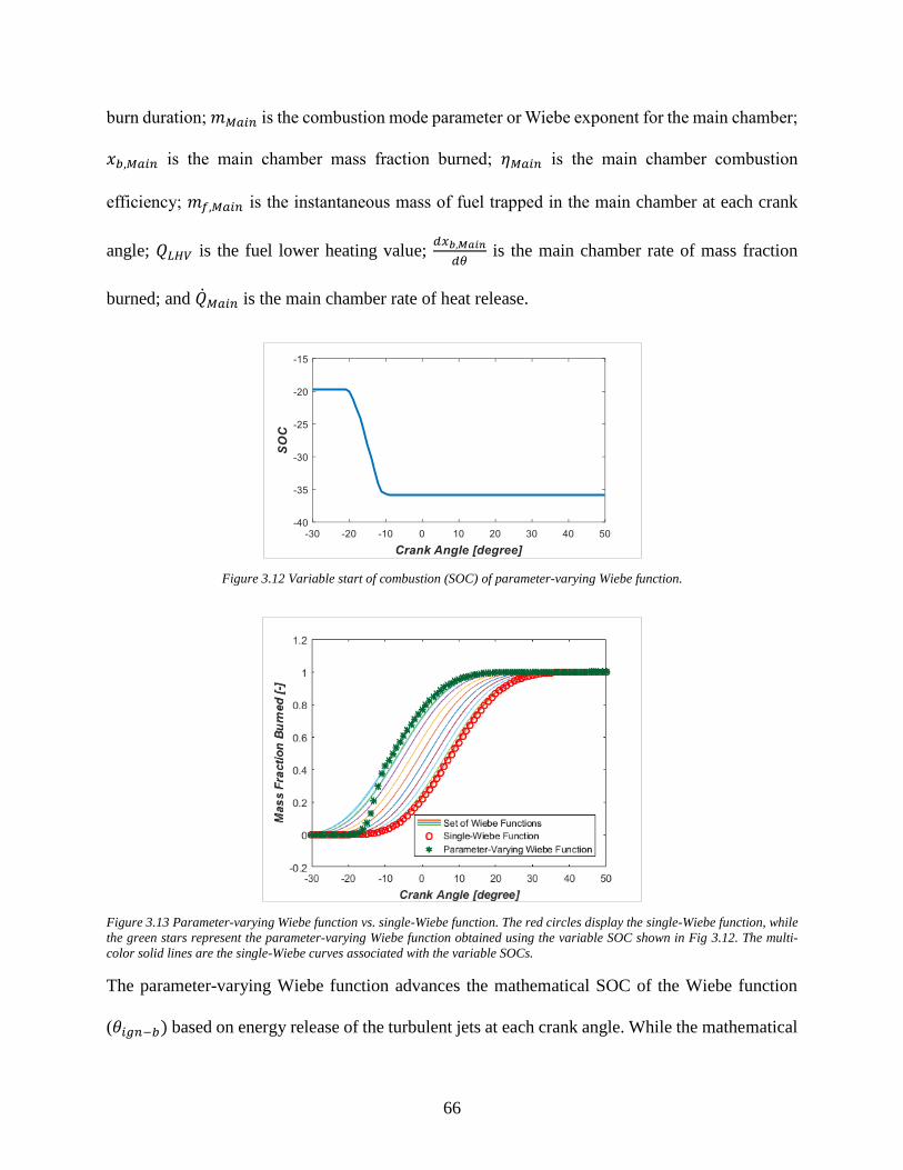
66

burn duration; 𝑚𝑀𝑎𝑖𝑛 is the combustion mode parameter or Wiebe exponent for the main chamber;

𝑥𝑏,𝑀𝑎𝑖𝑛 is the main chamber mass fraction burned; 𝜂𝑀𝑎𝑖𝑛 is the main chamber combustion

efficiency; 𝑚𝑓,𝑀𝑎𝑖𝑛 is the instantaneous mass of fuel trapped in the main chamber at each crank

angle; 𝑄𝐿𝐻𝑉 is the fuel lower heating value; 𝑑𝑥𝑏,𝑀𝑎𝑖𝑛

𝑑𝜃 is the main chamber rate of mass fraction

burned; and �̇�𝑀𝑎𝑖𝑛 is the main chamber rate of heat release.

Figure 3.12 Variable start of combustion (SOC) of parameter-varying Wiebe function.

Figure 3.13 Parameter-varying Wiebe function vs. single-Wiebe function. The red circles display the single-Wiebe function, while

the green stars represent the parameter-varying Wiebe function obtained using the variable SOC shown in Fig 3.12. The multi-

color solid lines are the single-Wiebe curves associated with the variable SOCs.

The parameter-varying Wiebe function advances the mathematical SOC of the Wiebe function

(𝜃𝑖𝑔𝑛−𝑏) based on energy release of the turbulent jets at each crank angle. While the mathematical

67

SOC is shifted, the physical SOC (𝜃0,𝑀𝑎𝑖𝑛) is kept constant with an ignition delay (∆𝜃𝑖𝑔𝑛𝐷−𝑀𝑎𝑖𝑛)

with respect to SOC inside the pre-chamber. Figure 3.12 shows a sample calculation for the

variable SOC. Figure 3.13 represents the mass fraction burned of the parameter-varying Wiebe

function using the variable SOC shown in Fig. 3.12, compared to a single-Wiebe function. The

parameter-varying Wiebe function and the single-Wiebe function shown in Fig. 3.13 have the same

physical SOC (𝜃0,𝑀𝑎𝑖𝑛). This burn dependency was imposed using available control

templates/objects on the GT-POWER platform.

3.5.2 Calibration of Engine System Model

The engine system model developed includes the detailed geometry of the pre- and main

combustion chambers, along with the intake and exhaust systems. The test cell pressure,

temperature, and relative humidity measured were set as boundary conditions for both the intake

and exhaust systems. The wall temperature of the intake port was set to 360 K which is the

temperature associated with the 50:50 ethylene glycol-water mixture through flow passages of the

engine. The wall temperature of the exhaust port was defined as 450 K at wide-open throttle and

400 K at partially throttled conditions. The heat transfer multiplier for the intake/exhaust ports was

fixed at 1.5. The wall temperatures for the intake system upstream of the intake port were assumed

to be the test cell temperature. The wall temperatures downstream from the exhaust port were

calculated using the GT-POWER wall temperature calculator.

The amount of fuel injected for the main combustion chamber was obtained by calibration of the

fuel injector at atmospheric pressure. For all the experiments, the main fuel injection happened at

-360 crank angle degree after top dead center of fire (CADaTDCF). For the calibration points at

wide-open throttle, the in-cylinder pressure at the time of main fuel injection is around atmospheric

pressure. The changes in fuel flow due to lower in-cylinder pressures for partially throttled

68

conditions were not considered in the current study. The number of fuel injections was set

according to the experiments, while the fuel profiles were linearly defined to capture the right

amount of fuel measured by the main fuel calibration. The pulse widths of the fuel injection for

the pre-chamber were within linearity limit of the fuel injector, reported by Bosch. Thus, the

amount of fuel injected was considered to be linear with the pulse width. The detailed fueling event

of the pre-chamber was explained earlier under “Pre-Chamber Evaporation Model.” The

intake/exhaust valve lifts were imposed directly, as well as the lift profile for the pre-chamber

purge assembly and spark timing. The lift profiles of the intake, exhaust, and pre-chamber purge

valves were measured using the MICRO-EPSILON optoNCDT displacement sensor, prior to the

complete engine assembly.

The developed model consists of three sets of calibrating parameters specifying the engine

combustion characteristics for both pre- and main combustion chambers; the pre-chamber fuel

evaporation; and the heat transfer and flow characteristics between pre- and main combustion

chambers. The calibrating parameters are listed in Table 3.3.

For each calibration point, the motoring pressure was closely matched to the experimental hot

motoring pressure by optimizing the heat transfer and flow calibrating parameters. The main

chamber wall temperatures of 170 ˚C, 150 ˚C, and 130 ˚C for the cylinder head, piston, and liner

respectively with a heat transfer multiplier of 1 seemed to give a good prediction of the lean

operating conditions tested in this study. The pre-chamber wall temperature was assumed to be the

same as main chamber head temperature. The heat transfer multiplier of the pre-chamber was

considered to be the same as that for the main chamber. The forward and backward discharge

coefficients for the six-hole orifice connecting the pre- to the main chamber appeared to have a

considerable effect on the correct prediction of the air flow for the pre-chamber valve assembly,

69

as well as the right motoring pressure for the pre-chamber in reference to the main chamber. The

pre-chamber pressure is slightly lower than the main chamber pressure during compression, and it

tends to reverse its behavior as combustion starts in the pre-chamber or during the expansion

stroke. The discharge coefficients were found to be 0.63 and 0.68 for forward and reverse flow,

respectively. Forward flow in this simulation is in the direction of pre- to the main chamber.

Table 3.3 Calibrating parameters including the combustion-related parameters, the evaporation parameter, and the heat transfer &

flow parameters.

Combustion Calibrating Parameters

𝜷 [-] Calibrating parameter to maintain the burn dependency of the pre- to the main chamber

𝜶𝑷𝒓𝒆 [-] Pre-chamber ignition delay calibrating parameter

𝒎𝒑𝒓𝒆 [-] Combustion mode parameter or Wiebe exponent for the pre-chamber

∆𝜽𝑷𝒓𝒆 [CAD] Total burn duration for the pre-chamber

𝜶𝑴𝒂𝒊𝒏 [-] Main chamber ignition delay calibrating parameter

𝒎𝑴𝒂𝒊𝒏 [-] Combustion mode parameter or Wiebe exponent for the main chamber

∆𝜽𝑴𝒂𝒊𝒏 [CAD] Total burn duration for the main chamber

𝜼𝒆𝒇𝒇−𝑷𝒓𝒆 [%] Combustion efficiency of the pre-chamber

𝜼𝒆𝒇𝒇−𝑴𝒂𝒊𝒏 [%] Combustion efficiency of the main chamber

Evaporation Calibrating Parameter

𝒌 [-] Fraction of fuel to be evaporated at the time of injection into the pre-chamber

Heat Transfer and Flow Calibrating Parameters

𝑪𝒅𝒇𝒘𝒅 [-] Forward discharge coefficient for six-hole orifice connecting the pre- to the main chamber

𝑪𝒅𝒃𝒌𝒘 [-] Backward discharge coefficient for six-hole orifice connecting the pre- to the main chamber

𝑻𝒉𝒆𝒂𝒅− 𝑴𝒂𝒊𝒏 [C] Main chamber head temperature

𝑻𝒑𝒊𝒔𝒕𝒐𝒏− 𝑴𝒂𝒊𝒏 [C] Main chamber piston temperature

𝑻𝒍𝒊𝒏𝒆𝒓− 𝑴𝒂𝒊𝒏 [C] Main chamber liner temperature

𝑻𝒘𝒂𝒍𝒍− 𝑷𝒓𝒆 [C] Pre-chamber wall temperature

𝑯𝑻𝑴𝑷𝒓𝒆 [-] Pre-chamber heat transfer multiplier

𝑯𝑻𝑴𝑴𝒂𝒊𝒏 [-] Main chamber heat transfer multiplier

The single calibrating parameter for the pre-chamber evaporation modeling was previously

optimized with the combustion-related calibrating parameters at 1500 rpm with a wide-open

throttle. Different scenarios were studied, as the “k” factor ranged from 0.66 to 0.75. It appeared

that a “k” factor of 0.7 is sufficiently precise for the optimization performed. The primary fuel

injection event into the pre-chamber starts within 1 CAD of the end of the pre-chamber purge valve

closing, for the cases studied. The upstream pressure and temperature of the purge valve were kept

constant during the experiments. Although characteristics of the air trapped in the pre-chamber at

the time of fuel injection may vary at different loads and speeds, the effect of associated variations

70

on the “k” factor was considered negligible in regard to the precision expectancy of the 0D/1D

model developed. A “k” factor of 0.7 was used through the entire simulation, which is equivalent

to 70% of the fuel injected into the pre-chamber being evaporated at the time of injection.

The main chamber total burn duration, the pre-chamber combustion efficiency, and the main

chamber combustion efficiency were pre-determined. The pre-chamber combustion mode

parameter, Wiebe exponent, was also closely restricted to a narrow range of valid values. The pre-

determination of some of the parameters is necessary when the cost function is co-dependent on a

group of calibrating parameters. This co-dependency leads to the compensation by a number of

parameters if any shortage of the cost function appears with respect to the rest of the calibrating

parameters. The main chamber total burn duration is set to 60 CAD, while the pre- and main

combustion efficiencies were assumed as 98%. The remaining calibrating parameters were

optimized using a nondominated sorting genetic algorithm (NSGA).

The nondominated sorting genetic algorithm III (NSGA-III) [108] used in this simulation is the

successor to NSGA-II and is optimized for multi-objective Pareto optimization. NSGA-III is a

powerful global optimizer for a thorough search of the entire design space. There are two main

inputs to be defined prior to a NSGA optimization: the population size and the number of

generations. There are recommendations available based on the number of parameters to be

calibrated. A population size of 26 was chosen for the current study, having 6 calibrating

parameters to be optimized at the same time. The number of generations was observed to be 20±5

to reach a reasonable convergence.

A cost (fitness) function was defined to include the weighted summation of squared numerical-to-

experimental errors for both pre- and main combustion chambers during the pre-chamber

combustion before top dead center of fire (TDCF); the weighted squared numerical-to-

71

experimental error for the amplitude and phasing of the main chamber maximum pressure; and the

weighted squared numerical-to-experimental errors for five selected points from the main chamber

pressure trace. The weighting factors were studied to improve the cost function toward capturing

the right pressure traces for both pre- and main combustion chambers. Equation 3.16 displays the

cost function used in this study.

𝐶𝑜𝑠𝑡 𝐹𝑢𝑛𝑐𝑡𝑖𝑜𝑛 =

∑ {𝑤1(𝑝𝑁𝑢𝑚,𝑃𝑟𝑒 − 𝑝𝐸𝑥𝑝,𝑃𝑟𝑒)2

+ 𝑤2(𝑝𝑁𝑢𝑚,𝑀𝑎𝑖𝑛 − 𝑝𝐸𝑥𝑝,𝑀𝑎𝑖𝑛)2

}𝑃𝑟𝑒𝐶ℎ

𝐶𝑜𝑚𝑏𝑢𝑠𝑡𝑖𝑜𝑛

+

𝑤3(𝑝𝑁𝑢𝑚 − 𝑝𝐸𝑥𝑝)𝑀𝑎𝑥 𝐴𝑚𝑝𝑙𝑖𝑡𝑢𝑑𝑒,𝑀𝑎𝑖𝑛

2+

𝑤4(𝜃𝑁𝑢𝑚 − 𝜃𝐸𝑥𝑝)𝑀𝑎𝑥 𝐴𝑚𝑝𝑙𝑖𝑡𝑢𝑑𝑒,𝑀𝑎𝑖𝑛

2+

∑ 𝑤𝑖+4(𝑝𝑁𝑢𝑚 − 𝑝𝐸𝑥𝑝)𝑃𝑜𝑖𝑛𝑡 𝑖,𝑀𝑎𝑖𝑛

25

𝑖=1

(3.16)

where, 𝑤1 to 𝑤9 are the weighing factors for the terms defined in the cost function, 𝑝 is the in-

cylinder pressure, and 𝜃 is the instantaneous crank angle degree. Subscripts “𝑃𝑟𝑒”, “𝑀𝑎𝑖𝑛”,

“𝑁𝑢𝑚”, and “𝐸𝑥𝑝” denote the pre-chamber, main chamber, numerical, and experimental;

respectively.


3.6.1 Energy Input for a Pre-Chamber Air Valve

The dampener system, explained under “Experimental Setup” and shown in Fig. 3.7, successfully

dampened the flow upstream of the air valve for a reliable flow measurement. Figure 3.14 shows

the flow measured by the low-range laminar flow element (LFE) at 1500 rpm with a wide-open

throttle (WOT). The volume flow fluctuation is negligible considering that the flow upstream of

the air valve is highly pulsatile. As seen in Fig. 3.14, the average flow slightly decreases over time.

The downward trend, although small, may be due to the wall temperature rise of the pre-chamber.

72

A comprehensive study is needed to find the elements involved and their corresponding effects.

The average volume flow rate was observed to be 0.15 SCFM at 1500 rpm. At 2000 rpm, the

average flow was measured as 0.16 SCFM which is slightly higher than the flow at 1500 rpm. The

pre-chamber air valve was opened at -150 CADaTDCF and closed at -120 CADaTDCF with 1 bar

gauge upstream pressure.

Figure 3.14 Volume flow rate measured by the low range LFE at 1500 rpm with a WOT.

The LFE reading was verified by direct measurement using a displaced bubble technique as well

as by GT-POWER Model, with the results found to be in good agreement. The purge valve flow

coefficients were adjusted accordingly along with the discharge coefficients of the six-hole orifice,

connecting the pre- to the main chamber, to replicate the experimental data. Numerical results for

the pre-chamber air flow precisely follow the experiments for both 1500 rpm and 2000 rpm. The

relative error was below 2% of the experimental data.

Based on the results obtained in the Prototype II DM-TJI engine and the Womack fluid power

design sheet [109], at 1 bar gauge upstream pressure less than 6.5 watts of power are required to

deliver 0.15 SCFM or 0.16 SCFM air flow; corresponding to 1500 rpm and 2000 rpm, respectively.

Thus, for a four-cylinder engine running at 1500 rpm or 2000 rpm, 25 watts of power would be

sufficient. At higher speeds and loads or under highly dilute conditions, the required airflow will

Average: 0.15 SCFM

73

be greater. However, by delivering the pre-chamber air during the appropriate time of

compression, work will be recovered from the pre-chamber purge air during the expansion stroke

of the piston.

In addition to pumping air, the work required to activate the valve system for a four-cylinder engine

is about 75 watts at 2000 RPM. This value is based on power requirements to drive an engine

camshaft given to MSU from a Tier 1 OEM supplier. The DM-TJI system has a small poppet valve

with a small actuation lift requirement. The assumption of 75 watts is very conservative. It is half

of the power required for a conventional camshaft. Mechanical cams are extremely efficient valve

actuators, as the compressed springs put work back into the system during decompression.

It appears that this function is ideally suited to electrification, as the trend in the next decade is that

nearly all vehicles will be at least partially electrified. If a pre-chamber reservoir is charged at a

condition where excess electrical energy is available, either because a battery is fully charged or

can only take charging at a certain rate, that energy to drive the electric pump is actually free.

Results to date show that power consumption to deliver pre-chamber air will not be a factor

limiting implementation of the technology.

3.6.2 Combustion Stability

An extensive set of experiments was conducted on the Prototype II DM-TJI engine. The

experiments were run at 1500 rpm and 2000 rpm with both wide-open throttle (WOT) and the

throttle partially opened. The normalized air/fuel ratio (lambda) was kept at 1.9±0.1 for all the

experiments in this study. The spark timing and the fuel strategy in the pre-chamber were varied

to obtain the combustion stability at each operating condition. The fueling event of the pre-

chamber happened at -120 CADaTDCF with one pulse of 1.3 ms or 1.5 ms. Table 3.4 summarizes

74

the spark sweeps and the fuel strategies examined in this study. The pre- and main chamber fuel

injectors were run at 100 bar with 3 pulses of fuel into the main chamber starting at -360

CADaTDCF with 1.5 ms in between. The pre-chamber air valve was opened at -150 CADaTDCF

and closed at -120 CADaTDCF with 1 bar gauge upstream pressure.

Table 3.4 Spark sweeps and fuel strategies associated with the points examined in this study.

Speed

[rpm]

Throttle Position

[-]

Spark Sweep

[CADaTDCF]

Pre-Chamber

Fuel Strategy

[ms]

2000 Wide Open -29, -28, -27, -26 1.3, 1.5

2000 Partial -36, -34 1.3, 1.5

1500 Wide Open -29, -28, -27, -26, -25 1.3, 1.5

1500 Partial -34, -33, -32, -31 1.3, 1.5

Results demonstrated a stable combustion for all four operating conditions over the spark sweep

and the two fuel strategies inside the pre-chamber. Combustion stability with an IMEP COV below

2.5% is proven to be attained at highly lean conditions, lambda ~2, for the throttle conditions both

wide and partially opened. The observed CA50s, crank angle degree at which 50% of the fuel is

burned, ranged from 3 to 6 CADaTDCF.

3.6.3 Brake Efficiency Calculation

A preliminary efficiency calculation was conducted on the results obtained from experiments

under highly lean conditions, lambda ~2. A friction loss of 6% with no pumping loss at WOT and

a 3% pumping loss at partially throttled conditions were considered in these calculations. An

estimation of the work input for the air valve assembly, as explained under “Energy Input for a

Pre-Chamber Air Valve,” was included in the brake efficiency calculations. The lower heating

value of the fuel used in this study was examined and reported by Galbraith Laboratories Inc. as

43.2 MJ/kg.

The case at 2000 rpm with a WOT maintained the highest gross indicated efficiency at 41.2%,

which resulted in 38.6% brake thermal efficiency. The second-highest gross indicated efficiency

75

belonged to the case at 1500 rpm with a WOT at 40.3%. The brake thermal efficiency was then

calculated as 37.6%. The operating conditions with partially opened throttle at 2000 rpm and 1500

rpm resulted in 39.8% and 40.1% of gross indicated efficiencies, leading to 36.1% and 36.2% in

brake thermal efficiencies, respectively.

Table 3.5 presents the efficiency calculations. The thermal efficiencies obtained for the Prototype

II DM-TJI engine were compared to the results reported by Ortiz-Soto and colleagues for an engine

run under an advanced multi-mode combustion in Fig. 3.15. The multi-mode combustion studied

in their work involved spark ignition (SI), homogeneous charge compression ignition (HCCI), and

spark-assisted compression ignition (SACI) operating strategies [107]. The SI-HCCI-SACI engine

used in their study has the same bore and stroke (86 mm/94.3 mm) as the DM-TJI engine examined

in the current work, with slightly higher compression ratio (12.42:1) than the Prototype II DM-TJI

engine. Figure 3.15 clearly demonstrates the potential of a DM-TJI system for higher thermal

efficiencies at low to mid-load operating conditions, as the results obtained for the DM-TJI system

lie close to those for HCCI-SACI combustion. The DM-TJI system benefits from high thermal

efficiencies close to HCCI-SACI combustion technologies, while it does not involve the

difficulties arising from those types of combustion. The latter difficulties include the complex

control mechanism and fuel intolerance.

Table 3.5 Preliminary brake efficiency calculations for the Prototype II DM-TJI engine (naturally aspirated, CR=12:1, bore=86

mm, stroke=95 mm). A friction loss of 6% with no pumping loss at WOT and a 3% pumping loss at partially throttled conditions

were considered in these calculations. The work input associated to the pre-chamber air valve was included proportional to the

volume flow rate of the pre-chamber air valve.

Speed

[rpm]

Throttle

Position

[-]

Gross

IMEP

[bar]

BMEP,

WO Pre Air

[bar]

BMEP,

W Pre Air

[bar]

Gross

Indicated

Efficiency

[%]

Brake

Efficiency,

WO Pre Air

[%]

Brake

Efficiency,

W Pre Air

[%]

2000 WOT 6.60 6.20 6.18 41.2 38.8 38.6

2000 Partial 4.47 4.08 4.05 39.8 36.3 36.1

1500 WOT 6.04 5.68 5.64 40.3 37.9 37.6

1500 Partial 4.54 4.14 4.10 40.1 36.5 36.2

76

Figure 3.15 Thermal efficiencies obtained for the Prototype II DM-TJI engine compared to an engine run under SI-HCCI-SACI

combustion strategies. The main figure is a duplication of the results presented by Ortiz-Soto and colleagues in “Thermodynamic

efficiency assessment of gasoline spark ignition and compression ignition operating strategies using a new multi-mode combustion

model for engine system simulations” [107]. The data from the Prototype II DM-TJI were added based on preliminary efficiency

calculations under lean operating conditions, lambda ~2.

3.6.4 Model Predictions of Experimental Trends

The engine system model developed was calibrated based on experimental data at four operating

conditions shown in Table 3.5. The calibration processes were explained previously under

“Calibration of Engine System Model,” and the results are presented in Table 3.6. In general, it

appears that the numerical simulations were able to capture the experimental trends. The validity

of the model in prediction of experiments was observed based on the standard metric of the

coefficient of determination, 𝑅2, shown in Fig. 3.16; and comparison plots for the in-cylinder

pressures presented in Figs. 3.17, 3.18, 3.19, and 3.20. The dashed lines in Fig. 3.16 indicate 5%

error lines. Numerical predictions for three metrics of main chamber combustion (gross IMEP,

main chamber peak pressure, and main chamber phasing for the peak pressure) were within 5% of

experimental data with one exception happening at 6% (peak pressure phasing of the main chamber

for partially throttled case at 1500 rpm). Solid blue lines in the upper images of Figs. 3.17-3.20

77

represent the experimental trend, while numerical predictions are depicted in dashed red lines. The

lower images in the same figures show the numerical-to-experimental errors at each crank angle.

The absolute root mean square (RMS) errors of in-cylinder pressures for both pre- and main

combustion chambers were below 0.35.

Table 3.6 Optimization results for the calibrating parameters of the engine system model.

2000/WOT 2000/PT 1500/WOT 1500/PT


𝛽 [-] 0.88 1.08 1.05 0.62

𝑃𝑟𝑒𝐶h 𝐼𝑔𝑛𝑖𝑡𝑖𝑜𝑛 𝐷𝑒𝑙𝑎𝑦 𝐼𝑛𝑑𝑒𝑥 [-] 0.19 0.24 0.18 0.20

𝑚𝑝𝑟𝑒 [-] 0.51 0.50 0.56 0.50

∆𝜃𝑃𝑟𝑒 [CAD] 47.23 45.03 50.70 45.56

𝑀𝑎𝑖𝑛𝐶h 𝐼𝑔𝑛𝑖𝑡𝑖𝑜𝑛 𝐷𝑒𝑙𝑎𝑦 𝐼𝑛𝑑𝑒𝑥 [-] 0.17 0.18 0.10 0.11

𝑚𝑀𝑎𝑖𝑛 [-] 2.73 2.50 2.95 2.35

∆𝜃𝑀𝑎𝑖𝑛 [CAD] 60.00 60.00 60.00 60.00

𝜂𝑒𝑓𝑓−𝑃𝑟𝑒 [%] 98.00 98.00 98.00 98.00

𝜂𝑒𝑓𝑓−𝑀𝑎𝑖𝑛 [%] 98.00 98.00 98.00 98.00


𝑘 [-] 0.7 0.7 0.7 0.7


𝐶𝑑𝑓𝑤𝑑 [-] 0.63 0.63 0.63 0.63

𝐶𝑑𝑏𝑘𝑤 [-] 0.68 0.68 0.68 0.68

𝑇ℎ𝑒𝑎𝑑− 𝑀𝑎𝑖𝑛 [C] 170 170 170 170

𝑇𝑝𝑖𝑠𝑡𝑜𝑛− 𝑀𝑎𝑖𝑛 [C] 150 150 150 150

𝑇𝑙𝑖𝑛𝑒𝑟− 𝑀𝑎𝑖𝑛 [C] 130 130 130 130

𝑇𝑤𝑎𝑙𝑙− 𝑃𝑟𝑒 [C] 170 170 170 170

𝐻𝑇𝑀𝑃𝑟𝑒 [-] 1 1 1 1

𝐻𝑇𝑀𝑀𝑎𝑖𝑛 [-] 1 1 1 1

Figure 3.16 Correlation plots for gross IMEP, main chamber peak pressure, and peak pressure phasing of the main chamber. The

high 𝑅2 values indicate the high level of correlation between numerical predictions and experiments.

78

Figure 3.17 Model prediction vs. experiments for in-cylinder pressures of pre- and main combustion chambers at 2000 rpm with a

WOT.


throttle partially opened.


WOT.

79


throttle partially opened.

As mentioned earlier, none of the studies to date on the DM-TJI engine predicted the losses of

such a system. Table 3.7 presents the heat transfer and exhaust losses as the percentage of total

fuel energy in addition to the pre-chamber lambda at the time of spark timing, and the main

chamber combustion phasing and 10-90% burn duration. Model prediction for ignition delays of

pre- and main combustion chambers are also shown in the same table.

Table 3.7 Model prediction of in-cylinder characteristics.

2000/WOT 2000/PT 1500/WOT 1500/PT

Pre-Chamber Lambda @Spark Timing 1.2 0.7 1.0 0.8

Main Chamber CA50* [CADaTDCF] 6.5 2.9 4.3 3.1

Burn 10-90** [CAD] 26.1 26.4 25.3 26.7

Pre-Chamber Ignition Delay [CAD] 4.86 8.56 4.81 6.36

Main Chamber Ignition Delay [CAD] 4.39 6.44 2.71 3.48

Heat Transfer, % of Total Fuel Energy 22.3 25.5 26.0 28.4

Exhaust, % of Total Fuel Energy 35.3 34.9 32.8 32.6

Indicated Efficiency, % of Total Fuel Energy 41.2 39.6 41.2 39.0

* The crank angle degree at which 50% of the fuel is burned.

** The duration in crank angle degree from 10% of the fuel burned to the 90%.

The results demonstrate a range of lambda distribution for the pre-chamber at the time of spark

event, from slightly rich (lambda <1) to slightly lean (lambda > 1). The results may be in part

influenced by pre-chamber evaporation modeling which considers a fixed percentage of fuel

evaporation at the time of fuel injection into the pre-chamber. However, the range of lambda

distributions obtained is within the range described for this type of combustion technology

[47,52,53], with previous studies being more inclined toward the rich side of air/fuel ratios.

80

The CA50 values calculated for the main combustion chamber ranged from 3 to 6 CADaTDCF.

The 10-90% burn duration ranged from 25 to 27 CAD. Ortiz-Soto and colleagues reported the 10-

90% burn duration ranging from 25 to 28 CAD for their idealized-air and idealized-EGR

simulations [107], while the combustion efficiency was considered as ~98%. Such idealized

simulations were corresponding to 40-45% gross thermal efficiencies. The 10-90% burn durations

for HCCI-SACI combustion have been also reported by the same group in the range of 5 CAD to

20 CAD, with combustion efficiency ranging from 85% to 98%. As the thermal efficiencies for

the DM-TJI system were close to those in HCCI-SACI combustion reported by Ortiz-Soto et al.,

one may expect the same in-cylinder behaviors as well. In this study, the combustion efficiency of

the DM-TJI engine was assumed as 98% for both pre- and main combustion chambers. However,

a lower combustion efficiency will lead to a faster burn rate calculation for the DM-TJI system, as

both HCCI-SACI and DM-TJI engines benefit from the same high thermal efficiencies. Further

studies should be conducted to shed light on this matter.

The simple approach employed to capture ignition delays for both pre- and main combustion

chambers seems to predict a reasonable trend. As described earlier under “Numerical Approach

and Model Development,” two calibrating parameters (𝛼𝑃𝑟𝑒 and 𝛼𝑀𝑎𝑖𝑛) were optimized at each of

the four operating conditions studied here to define ignition delays of the pre- and main chambers.

These two parameters were normalized with respect to spark timing. The results obtained

demonstrated an increase in ignition delays as the engine speed increases, and a decrease in ignition

delays as the load increases. The trend observed is in agreement with the results reported by

Assanis and colleagues [36] for the ignition delays of a direct-injection diesel engine. Tolou and

colleagues observed the same trend for ignition delays of a gasoline direct injection (GDI) engine

81

[110]. However, the former study reported an increase in ignition delays, as the load further

increases and exceeds 120 N-m of brake torque at high-boost conditions.

Model prediction for in-cylinder losses toward the heat transfer and exhaust follows a logical trend.

Heat transfer decreases, as engine speed increases. Energy loss through exhaust, on the other hand,

increases, as engine speed goes up. The rise in exhaust energy loss at higher speeds seems

reasonable, as not all the energy saved by less heat transfer at higher speeds will be recovered as

indicated efficiencies. On average, 26% of total fuel energy is lost through heat transfer, followed

by 34% through exhaust. The averaged loss mentioned above leaves a 40% indicated thermal

efficiency at low to mid-load operating conditions for the DM-TJI system examined in the current

work.

3.6.5 Predictive, Generalized Model for a DM-TJI Engine

The optimization results for model calibrating parameters were further studied to propose a

predictive, generalized model for a DM-TJI engine. Such a model is essential to project the

behavior of an engine equipped with the DM-TJI combustion technology over the entire engine

fuel map. Table 3.6 presented the optimization results for each of the calibrating parameters in this

study. Considering the low range of variation for each of these parameters, it seems that an average

value should well predict the general behavior. The combustion-related calibrating parameters,

optimized by NSGA and described in Table 3.6, were averaged over the four cases examined in

this study. The parameters recommended for a predictive, generalized model are listed in Table

3.8.

The author proposes that the spark timing should be optimized at each operating condition to

achieve the highest thermal efficiency, while the 10-90% burn duration is kept below 27 CAD. In

82

this study, the highest 10-90% burn duration was observed to be 27 CAD. Lavoie and colleagues

reported a 10-90% burn duration of 25 CAD as a choice to obtain best efficiencies possible over

the range of conditions studied [111]. The 25 CAD of 10-90% burn duration was described by the

same group as the mid-way between HCCI and dilute SI combustion. The study by Lavoie et al.

also determined a minimum 10-90% burn duration of ~20 CAD as the low limit to achieve high

efficiencies in normal engines with heat transfer. The gain in thermal efficiency by further

reduction of 10-90% burn duration below 20 CAD was perceived to be negligible.

Table 3.8 Calibrating parameters for a predictive, generalized model of a DM-TJI system.


𝛽 [-] 0.9

𝑃𝑟𝑒𝐶h 𝐼𝑔𝑛𝑖𝑡𝑖𝑜𝑛 𝐷𝑒𝑙𝑎𝑦 𝐼𝑛𝑑𝑒𝑥 [-] 0.20

𝑚𝑝𝑟𝑒 [-] 0.5

∆𝜃𝑃𝑟𝑒 [CAD] 47

𝑀𝑎𝑖𝑛𝐶h 𝐼𝑔𝑛𝑖𝑡𝑖𝑜𝑛 𝐷𝑒𝑙𝑎𝑦 𝐼𝑛𝑑𝑒𝑥 [-] 0.14

𝑚𝑀𝑎𝑖𝑛 [-] 2.6

∆𝜃𝑀𝑎𝑖𝑛 [CAD] 60.00

𝜂𝑒𝑓𝑓−𝑃𝑟𝑒 [%] 98.00

𝜂𝑒𝑓𝑓−𝑀𝑎𝑖𝑛 [%] 98.00


𝑘 [-] 0.7


𝐶𝑑𝑓𝑤𝑑 [-] 0.63

𝐶𝑑𝑏𝑘𝑤 [-] 0.68

𝑇ℎ𝑒𝑎𝑑− 𝑀𝑎𝑖𝑛 [C] 170

𝑇𝑝𝑖𝑠𝑡𝑜𝑛− 𝑀𝑎𝑖𝑛 [C] 150

𝑇𝑙𝑖𝑛𝑒𝑟− 𝑀𝑎𝑖𝑛 [C] 130

𝑇𝑤𝑎𝑙𝑙− 𝑃𝑟𝑒 [C] 170

𝐻𝑇𝑀𝑃𝑟𝑒 [-] 1

𝐻𝑇𝑀𝑀𝑎𝑖𝑛 [-] 1

As the pre-chamber combustion is the source of ignition inside the main chamber, the pre-chamber

fuel, and the pre-chamber air valve timing and upstream pressure should also be optimized at each

operating condition to maintain a lambda of 0.9±5% at the time of spark event. The 0.9 lambda is

the 4-case- averaged value of the model predictions at the time of spark timing. The 5% bandwidth

was defined to account for the uncertainties regarding the lambda calculation. Maintaining a proper

lambda at the time of spark event will be more crucial if the model is used to project the behavior

83

of the DM-TJI engine under highly dilute conditions with excess EGR. Based on the Womack

fluid power design sheet [109], the work required to deliver air to the pre-chamber of a DM-TJI

system is proportional to both pressure and volume flow rate. These differ from one operating

condition to another. Furthermore, the primary fueling event inside the pre-chamber should always

happen within a small number of crank angle degrees from the pre-chamber valve closing to

maintain the stoichiometry inside the pre-chamber.

The in-cylinder maximum pressures can be limited by adding a constraint to the optimization to

reflect the design specifications. Wall temperatures of pre- and main combustion chambers may

also need to be modified based on an engineering judgment at higher loads.

The possibility of knocking behavior, which is more likely to happen at low speeds and high loads,

was not examined in the current study. This issue is not considered as an error to the current

modeling approach, but as a limitation of the current analysis. Investigating the knocking behavior

was out of the scope of the current project and its experimental platform. Thus, if it were possible

to address the knocking behavior by any means including but not limited to in-cylinder charge

preparation and/or combustion chamber design, the current model should be capable of projecting

the DM-TJI engine behavior over the entire engine fuel map.

3.6.6 DM-TJI Engine Fuel Map under Highly Dilute Conditions

The approach described above was utilized to generate a complete engine fuel map which covers

the power requirements of the Ford F-150 2.7-Liter EcoBoost®. According to the National Public

Radio (NPR), a Ford F-150 pickup truck is sold about every 30 seconds in the U.S. [112]. The

Ford F-150 is not only America’s best-selling pickup truck but also America’s best-selling vehicle

84

in total [113]. The Ford F-Series has gained an incredible reputation in both fuel economy and

vehicle performance.

The Ford 2.7-Liter EcoBoost® is a turbocharged six-cylinder engine which includes the Ford port-

fuel and direct-injection (PFDI) system with two injectors per cylinder; dual overhead cam design

with variable intake/exhaust cam timing; and twin intercooled turbochargers for on-demand power

[114]. The maximum torque curve of the engine was satisfied via a four-cylinder boosted

configuration of the DM-TJI engine with higher limits for brake mean effective pressures (BMEP).

A maximum of 2 bar gauge boost pressure and 40% exhaust gas recirculation (EGR) were

employed. The in-cylinder pressures for both pre- and main combustion chambers were bound to

a maximum of 150 bar at high-load operating conditions.

Figure 3.21 presents a conceptual diagram for the modeling framework used in this study in order

to generate a full engine map, equivalent to power requirements of the Ford F-150 2.7-Liter

vehicle. The black solid line in this figure shows the maximum torque curve for the 2.7-Liter

EcoBoost® engine. The full fuel map of the 2.7-Liter EcoBoost® was produced by the U.S. EPA

National Vehicle and Fuel Emission Laboratory (NVFEL) located in Ann Arbor, Michigan

[115,116]. The dash-dot line in grey marks the naturally aspirated line at 40% external EGR. The

core data including the ones representing the naturally aspirated line up to the maximum torque

curve were generated by the GT-POWER model simulations performed in the current study. As

one can see in Fig. 3.21, the external EGR was first kept constant, while the boost pressure was

increased to achieve higher loads at different speeds. After that, the boost pressure was kept

constant at 2 bar gauge (maximum boost pressure used in the current simulations) and the amount

of external EGR was reduced to reach the maximum torque of 508.4 N-m at 3000 rpm.

85

At each operating condition, the main chamber fuel was first optimized to maintain the

stoichiometry for the rest of the charge trapped in the cylinder. Afterward, a GA optimization was

run for each of the operating conditions to optimize the spark timing, the pre-chamber fuel, and

the pre-chamber valve upstream pressure and timing. The goal of the optimization was defined to

maximize the indicated gross efficiency. The maximum in-cylinder pressures of 150 bar and the

pre-chamber lambda of 0.9±5% at the time of spark event were added as constraints to the

optimizations. The amount of EGR trapped in the pre-chamber at start of combustion (SOC) was

also constrained to a maximum of 30% to ensure a successful combustion in the pre-chamber. The

optimizations were performed with a population size of 16, while the number of generations was

set to 5.

Figure 3.21 Modeling framework used in order to generate a full engine map, equivalent to the power requirements of the Ford F-

150 2.7-Liter EcoBoost®, for the DM-TJI engine under highly dilute conditions.

GT-POWER

Scaled 2.7-Liter EcoBoost®

2 barG Boost, 0% EGR





1.5 barG Boost, 40% EGR


0.5 barG Boost, 40% EGR

NA, 40% EGR

86

The core data below the naturally aspirated line were covered based on experimental data from the

2.7-Liter EcoBoost® at a number of brake mean effective pressures (BMEP) in that region. The

fuel consumptions of the 2.7-Liter EcoBoost® at low loads were scaled to be used toward the fuel

map generation of the DM-TJI engine. The data scaling took place using Equation 3.17 with taking

into account the change in engine displacement from the 2.7-Liter EcoBoost® to the 2.2-Liter DM-

TJI engine. The 2.7-Liter EcoBoost® includes 6 cylinders of 0.45-Liter, while the DM-TJI engine

was defined in a four-cylinder configuration of 0.55-Liter each. The brake specific fuel

consumptions (BSFC) at each particular BMEP were kept the same. The power value, however,

reflected the change in engine displacement at the same BMEP from one engine to the other.

�̇�𝑓𝑢𝑒𝑙 (𝑔

ℎ𝑟) = 𝐵𝑆𝐹𝐶 (

𝑔

𝑘𝑊 − ℎ𝑟) × 𝑃(𝑘𝑊) (3.17)

Figure 3.22 represents the thermal efficiency map for the DM-TJI engine in a four-cylinder

configuration. Accordingly, the brake specific fuel consumption (BSFC) map in g/kW-hr is shown

in Fig. 3.23. The core data obtained from the GT-POWER simulations and the 2.7-Liter

EcoBoost® engine are displayed in black dots through the whole map for both the thermal

efficiency and BSFC. A MATLAB surface generator algorithm called “gridfit” was employed to

build the complete map of the DM-TJI engine out of obtained scattered data [117]. The smoothing

parameter of the algorithm was altered to slightly smoothen the data and achieve a better

representation. The details of BSFC calculations for the core data generated by the GT-POWER

model simulations can be found in Appendix A, Tables A.1 and A.2.

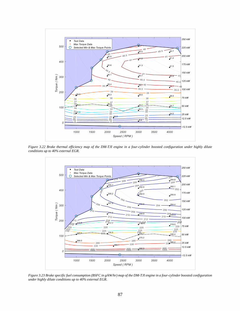
87

Figure 3.22 Brake thermal efficiency map of the DM-TJI engine in a four-cylinder boosted configuration under highly dilute

conditions up to 40% external EGR.

Figure 3.23 Brake specific fuel consumption (BSFC in g/kW/hr) map of the DM-TJI engine in a four-cylinder boosted configuration

under highly dilute conditions up to 40% external EGR.

88

The friction term in BMEP calculations of the core data generated by the GT-POWER model was

described by the Chen-Flynn equation [118], Equation 3.18.

𝐹𝑀𝐸𝑃 = 0.3 [𝑏𝑎𝑟] + 0.004 [−] 𝑃𝐶𝑦𝑙,𝑚𝑎𝑥 + 0.08 [𝑏𝑎𝑟𝑚

𝑠⁄] 𝑈𝑝 (3.18)

where, FMEP is the friction mean effective pressure in bar; 𝑃𝐶𝑦𝑙,𝑚𝑎𝑥 is the maximum cylinder

pressure in bar; and 𝑈𝑝 is the mean piston speed in m/s. Equation 3.18 includes the GT-POWER

recommended coefficients for such a model. The units for each of the coefficients in Equation 3.18

are shown in the brackets above.

Additionally, the warmed-up closed-throttle (CT) BMEP curve for the 2.7-Liter EcoBoost®

engine was provided to the MSU Energy and Automotive Research Lab (EARL) by the U.S. EPA

NVFEL. Figure 3.24 displays the segmented closed-throttle curve at four different speeds (1000

rpm to 4000 rpm with a 1000 rpm increment) compared to the FMEP results obtained by the Chen-

Flynn model for all the loads studied at the same speeds. The differences observed between the

CT values and the Chen-Flynn simulations include the slight pumping work at closed throttle plus

the energy loss through heat transfer. The maximum amount of difference was observed to be 33%

at the lowest BMEP and the speed of 2000 rpm. The minimum difference of 6% happened at the

high load and 3000 rpm. In general, the discrepancy between two curves decreases as the load

increases; and the Chen-Flynn model takes into account the term for maximum in-cylinder

pressures. The magnitude of highest relative difference between the CT values and the Chen-Flynn

calculations also decreases, as speed increases and consequently the engine heat transfer reduces.

Moreover, the discrepancy between the CT values and the Chen-Flynn model calculations

becomes almost constant, as the BMEP passes a particular threshold at higher loads. Recall that

the in-cylinder pressures for both pre- and main combustion chambers were bound to a maximum

89

of 150 bar at high-load operating conditions. The details of friction calculations for the core data

obtained by the GT-POWER model can be found in Appendix A, Table A.4. Friction calculations

performed by the Chen-Flynn equation were used toward BSFCs, as there was no other data

available on the friction curve of the 2.7-Liter EcoBoost® engine.

Figure 3.25 displays indicated gross efficiencies obtained for the current simulations with respect

to BMEP at different speeds. In general, indicated efficiency increases, as engine speed goes up.

Additionally, higher BMEPs corresponding to higher boost pressures lead to higher gross indicated

efficiencies. The indicated efficiency decreases with further increase in BMEP above 23 bar. To

obtain BMEPs above 23 bar, the in-cylinder charge dilution was reduced, and the spark timing was

retarded to not exceed the 150 bar threshold of in-cylinder pressures.

Figure 3.24 Segmented warmed-up closed-throttle (CT) BMEP curve of the 2.7-Liter EcoBoost® engine compared to the FMEP

results obtained by the Chen-Flynn model at different loads and speeds.

90

Figure 3.25 Gross indicated efficiency with respect to BMEP. The dash-dot line displays the 23 bar BMEP. The loads beyond this

point were obtained by reducing the charge dilution, while the spark timings were retarded to maintain the 150 bar constraint for

in-cylinder pressures.

Figure 3.26 Gross indicated efficiency with respect to CA50. The data report an average CA50 of 7.6 CADaTDCF as the optimum

CA50 for the current simulations performed on the DM-TJI engine. The data with retarded spark events were excluded in average

value calculation.

Figure 3.26 represents gross indicated efficiencies with respect to CA50. The optimum CA50s in

these simulations were ranged from 6 CADaTDCF to 9 CADaTDCF, with an average of 7.6

CADaTDCF. The data with retarded spark events were excluded in average value calculation. The

optimum CA50 decreases with a decrease in 10-90% burn duration. The results found well agree

with the best CA50s reported by other researchers to obtain maximum efficiency. The 50% mass

fraction burned in the range of 8 to 10 CADaTDCF has been numerously described by others as

Spark

Retarded

91

the optimized range [111,119–121]. However, the same studies report a decline in optimum CA50,

as the 10-90% burn duration decreases. The combustion characteristics obtained for the current

simulations were summarized in Appendix A, Table A.3.

The power requirements for delivering air to the pre-chamber were calculated based on Womack

fluid power design sheet [109] and summarized in Appendix A, Table A.1. Figure 3.27 displays

the results for the pre-chamber power requirements of the DM-TJI engine as the percentage of

gross IMEP (IMEPg). In general, relative work required decreases, as engine speed increases. It

seems that ~2% of the gross work generated by the engine at each operating condition would be

used toward the ancillary work for the pre-chamber of a DM-TJI engine under highly dilute

conditions (40% EGR). The work required decreases with a decrease in main chamber charge

dilution (BMEPs above 23 bar in Fig. 3.27).

Figure 3.27 Power requirements for delivering air to the pre-chamber of a DM-TJI engine as the percentage of IMEPg. Details of

these calculations were explained under “Energy Input for a Pre-Chamber Air Valve” and summarized in Appendix A, Table A.1.


The chapter first described the history of pre-chamber-initiated combustion technologies with

small pre-chamber volumes (<3% of the clearance volume). The MAHLE Powertrain turbulent jet

30% EGR

and Less

92

ignition (TJI) system was introduced, and the technology difficulties under highly dilute conditions

were discussed. The MSU Dual Model, Turbulent Jet Ignition (DM-TJI) combustion technology,

which is a solution to the difficulties of the MAHLE TJI combustion system, was then

experimentally and numerically discussed in this chapter.

To date, the DM-TJI systems have proven a high level of improvements in thermal efficiency

compared to conventional IC engines. However, some questions were still unanswered. A major

question regarded the power requirements for delivering air to the pre-chamber of a DM-TJI

system. Additionally, there was no study available to predict the expected efficiency of a DM-TJI

engine in a multi-cylinder configuration. The work presented in this chapter, for the first time,

predicted the ancillary work requirement to operate a DM-TJI system. A novel, reduced order, and

physics-based model was also developed in this study to project the behavior of a DM-TJI engine

with a pre-chamber air valve assembly.

The developed model included the intake/exhaust systems, pre-chamber purge valve, pre-chamber,

main chamber, and the nozzle connecting the pre- to the main combustion chamber. Flow

characteristics for all parts except for pre- and main combustion chambers were determined by

solving for 1D Navier-Stokes equations. In addition, the current study employed a two-zone

analysis for both pre- and main combustion chambers, while the GT-POWER WoschniGT heat

transfer model was used to simulate heat transfer. Pre-chamber evaporation was compensated with

a two-step fuel injection event. Burn dependency between pre- and main combustion chambers

was also adapted from a previously developed and tested concept of a parameter-varying Wiebe

function with a number of readjustments. The engine system model developed was calibrated

based on experimental data from the Prototype II DM-TJI engine.

The experimental and numerical results demonstrated that:

93

• Power consumption to deliver pre-chamber air will not be a factor limiting implementation

of the technology. In a four-cylinder configuration, it is predicted that 100 watts of power

would be sufficient at 1500 rpm and 2000 rpm. The power requirement will increase at

higher loads and speeds or under highly dilute conditions. However, by delivering the pre-

chamber air during the appropriate time of compression, work will be recovered from the

pre-chamber purge air during the expansion stroke of the piston.

• A stable combustion was convenient to reach at highly lean conditions, lambda ~2, for the

throttle conditions both wide and partially opened. Combustion stability with an IMEP

COV below 2.5% was observed under different spark timings and pre-chamber fuel

strategies.

• The DM-TJI system comprises a high potential for improvements in thermal efficiencies

at low to mid-load operating conditions. The DM-TJI system benefits from high thermal

efficiencies close to HCCI-SACI combustion, and it does not involve the difficulties arising

from HCCI-SACI combustion. These difficulties include the complex control mechanism

and fuel intolerance.

• The numerical simulations were able to capture the experimental trends. The validity of

the model in prediction of experiments was observed based on the standard metric of the

coefficient of determination, as well as comparison plots for in-cylinder pressures. The

numerical predictions for three metrics of main chamber combustion (gross IMEP, main

chamber peak pressure, and main chamber phasing for the peak pressure) were within 5%

of experimental data, with one exception happening at 6%. Additionally, the absolute RMS

errors of in-cylinder pressures for both pre- and main combustion chambers were below

0.35.

94

The optimization results for model calibrating parameters were further studied to propose a

predictive, generalized model for a DM-TJI engine. Such a model is essential to project the

behavior of an engine equipped with the DM-TJI combustion technology over the entire engine

fuel map. The possibility of knocking behavior was not studied in the current analysis. However,

the author believes if it were possible to address the knocking behavior by any means including

but not limited to in-cylinder charge preparation and/or combustion chamber design, the proposed

generalized model should be capable of presenting reliable projections of the DM-TJI engine

behavior.

The generalized model proposed was employed to predict a complete engine fuel map for a DM-

TJI engine in a four-cylinder boosted configuration under highly dilute conditions (up to 40%

EGR). The model in use provided the engine core data above the naturally aspirated (NA) curve

of the engine. The core data below the NA line were extracted from the 2.7-Liter EcoBoost®

engine embodied in a Ford F-150 vehicle. The data from the EcoBoost® engine were scaled to be

used toward the fuel map generation of the DM-TJI engine.

The in-cylinder pressures for both pre- and main combustion chambers were bound to 150 bar for

engine simulations completed in this study. The amount of EGR available in the pre-chamber at

start of combustion was also limited to 30% to ensure a successful initiation of combustion

processes. The 30% EGR presents the average status of the charge trapped in the pre-chamber at

start of combustion. However, there may be some stratifications involved in the vicinity of the

spark plug, leading to less EGR being exposed to the spark at the time of ignition in the pre-

chamber. Further studies should be performed both experimentally and via 3D simulations to

clarify the charge status in the pre-chamber at the time of spark occurrence. The engine fuel map

95

projected for the DM-TJI engine will be further explored by a drive cycle analysis in the next

chapter, Chapter 4.

96

CHAPTER 4

VEHICLE SIMULATION OF A DUAL MODE, TURBULENT

JET IGNITION ENGINE OVER EPA DRIVING CYCLES

4.1 Introduction

A vehicle simulation allows to examine the outcome of different powertrain technologies on fuel

consumption and emission, as well as vehicle performance. The DM-TJI system, as discussed in

the previous chapter, is an advanced combustion technology for spark ignition engines to achieve

high diesel-like thermal efficiencies and minimal engine-out emission. A vehicle simulation can

accentuate the benefits obtained from such a technology, as it translates technical fuel map data

into more tangible terms such as fuel consumption in miles per gallon (MPG) and overall thermal

efficiencies. The work presented in this chapter translates the fuel map of the DM-TJI engine,

generated in Chapter 3, into fuel economy and CO2 emission over EPA driving cycles. The DM-

TJI combustion technology and its effect on fuel economy and CO2 emission were tested by using

the Ford F-150 2.7-Liter as the base vehicle. The U.S. EPA advanced light-duty powertrain and

hybrid analysis (ALPHA) was employed as the modeling platform to perform the vehicle

simulation.

The chapter is organized as follows. The methodology used in this study is first described, followed

by a short description of the U.S. EPA ALPHA model. After that, the fuel economy and CO2

emission of a Ford F-150 2.7-Liter are reported while the vehicle’s original engine was substituted

with the fuel map generated for the DM-TJI engine. The results are compared to the results

97

obtained for the same vehicle equipped with its original engine. Conclusions are drawn in the last

section.

4.2 Methodology

The fuel map for a DM-TJI engine, generated in Chapter 3 using the introduced predictive-

generalized model, was translated into fuel economy and CO2 emission over EPA driving cycles.

The vehicle simulation was performed using the U.S. EPA ALPHA model. Apart from the engine

map, which was meticulously studied over the course of this project, assumptions made for the

rest of the components associated with the whole vehicle simulation were kept the same as already

built ALPHA model for the Ford F-150 2.7-Liter EcoBoost®. The 2.7-Liter EcoBoost® is a

turbocharged six-cylinder engine including the Ford port-fuel and direct-injection (PFDI) system

with two injectors per cylinder; dual overhead cam design with variable intake/exhaust cam timing;

and twin intercooled turbochargers for on-demand power [114]. Recall that the combustion

behavior of a 1.6-Liter EcoBoost® engine embodied in a Ford Escape vehicle is already discussed

in Chapter 2. The design specifics, however, may vary leading to different combustion behaviors

for these two engines compared to one another.

The engine map of the Ford 2.7-Liter EcoBoost® was substituted with the map generated for the

DM-TJI engine. The maximum torque curve of the 2.7-Liter EcoBoost® was satisfied via a four-

cylinder configuration of the DM-TJI engine with higher brake mean effective pressures (BMEP),

compared to the original engine. A maximum of 2 bar gauge boost pressure and 40% exhaust gas

recirculation (EGR) were employed to generate the fuel map for the DM-TJI engine. Additionally,

the in-cylinder pressures for both pre- and main combustion chambers were bound to a maximum

of 150 bar at high-load operating conditions. More information can be found in Chapter 3.

98

The approach described led to perform an analysis of fuel consumption and CO2 emission for a

currently available Ford F-150 2.7-Liter EcoBoost®, while its original engine was substituted with

an engine equipped with the DM-TJI combustion technology. A short description of the ALPHA

model, which was used as the modeling platform for the vehicle simulation, follows.

4.3 ALPHA Vehicle Simulation Model

The advanced light-duty powertrain and hybrid analysis (ALPHA) was born through a regulatory

commitment made by the U.S. Environmental Protection Agency (EPA) to perform a midterm

evaluation (MTE) of the standards for model years (MY) 2022-2025 [115]. The ALPHA model

was built as an in-house vehicle simulation tool and released to the public for full transparency

and flexibility. ALPHA is a “physics-based, forward-looking, full vehicle computer simulation

capable of analyzing various vehicle types with different powertrain technologies, showing

realistic vehicle behavior” [101]. The EPA ALPHA model predicts fuel economy and CO2

emission. The prediction of other types of emissions is not yet included in the ALPHA model. The

ALPHA model was built in MATLAB/Simulink and has been validated using several resources

including vehicle benchmarking, stakeholder data, and industry literature.

Daniel Barba, director of the U.S. EPA National Center for Advanced Technology (NCAT),

presented a full set of vehicle benchmarking components with/without the currently available

ALPHA model, at the 2016 SAE government-industry meeting. Table 4.1 is a duplication of what

was presented at the time [122]. The 2015 Ford F-150 2.7-Liter EcoBoost® is the one used in the

current study.

The ALPHA model is comprised of four systems: ambient, driver, powertrain, and vehicle. Aside

from ambient and driver systems, the two others include a number of subcomponents.

99

Table 4.1 A set of vehicles benchmarked by the U.S. EPA with/without built-in ALPHA model, presented by Daniel Barba at 2016

SAE government-industry meeting [122].

Conventional

Vehicle Engine Transmission

Primary Reasons for

Benchmarking

ALPHA

Validation

1

Tu

rbo

En

gin

e

Ca

r 2013 Focus (Euro)

1.6L I4

EcoBoost

(Euro)

6MT large volume turbo, VVT,

EURO-cal efficiency map partial

2 2013 PSA PSA 1.6L turbo _ efficiency map

3 2015 Volvo S60 T5 2.0L I4 turbo 8AT I4 with 8AT, start-stop yes

4 2016 Honda Civic 1.5L turbo CVT 1.5L turbo, CVT yes

5 2016 Acura ILX 2.4L I4 turbo DCT8 w/TC DCT8 with torque converter yes

6

Tru

ck/S

UV

2013 Escape 1.6L I4

EcoBoost 6AT

large volume turbo, VVT, US-

cal efficiency map yes

7 2014 RAM 1500

EcoDiesel

3.0L V6 diesel

(VM Matori) 8AT (845RE) 8AT yes

8 2015 Ford F-150 2.7L EcoBoost

V6

6AT (same as

GM 6L80)

next generation EcoBoost with

VVT, integrated exhaust

manifold, twin-scroll turbo,

start-stop, US-cal efficiency

map

yes

9

Na

tura

lly

Asp

ira

ted

En

gin

e

Ca

r

2013 Malibu Base 2.5L I4 GDI

engine 6AT (6T40)

shift algorithm, transient

fueling yes

10 2013 Chevrolet

Malibu Eco 2.4L I4 6AT (6T40) BAS operation, start-stop

11 2013 Jetta hybrid 1.4L I4 P2, DCT7 DCT operation, P2 hybrid

operation yes

12 2013 Mercedes

E350 ETEC diesel 7AT diesel operation, 7AT yes

13 2013 Altima SV 2.5L I4 Jatco CVT8 CVT operation yes

14 2014 US Mazda 6 SkyActiv 2.5L

I4 6MT

15 2014 US Mazda 3 SkyActiv 2.0L

I4, 13:1CR 6AT advanced NA engine operation partial

16 2014 Dodge

Charger 5-spd 3.6L V6 5AT(NAG1) 5-speed operation yes

17 2014 Dodge

Charger 8-spd 3.6L V6 8AT (8HP45)

8AT to compare with 5AT

with same engine yes

18

Tru

ck/S

UV

2014 RAM 1500

HFE 3.6L V6 8AT (845RE) 8-speed operation yes

19

2014 Chevy

Silverado 1500

2WD

4.3L EcoTec3

V6/V3

6AT (6L80

MYC)

cylinder deactivation, limited

6AT benchmarking yes

20 2015 BMW X5

xDrive 35d 3.0L I6 Diesel 8AT (845RE) yes

4.3.1 Ambient System

The ALPHA model is built to regenerate the test data produced by chassis dynamometer

certification tests. Therefore, the ambient system is included in the model to define the test ambient

characteristics.

100

4.3.2 Driver System

The driver system in the ALPHA model is designed to follow the vehicle speed versus time for

different driving cycles, such as UDDS (urban dynamometer driving schedule), FTP (federal test

procedure), HWFET (highway fuel economy test), etc. The driver system is a proportional-

integral-derivative (PID) control driver that involves a small look ahead to consider the upcoming

accelerations in its calculations. This particular feature can be necessary to overcome the delay

caused by the large inertia of the vehicle and drivetrain. The driver PID output is then separated

into separate accelerator and brake signals for use by their respective component models.

The engine speed at a given point in the drive cycle is calculated from the simulated vehicle speed

based on transmission strategies and the torque converter model. The torque converter model

simulates the fluid coupling used for low speed driving and provides appropriate load on the engine

when the vehicle is stopped, and the transmission is in gear. The quantity of torque required is

obtained from the driver model accelerator demand to match the desired vehicle speed, an idle

speed controller, and requests from the transmission during shifts [101]. The torque calculated

from these inputs is then modified using an engine torque response model, in order to match the

torque response of naturally aspirated and turbocharged engines [123]. The resulting power from

target engine torque and speed are compared to the best BSFC points of the engine fuel map for

the power calculated. If the torque and speed fall far from the best efficiency region for that

particular power, the gear ratio is shifted up or down to operate the engine at a more efficient point.

The updated engine torque and speed are used to interpolate the engine fuel map to estimate fuel

consumption. The generated torque also flows through the following downstream powertrain

models to compute an updated vehicle speed and engine speed.

101

4.3.3 Powertrain System

The powertrain system includes four subcomponents: engine, electric, accessories, and

transmission. Each of these subcomponents may or may not include other subsystems. A full

description of each of these subcomponents can be found in the Proposed Determination prepared

by the U.S. EPA [101]. The engine model, which is the focus of the current study, is built based

on a full-engine fuel map covering all the loads and speeds from wide-open throttle (WOT) at full

load to closed throttle at no-load conditions. The engine map developed by vehicle benchmarking,

engine test data, and simulation tools such as GT-SUITE/GT-POWER is fed to the ALPHA model

to define the engine subcomponent. The engine fuel map represents fuel mass flow rates versus

engine crankshaft speed and brake torque. The lumped engine model in ALPHA does not include

the in-cylinder combustion processes.

Over the course of simulation, the driver model calculates the engine torque and speed required to

keep the simulated vehicle speed at the desired values. After that, the fuel flow rate corresponding

to the torque and speed calculated is extracted from the engine fuel map. The engine fuel map, as

described above, is provided as an input using GT-POWER simulations and/or experiments. The

ALPHA model also includes some adjustments to simulate vehicle overhead functions with extra

fuel demands. Vehicle simulations tend to underpredict fuel consumption, which is equivalent to

overprediction of fuel economy. The extra fuel demands can come from heavy transient operation;

accessory loads (power steering, A/C, electronics, etc.); torque transitions related to performance

and drivability; and special controls for emissions and NVH (noise, vibration, and harshness)

considerations [122].

102

4.3.4 Vehicle System

The vehicle system includes the chassis, its mass and forces associated with aerodynamic drag and

changes in road grade [101]. The vehicle system also calculates the vehicle speed and distance

traveled based on its vehicle speed integrator. The speed integrator estimates the acceleration of

the vehicle from input force and the equivalent mass. Additionally, the coast down testing, or

aerodynamic drag coefficient and frontal area data are used for load force calculations.

As one can see, a high level of details is involved in the ALPHA model to simulate the behavior

which corresponds to vehicle benchmarking and engine experiments. Thus, the existence of a

check and balance mechanism seems necessary to make sure that the physics involved is captured

properly. The energy auditing component placed in the ALPHA acts as the check and balance

verification tool and follows the energy flows. A properly done and verified model generally

results in an energy error less than a few hundredths of a percent.

A full understanding of the ALPHA model with all its components is beyond the scope of the

current study. This study aims to demonstrate a general understanding of the ALPHA model and

use it as a tool toward the analysis of a vehicle equipped with the DM-TJI combustion technology

over EPA driving cycles.


The fuel map for the DM-TJI engine is shown in Fig. 4.1. The map was produced for a four-

cylinder (2.2-Liter) boosted configuration of the DM-TJI engine under highly dilute conditions up

to 40% external exhaust gas recirculation (EGR). Details of model development and numerical

approach for the DM-TJI engine can be found in Chapter 3. Figure 4.2 represents the fuel map for

the 2.7-Liter EcoBoost® engine. The 2.7-Liter EcoBoost® was benchmarked by the U.S. EPA

103

NVFEL as an attempt to construct the steady-state fuel consumption map of such an engine [116].

The engine fuel map developed was eventually used as one of the many benchmarked engines (see

Table 4.1) to validate the EPA ALPHA model.

The minimum brake specific fuel consumption (BSFC) for the DM-TJI engine shown in Fig. 4.1

is 201.1 g/kW-hr which yields a maximum brake thermal efficiency (BTE) of 41.3% (LHV=43.3

MJ/kg). The minimum BSFC for the Ford 2.7-Liter EcoBoost® in Fig. 4.2 is 227.8, yielding a

maximum BTE of 36.5% (LHV=43.3 MJ/kg). The dash-dot grey lines in both figures represent

the naturally aspirated curve of the engines. The solid pink lines are the path though the map with

the lowest BSFC at a given power. As one can see, the four-cylinder configuration of the DM-TJI

engine satisfies the maximum torque requirements of the 2.7-Liter EcoBoost® engine.


under highly dilute conditions up to 40% external EGR.

104

Figure 4.2 Brake specific fuel consumption (BSFC in g/kW/hr) map of the 2.7-Liter EcoBoost® embodied in an F-150 vehicle.

The drive cycle analysis was conducted on the Ford F-150 2.7-Liter vehicle, while the vehicle’s

original engine was substituted with the fuel map generated for the DM-TJI engine. The analysis

was performed and reported over three EPA driving cycles: the federal test procedure (FTP), the

highway fuel economy test (HWFET), and the high acceleration US06 driving cycle [124].

The EPA FTP is often called the EPA75 and represents the city driving cycle. The FTP is

composed of two phases of EPA urban dynamometer driving schedule (UDDS), followed by the

first 505 seconds of the UDDS (phase 1). Figure 4.3 displays the EPA FTP. The HWFET

represents highway driving conditions under 60 miles/hr; see Fig. 4.4. The US06 is a high

acceleration aggressive driving schedule which is commonly known as “supplemental FTP”. The

US06 consists of two phases. Figure 4.5 represents the US06 driving schedule.

The results of the drive cycle analysis demonstrate fuel economy improvements for the Ford F-

150 vehicle equipped with the DM-TJI combustion technology compared to the vehicle’s base

105

engine, the 2.7-Liter EcoBoost®. Table 4.2 summarizes the results obtained over three different

driving schedules. The last column in green displays the combined city/highway miles per gallon

(MPG) for both engines compared to one another. Overall, the modeling approach used in the

current study establishes ~13% fuel economy improvements over the combined city/highway

driving schedules.

Table 4.2 Fuel economy test results for the 2.2-Liter DM-TJI engine embodied in an F-150 vehicle.

FTP

Average

MPG

HWFET

Average

MPG

US06

Average

MPG

2Cycle

Combined

MPG

Phase 1 Phase 2 Phase 3 Total - Phase 1 Phase 2 Total -

2.7-Liter

EcoBoost® 23.34 24.22 27.08 24.74 33.75 15.29 23.97 21.29 28.12

2.2-Liter

DM-TJI 26.48 28.00 30.62 28.33 36.95 17.57 26.76 23.97 31.65

% Improvement 13.45 15.62 13.09 14.50 9.46 14.90 11.62 12.62 12.55

Figure 4.3 The federal test procedure (FTP) which is composed of the urban dynamometer driving schedule (UDDS), followed by

the first 505 seconds of the UDDS [124].

Figure 4.4 The highway fuel economy test driving schedule (HWFET) which represents highway driving conditions under 60

miles/hr [124].

UDDS 1st 505 Sec of UDDS

106

Figure 4.5 The US06 which is a high acceleration aggressive driving schedule and often called as “supplemental FTP” driving

schedule [124].

The results obtained by the drive cycle analysis of the DM-TJI engine embodied in a Ford F-150

vehicle could be further improved with some readjustments. The main source of improvements

could be the behavior of the DM-TJI engine under the naturally aspirated line in Fig. 4.1. Currently,

the fuel economy data under the naturally aspirated line have been extracted from the 2.7-Liter

EcoBoost® engine with the same BMEPs required. Unless the valve timings were to optimize, the

intake system should be throttled to further decrease loads below the naturally aspirated line of the

engine. Performing a valve timing study was beyond the scope of the current project. Throttling

the intake system would compromise fuel economy improvements achieved by the DM-TJI

system.

The second source of improvements could be engine downsizing. In the current study, power

requirements of the Ford F-150 2.7-Liter vehicle were satisfied using a four-cylinder boosted

configuration of the DM-TJI engine. Figures 4.6, 4.7, and 4.8 show the generated fuel map of the

DM-TJI engine. The loads and speeds associated with power requirements of the engine over EPA

driving schedules were also added to these figures. As one can see, engine operations happen

below the best efficiency island for both city and highway driving cycles. The US06 driving

schedule, shown in Fig. 4.8, makes some use of operating conditions under the best efficiency

island. In general, a downsized engine would move the best efficiency island closer to the low-

107

load operating conditions. Such a modification would enhance fuel economy improvements gained

by the DM-TJI combustion technology.


under highly dilute conditions up to 40% external EGR The green circles display the loads and speeds associated with the engine

performance over the EPA federal test procedure, the city cycle.


under highly dilute conditions up to 40% external EGR. The green circles display the loads and speeds associated with the engine

performance over the EPA highway fuel economy test.

108


under highly dilute conditions up to 40% external EGR. The green circles display the loads and speeds associated with the engine

performance over the EPA high acceleration US06 driving schedule.

The fuel economy improvements, subsequently, reduce CO2 emission. Table 4.3 compares the

results of CO2 emission for the F-150 vehicle from one engine to the other. The DM-TJI

combustion technology results in ~11% less CO2 emission over combined city/highway driving

cycles.

Table 4.3 CO2 emission test results for the 2.2-Liter DM-TJI engine embodied in an F-150 vehicle.

FTP

Average

gCO2/mile

HWFET

Average

gCO2/mile

US06

Average

gCO2/mile

2Cycle

Combined

gCO2/mile

Phase 1 Phase 2 Phase 3 Total - Phase 1 Phase 2 Total -

2.7-Liter

EcoBoost® 379.11 365.35 326.75 359.20 262.11 578.55 369.07 415.63 316.04

2.2-Liter

DM-TJI 334.17 316.00 288.92 313.72 239.47 503.51 330.66 369.05 280.79

% Improvement -11.86 -13.51 -11.58 -12.66 -8.64 -12.97 -10.41 -11.21 -11.15


This chapter described the drive cycle analysis of a vehicle equipped with the DM-TJI combustion

technology. The DM-TJI system and its effects on fuel economy and CO2 emission were studied

by using the Ford F-150 2.7-Liter EcoBoost® as the base vehicle. The maximum torque

109

requirements of the 2.7-Liter EcoBoost® were satisfied in a four-cylinder boosted configuration

of the DM-TJI engine. A maximum of 40% external exhaust gas recirculation (EGR) and 2 bar

gauge boost pressure were employed toward the fuel map generation of the DM-TJI engine.

The maximum in-cylinder pressures for both pre- and main combustion chambers were bound to

150 bar absolute. The U.S. EPA ALPHA model was utilized as the modeling platform for the

vehicle simulation of the DM-TJI engine.

The results of the drive cycle analysis were reported over the EPA driving schedules: the federal

test procedure (FTP), the highway fuel economy test (HWFET), and the high acceleration US06

cycle.

• The DM-TJI technology demonstrated fuel economy improvements of 14.5%, 9.5%, and

12.6% over the EPA FTP, HWFET, and US06 driving schedules; respectively. The

combined city/highway driving cycles were observed to benefit from 12.6% improvements

in fuel consumption compared to the results of the same vehicle with its original engine,

the 2.7-Liter EcoBoost®.

• The engine technology enhancement using the DM-TJI system, also, resulted in 11.2%

reduction of CO2 emission over combined city/highway driving schedules.

The benefits achieved by the DM-TJI combustion technology could be further improved by valve

timing optimizations and engine downsizing. A valve timing study was not conducted in the

current work toward the fuel map generation of the DM-TJI engine. Instead, data regarding fuel

consumptions under the naturally aspirated curve of the engine were extracted from the 2.7-Liter

EcoBoost® engine. Additionally, operating conditions associated with both city and highway

driving schedules were below the best efficiency island of the DM-TJI map generated. Downsizing

110

the engine would move the best efficiency island of the DM-TJI engine closer to the low-load

conditions. Such modifications would, beyond doubt, enhance fuel economy gains achieved by the

DM-TJI combustion technology, as studied in the current work. The results of the drive cycle

analysis for the DM-TJI engine embodied in an F-150 vehicle for both fuel economy and CO2

emission are used toward the cost-benefit analysis of such a technology in Chapter 5.

111

CHAPTER 5

COST-BENEFIT ANALYSIS OF A DUAL MODE, TURBULENT

JET IGNITION ENGINE

5.1 Introduction

Advanced technologies are needed to improve air quality and promote good use of natural

resources. However, implementation of such technologies will add to the cost of vehicle

production and subsequently lead to higher retail price of a vehicle. Sales of vehicles with higher

retail prices will require acceptance by consumers and the belief that the value added by the

increased cost of the technology is economically justifiable. As stated by Carley et al. in their

macroeconomic study of federal and state automotive regulations [125]: “from a rational-choice

perspective, the new vehicle consumer will purchase a new vehicle with superior fuel saving

technology if, other things equal, the present value of the stream of fuel savings is greater than the

upfront cost of the technology.” As a result, consumers will have the final say in the success or

failure of a new, more expensive vehicle with higher, more efficient technologies. Results of a

reliable cost-benefit analysis with clear assumptions, apart from its essentiality for automakers’

decision-making process, may set consumers on the right path toward an informed decision.

The work presented in this chapter describes the cost-benefit analysis of a vehicle equipped with

the Dual Mode, Turbulent Jet Ignition (DM-TJI) engine. As stated earlier, the DM-TJI is a

promising combustion technology for high-efficiency internal combustion (IC) engines. The

results of the cost-benefit analysis performed on the vehicle with a DM-TJI system was compared

to those of the vehicle with its original engine. The Ford F-150 2.7-Liter EcoBoost®, as described

112

in Chapter 4, was chosen as the base vehicle for the current study. The Ford F-150 2.7-Liter is an

industry-based vehicle with good reputation in both fuel economy and vehicle performance.

This chapter is organized as follows. First, the methodology used is described. After that, results

are shown and discussed. The chapter is summarized and concluded at the end.

5.2 Methodology

The current study follows the methodology used by the U.S. EPA in the agency’s cost-benefit

analysis toward the “Proposed Determination on the Appropriateness of the Model Year 2022-

2025 Light-Duty Vehicle Greenhouse Gas Emissions Standards under the Midterm Evaluation”

[101]. A subset of economic and other key inputs employed was chosen in the current study toward

the cost-benefit analysis of a vehicle equipped with the DM-TJI combustion technology. The

results obtained were compared to those of the same vehicle with its original engine. A short

description of the elements in use follows. A full description of all the key inputs used in the U.S.

EPA cost-benefit analysis can be found in the Technical Support Document (TSD) prepared by

that agency [101].

• The On-Road Fuel Economy “Gap”

The on-road fuel economy gap addresses the gap between the real world and the EPA standards

compliance tests for fuel economy and tailpipe CO2 emission1. A fuel economy factor of 0.77 was

used in the Proposed Determination prepared by the U.S. EPA. Thus, a vehicle with a fuel economy

compliance test value of 30 miles per gallon (mpg) is projected to have a real world fuel economy

of 23 mpg. Such a factor is also translated into an emission factor of 1.3 (1/0.77). As a result, a

1 Laboratory testing cannot project the effects of all the factors involved in real world operation. Particularly, the two-

cycle combined city/highway driving schedules used for compliance do not account for the broad range of driver

behavior and climatic conditions, typically experienced by U.S. drivers [101].

113

vehicle with a CO2 emission compliance test value of 300 grams/mile is anticipated to have a real

world CO2 emission of 390 grams/mile. The same fuel economy factor of 0.77 was employed in

the current study.

• Fuel Prices and the Value of Fuel Savings

The fuel price projections were extracted from the U.S. Energy Information Administration’s

(EIA) Annual Energy Outlook (AEO) 2018 [126]. The reported price values in 2017$ were scaled

to 2019$, as the current study aims to report all the costs and benefits associated with the analysis

in 2019$. The gross domestic product (GDP) chain-type price indices were employed for any price

conversion from one year to another. The GDP price index is among measures of inflation in the

U.S. economy and quantifies price changes in goods and services purchased by consumers,

businesses, government, and foreigners, but not importers. The historical price indices were

reported by the U.S. Bureau of Economic Analysis (BEA) and found in the Federal Reserve

Economic Data’s (FRED) website [127]. Projected values of GDP price indices, on the other hand,

were found in the EIA’s AEO 2018 [5]. Figure 5.1 presents the gasoline price projections for the

years 2020 through 2050. The fuel prices were plotted in 2017 and 2019 dollars.

Studies show that typical new vehicle purchasers possess their vehicle for an average of six to

seven years [128], while the maximum lifetime of a vehicle is 30 years for cars and 37 years for

trucks [125]. National Research Council (NRC) in its information gathering process [129], “found

that auto manufacturers perceive that typical consumers would pay upfront for only one to four

years of fuel savings, a fraction of the lifetime-discounted present value.” Helfand and Wolverton

summarized the evidence from econometric studies of vehicle choice in their study of 2011 [130].

They concluded that “12 studies found significant undervaluing of fuel economy relative to its

expected value, 8 studies concluded that consumers were close to the expected value, and 5 studies

114

found consumers significantly overvalued fuel economy.” The authors also explained the

complexity of the assessment, leading to the mixed conclusions attained. All things considered,

the current study outlines the value of fuel savings in its cost-benefit analysis over both first three

years and a full lifetime of the vehicle.

Figure 5.1 Gasoline price projections for the years 2020 through 2050, Source: U.S. Energy Information Administration.

• Vehicle Mileage Accumulation and Survival Rates

The vehicle miles traveled (VMT), reported by the U.S. EPA [101] and presented in Table 5.1,

were used in estimating the total fuel savings and reduction of CO2 emission, as a result of a

vehicle equipped with the DM-TJI combustion technology. The change in fuel consumption and

CO2 emission during each of these model years was calculated as the difference between those of

the vehicle equipped with a DM-TJI system as compared to the same vehicle with its original

engine. The vehicle miles traveled at each model year were weighted by their corresponding

survival probabilities reported in Table 5.1, prior to fuel consumption calculation and estimation

of CO2 emission. The approach employed leads to the expected, average results over the full life

time of a vehicle.

The current study assumes the year 2020 as the first year in which the DM-TJI technology may hit

the market. Consequently, the year 2050 completes the first 30-year lifetime of this new

115

technology. As it was mentioned earlier, the results of the cost-benefit analysis are reported for

both first three years and the total lifetime of the vehicle to include the hypothesized range of

consumers’ attitude in foreseeing the value of fuel savings.

Table 5.1 Vehicle survival rates and vehicle miles traveled, Source: Proposed Determination by the U.S. EPA [101].

Vehicle Age Estimated Survival Fraction

(Cars)

Estimated VMT

(Cars)

0 1.000 14,102

1 0.997 13,834

2 0.994 13,545

3 0.991 13,236

4 0.984 12,910

5 0.974 12,568

6 0.961 12,213

7 0.942 11,848

8 0.920 11,473

9 0.893 11,092

10 0.862 10,706

11 0.826 10,319

12 0.788 9,931

13 0.718 9,546

14 0.613 9,165

15 0.510 8,791

16 0.415 8,425

17 0.332 8,070

18 0.261 7,728

19 0.203 7,401

20 0.157 7,092

21 0.120 6,804

22 0.092 6,536

23 0.070 6,292

24 0.053 6,075

25 0.040 5,886

26 0.030 5,728

27 0.023 5,602

28 0.013 5,512

29 0.010 5,458

30 0.007 5,458

31 0.002 _

116

• Fuel Economy Rebound Effect

The U.S. EPA Proposed Determination [101] describes the rebound effect as “the additional

energy consumption that may arise from the introduction of a more efficient, lower cost energy

service which offsets, to some degree, the energy savings benefits of that efficiency improvement.”

The same document defines three distinct rebound effects: “VMT” rebound effect, “indirect”

rebound effect, and “economy-wide” rebound effect.

The VMT rebound effect aims to consider extra energy usage in only the transportation sector,

while the indirect rebound effect evaluates the purchase of other goods or services that consume

energy with the cost savings from vehicle efficiency improvements. The economy-wide rebound

effect covers the total increased demand for energy throughout the whole economy. Energy

efficiency improvement may result in reduced market price of energy and, subsequently, increase

the total demand for energy consumption [101]. The VMT rebound effect is the only one to be

considered in the current analysis. When expressed as positive percentages, the VMT rebound

effect is estimated as the percentage increase in vehicle miles traveled that results from a doubling

of fuel efficiency, or halving of fuel consumption or per-mile fuel price.

To account for such an effect, a 10-percent value was chosen, which is as well in compliance with

the EPA’s methodology used in the Proposed Determination [101]. The 10-percent value

reasonably compromises between historical estimates of the rebound effect and forecasts of its

future values. The rebound effect and literature studies around it are extensively discussed in the

Proposed Determination prepared by the U.S. EPA [101].

• Non-GHG Health and Environmental Impacts

There are two different approaches to address the effects of non-greenhouse gas (non-GHG)

emissions in the cost-benefit analysis performed. The first approach subtracts the cost of any

117

aftertreatment system needed for a vehicle with its original engine from the cost part of the

analysis. The aftertreatment systems may include the three-way catalytic converter, NOx trap,

gasoline particulate filter (GPF), etc. New technologies like the DM-TJI system may comply with

the regulatory requirements for non-GHG emissions without a need for any aftertreatment system.

The second approach accounts for the environmental benefits of that new technology compared to

its more conventional counterpart and adds the estimated benefits to the benefit part of the cost-

benefit analysis.

The author believes that the behavior of a vehicle equipped with the highly-dilute DM-TJI system

does not much differ from that of the vehicle with its original engine, when it comes to non-GHG

health and environmental impacts. It seems that any aftertreatment system needed for the vehicle

with its original engine would be also required for the same vehicle equipped with the DM-TJI

technology. Thus, the current study neither subtracts any cost from the cost part of the analysis nor

adds any particular benefit to the benefit part of the cost-benefit analysis completed. The validity

of the current approach regarding non-GHG health and environmental impacts should be further

examined in future.

• Social Cost of Greenhouse Gas Emissions

The social cost of CO2 (SC-CO2) attempts to put a price on monetized damages arising from

carbon emissions. Scientists also estimated the social cost of methane (SC-CH4) and the social

cost of nitrous oxide (SC-N2O) with respect to climate change. The first attempt to estimate the

SC-CO2 happened during the Obama administration. In 2009, the Obama administration

assembled the interagency working group (IWG) on SC-CO2 in order to standardize the estimates

used by federal agencies. The first SC-CO2 estimates were reported in a Technical Support

Document (TSD) issued by the IWG, co-chaired by the Federal Office of Management and Budget

118

(OMB) and Council of Economic Advisers (CEA) in February 2010 under Executive Order (EO)

12866 [131]. The IWG used three integrated assessment models (IAMs) to evaluate the SC-CO2:

dynamic integrated climate economy model [DICE], policy analysis of the greenhouse effect

[PAGE], and climate framework for uncertainty, negotiation, and distribution [FUND] [132]. Each

of these models were run 10,000 times based on random draws of their uncertainty parameters, for

each of five socioeconomic scenarios, resulting in 150,000 estimates of SC-CO2. The IAMs were

run separately for each year and each of the three discount rates of 2.5%, 3%, and 5% [133]. The

average of these estimations at each discount rate has been later summarized in a table as SC-CO2

at different years. A fourth value has been also reported in the same table as the average of the

95th tail percentile of the results at 3% discount rate.

Reported estimates were revised in 2013 and 2016. The TSD released in August 2016 includes the

SC-CH4 and SC-N2O, calculated on the same basis as SC-CO2. However, based on President

Trump’s executive order 13783 [134] on “promoting energy independence and economic growth,”

the IWG was disbanded and all the TSDs on social cost of carbon, methane, and nitrous oxide

were withdrawn. EO 13783 also directs the agencies, when monetizing the GHG impacts resulting

from regulations, to consider the GHG impacts domestically and not internationally. Doing so, the

EPA has presented new estimates for the SC-CO2 in a document titled “Regulatory Impact

Analysis for the Review of the Clean Power Plan: Proposal” [135]. In this document, the

EPA estimated the cost of one ton of CO2 to be between $1 and $6 in the year 2020. “That’s down

from the Obama administration’s central (inflation adjusted) 2020 estimate of $45,” as described

by Chris Mooney in the Energy and Environment newsletter of the Washington Post on October

11th, 2017 [136].

119

Figure 5.2 New SC-CO2 values reported by the Trump administration in a document titled “Regulatory Impact Analysis for the

Review of the Clean Power Plan: Proposal” [135].

Figure 5.3 New SC-CO2 values at 3% discount rate compared to the former prices for the SC-CO2 reported by the IWG at the

same discount rate. The new SC-CO2 values demonstrate an average of 86% reduction compared to the former values.

Figure 5.2 displays the new SC-CO2 calculations, reported by the Trump administration, in 2019$.

These SC-CO2 values were originally reported in 2011$. As it was mentioned earlier, all the costs

and benefits associated with the current analysis were scaled to 2019$. Figure 5.3 represents the

new SC-CO2 values at 3% discount rate compared to the former values reported by the IWG. The

prices for IWG SC-CO2, originally reported in 2007$, were also scaled to 2019$. The new SC-

CO2 values demonstrate an average of 86% decrease with respect to the former values reported by

120

the IWG in the Obama administration. A sensitivity analysis was performed to observe the results’

dependency on SC-CO2. The new SC-CO2 values at 3% discount rate were increased by 600% to

match the former SC-CO2 values at the same discount rate, see below:

𝑁𝑒𝑤 𝑆𝐶𝐶𝑂2 − 𝑂𝑙𝑑 𝑆𝐶𝐶𝑂2

𝑂𝑙𝑑 𝑆𝐶𝐶𝑂2~ − 0.86 (5.1)

𝑂𝑙𝑑 𝑆𝐶𝐶𝑂2

𝑁𝑒𝑤 𝑆𝐶𝐶𝑂2× 100 ~ 700% (5.2)

• Discounting Future Benefits and Costs

The discount rate refers to the interest rate used in discounted cash flow analysis to determine

the present value of future cash flows. The future costs and benefits associated with all the

elements described above were discounted using 3% and 7% discount rates. This approach is

consistent with the Office of Management and Budget (OMB) guidance [101]. Equation 5.3 was

employed to calculate the present value (PV) of the future cash flows, future value (FV).

𝑃𝑉 =𝐹𝑉

(1 + 𝑖)𝑛 (5.3)

where, 𝑖 and 𝑛 are the discount rate and the number of years passed from present, respectively.

• The Extra Costs of the DM-TJI Technology

Aside from key inputs used in the U.S. EPA cost-benefit analysis, the extra costs of the DM-TJI

technology were also included in the current study. The cost of the DM-TJI system varies with

configuration, including number of cylinders, control strategy, and application such as stationary,

light, or heavy duty. An estimate was conducted to evaluate the extra costs of a DM-TJI system in

a four-cylinder configuration, compared to the base engine studied (the 2.7-Liter EcoBoost®). The

DM-TJI hardware for its newest configuration includes: extra injector, DM-TJI cartridge, valve

drive system, air pump, extra assembly, and wiring and miscellaneous small parts. Consequently,

121

the cost of the DM-TJI system in a four-cylinder configuration was estimated to be $78.90 in mass

production. Known OEM prices were utilized in the cost calculation where available. The $78.90

estimate does not cover the indirect costs of the technology.

The indirect costs may be related to production (such as research and development), corporate

operations (such as salaries, pensions, and health care costs for corporate staff), or selling (such

transportation, dealer support and marketing) [101]. The current study employed the indirect cost

multipliers (ICMs), developed by the U.S. EPA, to evaluate the indirect costs of the technology;

see Table 5.2. The ICMs vary based on the complexity of the technology and the time frame under

consideration. As it is explained in the Proposed Determination [101], “near term values account

for differences in the levels of R&D, tooling, and other indirect costs that will be incurred. Once

the program has been fully implemented, some of the indirect costs will no longer be attributable

to the standards and, as such, a lower ICM factor is applied to direct costs.”

Table 5.2 Indirect cost multipliers used in the Proposed Determination by the U.S. EPA [101].

Complexity Near Term Long Term

Low 1.24 1.19

Medium 1.39 1.29

High1 1.56 1.35

High2 1.77 1.50

After reviewing this material and determining that the parts to be used in the DM-TJI system have

already been put into production, although not in this configuration, an ICM of 1.39 was chosen,

representing a medium complexity, near term application. A 1.39 ICM led to $109.67 price

estimation of the technology. However, the current study used a cost number of $140.00 for the

DM-TJI technology, assuming a potential understatement of ~25%.

122


Results of the current analysis are reported in two distinct sections. First, current costs and benefits

of a DM-TJI system embodied in a Ford F-150 vehicle are described. The results obtained were

compared to the results of the same vehicle with its original engine, the 2.7-Liter EcoBoost®. The

second section includes potential improvements achieved by such a technology if the design were

to optimize.

5.3.1 Costs and Benefits of a DM-TJI System

The two-cycle combined fuel economy of the DM-TJI engine embodied in a Ford F-150 vehicle

was reported in Chapter 4, compared to that of the same vehicle with its original engine, the 2.7-

Liter EcoBoost®. The two-cycle combined CO2 emission of both engines was also discussed in

the same chapter. The results obtained were used toward the cost-benefit analysis of the DM-TJI

engine compared to the 2.7-Liter EcoBoost®. As described in the Methodology Section, a fuel

economy factor of 0.77 was employed in the current study, to address the gap between the real

world and the EPA standards compliance tests for fuel economy and tailpipe CO2 emission.

Table 5.3 reports the total gallons of fuel consumed and produced CO2 emission2 for both engines

over the life time of the vehicle (30 years). The fuel consumption and CO2 emission were also

reported in the same table with the 10-percent rebound effect, to consider the extra energy usage

that may arise from the introduction of the DM-TJI system.

The price equivalent of total fuel consumed, and CO2 produced for both engines is displayed in

Fig. 5.4. The price values correspond to the total fuel consumption and CO2 emission represented

2 The vehicle miles traveled at each model year were weighted based on their corresponding survival probabilities in

these calculations.

123

in Table 5.3, at two different discount rates. The social cost of CO2 (SC-CO2) was calculated based

on prices published by the Trump administration (new) and the IWG (the Obama administration).

The outcome of a 10-percent rebound effect, as assumed, is also depicted in this figure. The price

equivalent of CO2 emission is extremely low if the new estimates of SC-CO2 (at either discount

rate) were to use. New estimates of social cost of CO2 at 7% discount rates lead to $47.20 worth

of CO2 for the DM-TJI engine compared to $52.47 for the 2.7-Liter EcoBoost®. These prices

cover the whole life time of the F-150 vehicle equipped with the two engines. The highest price

values for the produced CO2 emission were obtained by the IWG SC-CO2 at 3% discount rate.

Table 5.3 Total fuel consumption and CO2 emission for the F-150 vehicle with the DM-TJI engine compared to the same vehicle

with its original engine, the 2.7-Liter EcoBoost®. The effect of a 10-percent rebound effect is also shown in these calculations.

Fuel Consumed

(# Gallons)

CO2 Emission

(Metric Tons)

DM-TJI 7,345.00 65.28

DM-TJI + 10% Rebound Effect 7,437.20 66.09

EcoBoost 2.7L 8,266.98 73.47

The benefits of the DM-TJI engine compared to the 2.7-Liter EcoBoost® are displayed in Fig. 5.5.

As discussed earlier in the Methodology Section, the benefits obtained by less fuel consumption

of the DM-TJI engine in comparison with the other engine are reported over both first three years

and the whole life time of the vehicle (30 years). The two different reporting periods were

considered to include the hypothesized range of consumers’ attitude in predicting the value of fuel

savings. The social cost of CO2, however, was calculated based on three different scenarios: the

new SC-CO2 at 3% discount rate, the new SC-CO2 at 7% discount rate, and the IWG SC-CO2 at

3% discount rate. The second bar plot in Fig. 5.5 stacked up the benefits associated with the social

cost of CO2 on the benefits gained by fuel savings. The SC-CO2 values were not added to the

results of fuel savings over the first three years, since the results were not to reflect the societal

effects of fuel economy improvements but to prepare an answer to the consumer’s attitude in

foreseeing the value of fuel savings. As discussed in the Methodology Section, automakers claim

124

that consumers consider only a small share of lifetime fuel savings in their purchase decisions. The

benefits shown in this figure include the 10-percent rebound effect.

Figure 5.4 Price equivalent of total fuel consumed, and CO2 produced for the DM-TJI engine compared to the 2.7-Liter EcoBoost®.

The effect of a 10-percent rebound effect is also depicted.

Figure 5.5 Benefits obtained by the DM-TJI engine compared to the 2.7-Liter EcoBoost®. The 10-percent rebound effect was

included in these calculations.

125

The fuel economy improvements result in $570.75 and $529.29 worth of fuel savings over the first

three years of the vehicle’s life time at 3% and 7% discount rates, respectively. The maximum

benefits as a summation of both fuel consumption and CO2 emission were observed to be $2567.27

over the whole life time of the vehicle. The maximum benefits were resulted from the IWG SC-

CO2 at 3% discount rate. Recall that the vehicle miles travelled at each model year were weighted

with their corresponding survival probabilities to project the average, expected societal benefits,

not the maximum possible to gain.

Figure 5.6 Price estimates of CO2 emission for a DM-TJI engine over the life time of the vehicle in which embodied. The new SC-

CO2 at 3% discount rate was increased incrementally to match the former SC-CO2 reported by the IWG at the same discount rate.

The 10-percent rebound effect was included in these calculations.

A sensitivity analysis was performed to study alternative scenarios between the new SC-CO2

calculated by the Trump administration and the IWG SC-CO2, the Obama administration. The

new SC-CO2 values at 3% discount rate were incrementally increased by 600% to match the

former SC-CO2 values at the same discount rate. Details of the analysis can be found in the

Methodology Section under “Social Cost of Greenhouse Gas Emissions.” Figure 5.6 displays the

results obtained. The values shown in this figure indicate the price equivalent for CO2 emission of

the DM-TJI engine, including the 10-percent rebound effect. The values cover the whole life time

126

of the vehicle. The new SC-CO2 at 3% discount rate leads to $416.07 worth of CO2, while the

price estimates reported by the IWG result in $3025.83 (~ new SC-CO2 plus 600%). One may

realize that the effect of CO2 emission on any cost-benefit analysis revolving around

environmental issues is highly dependent on how to evaluate the cost of CO2 itself.

Table 5.4 Costs and benefits associated with the Ford F-150 vehicle equipped with the DM-TJI engine over the first three years of

the vehicle’s life time, compared to the same vehicle with its original engine, the 2.7-Liter EcoBoost®. The 10-percent rebound

effect was included in these calculations.

Costs Benefits Net

3% Discount Rate $140.00 $570.75 $430.75

7% Discount Rate $140.00 $529.29 $389.29

Table 5.5 Costs and benefits associated with the Ford F-150 vehicle equipped with the DM-TJI engine over the full life time of the

vehicle, compared to the same vehicle with its original engine, the 2.7-Liter EcoBoost®. The 10-percent rebound effect was

included in these calculations.

Costs Benefits Net

New SC-CO2, 3% Discount Rate $140.00 $2,276.10 $2,136.10

New SC-CO2, 7% Discount Rate $140.00 $1,703.84 $1,563.84

IWG SC-CO2, 3% Discount Rate $140.00 $2,567.27 $2,427.27

The extra costs of a DM-TJI system in a four-cylinder configuration were estimated at $140.00,

assuming a potential understatement of ~25%. Table 5.4 reports the costs and benefits associated

with the Ford F-150 vehicle equipped with a DM-TJI combustion technology over the first three

years of the vehicle’s life time. As discussed earlier, the benefits of the technology over the first

three years only include the gains obtained in regard to fuel savings. The results of the analysis

over the full life time of the vehicle are reported in Table 5.5. The benefits reported in this table

include the societal effects of CO2 emission resulting from three different scenarios discussed for

the SC-CO2. The 10-percent rebound effect was included in these calculations. The last column in

green, in both tables, displays the net benefits obtained in the current analysis. The extra costs of

a DM-TJI system are compensated, even, with the lowest amount of benefits estimated at 7%

discount rate over the first three years of the vehicle’s life time. The gasoline price was

incrementally decreased to find the maximum drop in fuel prices which makes the DM-TJI

technology stay net positive. It turned out that the extra costs and benefits of the DM-TJI system

127

would just cancel each other out if the gasoline price were to drop by 73% compared to the current

projections. Such a decrease in the fuel price would lead to a gallon of fuel being worth 80 cents

in the year 2020. Even with such low fuel prices, the benefits obtained in fuel savings from a DM-

TJI system would pay for the extra costs of the technology over the course of first three years.

5.3.2 Potential Improvements

As discussed in Chapter 4, the results obtained for the current drive cycle analysis could be further

improved. Re-defining the DM-TJI engine behavior under the naturally aspirated line of the engine

was described as the main source of improvements. The current model defined the behavior of the

DM-TJI engine in that region based on data scaling from the 2.7-Liter EcoBoost®. The effect of

valve timings to gain potential improvements was explained in Chapter 4. Engine downsizing was

also reported as a second source of improvements in the same chapter. In general, the current

results of the drive cycle analysis are the first ever reported results for a DM-TJI engine embodied

in an industry-based vehicle. As one may always argue, the first designs are almost never the best

designs. There is definitely room for improvements regarding the current analysis of the DM-TJI

engine.

Figure 5.7 displays the potential increase in benefits of a DM-TJI engine compared to the base

engine if the current fuel economy obtained for the DM-TJI engine were to increase by an extra 5

and 10 percent. Table 5.6 reports the same values depicted in Fig. 5.7. Current improvements

gained by the DM-TJI engine increase the two-cycle combined fuel economy by ~12.5%; see

Chapter 4 for more details. An extra 5-percent improvement compared to the current fuel economy

obtained for the DM-TJI engine (31.65 MPG) increases the relative improvement from 12.5% to

18%. An extra 10-percent improvement almost doubles the relative gains in fuel economy for the

DM-TJI engine in comparison with the 2.7-Liter EcoBoost®. The extra 10-percent improvement

128

corresponds to ~25% increase in fuel economy of a DM-TJI engine compared to its more

traditional counterpart, the 2.7-Liter EcoBoost®. The current analysis considered that a 5-percent

fuel economy improvement leads to a 5-percent reduction in CO2 emission. The same was

considered for the 10-percent value.

Figure 5.7 Potential improvements in benefits of a DM-TJI engine compared to the base engine if the current fuel economy obtained

for the DM-TJI engine were to increase by an extra 5 and 10 percent. The 10-percent rebound effect is included in these

calculations.

Table 5.6 Price equivalent of potential increase in benefits for a DM-TJI engine embodied in an F-150 vehicle compared to the

same vehicle with its base engine. An assumption was made to increase the current fuel economy obtained for the DM-TJI engine

with an extra 5 and 10 percent. The CO2 emission was assumed to reduce with an extra 5 and 10 percent, accordingly. The 10-

percent rebound effect is included in these calculations.

Current Improvements Extra 5% Extra 10%

30

Yea

rs New SC-CO2, 3% Discount Rate $2,276.10 $3,140.55 $3,928.35

New SC-CO2, 7% Discount Rate $1,703.84 $2,350.33 $2,938.26

IWG SC-CO2, 3% Discount Rate $2,567.27 $ 3,548.44 $4,454.39

The 25-percent relative improvement in both fuel economy and CO2 emission for a DM-TJI engine

embodied in an F-150 vehicle leads to ~1400 gallons of fuel in savings (an extra 600 gallons in

comparison with the original results obtained in this analysis) and reduces CO2 emission by ~13

metric tons (an extra 6 metric tons in comparison with the original results obtained in this analysis)

over a full life time of the vehicle (30 years). The results are in comparison with the same vehicle

equipped with the 2.7-Liter EcoBoost® engine. The lifetime-discounted present value of the gains

described is reported in Table 5.6 as 4454.39 in 2019$. This is based on estimates for the SC-CO2

129

by the IWG at 3% discount rate. Overall, the extra 10-percent fuel economy improvement and

reduction in CO2 emission leads to an extra ~73% increase in benefits compared to the benefits

obtained by the current fuel economy of the DM-TJI engine. The extra 73-percent increase in

benefits would be attained no matter which SC-CO2 scenario is chosen; compare the first and third

columns in Table 5.6.


A subset of the U.S. EPA economic and other key inputs used in their cost-benefit analysis was

chosen toward such an analysis performed for a vehicle equipped with the DM-TJI engine. The

results obtained were compared to those of the same vehicle with its original engine, the 2.7-Liter

EcoBoost®. The extra costs of a DM-TJI system in a four-cylinder configuration were also

considered in this analysis as $140.00, assuming a potential understatement of ~25%.

The current study performed for the Ford F-150 vehicle equipped with the DM-TJI technology

demonstrates:

• The DM-TJI system embodied in an F-150 vehicle reduces both fuel consumption and CO2

emission.

• As there are different scenarios available for how to evaluate the social cost of CO2, the

effect of CO2 emission on any cost-benefit analysis revolving around environmental issues

would vary substantially based on which scenario to follow.

• The extra costs of a DM-TJI system were observed to be compensated over the first three

years of the vehicle’s life time, even with the lowest estimate at 7% discount rate.

• The maximum lifetime-discounted present value of the net benefits of the DM-TJI

technology were calculated as $2,427.27 at 3% discount rate, in comparison with the 2.7-

130

Liter EcoBoost®. The SC-CO2 reported by the interagency working group (IWG) at 3%

discount rate was employed in this calculation.

The current results of the drive cycle analysis are the first-ever reported results for a DM-TJI

engine embodied in an industry-based vehicle. Thus, the potential improvements in benefits of

such a technology were considered if the fuel economy obtained for the DM-TJI engine were to

increase by an extra 5 and 10 percent. An extra 10-percent increase would lead to ~25%

improvement for the current fuel economy of the DM-TJI system, compared to the 2.7-Liter

EcoBoost®. Such an enhancement would reduce fuel consumption by ~1400 gallons and result in

less CO2 emission by ~13 metric tons over a full life time of the vehicle. The lifetime-discounted

present value of the gains described was maximally estimated as 4,454.39 in 2019$. This is based

on estimates for the SC-CO2 by the IWG at 3% discount rate.

131

CHAPTER 6

CONCLUSIONS AND FUTURE WORK

6.1 Concluding Remarks

The number of vehicles powered by a source of energy other than traditional petroleum fuels,

including electric vehicles, will increase as time passes. However, it appears that vehicles run on

liquid fuels will be the major source of transportation for years to come. Advanced combustion

strategies can improve fuel economy of internal combustion (IC) engines and reduce CO2

emission. Such technologies can be obtained through highly dilute and low-temperature

combustion (LTC) modes in IC engines. The Dual Mode, Turbulent Jet Ignition (DM-TJI) system

is a distributed combustion technology to achieve LTC modes in spark ignition (SI) engines. The

DM-TJI engine demonstrated the potential to provide diesel-like efficiencies and engine-out

emission which can be controlled using a three-way catalytic converter.

In this dissertation, a zero-dimensional/one-dimensional simulation was completed to project the

behavior of a DM-TJI engine with a pre-chamber air valve assembly. The simulations performed

led to an engine fuel map for the DM-TJI system in a four-cylinder boosted configuration under

highly dilute conditions (up to 40% external exhaust gas recirculation). The map developed was

further explored via a drive cycle analysis of an industry-based vehicle equipped with the DM-TJI

engine. The results obtained for the DM-TJI engine embodied in an industry-based vehicle were

compared to the results of the same vehicle with its original engine. The vehicle equipped with the

DM-TJI engine offered ~13% improvement in fuel economy and ~11% reduction in CO2 emission

over the EPA combined city/highway driving schedules. The benefits achieved by the DM-TJI

132

system could be further increased by valve timing optimizations at lower loads and engine

downsizing. The two-cycle combined fuel economy and CO2 emission, obtained by the drive cycle

analysis of the DM-TJI engine, were used to conduct a cost-benefit analysis of such a technology.

It appears that the extra costs of a DM-TJI system embodied in an industry-based vehicle could be

compensated over the first three years of the vehicle’s life time. The results of the cost-benefit

analysis demonstrated a maximum of $2,427.27 for the lifetime-discounted present value of the

net benefits of the DM-TJI technology, compared to the base engine examined. In this dollar saving

estimate, the future benefits of the DM-TJI engine were discounted at 3% discount rate. The

lifetime-discounted present value of the gains for a DM-TJI system was maximally estimated as

4,454.39 in 2019$ if the engine design were to optimize. The maximum gains estimated were

resulted from an extra 10-perecent improvement in the current fuel economy calculated for the

DM-TJI engine.

6.2 Recommendations for Future Work

The pre-chamber evaporation model employed in the current analysis is a simple two-step fuel

injection event. Such a model may not precisely capture the fueling phenomenon inside the pre-

chamber. An accurate prediction of the fuel behavior inside the pre-chamber is important, as it

directly affects the projection of air/fuel ratio at the time of spark occurrence. The importance of

this prediction is already known based on both literatures studied in this area and the experiments

and numerical simulations conducted in the current work. A physics-based, more detailed

evaporation model should further illuminate the mixture status inside the pre-chamber at the time

of spark event. However, considering the number of calibrating parameters involved in this type

133

of simulation, a suggestion is made to independently calibrate the evaporation model through

optical studies of the pre-chamber itself.

The predictive, generalized model proposed for a DM-TJI engine was extracted based on the

results obtained at low loads and low speeds. The behavior of a DM-TJI engine would differ,

particularly, at high loads and low speeds in which the knocking behavior is more possible to

occur. Additionally, the generalization defined for such a model is obtained based on experimental

data under lean operating conditions. The behavior of the engine under highly dilute conditions

may deviate from what is described. The validity of the proposed model should be examined by

expanding the experiments over the entire engine fuel map, while including the charge dilution.

The amount of exhaust gas recirculation (EGR) trapped in the pre-chamber was limited to 30%

over the course of simulations performed. The 30-percent limit was considered to ensure a

successful initiation of combustion processes. However, the 30-percent EGR presents the average

status of the charge trapped in the pre-chamber. There may be some stratifications involved in the

vicinity of the spark plug, leading to less EGR being exposed to the spark plug at the time of

ignition in the pre-chamber. Further studies should be conducted both experimentally and via

three-dimensional simulations to clarify the charge status in the pre-chamber at the time of spark

occurrence.

Fuel economy improvements and reductions in CO2 emission achieved by the current analysis

could be further increased by modifying the engine fuel map developed for the DM-TJI engine.

The current model defined the engine behavior under the naturally aspirated curve of the engine

based on experimental data from the base engine. A valve timing study should be performed to

calculate the fuel economy for a DM-TJI engine in that region. Additionally, engine downsizing

should increase the total gains attained, as it moves the best efficiency island of the map closer to

134

the low-load operating conditions. In the current analysis, neither the city driving cycle (the federal

test procedure, FTP) nor the highway driving schedule (the highway fuel economy test, HWFET)

makes use of the operating conditions under the best efficiency island of the map developed.

All in all, the future is broad, and the path is there - only to be paved!

135

APPENDIX

136

APPENDIX A

NUMERICAL RESULTS UNDER HIGHLY DILUTE CONDITIONS

Table A.1 Energy requirements for the pre-chamber air valve.

Speed

[rpm]

IMEPg

[bar]

PreCh Valve

Volume Flow

Rate

[SCFM]

PreCh

Upstream

Press

[barA]

Watts

Needed for 1

SCFM

1 Cyl -

Watts

4 Cyl -

Watts

Total Overhead Power

for PreCh

[Watts]

bar Equiv for

Delivering Total

Overhead Power

PreCh Work

% of IMEPg

1000 7.09 0.44 5.38 105.17 45.89 183.55 262.09 0.14 2.01

1000 11.30 0.98 8.97 144.51 141.17 564.69 643.22 0.35 3.09

2000 7.56 0.67 6.73 121.60 81.60 326.41 404.95 0.11 1.46

2000 11.23 0.84 8.45 140.72 117.88 471.52 550.06 0.15 1.33

2000 15.30 1.22 12.46 171.00 209.20 836.79 915.33 0.25 1.63

2000 19.02 1.30 13.31 177.44 231.53 926.14 1004.67 0.27 1.44

2000 22.77 1.81 18.27 209.00 379.08 1516.34 1594.87 0.43 1.90

2000 25.70 0.64 7.94 134.12 85.52 342.06 420.60 0.11 0.44

2000 27.91 0.27 5.71 109.06 29.02 116.10 194.63 0.05 0.19

2000 30.28 0.20 5.60 107.91 22.09 88.38 166.92 0.05 0.15

3000 7.46 0.87 7.85 133.08 115.88 463.52 542.06 0.10 1.32

3000 11.38 0.95 8.99 144.62 136.73 546.90 625.44 0.11 1.00

3000 15.16 1.46 13.26 177.07 258.10 1032.42 1110.96 0.20 1.33

3000 18.85 1.53 14.30 183.22 279.58 1118.30 1196.84 0.22 1.15

3000 22.81 1.86 17.48 203.88 379.60 1518.40 1596.94 0.29 1.27

3000 25.20 0.77 8.48 141.02 109.26 437.03 515.57 0.09 0.37

3000 27.75 0.38 6.79 122.25 46.26 185.05 263.59 0.05 0.17

3000 30.25 0.27 5.09 100.82 27.39 109.57 188.10 0.03 0.11

3000 32.49 0.34 6.12 114.76 39.09 156.38 234.91 0.04 0.13

137

Table A.1 (cont’d)

4000 7.36 0.85 7.40 128.85 109.47 437.87 516.41 0.07 0.95

4000 11.15 0.84 7.64 131.31 110.91 443.65 522.19 0.07 0.64

4000 14.93 1.39 12.44 170.91 237.76 951.02 1029.56 0.14 0.94

4000 18.87 1.33 12.46 171.03 228.33 913.31 991.84 0.13 0.71

4000 22.71 1.88 16.90 200.12 375.75 1502.99 1581.53 0.21 0.95

4000 25.61 0.77 8.98 144.55 111.53 446.10 524.64 0.07 0.28

4000 28.15 0.41 6.05 113.77 46.79 187.15 265.69 0.04 0.13

4000 30.62 0.29 5.68 108.77 31.93 127.74 206.27 0.03 0.09

138

Table A.2 Fuel consumption calculations under highly dilute conditions.

Speed

[rpm]

IMEPg

[bar]

External

EGR

[%]

Intake

Press

[kPaA]

Cylinder

Max

Press

[bar]

Mean

Piston

Speed

[m/s]

NMEP

[bar]

FMEP

Chen-

Flynn

[bar]

BMEP

WO

PreCh

Air

Work

[bar]

BMEP

W

PreCh

Air

Work

[bar]

Torque

[Nm]

PreCh

Fuel

[mg]

MainCh

Fuel

[mg]

Gross

Indicated

Eff

[%]

Brake

Eff

[%]

BSFC

[g/kW-hr]

1000 7.09 40.00 100.00 49.28 3.17 7.09 -0.75 6.34 6.19 108.84 0.99 22.16 39.11 34.18 243.79

1000 11.30 40.00 150.00 76.26 3.17 11.30 -0.86 10.44 10.09 177.24 0.99 31.61 44.27 39.54 210.78

2000 7.56 40.00 100.00 48.40 6.33 7.56 -1.00 6.56 6.45 113.31 0.99 21.80 42.38 36.15 230.49

2000 11.23 40.00 150.00 78.34 6.33 11.23 -1.12 10.11 9.96 174.95 0.99 32.25 43.16 38.28 217.70

2000 15.30 40.00 200.00 104.10 6.33 15.30 -1.22 14.07 13.82 242.89 1.63 43.15 43.65 39.45 211.25

2000 19.02 40.00 250.00 132.65 6.33 19.02 -1.34 17.68 17.41 305.87 1.86 53.59 43.82 40.11 207.75

2000 22.77 40.00 300.00 144.87 6.33 22.77 -1.39 21.38 20.95 368.03 2.33 63.59 44.13 40.60 205.24

2000 25.70 30.00 300.00 149.01 6.33 25.70 -1.40 24.29 24.18 424.87 1.31 74.94 43.06 40.52 205.65

2000 27.91 20.00 300.00 143.26 6.33 27.91 -1.38 26.53 26.48 465.19 0.99 84.48 41.72 39.58 210.53

2000 30.28 10.00 300.00 145.32 6.33 30.28 -1.39 28.89 28.85 506.85 0.99 93.56 40.92 38.98 213.77

3000 7.46 40.00 100.00 48.15 9.50 7.46 -1.25 6.21 6.11 107.31 0.99 20.89 43.55 35.66 233.67

3000 11.38 40.00 150.00 76.27 9.50 11.38 -1.37 10.02 9.91 174.06 1.03 31.79 44.32 38.57 216.07

3000 15.16 40.00 200.00 106.36 9.50 15.16 -1.49 13.68 13.48 236.78 1.37 42.01 44.66 39.69 209.94

3000 18.85 40.00 250.00 130.24 9.50 18.85 -1.58 17.27 17.05 299.55 1.71 51.78 45.02 40.73 204.61

3000 22.81 40.00 300.00 146.14 9.50 22.81 -1.64 21.16 20.87 366.74 1.97 62.68 45.08 41.26 201.98

3000 25.20 30.00 300.00 147.89 9.50 25.20 -1.65 23.55 23.45 412.08 1.04 71.76 44.23 41.16 202.45

3000 27.75 20.00 300.00 146.96 9.50 27.75 -1.65 26.10 26.06 457.81 0.99 81.30 43.09 40.46 205.97

3000 30.25 10.00 300.00 149.72 9.50 30.25 -1.66 28.59 28.55 501.70 0.99 91.75 41.68 39.34 211.81

3000 32.49 0.00 300.00 148.33 9.50 32.49 -1.65 30.84 30.80 541.15 0.99 99.92 41.15 39.00 213.68

4000 7.36 40.00 100.00 46.55 12.67 7.36 -1.50 5.86 5.79 101.70 0.99 20.35 44.06 34.66 240.41

4000 11.15 40.00 150.00 73.40 12.67 11.15 -1.61 9.54 9.47 166.41 0.99 30.88 44.69 37.97 219.49

4000 14.93 40.00 200.00 101.45 12.67 14.93 -1.72 13.21 13.07 229.68 1.19 40.88 45.36 39.71 209.86

4000 18.87 40.00 250.00 128.95 12.67 18.87 -1.83 17.04 16.90 297.01 1.21 51.78 45.50 40.76 204.43

139


4000 22.71 40.00 300.00 149.38 12.67 22.71 -1.91 20.80 20.59 361.71 1.65 61.77 45.76 41.48 200.90

4000 25.61 30.00 300.00 148.48 12.67 25.61 -1.91 23.70 23.63 415.16 0.99 72.22 44.70 41.24 202.06

4000 28.15 20.00 300.00 148.82 12.67 28.15 -1.91 26.24 26.20 460.38 0.99 81.30 43.71 40.69 204.82

4000 30.62 10.00 300.00 147.96 12.67 30.62 -1.91 28.72 28.69 504.08 0.99 90.84 42.61 39.92 208.75

140

Table A.3 Combustion characteristics under highly dilute conditions.

Speed

[rpm]

IMEPg

[bar]

BMEP

W

PreCh

Air Work

[bar]

Gross

Indicated

Eff [%]

Brake Eff

[%]

SPK

[CADaTDCF]

* Purge Valve

Timing

[CADaTDCF]

PreCh

Lambda

@SPK

[-]

CA50

[CADaTDCF]

Burn 10-90

[CAD]

Maximum

Rate of

Pressure Rise

[bar/deg]

1000 7.09 6.19 39.11 34.18 -21.30 -112.92 0.93 8.33 25.50 1.59

1000 11.30 10.09 44.27 39.54 -19.05 -117.26 0.91 7.05 23.54 4.07

2000 7.56 6.45 42.38 36.15 -18.09 -111.46 0.95 9.02 24.75 2.09

2000 11.23 9.96 43.16 38.28 -18.69 -118.30 0.94 6.33 24.23 4.15

2000 15.30 13.82 43.65 39.45 -12.61 -93.22 0.95 6.89 22.15 8.14

2000 19.02 17.41 43.82 40.11 -14.16 -104.15 0.92 6.05 22.89 10.13

2000 22.77 20.95 44.13 40.60 -8.56 -101.48 0.95 9.67 23.34 17.53

2000 25.70 24.18 43.06 40.52 -9.00 -102.35 0.94 10.59 24.35 14.60

2000 27.91 26.48 41.72 39.58 -7.89 -104.41 0.96 13.53 26.30 12.90

2000 30.28 28.85 40.92 38.98 -7.29 -102.86 0.94 14.52 26.29 13.58

3000 7.46 6.11 43.55 35.66 -19.98 -114.44 0.96 8.69 24.21 2.09

3000 11.38 9.91 44.32 38.57 -17.60 -90.32 0.95 7.16 22.92 4.44

3000 15.16 13.48 44.66 39.69 -18.00 -112.74 0.93 5.56 22.62 6.93

3000 18.85 17.05 45.02 40.73 -14.29 -99.15 0.93 6.23 21.67 10.35

3000 22.81 20.87 45.08 41.26 -11.22 -95.45 0.96 9.05 23.08 14.55

3000 25.20 23.45 44.23 41.16 -11.35 -109.22 0.96 10.34 24.20 19.00

3000 27.75 26.06 43.09 40.46 -10.63 -97.37 0.95 12.32 25.92 12.90

3000 30.25 28.55 41.68 39.34 -9.72 -116.40 0.91 13.40 26.36 13.77

3000 32.49 30.80 41.15 39.00 -8.70 -103.70 0.95 15.01 26.33 13.10

4000 7.36 5.79 44.06 34.66 -23.15 -107.62 0.89 9.35 24.88 1.68

4000 11.15 9.47 44.69 37.97 -24.69 -110.26 0.95 7.92 25.37 2.86

4000 14.93 13.07 45.36 39.71 -20.17 -97.55 0.96 6.82 23.28 5.57

4000 18.87 16.90 45.50 40.76 -21.69 -96.00 0.96 6.41 24.14 6.74

4000 22.71 20.59 45.76 41.48 -15.61 -100.15 0.95 7.91 22.73 11.14

141


4000 25.61 23.63 44.70 41.24 -15.50 -97.26 0.92 10.24 24.47 9.85

4000 28.15 26.20 43.71 40.69 -14.19 -111.96 0.91 11.89 25.44 10.71

4000 30.62 28.69 42.61 39.92 -12.70 -108.40 0.89 13.68 26.35 10.99

* The purge valve timings are defined as the location for the maximum of the pre-chamber valve lift profile with respect to top dead

center of fire (TDCF).

142

Table A.4 Friction calculations using Chen-Flynn Model.

Speed

[rpm]

IMEPg

[bar]

Cylinder Max Press

[bar]

Mean Piston Speed

[m/s]

Ford F-150

Closed Throttle (CT) Curve

[bar]

FMEP

Chen-Flynn

[bar]

CT vs. Chen-Flynn

Relative

Diff [%]

1000 7.09 49.28 3.17 -1.09 -0.75 31.15

1000 11.30 76.26 3.17 -1.09 -0.86 21.25

2000 7.56 48.40 6.33 -1.50 -1.00 33.31

2000 11.23 78.34 6.33 -1.50 -1.12 25.33

2000 15.30 104.10 6.33 -1.50 -1.22 18.46

2000 19.02 132.65 6.33 -1.50 -1.34 10.85

2000 22.77 144.87 6.33 -1.50 -1.39 7.59

2000 25.70 149.01 6.33 -1.50 -1.40 6.49

2000 27.91 143.26 6.33 -1.50 -1.38 8.02

2000 30.28 145.32 6.33 -1.50 -1.39 7.47

3000 7.46 48.15 9.50 -1.76 -1.25 28.83

3000 11.38 76.27 9.50 -1.76 -1.37 22.44

3000 15.16 106.36 9.50 -1.76 -1.49 15.60

3000 18.85 130.24 9.50 -1.76 -1.58 10.17

3000 22.81 146.14 9.50 -1.76 -1.64 6.56

3000 25.20 147.89 9.50 -1.76 -1.65 6.16

3000 27.75 146.96 9.50 -1.76 -1.65 6.37

3000 30.25 149.72 9.50 -1.76 -1.66 5.74

3000 32.49 148.33 9.50 -1.76 -1.65 6.06

4000 7.36 46.55 12.67 -2.03 -1.50 26.13

4000 11.15 73.40 12.67 -2.03 -1.61 20.84

4000 14.93 101.45 12.67 -2.03 -1.72 15.31

4000 18.87 128.95 12.67 -2.03 -1.83 9.89

4000 22.71 149.38 12.67 -2.03 -1.91 5.87

4000 25.61 148.48 12.67 -2.03 -1.91 6.05

143


4000 28.15 148.82 12.67 -2.03 -1.91 5.98

4000 30.62 147.96 12.67 -2.03 -1.91 6.15

144

REFERENCES

145

REFERENCES

[1] 2015, “Quadrennial Technology Review 2015,” U.S. Department of Energy [Online].

Available: https://www.energy.gov/quadrennial-technology-review-2015. [Accessed: 23-

Jul-2018].

[2] 2015, “Reducing Light-Duty Vehicle Energy Use and GHG Emissions,” U.S. Department

of Transportation, Volpe National Transportation Systems Center [Online]. Available:

https://www.volpe.dot.gov/news/reducing-light-duty-vehicle-energy-use-and-ghg-

emissions. [Accessed: 23-Jul-2018].

[3] “Mobility of the Future,” MIT Energy Initiative [Online]. Available:

http://energy.mit.edu/research/mobility-future-study/. [Accessed: 23-Jul-2018].

[4] O'Leary, M. B., 2018, “3Q: John Heywood on the Future of the Internal Combustion

Engine,” MIT News | Massachusetts Institute of Technology [Online]. Available:

http://news.mit.edu/2018/3q-mit-john-heywood-future-of-internal-combustion-engine-

0418. [Accessed: 23-Jul-2018].

[5] 2018, “Annual Energy Outlook 2018,” U.S. Energy Information Administration [Online].

Available: https://www.eia.gov/outlooks/aeo/. [Accessed: 23-Jul-2018].

[6] Fraser, N., Blaxill, H., Lumsden, G., and Bassett, M., 2009, “Challenges for Increased

Efficiency through Gasoline Engine Downsizing,” SAE International Journal of Engines,

2(1), pp. 991–1008.

[7] Estefanous, F., Mekhael, S., Badawy, T., Henein, N., and Zahdeh, A., 2014, “Multisensing

Fuel Injector in Turbocharged Gasoline Direct Injection Engines,” J. Eng. Gas Turbines

Power, 136(11), pp. 111502-111502–7.

[8] Vedula, R. T., Song, R., Stuecken, T., Zhu, G. G., and Schock, H., 2017, “Thermal

Efficiency of a Dual-Mode Turbulent Jet Ignition Engine under Lean and near-

Stoichiometric Operation,” International Journal of Engine Research, 18(10), pp. 1055–

1066.

[9] De Boer, C., Bonar, G., Sasaki, S., and Shetty, S., 2013, “Application of Supercritical

Gasoline Injection to a Direct Injection Spark Ignition Engine for Particulate Reduction,”

SAE Technical Paper No. 2013-01-0257.

[10] Disch, C., Kubach, H., Spicher, U., Pfeil, J., Altenschmidt, F., and Schaupp, U., 2013,

“Investigations of Spray-Induced Vortex Structures during Multiple Injections of a DISI

Engine in Stratified Operation Using High-Speed-PIV,” SAE Technical Paper No. 2013-

01-0563.

146

[11] Doornbos, G., Hemdal, S., and Dahl, D., 2015, “Reduction of Fuel Consumption and

Engine-out NOx Emissions in a Lean Homogeneous GDI Combustion System, Utilizing

Valve Timing and an Advanced Ignition System,” SAE Technical Paper No. 2015-01-0776.

[12] Costa, M., Catapano, F., Marseglia, G., Sorge, U., Sementa, P., and Vaglieco, B. M., 2015,

“Experimental and Numerical Investigation of the Effect of Split Injections on the

Performance of a GDI Engine Under Lean Operation,” SAE Technical Paper No. 2015-24-

2413.

[13] Berni, F., Breda, S., D’Adamo, A., Fontanesi, S., and Cantore, G., 2015, “Numerical

Investigation on the Effects of Water/Methanol Injection as Knock Suppressor to Increase

the Fuel Efficiency of a Highly Downsized GDI Engine,” SAE Technical Paper No. 2015-

24-2499.

[14] Lucchini, T., D’Errico, G., Onorati, A., Bonandrini, G., Venturoli, L., and Di Gioia, R.,

2012, “Development of a CFD Approach to Model Fuel-Air Mixing in Gasoline Direct-

Injection Engines,” SAE Technical Paper No. 2012-01-0146.

[15] Fatouraie, M., Wooldridge, M. S., Petersen, B. R., and Wooldridge, S. T., 2015, “Spray

Development and Wall Impingement of Ethanol and Gasoline in an Optical Direct Injection

Spark Ignition Engine,” p. ASME Paper No. ICEF2015-1053, p. V001T02A004.

[16] Cho, K.-W., Assanis, D., Filipi, Z., Szekely, G., Najt, P., and Rask, R., 2008, “Experimental

Investigation of Combustion and Heat Transfer in a Direct-Injection Spark Ignition Engine

via Instantaneous Combustion Chamber Surface Temperature Measurements,” Proceedings

of the Institution of Mechanical Engineers, Part D: Journal of Automobile Engineering,

222(11), pp. 2219–2233.

[17] Brunt, M. F. J., and Platts, K. C., 1999, “Calculation of Heat Release in Direct Injection

Diesel Engines,” SAE Technical Paper No. 1999-01-0187.

[18] Egnell, R., 2001, “Comparison of Heat Release and NOx Formation in a DI Diesel Engine

Running on DME and Diesel Fuel,” SAE Technical Paper No. 2001-01-0651.

[19] Dowell, P. G., Akehurst, S., and Burke, R. D., 2017, “An Improved Rate of Heat Release

Model for Modern High-Speed Diesel Engines,” J. Eng. Gas Turbines Power, 139(9), pp.

092805-092805–14.

[20] Lindström, F., Angstrom, H.-E., Kalghatgi, G., and Möller, C. E., 2005, “An Empirical SI

Combustion Model Using Laminar Burning Velocity Correlations,” SAE Technical Paper

No. 2005-01-2106.

[21] Hellström, E., Stefanopoulou, A., and Jiang, L., 2014, “A Linear Least-Squares Algorithm

for Double-Wiebe Functions Applied to Spark-Assisted Compression Ignition,” J. Eng. Gas

Turbines Power, 136(9), pp. 091514-091514–7.

147

[22] Prakash, N., Martz, J. B., and Stefanopoulou, A. G., 2015, “A Phenomenological Model for

Predicting the Combustion Phasing and Variability of Spark Assisted Compression Ignition

(SACI) Engines,” p. ASME Paper No. DSCC2015-9883, p. V001T11A004.

[23] Spicher, U., Reissing, J., Kech, J. M., and Gindele, J., 1999, “Gasoline Direct Injection

(GDI) Engines - Development Potentialities,” SAE Technical Paper No. 1999-01-2938.

[24] Huegel, P., Kubach, H., Koch, T., and Velji, A., 2015, “Investigations on the Heat Transfer

in a Single Cylinder Research SI Engine with Gasoline Direct Injection,” SAE International

Journal of Engines, 8(2), pp. 557–569.

[25] Stuhldreher, M., Schenk, C., Brakora, J., Hawkins, D., Moskalik, A., and DeKraker, P.,

2015, “Downsized Boosted Engine Benchmarking and Results,” SAE Technical Paper No.

2015-01-1266.

[26] Heywood, J., 1988, Internal Combustion Engine Fundamentals, McGraw-Hill Education,

New York.

[27] Gatowski, J. A., Balles, E. N., Chun, K. M., Nelson, F. E., Ekchian, J. A., and Heywood, J.

B., 1984, “Heat Release Analysis of Engine Pressure Data,” SAE Technical Paper No.

841359.

[28] Chang, J., Güralp, O., Filipi, Z., Assanis, D. N., Kuo, T.-W., Najt, P., and Rask, R., 2004,

“New Heat Transfer Correlation for an HCCI Engine Derived from Measurements of

Instantaneous Surface Heat Flux,” SAE Technical Paper No. 2004-01-2996.

[29] Yun, H. J., and Mirsky, W., 1974, “Schlieren-Streak Measurements of Instantaneous

Exhaust Gas Velocities from a Spark-Ignition Engine,” SAE Technical Paper No. 741015.

[30] Reddy, P. R., Krishna, D. M., Mallan, K. R. G., and Ganesan, V., 1993, “Evaluation of

Combustion Parameters in Direct Injection Diesel Engines - An Easy and Reliable Method,”

SAE Technical Paper No. 930605.

[31] Hariyanto, A., Bagiasna, K., Asharimurti, I., Wijaya, A. O., Reksowardoyo, I. K., and

Arismunandar, W., 2007, “Application of Wavelet Analysis to Determine the Start of

Combustion of Diesel Engines,” SAE Technical Paper No. 2007-01-3556.

[32] Shen, Y., Schock, H. J., and Oppenheim, A. K., 2003, “Pressure Diagnostics of Closed

System in a Direct Injection Spark Ignition Engine,” SAE Technical Paper No. 2003-01-

0723.

[33] Bitar, E. Y., Oppenheim, A. K., and Schock, H. J., 2006, “Model for Control of Combustion

in a Piston Engine,” SAE Technical Paper No. 2006-01-0401.

[34] Katrašnik, T., Trenc, F., and Oprešnik, S. R., 2005, “A New Criterion to Determine the Start

of Combustion in Diesel Engines,” J. Eng. Gas Turbines Power, 128(4), pp. 928–933.

148

[35] Ghojel, J. I., 2010, “Review of the Development and Applications of the Wiebe Function:

A Tribute to the Contribution of Ivan Wiebe to Engine Research,” International Journal of

Engine Research, 11(4), pp. 297–312.

[36] Assanis, D. N., Filipi, Z. S., Fiveland, S. B., and Syrimis, M., 2003, “A Predictive Ignition

Delay Correlation Under Steady-State and Transient Operation of a Direct Injection Diesel

Engine,” J. Eng. Gas Turbines Power, 125(2), pp. 450–457.

[37] Vedula, R. T., Song, R., Stuecken, T., Zhu, G. G., and Schock, H., 2017, “Thermal

Efficiency of a Dual-Mode Turbulent Jet Ignition Engine under Lean and near-

Stoichiometric Operation,” International Journal of Engine Research.

[38] Song, R., Gentz, G., Zhu, G., Toulson, E., and Schock, H., 2017, “A Control-Oriented

Model of Turbulent Jet Ignition Combustion in a Rapid Compression Machine,”

Proceedings of the Institution of Mechanical Engineers, Part D: Journal of Automobile

Engineering, 231(10), pp. 1315–1325.

[39] Attard, W., 2012, “Turbulent Jet Ignition Pre-Chamber Combustion System for Spark

Ignition Engines.”

[40] Attard, W. P., and Parsons, P., 2010, “A Normally Aspirated Spark Initiated Combustion

System Capable of High Load, High Efficiency and Near Zero NOx Emissions in a Modern

Vehicle Powertrain,” SAE International Journal of Engines, 3(2), pp. 269–287.

[41] Attard, W. P., and Parsons, P., 2010, “Flame Kernel Development for a Spark Initiated Pre-

Chamber Combustion System Capable of High Load, High Efficiency and Near Zero NOx

Emissions,” SAE International Journal of Engines, 3(2), pp. 408–427.

[42] Attard, W. P., Fraser, N., Parsons, P., and Toulson, E., 2010, “A Turbulent Jet Ignition Pre-

Chamber Combustion System for Large Fuel Economy Improvements in a Modern Vehicle

Powertrain,” SAE International Journal of Engines, 3(2), pp. 20–37.

[43] Attard, W. P., Bassett, M., Parsons, P., and Blaxill, H., 2011, “A New Combustion System

Achieving High Drive Cycle Fuel Economy Improvements in a Modern Vehicle

Powertrain,” SAE Technical Paper No. 2011-01-0664.

[44] Attard, W. P., Kohn, J., and Parsons, P., 2010, “Ignition Energy Development for a Spark

Initiated Combustion System Capable of High Load, High Efficiency and Near Zero NOx

Emissions,” SAE International Journal of Engines, 3(2), pp. 481–496.

[45] Toulson, E., Schock, H. J., and Attard, W. P., 2010, “A Review of Pre-Chamber Initiated

Jet Ignition Combustion Systems,” SAE Technical Paper No. 2010-01-2263.

[46] Oppenheim, A. K., 2013, Combustion in Piston Engines: Technology, Evolution, Diagnosis

and Control, Springer Science & Business Media.

[47] Gussak, L. A., Turkish, M. C., and Siegla, D. C., 1975, “High Chemical Activity of

Incomplete Combustion Products and a Method of Prechamber Torch Ignition for

149

Avalanche Activation of Combustion in Internal Combustion Engines,” SAE Technical

Paper No. 750890.

[48] Vedula, R. T., 2016, “Optical Investigations and Efficiency Measurements of a Dual-Mode

Turbulent Jet Ignition Engine under Lean and High-EGR Near-Stoichiometric Conditions,”

Mechanical Engineering – Doctor of Philosophy, Michigan State University.

[49] Yamaguchi, S., Ohiwa, N., and Hasegawa, T., 1985, “Ignition and Burning Process in a

Divided Chamber Bomb,” Combustion and Flame, 59(2), pp. 177–187.

[50] Gussak, L. A., Karpov, V. P., Slutskii, V. G., and Spasskii, A. I., 1984, “Burning Rate and

Stability in Forechamber Flame Ignition in an Internal-Combustion Engine,” Combustion,

Explosion, and Shock Waves (Historical Archive), 19(5), pp. 628–630.

[51] Gussak, L. A., Ryabikov, O. B., Politenkova, G. G., and Furman, G. A., 1974, “Yield of

Atomic Hydrogen During Combustion of Methane and Hydrogen Mixtures with Air,”

Russian Chemical Bulletin (Historical Archive), 23(2), pp. 451–452.

[52] Gussak, L. A., Karpov, V. P., and Tikhonov, Y. V., 1979, “The Application of Lag-Process

in Prechamber Engines,” SAE Technical Paper No. 790692.

[53] Gussak, L. A., 1977, “LAG-Process of Combustion and Its Application in Automobile

Engines,” IMechE, C257/76, pp. 137–145.

[54] Gussak, L. A., 1983, “The Role of Chemical Activity and Turbulence Intensity in

Prechamber-Torch Organization of Combustion of a Stationary Flow of a Fuel-Air

Mixture,” SAE Technical Paper No. 830592.

[55] Gussak, L. A., Ryabikov, O. B., Politenkova, G. G., and Furman, G. A., 1973, “Effect of

Adding Individual Combustion Products on Combustion of Methane — Air Mixture,” Russ

Chem Bull, 22(9), pp. 2128–2128.

[56] Maxson, J. A., Hensinger, D. M., Hom, K., and Oppenheim, A. K., 1991, “Performance of

Multiple Stream Pulsed Jet Combustion Systems,” SAE Technical Paper No. 910565.

[57] Maxson, J. A., and Oppenheim, A. K., 1991, “Pulsed Jet Combustion—Key to a Refinement

of the Stratified Charge Concept,” Symposium (International) on Combustion, 23(1), pp.

1041–1046.

[58] Hensinger, D. M., Maxson, J. A., Hom, K., and Oppenheim, A. K., 1992, “Jet Plume

Injection and Combustion,” SAE Transactions, 101, pp. 571–580.

[59] Murase, E., and Hanada, K., 2000, “Enhancement of Combustion by Injection of Radicals,”


[60] Murase, E., and Hanada, K., 2002, “Control of the Start of HCCI Combustion by Pulsed

Flame Jet,” SAE Technical Paper No. 2002-01-2867.

150

[61] Murase, E., and Hanada, K., 2002, “Ignition Timing Control of Homogeneous Charge

Compression Ignition Engines by Pulsed Flame Jets,” Combustion Science and Technology,

174(5–6), pp. 129–140.

[62] Murase, E., Ono, S., Hanada, K., Yun, J. H., and Oppenheim, A. K., 1996, “Performance of

Pulsed Combustion Jet at High Pressures and Temperatures,” JSAE Review, 17(3), pp. 245–

250.

[63] Murase, E., Ono, S., Hanada, K., and Oppenheim, A. K., 1994, “Pulsed Combustion Jet

Ignition in Lean Mixtures,” SAE Technical Paper No. 942048.

[64] Oppenheim, A. K., Beltramo, J., Faris, D. W., Maxson, J. A., Hom, K., and Stewart, H. E.,

1989, “Combustion by Pulsed Jet Plumes - Key to Controlled Combustion Engines,” SAE

Technical Paper No. 890153.

[65] Latsch, R., 1984, “The Swirl-Chamber Spark Plug: A Means of Faster, More Uniform

Energy Conversion in the Spark-Ignition Engine,” SAE Technical Paper No. 840455.

[66] Dober, G. G., and Watson, H. W., 1999, “Modelling the Flame Enhancement of a HAJI

Equipped Spark Ignition Engine,” IPC-10.

[67] Glasson, N., Lumsden, G., Dingli, R., and Watson, H., 1996, “Development of the HAJI

System for a Multi-Cylinder Spark Ignition Engine,” SAE Technical Paper No. 961104.

[68] Hamori, F., and Watson, H. C., 2006, “Hydrogen Assisted Jet Ignition for the Hydrogen

Fuelled SI Engine,” Lyon, France.

[69] Kyaw, Z. H., and Watson, H. C., 1992, “Hydrogen Assisted Jet Ignition for near Elimination

of NOx and Cyclic Variability in the S.I. Engine,” Symposium (International) on

Combustion, 24(1), pp. 1449–1455.

[70] Lawrence, J., and Watson, H. C., 1998, “Hydrocarbon Emissions from a HAJI Equipped

Ultra-Lean Burn SI Engine,” SAE Technical Paper No. 980044.

[71] Toulson, E., 2008, “Applying Alternative Fuels in Place of Hydrogen to the Jet Ignition

Process,” Department of Mechanical and Manufacturing Engineering – Doctor of

Philosophy, University of Melbourne.

[72] Toulson, E., Watson, H. C., and Attard, W. P., 2007, “The Lean Limit and Emissions at

Near-Idle for a Gasoline HAJI System with Alternative Pre-Chamber Fuels,” SAE

Technical Paper No. 2007-24-0120.

[73] Toulson, E., Watson, H. C., and Attard, W. P., 2008, “The Lean Limit and Emissions of a

Gasoline HAJI System That Employs Syngas in Place of Hydrogen as the Prechamber

Fuel,” Munich, Germany, pp. F2008-SC-002.

[74] Toulson, E., Watson, H. C., and Attard, W. P., 2009, “Gas Assisted Jet Ignition of Ultra-

Lean LPG in a Spark Ignition Engine,” SAE Technical Paper No. 2009-01-0506.

151

[75] Lezanski, T., Kesler, M., Rychter, T., Teodorczyk, A., and Wolanski, P., 1993,

“Performance of Pulsed Jet Combustion (PJC) System in a Research Engine,” SAE

Technical Paper No. 932709.

[76] Wolanski, P., and Oppenheim, A. K., 1999, “Controlled Combustion Engines (CCE),” p.


[77] Kesler, M., and Rychter, T. J., 1995, “A Jet Dispersed Combustion (JDC) Method to

Stimulate Lean Burning in SI Piston Engines,” SAE Technical Paper No. 951006.

[78] Kito, S., Wakai, K., Takahashi, S., Fukaya, N., and Takada, Y., 2000, “Ignition Limit of

Lean Mixture by Hydrogen Flame Jet Ignition,” JSAE Review, 21(3), pp. 373–378.

[79] Wakai, K., Kito, S., and Sumida, I., 1993, “Effect of Small Hydrogen Jet Flame on

Augmentation of Lean Combustion,” SAE Technical Paper No. 931943.

[80] Couet, S., Higelin, P., and Moreau, B., 2001, “APIR: A New Firing Concept for the Internal

Combustion Engines - Sensitivity to Knock and in-Cylinder Aerodynamics,” SAE


[81] Robinet, C., Higelin, P., Moreau, B., Pajot, O., and Andrzejewski, J., 1999, “A New Firing

Concept for Internal Combustion Engines: ‘I’APIR,’” SAE Technical Paper No. 1999-01-

0621.

[82] Geiger, J., Pischinger, S., Böwing, R., Koß, H.-J., and Thiemann, J., 1999, “Ignition Systems

for Highly Diluted Mixtures in SI-Engines,” SAE Technical Paper No. 1999-01-0799.

[83] Kettner, M., Rothe, M., Velji, A., Spicher, U., Kuhnert, D., and Latsch, R., 2005, “A New

Flame Jet Concept to Improve the Inflammation of Lean Burn Mixtures in SI Engines,”


[84] Weng, V., Gindele, J., Töpfer, G., Spicher, U., Latsch, R., and Kuhnert, D., 1999,

“Investigation of the Bowl-Prechamber-Ignition (BPI) Concept in a Direct Injection

Gasoline Engine at Part Load,” p. Technical Paper No. 1999-01-3658.

[85] Najt, P. M., Rask, R. B., and Reuss, D. L., 2003, “Dual Mode Engine Combustion Process.”

[86] Kojic, A., Hathout, J.-P., Cook, D., and Ahmed, J., 2005, “Control of Auto-Ignition Timing

for Homogeneous Combustion Jet Ignition Engines.”

[87] Kojic, A., Hathout, J.-P., Cook, D., and Ahmed, J., 2005, “Control of Auto-Ignition Timing

for Combustion in Piston Engines by Prechamber Compression Ignition.”

[88] Getzlaff, J., Pape, J., Gruenig, C., Kuhnert, D., and Latsch, R., 2007, “Investigations on Pre-

Chamber Spark Plug with Pilot Injection,” SAE Technical Paper No. 2007-01-0479.

[89] Lumsden, G., and Watson, H. C., 1995, “Optimum Control of an S.I. Engine with a Λ=5

Capability,” SAE Technical Paper No. 950689.

152

[90] Durling, H., 2005, “Igniter for Internal Combustion Engines Operating over a Wide Range

of Air Fuel Ratios.”

[91] Durling, H. E., Johnston, R. P., and Polikarpus, K. K., 1995, “Torch Jet Spark Plug.”

[92] Durling, H. E., and Ralph, J. G., 2001, “Directed Jet Spark Plug.”

[93] Blank, D. A., 2007, “Combustion Control via Homogeneous Combustion Radical Ignition

(Hcri) or Partial Hcri in Cyclic Ic Engines.”

[94] Blank, D. A., 2007, “Radical Controlled Autoignition in a HCRI Hydrogen DI Four-Stroke

Diesel Engine with Reduced Heat Rejection,” SAE Technical Paper No. 2007-01-0013.

[95] Blank, D. A., and Pouring, A. A., 2004, “Radical Controlled Autoignition at Reduced

Compression Ratios in a Hydrogen D.I. Diesel Engine with Piston Micro-Chambers,” SAE


[96] Gandhi, H. S., Graham, G. W., and McCabe, R. W., 2003, “Automotive Exhaust Catalysis,”

Journal of Catalysis, 216(1), pp. 433–442.

[97] Cho, H. M., and He, B.-Q., 2007, “Spark Ignition Natural Gas Engines—A Review,” Energy

Conversion and Management, 48(2), pp. 608–618.

[98] Ortiz-Soto, E. A., Lavoie, G. A., Wooldridge, M. S., and Assanis, D. N., 2018,

“Thermodynamic Efficiency Assessment of Gasoline Spark Ignition and Compression

Ignition Operating Strategies Using a New Multi-Mode Combustion Model for Engine

System Simulations,” International Journal of Engine Research, p. 1468087417752195.

[99] Song, R., Vedula, R. T., Zhu, G., and Schock, H., 2017, “A Control-Oriented Combustion

Model for a Turbulent Jet Ignition Engine Using Liquid Fuel,” International Journal of

Engine Research, p. 1468087417731698.

[100] Song, R., and Zhu, G., 2017, “Control-Oriented Crank-Resolved and State-Space Models

for a Gasoline Turbulent Jet Ignition Engine,” 2017 American Control Conference (ACC),

pp. 967–972.

[101] 2016, “Proposed Determination on the Appropriateness of the Model Year 2022-2025

Light-Duty Vehicle Greenhouse Gas Emissions Standards under the Midterm Evaluation,”

U.S. Environmental Protection Agency, Office of Transportation and Air Quality,

Assessment and Standards Division [online]. Available:

https://nepis.epa.gov/Exe/ZyPDF.cgi?Dockey=P100Q3L4.pdf. [Accessed: 03-Oct-2018].

[102] “Downloads - The Trusted Leader in Measurement & Calibration Solutions,” Meriam

Process Technologies [Online]. Available: https://www.meriam.com/resources/download/.

[Accessed: 03-Oct-2018].

153

[103] Dowell, P. G., Akehurst, S., and Burke, R. D., 2017, “Characterisation and Optimisation of

a Real-Time Diesel Engine Model,” Proceedings of the Institution of Mechanical Engineers,

Part D: Journal of Automobile Engineering, 231(14), pp. 1913–1934.

[104] Hendricks, E., and Sorenson, S. C., 1990, “Mean Value Modelling of Spark Ignition

Engines,” SAE Technical Paper No. 900616.

[105] Hunt, G., Truscott, A., and Noble, A., 2004, “An In-Cycle Hardware in the Loop (HiL)

Simulator for Future Engine Control Strategy Development,” SAE Technical Paper No.

2004-01-0418.

[106] “GT-POWER Engine Simulation Software,” Gamma Technologies [Online]. Available:

https://www.gtisoft.com/gt-suite-applications/propulsion-systems/gt-power-engine-

simulation-software/. [Accessed: 31-Jul-2018].

[107] Ortiz-Soto, E. A., Lavoie, G. A., Wooldridge, M. S., and Assanis, D. N., 2018,

“Thermodynamic Efficiency Assessment of Gasoline Spark Ignition and Compression

Ignition Operating Strategies Using a New Multi-Mode Combustion Model for Engine

System Simulations,” International Journal of Engine Research, p. 1468087417752195.

[108] Deb, K., and Jain, H., 2014, “An Evolutionary Many-Objective Optimization Algorithm

Using Reference-Point-Based Nondominated Sorting Approach, Part I: Solving Problems

With Box Constraints,” IEEE Transactions on Evolutionary Computation, 18(4), pp. 577–

601.

[109] “Horsepower Required for Compressing Air,” Womack Machine Supply Company

[Online]. Available: https://www.womackmachine.com/engineering-toolbox/data-

sheets/horsepower-required-for-compressing-air/. [Accessed: 19-Sep-2018].

[110] Tolou, S., Vedula, R. T., Schock, H., Zhu, G., Sun, Y., and Kotrba, A., 2018, “Combustion

Model for a Homogeneous Turbocharged Gasoline Direct-Injection Engine,” J. Eng. Gas

Turbines Power, 140(10), pp. 102804-102804–10.

[111] Lavoie, G. A., Ortiz-Soto, E., Babajimopoulos, A., Martz, J. B., and Assanis, D. N., 2013,

“Thermodynamic Sweet Spot for High-Efficiency, Dilute, Boosted Gasoline Engines,”

International Journal of Engine Research, 14(3), pp. 260–278.

[112] “Pickup Artist: How The Ford F-Series Took Over America,” NPR.org [Online]. Available:

https://www.npr.org/2018/09/12/647158228/pickup-artist-how-the-ford-f-series-took-

over-america. [Accessed: 09-Jan-2019].

[113] “Ford F-150: The Most Fuel-Efficient Full-Size Truck—But Not For Long,” Observer

[Online]. Available: https://observer.com/2018/06/ford-f-150-the-most-fuel-efficient-full-

size-truck-but-not-for-long/. [Accessed: 09-Jan-2019].

[114] “2019 Ford® F-150 Truck | Power Features | Ford.Com,” Ford Motor Companies [Online].

Available:

154

https://www.ford.com/trucks/f150/features/power/#2_7_turbocharged_ecoboost.

[Accessed: 13-Dec-2018].

[115] “Advanced Light-Duty Powertrain and Hybrid Analysis (ALPHA) Tool,” U.S.

Environmental Protection Agency [Online]. Available: https://www.epa.gov/regulations-

emissions-vehicles-and-engines/advanced-light-duty-powertrain-and-hybrid-analysis-

alpha. [Accessed: 08-Aug-2018].

[116] Dekraker, P., Stuhldreher, M., and Kim, Y., 2017, “Characterizing Factors Influencing SI

Engine Transient Fuel Consumption for Vehicle Simulation in ALPHA,” SAE International

Journal of Engines, 10(2), pp. 529–540.

[117] “Surface Fitting Using Gridfit,” MathWorks, MATLAB Central, File Exchange [Online].

Available: https://www.mathworks.com/matlabcentral/fileexchange/8998-surface-fitting-

using-gridfit. [Accessed: 09-Jan-2019].

[118] Chen, S. K., and Flynn, P. F., 1965, “Development of a Single Cylinder Compression

Ignition Research Engine,” SAE Technical Paper No. 650733.

[119] de O. Carvalho, L., de Melo, T. C. C., and de Azevedo Cruz Neto, R. M., 2012,

“Investigation on the Fuel and Engine Parameters That Affect the Half Mass Fraction

Burned (CA50) Optimum Crank Angle,” SAE Technical Paper No. 2012-36-0498.

[120] Zhu, G. G., Daniels, C. F., and Winkelman, J., 2003, “MBT Timing Detection and Its

Closed-Loop Control Using In-Cylinder Pressure Signal,” SAE Technical Paper No. 2003-

01-3266.

[121] Ma, F., Wang, Y., Wang, J., Ding, S., Wang, Y., and Zhao, S., 2008, “Effects of Combustion

Phasing, Combustion Duration, and Their Cyclic Variations on Spark-Ignition (SI) Engine

Efficiency,” Energy Fuels, 22(5), pp. 3022–3028.

[122] Barba, D., 2016, “ALPHA Effectiveness Modeling: Current and Future Light-Duty Vehicle

& Powertrain Technologies.”

[123] Dekraker, P., Kargul, J., Moskalik, A., Newman, K., Doorlag, M., and Barba, D., 2017,

“Fleet-Level Modeling of Real World Factors Influencing Greenhouse Gas Emission

Simulation in ALPHA,” SAE International Journal of Fuels and Lubricants, 10(1), pp. 217–

235.

[124] “Dynamometer Drive Schedules,” U.S. Environmental Protection Agency [Online].

Available: https://www.epa.gov/vehicle-and-fuel-emissions-testing/dynamometer-drive-

schedules. [Accessed: 20-Dec-2018].

[125] Carley, S., Duncan, D., Graham, J. D., Siddiki, S., and Zirogiannis, N., 2017, A

Macroeconomic Study of Federal and State Automotive Regulations with

Recommendations for Analysts, Regulators, and Legislators, Indiana University, School of

Public and Environmental Affairs.

155

[126] 2018, “Annual Energy Outlook 2018 | Table: Petroleum and Other Liquid Prices,” U.S.

Energy Information Administration [Online]. Available:

https://www.eia.gov/outlooks/aeo/data/browser/#/?id=12-AEO2018&region=0-

0&cases=ref2018&start=2016&end=2050&f=A&linechart=~ref2018-d121317a.30-12-

AEO2018&map=&ctype=linechart&sourcekey=0. [Accessed: 20-Dec-2018].

[127] “Table 1.1.9. Implicit Price Deflators for Gross Domestic Product: Quarterly” FRED,

Economic Research, Federal Reserve Bank of ST.LOUIS [Online]. Available:

https://fred.stlouisfed.org/release/tables?rid=53&eid=13116. [Accessed: 20-Dec-2018].

[128] McAlinden S., Baron, J., Chen, Y., 2011, “The U.S. Automotive Market and Industry in

2025,” Center for Automotive Research.

[129] National Research Council, 2015, Cost, Effectiveness, and Deployment of Fuel Economy

Technologies for Light-Duty Vehicles, The National Academies Press, Washington, D.C.

[130] Helfand, G., and Wolverton, A., 2011, “Evaluating the Consumer Response to Fuel

Economy: A Review of the Literature,” National Center for Environmental Economics.

[131] 2010, “Technical Support Document: - Social Cost of Carbon for Regulatory Impact

Analysis - Under Executive Order 12866-,” Interagency Working Group on Social Cost of

Carbon, U.S. Government [online]. Available:

https://www.epa.gov/sites/production/files/2016-12/documents/scc_tsd_2010.pdf.

[Accessed: 07-Aug-2018].

[132] 2013, “Technical Support Document: - Technical Update of the Social Cost of Carbon for

Regulatory Impact Analysis - Under Executive Order 12866-,” Interagency Working Group

on Social Cost of Carbon, U.S. Government [online]. Available:

https://environblog.jenner.com/files/technical-update-of-the-social-cost-of-carbon-for-

regulatory-impact-analysis-under-executive-order-12866.pdf. [Accessed: 07-Aug-2018].

[133] National Academies of Sciences, Engineering, Medicine, 2017, Valuing Climate Damages:

Updating Estimation of the Social Cost of Carbon Dioxide, The National Academies Press,

Washington, D.C.

[134] 2017, “82 FR 16093 - Promoting Energy Independence and Economic Growth,” Executive

Office of the President [online]. Available:

file:///C:/Users/toloused.ME639/Zotero/storage/ZT8ZUZ26/promoting-energy-

independence-and-economic-growth.html/. [Accessed: 07-Aug-2018].

[135] 2017, “EPA-452/R-17-004 | Regulatory Impact Analysis for the Review of the Clean Power

Plan: Proposal,” U.S. Environmental Protection Agency, Office of Air Quality Planning and

Standards, Health and Environmental Impacts Division [online]. Available:

https://www.epa.gov/sites/production/files/2017-10/documents/ria_proposed-cpp-

repeal_2017-10_0.pdf. [Accessed: 07-Aug-2018].

[136] Mooney, C., 2017, “New EPA Document Reveals Sharply Lower Estimate of the Cost of

Climate Change,” The Washington Post [Online]. Available:

156

https://www.washingtonpost.com/news/energy-environment/wp/2017/10/11/new-epa-

document-reveals-sharply-lower-estimate-of-the-cost-of-climate-change/. [Accessed: 07-

Aug-2018].

EXPERIMENTS AND MODEL DEVELOPMENT OF A DUAL MODE ...

Documents

Transcript of EXPERIMENTS AND MODEL DEVELOPMENT OF A DUAL MODE ...