Experimenting with Measurement Error: Techniques...

Experimenting with Measurement Error:Techniques with Applications to the Caltech Cohort

Study∗

Ben Gillen Erik Snowberg Leeat YarivCalifornia Institute California Institute California Institute

of Technology of Technology and NBER of [email protected] [email protected] [email protected]

hss.caltech.edu/∼bgillen/ hss.caltech.edu/∼snowberg/ hss.caltech.edu/∼lyariv/

June 12, 2017

Abstract

Measurement error is ubiquitous in experimental work. It leads to imperfect statisticalcontrols, attenuated estimated effects of elicited behaviors, and biased correlationsbetween characteristics. We develop statistical techniques for handling experimentalmeasurement error. These techniques are applied to data from the Caltech CohortStudy, which conducts repeated incentivized surveys of the Caltech student body. Wereplicate three classic experiments, demonstrating that results change substantiallywhen measurement error is accounted for. Collectively, these results show that failingto properly account for measurement error may cause a field-wide bias leading scholarsto identify “new” phenomena.

JEL Classifications: C81, C9, D8, J71

Keywords: Measurement Error, Experiments, ORIV, Competition, Risk, Ambiguity

∗Snowberg gratefully acknowledges the support of NSF grants SES-1156154 and SMA-1329195. Yarivgratefully acknowledges the support of NSF grants SES-0963583 and SES-1629613, and the Gordon andBetty Moore Foundation grant 1158. We thank Jonathan Bendor, Christopher Blattman, Colin Camerer,Marco Castillo, Gary Charness, Lucas Coffman, Guillaume Frechette, Dan Friedman, Drew Fudenberg,Yoram Halevy, Ori Heffetz, Muriel Niederle, Alex Rees-Jones, Shyam Sunder, Roel Van Veldhuizen, andLise Vesterlund for comments and suggestions, as well as seminar audiences at Caltech, HKUST, The ifoInstitute, Nanyang Technological University, the National University of Singapore, SITE, the University ofBonn, UBC, USC, and the University of Zurich.

http://people.hss.caltech.edu/~bgillen/

http://people.hss.caltech.edu/~snowberg/

http://people.hss.caltech.edu/~lyariv/

1 Introduction

Measurement error is ubiquitous in experimental work. Lab elicitations of attitudes are

subject to random variation in participants’ attention and focus, as well as rounding due to

finite choice menus. Moreover, there is an imperfect link between elicited proxies and the

attitudes they intend to capture. Despite the ubiquity of measurement error, fewer than 10%

of experimental papers published in the last decade in leading economics journals mention

measurement error as a concern (see Section 1.2 for details). This is due, in large part,

to the relatively crude tools for dealing with it in experiments—most commonly improved

elicitation techniques and multiple rounds. Instead, we focus on statistical techniques.

At the heart of our approach is the combination of duplicate elicitations (usually two)

of behavioral proxies and methods from the econometrics literature, particularly the instru-

mental variables approach to errors-in-variables (Reiersøl, 1941, 1945, 1950). While multiple

elicitations would be impossible for a researcher using, say, the Current Population Survey,

in experimental economics they are very easy to obtain.

The statistical tools discussed here deal with three types of inference breakdowns that

arise from different uses of experimental proxies measured with error: as controls, as causal

variables, or to estimate correlations between latent preference characteristics. We demon-

strate the potential perils of measurement error, and the effectiveness of our techniques,

using a unique new data set tracking behavioral proxies of the entire Caltech undergraduate

student body, the Caltech Cohort Study (CCS). We replicate within the CCS three clas-

sic and influential studies, and observe that 30–40% of variance in choices is attributable

to measurement error. In all three of the experiments we have examined, accounting for

measurement error substantially alters conclusions and implications.

First, we examine the most influential experimental study of the last decade, Niederle and

Vesterlund (2007). That paper found that men are more likely to select into competition,

due to a preference for competitive situations that is distinct from risk attitudes and over-

confidence. We replicate, as many before us have, the fact that men choose to compete more

1

frequently than women. We show that the gender gap in competition is well explained by

risk attitudes and overconfidence once measurement error is treated appropriately. Second,

Friedman et al. (2014), summarizing their own research and that of many other scholars,

find low correlations between different lab-based methods of measuring risk attitudes. As

risk attitudes are fundamental to many economic theories, the failure to reliably measure

them has troubling implications for lab experiments. In contrast, we find that many com-

monly used measures of risk attitudes are highly correlated once measurement error is taken

into account. Third, we examine the relationship between attitudes towards ambiguous and

compound lotteries, following the setup of Halevy (2007). Ambiguity aversion has been a

rich field of theoretical exploration, and has been used to explain an array of behaviors,

ranging from stock market investments to voting patterns. While Halevy finds a substantial

correlation between attitudes towards compound risk and ambiguity, we find that accounting

for measurement error leads to the conclusion that they are virtually identical.

As is well known, classical measurement error in a single variable biases estimates of

effects and correlations towards zero. This attenuation bias is considered conservative, as

it “goes against finding anything”—that is, it reduces the probability of false positives.

However, as our results demonstrate, it may also lead to the over-identification of “new”

effects and phenomena that are actually already documented.

1.1 Simulated Examples

Here we present simulated examples to illustrate, for the unfamiliar reader, the problems

created by measurement error, and summarize the approaches we discuss. In our first exam-

ple, a researcher is interested in estimating the effects of a variable D—say, gambling—on

some outcome variable Y—say, participation in dangerous sports—using an experimentally

measured variable X—say, elicited risk attitudes—as a control. The model that we use to

2

simulate data is

Y ∗ = X∗ with D = 0.5×X∗ + η and X = X∗ + ν, (1)

where η ∼ N [0, 0.9] (so the variance of D is ≈ 1), X∗ ∼ N [0, 1], and ν ∼ N [0, σ2ν ]. That is,

risk attitudes drive both gambling and participation in dangerous sports, but that attitude

is measured through a lab-based elicitation technique that contains error. We assume the

researcher only has access to Y = Y ∗ − ε, a noisy measure of Y ∗, where ε ∼ N [0, 1].

A diligent researcher would fit a regression model of the form

Y = αD + βX + ε, (2)

hoping to control for the role of risk attitudes in the effect of gambling on participation in

dangerous sports. Table 1 shows, from simulations, how the estimates, α and β, depend on

how much measurement error there is in the variance of X, that is σ2ν

σ2ν+σ2

X∗.

The estimated coefficients depend strongly on the amount of measurement error in X.

With N = 100—a typical sample size for an experiment—the coefficient on gambling D

becomes statistically significant in the average simulation when measurement error reaches

approximately 1/3 of the variance in X. Intuitively, this occurs because the measurement

error in X attenuates β, allowing the α to pick up the variation in D related to X∗. To put

this in perspective, we estimate that measurement error accounts for 30–40% of the variance

of elicited proxies for risk attitudes (see (4) and surrounding text).

Depressingly, adding more observations does nothing to reduce the bias in the estimated

coefficients. In fact, when N = 1,000, the approximate size of the CCS, the coefficient on

gambling α appears statistically significant in the average simulation when measurement

error accounts for only 10% of the variance in X. This emphasizes that issues with mea-

surement error will not “wash out” once a study is large enough, and highlights the benefit

of using the CCS to explore these issues.

3

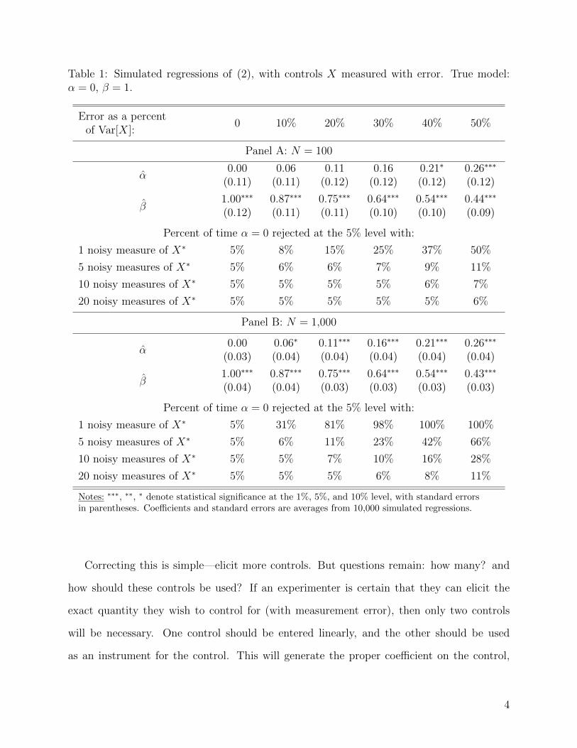
Table 1: Simulated regressions of (2), with controls X measured with error. True model:α = 0, β = 1.

Error as a percent0 10% 20% 30% 40% 50%

of Var[X]:

Panel A: N = 100

α0.00 0.06 0.11 0.16 0.21∗ 0.26∗∗∗

(0.11) (0.11) (0.12) (0.12) (0.12) (0.12)

β1.00∗∗∗ 0.87∗∗∗ 0.75∗∗∗ 0.64∗∗∗ 0.54∗∗∗ 0.44∗∗∗

(0.12) (0.11) (0.11) (0.10) (0.10) (0.09)

Percent of time α = 0 rejected at the 5% level with:

1 noisy measure of X∗ 5% 8% 15% 25% 37% 50%

5 noisy measures of X∗ 5% 6% 6% 7% 9% 11%



Panel B: N = 1,000

α0.00 0.06∗ 0.11∗∗∗ 0.16∗∗∗ 0.21∗∗∗ 0.26∗∗∗

(0.03) (0.04) (0.04) (0.04) (0.04) (0.04)

β1.00∗∗∗ 0.87∗∗∗ 0.75∗∗∗ 0.64∗∗∗ 0.54∗∗∗ 0.43∗∗∗

(0.04) (0.04) (0.03) (0.03) (0.03) (0.03)

Percent of time α = 0 rejected at the 5% level with:

1 noisy measure of X∗ 5% 31% 81% 98% 100% 100%




Notes: ∗∗∗, ∗∗, ∗ denote statistical significance at the 1%, 5%, and 10% level, with standard errorsin parentheses. Coefficients and standard errors are averages from 10,000 simulated regressions.

Correcting this is simple—elicit more controls. But questions remain: how many? and

how should these controls be used? If an experimenter is certain that they can elicit the

exact quantity they wish to control for (with measurement error), then only two controls

will be necessary. One control should be entered linearly, and the other should be used

as an instrument for the control. This will generate the proper coefficient on the control,

4

and thus, on the variable of interest D. However, it is doubtful that this will ever be the

case in practice. Even for a simple control like risk aversion, there are multiple, imperfectly

correlated, elicitation methods, as we discuss in Section 4. To ensure one is truly controlling

for all aspects of risk aversion, these need to be included in some form. However, including

multiple controls for multiple measures of multiple behaviors may entail the loss of too many

degrees of freedom to be practical.

Thus, in Section 3, we explore several different ways of including controls. First, we

include them linearly, as suggested by Table 1. Then, we show that principal component

analysis allows fro a small, but informative, set of controls—preserving degrees of freedom.

Finally, we elicit each control twice, and use the duplicate observation as an instrument.

These different approaches all lead to the same conclusion—the gender gap in competitiveness

can be explained by risk attitudes and overconfidence, although Niederle and Vesterlund

(2007) concluded that it was a disjoint phenomenon.

An attractive alternative to these approaches is to use specially designed controls. That

is, elicit behaviors that are designed to capture exactly the aspects of, say, risk aversion

that would influence the main task (van Veldhuizen, 2016). Indeed, Niederle and Vesterlund

(2007) follow exactly this approach by including a cleverly designed control meant to capture

risk-aversion and overconfidence in their environment. However, one must still be careful

with the statistical use of these controls. In particular, in the case of Niederle and Vesterlund

(2007), the control exhibits the issue shown in Table 1: the coefficient on it is too small.

A modification of their analysis that accounts for noise in the control brings their result

in line with ours. That is, in both their data and ours, there is no statistically significant

relationship between gender and competitiveness once risk-aversion and overconfidence are

properly accounted for.

The problem of measurement error biasing coefficients is particularly acute when re-

searchers estimate correlations between X and Y , as shown in the simulated results in Table

2. In this table, we simultaneously vary the proportion of measurement error in both vari-

5

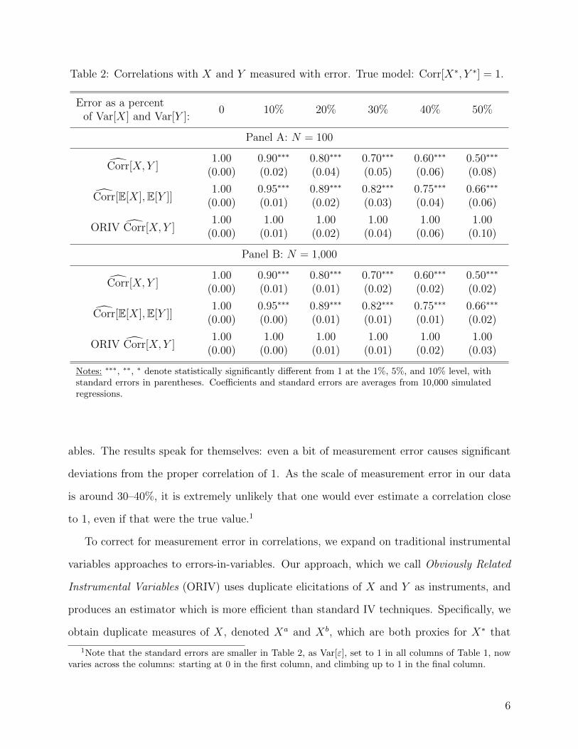
Table 2: Correlations with X and Y measured with error. True model: Corr[X∗, Y ∗] = 1.

Error as a percent0 10% 20% 30% 40% 50%

of Var[X] and Var[Y ]:

Panel A: N = 100

Corr[X, Y ]1.00 0.90∗∗∗ 0.80∗∗∗ 0.70∗∗∗ 0.60∗∗∗ 0.50∗∗∗

(0.00) (0.02) (0.04) (0.05) (0.06) (0.08)

Corr[E[X],E[Y ]]1.00 0.95∗∗∗ 0.89∗∗∗ 0.82∗∗∗ 0.75∗∗∗ 0.66∗∗∗

(0.00) (0.01) (0.02) (0.03) (0.04) (0.06)

ORIV Corr[X, Y ]1.00 1.00 1.00 1.00 1.00 1.00

(0.00) (0.01) (0.02) (0.04) (0.06) (0.10)

Panel B: N = 1,000

Corr[X, Y ]1.00 0.90∗∗∗ 0.80∗∗∗ 0.70∗∗∗ 0.60∗∗∗ 0.50∗∗∗

(0.00) (0.01) (0.01) (0.02) (0.02) (0.02)

Corr[E[X],E[Y ]]1.00 0.95∗∗∗ 0.89∗∗∗ 0.82∗∗∗ 0.75∗∗∗ 0.66∗∗∗

(0.00) (0.00) (0.01) (0.01) (0.01) (0.02)

ORIV Corr[X, Y ]1.00 1.00 1.00 1.00 1.00 1.00

(0.00) (0.00) (0.01) (0.01) (0.02) (0.03)

Notes: ∗∗∗, ∗∗, ∗ denote statistically significantly different from 1 at the 1%, 5%, and 10% level, withstandard errors in parentheses. Coefficients and standard errors are averages from 10,000 simulatedregressions.

ables. The results speak for themselves: even a bit of measurement error causes significant

deviations from the proper correlation of 1. As the scale of measurement error in our data

is around 30–40%, it is extremely unlikely that one would ever estimate a correlation close

to 1, even if that were the true value.1

To correct for measurement error in correlations, we expand on traditional instrumental

variables approaches to errors-in-variables. Our approach, which we call Obviously Related

Instrumental Variables (ORIV) uses duplicate elicitations of X and Y as instruments, and

produces an estimator which is more efficient than standard IV techniques. Specifically, we

obtain duplicate measures of X, denoted Xa and Xb, which are both proxies for X∗ that

1Note that the standard errors are smaller in Table 2, as Var[ε], set to 1 in all columns of Table 1, nowvaries across the columns: starting at 0 in the first column, and climbing up to 1 in the final column.

6

are measured with error. If measurement error in the two elicitations is orthogonal—as

we assume—then the predicted values Xa(Xb) from a regression of Xa on Xb contain only

information about X∗. We then use a stacked regression to combine the information from

both Xa(Xb) and Xb(Xa), resulting in an efficient use of the data.2 ORIV is easily extended

to allow for multiple measures of the outcome Y . This is particularly useful in estimating

correlations, where there is no clear distinction between outcome and explanatory variables,

and measurement error in either can attenuate estimates. ORIV is equivalent to using all

valid moment conditions in GMM, however it is simpler and more transparent. See Appendix

A for more on the relationship between ORIV and GMM.

ORIV produces consistent coefficients, correlations, and standard errors. This is in con-

trast to one common way experimenters deal with multiple and potentially noisy elicitations:

averaging the measures. As can be seen from Table 2, while averaging produces some reduc-

tion in inaccuracy, it still leads to incorrect conclusions in the presence of small amounts of

measurement error.

We apply ORIV, in Section 4, to show that various risk elicitation methods are more

correlated than previously thought, and that the patterns of correlations between them are

indicative of phenomena outside the lab. We further use this technique to show, in Section

5, that ambiguity aversion and reaction to compound lotteries are very close to perfectly

correlated—once we account for measurement error. This leads us to conclude, in Section

6, that failing to correct for measurement error has led the field to over-identify “new”

phenomena.

1.2 Related Literature

Mis-measurement of data has been an important concern for statisticians and econometri-

cians since the late 19th century (Adcock, 1878). Indeed, estimating the relationship between

2If measurement error is positively correlated across elicitations, then instrumented coefficients will stillbe biased downwards, although less so than without instrumenting. In our experimental design, we tried toweaken any possible correlation by varying the choice parameters, the grid of possible responses, and so on.See Section 2.1 and Section 4.4.2 for details and discussion.

7

two variables when both are measured with error is a foundational problem in the statistics

literature (Frisch, 1934; Koopmans, 1939; Wald, 1940). The use of instrumental variables

to address the classical errors-in-variables problem was proposed by Reiersøl (1941, 1945,

1950), with notable developments by Durbin (1954) and Sargan (1958) (see Hausman, 2001,

for a review). These techniques were first applied to economic problems by Friedman (1957),

who estimated consumption functions, and noted that annual income is a noisy measure of

permanent income, which would attenuate estimates of the marginal propensity to consume

from permanent income.3 Since then, instrumental variables have been used to account

for measurement error in an assortment of fields including medicine (Carroll and Stefanski,

1994), psychology (Fiske, Gilbert, and Lindzey, 2010), and epidemiology (Greenland, 2000).

The experimental literature has considered noise in lab data and its consequences, going

back to at least Kahneman (1965). Nonetheless, in the decade from 2006–2015 only 9% of the

283 experimental (field and lab) papers in Economics’ top 5 journals explicitly tried to deal

with measurement error. One-fifth of these papers either used an experimental design aimed

at reducing noise, or averaged multiple elicitations, a technique that may do little to reduce

bias, as shown in Section 1.1. About one-half of these papers estimate structural models

of participants’ “mistakes.” In particular, two-fifths estimate Quantal Response Equilibrium

models. Other than the few exceptions described below, most of the remaining papers use

indirect methods to deal with noise, such as the elimination of outliers, or the informal

derivation of additional hypotheses about the effects of noise, which are then tested.4

There are very few instances in which measurement error played an explicit role in the

analysis of experimental economics data. An early example, Battalio et al. (1973), shows

that even small reporting errors can lead to a rejection of the generalized axiom of revealed

preferences. In subsequent work, some scholars argued for a “theory of errors” under which

3For a review of the history and applications of instrumental variables more generally, see Angrist andKrueger (2001).

4We examined full, refereed papers published in The American Economic Review, Econometrica, Journalof Political Economy, The Quarterly Journal of Economics, and The Review of Economic Studies. A researchassistant found all experimental papers, then searched for a comprehensive list of keywords pertaining tomeasurement error.

8

observed violations of expected utility are an artifact of human error (Hey, 1991).5

Recent experimental papers have taken a renewed interest in the problems caused by mea-

surement error. Quantal Response Equilibrium posits a structural model in which agents

make mistakes that are inversely related to the payoff losses they generate (see McKelvey

and Palfrey, 1995, 1998; and applications described in Goeree, Holt, and Palfrey, 2016).

Using a related approach, Castillo, Jordan, and Petrie (2015), posit a structural model of

measurement error, following Harless and Camerer (1994). They use several risk elicitation

methods to study the effects of risk attitudes, accounting for measurement error, on disci-

plinary referrals of children. Coffman and Niehaus (2015) adjust for measurement error in

self-interest and other-regard by projecting both on a common set of explanatory variables.

Blattman et al. (2015), in a field setting, focus on gaining the trust of respondents in order

to quantify the amount of measurement error in responses to sensitive questions. 6 Our

paper is, to our knowledge, the first to offer simple, yet general, experimental techniques for

mitigating the effects of measurement error.7 Most of this work, like ours, consider classical

measurement error. However, by designing their experiments to produce more specific forms

of measurement error, experimenters may gain greater traction on their problem of interest.

Standard texts on the statistics of measurement error, such as Buonaccorsi (2010), provide

a wealth of opportunities.

Many of the issues measurement error raises for experimental work is present in survey

research as well. For example, (Bertrand and Mullainathan, 2001) describe the potential

5Drerup, Enke, and von Gaudecker (2016) do not correct for measurement error per-se, but rather observethat imprecise belief proxies may indicate behavioral rules that are less sensitive to beliefs. They test thishypothesis using data on stock market expectations and investment decisions.

6Recently, some experimental studies have included instrumental variables to deal with endogeneity (Fongand Luttmer, 2011; Hart and Middleton, 2014), and measurement error (Ambuehl and Li, 2015). Weizsacker(2010) considers errors in one explanatory variable in the context of social learning experiments. He treatsparticipants in the same experimental condition as replicants of each other, splits the sample of participantsin two, and uses one subset as an instrument for the other.

Dean and Ortoleva (2016) are the closest to the approach in our work. However, they estimate correlationsusing duplicates only on the right side, and without using them to properly estimate the variances of X∗

and Y ∗. Section 4 describes the issues with this approach.7List, Shaikh, and Xu (2016) also propose general techniques for dealing with a particular issue in exper-

iments, in their case multiple hypothesis testing in experimental work.

9

usefulness of surveys for economics and highlight the potential perils of measurement error.

(Bound, Brown, and Mathiowetz, 2001) also discuss potential biases due to measurement

error in survey research. Additionally, they review some of the contributions from social psy-

chology and survey methodology for identifying when measurement error may be important.

They advocate the collection of validation data to assess the importance of measurement er-

ror for results. They also note the potential usefulness of instrumental variable approaches.

The closest paper to ours in that literature is Beauchamp, Cesarini, and Johannesson (2015),

who consider measurement error in survey-based risk elicitations. They use a latent variable

model that allows them to make inferences about the component of measured risk attitudes

that is not due to measurement error. They emphasize, as we do, the ubiquity of measure-

ment error, and the paucity of concern about it.8

2 The Caltech Cohort Study

Caltech is an independent, privately supported university located in Pasadena, California.

It has around 900 undergraduate students, of which approximately 40% are women.

In the Fall of 2013, 2014, and Spring of 2015, we administered an incentivized, online

survey to the entire undergraduate student body. We used incentivized tasks to elicit an

array of attributes, including: risk aversion, ambiguity aversion, competitiveness, cognitive

sophistication, implicit attitudes toward gender and race, generosity, honesty, overconfidence,

overprecision, and optimism. Students were also asked a large set of questions addressing

their lifestyle and social habits: sleep patterns, study routines, social networks, study net-

works, physical attributes, and so on.9

The data used in this paper comes from the Fall 2014 and Spring 2015 installments. In

the Fall of 2014, 92% of the entire student body (893/972) responded to the survey. Of those,

8In a different context, Aguiar and Kashaev (2017) suggest a nonparametric statistical notion of ra-tionalizability of a random vector of prices and consumption streams when there is measurement error inconsumption levels reported in surveys. They use this test to assess standard exponential time discounting.

9For screenshots of the 2015 survey, go to: people.hss.caltech.edu/∼lyariv/ScreenshotsSpring2015.pdf.

10

http://people.hss.caltech.edu/~lyariv/papers/ScreenshotsSpring2015.pdf

39% were female (349/893), and the average payment was $24.34. In the Spring of 2015, 91%

of the entire student body (819/899) responded to the survey. Of those, 39% were female

(322/819), and the average payment was $29.08. The difference in average payments across

years was due to the inclusion of several additional incentivized items in 2015.10 Of those

who had taken the survey in 2015, 96% (786/819) also took the survey in 2014. As Section 4

requires data from both surveys, for consistency we use this subsample of 786 throughout.11

There are several advantages to using the CCS to address questions of measurement error.

The large size of the study allows us to document the non-existence of certain previously

identified “distinct” behaviors with unusual precision. Furthermore, the inflation of standard

errors that comes with using instrumental variables techniques does not threaten the validity

of our inferences. Last, unlike most experimental settings, there is little concern about self-

selection into our experiments from the participant population, due to our 90%+ response

rates (Cleave, Nikiforakis, and Slonim, 2013; Falk, Meier, and Zehnder, 2013; Harrison, Lau,

and Rutstrom, 2009). Thus, the issues we identify are due solely to measurement error, and

not due to a small sample or self-selection.

Nonetheless, Caltech is highly selective, which may cause one to worry that the overall

population is different from the pool used in most lab experiments. Three points should

mitigate this concern. First, the raw results of the replications are virtually identical to those

reported in the original papers.12 Second, responses from our survey to several standard

elicitations—of risk, altruism in the dictator game, etc.—are similar to those reported in

several other pools (see Appendix D for details). Third, while top-10 schools account for

0.32% of the college age population in the U.S., top-50 schools enroll only 3.77% of that

population (using the U.S. News and World Report rankings). Thus, there seems to be little

10The number of overall students was substantially lower in the Spring of 2015, as about 50 studentsdeparted the institute due to hardship or early graduation. Further, we did not approach students who hadspent more than four years at Caltech, accounting for approximately 25 students.

11In the Fall of 2013 88% of the student body (806/916) responded to the survey, of which 38.5% (310/806)were female. The average payment was $20.58. Of those who took the survey in 2013 and did not graduate,89% (546/615) also took the survey in the Fall of 2014.

12This should increase confidence in the original studies that we replicate, as it implies that it is notparticipants’ self-selection into the lab that is driving the results in those studies.

11

cause for concern that our participant pool is more “special” than that used in many other

lab experiments. As the results reported in this paper are replications of other studies, these

points suggest that our conclusions are likely due to our more sophisticated treatment of

measurement error, rather than an artifact of the participant population.

2.1 Measures Used

Our results deal with a subset of the measured attributes, which we detail here. Question

wordings can be found in Appendix E. Throughout, 100 survey tokens were valued at $1.

2.1.1 Overconfidence

We break overconfidence into three categories, following Moore and Healy (2008). These

measures are used in Section 3 as controls.

Overestimation and Overplacement: Participants complete two tasks: a five-question

cognitive reflection test (CRT; see Frederick, 2005), and five Raven’s matrices (Raven, 1936).

Participants are given a maximum of 20 seconds per CRT item, and 30 seconds per Raven’s

matrix. After each block of five questions, each participant is asked how many they think

they answered correctly. This, minus the participant’s true performance, gives a measure of

overestimation. Each participant is also asked where they think they are in the performance

distribution of all participants. This, minus the participant’s true percentile, gives a measure

of overplacement. This gives three co-linear measures: performance, expected performance,

and overconfidence; two of which can be used to control for confidence and overconfidence.

Overprecision: Participants are shown a random picture of a jar of jellybeans, and asked

to guess how many jellybeans the jar contains. They are then asked—on a six point quali-

tative scale from “Not confident at all” to “Certain”—how confident they are of their guess.

This is repeated three times. Following Ortoleva and Snowberg (2015), each of these mea-

sures is interpreted as a measure of overprecision.

12

Perception of Academic Performance: A final measure of overconfidence asks partic-

ipants to state where in the grade distribution of their entering cohort they believe they

would fall over the next year. This is treated as a measure of confidence in placement.

2.1.2 Risk

Risk measures are used in Section 3 as controls, and in Section 4 as an outcome of interest.

Further, the Risk MPL described below is used as an outcome of interest in Section 5.13

Projects: Following Gneezy and Potters (1997), participants are asked to allocate 200

tokens between a safe option (keeping them), and a project that returns some multiple of

the tokens with probability p, otherwise returning nothing. In Fall 2014, two projects were

used: the first returning 3 tokens per token invested where p = 40% of the time, and the

second returning 2.5 tokens 50% of the time. In the Spring of 2015, the first project was

modified to return 3 tokens 35% of the time.

Qualitative: Following Dohmen et al. (2011), participants are asked to rate themselves,

on a scale of 0–10, in terms of their willingness to take risks. As this question was only

asked once in the Fall of 2014, the elicitation from the Spring of 2015 is used as a duplicate

measure in Section 4.

Lottery Menu: Following Eckel and Grossman (2002), participants are asked to choose

between six 50/50 lotteries with different stakes.14 The first lottery contained the same

payoff in each state, and thus corresponded to a sure amount. The remaining lotteries

contain increasing means and variances, allowing for an estimation of risk aversion.

Risk MPL: Participants respond to two Multiple Price Lists (MPLs) that ask them to

choose between a lottery over a draw from an urn, and sure amounts. The lottery would pay

13For an overview of risk elicitation techniques, see Charness, Gneezy, and Imas (2013).14The variant we use comes from Dave et al. (2010).

13

off if a ball of the color of the participant’s choosing was drawn. The first urn contained 20

balls—10 black and 10 red—and paid 100 tokens. The second contained 30 balls—15 black

and 15 red—and paid 150 tokens. Taking the first MPL as an example, participants are first

asked to choose the color (red or black) that they want to pay off, if drawn. They are then

presented with a list of choices between a certainty equivalent that increases in units of 10

tokens from 0 to 100 or the gamble on the urn.15

2.1.3 Ambiguity and Compound Lotteries

Reactions to ambiguous and compound lotteries are considered in Section 5.

Compound MPL: This follows the same protocol as the Risk MPLs described above,

except participants are told that the number of red balls would be uniformly drawn between

0 and 20 for the first urn, and between 0 and 30 for the second. As this is a measure of risk

attitudes, it is also used as a control in Section 4.

Ambiguous MPL: This elicitation emulates the standard Ellsberg (1961) urn. It follows

the same protocol as the two other MPLs. Participants were informed that the composition

of the urn was chosen by the Dean of Undergraduate Students at Caltech.

To reduce instructions, both of the MPLs for a given attitude (Risk, Compound, Ambi-

guity) are run sequentially, in random order. These three blocks are spread across the survey,

and which block is given first, second, and third is randomly determined. As no order effects

were observed, we aggregate results across the different possible orderings.

15In order to prevent multiple crossovers, the online form automatically selected the lottery over a 0 tokencertainty equivalent, and 100 tokens over the lottery. Additionally, participants needed only to make onechoice and all other rows were automatically filled in to be consistent with that choice.

14

3 Mis-specified Controls and Measurement Error

To make the claim that an estimated effect is independent of other factors, many studies

attempt to control for those other factors. If those other factors are measured with error,

one control, or even a few, may be insufficient to reliably assert the claim, as illustrated in

Section 1.1. That section also showed that more controls can ameliorate this issue. Here we

illustrate that properly dealing with controls measured with error has important substantive

consequences. We do so by replicating the competitiveness and gender study of Niederle and

Vesterlund (2007)—henceforth NV—within the CCS. Like NV, we find a robust difference

in the rates at which men and women compete. However, NV conclude that:

Finally, controlling for gender differences in general factors such as overconfi-dence, risk, and feedback aversion, we estimate the size of the residual genderdifference in the tournament-entry decision. Including these controls, gender dif-ferences are still significant and large. Hence, we conclude that, in addition togender differences in overconfidence, a sizeable part of the gender difference intournament entry is explained by men and women having different preferencesfor performing in a competitive environment.

In contrast, we show that the gender gap is well explained by risk aversion and overconfidence.

Using the notation of Section 1.1, measurement error in X, in this case controls for risk

aversion and overconfidence, can result in a biased estimate of the coefficient on D, in this

case gender, on competition Y . To understand this intuitively, consider the model in (1)

where Y ∗ = X∗, D and X∗ are correlated, and X = X∗ + ν is a noisy measure of X∗. For

illustration, consider an extreme case where the variance of ν is very large, so that X is almost

entirely noise. If a researcher ignores that noise in X, standard regression analysis could then

lead to the erroneous conclusion that Y and D are correlated, even when controlling for X.16

To put this in terms of our substantive example, it is well known that overconfidence is

correlated with gender (see, for example, Moore and Healy, 2007, 2008), and, depending on

the elicitation method, risk aversion may be correlated with gender as well (see Holt and

16It is well known that measurement error in left-side variables may bias estimated coefficients in discretechoice models, see Hausman (2001). Thus, as Y may also be measured with error, we use linear probabilitymodels to avoid bias.

15

Laury, 2014, for a survey, and our discussion in Section 4.6). Thus, if competitiveness is

driven by overconfidence or risk aversion, mis-measurement of these traits will lead to an

overestimate of the effect of gender.

What can be done to mitigate this issue? The simplest approach, which we take, is

to include multiple measures for each of the possible controls X. This approach reduces

the effects of measurement error, while helping to ensure that elicited controls cover the

potentially different aspects of the behavioral attribute being controlled for.

3.1 Measuring Competitiveness in the Caltech Cohort Study

Part of the Spring 2015 survey mimicked the essential elements of NV’s design. Participants

first had three minutes to complete as many sums of five two-digit numbers as they could.

The participants were informed that they would be randomly grouped with three others at

the end of the survey. If they completed the most sums in that group of four, they would

receive 40 experimental tokens (or $0.40) for each sum correctly solved, and would otherwise

receive no payment for the task. Ties were broken randomly. As in NV, at the end of this

task, participants were asked to guess their rank, from 1 to 4, within the group of four

participants. They were paid 50 tokens (or $0.50) if their guess was correct.

Next, in the central task of NV’s design, participants were told they would have an

additional three minutes to complete sums. However, before doing so, they chose whether

to be paid according to a piece-rate scheme or a tournament. The piece-rate scheme paid

10 tokens for each correctly solved sum. The tournament had a similar payment scheme

to the first three-minute task. The difference was that the participant’s performance in the

tournament would be compared to the performance of three randomly chosen participants

in the first task. This ensured that the participant would not need to be concerned about

the motivation, or other characteristics, that might drive someone to compete in the second

task. Otherwise, the payment structure was identical to that in the first task.

There are a few ways in which our implementation differs from NV’s:

16

Time and Payments: We gave participants three, rather than five, minutes to complete

sums. Per-sum payments were scaled down by a factor of four. As with the rest of the

CCS, participants were paid for all tasks, rather than a randomly selected one. This

could have caused participants to hedge by choosing the piece-rate scheme.

Grouping of Participants: In NV, participants were assigned to groups of four where they

could visibly see that there were two men and two women. This created an imbalance

in the expected number of female competitors: for men this was 2/3 of the group,

versus 1/3 for women. In the CCS, we randomly selected groups after the survey was

administered, and created different groups for the first and second task. Thus, both

genders faced the same expected profile of competitors.

Experimental Setting: Our elicitation was done on a survey, whereas NV used a lab

setting. Administering our survey several months later in a lab environment to 98

Caltech students produced very similar results, but with larger standard errors driven

by the smaller sample.

Additional Tasks: NV include two additional parts: a preliminary task allowing partici-

pants to try out the piece-rate scheme, and a final choice that allows participants to

select either an additional piece-rate or tournament payment scheme for their perfor-

mance in the preliminary task. This final choice served as a control for risk aversion

and overconfidence. As the CCS has multiple other controls for both of these traits

(see Section 2.1), we omitted these two parts to reduce the complexity and time taken

to elicit competitiveness.

The first three of these factors would only change interpretation if they affected men and

women differently. However, as we replicate the gender gap in tournament entry found by

NV, these do not seem to be of particular importance. The final factor implies that we cannot

use an analogous control to that of NV’s with the CCS data. Nonetheless, using NV’s data

and an analysis accounting for measurement error in their control, we find that the gender

17

gap in tournament entry can be explained by risk aversion and overconfidence (see Section

3.3). More details about our, and NV’s, implementation can be found in Appendix E.1.

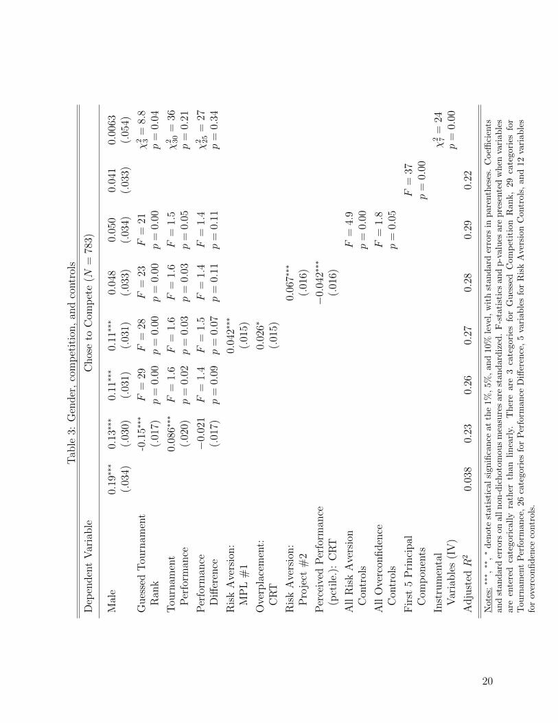
3.2 Gender, Competition, and Controls

This subsection analyzes the extent to which risk aversion and overconfidence drive the

gender gap in competitiveness. Table 3 summarizes specifications meant to illustrate different

points. These are linear probability models, and hence, the coefficient on gender is directly

interpretable as the percentage-point gap between men and women in choosing to compete.17

The first column shows the baseline difference in competition: Women choose tournament

incentives 21.4% of the time, while men choose them 40.4% of the time, for a difference of 19.0

percentage points. This difference is highly statistically significant. While these numbers are

somewhat lower than those reported in NV, their relative sizes are quite similar. The second

column controls for participants’ estimates of their own rank, as well as their performance,

linearly, as in NV’s main specification. Similar to their results, the inclusion of these controls

reduces the coefficient on gender by approximately 1/3.

There is, however, a non-linear relationship between expected rank and perceived prob-

ability of victory in a competition.18 Therefore, the third column enters participants’ sub-

jective ranks non-parametrically, by including a dummy variable for each possible response

(three categories). This estimation confirms that the effect of perceived rank in a compe-

tition is, indeed, non-linear, although the coefficient on gender remains unchanged.19 The

third column also enters performance non-linearly (29 and 26 categories, respectively), as

17As noted in Footnote 16, discrete choice models may produce biased estimates of coefficients when theleft-side variable is measured with error. Nonetheless, in our data, Probit and Logit specifications producealmost identical levels of statistical significance as in Table 3.

18If an individual believes a random participant is inferior to her with probability p, then her probabilityof winning is p3. Furthermore, her expected rank is given by

∑3i=0(i + 1)

(3i

)(1− p)i p3−i = 3(1 − p) + 1.

We can therefore back out the probability p from any reported rank r (ignoring rounding). With a reported

rank of r, the probability of winning the competition is(4−r3

)3.

19Rates of competition are 65.6% for participants who predicted they would come in first (in a randomgroup of 4), and 31.4%, 15.3%, and 5.0% for participants predicting they would come in second, third,and fourth (last), respectively. The distribution of guessed ranks differs from that reported in NV: ourparticipants were better calibrated, and this likely resulted in the lower observed rates of tournament entry.

18

there is also a non-linear relationship between performance and competition. The coefficient

on gender in the third column is lower than in the second.20

The fourth column begins introducing additional controls for risk aversion and overcon-

fidence. In this column, two (non-randomly) selected controls are entered, one for each

attribute. As can be seen, this does not affect the coefficient on gender, despite the fact

that both controls have statistically significant coefficients. The fifth column contains a

different two (non-randomly) selected controls; this cuts the coefficient on gender by more

than half, and renders it statistically insignificant. Taken together, these columns show that

the statistical significance of controls is not a good indicator of whether or not a trait is

fully controlled for. Moreover, it suggests that measurement error in the controls themselves

allows for the perception of competitiveness as a separate trait.

It is worth noting that these conclusions are not driven by our unusually large sample size.

If anything, the size of our dataset helps reduce standard errors and identify weak effects

that, with a smaller dataset, would appear insignificant. To see this, we draw a random

sample of 40 women and 40 men (the size and gender composition of NV’s experiment) from

our data 10,000 times, and regress the competition decision on two overconfidence controls,

two risk controls, and perceived rank in the first competition task. The coefficient on gender

is significant at the 1% level 2.2% of the time, at the 5% level 7.6% of the time, and at the

10% level 13% of the time.

The sixth column enters all available controls for risk (6 controls) and overconfidence (an

additional 12 controls). The coefficient on gender is relatively unchanged, which masks the

fact that additional controls first cause the coefficient to fall, and then rise, although never

by much. If we enter these controls separately, we find that much of the decrease in this

coefficient, as compared to the third column, is due to the controls for risk aversion. We

revisit the relationship between gender and risk aversion in Section 4.6.

20This is entirely driven by including performance in the first task non-parametrically, as there are smalldifferences in male and female performance in this task, as shown in Figure E.2 of Appendix E.1.

19

Tab

le3:

Gen

der

,co

mp

etit

ion,

and

contr

ols

Dep

enden

tV

aria

ble

Chos

eto

Com

pet

e(N

=78

3)

Mal

e0.

19∗∗∗

0.13∗∗∗

0.11∗∗∗

0.11∗∗∗

0.04

80.

050

0.04

10.

0063

(.03

4)(.

030)

(.03

1)(.

031)

(.03

3)(.

034)

(.03

3)(.

054)

Gues

sed

Tou

rnam

ent

-0.1

5∗∗∗

F=

29F

=28

F=

23F

=21

χ2 3

=8.

8R

ank

(.01

7)p

=0.

00p

=0.

00p

=0.

00p

=0.

00p

=0.

04

Tou

rnam

ent

0.08

6∗∗∗

F=

1.6

F=

1.6

F=

1.6

F=

1.5

χ2 30

=36

Per

form

ance

(.02

0)p

=0.

02p

=0.

03p

=0.

03p

=0.

05p

=0.

21

Per

form

ance

−0.

021

F=

1.4

F=

1.5

F=

1.4

F=

1.4

χ2 25

=27

Diff

eren

ce(.

017)

p=

0.09

p=

0.07

p=

0.11

p=

0.11

p=

0.34

Ris

kA

vers

ion:

0.04

2∗∗∗

MP

L#

1(.

015)

Ove

rpla

cem

ent:

0.02

6∗

CR

T(.

015)

Ris

kA

vers

ion:

0.06

7∗∗∗

Pro

ject

#2

(.01

6)

Per

ceiv

edP

erfo

rman

ce−

0.04

2∗∗∗

(pct

ile.

):C

RT

(.01

6)

All

Ris

kA

vers

ion

F=

4.9

Con

trol

sp

=0.

00

All

Ove

rcon

fiden

ceF

=1.

8C

ontr

ols

p=

0.05

Fir

st5

Pri

nci

pal

F=

37C

omp

onen

tsp

=0.

00

Inst

rum

enta

lχ

2 7=

24V

aria

ble

s(I

V)

p=

0.00

Adju

sted

R2

0.03

80.

230.

260.

270.

280.

290.

22

Not

es:∗∗∗ ,∗∗

,∗

den

ote

stat

isti

cal

sign

ifica

nce

at

the

1%

,5%

,an

d10%

leve

l,w

ith

stan

dard

erro

rsin

pare

nth

eses

.C

oeffi

cien

tsan

dst

and

ard

erro

rson

alln

on-d

ich

otom

ou

sm

easu

res

are

stan

dard

ized

.F

-sta

tist

ics

an

dp-v

alu

esare

pre

sente

dw

hen

vari

ab

les

are

ente

red

cate

gori

call

yra

ther

than

lin

earl

y.T

her

eare

3ca

tegori

esfo

rG

ues

sed

Com

pet

itio

nR

ank,

29

cate

gori

esfo

rT

ourn

amen

tP

erfo

rman

ce,

26ca

tego

ries

for

Per

form

an

ceD

iffer

ence

,5

vari

ab

les

for

Ris

kA

vers

ion

Con

trols

,an

d12

vari

ab

les

for

over

con

fid

ence

contr

ols.

20

The number of controls in the sixth column (76, including categorical controls for perfor-

mance) approaches the number of data points in a normally sized study—such as NV, which

had 80 participants. Thus, we examine ways to preserve degrees of freedom. The simplest is

to perform a principal components analysis of all 76 of the controls. The first few principal

components will contain most of the information in those controls—in this case entering just

5 of them produces a very similar point estimate to entering all 76 controls. More on this

technique can be found in Appendix B.1.

As discussed in Section 1.1, the potential bias in the coefficient on gender comes from

the fact that the coefficients on the noisy controls—assumed to be positively correlated with

both gender and competitive behavior—are biased towards zero. Thus, in the final column,

we instrument the risk aversion and overconfidence controls for which we have multiple

elicitations. This approach combines consistent estimates of the coefficients on controls, while

still ensuring that we span the space of possible aspects of risk aversion and overconfidence in

our data. While the point estimate of the coefficient on gender is consistent (and statistically

insignificant), it is also accompanied by the higher standard errors that come with an IV

specification. We exploit these multiple elicitations and IV strategies, more fully in Sections

4 and 5. However, we first turn to another avenue for achieving the correct coefficient on

controls that can be applied to those designed with a specific purpose in mind.

3.3 Using Designed Controls

NV control for risk aversion and overconfidence with another tournament entry choice.

Namely, in the last stage of their experiment, participants are given a second opportunity

to be paid for their performance in the piece-rate task from the beginning of the experi-

ment. They can choose to be paid again as a piece rate, or to enter their performance into a

tournament. The clever idea behind this additional choice is that it controls for all aspects

determining tournament entry that are not directly related to a preference for competing—

explicitly, risk aversion and overconfidence. We show that a specification that accounts for

21

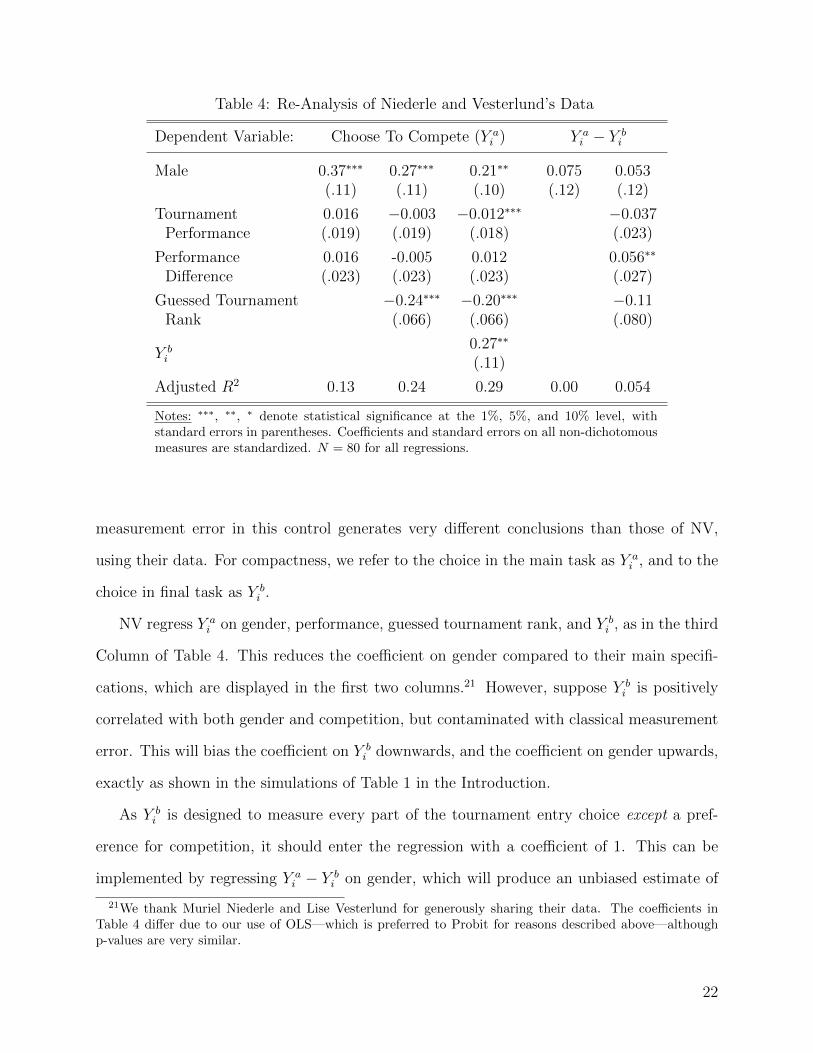
Table 4: Re-Analysis of Niederle and Vesterlund’s Data

Dependent Variable: Choose To Compete (Y ai ) Y a

i − Y bi

Male 0.37∗∗∗ 0.27∗∗∗ 0.21∗∗ 0.075 0.053(.11) (.11) (.10) (.12) (.12)

Tournament 0.016 −0.003 −0.012∗∗∗ −0.037Performance (.019) (.019) (.018) (.023)

Performance 0.016 -0.005 0.012 0.056∗∗

Difference (.023) (.023) (.023) (.027)

Guessed Tournament −0.24∗∗∗ −0.20∗∗∗ −0.11Rank (.066) (.066) (.080)

Y bi

0.27∗∗

(.11)

Adjusted R2 0.13 0.24 0.29 0.00 0.054

Notes: ∗∗∗, ∗∗, ∗ denote statistical significance at the 1%, 5%, and 10% level, withstandard errors in parentheses. Coefficients and standard errors on all non-dichotomousmeasures are standardized. N = 80 for all regressions.

measurement error in this control generates very different conclusions than those of NV,

using their data. For compactness, we refer to the choice in the main task as Y ai , and to the

choice in final task as Y bi .

NV regress Y ai on gender, performance, guessed tournament rank, and Y b

i , as in the third

Column of Table 4. This reduces the coefficient on gender compared to their main specifi-

cations, which are displayed in the first two columns.21 However, suppose Y bi is positively

correlated with both gender and competition, but contaminated with classical measurement

error. This will bias the coefficient on Y bi downwards, and the coefficient on gender upwards,

exactly as shown in the simulations of Table 1 in the Introduction.

As Y bi is designed to measure every part of the tournament entry choice except a pref-

erence for competition, it should enter the regression with a coefficient of 1. This can be

implemented by regressing Y ai − Y b

i on gender, which will produce an unbiased estimate of

21We thank Muriel Niederle and Lise Vesterlund for generously sharing their data. The coefficients inTable 4 differ due to our use of OLS—which is preferred to Probit for reasons described above—althoughp-values are very similar.

22

the effect of gender on tournament entry, controlling for Y bi . Intuitively, the only difference

between these two variables is, by construction, a desire to compete. To see if this desire

is correlated with gender, it should be regressed on gender. Doing so results in an insignif-

icant coefficient on gender of 0.075. The inclusion of additional controls on the right side

reduces the coefficient even further.22 Thus, had NV used a specification that accounts for

measurement error in Y bi , they would have come to the same conclusion: risk aversion and

overconfidence explain the gender gap in tournament entry.

3.4 Substantive Interpretation

Our analysis shows, using both new data, and data from NV, that although men are more

likely to select into competition, this is not due to a distinct preference for performing in a

competitive environment. Rather, it is driven by differences in risk aversion and overconfi-

dence. It is important to note that using multiple controls for risk aversion and overconfi-

dence, or using principal components, does not allow us to say how important either of these

factors is in explaining competition, only that together they explain much of the effect.23

Our results do not, by any means, imply that it is better to elicit risk attitudes and over-

confidence instead of competitiveness. There is a tradeoff: competition is potentially more

directly relevant for an array of economically important decisions, and is definitely a more

parsimonious measure. Indeed, competition has been shown to explain several interesting

behaviors, such as choice of college major (see, for example, Buser, Niederle, and Oosterbeek,

2014). However, risk aversion and overconfidence feature in many theories, and are therefore

of potential use in bringing theory to bear on gender differences.

There are also practical considerations. NV report that their experiment had an average

runtime of approximately 45 minutes. By using two tasks (rather than four) and allowing

22The inclusion of additional controls should make the test more efficient in small samples, see AppendixB.2 for a formal exposition of this, and other points, in this sub-section.

23Recent work by van Veldhuizen (2016) uses clever experimental design to add refined versions of NV’sfinal task, and specifications following the previous subsection, to estimate the effect of risk-aversion, over-confidence, and a taste for competition on tournament entry. He arrives at a similar conclusion to ours: thegender gap in tournament entry is entirely driven by differences in risk aversion and overconfidence.

23

participants to solve sums for three minutes (rather than five), we reduced the average time

participants spent on the competition task to around 8 minutes. Naturally, eliciting multiple

measures of risk and overconfidence may be time consuming as well. Nevertheless, our entire

survey had an average runtime of less than 30 minutes, including the competition task.

4 Measurement Error Left and Right

We now shift to a situation where the variables of interest, rather than controls, are measured

with error. This attenuates the estimated relationship between different variables. We

introduce a simple method, Obviously Related Instrumental Variables (ORIV)—which is

more efficient than standard IV techniques—to correct for this.24 We apply this technique

to the estimation of the correlation between different measures of risk attitudes in this section,

and between risk and ambiguity aversion in the next.

It is well known that measurement error in outcome, or dependent, variables does not

bias estimated relationships, although it increases standard errors. Measurement error in

explanatory, or dependent, variables is a much more serious problem, biasing estimated

coefficients and distorting standard errors. This leads to an improper understanding of the

relationship between explanatory variables and outcomes. These problems are compounded

when estimating a correlation: the distinction between outcome and explanatory variables

is blurred, and classical measurement error in either biases estimates towards zero.

The following subsections develop the ORIV approach gradually. The first subsection

introduces the substantive question of investigating correlations between different risk mea-

sures. The next gives a simple treatment of the standard application of instrumental variables

to correct for measurement error in explanatory variables. The following three subsections

show, theoretically and empirically, how to combine information from multiple instruments,

and how to consistently estimate correlation coefficients when both explanatory and outcome

24How much more efficient depends on the number of replicated observations. For the standard case wherethere are two elicitations of both variables, the ORIV estimator is twice as efficient—that is, the variance ofthe ORIV estimator is one-half that of IV estimates.

24

variables are measured with error. The discussion in this section focuses on implementation,

with the formal properties of the estimators developed in Appendix A.

4.1 Risk Elicitation Techniques

There is a substantial experimental literature assessing the validity of common experimental

techniques for eliciting attitudes towards risk and uncertainty (see the literature review in

Holt and Laury, 2014). These studies often elicit risk attitudes in the same set of participants

using different techniques. By using a within-participant design, researchers attempt to

understand technique-driven differences in elicited proxies for risk aversion. This type of

work has generally found small correlations between different techniques, making it difficult

to study the individual correlates of risk preferences. To mention a few examples, Dave

et al. (2010) compare the Lottery Menu task with the Holt and Laury (2002) task—in which

participants choose one lottery in each of a sequence of lottery pairs, where means and

variances change from pair to pair. Participants appear to be more risk averse in the Holt

and Laury task. Deck et al. (2008) compare behavior in the Holt and Laury task to that in

a task that was a variation on the game show “Deal or No Deal,” and report a correlation

between risk attitudes from the two tasks at only 0.008, with a p-value of 0.94. Deck et al.

(2010) compare the same two tasks, adding two others (including the Lottery Menu task

used here), as well as survey questions touching upon risk in six different domains. The

highest pairwise correlations they find are lower than 0.3. Similarly, Anderson and Mellor

(2009) compare responses to the Holt and Laury task to survey questions about hypothetical

gambles. They find small correlations, and provide a survey of the literature with similar

results. Loomes and Pogrebna (2014) compare three different risk elicitations: the Risk MPL

and Lottery Menu elicitations we use, as well as risky allocation task borrowed from Loomes

(1991), which resembles our Projects task. They find significant variability both within and

between elicitations.

Ultimately, the literature concludes that risk elicitation is a “risky business”—the pun is

25

not ours, see Friedman et al. (2014) for a survey. Indeed, those authors conclude that:

Estimated parameters exhibit remarkably little stability outside the context inwhich they are fitted. Their power to predict out-of-sample is in the poor-to-nonexistent range, and we have seen no convincing victories over naive alterna-tives.

However, none of the studies on which this conclusion is based account for measurement error

when estimating correlations between elicitation techniques. In what follows, we inspect sev-

eral commonly used risk-attitude elicitation techniques, and estimate their within-participant

correlations using an IV strategy to account for measurement error. This generates much

higher within-participant correlations than previously reported. Moreover, the corrected

correlations suggest that elicitation techniques fall into one of two sets: those that elicit

certainty equivalents for lotteries, and those that elicit allocations of assets between safe and

risky options. The latter category exhibits greater corrected correlations with other mea-

sures, and more stability over time. Further, elicitations based on allocation decisions display

substantial gender effects—which are consistent with investment behavior in the field—while

certainty equivalent elicitations do not.

This section uses four measures of risk as described in Section 2.1: Qualitative, Risk MPL,

Project, and Lottery Menu. Before we proceed, we note a few details about how we handle

the data from those elicitations to standardize estimated quantities for easy comparison.

First, when using two measures from the same form of elicitation, we put these on a common

scale. In particular, the certainty equivalents from the 30-ball urn Risk MPL (which go up

to 150) are divided by 1.5 to be on the same scale as the certainty equivalents from the 20-

ball urn Risk MPL (which go up to 100).25 Second, when comparing objects like estimated

CRRA coefficients or derived certainty equivalents, these are also put on the same scale.

For example, when examining the relationship between certainty equivalents from the Risk

MPLs and Projects—the former allowing for risk-loving answers and the latter not—those

who gave risk-loving answers on the urns are re-coded to give a risk-neutral answer. Without

25This implicitly assumes a CRRA utility function.

26

this censoring, results are qualitatively similar.26

4.2 A First Take on Measurement Error Correction

It is well known that measurement error attenuates estimated coefficients (see, for example,

Greene, 2011). Here we review that basic finding to set up a framework for our estimator.

To estimate the relationship between two variables measured with independent i.i.d. error,

Y = Y ∗ + νY and X = X∗ + νX (with E[νY νX ] = 0 and Var[νk] = σ2νk

), the ideal regression

model would be Y ∗ = α∗+β∗X∗+ ε∗. Instead, we can only estimate Y = α+βX+ ε, where

α is a constant and ε is a mean-zero random noise. Annotating finite-sample estimates with

hats and population moments without hats, this results in an estimated relationship of

β =Cov[Y,X]

Var[X]=

Cov[α + β∗X∗ + ε+ νY , X∗ + νX ]

Var[X∗ + νX ]

E[β]

= plimn→∞

β = β∗σ2X∗

σ2X∗ + σ2

νX

< β∗. (3)

The estimated coefficient β is thus biased towards zero. Importantly, the bias in (3) depends

on the amount of information about the true explanatory variable X∗ in X.

In a lab experiment, it is relatively easy to elicit two replicated measures of the same

underlying parameter X∗. That is, suppose we have Xa = X∗ + νaX and Xb = X∗ + νbX ,

with νaX , νbX i.i.d. random variables, and E

[νaXν

bX

]= 0—that is, measurement errors are

independent of each other, and thus uncorrelated. With the additional assumption that

Var[νaX ]

Var[Xa]=

Var[νbX ]

Var[Xb]≡ Var[νX ]

Var[Xa], we have

Corr[Xa, Xb]→p Corr[Xa, Xb] =σ2X∗

σ2X∗ + σ2

νX

, (4)

which allows us to ballpark the degree of bias in estimated coefficients. The modal correlation

between two elicitations of the same risk measure is approximately 0.6, suggesting that the

26This censoring affects 22% of the responses in the 20-ball urn, and 32% of responses in the 30-ball urn.

27

variance of measurement error is of the order of 2/3 of the variance of X∗.27

Using instrumental variables (IV), the second noisy measure of X∗ can be used to recover

a consistent estimate of the true coefficient β∗. Recalling from the derivation of (3) that

Cov[Xa, Xb] = Var[X∗], we use two-stage-least-squares (2SLS) to instrument Xa with Xb

Xa = π0 + π1Xb + εX ⇒ π1 =

Cov[Xa, Xb]

Var[Xb]=

Var[X∗]

Var[Xb], (5)

and then condition on this instrumented relationship to estimate Y = α+β(π0 + π1Xb)+εY .

This second stage regression provides

β =Cov[α∗ + β∗X∗ + ε∗ + νY , π0 + π1X

b]

Var[π0 + π1Xb]=β∗π1Var[X∗]

π21Var[Xb]

→p β∗,

a consistent estimate of β∗, the true relationship between Y ∗ and X∗.

4.3 Two Instrumentation Strategies

Multiple measures for X∗ admit multiple instrumentation strategies that will only produce

the same estimate with infinite data. The ORIV estimator consolidates the information from

these different formulations of the problem to provide an estimator that is twice as efficient

as either IV strategy alone. That is, the variance of the ORIV estimator is half that of either

IV estimator. Combining these estimators is the same as using both valid moment conditions

in GMM, see Appendix A. ORIV offers a simpler and more transparent correction technique

than GMM. In the settings we consider, it is equally efficient. In our working example,

27In practice, if one is certain that the variation in Xa and Xb due to X∗ is the same, then one can measurethe proportion of measurement error in each elicitation j separately as Cov[Xa, Xb]/Var[Xj ]. However,lacking that certainty, it is advisable to standardize variables, at which point the formulation here and in(4) coincide.

This correlation also provides a way to derive a correction factor for the attenuation bias in the regressionestimates from (3) dating back to Spearman (1904). Defining the “disattenuated” estimator of β as β =

β

Corr[Xa,Xb]and invoking the continuous mapping theorem, it is clear that β provides a consistent estimator

for β. This approach, while consistent, may be inefficient in the presence of multiple replicates. As illustratedin Appendix A, the ORIV approach provides a simple formulation for consolidating the information frommultiple replicates of both X and Y .

28

Tab

le5:

Cor

rela

tion

bet

wee

ndiff

eren

tri

skm

easu

res

isunder

stat

eddue

tom

easu

rem

ent

erro

r.

Dep

enden

tV

aria

ble

Qual

itat

ive

Ass

essm

ent

Lot

tery

Men

u

Pro

ject

#1

0.30∗∗∗

0.24∗∗∗

(.03

4)(.

034)

Pro

ject

#2

0.29∗∗∗

0.29∗∗∗

(.03

4)(.

034)

Pro

ject

#1

0.55∗∗∗

0.60∗∗∗

(Inst

rum

ente

d)

(.06

7)(.

073)

Pro

ject

#2

0.58∗∗∗

0.50∗∗∗

(Inst

rum

ente

d)

(.06

9)(.

070)

Ris

kM

PL

#1

0.16∗∗∗

0.19∗∗∗

(.03

6)(.

035)

Ris

kM

PL

#2

0.17∗∗∗

0.23∗∗∗

(.03

5)(.

035)

Ris

kM

PL

#1

0.22∗∗∗

0.44∗∗∗

(Inst

rum

ente

d)

(.04

8)(.

069)

Ris

kM

PL

#2

0.21∗∗∗

0.37∗∗∗

(Inst

rum

ente

d)

(.04

7)(.

067)

Not

es:∗∗∗ ,∗∗

,∗

den

ote

stat

isti

cal

sign

ifica

nce

at

the

1%

,5%

,an

d10%

leve

l,w

ith

stand

ard

erro

rsin

pare

nth

eses

.C

oeffi

cien

tsar

efr

omre

gres

sion

sw

her

eb

oth

the

right

an

dle

ft-s

ide

vari

ab

les

are

stan

dard

ized

,an

dth

us

are

corr

elati

on

s.N

=77

5.

29

we have two equally valid elicitations and two possible instrumentation strategies: one may

instrument Xa with Xb, or Xb with Xa. In this subsection, we illustrate the divergent results

these two strategies may produce. The next subsections show how to deal with this issue by

combining these sources of information into a single estimated relationship.

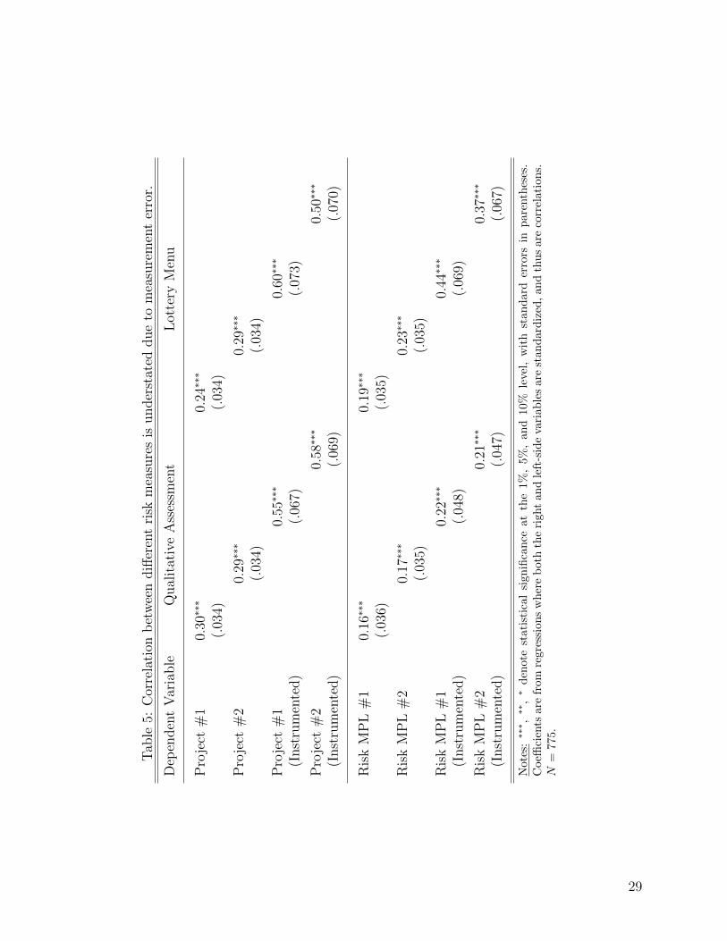
Table 5 shows estimated relationships between different elicitation techniques. These are

first estimated using a standard regression, and then the two different IV strategies discussed

above. The coefficients are from regressions where both the left- and right-side variables are

standardized, which removes scale effects and provides for easy comparison.

Although different instrumentation strategies may produce similar results—as in the third

and fourth columns of Table 5—they can also produce different results—as in the seventh

and eighth columns. Moreover, given that estimated standard deviations, which are inflated

by measurement error, are used to standardize the variables in Table 5, neither strategy is

likely to produce an accurate result. The next subsection deals with both of these issues.

4.4 Obviously Related Instrumental Variables

We construct ORIV estimates and corrected correlations in three steps. First, we consider the

case where only explanatory variables are measured with error. We then extend the analysis

to the case where both the outcome and explanatory variables are measured with error.

Finally, we show how to derive consistent correlations from the consistent and asymptotically

efficient ORIV estimates of the regression coefficient β. Throughout, we focus on designs in

which there are at most two replications for each measure. This is done for simplicity, and

because it fits precisely the implementation carried out using the Caltech Cohort Study.28

4.4.1 Errors in Explanatory Variables

We continue with the model stated in Section 4.2, noting that unlike the analysis in Section

4.3, these measures are not standardized. The ORIV regression estimates a stacked model

28Appendix A extends the ORIV estimator to settings where more than one replicate is available.

30

to consolidate the information from the two available instrumentation strategies:

(Y

Y

)=

(α1

α2

)+ β

(Xa

Xb

)+ ε, instrumenting

(Xa

Xb

)with W =

Xb 0N

0N Xa

, (6)

where N is the number of participants, and 0N is an N ×N matrix of zeroes. To implement

this, one need only to create a stacked dataset and run a 2SLS regression. This can be

thought of as estimating a first stage, as in (5), for both instrumentation strategies, and

then estimating (Y

Y

)=

(α1

α2

)+ β

(Xa

Xb

)+ ε, (7)

where Xa and Xb are the predicted values derived from the two first-stage regressions.

Sample Stata code illustrating this estimation procedure appears in Appendix C.2.29

With a single replication, the stacked regression will produce an estimate of β∗ that is

the average of the estimates from the two instrumentation approaches in prior subsections.

Intuitively, with no theoretical reason to favor one estimate or the other, it is equally likely

that the smaller is too small as it is that the larger is too large.30 The estimator splits the

difference, leading to a consistent estimate of β∗, the true relationship between Y ∗ and X∗.

Proposition 1. ORIV produces consistent estimates of β∗.

This technique uses each individual twice, which results in standard errors that are too

small, as the regression appears to have twice as much data as it really does. Many practi-

tioners understand intuitively the idea that one should use clustered standard errors to treat

multiple observations as having the same source.31

29Note that if one estimates 2SLS in stages, the estimated standard errors from the second stage, in (7),would be incorrect, as they do not take into account the fact that the Xa and Xb are estimated. Therefore,it is preferable to estimate (6) directly, using a statistical package’s 2SLS command, as this will give correctasymptotic standard errors.

30Over-identification can be addressed using generalized method of moments (GMM). Indeed, ORIV isasymptotically equivalent to equal-weighted GMM, but is simpler to implement, and easier to extend toinclude other nuances, such as sample weights on individuals or optimal weighting of different measures,using standard statistical software. See Appendix A.

31Mathematically, clustering is needed as Cov[εi, εN+i] = Var[ε∗i ] for i ∈ {1, 2, 3, . . . , N}. This implies that

31

Proposition 2. The ORIV estimator satisfies asymptotic normality under standard condi-

tions. The estimated standard errors, when clustered by participant, are consistent estimates

of the asymptotic standard errors.

Simulations using t-Tests show that these asymptotic standard errors reject the null

slightly too often at the 1%, 5%, and 10% levels. Bootstrapped standard errors, in contrast,

produce effective rejection rates equal to the nominal rate. Thus, asymptotic standard errors

are slightly conservative.

4.4.2 Designing Experiments for ORIV

Our analysis assumes that measurement error is independent across elicitations. To increase

the chances this is true, we recommend experimental designers follow a few standard prac-

tices. First, duplicate elicitations should use different numerical values. Second, if using an

MPL, the response grid should be constructed so that implied values (usually the midpoint

between two choices) are not the same. Third, duplicate items should be placed in different

parts of the survey or study to alleviate any tendency for consistency of responses.

Even after adopting these practices, a common component of measurement error, as

well as an independent one, may still remain. To explore the consequences of this, assume

that this common component is independent across measures (but not elicitations of that

measure). In this case, when estimating the correlation between the two measures using

ORIV—or any other technique to deal with measurement error—there is a residual error in

each measurement and assessed correlations would still be attenuated. Even in such settings,

the variance-covariance matrix of residuals is given by((Var[ε∗] + β2Var[νa])IN Var[ε∗]IN

Var[ε∗]IN (Var[ε∗] + β2Var[νb])IN

), where IN is an N ×N identity matrix.

Clustering takes care of the common ε∗i for participant i on- and off-diagonal.As the diagonal terms differ in whether Var[νa] or Var[νb] remains, this suggests that a different weighting

of Xa and Xb is optimal. This could be implemented using Feasible-Generalized Least Squares (FGLS)with the ORIV estimator. However, FGLS tends to have poor small sample properties, and would likelyproduce worse estimates in small to moderate-sized experimental datasets. In our dataset, which is an orderof magnitude larger than most, FGLS has no effect. For more detail, see Appendix A.

32

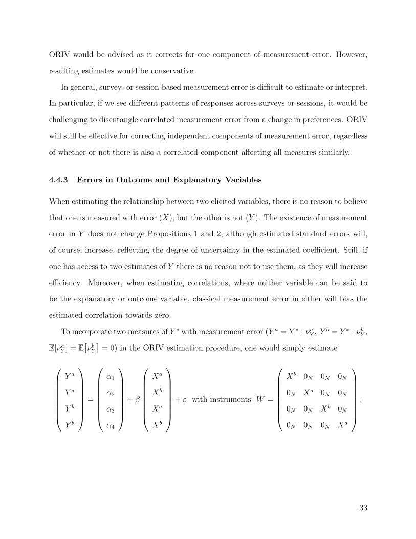
ORIV would be advised as it corrects for one component of measurement error. However,

resulting estimates would be conservative.

In general, survey- or session-based measurement error is difficult to estimate or interpret.

In particular, if we see different patterns of responses across surveys or sessions, it would be

challenging to disentangle correlated measurement error from a change in preferences. ORIV

will still be effective for correcting independent components of measurement error, regardless

of whether or not there is also a correlated component affecting all measures similarly.

4.4.3 Errors in Outcome and Explanatory Variables

When estimating the relationship between two elicited variables, there is no reason to believe

that one is measured with error (X), but the other is not (Y ). The existence of measurement

error in Y does not change Propositions 1 and 2, although estimated standard errors will,

of course, increase, reflecting the degree of uncertainty in the estimated coefficient. Still, if

one has access to two estimates of Y there is no reason not to use them, as they will increase

efficiency. Moreover, when estimating correlations, where neither variable can be said to

be the explanatory or outcome variable, classical measurement error in either will bias the

estimated correlation towards zero.

To incorporate two measures of Y ∗ with measurement error (Y a = Y ∗+νaY , Yb = Y ∗+νbY ,

E[νaY ] = E[νbY]

= 0) in the ORIV estimation procedure, one would simply estimate

Y a

Y a

Y b

Y b

=

α1

α2

α3

α4

+ β

Xa

Xb

Xa

Xb

+ ε with instruments W =

Xb 0N 0N 0N

0N Xa 0N 0N

0N 0N Xb 0N

0N 0N 0N Xa

.

33

4.4.4 Estimating Correlations from Consistent Coefficients

ORIV produces β∗, a consistent estimate of β∗. Notice that

β =Cov[X, Y ]

Var[X]implying ρXY = β

√√√√Var[X]

Var[Y ],

where ρXY is the correlation. Thus, we need consistent estimates of Var[X∗] and Var[Y ∗]

to recover ρ∗XY . The problem is that Var[X] = Var[X∗] + Var[νX ]. As Var[Y ] is biased as

well, it is not clear if transforming the regression coefficient into a correlation will generate

an estimate that is biased up or down. Nonetheless, we have

Cov[Xa, Xb] = Cov[X∗ + νaX , X∗ + νbX ] = Var[X∗] so ρ∗XY = β∗

√√√√Cov[Xa, Xb]

Cov[Y a, Y b].

Proposition 3. ρ∗XY is consistent with an asymptotically normal distribution, where stan-

dard errors can be derived using the delta method. These standard errors can be consistently

estimated using a bootstrap to construct confidence intervals.

An example of how to estimate correlations and bootstrapped standard errors using

ORIV in STATA can be found in Appendix C. A STATA program to estimate correlations

and bootstrapped standard errors is available from the authors upon request.

4.5 Corrected Correlations between Risk Elicitation Techniques

We now use ORIV estimators to examine the correlations between different risk measures.

Table 6 contains both the raw and corrected correlations. Both the Risk MPL and the

Project measures were elicited twice. The qualitative risk assessment was elicited once in

the Fall of 2014 and again in the Spring of 2015, the latter serving as the duplicate elicitation.

34

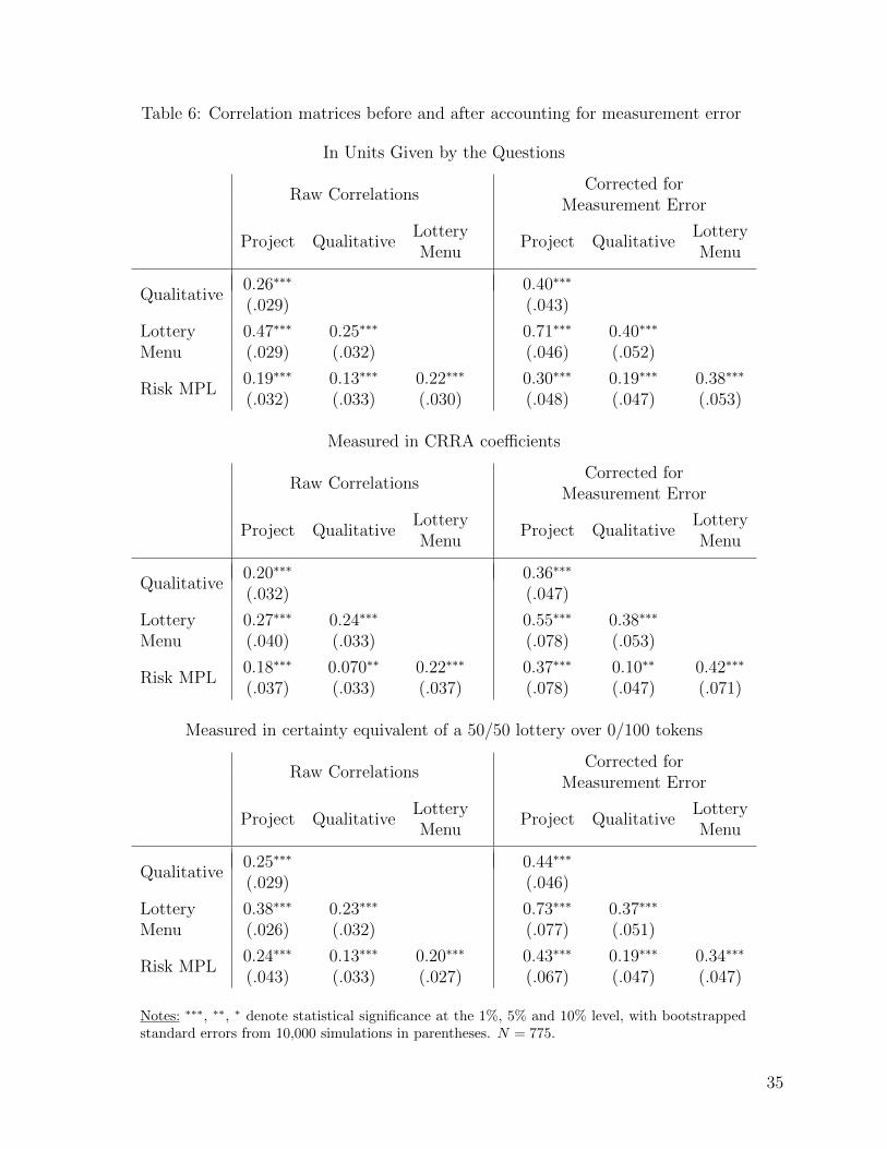
Table 6: Correlation matrices before and after accounting for measurement error

In Units Given by the Questions

Raw CorrelationsCorrected for

Measurement Error

Project QualitativeLottery


Menu Menu

Qualitative0.26∗∗∗ 0.40∗∗∗

(.029) (.043)

Lottery 0.47∗∗∗ 0.25∗∗∗ 0.71∗∗∗ 0.40∗∗∗

Menu (.029) (.032) (.046) (.052)

Risk MPL0.19∗∗∗ 0.13∗∗∗ 0.22∗∗∗ 0.30∗∗∗ 0.19∗∗∗ 0.38∗∗∗

(.032) (.033) (.030) (.048) (.047) (.053)

Measured in CRRA coefficients


Measurement Error



Menu Menu


(.032) (.047)

Lottery 0.27∗∗∗ 0.24∗∗∗ 0.55∗∗∗ 0.38∗∗∗

Menu (.040) (.033) (.078) (.053)

Risk MPL0.18∗∗∗ 0.070∗∗ 0.22∗∗∗ 0.37∗∗∗ 0.10∗∗ 0.42∗∗∗

(.037) (.033) (.037) (.078) (.047) (.071)

Measured in certainty equivalent of a 50/50 lottery over 0/100 tokens


Measurement Error



Menu Menu


(.029) (.046)

Lottery 0.38∗∗∗ 0.23∗∗∗ 0.73∗∗∗ 0.37∗∗∗

Menu (.026) (.032) (.077) (.051)

Risk MPL0.24∗∗∗ 0.13∗∗∗ 0.20∗∗∗ 0.43∗∗∗ 0.19∗∗∗ 0.34∗∗∗

(.043) (.033) (.027) (.067) (.047) (.047)

Notes: ∗∗∗, ∗∗, ∗ denote statistical significance at the 1%, 5% and 10% level, with bootstrappedstandard errors from 10,000 simulations in parentheses. N = 775.

35

The Lottery Menu measure was elicited only once.32

Previous work comparing different risk-elicitation techniques often transforms them into

a common scale (see Deck et al., 2010, for an example). For comparability, we do the same

in Table 6. This is not theoretically advisable as it introduces a non-linear change in the

structure of measurement error, which may lead to inconsistent estimates. However, for the

question at hand, this makes little difference in the results.

In the top panel, we consider correlations between the unaltered measures. That is,

we use units given by the elicitation techniques. The second panel translates these various

measures into CRRA coefficients, except for the qualitative assessment, which does not lend

itself to transformation. The third panel uses the imputed CRRA coefficients to calculate

the implied certainty equivalent with a 50% probability of 100 tokens and a 50% probability

of 0 tokens. Note that in the case of the Risk MPLs, this is the same as the questions’

natural units, as these are elicitations of certainty equivalents over 50/50 lotteries.

All three panels suggest similar conclusions. First, the corrected correlations are sub-

stantially higher. While the raw correlations are arguably low, never exceeding 0.5 (and

uniformly below 0.27 when considering imputed CRRA coefficients), corrected correlations

are dramatically higher, reaching levels as high as 0.73. Whether this correlation is “high” or

“low” is largely a judgement call. However, the literature seems to consistently suggest that

correlations above 0.7 are very high (see, for example, Cohen, 1988; Evans, 1996). Moreover,

many perceived strong links correspond to correlations that are 0.7 or below. For exam-

ple, the correlation between parents’ and their childrens’ heights hovers around 0.5 (Wright

and Cheetham, 1999), the correlation between height and foot length for individuals over

the age of 30 is about 0.6 for females and 0.7 for males (Pawar and Dadhich, 2012), the

correlation between average parents’ education and their children’s education ranges from

32For correlations involving the Lottery Menu task, we multiply by

√Var[((Xa)′ (Xb)′)′]/Var[Y ]. This

is valid so long as the measurement error in the measures of X and Y are equal—that is, so long asCorr[Xa, Xb] = Var[Y ∗]/Var[Y ], as shown in (4). Having only one measure of Y , we have no measure ofVar[Y ∗], and cannot test this. However, the correlation between elicitations for the three that we do haveare 0.67 (s.e. 0.027, projects), 0.62 (s.e. 0.028, qualitative), and 0.59 (s.e. 0.29, Risk MPLs), so this seemsreasonable.

36

around 0.30 in Denmark and 0.54 in Italy, with most western countries falling somewhere

in-between (Hertz et al., 2007), and the correlation between Body Mass Index (BMI) and

insulin resistance—which underlies the link between obesity and type-2 diabetes—is around

0.46 (Abbasi et al., 2002). Second, some measures are noticeably more correlated. Namely,

the Project measure appears to be most correlated with the other elicitation techniques. It is

most highly correlated with the Lottery Menu measure, with corrected correlations of 0.55–

0.73, depending on the units of measurement. The Lottery Menu also exhibits relatively

high correlations with the other measures. The lowest correlations are observed between the

Risk MPL and the Qualitative measure.

4.6 Substantive Implications

There are good reasons to suspect that the Risk MPL measure captures risk attitudes over

a different domain than the other measures: its smaller correlation with other measures,

and the fact that, unlike other risk measures, it is uncorrelated with gender, as shown in

Figure 1. In that figure, the average risk attitudes of men and women are very close when

considering the Risk MPLs, but all other measures show that women are substantially more

risk averse than men.33 These differences account for the explanatory power of risk controls

on the gender gap in competitiveness in Section 3.2.

The fact that different measures yield different conclusions about the relationship be-

tween gender and risk attitudes is reflected in the behavioral literature, which reaches mixed

conclusions about the general relationship between gender and risk (see, for example, Byrnes,

Miller, and Schafer, 1999, for a review of the relevant experimental work in psychology, and

Croson and Gneezy, 2009; Eckel and Grossman, 2008b; and Niederle, 2015, for reviews of

related experimental work in economics).34 On the other hand, the finance literature has

found a more consistent difference between men and women when considering risky finan-

33In addition to the usual concerns with the Kolmogorov-Smirnov test, it is not valid for discrete distri-butions. In such cases, the p-value is only approximate, and may lead to extreme implications, such as thep-values of 1.000 found in Figure 2. As such, we provide p-values only to aid visual inspection.

34Our findings are consistent with some observations in Holt and Laury (2014).

37

cial investments (see, for example, Barber and Odean, 2013; Embrey and Fox, 1997; Farrell,

2011). The Project measure intentionally mimics a stock/bond portfolio choice (or risky/safe

assets), and the gender-based behavior in this task is similar to that seen in real financial

investments: men invest more aggressively than women.35

There is also variation in the consistency of responses to the different risk elicitation

techniques across time. The Project task, Risk MPL, and Qualitative assessment were all

elicited in both the Fall 2014 and Spring 2015 installments of the survey. The risk attitudes

elicited by the Project task exhibit more stability than the Risk MPLs—a correlation of

0.65 (0.038) for the Project measure(s), compared with 0.42 (0.063) for the Risk MPL (both

corrected for measurement error). The Qualitative elicitation was performed only once per

survey, and the uncorrected correlation between these elicitations was 0.62.

Taken together, these different measures may be representative of risk attitudes in differ-

ent settings. This would not be surprising, as psychologists have found that risk attitudes

do differ across contexts (Slovic, 1964; see Kruger, Wang, and Wilke, 2007; Weber, Blais,

and Betz, 2002; and references therein for more recent work). While there are many criteria

on which one might evaluate such measures, the Project-based measure seems particularly

attractive due to its stability, correlation with other popular measures, and the fact that the

literal interpretation of the measure is consistent with evidence from the field, in finance.36

The next section uses the ORIV technique to examine risk in a particular domain—

compound lotteries—and how it relates to ambiguous (uncertain) lotteries.

35The lotteries in the Lottery Menu task can be viewed as corresponding to different investment allocationsbetween a safe option and a risky one that pays three times the amount invested with 50% probability, seeEckel and Grossman (2002). Eckel and Grossman (2008a) observed that results are not sensitive to whetheror not lotteries are described as risky investments to participants, which is consistent with the Lottery Menutask exhibiting similar patterns to the Project measure.

36Recent evidence suggests the presence of a global risk component that explains individuals’ choices acrossinvestment domains. This component exhibits some of the features of the Project measure (Einav et al.,2012).

38

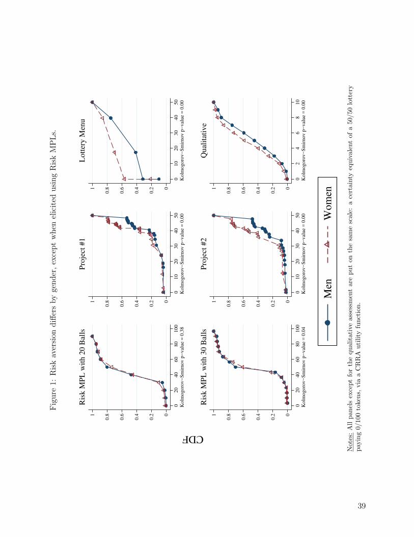
Fig

ure

1:R

isk

aver

sion

diff

ers

by

gender

,ex

cept

when

elic

ited

usi

ng

Ris

kM

PL

s.

0

0.2

0.4

0.6

0.81

020

40

60

80

100

Kolm

ogoro

v−

Sm

irnov p

−val

ue

= 0

.38

Ris

k M

PL

wit

h 2

0 B

alls

0

0.2

0.4

0.6

0.81

010

20

30

40

50

Kolm

ogoro

v−

Sm

irnov p

−val

ue

= 0

.00

Pro

ject

#1

0

0.2

0.4

0.6

0.81

010

20

30

40

50

Kolm

ogoro

v−

Sm

irnov p

−val

ue

= 0

.00

Lo

tter

y M

enu

0

0.2

0.4

0.6

0.81

020

40

60

80

100

Kolm

ogoro

v−

Sm

irnov p

−val

ue

= 0

.04

Ris

k M

PL

wit

h 3

0 B

alls

0

0.2

0.4

0.6

0.81

010

20

30

40

50

Kolm

ogoro

v−

Sm

irnov p

−val

ue

= 0

.00

Pro

ject

#2

0

0.2

0.4

0.6

0.81

02

46

810

Kolm

ogoro

v−

Sm

irnov p

−val

ue

= 0

.00

Qu

alit

ativ

e

CDF

Men

Wo

men

Not

es:

All

pan

els

exce

pt

for

the

qu

ali

tati

veass

essm

ent

are

pu

ton

the

sam

esc

ale

:a

cert

ain

tyeq

uiv

ale

nt

of

a50/50

lott

ery

pay

ing

0/10

0to

ken

s,via

aC

RR

Au

tili

tyfu

nct

ion

.

39

5 New Traits

Measurement error may lead researchers to believe that an observed behavior is not well

explained by current theory. We have already shown one example of this in Section 3:

using controls that are measured with error may lead researchers to believe a behavior is

independent of other behaviors. It is natural to think that bias in correlations, explored in

the last section, may similarly cause researchers to underestimate the relationship between

two variables, and thus declare them distinct when they are, in fact, not. In this section we

provide a potential example of this phenomenon by examining attitudes towards ambiguity.

Ambiguity aversion refers to a preference for known risks over unknown risks. First

introduced by Ellsberg (1961), this preference implies that an ambiguity averse individual

would prefer a lottery with a known probability distribution of rewards over a similar lottery

in which the probability distribution of rewards is unknown. This behavior is expressed in

the Ellsberg Paradox, where participants prefer a bet on the draw of a black ball from an

urn with, say, 10 red and 10 black balls than on one with 20 total balls, but with unknown

composition. Ambiguity aversion is widely studied, and used to explain incomplete contracts,

volatility in stock markets, selective abstention in elections, and so on (Mukerji, 2000).

Segal (1987, 1990) suggests that choices under ambiguity may come from improperly

compounding a sequence of lotteries. For instance, in the Ellsberg Paradox scenario above,

a participant might view a draw from the ambiguous urn as having two stages: First, the

number of red balls is randomly determined, according to some subjective probability; sec-

ond, a ball is drawn from the urn. If an individual fails to properly reduce these two lotteries

into one, a bias will result. Halevy (2007) experimentally tests this proposition. In his study,

participants face both an Ellsberg urn, and an urn where the number of red balls is uniformly

determined. In his results, Halevy reports correlations of around 0.5 between behaviors in

both treatments. Nonetheless, his results suggest that half the variation in the responses

to ambiguous and compound lotteries is independent. This implies a strong, but imperfect,

link between ambiguity aversion and (negative) reactions to compound lotteries.

40

In this section, we replicate Halevy’s exercise, adding duplicate measures of certainty

equivalents of both ambiguous and compound lotteries. This allows us to correct for mea-

surement error using ORIV. As a result, ambiguity aversion and reaction to compound

lotteries appear almost identical.

5.1 Ambiguity Aversion and Reaction to Compound Lotteries

As described in Section 3.1, the Risk MPL, Compound MPL, and Ambiguous MPL are all

implemented in a very similar way. All ask for a participant’s certainty equivalent value of a

draw from an urn if a certain color ball is drawn. All allow the participant to select the color

of the ball associated with positive payment. All have the same number of balls, and the same

payoff. The only difference is how the distribution of balls in the urn is specified: half black

and half red for Risk; drawn from a uniform distribution for Compound; or unknown, but

selected by the Dean of Undergraduate Students for Ambiguous. Each measure is replicated

twice: once with a 20-ball urn and a payoff of 100 tokens if the correct color ball is drawn,

and once with a 30-ball urn and a 150-token payoff.

Our data show evidence of ambiguity aversion, as well as a negative reaction to compound

lotteries. In particular, the certainty equivalents of the ambiguous urns are 2.5 (0.48) and

2.5 (0.46) percentage points lower than those of the risky urns for the 20 and 30 ball urns,

respectively; and the certainty equivalents of the compound lotteries are 2.9 (0.51) and 2.8

(0.51) percentage points lower than those of the risky urns. Note that these differences are

statistically significant, but they are not statistically significantly different from each other.

On average, ambiguity aversion and reaction to compound lotteries are identical.37

Table 7 reports the raw and corrected correlations between the three measures. The raw

correlation between ambiguous and compound certainty equivalents are 0.65. This is in line

37On the individual level, 30% of our respondents prefer the uncertain lottery over the ambiguous one, 20%prefer the ambiguous lottery, and 50% are neutral. Halevy (2007) used the BDM method to elicit certaintyequivalents, whereas we use an MPL. This choice was made because MPLs are easier to explain on a survey,when participants are not able to ask the experimenter for help. Once we take into account the fact thatparticipants in our experiment express certainty equivalents in units 20 times as large as Halevy (2007), hisdata, which he graciously provided to us, is reasonably close to ours.

41

Table 7: The correlation between certainty equivalents is substantial.


Measurement Error

Risk Compound Compound Risk Compound CompoundCE CE Reaction CE CE Reaction

Compound 0.55∗∗∗ 0.74∗∗∗

CE (.035) (.043)

Ambiguous 0.60∗∗∗ 0.65∗∗∗ 0.78∗∗∗ 0.85∗∗∗

CE (.033) (.027) (.037) (.029)

Ambiguity 0.44∗∗∗ 0.86∗∗∗

Aversion (.039) (.059)

Notes: ∗∗∗, ∗∗, ∗ denote statistical significance at the 1%, 5%, and 10% level, with bootstrapped standarderrors from 10,000 simulations in parentheses. N = 774.

with Halevy (2007), who reports a correlation of 0.45 in the first round of his experiment, and

a correlation of 0.71 in his robustness round. However, once measurement error is corrected

for in our study, the correlation is much higher: 0.85.

Corrected correlations between certainty equivalents of risky and compound or ambiguous

urns are substantial as well: estimated at 0.74 and 0.78, respectively. This leads to an

important point: the high correlation between ambiguity aversion and reaction to compound

lotteries may be because the certainty equivalents of both reflect risk attitudes as well.

Thus, we subtract the risk certainty equivalents from each of the compound and ambiguous

certainty equivalents, leaving measures of ambiguity aversion, and (negative) reaction to

compound lotteries. This results in a smaller raw correlation of 0.44, but the same correlation

of 0.86 when measurement error is taken into account. Moreover, the 95% confidence interval

for this value is (0.74, 0.98). Thus, while we can reject the null hypothesis that the correlation

is 1, we cannot reject the null that the correlation is very close to 1.38

Here, unlike in Section 3, our large sample size is likely the reason we find any difference

at all. Drawing a random sample of 104 observations (the size of Halevy’s experiment) 10,000

38The 99% confidence interval is (0.71, 1.01). Halevy’s data has a correlation 0.47 in the main experiment,and 0.75 in the robustness round.

42

times, the correlation between ambiguity aversion and reaction to compound lotteries differs

from 1 only 1.2% of the time at the 1% level, 4.8% of the time at the 5% level, and 9.0%

of the time at the 10% level. It should be noted that these are the results from standard

confidence intervals that are well-calibrated. While correlations have an upper bound of 1,

and thus suffer from the Andrews’s (2001) problem, our estimator can take on values greater

than 1, and is normally distributed around 1 when that is the true correlation. Thus, any

time a correlation greater than 1 is calculated using ORIV, this should be interpreted as

strong evidence that the correlation is actually 1, rather than as a statistical issue.

As a final way of showing how closely ambiguity aversion and reaction to compound

lotteries are related, we plot the CDFs of the various measures in Figure 2. The left-most

panels show certainty equivalents for risky urns and ambiguous urns—the fact that these

diverge below 50 is evidence of ambiguity aversion. The center panels show the certainty

equivalents for ambiguous urns and compound urns: the distributions appear identical. The

final panels show the distributions of ambiguity aversion and reaction to compound lotteries.

Once again, these appear identical.

5.2 Substantive Implications

Ambiguity aversion and reaction to compound lotteries appear remarkably similar once mea-

surement error is accounted for. It is worth noting that this is compatible with the original

description of Knightian (1921) Uncertainty,

[T]he essential fact is that “risk” means in some cases a quantity susceptible ofmeasurement, while at other times it is something distinctly not of this char-acter; and there are far-reaching and crucial differences in the bearings of thephenomena depending on which of the two is really present and operating.

That is, compound lotteries may be no more “susceptible to measurement” for individuals—

even Caltech students, who are mathematically inclined—than those that are ambiguous.

This suggests to us that the defining characteristic—in addition to risk attitudes—in

determining valuations of these lotteries is some notion of complexity. Regardless of the

43

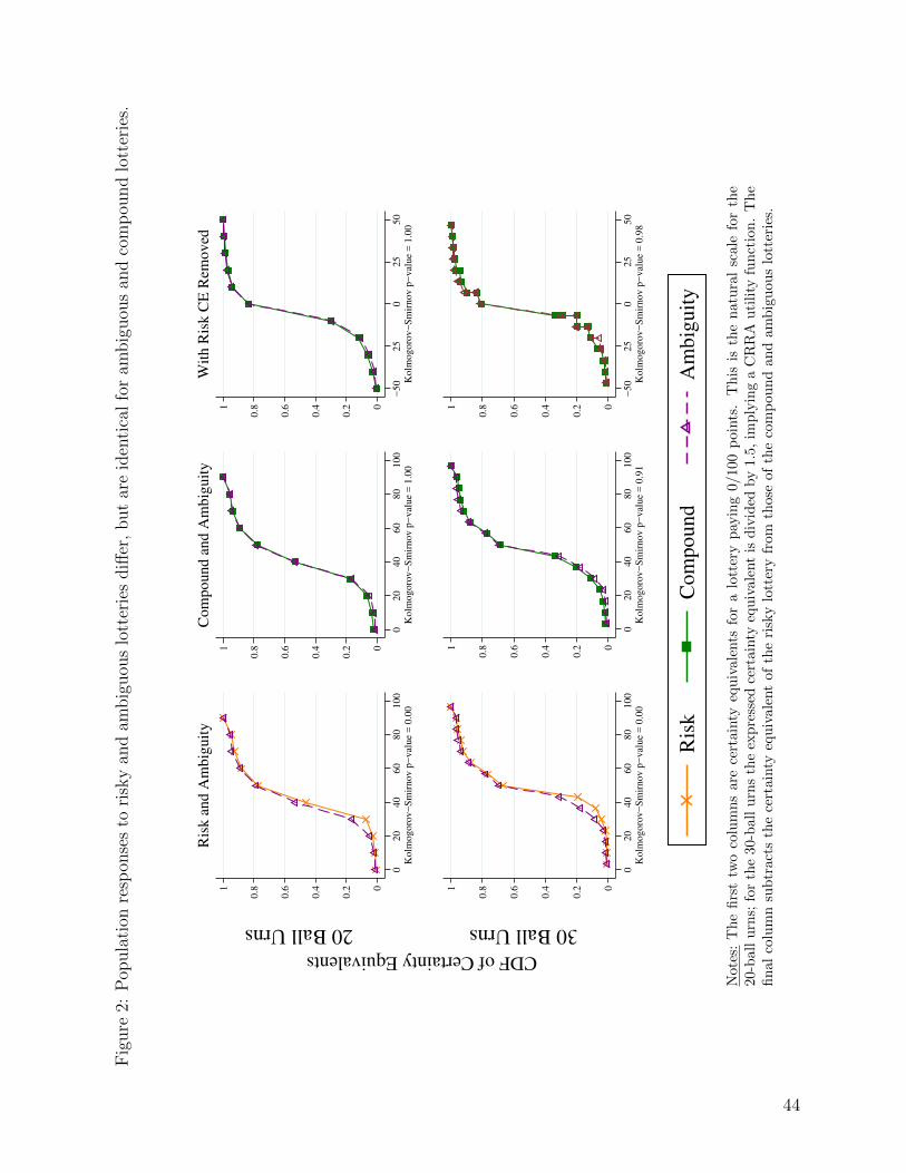
Fig

ure

2:P

opula

tion

resp

onse

sto

risk

yan

dam

big

uou

slo

tter

ies

diff

er,

but

are

iden

tica

lfo

ram

big

uou

san

dco

mp

ound

lott

erie

s.

0

0.2

0.4

0.6

0.81

020

40

60

80

100

Kolm

ogoro

v−

Sm

irnov p

−val

ue

= 0

.00

Ris

k a

nd

Am

big

uit

y

0

0.2

0.4

0.6

0.81

020

40

60

80

100

Kolm

ogoro

v−

Sm

irnov p

−val

ue

= 1

.00

Co

mp

ou

nd

an

d A

mb

igu

ity

0

0.2

0.4

0.6

0.81

−50

25

025

50

Kolm

ogoro

v−

Sm

irnov p

−val

ue

= 1

.00

Wit

h R

isk

CE

Rem

ov

ed

0

0.2

0.4

0.6

0.81

020

40

60

80

100

Kolm

ogoro

v−

Sm

irnov p

−val

ue

= 0

.00

0

0.2

0.4

0.6

0.81

020

40

60

80

100

Kolm

ogoro

v−

Sm

irnov p

−val

ue

= 0

.91

0

0.2

0.4

0.6

0.81

−50

25

025

50

Kolm

ogoro

v−

Sm

irnov p

−val

ue

= 0

.98

30 Ball Urns 20 Ball Urns

CDF of Certainty Equivalents

Ris

kC

om

pound

Am

big

uit

y

Not

es:

Th

efi

rst

two

colu

mn

sar

ece

rtain

tyeq

uiv

ale

nts

for

alo

tter

yp

ayin

g0/100

poin

ts.

Th

isis

the

natu

ral

scale

for

the

20-b

all

urn

s;fo

rth

e30

-bal

lu

rns

the

exp

ress

edce

rtain

tyeq

uiv

ale

nt

isd

ivid

edby

1.5

,im

ply

ing

aC

RR

Au

tili

tyfu

nct

ion.

Th

efi

nal

colu

mn

sub

trac

tsth

ece

rtai

nty

equ

ivale

nt

of

the

risk

ylo

tter

yfr

om

those

of

the

com

pou

nd

an

dam

big

uou

slo

tter

ies.

44

philosophical interpretation of these results, it is clear that any successful model of ambiguity

aversion should also predict behavior in complex, but fully specified, risky environments.

6 Conclusion

If measurement error is such a ubiquitous, but easily correctable, issue, why has the ex-

perimental literature paid so little attention to it? The answer likely lies in the fact that

attenuation bias driven by measurement error is a conservative bias. That is, it biases the

researcher against false positives. So when asked about measurement error, a researcher can

confidently answer that it would “go against finding anything.”

However, measurement error creates another, field-wide, issue that has been little appre-

ciated. It leads to the over-identification of “new” phenomena. Indeed, our paper shows two

examples of this: previously, competitiveness was thought to have a component unconnected

to risk aversion and overconfidence, and ambiguity aversion and reaction to compound lot-

teries (the latter a form of risk aversion) were thought to be distinct. Our results show that

both are unlikely to be true. Moreover, our finding that elicitations of risk attitudes are

more highly correlated than previously appreciated suggests that fewer elicitation methods

are needed than previously thought. Given that these are the only three results we have ex-

amined in trying to understand the influence of measurement error in experiments, it seems

likely that the over-identification of new phenomena is a substantial problem.

That measurement error may lead to the identification of new phenomena where none

exist may feed into the recent mushrooming of methodological work suggesting the high rates

of non-replicability of research discoveries (see Ioannidis, 2005; Simonsohn, 2015, and refer-

ences therein). Using the techniques developed here to account for measurement error may

help researchers discover, in a more robust fashion, the deep connections between different

attitudes and effects.

45

References

Abbasi, Fahim, Byron William Brown, Cindy Lamendola, Tracey McLaughlin, and Gerald MReaven. 2002. “Relationship between Obesity, Insulin Resistance, and Coronary HeartDisease Risk.” Journal of the American College of Cardiology 40 (5):937–943.

Adcock, Robert James. 1878. “A Problem in Least Squares.” The Analyst 5 (2):53–54.

Agranov, Marina and Leeat Yariv. 2015. “Collusion through Communication in Auctions.”California Institute of Technology, mimeo.

Aguiar, Victor and Nail Kashaev. 2017. “Stochastic Revealed Preferences with Measure-ment Error: Testing for Exponential Discounting in Survey Data.” University of WesternOntario, mimeo.

Ambuehl, Sandro and Shengwu Li. 2015. “Belief Updating and the Demand for Information.”Stanford University, mimeo.

Anderson, Lisa R. and Jennifer M. Mellor. 2009. “Are Risk Preferences Stable? Comparingan Experimental Measure with a Validated Survey-based Measure.” Journal of Risk andUncertainty 39 (2):137–160.

Andrews, Donald W.K. 2001. “Testing when a Parameter is on the Boundary of the Main-tained Hypothesis.” Econometrica 68 (2):683–734.

Angrist, Joshua and Alan B. Krueger. 2001. “Instrumental Variables and the Search forIdentification: From Supply and Demand to Natural Experiments.” Journal of EconomicPerspectives 15 (4):69–85.

Barber, Brad M. and Terrance Odean. 2013. “The Behavior of Individual Investors.” InHandbook of Economics of Finance, vol. 2B: Asset Pricing, edited by George M. Constan-tinides, Milton Harris, and Rene M. Stulz. Oxford, UK: North-Holland, 1533–1570.

Battalio, Raymond C., John H. Kagel, Robin C. Winkler, Edwin B. Fisher, Robert L. Bas-mann, and Leonard Krasner. 1973. “A Test of Consumer Demand Theory using Observa-tions of Individual Consumer Purchases.” Western Economic Journal 11 (4):411–428.

Beauchamp, Jonathan, David Cesarini, and Magnus Johannesson. 2015. “The Psychometricand Empirical Properties of Measures of Risk Preferences.” University of Toronto, mimeo.

Belloni, Alexandre, Victor Chernozhukov, and Christian Hansen. 2013. “Inference on Treat-ment Effects after Selection among High-Dimensional Controls.” Review of EconomicStudies 81 (2):608–650.

Belloni, Alexandre, Victor Chernozhukov, and Lie Wang. 2011. “Square-Root LASSO: Piv-otal Recovery of Sparse Signals via Conic Programming.” Biometrika 98 (4):791–806.

Bertrand, Marianne and Sendhil Mullainathan. 2001. “Do People Mean what they Say?Implications for Subjective Survey Data.” American Economic Review (Papers & Pro-ceedings) 91 (2):67–72.

References–1

Blattman, Christopher, Julian C. Jamison, Tricia Koroknay-Palicz, Katherine Rodrigues,and Margaret Sheridan. 2015. “Measuring the Measurement Error: A Method to Quali-tatively Validate Survey Data.” NBER Working Paper Series # 21447.

Bound, John, Charles Brown, and Nancy Mathiowetz. 2001. “Measurement Error in SurveyData.” In Handbook of Econometrics, vol. 5, edited by James J. Heckman, chap. 59.Amsterdam, The Netherlands: Elsevier, 3705–3843.

Buonaccorsi, John P. 2010. Measurement Error: Models, Methods, and Applications. BocaRaton, Florida: CRC Press.

Buser, Thomas, Muriel Niederle, and Hessel Oosterbeek. 2014. “Gender, Competitiveness,and Career Choices.” Quarterly Journal of Economics 129 (3):1409–1447.

Byrnes, James P, David C Miller, and William D Schafer. 1999. “Gender Differences in RiskTaking: A Meta-analysis.” Psychological Bulletin 125 (3):367–383.

Candes, Emmanuel and Terence Tao. 2007. “The Dantzig Selector: Statistical Estimationwhen p is much Larger than n.” Annals of Statistics 35 (6):2313–2351. URL http:

//dx.doi.org/10.1214/009053606000001523.

Carroll, Raymond J. and Leonard A. Stefanski. 1994. “Measurement Error, InstrumentalVariables and Corrections for Attenuation with Applications to Meta-analyses.” Statisticsin Medicine 13 (12):1265–1282.

Castillo, Marco, Jeffrey L. Jordan, and Ragan Petrie. 2015. “Children’s Rationality, RiskAttitudes, and Misbehavior.” George Mason University, mimeo.

Charness, Gary, Uri Gneezy, and Alex Imas. 2013. “Experimental Methods: Eliciting RiskPreferences.” Journal of Economic Behavior & Organization 87 (1):43–51.

Cleave, Blair L, Nikos Nikiforakis, and Robert Slonim. 2013. “Is there Selection Bias in Lab-oratory Experiments? The Case of Social and Risk Preferences.” Experimental Economics16 (3):372–382.

Coffman, Lucas and Paul Niehaus. 2015. “Pathways to Persuasion.” Ohio State University,mimeo.

Cohen, Jacob. 1988. Statistical Power Analysis for the Behavioral Sciences. Mahwah, NewJersey: Lawrence Earlbaum Associates, 2nd edition ed.

Condon, David M and William Revelle. 2014. “The International Cognitive Ability Resource:Development and Initial Validation of a Public-domain Measure.” Intelligence 43 (2):52–64.

Croson, Rachel and Uri Gneezy. 2009. “Gender Differences in Preferences.” Journal ofEconomic Literature 47 (2):448–474.

References–2

http://dx.doi.org/10.1214/009053606000001523

http://dx.doi.org/10.1214/009053606000001523

Dave, Chetan, Catherine C. Eckel, Cathleen A. Johnson, and Christian Rojas. 2010. “Elicit-ing risk preferences: When is simple better?” Journal of Risk and Uncertainty 41 (3):219–243.

Dean, Mark and Pietro Ortoleva. 2016. “Is it All Connected? A Testing Ground for UnifiedTheories of Behavioral Economics Phenomena.” Columbia University, mimeo.

Deck, Cary, Jungmin Lee, Javier Reyes, and Chris Rosen. 2010. “Measuring Risk Aversionon Multiple Tasks: Can Domain Specific Risk Attitudes Explain Apparently InconsistentBehavior?” University of Arkansas, mimeo.

Deck, Cary A., Jungmin Lee, Javier A. Reyes, and Chris Rosen. 2008. “Measuring RiskAttitudes Controlling for Personality Traits.” SSRN working paper #1148521.

Dohmen, Thomas, Armin Falk, David Huffman, Uwe Sunde, Jurgen Schupp, and Gert GWagner. 2011. “Individual Risk Attitudes: Measurement, Determinants, and BehavioralConsequences.” Journal of the European Economic Association 9 (3):522–550.

Drerup, Tilman, Benjamin Enke, and Hans-Martin von Gaudecker. 2016. “The Precision ofSubjective Data and the Explanatory Power of Economic Models.” Harvard University,mimeo.

Durbin, James. 1954. “Errors in Variables.” Revue de l’Institut International de Statistique22 (1/3):23–32.

Eckel, Catherine C. and Philip J. Grossman. 2002. “Sex Differences and Statistical Stereotyp-ing in Attitudes toward Financial Risk.” Evolution and Human Behavior 23 (4):281–295.

———. 2008a. “Forecasting Risk Attitudes: An Experimental Study Using Actual andForecast Gamble Choices.” Journal of Economic Behavior & Organization 68 (1):1–17.

Eckel, Catherine C and Philip J Grossman. 2008b. “Men, Women and Risk Aversion: Ex-perimental Evidence.” In Handbook of Experimental Economics Results, vol. 1, edited byCharles R. Plott and Vernon L. Smith. North-Holland, 1061–1073.

Einav, Liran, Amy Finkelstein, Iuliana Pascu, and Mark Cullen. 2012. “How General AreRisk Preference? Choices under Uncertainty in Different Domains.” American EconomicReview 101 (2):2606–2638.

Ellsberg, Daniel. 1961. “Risk, Ambiguity, and the Savage Axioms.” The Quarterly Journalof Economics 75 (4):643–669.

Embrey, Lori L. and Jonathan J. Fox. 1997. “Gender Differences in the Investment Decision-making Process.” Financial Counseling and Planning 8 (2):33–40.

Engel, Christoph. 2011. “Dictator Games: A Meta Study.” Experimental Economics14 (4):583–610.

Evans, James D. 1996. Straightforward Statistics for the Behavioral Sciences. Brooks/ColePublishig Company.

References–3

Falk, Armin, Stephan Meier, and Christian Zehnder. 2013. “Do Lab Experiments Misrep-resent Social Preferences? The Case of Self-selected Student Samples.” Journal of theEuropean Economic Association 11 (4):839–852.

Fan, Jianqing and Runze Li. 2001. “Variable Selection via Nonconcave Penalized Likelihoodand its Oracle Properties.” Journal of the American Statistical Association 96 (456):1348–1360.

Fan, Jianqing and Yuan Liao. 2014. “Endogeneity in High Dimensions.” Annals of Statistics42 (3):872–917.

Farrell, James. 2011. “Demographics of Risky Investing.” Research in Business and Eco-nomics Journal Special Edition.

Fiske, Susan T., Daniel T. Gilbert, and Gardner Lindzey. 2010. Handbook of Social Psychol-ogy, vol. 1. Hoboken, NJ: John Wiley & Sons, 5th ed.

Fong, Christina M and Erzo F.P. Luttmer. 2011. “Do Race and Fairness Matter in Generos-ity? Evidence from a Nationally Representative Charity Experiment.” Journal of PublicEconomics 95 (5–6):372–394.

Frederick, Shane. 2005. “Cognitive Reflection and Decision Making.” Journal of EconomicPerspectives 19 (4):25–42.

Friedman, Daniel, R Mark Isaac, Duncan James, and Shyam Sunder. 2014. Risky Curves:On the Empirical Failure of Expected Utility. Routledge.

Friedman, Milton. 1957. A Theory of the Consumtion Function. Princeton, New Jersey:Princeton University Press.

Frisch, Ragnar. 1934. Statistical Confluence analysis by Means of Complete Regression Sys-tems. Universitetets Økonomiske Instituut.

Gneezy, Uri, Muriel Niederle, Aldo Rustichini et al. 2003. “Performance in CompetitiveEnvironments: Gender Differences.” Quarterly Journal of Economics 118 (3):1049–1074.

Gneezy, Uri and Jan Potters. 1997. “An Experiment on Risk Taking and Evaluation Periods.”The Quarterly Journal of Economics 112 (2):631–645.

Goeree, Jacob K., Charles A. Holt, and Thomas R. Palfrey. 2016. Quantal Response Equi-librium: A Stochastic Theory of Games. Princeton University Press.

Greene, William H. 2011. Econometric Analysis. Prentice Hall, 7th ed.

Greenland, Sander. 2000. “An Introduction to Instrumental Variables for Epidemiologists.”International Journal of Epidemiology 29 (4):722–729.

Halevy, Yoram. 2007. “Ellsberg Revisited: An Experimental Study.” Econometrica75 (2):503–536.

References–4

Harless, David W. and Colin F. Camerer. 1994. “The Predictive Utility of CeneralizedExpected Utility Theories.” Econometrica 62 (6):1251–1289.

Harrison, Glenn W, Morten I Lau, and E Elisabet Rutstrom. 2009. “Risk Attitudes, Ran-domization to Treatment, and Self-selection into Experiments.” Journal of EconomicBehavior & Organization 70 (3):498–507.

Hart, Austin and Joel A Middleton. 2014. “Priming Under Fire: Reverse Causality and theClassic Media Priming Hypothesis.” The Journal of Politics 76 (2):581–592.

Hausman, Jerry A. 2001. “Mismeasured Variables in Econometric Analysis: Problems fromthe Right and Problems from the Left.” Journal of Economic Perspectives 15 (4):57–67.

Hertz, Tom, Tamara Jayasundera, Patrizio Piraino, Sibel Selcuk, Nicole Smith, and AlinaVerashchagina. 2007. “The Inheritance of Educational Inequality: International Compar-isons and Fifty-year Trends.” The BE Journal of Economic Analysis & Policy 7 (2):Article10.

Hey, John D. 1991. Experiments in Economics. Blackwell Publishing.

Holt, Charles A. and Susan K. Laury. 2002. “Risk Aversion and Incentive Effects.” AmericanEconomic Review 92 (5):1644–1655.

———. 2014. “Assessment and Estimation of Risk Preferences.” In Handbook of Economicsof Risk and Uncertainty, vol. 1, edited by Mark J. Machina and W. Kip Viscusi. North-Holland, 135–202.

Ioannidis, John P.A. 2005. “Why most Published Research Findings are False.” Chance18 (4):40–47.

Kahneman, Daniel. 1965. “Control of Sprious Association and the Reliability of the Con-trolled Variable.” Psychological Bulletin 54 (5):326–329.

Knight, Frank H. 1921. Risk, Uncertainty and Profit. New York: Hart, Schaffner and Marx.

Koopmans, Tjalling Charles. 1939. Tanker Freight Rates and Tankship Building: An Analysisof Cyclical Fluctuations, by Dr. T. Koopmans. De erven F. Bohn nv.

Kruger, Daniel J., Xiao-Tian Wang, and Andreas Wilke. 2007. “Towards the Developmentof an Evolutionarily Valid Domain-specific Risk-taking Scale.” Evolutionary Psychology5 (3):555–568.

Leeb, Hannes and Benedikt M Potscher. 2005. “Model Selection and Inference: Facts andFiction.” Econometric Theory 21 (1):21–59.

List, John A., Azeem M. Shaikh, and Yang Xu. 2016. “NBER Working Paper #21875.”Multiple Hypothesis Testing in Experimental Economics.

Loomes, Graham. 1991. “Evidence of a New Violation of the Independence Axiom.” Journalof Risk and uncertainty 4 (1):91–108.

References–5

Loomes, Graham and Ganna Pogrebna. 2014. “Measuring Individual Risk Attitudes whenPreferences are Imprecise.” The Economic Journal 124 (576):569–593.

McKelvey, Richard D. and Thomas R. Palfrey. 1995. “Quantal Response Equilibria forNormal Form Games.” Games and Economic Behavior 10 (1):6–38.

———. 1998. “Quantal Response Equilibria for Extensive Form Games.” ExperimentalEconomics 1 (1):9–41.

Moore, Don A. and Paul J. Healy. 2007. “The Trouble with Overconfidence.” CarnegieMellon University, mimeo.

———. 2008. “The Trouble with Overconfidence.” Psychological Review 115 (2):502–517.

Mukerji, Sujoy. 2000. “A Survey of Some Applications of the Idea of Ambiguity Aversion inEconomics.” International Journal of Approximate Reasoning 24 (2–3):221–234.

Nagel, Rosemarie. 1995. “Unraveling in Guessing Games: An Experimental Study.” TheAmerican Economic Review 85 (5):1313–1326.

Niederle, Muriel. 2015. “Gender.” In Handbook of Experimental Economics, Volume 2, editedby John H. Kagel and Alvin E. Roth. Elsevier.

Niederle, Muriel and Lise Vesterlund. 2007. “Do Women Shy Away from Competition? DoMen Compete too Much?” Quarterly Journal of Economics 122 (3):1067–1101.

Ortoleva, Pietro and Erik Snowberg. 2015. “Overconfidence in Political Behavior.” AmericanEconomic Review 105 (2):504–535.

Pawar, Pradeep K and Abhilasha Dadhich. 2012. “Study of Correlation between HumanHeight and Foot Length in Residents of Mumbai.” International Journal of Biological andMedical Research 3 (3):2232–2235.

Raven, James C. 1936. Mental Tests used in Genetic Studies: The Performance of RelatedIndividuals on Tests Mainly Educative and Mainly Reproductive. Ph.D. thesis, Universityof London.

Reiersøl, Olav. 1941. “Confluence Analysis by means of Lag Moments and Other Methodsof Confluence Analysis.” Econometrica 9 (1):1–24.

———. 1945. Confluence Analysis by means of Instrumental Sets of Variables. Stockholm,Sweden: Almqvist & Wiksell.

———. 1950. “Identifiability of a Linear Relation between Variables which are Subject toError.” Econometrica 18 (4):375–389.

Sargan, John D. 1958. “The Estimation of Economic Relationships using InstrumentalVariables.” Econometrica :393–415.

References–6

Segal, Uzi. 1987. “The Ellsberg Paradox and Risk Aversion: An Anticipated Utility Ap-proach.” International Economic Review 28 (1):175–202.

———. 1990. “Two-Stage Lotteries without the Reduction Axiom.” Econometrica58 (2):349–377.

Simonsohn, Uri. 2015. “Small Telescopes: Detectability and the Evaluation of ReplicationResults.” Psychological Science 26 (5):559–569.

Slovic, Paul. 1964. “Assessment of Risk Taking Behavior.” Psychological Bulletin 61 (3):220–233.

Spearman, Charles. 1904. “The Proof and Measurement of Association between TwoThings.” The American Journal of Psychology 15 (1):72–101.

Tibshirani, Robert. 1996. “Regression Shrinkage and Selection via the LASSO.” Journal ofthe Royal Statistical Society. Series B (Methodological) 58 (1):267–288.

Van de Geer, Sara, Peter Buhlmann, Yaacov Ritov, and Ruben Dezeure. 2014. “On Asymp-totically Optimal Confidence Regions and Tests for High-Dimensional Models.” The An-nals of Statistics 42 (3):1166–1202.

van Veldhuizen, Roel. 2016. “Gender Differences in Tournament Choices: Risk Preferences,Overconfidence, or Competitiveness?” WZB Berlin, mimeo.

Wald, Abraham. 1940. “The Fitting of Straight Lines if both Variables are Subject to Error.”The Annals of Mathematical Statistics 11 (3):284–300.

Weber, Elke U., Ann-Renee Blais, and Nancy E. Betz. 2002. “A Domain-specific Risk-attitude Scale: Measuring Risk Perceptions and Risk Behaviors.” Journal of BehavioralDecision Making 15 (4):263–290.

Weizsacker, Georg. 2010. “Do We Follow Others when We Should? A Simple Test of RationalExpectations.” The American Economic Review 100 (5):2340–2360.

Wright, Charlotte M. and Tim D. Cheetham. 1999. “The Strengths and Limitations ofParental Heights as a Predictor of Attained Height.” Archives of Disease in Childhood81 (3):257–260.

References–7

Experimenting with Measurement Error: Techniques...

Documents

Transcript of Experimenting with Measurement Error: Techniques...