Experimentation and theory ofconvective flow in a rotating loop

Item Type text; Thesis-Reproduction (electronic)

Authors Gruca, Walter John, 1941-

Publisher The University of Arizona.

Rights Copyright © is held by the author. Digital access to this materialis made possible by the University Libraries, University of Arizona.Further transmission, reproduction or presentation (such aspublic display or performance) of protected items is prohibitedexcept with permission of the author.

Download date 20/05/2018 20:25:04

Link to Item http://hdl.handle.net/10150/551896

EXPERIMENTATION AND THEORY OF CONVECTIVE FLOW

IN A ROTATING LOOP

by

Walter J. Gruca

t

A Thesis Submitted to the Faculty of the

DEPARTMENT OF NUCLEAR ENGINEERING

In Partial Fulfillment of the Requirements For the Degree of

MASTER OF SCIENCE

In the Graduate College

THE UNIVERSITY OF ARIZONA

1 9 6 7

STATEMENT BY AUTHOR

This thesis has been submitted in partial fulfill­ment of requirements for an advanced degree at The University of Arizona and is deposited in the University Library to be made available to borrowers under rules of the Library.

Brief quotations from this thesis are allowable without special permission, provided that accurate acknowl­edgment of source is made. Requests for permission for extended quotation from or reproduction of this manuscript in whole or in part may be granted by the head of the major department or the Dean of the Graduate College when in his judgment the proposed use of the material is in the inter­ests of scholarship. In all other instances, however, permission must be obtained from the author.

SIGNED:

APPROVAL BY THESIS DIRECTOR

This thesis has been approved on the date shown below:

/)

ROY G. POSTProfessor of Nuclear Engineering

/%%, /~™' Date

ACKNOWLEDGMENTS

The author would like to express special thanks to

Dr o Roy G . Post for his guidance in all aspects of this

research. For the assistance of several other members of

the Department of Nuclear Engineering9 the author is

grateful.

Gratitude is also extended to Mr. Jim Smith for his

technical assistance.

For help in assemblying the rotating loop 9 the

author wishes to acknowledge his father.

Finally9 the writer is thankful for the constant

encouragement and aid of his wife? Jo Ann.

iii

TABLE OF CONTENTS

Page

LIST OF ILLUSTRATIONS ........... . . . . vi

LIST OF TABLES ....................................... vii

ABSTRACT . . . . . . . . . . . . . . viii

INTRODUCTION . . . . . 1

EXPERIMENTAL APPARATUS AND METHODS . . . . . . . . 3

THEORY . . . . . . . . . . . . . . . . . . . . . . 10

Considerations ................................ . 10Temperature 9 Quality 9 Heat Equations . . . . . 12

D erxvatxon . . . . . o . . . . . . . . . . 12Solutions . . . . . . . . . . . . . . . . . l4

Pressure Equations . 15Derivation .................... 15Solutions to the Differential Equation . . 21

DATA ANALYSIS . . ............ 26

Calculating Mass Flow . . . . . . . . . . . . . 26Rotating Loop Equations ......................... 28Observed Mass Flow E q u a t i o n s .................. 31Analytical Equations .............. 3^

RESULTS AND CONCLUSIONS . . . . . . . . . . . . . . 38

Mass Flow-Heat Retention D a t a ........... 38Temperature Data ............................. . 38Mass Flow Data . . . . . . . . . . . . . . . . 43The Coriolis Effect ......... . . . . . . . . . 48Errors . . . . . . . . . . . . . . . 50

Instrumental Errors . . . . . . . . . . . . 50Other Experimental Errors . . . . . . . . . 51Theoretical Errors ......................... 51

Conclusions . . . . . . 52

RECOMMENDATIONS FOR FUTURE WORK . . . . . . . . . . 53

iv

V

TABLE OF CONTENTS— Continued

PageGLOSSARY . . . . . . . . . . . . . . . . ......... 59SELECTED BIBLIOGRAPHY . . . . . ............. . . . 62

LIST OF ILLUSTRATIONS

Figure

1. Schematic of Static L o o p .................. ..

2. Lower Section of Static Loop ..................

3. Overall Rotating Loop . . . . . ........... .

4. Heat Loss With Heat Source ....................

5• Force Diagram of Fluid Flow . . . . . . . . .

6. Fluid Velocity and F l o w ......................

7 . Diagram of Rotating Loop ......................

8 . Rotating Loop Heat Transfer . . . . .........

9• Single Phase Temperatures in Rotating Loop . .

10. Two Phase Temperatures in Rotating Loop . . .

11. Rotating Loop Mass Flow at 0 r.p.m............

12. Rotating Loop Mass Flow at 150 r.p.m. . . . .

13• Rotating Loop Mass Flow at 300 r.p.m..........

14. Static Loop Mass Flow .......................

15• Rotating Loop Mass Flow with Coriolis Effect .

Page

k

5

7

13

17

19

29

3940

41

44

4546

47

49

vi

LIST OF TABLES

Table Page

Ie Temperature, Quality, Heat Equations . l6

IT. Pressure Equations . . . . . . . 22

III o Single Phase S y m b o l s ............ 24

IV. Two Phase Symbols . . . . . . . . . 25

V. Thermal Analysis of Rotating Loop . . . . . . 30

VI o Single Phase Loop Pressure Analysis . . . . . 32

VII . Two Phase Loop Pressure Analysis . . . . . . . 33

vii

ABSTRACT

An experiment was conducted to determine the

importance of Coriolis forces on convection in a rotating

loop. Temperatures of convective fluid flow were measured

for static and rotating systems. Mass flows were calculated

by heat balance and by a mass flow-temperature balance

taking Coriolis forces into account. The Coriolis effect

was assumed to appear as a friction loss. Theoretically,

the pressure drop due to Coriolis forces was demonstrated

to be:

A p = ^^OCu/v'Cr^-r^ ) for single phase

A p - RfjOfWvf (l-X^^ ) (r^-r^. ) for two phase.

The effect of Coriolis forces on the mass flow was

shown to be negligible when the analytical computation was

based on the Bernoulli Equation,

viii

INTRODUCTION

Prolonged voyages in outer space are feasible only

when nuclear power is considered <, For survival in a

hostile element iruch as outer space, heat and electricity

are vital. Nuclear power can supply high electrical and

heat energy, although its weight and space requirements are

optimum only for prolonged periods.

Blinn et al. (1966) have considered cesium and

potassium as working fluids in an advanced high temperature

Rankine cycle power conversion system for space. The study

was conducted for a system to generate one megawatt output

of power. The total weights of the major components of the

power plants compared in this study were 3,894 pounds for

the cesium system and 4,883 pounds for the potassium system.

A 1.5 electrical megawatt thermionic reactor space

power system has been studied by Smith and Parkinson

(1966). Performance potentials of direct conversion from

nuclear heat to electrical power were considered in some

detail. These systems would employ direct nuclear heated

thermionic converters within the reactor fuel elements.

A space electrical power system using nuclear heat

and a magnetohydrodynamic (MED) cycle was studied by

Elliott (1961) and Ulrich and Carter (1963)* High tempera­

ture problems associated with a MED fluid were

1

2

circumvented by using two insoluble fluids: a thermo­

dynamic fluid for thermal to kinetic conversion9 and a

conducting fluid for kinetic to electrical conversion.

One method of obtaining two phase flow for an

orbiting space power system would be to simulate gravity

by rotation. Convection could be induced. Coriolis forces

act on the convective flow in a rotating loop. Measure­

ments of loop parameters and flow would be made to deter­

mine the magnitude of the Coriolis effect.

Experimentation of convection in a rotating loop

was conducted by Stockett (1965) • To measure the convec­

tive fluid flow in centrifugal fields9 an experimental

apparatus was designed^ constructed^ and tested. A heat

transfer loop was rotated about a horizontal axis in a

centrifuge. Temperatures at various locations were

measured by thermocouples. Convective flow was demon­

strated in the rotating loop. Additional experimentation

and analyses of static and rotating loops were necessary

to obtain quantitative data.

EXPERIMENTAL APPARATUS AND METHODS

Convective fluid flow in a static loop and rotating

loop is to be induced and measured, so that the effect of

Coriolis forces can be determined.

The static loop design consisted of a vented glass

tube with thermocouples located at various positions. The

loop was insulated with plastic foam blocks and glass wool.

Figures 1 and 2 show the overall system schematically and

photographically. A heat source and heat sink are located

in the bottom right and top left of the loop respectively.

Iron-constantan thermocouples were connected to a multiple

pole switch which was connected to a single channel Weston

recorder. A rotameter was used to measure the flow of

coolant. A Weston 4^2 Series +.1/2% Electrodynamometer

Type wattmeter was used to measure the heat input at the

heat source.

The rotating loop design consisted of two symmet­

rical vented glass and copper tube loops. Slip rings

transmitted electrical power 9 thermocouple potentials 9 and

valve control signals to or from the rotating loop.

Rotating seals allowed transmission of water to and from

the heat exchangers at the central position of the rotating

loop o The axis of symmetry was the axis of rotation.

Iron-constantan thermocouples were located at important

3

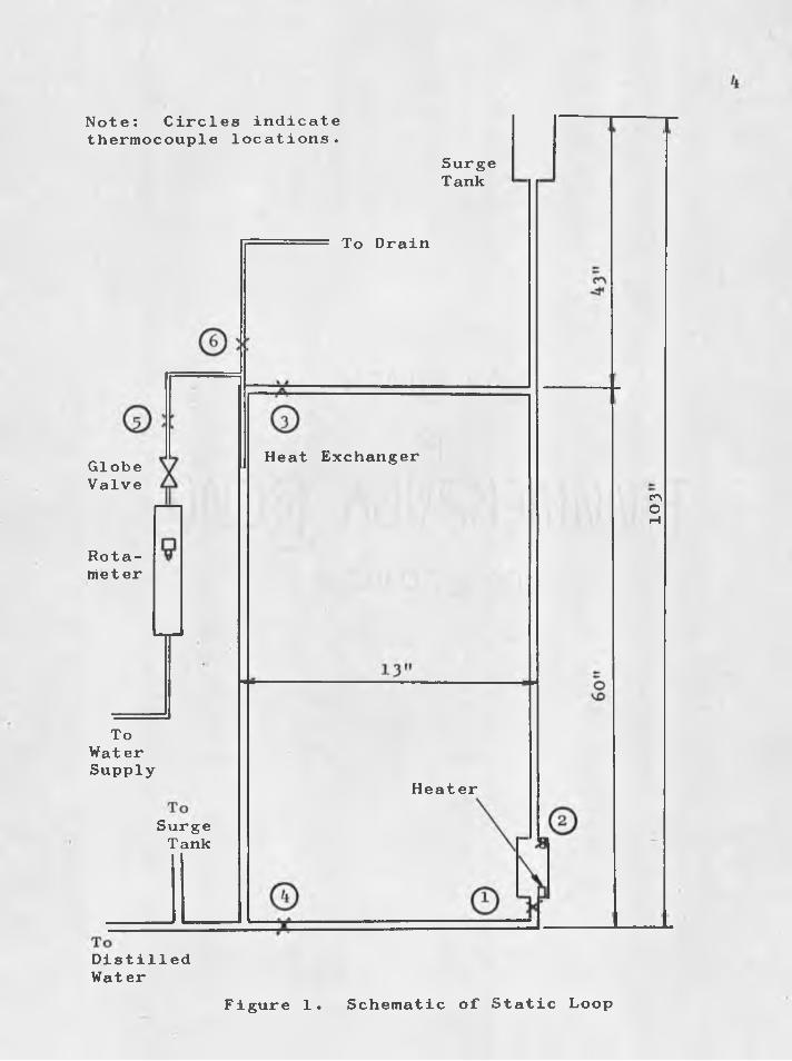
Note: Circles indicatethermocouple locations.

SurgeTank

To Drain

Heat ExchangerGlobeValve

R o t a ­meter

ToWaterSupply

Heater

SurgeTank

DistilledWater

Figure 1. Schematic of Static Loop

103

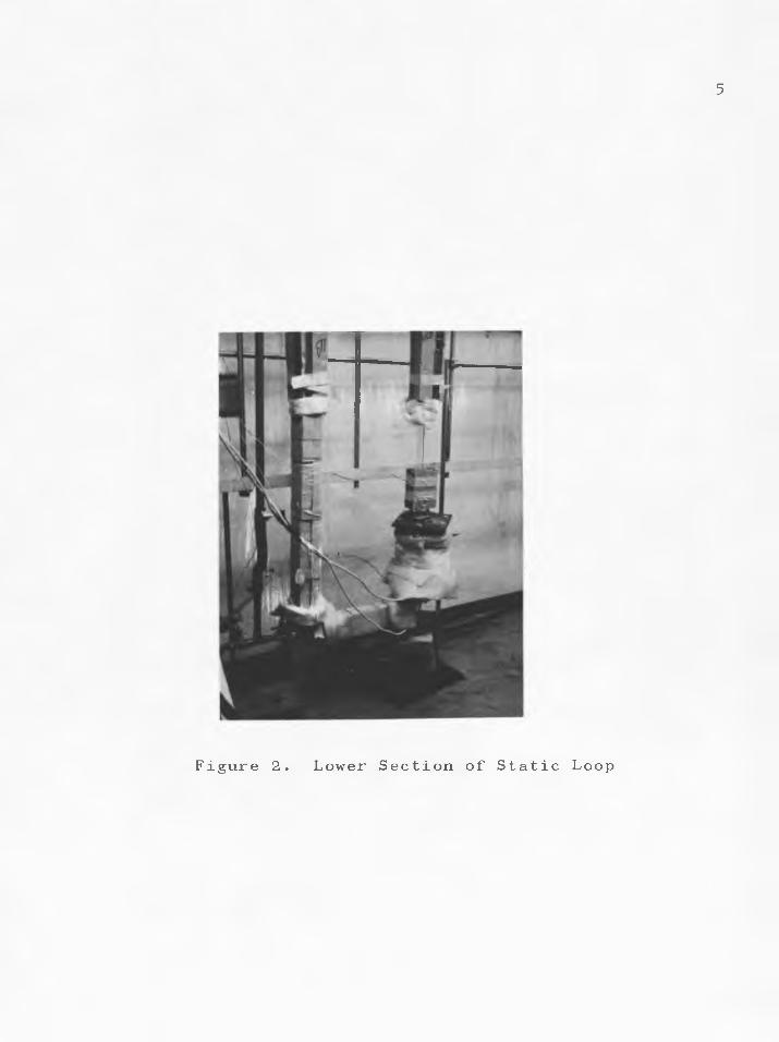
5

Figure 2. Lower Section of Static Loop

6positions: in the loop, on metal surfaces, and in the

coolant flow stream at the outlet of the heat exchanger

(Figure 3)• The thermocouples were then connected to a

multiple pole switch connected to a single channel Weston

Recorder. A rotameter and wattmeter were used to measure

fluid flow and heat input.

The instruments and the techniques of calibration

are an important preliminary of the experiment. Three

instruments were calibrated: Weston recorder, rotameters,

and thermocouples.

The Weston Recorder was calibrated with a Leeds and

Northrup voltage source. Errors were found to be less than

one half of one per cent of the full scale reading or 0.05

millivolt. A slight hysteresis was noted: readings for

increasing voltage were slightly different than for

decreasing voltage.

The rotameters were calibrated using room tempera­

ture (220C ) tap water. The tap water was turned on to the

desired flow setting and the water was run into a 1000

milliliter volumetric flask and the time to fill was noted.

The filling of the flask was calibrated with less than one

per cent error using 22°C water.

Thermocouples were calibrated using 24°C as a

reference temperature. Readings from coated and uncoated

thermocouples were taken using the rotating loop partially

disassembled. The instrument measuring thermocouple

Figure 3• Overall Rotating Loop

8voltages was a Weston recorder« The calibration curves

were then determined.

The following sequential procedure was used for all

experimental runs.

1 . The loop was filled with water.

2 . If a loop was to be rotated^ the desired angular

velocity had to be attained.

3 . The coolant flow was turned on to a maximum

measureable amount.

4. Electrical power to the heater was turned to the

desired value read on a wattmeter.

5. The temperature and flow were recorded up to and at

steady state.

6 . The coolant flow was lessened to the nearest

calibrated rate of the rotameter.

7 o In a stepwise procedure 9 each new flow was main­

tained and recorded with the steady state

temperature; then the flow was lessened.

8 . When the loop temperature became too high or the

wattmeter indicated electrical breakdown9 the run

was terminated.

In the procedures listed9 the range of electrical

power to the heater went from 200 to 700 watts.

Steady state temperatures were attained at a

minimum of two to three minutes. Two to four sets of

measurements were taken at one minute intervals.

Most coolant flow settings followed the pattern of

1509 125? 100 9 80 9 609 509 40 9 30. The number of settings

attained varied from three to eight for high to low watt-

ages respectively.

THEORY

Considerations

The theory of convection perpendicular to rotation

is developed from the approach of a heat balance and a

pressure balance. The purpose of this theory is to set up

equations that apply to the particular experiment and solve

for the mass flow. Whether Coriolis forces affect fluid

flow will be determined from the mass flow data of the

rotating loop.

The following assumptions were made to simplify the

mathematics:

1 . Steady state mass flow

2 . Constant enthalpy profile of fluid but no back-

mixing

3 * Steady state temperature of surroundings

4. Constant specific heat fluid

5* Constant pressure in two phase

6 . Slip ratio dependent on quality and direction of

flow

7. Heat transfer constant around loop perimeter

8 . Single phase density a linear function of tempera­

ture

10

11An important concept of the heat balance theory is

that of the heat transfer. The mass flow and heat reten­

tion are inversely proportional to a constant. For the

entire perimeter 9 this is approximately true. The varia­

tion is minimized by insulation.

A most important assumption of the pressure balance

theory is that constant pressure exists in two phase

boiling. The actual boiling pressure varies depending on

the momentum transfer 9 the acceleration gradient 9 and

buoyancy of the two phases. The maximum liquid pressure is

assumed the average pressure.

From the above assumptions 9 basic approaches of

computing mass flow are developed in this chapter. The

first approach is derived from a heat balance; while the

next approach is based on a pressure balance. In the

following chapter these approaches are applied in three

steps. The heat transfer is initially computed from

measured quantities of loop heat flow, single phase

temperature 9 and length. Single phase or two phase flow

is taken into consideration. With the heat transfer

defined, the experimental mass flow can be calculated from

a heat balance. The analytical mass flow is finally

obtained from a combined heat and pressure balance computa­

tion using the principles of fluid dynamics as well as

computed heat transfer, measured heat flow, lengths, and

angular velocity.

12

Temperature 9 Quality, Heat Equations

Derivation

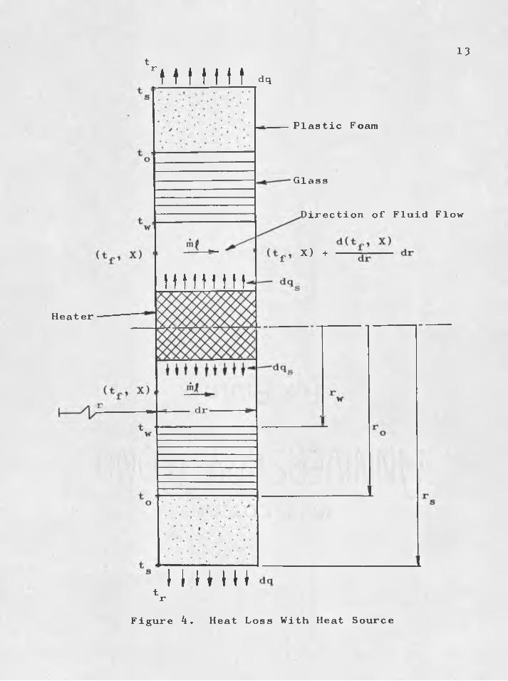
Consider an element of the rotating loop at a

uniform heat source in a fluid stream as in Figure 4. If

Q is the rate of heat input of the heat source of length (3 9

Q dr/p is the rate of heat input for a length dr. Thee

fluid flows past the heater at a mass flow m ^ « From

previous assumptions of either constant specific heat for

single phase or constant pressure for two phase9 with

quality9 X 9 the heat balances are:

Single Phase:

dq dqs - m 0c 'f£ p dr

Two Phase:

I " mzlCp d F (1 )

dq = dqs - m/ h£g g dr Q . . dX F " mJlhfs dr (2 )

l •The heat loss dq, can be calculated from the

geometry, film coefficients at the wall and surface, and

thermal conductivities » The overall heat transfer coeffi­

cient for a cylindrical geometry (Jakob and Hawkins, 1957)

is:

1u =

ln(r /r ) o wr ---=------w k wo

ln(r /r ) r ns o , w 1— ----- T -------------- + — e, -----k r hs s

+ r ' w os(3)

13tr M M M t dq

Plastic Foam

Glass

irection of Fluid Flow

X) +

H H t t t nHeater

I I H HItr

Figure 4. Heat Loss W i t h Heat Source

14where

dq = U • (2TCr dr) ° (t „ - t ) w x r (4)

Substituting (4) in (l) and (2) and solving for

t^ - t for single phase and t^ - t^ for two phase.

Single Phase:

tf *r ™ (27i:r |d)U 27rr UWTwo Phase:

^r (27lr 3 )U - m l A P9 c I 2TCr U | dr A P \ w

(5)

(6)

Solutions

The general solutions to the differential equations

(5) and (6) in simplified form are

Single Phase:

t_ = t 4- t + Const f r p e-r/AtK

(7)

Two Phase:

Cp (tr ^ tp - tb )fg m^K + Const (8 )

where K = c /2TCr U . P w

t Q Q _ QKp - XziS.F)u ~ W ~

w pand (9)

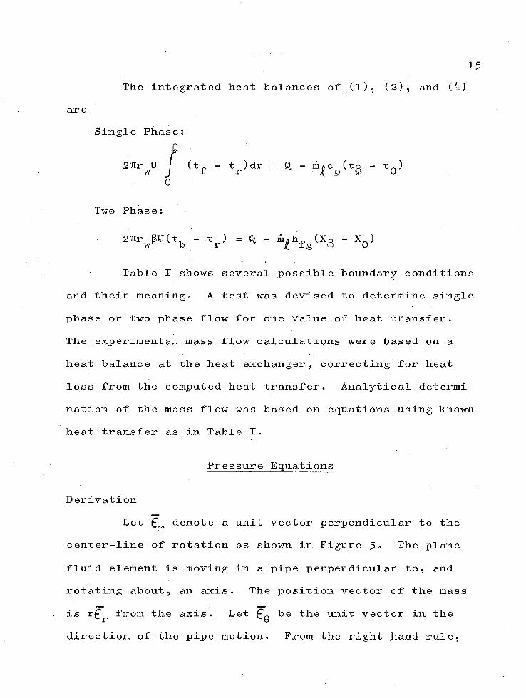
15The integrated heat balances of (l)? (2) 9 and (4)

are

Single Phases

27Tr U w0

Two Phase:

27trw |iD(tb - tr ) - q - ^ h f.g (xe - X0 )

Table X shows several possible boundary conditions

and their meaning= A test was devised to determine single

phase or two phase flow for one value of heat transfer.

The experimental mass flow calculations were based on a

heat balance at the heat exchanger 9 correcting for heat

loss from the computed heat transfer. Analytical determi­

nation of the mass flow was based on equations using known

heat transfer as in Table 1.

(t - t ) dr r Q, — m cP (t6 ” to )

Pressure Equations

Derivation

Let denote a unit vector perpendicular to the

center-line of rotation as shown in Figure 5 ° The plane

fluid element is moving in a pipe perpendicular to, and

rotating about 9 an axis. The position vector of the mass

is rf from the axis. Let be the unit vector in the

direction of the pipe motion. From the right hand rule 9

Boundary Conditions

Single Phase

Two Phase

Temperature Equations

Single Phase

Quality Equations

Two Phase

Heat Equations Integrated

Single Phase

Two Phase

t . = t at r = 0

X = at r = 0

t „ = t + t + r r tr - V

c (t + t - t ) P r p bfg 4k

Q - q 2TUr pU w*2 - tl

t + t r_____P - t

tr + S - t.

Q - q = Q - 2TTr PU(t, - t ) ^ w b r

Note: In a region outside the heat source the same ec

l6

Equations

i U n c alculated Heat Transfer

tf ~ t^ at r = 0; tf = t^ at r = (3

X - at r = 0; X = X_ at r = (3

ki

(3+ t ____P+ tP

tt1

2

Pcp (tr + tp - tb )h f g (X2 - V

Q - q = m < C p (t2 - t l )

Q - q = m ^ h f g (X2 - X^)

:s apply with t = P 0 and Q = 0.

P + dPM 1 M i +

W W W VT t t

vWall

dm

r

9

Figure 5 . Force D iagram of Fluid Flow

18the angular velocity vector LV is LJ£ The fluid mass

center is in motion relative to the pipe wall at a constant

velocity v_ in the -£ direction. The differential fluid

mass dm has a vector momentum:

d(rer )vdm = -- 7T-- dm = (-v Cr + Gu/rCg) dm

The momentum vector changes magnitude and direction,

By Newton!s Second Law9 a force vector results. dm = Q Adr

and dm =^QAdv^,

4TdF = A < dPf + drf + (£ + &) v„2(§(r)drf

- -rr < Vdm dt ' '

After division by A,

dm + vdm dt

a pressure equation results,

4TdPCr + -5^ dr€r + ( jf + ) vr2§(r ) drfr

= -pg cosGu/t dr£‘r - p U 2rdr€r - DL>J-vrar€Q

- f)v dv F r r r

The fluid element dm has an average radial velocity2v relative to the tube wall. Let d m be a fluid element of r

dm with an exact radial velocity v^ shown in Figure 6 .

Because the exact velocity v _ varies in the Qz plane ? the

Coriolis forces vary in the ©z plane. The total force on

dm is in the + Cq direction:

19

U

ActualVelocityDis t r i b u t i o n

<A

c h ui

e

Dis t r i b u t i o n (View from Top)

dm

D

Coriolis Force Current

Figure 6. Fluid Velocity and Flo w

20

dF =j / d^F =5 | d^m( 2 GVG x (-v1 £* ))c J c J z r^r

=5 2dmUv f r 0

The actual Coriolis force distribution is non-

uniform in the plane, The density is also non-uniform in

the 9z plane^ because the fluid medium conducts heat - The

resulting second order effect is a double vortex as in

Figure 6. A non-uniform force distribution acts on a non-

uniform density distribution - The velocity averaged energy

of the double vortex in dm is:

dEC = / d'2Ec = I / d2mv© 2 = I ^ Q 2 (10)

where v^ is exact and v^ is average.

Let the tangential vector of the eddy current

velocity v^ be dr f . A space-averaged current has the

dimension D _ in the 6% direction» This current traverses

a round trip distance of 2Dg in the direction of the

Coriolis forces• The space-averaged energy of the double

vortex is

( 2 U C x ( -v 1 C ) ) ° dr f z r r

=5 2dmVvr 0 (11)

where v 1 is zero near the wall» r

21

After equating the velocity and space-averaged

energies, equations (10) and (ll), an equation of v^

results:

V0 = WV ^ D g ■D (12)

The Moody friction factor (Moody^ 19^4) is related

to the Coriolis effect by the wall shear stress:

2fp — = fp

2 , 2 V r * V 6 =! f,P + 2Dgf p U v r = 4T

where v is the total fluid velocity with respect to the

wall of the pipe.

Summing the forces in the Cr direction and letting9

dP + fp -|- — + fp(>tyvrdr + (£+$.> vr 26(r)dr

+ p g cosLJt dr + p b J rdr + jQv^dv^ = 0 (13)

Solutions to the Differential Equation

The general pressure equation for a segment r^ to

r. is broken into components in Table II. The radius r is Ja loop perimeter variable. The quantities of r have dif­

ferent meanings when applied to friction and horizontal

integration. For the friction terms r. - r. is an absolute1 Jvalue and is integrated over the entire perimeter. For

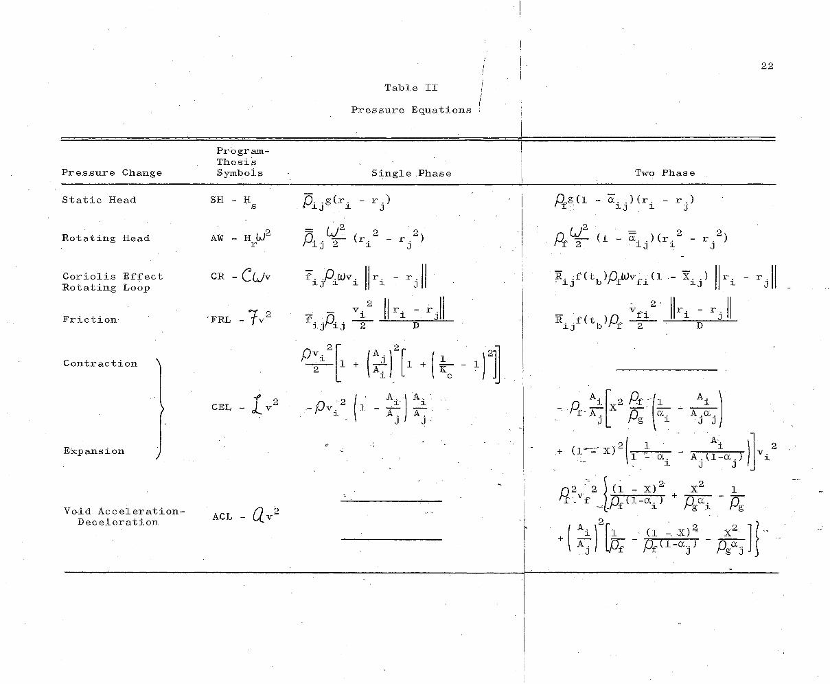
1Table II /

1Pressure Equations i

22

Program-Thesis

Pressure Change Symbols Single Phase Two Phase

Static Head SH - H ' s Pi.i -(,A - r j ) P f s (l - ai j (ri - r

Rotating Head AW - H U 2 r (ri2 - r / ) Pf^2“ (1 - E ij)(ri2 “ r j2)

Eijf(tb )pfw v fi<1 - %ij)Coriolis Effect Rotating Loop

Friction 'FRL

Contraction

A .a..J J

Expansion

2 2 ) (1Void Acceleration-

Deceleration

23integration that is parallel to the center line of rota­

tion 9 both the Coriolis effect and the static and rotating

pressure heads do hot change.

The meanings of the symbols in Table II are listed

in Tables III and IV (Lottes 9 1961) . Density is assumed a

linear function of the temperature for 20°C e t c 110°G.

Because density is linear with temperature^ the weighted

densities are solved for in terms of distance weighted

temperatures. The slip ratio is assumed a logarithmic

function of the quality only (lsben9 1957)« In calculating

weighted void fractions 9 the slip ratio is assumed a

constant average before integration.

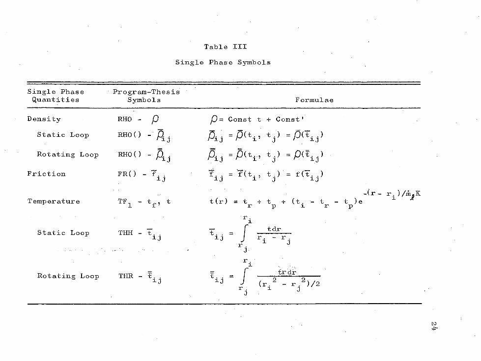
Table III

Single Phase Symbols

Single Phase Quantities

Program-ThesisSymbols Formulae

Density RHO - p P = Const t + Const 1

Static Loop RHO() - p± . Pi, =P(ti’ tj) =Paij}Rotating Loop RHO() - p ± . P±j =P(E> tj)

Friction F R O - f. . hj = ?(ti’ t)) = f(Tij)Temperature TFi - h> 1 -(r - r ) /m,K

t (r) = tr + tp + (t± - tr - tp )e

riStatic Loop THE - "t. .ij t.. = f tdr10 J ri - r.i' iRotating Loop TER -

> ,5 / tr drlj " J. «ri2 - -j2)/2J

to

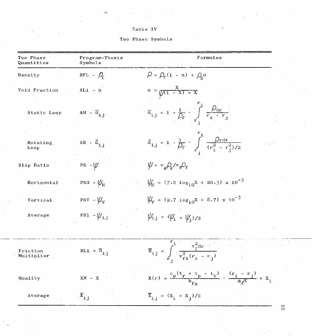
Table IV \

Two Phase Symbols

Two Phase Program-Thesis FormulaeQuantities Symbols

Density RFL - Pf p = p f d ■- oc) + D oc

Void Fraction a l i - ay / u - X) + X

Static Loop AH — GC. . ai j = 1 ~r . ? Pdr

A rJj

ri ' r j

RotatingLoop

AR - S ±Jri

— * f Pr&va ij - 1 P f J

r d(r? - r^)/2

Slip Ratio ps -y/ v gPg/vA

Horizontal f s h - % <7.2 loglG:X

cnioH%OCM

Vertical PSV - ^ v % = (2.7 loSioX + 8 .7 ) x 10-3

Average psi -y/ij = ( % " ^ j >/2

Friction RL1 - R. .Multiplier "L^

Quality XM - X

Xid

VX (r ) cp (tr - S - tb )

h g(ri - r .i)

lhJK+ X.

xij = (xi + x j )/2Average

DATA ANALYSIS

Calculating Mass Flow

Convection perpendicular to rotation is not well

understoode One method of measuring convection is by

temperature changes in a heated stream of a rotating

convective loop. The mass flow can be calculated by a heat

balance. From analysis of momentum changes and the

hydraulic head9 the mass flow can be calculated by

including heat transfer data 9 loop dimensions? and angular

velocity. A pressure effect from Coriolis forces is

included in the calculation. A comparison of the mass

flow calculated by the two methods will give an indication

of the validity of the calculation of the Coriolis pressure

effect.

In a physical system such as the rotating convec­

tive loop? a balance of enthalpy around the perimeter is

necessary and sufficient to provide the heat balance to

solve for the mass flow. An important factor is the heat

loss in the loop. The product of the mass flow and heat

retention is a useful function to evaluate the heat loss

with distance and power input. The product can be averaged

for the entire perimeter of the loop. Once its value is

known? the mass flow and heat retention can be solved for.

26

27In calculating the mass flow by fluid dynamics9 a

temperature-mass flow balance must be attained. First the

following data must be known: the temperature change with

distance known from the heat transfer 9 the loop dimensions 9

heat flow9 and angular velocity. The temperature equations

are based on the calculated heat transfer equations of

Table I, while the mass flow is calculated from pressure

equations based on Table II. In order to solve for the

balanced temperature and mass flow9 an initial temperature

and mass flow are assumed. In the first step of the

computation9 the temperature calculations proceed down­

stream to the starting point. The new temperature is the

calculated starting point temperature after one circuit.

A new mass flow is also calculated from pressure changes

taking downstream temperatures and qualities into account.

The new temperature and mass flow are compared to the old.

If there is a difference between the old and new values 9

the computation process is repeated with new starting point

temperature and mass flow values substituted. When the old

and new values of temperature and mass flow are minimal9

the fluid dynamic calculation is complete.

Once the mass flow is calculated by the two methods

described above 9 comparisons are made and conclusions are

dr awn.

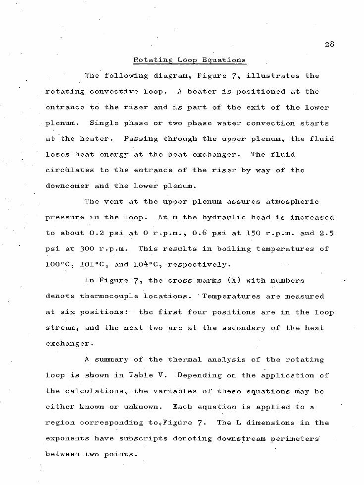
28Rotating Loop Equations

The following diagram. Figure 7 , illustrates the

rotating convective loop« A heater is positioned at the

entrance to the riser and is part of the exit of the lower

plenum. Single phase or two phase water convection starts

at the heater. Passing through the upper plenum, the fluid

loses heat energy at the heat exchanger. The fluid

circulates to the entrance of the riser by way of the

downcomer and the lower plenum.

The vent at the upper plenum assures atmospheric

pressure in the loop. At m the hydraulic head is increased

to about 0.2 psi at 0 r.p.m., 0.6 psi at 1$0 r.p.m. and 2.5

psi at 300 r.p.m. This results in boiling temperatures of

100 °G, 101°C, and 104°C, respectively.

In Figure 7? the cross marks (X) with numbers

denote thermocouple locations. Temperatures are measured

at six positions: the first four positions are in the loop

stream, and the next two are at the secondary of the heat

exchanger.

A summary of the thermal analysis of the rotating

loop is shown in Table V. Depending on the application of

the calculations, the variables of these equations may be

either known or unknown. Each equation is applied to a

region corresponding to^Figure 7 * The L dimensions in the

exponents have subscripts denoting downstream perimeters

between two points.

Two Phase

--- QHeater . l6 cm

Figure 7• Diagram of Rotating LooptoxO

Table V

Thermal Analysis of Rotating Loop

Region Equations

Single Phase

1 to m-L /m-K

t = t + t + (t - t - t ) e mm r p 1 r p

m to 2-b /mxK

*2 = + (tm -

2 to I-L /muK

*1 = *r + (t2 ' tr )e

I to 0 t0 = *1 - q ' / ^ c p

0 to 3-L /m K

*3 = *r + (t0 - tr )e

3 to 4-L ^/m^K

*4 = tr + <t3 - tr )e

4 to l = + (t4 " tr )e

t + t + (t,, - t - t ) er p 1 r p"Lib1/lil(K

. , , ^ + S - *1Lib1 = m(K ln t + t -1 r p b

V = (Llm - L lb )cp (tr + S ' tb1 )/(hfgXm )

= Lmb2cp (tb 2 - tr )/(hfgXm )

mb2 = (Llm - Llb1 )(tr + tp “ tb2 )/(tb2 ' * r }

t2 = t + r-Lb02/AiK

tr )e

single phaseVjOO

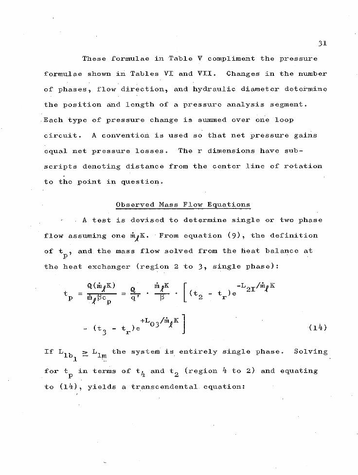
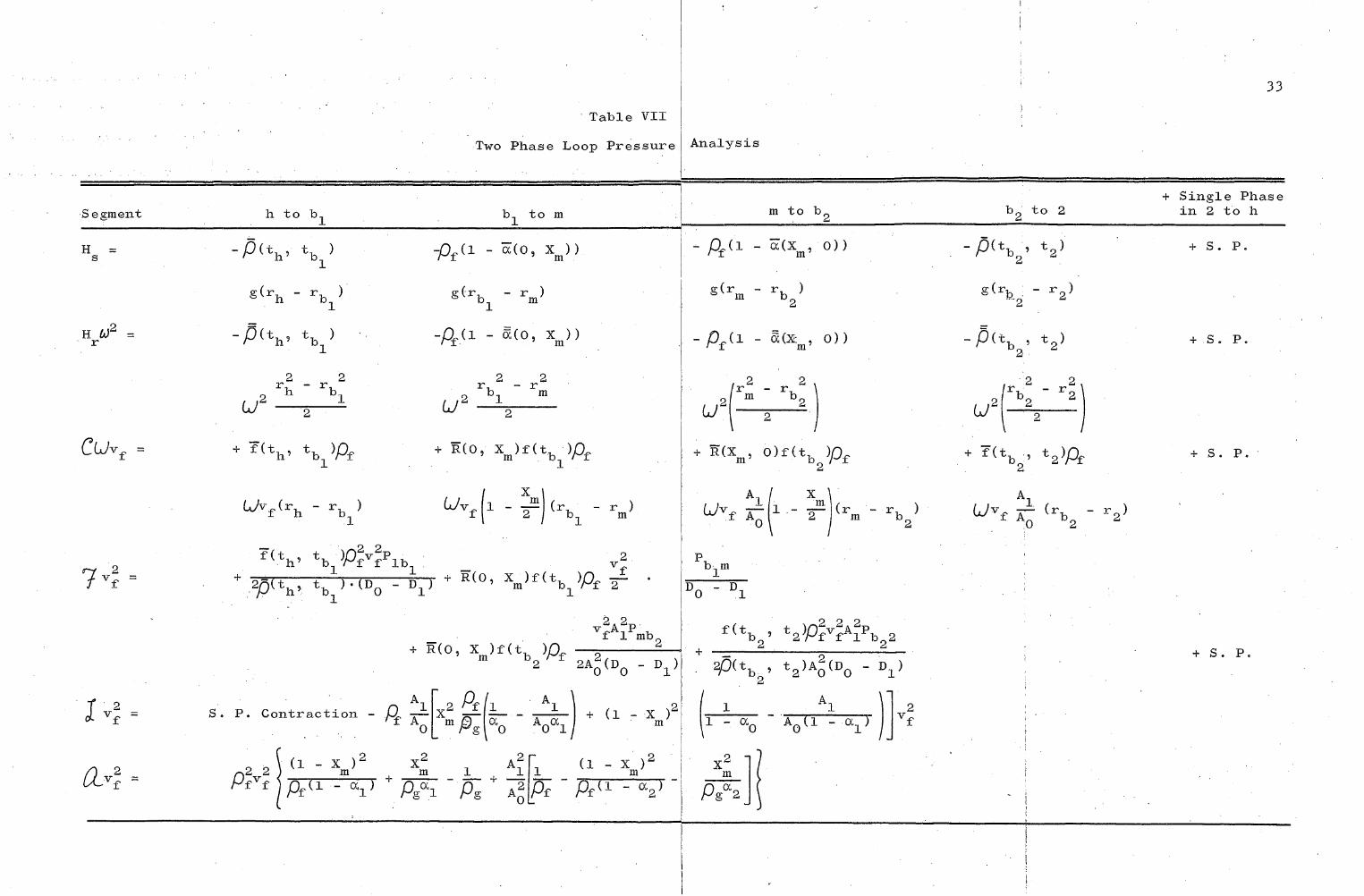
31These formulae in Table V compliment the pressure

formulae shown in Tables VI and VII„ Changes in the number

of phases 9 flow direction9 and hydraulic diameter determine

the position and length of a pressure analysis segment.

Each type of pressure change is summed over one loop

circuit. A convention is used so that net pressure gains

equal net pressure losses. The r dimensions have sub­

scripts denoting distance from the center line of rotation

to the point in question.

Observed Mass Flow Equations

A test is devised to determine single or two phase

flow assuming one m^K. From equation (9)9 the definition

of t 9 and the mass flow solved from the heat balance at Pthe heat exchanger (region 2 to 3 9 single phase):

Q(m^K) « mjK~T~ (t2 " tr )e

-L 2I/A/ K

- (t, - t )e+L° 3 ^ K3 r(l4)

If > L the system is entirely single phase. Solving1 ™

for t in terms of tr and t (region 4 to 2) and equating P 2to (l4)9 yields a transcendental equation:

Table VI

Single Phase Loop Pressure Analysis

Segment h to m m to 2 3 to 4

H = s - P (tH ’ - rm ) - P (tm ’ - r 2 ) + P ( t 3 , t4 )g(r4 - rj)

2 2 2 2 2 2HrU 2 = - p (th , t j w 2 - P < V * 2 )m2 !2L^ + P ( t 3 , t4 ) ^ J L L - 1

II • (H

O

+ f<th , tm )Wp fvf (rh -A

rm ) + f(tm ’ t2)UPt:vf 5 7 (rm " r 2 )0+ f(t3 , V ^ P f V f <r4 - r3)

'Y 2 _ . T ( V f (tm , R-- P) 5f: three elbows __+ TT=r

X

2P u i> V lDo - “ l'

2* Pt —

15f: one tee

A ? \ /, )2 1l— <

+ i ! 1 + ( * : ‘ l) 1 -~o\

A.

Segment

7

ICL =

Two Phase Loop Pressure

Table VII

h to b,, b1 to m

H = s - P (th ’ tb1 ) "Pf(1s(rh - rb, >1

g(^

H =r .- ^ wrh - rb.2

H

U 2---2-^ U 2 ■

n> ? II + F(th ’ tb1 }Pf + R (0

r 2 - r2 b_, m

- rb1 )

f(th> S ' ^ P ^ i b ,

u. 1 - (% " r™)r -r + R<0, xm)f(t )pf -j

vfAlPmb.+ K<0’ -ZST-T)O' 0A,

S . P. Contraction - fX1 Ao

2 A; 1 Ab 1 + (1 - X )2 mi a i '

[ m P g 1% ‘L Aoaij 1 - ( 1 - )/

'ff 1Ara - ap ■ pK<x pg A u - xm >'Pf Pf a2

33

Analysis

m to b. bg to 2

- P f (i - E(xm , o)) - p aV t2>g(rm - rb2) g(rb 2: - r2)

- Pfd - S(sm , 0 )) -p(tb , t2)2 ■

/r2 - r 2 \ fr.2 - r2u2 m „ b2 U2 b2 2

Q

+ R(Xm , 0 ) f ( t ^ p f

A. / X >Al1 - f <r- ' - V+ t2)pf

U v f (rb2 " r 2 )

b^m

Do - Di

f(tb2> t2)PMA?Pb22t2)A0 (D0 - Dl>2

-2 1

P s S

+ Single Phase in 2 to h

+ S. P.

+ S. P,

+ S . P.

+ S . P,

34

+L

V cT(t2-tr )e )e-L^ ^ K4 r

n r v T F " ie -1f -L / ^ K +L /m,K(t „-t )e 21 * -(t_-t )e 03 ^ -1ur\UM

(15)

If c L- m the system is partially two phase.

Equating m^K in the boiling regions (b^ to m) and (m to b^)

and solving for the single phase downstream lengths L1

and 2 :

(L - 6,Kin / t tE '. t;)(tr + .tp " S ’ r p b ^

a m2 " ,i,/ Kln - tr >(tb - tr ) = (16)

Equation (l6 ) combined with equation (l4) yields a

transcendental equation in m^K for two phase«

Once the transcendental equations of m^K are

solved 9 the mass flow, heat retention, maximum temperature,

and maximum quality can be determined by algebraic manipula­

tion of the above equations.

Analytical Equations

Analytical calculations involve the same tempera­

ture formulae as are shown in Table V . In all cases of

single phase or two phase flow, the calculations proceed

downstream from an assumed temperature at t^. The same

35temperature must be calculated after one circuit » In

general9

ti = T(™()» ti )

However 9 the presence of bubbles in the riser affects the

mass flow.

The formulae that follow govern the number of

phases . Five cases are possible «> but only two cases were

experimentally feasible as in Tables VI and VII.

Case I . Single Phase Flow Around the Entire Loop.

The length of heater necessary to bring about boiling must

be greater than the heater's actual length:

L1V ™eKln

Case II . Two Phase Flow in the Riser Only. The

length of two phase flow downstream of m is less than the

distance from m to 2 :

LmT32= (Llm " Llb1) ( ) ^ Lm 2

From the information on temperatures 9 qualities 9

and the lengths of two phase flow9 the velocity9 v^ 9 and

mass flow9 , are calculated.

Mass flow is the product of the fluid velocity9

density, and area at one point. The velocity is calculated

from a pressure formulation with the effect of Coriolis

36forces considered« Density is a function of temperature or

quality9 while the area is assumed independent of tempera­

ture o The mass flow is at steady state9 the path being

constrained within a rotating convective loop„

From the sign convention 9

Pressure losses = Pressure gains

After summing pressure changes around the loop:

Static loop x+7+a> = Hs

Rotating loop (J +

(17)

(18)

Formulating the mass flow from its definition, (17)? and

(18),

71 (D^ - DStatic loop x

Rotating loop

i> x l /J+T3 + (l

2(x+r? +a.)In summary^ all five possible cases of analysis are

functions of the independent variables t^ and m ^ :

rhj| = M(mj| t^) <>

The temperature and mass flow formulations are

boundary conditions for each other. Two subroutines are

necessary in a computer program solution:

SUBROUTINE TEMP = T(t^, )

SUBROUTINE PRES mj = M(ih| , t^).

When t - . OOOO51' < t < t 1 +± JL — ± — ±

and mj- - .00005mj

.00005t^

.00005m|

the mass flows and temperatures are simultaneously

balanced. Theoretical values are to be- compared to

experimental values.

RESULTS AND CONCLUSIONS

Mass Flow-Heat Retention Data

The product of the mass flow and heat retention is

calculated from experimental data. This product is the

distance at which the stream-room temperature difference

changes hy a factor of e , A plot of the mass flow (linear

scale) versus the product of the mass flow and heat

retention (log scale) is shown in Figure 8 , The straight

line represents almost all of the rotating loop data.

The heat retention values of the rotating loop are

low. This is caused by two effects: a high film coeffi­

cient of heat transfer of the insulation-air interface at

high angular velocity9 and a small hydraulic diameter at

the heater causing high friction and low mass flow. High

values of heat loss justify the analysis of temperaturei ' .

with distance,

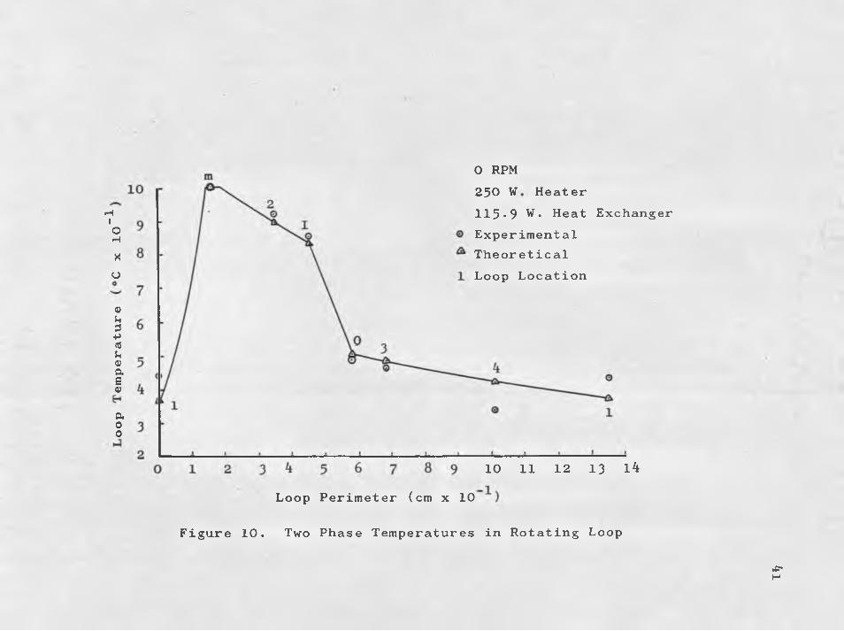
Temperature Data

Theoretical temperatures are compared to measured

temperatures of the rotating loop stream. Two cases are

shown: one with temperatures below boiling (Figure 9) and

the other with maximum temperature at boiling (Figure 10),

The total perimeter of the loop is 135 centimeters;

consequently% the temperatures at 0 and 135 centimeters

38

Mass

Flo

w, m, (G

m/se

c)© Measured Values300 r.p.m. 300 w . Heater

8 .9 1.0 3-0 4.0 5.0 6.0 7.0 8.0

Mass Flow Heat Retention Product, m«K (cm x 10 )

Figure 8. Rotating Loop Heat Transfer

vi\D

300 RPM300 W . Heater49.1 W . Heat Exchanger

© ExperimentalTheoretical

1 Loop Location

10 11 12 13 l4Loop Perimeter (cm x 10 )

Figure 9• Single Phase Temperatures in Rotating Loop

rHIoiHXo

0)ud-p(0k0)aE<yaoo

0 RPM250 W Heat er115*9 W . Heat ExchangerExperimentalTheoreticalLoop Location

10 11 12 13 14Loop Perimeter (cm x 10

Figure 10. Two Phase Temperatures in Rotating Loop

►s-H

42

are the same« The numbers and letters denote the loop

location in Figure 7» The circled points indicate the

calculated mass flow from measured data9 while the

triangles indicate the calculated mass flow from a pressure

balancec A line connects the theoretical data points. In

the single phase portions of the graphs the curves are

exponential. The two phase portion is represented by a

horizontal line at boiling temperature. A straight line

temperature distribution is assumed through the heat

exchanger.

The angular velocity of the system is an important

factor. Note the relatively high temperatures upstream of

the heat exchanger for the 0 rpp.m. case. At m the system

is two phase starting 0.3 cm upstream and ending 3 ° 0 cm

downstream. In the 0 r.p.m. case most of the heat is

dissipated through the heat exchanger, whereas at 300

r.p.m. most of the heat is dissipated through the loop.

The downstream temperatures of the heat exchanger are on

the average 10°G higher than the corresponding temperatures

for 0 r.p.m.

The close relationship between the data-analyzed

temperatures and the experimental temperature is a good

indication of the validity of the theoretical analysis.

43

Mass Flow Data

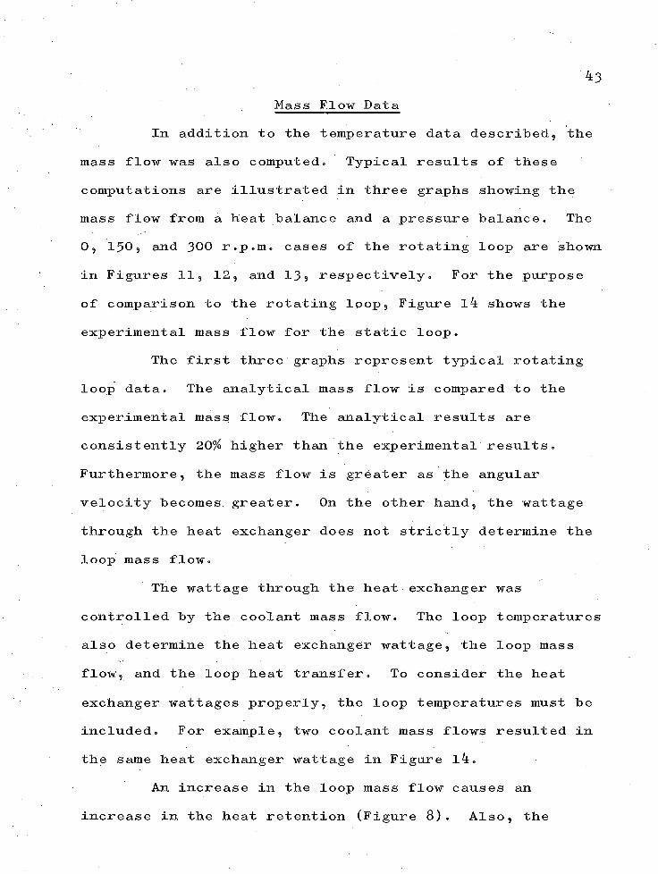
In addition to the temperature data described9 the

mass flow was also computed. Typical results of these

computations are illustrated in three graphs showing the

mass flow from a heat balance and a pressure balance. The

0 9 150 9 and 300 r.p.m. cases of the rotating loop are shown

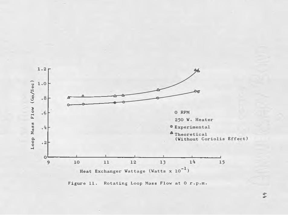
in Figures 119 12 9 and 13 9 respectively. For the purpose

of comparison to the rotating loop 9 Figure l4 shows the

experimental mass flow for the static loop.

The first three graphs represent typical rotating

loop data. The analytical mass flow is compared to the

experimental mass flow. The analytical results are

consistently 20% higher than the experimental results.

Furthermore 9 the mass flow is greater as the angular

velocity becomes greater. On the other hand9 the wattage

through the heat exchanger does not strictly determine the

loop mass flow.

The wattage through the heat exchanger was

controlled by the coolant mass flow. The loop temperatures

also determine the heat exchanger wattage 9 the loop mass

flow9 and the loop heat transfer. To consider the heat

exchanger wattages properly9 the loop temperatures must be

included. For example 9 two coolant mass flows resulted in

the same heat exchanger wattage in Figure l4.

An increase in the loop mass flow causes an

increase in the heat retention (Figure 8). Also 9 the

Loop

Mas

s Fl

ow (G

m/Se

c)

Figure 11. Rotating Loop Mass Flow at 0 r.p.m.

4

168 172 176 180 184 188 192Heat Exchanger Wattage (Watts)

►e*vnFigure 12. Rotating Loop Mass Flow at 150 r.p.m.

Q 9

Loop

Mas

s Fl

ow (G

m/Se

c)

c

300 RPM300 W . Heater

9 Experimental& Theoretical

(Without Coriolis Effect)

Heat Exchanger Wattage (Watts)

Figure 13* Rotating Loop Mass Flow at 300 r.p.m.

#*

Loop

Mas

s Fl

ow (G

m/Se

c)

14

12

10 -

8 -

48

300 W. Heater°Calculated Values

_i__________ i__________ i i i i12 16 20 24 28 32

Heat Exchanger Wattage (Watts x 10 )

Figure l4. Static Loop Mass Flow►S'-sj

48minimum loop temperature increases and the maximum loop

temperature decreases. The maximum temperature decrease in

the region of most heat loss causes the overall heat

transfer coefficient to decrease. If the minimum tempera­

ture increase is large enough9 the loop heat loss increases

for increasing mass flow as in Figure 12. If the minimum

temperature increase is not large enough9 the loop heat

loss decreases for Increasing mass flow9 as in Figure 11

and Figure 13.

Comparison of the mass flows of the static and

rotating loop shows that the static mass flow of the large

loop is several times that of the small rotating loop at

300 r.p.m. This apparent discrepancy is due to the differ­

ence of the hydraulic diameter at the heater. The static

loop heater had unrestricted heat transfer causing optimum

conditions for mass flow. In contrast 9 the hydraulic

diameter at the rotating loop heater was 0 .l6 centimeters

causing non-optimum mass flow conditions.

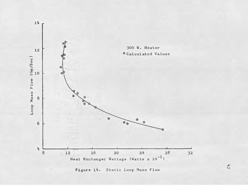
The Coriolis Effect

The non-optimum mass flow is affected by the

Coriolis forces, yet the results show that the Coriolis

effect on mass flow can be neglected.

In single phase the pressure changes from rota­

tional height and friction are about twenty times as large

as the diminishing effect from Coriolis forces. Figure 15

Loop

Mas

s Fl

ow (Gm/

Sec) 300 RPM

300 W. Heater0 Experimental^ Theoretical

(With Coriolis Effect)

Heat Exchanger Wattage (Watts)

Figure 13* Rotating Loop Mass Flow with Coriolis Effect

illustrates the Coriolis effect as 5% of the mass flow for

single phase.

When two phase flow occurs9 the pressure change

from Coriolis forces is of about the same magnitude as that

for single phase. The pressure changes from rotational

height and friction become one hundred times as large as

the Coriolis effect because a small portion of the riser

is two phase. The density of two phase steam is much less

than that of water, and the pressure change of rotational

height increases by a factor of at least ten. The increasing

effects of friction and rotational height in two phase flow

cause the Coriolis forces to affect the mass flow by less

than one per cent.

50

Errors

An estimated magnitude of error is in parentheses.

Instrumental Errors

1. Iron-constantan thermocouples were commercial

grade. Noise from slip rings added to error (2%).

2. Good quality wattmeter was used. Resistance from

slip rings and circuit added to error (1%) .

Rotameter was accurately calibrated. Rotating

seals cause flow oscillation. The average flow

was taken (2%)=

3 •

51Other Experimental Errors

1 o Backmixing and conduction were localized at the

entrance to the heater <, Calculations indicated

one-third of the heat backmixed at t^. Temperature

t was not included in experimental calculations, iTemperature t^ was extrapolated from t^.

2 o Phase separation and steam escape through the vent

in the upper plenum gave two phase heat balances

at the heat exchanger. The mass flows computed

were of single phase. These data were neglected.

Theoretical Errors

1 o The specific heat of water was assumed constant

for single phase. The specific heat varies 1%

from 20°C to 110*0 (l%).

2 . Two phase boiling was assumed constant pressure.

The two phase temperature is off 3% at the region

of maximum temperature quality (3% ) °

3• The product of the mass flow and heat retention is

constant around the entire perimeter of the

rotating loop. The downstream variation of the

film coefficients with the magnitude of the heat

transfer determines the error. The maximum

possible error of this assumption is 7% for 300

r.p.m. and 300 watts (7% ) °

524 o Other assumptions of the pressure equation are a

source of error. The assumptions of a constant

temperature profile and steady state effect amount

to 7% error (7%)«

The combined effect of all the errors 9 e^, is

formed from the product

1 - eT = (! - eTC^ ° ^ e¥M^ ’ f1 “ eRM^ ’ ^ eCp^

(1 “ ep ) * (1 ~ eHT) ? (1 - eBE)

1 - eT = (.98)(.99)(.98)(.99)(-93)(-93)(.93) = .79

The combined error is 21% between theoretical and

actual mass flow for the best data.

Conclusions

The effect of Coriolis forces on the mass flow of a

rotating loop can be neglected if the analytical computa­

tion of the mass flow is based on the Bernoulli Equation.

The effect of gravity can also be neglected if the rota­

tional acceleration is in excess of 5 g f s . However 9 the

pressures derived from rotation about a center-line must

be included. The magnitude of the Coriolis force affects

5% of the mass flow in single phase and less than 1% of the

mass flow in two phase.

RECOMMENDATIONS FOR FUTURE WORK

Fluid flow9 both single phase and two phase 9 of a

downcomer and riser in rotation can be photographed for

study o The purpose would be to give some idea of the

pattern a flow undergoes under such conditions. The bubble

size, formation rate, bubble velocity, slip ratio, fluid

path, and heater burnout could be experimentally determined

Appropriate correlations and formulations could be devised•

Two phase separation by centrifugal force could

also be studied photographically. It would be possible to

investigate the magnitude of the parameters affecting the

separation. The quality, fluid velocity, and angular

velocity would be the experimental variables. The amount

of separation and slip ratio could be experimentally

determined. , . _

The value of the heat retention constant, K, could

be evaluated experimentally and tested to theory. It could

be determined whether the concept of heat retention is an

adequate description of all possible cases. As a variable,

the heat retention could be studied in non-isothermal flow,

phase separated flow, temperature dependent flow, and

position dependent flow. Thus K could be evaluated for

compatibility of theory and experiment.

53

54The direct measurement of mass flow in a rotating

loop could be possible- A flow meter that is independent

of temperature gradients 9 fluid conductivity 9 and the

forces of gravity and rotation has been developed by

Satchell (196$)- The operation of the flow meter was based

on Faraday1s Law of Electrolysis: measurement of the mass

flow of injected ions in an ionic fluid - A comparison

could be made between the mass flows obtained by a heat

balance 3 pressure balance? and direct measurement -

APPENDIX

Derivation of Coriolis Force Pressure Loss

The change of pressure is

" X

P ve drdPc = f 2 D

Single Phases

v_ = 4Wv from equation (12) © r ©

^QlVl " P vr = constant for constant area 2

Let: 9 PVo" . 2D9W ~ P U v r

j f p u vrdr = fu j pvrdr = yTherefore: (r^ - r^)

Two Phase:

If: P = p^(l - OC.) , neglecting gas mass

Let : v 029 = 4aAr0rD9 = ^ (I^I)vfrD9 and - ^ = 1

1-Xwhere VQr = Vfr "or dow quality steam

single phase velocity in the direction

55

56

Then» ZXpx/ -^2 < r a )Tf1-dr

1 VQ2 —Let: / -2_ (l-X)dr = R(l-X) (r1-r())/r0 V09

Therefore : A P c = (l-X) (r^-r^)

Steam Bubbles and Fluid Currents Influenced by Coriolis Forces

Steam bubbles formed at the heater in rotation are

under the influence of Coriolis forces in the C_ direction =9Since the bubbles are less dense than the liquid9 Coriolis

forces buoy the bubbles in the opposite direction. The

terminal velocity of the bubbles can be calculated using

Stokes1 Law and Newton?s Second Law.

The resisting force of friction by Stokes 1 Law is

6,vRbvb.( •

The viscosity of the fluid is 9 the radius of the

bubble 9 9 and the relative velocity of the bubble to the

liquid, vb^ .

The Coriolis force experienced by a bubble is the

product of mass times acceleration:

- | ERbPb ' 2Wvbr

57The density difference of the steam and water is ~Pi0 9 andthe velocity of the bubble relative to the wall of the pipe

in the £ direction is v_ ,^r hr.The terminal velocity, vb^ 9 can be found by setting

the resisting force of friction equal to the Coriolis

force:

6,l|1RbvbJ = - I

4 P i ^ 'b br p2 9 V b

As an example, if:

= 0.05 cm, P b = 1 gm/cm'

vbr = 1 cm/sec, p, = 2.84 x 10 poise

iij = 31 • 4 rad/sec or 300 RPM, for 100°C water,

then

12.3 cm/sec

If the Coriolis effect causes eddy currents the

size of one-half the hydraulic diameter of the pipe,

Dq = .635 cm.

58

The fluid velocity in the Cg direction is

vQ = ~ \ J = "\/4 x 31.4 x 1 x .635

Vq = + 8.9 cm/sec

The terminal velocity of the bubble relative to the

wall of the pipe is:

rhl + V9 = ‘ 12-3 + 8"9 3.4 cm/sec.

GLOSSARY

m

Symbols

Area

Void acceleration factor

Specific heat of a substance at constant pressure

Energy of Coriolis effect

Force in an inertial system

Force of Coriolis effect

Loop friction factor

Moody friction factor

Acceleration due to gravity

Film coefficient of heat transfer

Enthalpy of boiling

Static height factor

Rotating height factor

Thermal conductivity

Heat retention

Contraction-expansion factor

Downstream length from start of heater to where

boiling begins

Downstream length from top of heater to where

boiling ends

Downstream length of heat exchanger

Mass of particle

59

6om

P

Q

q'q

qs

r

R

iet

uvrv

X

a

P<$(r)

P4P

Mass flow

Pressure

Total heat rate input

Heat rate output of heat exchanger

Rate of heat loss to room

Rate of heat generated to fluid

Radius of upper plenum from rotation center-line

Radius of lower plenum from rotation center-line

Radius variable

Lottes-Flynn friction factor

Total perimeter of loop

Temperature

Overall coefficient of heat transfer

Velocity in the r direction

Velocity vector

Fluid velocity at saturation temperature 9 X = 0

Quality of two phase fluid

Void fraction

Length of uniform heat source

Dirac delta function

Unit vector in the r direction

Viscosity

Density. /Fluid density at saturation temperature, X = 0

Wall shear stress .

Slip ratio

6i

u

u

b

c

f

fgh

i,

Xo

r

s

w

z

1 ,

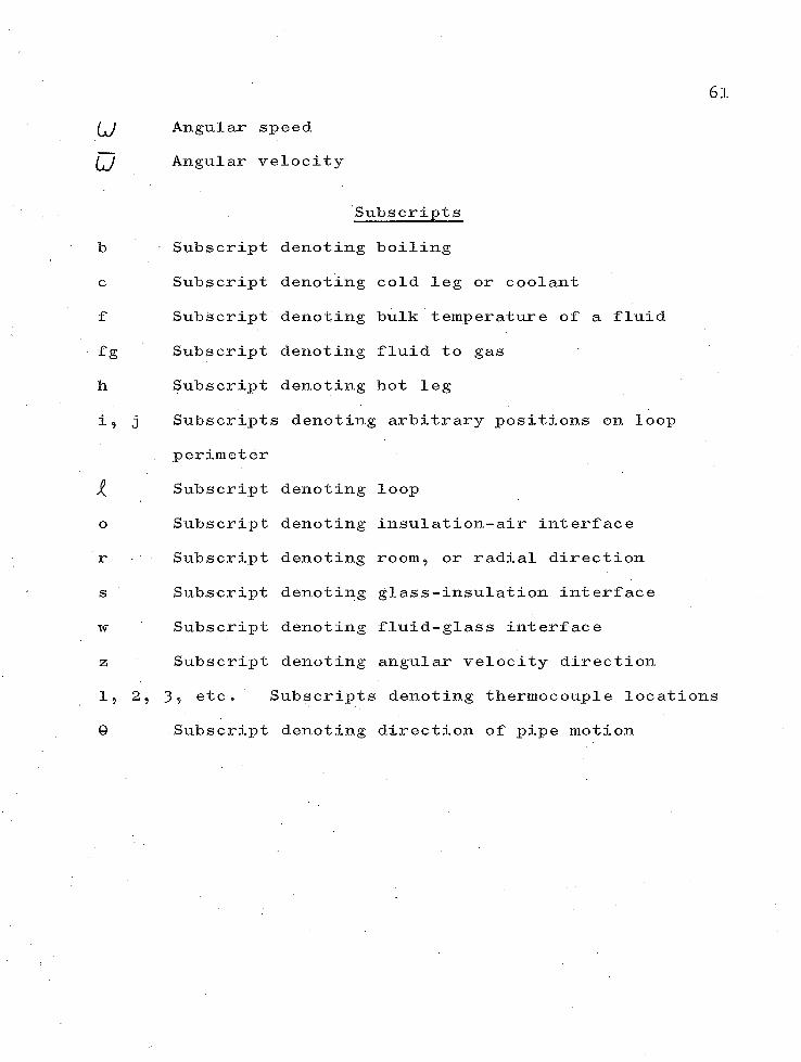
Angular speed

Angular velocity

Subscripts

Subscript denoting boiling

Subscript denoting cold leg or coolant

Subscript denoting bulk temperature of a fluid

Subscript denoting fluid to gas

Subscript denoting hot leg

j Subscripts denoting arbitrary positions on loop

perimeter

Subscript denoting loop

Subscript denoting insulation-air interface

Subscript denoting room? or radial direction

Subscript denoting glass-insulation interface

Subscript denoting fluid-glass interface

Subscript denoting angular velocity direction

2 ? 3 9 etc• Subscripts denoting thermocouple locations

Subscript denoting direction of pipe motion9

SELECTED BIBLIOGRAPHY

Blinn, H . 0. et_ aJL - 9 "Space Power Plant Study," Astro- nuclear Lab,.Westinghouse Electric Corp«,Pittsburg, NAS-5-250 »

Chang, K . S •, Akins, R. G ., Burris, L ., Jro, and Bankoff,Sc Go, nFree Convection of a Low Prandtl Number Fluid in Contact with a Uniformly Heated Vertical Plate," Argonne National Laboratory, Argonne,ANL 6835 (1964).

Christie, Clarence V 0 , Electrical Engineering, McGraw-Hill Book Coo, Inc•, New York (1952)°

Costello, Charles Po, and Adams , Jim, A d o Ch * E «J . , 9? 5?663 (1963).

Costello, Charles Po, and Tuthill, William E o , A .1« Ch•E « ,,Chemo Eng» Progress Symposium Ser. , 579 32, 189(1961)o

Elliott, David G ., "A Two-Fluid Magnetohydrodynamic Cycle for Nuclear-Electrical Power Conversion," Jet Propulsion Laboratory, California Institute of Technology, Pasadena, Technical Report N o • 32~116(1961).

El-Wakil, Mo M » , Nuclear Power Engineering, McGraw-Hill Book Coo, Inco, New York (1962)0

Isben, Ho So, A „ I »Ch . E , J » , J), I 9 136 (1957) •Jain, Kamal Co, "Self-Sustained Hydrodynamic Oscillations

in a Natural-Circulation Two-Phase-Flow Boiling Loop," Argonne National Laboratory, Argonne, ANL-7073 (1965).

Jakob, Max, and Hawkins, George, Elements of Heat Transfer, 3rd ed», John Wiley & Sons, Inc., New York (1957)»

Lottes, Paul A ., "Nuclear Reactor Heat Transfer," Argonne National Laboratory, Argonne, ANL-6469 (1961).

McAdams, William H . , Heat Transmission, 3rd ed», McGraw-Hill Book Co . , Inc . , New York (195^4) ,

62

63Merte, Herman, Jr., and Clark, J . A., J . Heat Transfer,

83, 3 , 233 (I96I) .Moody, L. F ., Trans. A.S.M.E., 66, 671-94 (1944).

Poppendick^ H » F « et al. 9 nHigh Acceleration Field HeatTransfer for Auxiliary Space Nuclear Power Systems9n Geoscience Ltd• Solena Beach9 NSA 20-407^1 (1965)0

Rohsenow^ Warren M e 9 "Heat Transfer with Boiling," in Modern Developments in Heat Transfer, Xhele,Warren, Editor, Academic Press, New York (1963)0

Rohsenow, Warren, and Choi, Harry, Heat, Mass, andMomentum Transfer, Prentice-Hall, Inc., Englewood Cliffs Tl96l).

Satchell, Max E ., "Flow Meter to Measure the Mass Flow Rate of an Ionic Fluid," Master's Thesis, The University of Arizona, Tucson (1965)0

Shames , Irving H «, , Engineering Mechanics-Dynamics , Prentice- Hall, Inc., Englewood Cliffs (i960).

Singer, Ralph M ., "A Study of Unsteady MagnetohydrodynamicFlow and Heat Transfer," Argonne National Laboratory, Argonne, ANL-6937 (1964).

Smith, C e K. , and Parkinson, R. Y . , "A 1.5 M.W.E.Thermionic Reactor Space Power System," Atomic International, Canoga Park, NSA 20-3547•

Stockett, Lawrence E ., "Measurement of Convective FluidFlow in Centrifugal Fields," Master's Thesis, The University of Arizona, Tucson (1965)*

Synge, John L ., and Griffith, Bryan A., Principles ofMechanics, 3rd ed., McGraw-Hill Book Co., Inc.,New York (1959)•

Tong, Lo So, Boiling Heat Transfer and Two-Phase Flow,John Wiley & Sons, Inc., New York (1965)°

Ulrich, A . J ., and Carter, Informal Memorandum(unpublished), Argonne National Laboratory,Argonne (1963).