Experimental study of fluctuationsin two out-of-equilibrium systems

using optical traps

Juan Ruben Gomez-Solano

Research Internship ReportMaster 2 Sciences de la Matiere

Supervisors: Sergio Ciliberto and Artyom Petrosyan

Laboratoire de PhysiqueEcole Normale Superieure de Lyon

49, allee d’Italie69364 Lyon cedex 07

France

April-July 2008.

Abstract

This work is devoted to the study of displacement fluctuations of micro-sized particlesin two different systems driven out of thermal equilibrium: an aging colloidal glass and afluid subject to a vertical temperature gradient below the onset of convection. In the firstpart we address the issue of the validity of the fluctuation dissipation theorem (FDT) andthe time evolution of viscoelastic properties during aging of aqueous suspensions of a clay(laponite RG) in a colloidal glass phase. Given the conflicting results reported in the liter-ature for different experimental techniques, our goal is to check and reconcile them usingsimultaneously passive and active microrheology techniques. For this purpose we measurethe thermal fluctuations of micro-sized brownian particles immersed in the colloidal glassand trapped by optical tweezers. We find that both microrheology techniques lead to com-patible results even at low frequencies and no violation of FDT is observed. In the secondpart, we attempt to study the influence of non-equilibrium hydrodynamic fluctuations onthe motion of a trapped particle immersed in a fluid layer (ultrapure water) subjected toa vertical temperature gradient. We estimate the contribution of non-equilibrium fluctu-ations to the power spectral density of displacement fluctuations of the particle and thefrequency range where it can be measured. Only very preliminary results are available forthis experiment.

Contents

1 FDT in an aging colloidal glass 21.1 Introduction . . . . . . . . . . . . . . . . . . . . . . . . . . . . . . . . . . . . 2

1.1.1 FDT in Laponite suspensions . . . . . . . . . . . . . . . . . . . . . . 31.2 Experimental description . . . . . . . . . . . . . . . . . . . . . . . . . . . . 5

1.2.1 Sample preparation . . . . . . . . . . . . . . . . . . . . . . . . . . . 51.2.2 Optical tweezers setup and data acquisition . . . . . . . . . . . . . . 61.2.3 Creation of multiple traps . . . . . . . . . . . . . . . . . . . . . . . . 71.2.4 Calibration of optical tweezers . . . . . . . . . . . . . . . . . . . . . 81.2.5 Microrheology techniques . . . . . . . . . . . . . . . . . . . . . . . . 9

1.3 Results . . . . . . . . . . . . . . . . . . . . . . . . . . . . . . . . . . . . . . . 111.3.1 Viscoelastic properties of the aging colloidal glass . . . . . . . . . . . 111.3.2 Properties of non-equilibrium fluctuations during aging . . . . . . . 121.3.3 Effective temperatures . . . . . . . . . . . . . . . . . . . . . . . . . . 131.3.4 Probability density functions of heat fluctuations . . . . . . . . . . . 16

1.4 Conclusion . . . . . . . . . . . . . . . . . . . . . . . . . . . . . . . . . . . . 17

2 Motion of a Brownian particle in a fluid below the onset of Rayleigh-Benard convection 182.1 Introduction . . . . . . . . . . . . . . . . . . . . . . . . . . . . . . . . . . . . 182.2 Influence of non-equilibrium fluctuations on the motion of a Brownian particle 192.3 Experimental description . . . . . . . . . . . . . . . . . . . . . . . . . . . . 22

2.3.1 Sample preparation . . . . . . . . . . . . . . . . . . . . . . . . . . . 222.3.2 Experimental setup . . . . . . . . . . . . . . . . . . . . . . . . . . . . 23

2.4 Preliminary results . . . . . . . . . . . . . . . . . . . . . . . . . . . . . . . . 252.5 Conclusion and perspectives . . . . . . . . . . . . . . . . . . . . . . . . . . . 27

Chapter 1

FDT in an aging colloidal glass

1.1 Introduction

The description of out-of-equilibrium systems is a topic of major interest in physics sincein most systems, energy or matter flows are not negligible but drive them into non-ergodicstates for which equilibrium statistical mechanics is not applicable. The typical examples ofsuch systems are slowly stirred systems and glasses. Unlike equilibrium statistical mechan-ics, whose foundations are well established since long time ago, non-equilibrium statisticalmechanics is still being developed.

One attempt to develop a statistical mechanics description of non-equilibrium slowlyevolving systems is to extend some equilibrium concepts to them, namely the so called fluc-tuation dissipation theorem (FDT). FDT relates the power spectral density of equilibriumfluctuations x of systems in contact with a thermal bath at temperature T to the responseχ to a weak external perturbation with a prefactor given by T

〈|x(ω)|2〉 =4kBT

ωIm{χ(ω)}. (1.1)

Despite of the fact that a thermodynamic temperature is not rigorously defined for non-equilibrium systems, a generalization of FDT can be done by means of an effective temper-ature Teff (ω, tw) which describes fluctuations at a time scale 1/ω. It is defined as

Teff (ω, tw) =ω〈|x(ω, tw)|2〉

4kBIm{χ(ω, tw)} , (1.2)

where tw denotes the age of the system, i.e. the waiting time since the systems left equi-librium. In general, for a non-equilibrium system either the spectral density of fluctuationsand the response function depend on tw and then violations of FDT occur when Teff (ω, tw)also depends on it.

Glasses are one of the examples of non-equilibrium systems that have been studiedextensively over the past years. They are disordered systems at microscopic length scalesformed after a quench from an ergodic phase (e.g. an ordinary liquid in equilibrium) toa non-ergodic phase (e.g. a supercooled liquid). After a quench, a glassy system relaxes

1.1 Introduction 3

Figure 1.1: Chemical structure of laponite. The disc-shaped particles form a house-of-cardsstructure in aqueous suspensions.

asymptotically to a new phase in equilibrium with the new temperature T of its surround-ings, but the time needed to reach equilibrium may be astronomical. Since the system isnon-ergodic during its relaxation, there is no invariance under time translations and thenits age tw is well defined. The slow time evolution of their physical properties (e.g. viscos-ity) is known as aging. A number of theoretical, numerical and experimental studies haveshown that two different effective temperatures are found for structural glasses [1], [2] andspin glasses [3], [4], [5] . One of them is the effective temperature associated to the fastrattling fluctuations (high frequency modes) and is equal to T . The other effective temper-ature is the one associated to the slowest structural rearrangements (low frequency modes)whose value is larger than T and decreases with time to T . Both effective temperatureshave the properties of thermodynamic temperatures in the sense that they correspond totwo different thermalization processes at different time scales [6].

1.1.1 FDT in Laponite suspensions

Regarding the existence of an effective temperature higher than the bath temperature forstructural and spin glasses, several recent works have attempted to look for violations ofFDT in another kind of non-equilibrium systems: colloidal glasses. Unlike structural orspin glasses, the formation of a colloidal glass does not require a temperature quench butthe packing of colloidal particles at a certain low concentration in water forming a glassystructure.

Aqueous suspensions of clay laponite have been studied as a prototype of colloidalglasses. Laponite is a synthetic clay formed by electrostatically charged disc-shaped par-ticles of chemical formula Na+

0.7[Si8Mg5.5Li0.3O20(OH)4]0.7− whose dimensions are 1 nm(width) and 25 nm (diameter). When laponite powder is mixed in water, the resultingsuspension undergoes a sol-gel transition in a finite time (e.g. a few hours for 3 wt %), i.e.,it turns from a viscous liquid phase (sol) into a viscoelastic solid-like phase (gel). Duringthis aging process, because of electrostatic attraction and repulsion, laponite particles forma house of cads-like structure (Fig. 1.1).

Several properties of laponite suspensions during aging have been extensively studied,such as viscoelasticity [7], translational and rotational diffusion [8] and optical susceptibility

1.2 Experimental description 4

(a) (b)

Figure 1.2: 1.2(a) Time evolution of the effective temperature of an aqueous suspensionof laponite particles (2.4 wt % concentration) during aging measured by using passive mi-crorheology [13]. Teff increases in time indicating a violation of FDT; 1.2(b) time evolutionof the effective temperature for 2.8 wt % concentration using active microrheology [12]. Un-like Fig. 1.2(b), in this case no violation of FDT is observed for any frequency and anyaging time.

[9] using techniques such as rheology and dynamic light scattering. However, the availableresults obtained so far for the issue of the validity of the FDT in this system are contra-dictory (see Fig. 1.2). Bellon et al [10] reported an effective temperature from dielectricmeasurements indicating a strong violation of FDT at low frequencies (f < 40 Hz), whereasthe same group did not observe any violations from mechanical measurements [10]. Abou etal [11] observed that the effective temperature increases in time from the value of the bathtemperature to a maximum and then it decreases to the bath temperature. Jabbari-Faroujiet al [12] used a combination of passive and active microrheology techniques (see Subsec-tion 1.2.5) without any observation of deviations of the effective temperature from the bathtemperature over several decades in frequency (1 Hz−10 kHz). Greinert et al [13] observedthat the effective temperature increases in time using a passive microrheology technique.Finally, Jabbari-Farouji et al [14] found again no violation of FDT for the frequency rangeof 1 Hz−10 kHz.

In view of the conflicting results obtained for different experimental techniques, it isnecessary to compare simultaneously at least two of them in the same colloidal glass sample.In this spirit we study the time evolution of the effective temperature and viscoelasticproperties of laponite suspensions by using simultaneously passive and active microrheologytechniques by means of optical tweezers manipulation, as explained in the following chapter.

1.2 Experimental description 5

Figure 1.3: Diagram of the sample cell used during the experiment. The diagram is not inproper scale.

1.2 Experimental description

1.2.1 Sample preparation

Physical properties of Laponite suspensions are very sensitive to the method used dur-ing their preparation [19]. Hence, an experimental protocol must be followed in order toperform reproducible measurements of their aging properties. Laponite RD, the most fre-quently studied grade and the one studied in this work, is a hygroscopic powder that mustbe handled in a controlled dry atmosphere. The powder is mixed with ultrapure water ata weight concentration of 2.8 % and pH = 10 in order to assure chemical stability of thesamples. At lower pH, the decomposition of clay particles occur. CO2 absorption by watercan modify the pH of the samples and then their aging properties. For these purposes,the preparation of the samples is done entirely within a glove box filled with circulatingnitrogen. We choose wt 2.8 % since it is known that at this concentration laponite gelationtakes place in few hours after the preparation. The suspension is vigorously stirred by amagnetic stirrer during 30 minutes. The resulting aqueous suspension is filtered througha 0.45 µm micropore filter in order to destroy large particle aggregates and obtain a re-producible initial state. The initial aging time (tw = 0) is taken at this step. Immediatelyafter filtration, a small volume fraction (0.02 ml per 50 ml of sample) of silica microspheres(diameter = 2 µm) is injected into the suspensions. Microspheres play the role of probesto study the aging of the colloidal glass, as explained further. The sample is placed in aultrasonic bath during 10 minutes to destroy small undesired bubbles that could be presentduring the optical tweezers manipulation. The suspension is introduced in a sample cellconsisting on a microscope slide and a coverslip separated by a cylindrical spacer of innerdiameter 15 mm and thickness 2 mm, as shown in Fig. 1.3. The sample cell is sealed witharaldite adhesive in order to avoid evaporation and direct contact with CO2 from air.

1.2 Experimental description 6

(a) (b)

Figure 1.4: 1.4(a) Optical tweezers setup used during the experiment: 1. Beam from aninfrared laser diode (device not shown), 2. Piezoelectric stage, 3. Microscope objective, 4.Sample cell, 5. Condenser, 6. Halogen lamp, 7. Dichroic mirror, 8. High speed camera.The paths and the directions of the trapping beam and the detection beam is are depictedin red and blue, respectively; 1.4(b) Configuration of three optical traps separated by adistance D = 9.3 × 10−6 m. The bright spots in the image correspond to three probeparticles of 2 µm diameter trapped by them.

1.2.2 Optical tweezers setup and data acquisition

Optical tweezers rely on the use of laser beams to trap dielectric particles by means of theeffect of radiation pressure [15]. When a micron-sized dielectric particle of refractive indexexceeding that of the surrounding medium, is close to a Gaussian laser beam, the refractionof light through it results in two effective forces. A gradient force is directed towards thebeam axes (the region of highest light intensity) whereas a scattering force acts in thedirection of the incident beam. If the laser beam is extremely focused (e.g. by means ofa microscope objective), there is an additional gradient force which pushes the particletowards the laser focus [16]. For sufficiently high intensity gradients, the scattering force iscompensated by the additional gradient force causing free particles to be trapped close tothe beam focus and resulting in a restoring hookean force −kx in the plane perpendicularto the beam propagation [17] (see Fig. 1.3).

The present experiment is performed in a typical optical tweezers system (Fig. 1.4(a))at room temperature (22± 1◦ C). It consists on a Nd:YAG DPSS 1 laser (Laser Quantumλ = 1064 nm) whose beam is strongly focused by a microscope oil-immersion objective(×63, NA = 1.4). Matching optics between the laser source and the objective are neededin order to direct and produce a collimated laser beam that overfills the objective entrance.The sample cell is placed on a piezoelectric stage (NanoMax-TS MAX313/M) in order to

1Diode pumped solid state

1.2 Experimental description 7

have mechanical control in three dimensions of nanometric accuracy during the trappingprocess. The sample cell is placed with the glass plate at the top and the coverslip at thebottom in such a way that the focus of the laser beam is located 20 µm above the coverslipinner surface (see Fig. 1.3). The whole system is mounted on an optical table in order toget rid of low frequency mechanical noise.

The light source used for detection is a halogen lamp whose beam is focused in thesample by a condenser lens. The halogen light passes through the sample and then theresulting intensity contrast signal is detected by a high speed camera (Mikrotron MC1310)after emerging from the microscope objective. Once probe particles are trapped properly,images with a resolution of 240×80 pixels are recorded at a sampling rate of 200 frames persecond during 50 seconds and saved in AVI format every 97 seconds (i.e. 10000 images perAVI file) for further data processing. Hence, the aging time of the system tw is measuredin multiples of 97 s while the smallest measurable time scale (the time elapsed betweensuccessive positions of the probe) corresponds to 5 ms and the highest accessible frequencyis 100 Hz. The calculation of the baricenter position of the trapped bead on the x − yplane (perpendicular to the laser beam propagation) is done by means of a MATLABimage processing program. Then, we obtain a time series (x(t), y(t)) for each coordinateat each waiting time tw. In the following, x defines the direction along which the positionof the optical trap is oscillated in time, while y corresponds the orthogonal direction. Forsimplicity, all our calculations rely on x(t) coordinates only.

1.2.3 Creation of multiple traps

Multiple probe particles are needed to be trapped within the same sample in order toperform simultaneously passive and active microrheology measurements. Since two trappedparticles are needed for each technique, as explained in Subsection 1.2.5, at least threedifferent optical traps must be created simultaneously, as shown in Fig. 1.4(b). For passivemeasurements, two traps of different stiffness and fixed positions are needed. We label theweakest trap as ’3’ while the strongest one as ’2’. For active measurements, one needs onetrap in a fixed position in order to measure the power spectral density of displacementfluctuations. For convenience, we choose trap ’2’ for such purpose. In addition, one needsan oscillating trap in order to measure the response of the probe to an external forcing. Thistrap is labeled as ’1’. The separation distance between adjacent traps is D = 9.3 × 10−6

m, which is sufficiently large to avoid correlations between their motions.The creation of three optical traps on the x− y plane is implemented by means of two

coupled acousto-optic deflectors (AOD). A high radio frequency voltage signal is sent froma signal generator to the AOD. Sound waves are created in the crystal inside the AOD,forming a Bragg diffraction grating which efficiently deflects the incident laser diode beam.The deflection angle of the output beam (the first order diffracted spot) is proportional tothe high frequency input signal. By varying the frequency of the signal generator, the angleof the output laser beam is adjusted. By coupling orthogonally in series both AOD, onecan control the angle of the output beam in 2D. In order to create three traps, the laserbeam scans three different positions along the y direction. The visitation frequency for eachposition must be large enough in order to avoid the diffusive motion of the particle through

1.2 Experimental description 8

10−1

100

101

102

10−19

10−18

10−17

10−16

f (Hz)

Sx(f)

(m2 /

Hz)

experimental dataLorentzian fit

fc = 5.17 Hz

Figure 1.5: Power spectral density of displacement fluctuations of a a probe particle kept bytrap ’2’. The red curve is the average over five experimental spectra. The corner frequencyobtained by the Lorentzian fit is fc = 5.17 Hz.

the surrounding medium during the absence of the beam. The oscillation of the positionof trap ’1’ is accomplished by deflecting the laser beam along x with a given waveformx0(t) when it scans the position that it would visit in the absence of deflection along x.The stiffness of each trap is proportional to the time that the laser beam stays in thecorresponding position. We check that by selecting a ratio of 40:40:20 for the visiting timeof traps ’1’, ’2’ and ’3’, respectively we obtain a stiffness ratio of 39.6:39.7:20.7, respectively.

1.2.4 Calibration of optical tweezers

In the present work, the calibration of optical tweezers, i.e. the determination of the effec-tive stiffness k associated to the hookean force exerted by the trap on brownian particles,is based on the passive technique described in [17]. We prepare a calibration sample byintroducing a small fraction of silica beads (diameter 2R = 2 µm) in a simple viscous fluid(glycerol wt 40% in water) with known dynamic viscosity η within a sample cell at thermalequilibrium (temperature T ). The overdamped motion of a probe particle is well describedby the Langevin equation

γx + kx =√

2kBTγξ(t), (1.3)

where γ = 6πηR and ξ(t) is a delta-correlated stochastic noise term of mean 0 and variance1 associated to the fast random collisions of the particles of the fluid with the probe. Thepower spectral density of the fluctuations described by (1.3) is a Lorentzian

Sx(f) = 〈|x(f)|2〉 =kBT

γπ2(f2c + f2)

, (1.4)

where the corner frequency fc (defined by Sx(fc) = Sx(0)/2) is given by

fc =k

2πγ. (1.5)

1.2 Experimental description 9

Fig. 1.5 shows the typical experimental power spectral density of displacement fluctuationsfor a particle kept by a fixed trap. Note that under the present experimental conditions weare able to resolve frequencies as low as of order 10−1 Hz. Eq. (1.5) allows to determinethe value of k by fitting the power spectral density into a Lorentzian curve and the value ofthe corresponding corner frequency leads to the determination of the stiffness of the opticaltrap

k = 12π2ηRfc. (1.6)

In this way, we obtained the following values of the stiffness of each optical trap

k1 = 7.12 pN/µm,

k2 = 7.15 pN/µm,

k1 = 3.73 pN/µm,

respectively. Note that trap ’1’ must be held in a fixed position during calibration since thepower spectral density of the corresponding trapped probe must be measured at equilibrium(no external forcing acting on it).

1.2.5 Microrheology techniques

The determination of effective temperature, viscosity and elasticity of laponite samplesduring aging is done using microrheology. It consists on the measurement of the motionof probe particles embedded in the colloidal glass and manipulated by the optical tweezerssystem. This is the approach followed by [12], [13] and [14] leading to conflicting resultsbetween passive and active measurements.

There are two different kinds of microrheology techniques depending on the manipula-tion of the probes by the optical trap: passive and active.

Passive microrheology

In passive microrheology (PMR), an optical trap acts as a passive element keeping a probeparticle in a fixed position only (like traps ’2’ and ’3’ in Fig. 1.4(b)). One is interested inthe measurement of the displacement fluctuations x(t) around the fixed position in orderto obtain information about the properties of the medium.

In the present work, PMR measurements of effective temperature and elasticity of thecolloidal glass are based on the method proposed by Greinert et al [13] This method is basedon a generalization of the equipartition relation to glassy systems argued by Berthier andBarrat [18]. Since a laponite suspension becomes viscoelastic as it ages, a probe particleimmersed in it is subject to an additional force Fe = −kex due to the elasticity of thecolloidal glass, where ke denotes the effective elastic stiffness. Then, by introducing aneffective temperature Teff by means of the generalized equipartition relation

12(k + ke)〈δx2〉 =

12kBTeff , (1.7)

1.2 Experimental description 10

where 〈δx2〉 is the ensemble variance of x and is a priori different from the time variancesince the system is non-ergodic. In an aging system, the quantities of interest ke and Teff

can be determined from the measurement of the displacement variances 〈δx2〉2 and 〈δx2〉3of probe particles ’2’ and ’3’ in Fig. Teff and ke are given by

Teff (tw) =(k3 − k2)〈δx2〉2〈δx2〉3〈δx2〉2 − 〈δx2〉3 , (1.8)

ke(tw) =k3〈δx2〉3 − k2〈δx2〉2〈δx2〉2 − 〈δx2〉3 . (1.9)

〈δx2〉2 and 〈δx2〉3 are calculated as the arithmetic means of (x− 〈x〉)2 for the 10000 datapoints using a moving time window of 3 s at aging time tw, for each one of particles 2and 3, respectively. The time window of 3 s is chosen sufficiently short to assure that theviscoelasticity of the colloidal glass remains almost constant. However, one must be awarethat this time window is not sufficiently long to take into account the role of low frequencyfluctuations at late stages during aging, and variances could be largely underestimated inthis regime, as found by [22], leading to a bad measurement of Teff . In the present workwe use such time window in order to compare our results with those found in [13]. Longertime windows were also checked without observing any major difference in the late-timebehavior of Teff with respect to that corresponding to 3 s, due to large data variabilityassociated to PMR, as discussed in Subsection 1.3.3

Active microrheology

Active microrheology (AMR) involves the active manipulation of probe particles by an ex-ternal force exerted by optical tweezers. In our case, we apply an oscillatory force f0(t, ω) atcertain frequencies ω by means of the spatial oscillation x0(t, ω) of trap ’1’. One determinesthe linear response function χ(t), defined by means of the convolution

x(t) =∫ t

−∞χ(t− t′)f0(t′, ω)dt′,

but in practice, one measures directly its Fourier transform

χ(ω) =x(ω)f0(ω)

, (1.10)

in order to resolve the viscoelastic properties of aging colloidal glasses.As mentioned before, there are a priori two times scales in the glassy system. The

displacements fluctuations evolve in the fast time scale t (x = x(t)) while viscoelasticproperties evolve in a slow aging time tw, (γ = γ(tw, ω), ke = ke(tw, ω)). The effectivehookean force on the particle due the relative displacement x(t)− x0(t, ω) with respect tothe laser beam focus is now −k(x(t)− x0(t, ω)) while the force due the evolving elasticityof the medium is −ke(tw, ω)x(t). Hence, the motion of the probe particle is described bythe following Langevin equation

γ(tw, ω)x + k(x− x0(t, ω)) + ke(tw, ω)x =√

2kBTeff (tw, ω)γ(tw, ω)ξ(t). (1.11)

1.3 Results 11

In order to derive a relation between the linear response function and the frequency-dependent viscoelastic properties of the colloidal glass, Eq. (1.11) must be recasted withno stochastic term, as

γ(tw, ω)x + (k + ke(tw, ω))x = f0(t, ω), (1.12)

where f0(t, ω) = kx0(t, ω) is the active force term. The Fourier transform of Eq. (1.12)is computed over a time window of 10 s (such that γ and ke are constant) and moving-averaged over 50 seconds. It leads to the following expression for the inverse of the responsefunction at given frequency and aging time

1χ(tw, ω)

= iωγ(tw, ω) + (k + ke(tw, ω)), (1.13)

Therefore, by measuring directly the mechanical response at a given frequency of the parti-cle motion to the applied external force, it is possible to resolve both the relative viscosityand the elasticity of the colloidal glass during aging by means of the expressions

ωγ(tw, ω)k

= Im{ 1kχ(tw, ω)

}, (1.14)

ke(tw, ω)k

= Re{ 1kχ(tw, ω)

} − 1. (1.15)

In our case, the position of trap ’1’ is oscillated in time along the x direction at threedifferent frequencies ω = ωi, i = 1, 2, 3 simultaneously according to

x0(t, ω) = A(sin(ω1t) + sin(ω2t) + sin(ω3t)), (1.16)

where f1 = ω1/2π = 0.3 Hz, f2 = ω2/2π = 0.5 Hz, f3 = ω3/2π = 1.0 Hz, and A = 9.2×10−7

m. Higher frequency sinusoidal oscillations (ω/2π = 2.0, 4.0, 8.0 Hz) were also checked inorder to compare our results at low frequencies to higher ones.

AMR allows to determine directly the effective temperature of the colloidal glass atgiven frequency ω and aging time tw by means of the expression (1.2), as suggested by [12].First of all, one needs to synchronize the input forcing signal x0(t, ω) with the responseof the trapped bead x(t). The Fourier transform of the response function is determinedby using Eq. (1.10) for a probe particle driven by trap ’1’: in practice we divide thepower spectral density of the output signal |x(ω)|2 by the corresponding transfer functionx∗(ω)f0(ω). On the other hand, one needs to determine the power spectral density of thedisplacement fluctuations in the absence of external forcing but for the same value of thetrapping stiffness. For this reason, traps ’1’ and ’2’ are created with the same stiffness. Wemeasure the power spectral density of fluctuations of a particle kept by trap ’2’.

1.3 Results

1.3.1 Viscoelastic properties of the aging colloidal glass

We first present separately the results of the time evolution of viscosity and elasticity ofthe colloidal glass during aging. The time evolution of the dimensionless quantity ωγ/k1,

1.3 Results 12

linearly proportional to the dynamic viscosity η of the colloidal glass, is shown in Fig. 1.6(a).As expected, it increases continuously as the system ages. On the other hand, the evolutionof the stiffness ke is qualitatively different, as shown in Fig. 1.6(b). For tw < 300 min, ke ≈0, revealing an entirely viscous nature of the laponite suspension, while for tw > 300 min itbecomes viscoelastic, with ke increasing dramatically in aging time from 0 to 10 times thestiffness of the second trap k2 = 7.15 pN/µm. Both PMR and AMR lead to consistent andcomplementary results and we notice that AMR measurements are more accurate, leadingto a very small dispersion of data around the mean trend. Instead, PMR measurementsbecome very sensitive to the inverse of the difference 〈δx2〉2−〈δx2〉3 as tw increases, leadingto increasingly large data dispersion for tw > 350 min. In order to compare our AMR resultswith previous rheological measurements, in Fig. 1.6(c) we plot the time evolution of themodulus of the complex viscosity, given by |η∗| = (γ2 + k2/ω2)1/2/6πR. We observe that|η∗| increases almost exponentially two orders of magnitude during the first 500 minutes ofaging. The behavior of |η∗| is in good agreement with previous rheological measurements[21].

1.3.2 Properties of non-equilibrium fluctuations during aging

The probability density functions of displacement fluctuations around their mean positionsδx computed for particles ’2’ and ’3’ over the time window of 3 s, are Gaussian, as shownin Fig. 1.7(a). Their variances 〈δx2〉2 and 〈δx2〉3, evolve in aging time, as shown in Fig.1.7(b). Two regimes can be identified: for tw . 300 min, both variances are quite constant,while for tw & 300 min they decrease up to one order of magnitude at tw = 500 min.The transition between one regime to the other is abrupt and occurs at tw ≈ 300 min≡ tg. This time corresponds to the transition from a purely viscous liquid-like phase tothe formation of a viscoelastic glassy phase associated to the house of cards structure, asshown previously. It is noticeable that the transition point from the plateau to the decayingcurve of the variances depends slightly on the value of the stiffness of the optical trap. Weobserve that the transition occurs first (around tw = 250 min) for the weakest trap (’3’)than for the strongest one (’2’) (around tw = 300 min), revealing that the motion of aprobe particle is sensitive to the relative strength of the optical trap with respect to theelasticity of the colloidal glass close to the gelation point. In other words, the displacementfluctuations of a particle trapped by a weak optical tweezer are more easily constrained bythe increasingly elastic medium.

Fig. 1.8(a) shows the time evolution of the power spectral density for each frequencystudied ω = ωi, i = 1, 2, 3. Changes of the value of the power spectral density duringaging are due to the change of viscoelastic properties of the colloidal glass. The timebehavior of χ(ω, tw) is completely different from that of ergodic liquids at equilibriumwhose power spectral density is constant in time. The nontrivial shape of |x(ω, tw)|2 has amaximum which depends on the value of the corresponding frequency. Fig. 1.8(b) showsthe time evolution of the imaginary part of the Fourier transform of the response functionat each frequency ω = ωi, i = 1, 2, 3, calculated by means of Eq. (1.10). We observe thesame behavior in time for each frequency, indicating that |x(ω, tw)|2 and Im{χ(ω, tw)} arerelated by a proportionality constant during aging, satisfying a generalized FDT relation

1.3 Results 13

0 100 200 300 400 5000

2

4

6

8

10

12

tw

(min)

ω γ

/ k

f = 0.3 Hzf = 0.5 Hzf = 1.0 Hz

(a)

100 200 300 400

0

5

10

15

tw

(min)k la

p / k

PMRAMR (f = 0.3 Hz)AMR (f = 0.5 Hz)AMR (f = 1.0 Hz)

(b)

0 100 200 300 400 50010

−3

10−2

10−1

100

101

tw

(min)

|η* | (

Pa

s)

f = 0.3 Hzf = 0.5 Hzf = 1.0 Hz

(c)

Figure 1.6: 1.6(a) Time evolution of viscosity of the colloidal glass obtained by means ofAMR; 1.6(b) time evolution of elasticity of the colloidal glass obtained either by PMR andAMR; 1.6(c) time evolution of the modulus of the complex viscosity

(1.2), as explained in the following. Note that a bad measurement of the response function(e.g. an unsynchronized measurement of the external force f0 and the response of theparticle x) can lead to a wrong determination of the effective temperature during agingand consequently an apparent violation of FDT could be observed, as probably occurredin [11].

1.3.3 Effective temperatures

Effective temperatures obtained by means of both PMR and AMR are shown in Fig. 1.9(a).In the case of PMR, for tw < 200 min the effective temperature is very close to the bathtemperature T = 295 K with very few data dispersion around it. This is due to the factthat at this aging stage the aqueous laponite suspension behaves as a viscous liquid leadingto small and constant data dispersion of 〈δx2〉. For 300 min < tw < 400 min, we observe anapparent increase of Teff (tw), indicating a possible violation of FDT. However, we arguethat this is not an actual physical effect but an artifact of the PMR method, as pointedout before by [22]. By regarding the facts that the decay onset of 〈δx2〉 occurs first for theweakest trap and that Teff ∝ (〈δx2〉−1

2 −〈δx2〉−13 )−1, we conclude that PMR always leads to

an apparent increase of the effective temperature of the colloidal glass close to the gelationpoint when using optical traps of very different stiffness. PMR would lead to no apparentincrease of Teff only in the unpractical limit k2 ≈ k3. Nevertheless, in this limit PMRmeasurements are useless because they lead to extremely inaccurate and fluctuating valuesof Teff and ke. In addition, by monitoring the effective temperature for longer times as thecolloidal glass becomes more and more viscoelastic, we observe an increasing variability ofTeff even leading to negative values of Teff due to the fact that the dispersions of 〈δx2〉2and 〈δx2〉3 are comparable to 〈δx2〉2 − 〈δx2〉3.

We can also check that data smoothing can be an artifact in PMR leading to an apparentdramatic increase of the effective temperature at late aging times. By convoluting the datapoints of the variances 〈δx2〉2 and 〈δx2〉3 with rectangular time windows of 16 min, wecalculate the corresponding simple moving averages at each aging time tw in order to

1.3 Results 14

−1.5 −1 −0.5 0 0.5 1 1.5

x 10−7

10−4

10−3

10−2

10−1

δ x (m)

pdf

tw = 30 min

tw = 95 min

tw = 175 min

tw = 340 min

tw = 460 min

tw = 500 min

(a)

0 100 200 300 400 5000

0.2

0.4

0.6

0.8

1

1.2

1.4

1.6

1.8x 10

−15

tw (min)

<δ

x2 > (

m2 )

<δ x2>

2

<δ x2>3

<δ x2>2 (s)

<δ x2>3 (s)

tg

(b)

Figure 1.7: 1.7(a) PDFs of δx = x−〈x〉 at different waiting times tw for particle ’2’; 1.7(b)Time evolution of displacement variances for particles ’2’ and ’3’. The thin dashed lineindicates the approximate aging time when gelation begins to take place. The label ’(s)’corresponds to the curves smoothed over a moving time window of 16 min.

0 100 200 300 400 5000

1

2

3

4

5

6

7

8

9

x 10−16

tw (min)

<|x

(ω,t w

)|2 >

(m

2 / H

z)

ω / 2π = 0.3 Hzω / 2π = 0.5 Hzω / 2π = 1.0 Hz

(a)

0 100 200 300 400 5000

0.05

0.1

0.15

0.2

0.25

tw (min)

k Im

χ(ω

,t w)

/ ω (

s)

ω / 2π = 0.3 Hzω / 2π = 0.5 Hzω / 2π = 1.0 Hz

(b)

Figure 1.8: 1.8(a) Time evolution of the power spectral densities of displacement fluctua-tions of particle ’2’ for the three frequencies studied; 1.8(b) Time evolution of the imaginarypart of the Fourier transform of the response functions of particle ’1’.

1.3 Results 15

0 100 200 300 400 500

−1

0

1

2

3

4

5

6

7

8

tw (min)

Tef

f / T

PMRAMR (f = 0.3 Hz)AMR (f = 0.5 Hz)AMR (f = 1.0 Hz)PMR (smoothed)

(a)

100

101

0

0.5

1

1.5

2

2.5

f (Hz)

Tef

f (f)

/ T

(b)

Figure 1.9: 1.9(a) Time evolution of effective temperatures of the colloidal glass duringaging obtained either by PMR and AMR; 1.9(b) Aging time average of the effective tem-perature obtained by AMR for different frequencies.

obtain smooth curves, as shown in Fig. 1.7(b). However, this smoothing method results inoverestimated values of the variances for tw > tg and consequently, the corresponding valueof the effective temperature is also overestimated showing a steep increase as tw increases,as shown in Fig. 1.9(a). This is very similar to the behavior of Teff reported by [13] (seeFig. 1.2(a)) and we assert that such increase is not an actual violation of FDT but theresult of data smoothing.

The AMR results for the effective temperature at different frequencies are shown in Fig.1.9(a). Unlike PMR, we verify that there is no actual systematic increase of Teff as thecolloidal glass ages. The effective temperatures recorded by the probe particles subject tothe non-equilibrium fluctuations in the colloidal glass at a given time scale 1/ω are equalto the bath temperature during aging even for the slowest modes studied (∼ 1/f1 ≈ 3 s).Unlike PMR measurements, we find that the variability of the data is constant in agingtime, which implies that AMR is a more reliable method even during gelation. In order tocheck if Teff (ω, tw) = T within experimental accuracy, by taking into account the constantbehavior of Teff and of the dispersion around its mean value we can compute the agingtime average of Teff (ω, tw) for tw ∈ [tiw = 15 min, tfw = 500 min]

Teff (ω) =1

tfw − tiw

∫ tfw

tiw

Teff (ω, t′w)dt′w, (1.17)

for every frequency ω. Fig. 1.9(b) shows the results of Teff (ω) with their respective errorbars corresponding to the standard deviations of the data sets. For comparision, we alsodetermined the effective temperature of the colloidal glass under the same experimentalconditions at higher frequencies (f = 2.0, 4.0 and 8.0 Hz) without observing any deviationof the effective temperatures from the bath temperature within experimental accuracy

1.3 Results 16

−6 −4 −2 0 2 4 6

10−3

10−2

10−1

Q’τ / k

B T

pdf

τ = 50 ms τ = 250 msτ = 500 msτ = 1 sτ = 2.5 sτ = 5 s

(a)

0 1 2 3 4 510

−4

10−3

10−2

10−1

|Q’|τ / k

B T

pdf

tw

= 340 min

tw

= 500 min

tw

= 470 min

tw

= 435 min

(b)

Figure 1.10: 1.10(a) PDFs of Q′τ at tw = 95 min for different values of τ ; 1.10(b) PDFs

of |Q′τ | for τ = 5 s at different aging times tw after the onset of gelation. Blue points

correspond to Q′τ > 0 while red ones to Q′

τ < 0.

(Fig. 1.9(b)). We conclude that there is no violation of FDT for this aging non-equilibriumsystem with its effective temperatures equal to the bath temperature, regardless of themeasured time scale.

1.3.4 Probability density functions of heat fluctuations

Finally, we present the results for the probability density functions (PDF) of the heattransfer between the colloidal glass and the surroundings. Since non-equilibrium fluctuatingforces due to the collisions of the colloidal glass particles with a micron-sized probe particledo work Wτ (of ensemble average 〈Wτ 〉 = 0) on it in a given time interval τ , a fractionof Wτ must be dissipated in the form of heat Qτ . Qτ is a stochastic variable which maybe either positive (heat received by the colloidal glass) or negative (heat transferred to thesurroundings). In an ergodic system in equilibrium with a thermal bath at temperature T ,the mean heat transfer must vanish 〈Qτ 〉 = 0 in the absence of any external forcing in orderto satisfy the first law of thermodynamics. However, in a system out of equilibrium thissituation is not necessarily fulfilled due to non-ergodicity. A mean heat transfer 〈Qτ 〉 > 0would be a signature of an effective temperature of the colloidal glass Teff (ω, tw) > Tduring a time lag τ ≈ 2π/ω. Hence, by investigating possible asymmetries in the PDF ofQτ for different time lags and at different aging times, one could find possible violations ofFDT in the aging colloidal glass.

In order to calculate the heat transfer during a time lag τ , Eq. (1.11) (with x0(t) = 0since we are interested in the situation without any external forcing) is multiplied by xand integrated from tw to tw + τ (with τ ¿ tw), leading to an extension of the first lawof thermodynamics for a probe particle subject to non-equilibrium thermal fluctuations of

1.4 Conclusion 17

the colloidal glass∆Uτ (tw) = Qτ (tw), (1.18)

where∆Uτ (tw) =

12(k + ke(tw,

2π

τ))(x(tw + τ)2 − x(tw)2), (1.19)

and

Qτ (tw) = −γ(tw,2π

τ)∫ tw+τ

tw

x(t′)2dt′ +

√2kBTeff (tw,

2π

τ)γ(tw,

2π

τ)∫ tw+τ

tw

ξ(t′)x(t′)dt′.

(1.20)In practice we determine the PDF of the stochastic variable Q′

τ ≡ (k/(k + ke(tw, 2π/τ))Qτ

by means of Eqs. (1.18) and (1.19) for particle ’2’. At every aging time tw, we obtaina data set of {Q′

τ (tw)}τ of 10000−int(τ/200 s) points (τ measured in seconds). Then wecompute the corresponding PDF at every tw. The results are shown in Fig. 1.10. PDFs ofQ′

τ are exponentially decaying and symmetric with respect to the maximum value locatedat Q′

τ = 0. At a given time tw, for different values of τ we check that there is no asymmetryin PDFs, which implies that there is no net mean heat flux taking place at any time scaleτ , as shown in Fig. 1.10(a). In addition, Fig. 1.10(b) shows that even during the gelationregime (tw > tg) no such asymmetries can be detected. The absence of any asymmetryin the PDF of Qτ confirms the absence of any effective temperature of the colloidal glasshigher than the bath temperature even for fluctuating modes taking place at time scalesas slow as τ = 5 s.

1.4 Conclusion

The use of multiple traps allows us to check simultaneously two microrheology techniquesthat had led to conflicting results in the past. We conclude that there is no conflict betweenthem but the PMR technique may lead to artifacts since it becomes very inaccurate as thesystem becomes very viscoelastic. We find that passive measurements are consistent withthe idea of no mean heat transfer between the aging colloidal glass and the surroundingenvironment even for long time scales, for which possible violations of FDT could be ex-pected. This result confirms that the effective temperature of the colloidal glass and theenvironment is always the same during aging, even during the aging time when the PMRartifact show an apparent increase of the effective temperature. At the same time, wecheck by means of AMR at very low frequencies that there is no actual violation of FDTin the aging colloidal glass. An adventage of the AMR technique is that it also allows toresolve the slowly evolving viscosity and elasticity of the colloidal glass in order to observeits transition from a purely viscous fluid to a viscoelastic one. All these results show thatFDT is actually a very robust property even in a glassy system.

Chapter 2

Motion of a Brownian particle in afluid below the onset ofRayleigh-Benard convection

2.1 Introduction

The second work developed during this Research Internship concerns the influence of non-equilibrium hydrodynamic fluctuations in a fluid below the onset of Rayleigh-Benard con-vection on the motion of a micro-sized particle immersed in the fluid and trapped by opticaltweezers. Our goal is to investigate experimentally whether non-equilibrium hydrodynamicfluctuations are locally felt or not by the brownian particle by detecting modifications ofits power spectral density of fluctuations, which is Lorentzian at equilibrium.

The statistical properties of non-equilibrium hydrodynamic fluctuations have been stud-ied during the past two decades and are very well established [23]-[29]. Unlike spatiallyshort-ranged fluctuations in thermal equilibrium fluids, fluctuations in non-equilibriumstates are long-ranged, typically encompassing the spatial size of the system close enough toa critical point of instability. A theoretical approach to this problem is based on fluctuatinghydrodynamics. The ordinary deterministic equations describing the hydrodynamics of thesystem are transformed into a set of stochastic partial differential equations by assumingthat the dissipative fluxes contain an average part and a stochastic part. By applying a localextension of FDT to non-equilibrium states, one obtains a set of linearized coupled Langevinequations where dissipative fluxes play the role of random-noise terms. A consequence ofthe local extension of FDT to fluctuating hydrodynamics of non-equilibrium states is thatthe noise correlation functions become dependent on the position in the fluid which leadsto long-ranged correlations [26]-[29], as verified in several scattering experiments [23]-[25],[29].

The non-equilibrium situation under study in this work is the typical Rayleigh-Benardsystem. A fluid layer is confined between two horizontal plates acting as thermal bathsat different temperatures and separated by a distance d much smaller than the horizontalsize L of the layer. When the temperature T1 of the lower thermal bath is larger than

2.2 Influence of non-equilibrium fluctuations on the motion of a Brownianparticle 19

the temperature T2 of the upper bath (T2 < T1), an important dimensionless parametercontrols the dynamics of the fluid: the Rayleigh number. It is defined as

Ra =αgd3∆T

DT ν, (2.1)

where ∆T = T1 − T2, g is the gravitational acceleration, α the isobaric thermal expansioncoefficient, DT the thermal diffusivity and ν the kinematic viscosity of the fluid. Thereexists a critical value Rac of Ra which establish the onset of convective motion of the fluid(Rayleigh-Benard convection). When Ra < Rac, the fluid remains in a quiescent stateand the heat is transferred from the lower to the upper plate by thermal conduction (heatdiffusion). For Ra ≥ Rac the system becomes unstable against perturbations around acertain critical wavenumber (qc = 3.1163/d) and a convective motion in the form of rollsappear. In the case of the rigid boundary conditions used in the present experiment, itis possible to show analitically that the onset of Rayleigh-Benard convection correspondsto Rac = 1708. In the following, we are interested in non-equilibrium fluctuations in thequiescent state only (Ra < Rac). It is important to remark that in the present work welook for a local effect of non-equilibrium fluctuations which could differ noticeably from theintegral effect (over all length scales within the Rayleigh-Benard cell) observed in scatteringexperiments [23]-[25], [29].

2.2 Influence of non-equilibrium fluctuations on the motionof a Brownian particle

In order to study the influence of non-equilibrium hydrodynamic fluctuations below theconvective instability on the motion of a Brownian particle trapped by optical tweezers, wefirst estimate the order of magnitude of their amplitudes to figure out their extent in thepower spectrum of displacement fluctuations of the particle. For this purpose, we considertemperature, δT (~r, t) density δρ(~r, r) and velocity δ~v(~r, t) fluctuations around the meanquiescent state of the fluid (T (~r), ρ(~r), ~v(~r)), given by

T (~r) = T1 +∆T

dz, (2.2)

ρ(~r) = ρ1(1 +α∆T

dz), (2.3)

~v(~r) = ~0, (2.4)

where ρ1 is the value of the density of the fluid at the bottom of the layer and z is thevertical coordinate in the direction of the temperature gradient. By using the Boussinesqapproximation and linearizing the full hydrodynamic equations around the conductive so-lution (2.2)−(2.4), one obtains the fluctuating Boussinesq equations for δT and δw (the zcomponent of δ~v)

∂

∂t(∇2δw) = ν∇2(∇2δw) + αg(

∂2δT

∂x2+

∂2δT

∂y2) + F1, (2.5)

2.2 Influence of non-equilibrium fluctuations on the motion of a Brownianparticle 20

∂δT

∂t= DT∇2δT − ∆T

dδw + F2, (2.6)

where F1 and F2 represent the contribution of rapidly varing short-ranged fluctuationsof the Landau stress tensor and the random heat flow, respectively. A rough estimateof the amplitudes of non-equilibrium temperature and density fluctuations can be doneby means of the expresions given in [27] and [29] for the mean variance of temperaturefluctuations in the case of shadowgraph experiments. After solving Eqs. (2.5) and (2.6) inFourier frequency and wavevector space by means of a first-order Galerkin approximation,it is found that close and below the onset of Rayleigh-Benard convection, the variance oftemperature fluctuations (averaged along the thickness of the fluid layer) is given by [27]

〈δT 2〉 ≡ 1d

∫ d

0dz〈|δT |2〉 = kBT

(∆Tc)2

ρdν2

14ξ2

0Rc

σ2

σ + 0.5151√−ε

, (2.7)

where ξ20 = 0.062, σ = ν/DT is the Prandtl number, ε = Ra/Rac − 1 is the dimensionless

Rayleigh number, and ∆Tc is the critical temperature difference between lower and upperplates, corresponding to Rac for given values of α, d, DT and ν. Furthermore, the varianceof density fluctuations is simply given by

〈δρ2〉 = α2ρ2〈δT 2〉. (2.8)

We now estimate the order of magnitude of their amplitudes in the case of water andinvestigate their possible influence on the motion of a Brownian particle trapped by afocused laser beam. For this purpose, we consider a particle of mass m and radius Rtrapped by optical tweezers of stiffness k in a fixed position. By taking into account thatclose enough to the instability (ε → 0−), the spatial variation of hydrodynamic fluctuationsoccurs in a length scale of order 1/qc ∼ d much larger than R, and assuming that FDT isvalid in the surrounding fluid, then the motion of the particle in the plane perpendicularto the temperature gradient is described by the following Langevin equation

(m +2πR3

3(ρ + δρ))x + γ(x− δv) + kx =

√2kB(T + δT )γξ(t), (2.9)

where 〈ξ(t)〉 = 0 and 〈ξ(t)ξ(t′)〉 = δ(t − t′) The fist term in the left-hand side of Eq.(2.9) takes into account the mass 2πR3

3 (ρ + δρ) of the surrounding fluid, while the secondterm corresponds to Stokes’ law applied to the particle moving with a velocity x− δv withrespect to the fluid in the presence of a fluctuation δv. The right-hand side term is theusual stochastic force acting on the brownian particle due to the fast random collision ofthe molecules of the fluid at a local temperature T + δT and it results from the applicationof the local FDT around the Brownian particle. For the typical values of the parametersof the system used in the experiment (α ≈ 2 × 10−4 K−1, DT ≈ 10−7 m2s−1, ν ≈ 10−6

m2s−1, d = 2× 10−3 m, ρ ≈ 103 kgm−3, R = 10−6 m, ∆T ∼ 10 K), we find by using Eqs.(2.7) and (2.8) that the ratio between the amplitude of density fluctuations and the meandensity of the fluid is √

〈δρ2〉ρ

∼ 10−7

(−ε)1/4.

2.2 Influence of non-equilibrium fluctuations on the motion of a Brownianparticle 21

Hence, the contribution of inertial fluctuating effects to the power spectral density 〈|x(ω)|2〉of the displament fluctuations of the trapped particle are undetectable in practice, sinceeven the mean inertial term is only detectable at frequencies ω &

√k/m ∼ 105 rad/s for

a typical optical trap of stiffness k ∼ 10−5 Nm−1. Therefore, for the range of measurablefrequencies in the present experiment (0.1− 10000 Hz), one can easily neglect the inertialcontribution in Eq. (2.9) to 〈|x(ω)|2〉. Moreover, the relative amplitude of temperaturefluctuations with respect to the mean temperature of the surrounding fluid is

√〈δT 2〉T

∼ 10−5

(−ε)1/4,

which is also undetectable under our experimental conditions. Hence, for practical pur-poses, the motion of the trapped brownian particle is well described by the followingLangevin equation if one assumes that the amplitude of velocity fluctuations are not neg-ligible

γ(x− δv) + kx =√

2kBTγξ(t). (2.10)

By Fourier transforming Eq. (2.10) and ensemble-averaging, one readly obtains the expres-sion of the power spectral density of displacement fluctuations of the Brownian particle

〈|x(ω)|2〉 =4kBTγ + γ2〈|δv(ω)|2〉

k2 + γ2ω2= 〈|x(ω)|2〉E + 〈|x(ω)|2〉NE . (2.11)

Eq. (2.10) shows that velocity fluctuations of the non-equilibrium fluid actually modify theform of the power spectral density of fluctuations of the particle in the fluid at equilibrium(∆T = 0), 〈|x(ω)|2〉E = 4kBTγ/(k2 + γ2ω2), with a non-equilibrium contribution given by〈|x(ω)|2〉NE = γ2〈|δv(ω)|2〉/(k2 + γ2ω2). The estimation of such non-equilibrium contribu-tion is more delicate than those of temperature and density fluctuations since there is noanalytical expression in the literature for the correlation function of velocity fluctuations.Non-equilibrium velocity fluctuations are expected to be detectable at low frequencies onlydue to the effect of critical slowing down close to the bifurcation. In fact, it has beendemonstrated that below the onset of convection there exist two non-equilibrium hydrody-namic modes: a slower heat-like mode of decay rate Γ− and a faster viscous mode of decayrate Γ+ [27], [29]. Γ± = Γ±(q) are very complicated wavenumber-dependent functionsgiven explicitly in [29]. Taking into account that close to the instability the characteristicwavenumber is the critical one q = qc, we can estimate the order of magnitude of suchdecay rates for the typical values of the parameters of the experimental system (for ∆T =10 K)

Γ+ ∼ 500DT

d2∼ 10 rad s−1,

Γ− ∼ 0.002Γ+ ∼ 0.02 rad s−1.

Thus, it is expected that close enough to the onset of convection, non-equilibrium hydro-dynamic fluctuations will lead to an increase of the noise level of the power spectral densityof displacement fluctuations of the micro-sized particle with respect to the spectrum atequilibrium in the low frequency side f . max{Γ+, Γ−}/(2π) = Γ+/(2π) ≈ 1.5 Hz of

2.3 Experimental description 22

Figure 2.1: Diagram of the sample cell and the temperature control chamber used duringthe experiment. The ultrapure water layer is depicted in blue while the circulating waterin the cooling chamber is in gray dashed lines. The diagram is not in proper scale.

the spectrum. An exact calculation of the non-equilibrium contribution 〈|x(ω)|2〉NE forthe system under study requires the knowledge of the power spectral density of velocityfluctuations, which is out of the scope of the present work. We attempt to determineexperimentally 〈|x(ω)|2〉NE instead, by noting that it must diverge (probably as (−ε)−1/4

like in the case of the variance of temperature fluctuations (2.7)) due to the proximityof the bifurcation. Hence, our goal is to take the system close enough to criticality anddetect an increase in the Lorenztian power spectral density of displacement fluctuations ofthe probe particle at low frequencies. Note that the system must not be taken extremelyclose to criticality (ε → 0−) since in this case Γ± would be much smaller than the valuesestimated previously due to the critical slowing down of the system, which would be outof the detectable frequency range of our experiment.

2.3 Experimental description

2.3.1 Sample preparation

Ultrapure water is the fluid used in this experiment. Since we attempt to measure justthe influence of non-equilibrium hydrodynamic fluctuations on the motion of a trappedmicro-sized bead, we must reduce the presence of any other source of perturbations (e.g.the presence of dust nearby, a high concentration of microzed beads, air bubbles, etc.). Forthis purpose, the water sample is filtered through a 0.22 µm micropore filter. A very smallfraction of silica micro-sized particles (diameter = 2 µm) is injected in the water sample.Then, we dilute it in ultrapure water several times in order to reduce the concentration ofmicro-sized particles as much as possible. Once small bubbles are destroyed by means of aultrasonic bath during 10 minutes, the sample is injected into a cylindrical cell similar tothe one used for laponite (see Fig. 2.1) with a separation of d = 2 mm between the inner

2.3 Experimental description 23

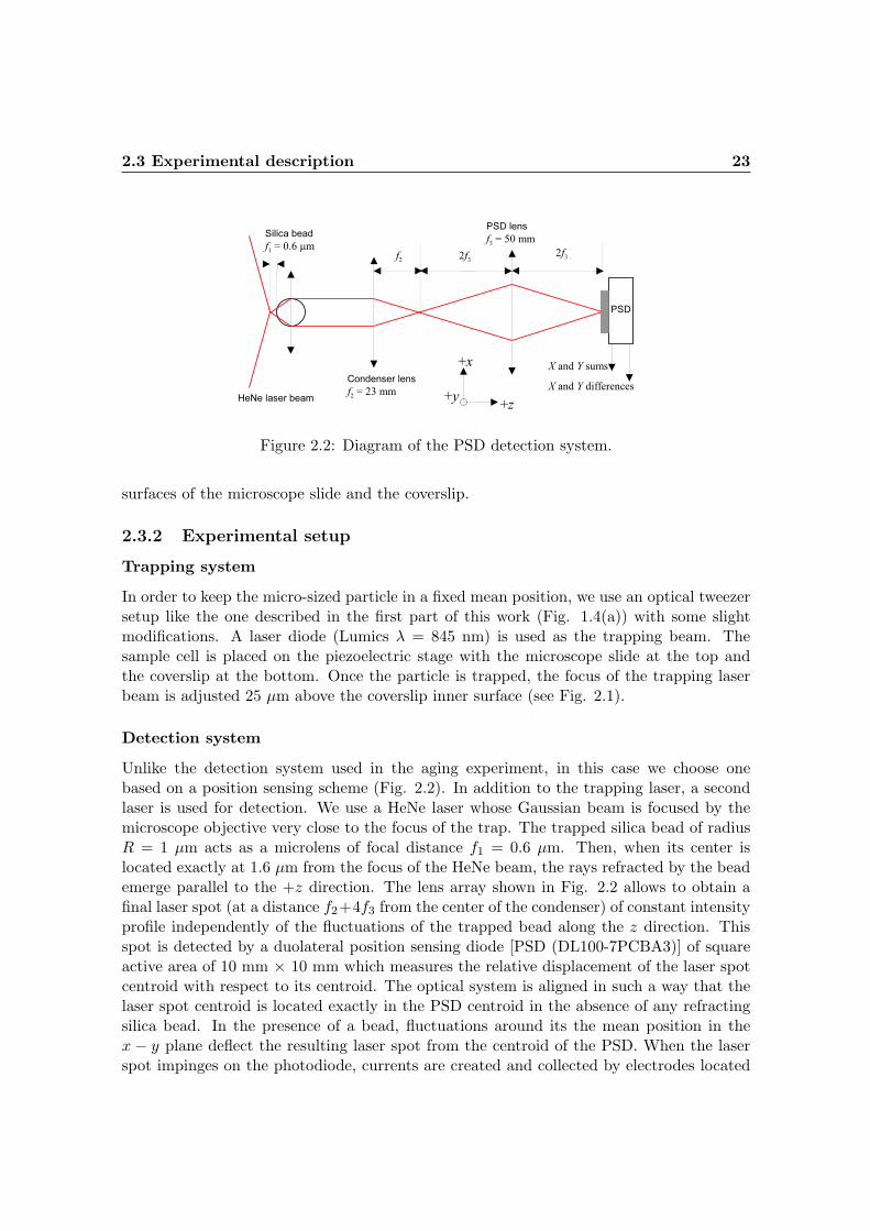
Figure 2.2: Diagram of the PSD detection system.

surfaces of the microscope slide and the coverslip.

2.3.2 Experimental setup

Trapping system

In order to keep the micro-sized particle in a fixed mean position, we use an optical tweezersetup like the one described in the first part of this work (Fig. 1.4(a)) with some slightmodifications. A laser diode (Lumics λ = 845 nm) is used as the trapping beam. Thesample cell is placed on the piezoelectric stage with the microscope slide at the top andthe coverslip at the bottom. Once the particle is trapped, the focus of the trapping laserbeam is adjusted 25 µm above the coverslip inner surface (see Fig. 2.1).

Detection system

Unlike the detection system used in the aging experiment, in this case we choose onebased on a position sensing scheme (Fig. 2.2). In addition to the trapping laser, a secondlaser is used for detection. We use a HeNe laser whose Gaussian beam is focused by themicroscope objective very close to the focus of the trap. The trapped silica bead of radiusR = 1 µm acts as a microlens of focal distance f1 = 0.6 µm. Then, when its center islocated exactly at 1.6 µm from the focus of the HeNe beam, the rays refracted by the beademerge parallel to the +z direction. The lens array shown in Fig. 2.2 allows to obtain afinal laser spot (at a distance f2+4f3 from the center of the condenser) of constant intensityprofile independently of the fluctuations of the trapped bead along the z direction. Thisspot is detected by a duolateral position sensing diode [PSD (DL100-7PCBA3)] of squareactive area of 10 mm × 10 mm which measures the relative displacement of the laser spotcentroid with respect to its centroid. The optical system is aligned in such a way that thelaser spot centroid is located exactly in the PSD centroid in the absence of any refractingsilica bead. In the presence of a bead, fluctuations around its the mean position in thex − y plane deflect the resulting laser spot from the centroid of the PSD. When the laserspot impinges on the photodiode, currents are created and collected by electrodes located

2.4 Preliminary results 24

at opposite edges. The currents collected at each edge are converted into voltages (X1, X2

along x and Y1, Y2 along y) that are processed in order to provide the difference outputsX1−X2, Y1−Y2 and the sum outputs X1 +X2, Y1 +Y2. The differences are then externallynormalized by the sums in order to obtain the coordinates (X = (X1 − X2)/(X1 + X2),Y = (Y1 − Y2)/(Y1 + Y2)) of the laser spot centroid. For simplicity, we record the Xcoordinate only. The position x(t) of the trapped bead with respect to its mean position isproportional to the position X of the laser spot centroid and the proportionality constantcan be determined by calibration of the apparatus. The signal X is filtered by a low-passfilter (Stanford SR640) with a cutoff of 4 kHz in order to get rid of high frequency modes,which are useless in this experiment. Once filtered, a time series {x(t)} of 1000000 datapoints are recorded at a scan rate of 8192 Hz for a given value of ∆T . Several spectra arerecorded in order to have good statistics when averaging to obtain 〈|x(ω)|2〉.

Temperature control system

A temperaute control system is needed in order to apply a temperature gradient of magni-tude ∆T/d in the +z direction across the ultrapure water layer, below the onset of RayleighBenard convection. An objective heating ring is placed around the metal jacket of the oil-immersion microscope objective (×63) in order to keep it at a constant high temperatureT1. The highest allowed temperature without damaging the objective is T1 = 37◦ C. Then,the metal jacket plays the role of a high temperature reservoir, keeping the temperature ofthe lower plate of the sample cell (the coverslip) at a constant value. On the other hand,a low temperature reservoir is implemented by means of a small chamber with circulatingwater placed above the upper plate (microscope slide) of the sample cell (see Fig. 2.1). Thecooling chamber consists on a metallic ring-shaped canal for water circulation encompassedbetween two heat-conducting sapphire windows. Water enters the chamber and flows (in alaminar regime) along the canal absorbing the heat transferred from the sample cell by thelower sapphire plate. Heat is evacuated when the water flow leaves the chamber, keepingthe microscope slide at a constant temperature T2. The lowest temperature that we canbe reached by the circulating water is T2 = 15◦ C without the effect of water condensationfrom air vapor on the optical surfaces. The inner surface of the canal is conic-shaped inorder to allow the whole deflected laser beams (both trapping and detecting beams) to passthrough the upper sapphire window, as shown in Fig. 2.1. The space between the innersurface of the canal and both saphire windows is filled with immersion oil to avoid a largemismatch of the optical path of the laser beams when passing through different opticalmedia in the chamber.

The critical value of the temperature difference that must be applied between bothreservoirs is calculated by means of Eq. (2.1). For the values of the parameters of thesystem used in the experiment, we obtain ∆Tc = 11 K. Then, we must choose ∆T < 11 Kin order to take the ultrapure water layer below the onset of convection.

2.4 Preliminary results 25

10−1

100

101

102

103

104

10−7

10−6

10−5

10−4

10−3

f (Hz)

<|x

(f)|

2 > (

V2 /

Hz)

experimentalLorentzian fit

(a)

10−1

100

101

102

103

104

10−7

10−6

10−5

10−4

10−3

f (Hz)

<|x

(f)|

2 > (

V2 /

Hz)

experimentalLorentzian fit

(b)

Figure 2.3: 2.3(a) Power spectral density of displacement fluctuations of the trapped par-ticle in the fluid at equilibrium (25◦ C with no heating and no cooling); 2.3(b) powerspectral density in the fluid at equilibrium (29◦ C with heating and cooling). In both casesthe plotted curves are averages over 10 spectra.

2.4 Preliminary results

No reliable results are obtained for the effect of non-equilibrium velocity fluctuations in thespectra of the trapped Brownian particle, given several technical difficulties encounteredduring the experiment, as discussed in the following.

First of all, we measure the power spectral density of displacements when the wholesystem is in equilibrium (∆T = 0) at room temperature (25◦ C). The power spectral densityis Lorentzian (Fig. 2.3(a)), as expected at equilibrium. In order to test the performance ofthe temperature control system inside the water layer, we increase both the temperatureof the objective heating ring and the circulating water in the upper chamber at T = 35◦

C. In this case, the system is also at equilibrium (∆T = 0) and the spectrum must beLorentzian, but we should expect an increase of the value of the corner frequency fc ∝ 1/ηand the low frequency level of the spectrum ∝ T/η since the value of the viscosity of waterη decreases. The expected relative magnitudes of such quantities at T = 35◦ C with respectto those at T = 25◦ C should be 1.24 for the corner frequency and 1.28 for the spectrumlevel. Figure 2.3(b) shows the power spectral density at T = 35◦, which is Lorentzian.However, the values of the relative magnitudes obtained from the Lorentzian fit are 1.07and 1.10, respectively. By looking for the temperature which corresponds to such ratios,we find the actual temperature of the water layer is 29◦ instead of 35◦ C. Then, we observethat there are large heat losses from the heating ring to the coverslip of the sample celland from the circulating water source to the the microscope slide and there is not enoughtemperature control even at equilibrium. Thus, under this experimental conditions it isvery difficult to take the system close enough and below the critical temperature difference∆Tc = 11 K where the amplitude of non-equilibrium velocity fluctuations is extremelyenhanced. However, we could not improve the temperature control system due to lack oftime.

2.4 Preliminary results 26

10−1

100

101

102

103

104

10−7

10−6

10−5

10−4

10−3

10−2

f (Hz)

<|x

(f)|

2 > (

V2 /

Hz)

(a)

10−1

100

101

102

103

104

10−7

10−6

10−5

10−4

10−3

f (Hz)

<|x

(f)|

2 > (

V2 /

Hz)

experimentalLorentzian fit

(b)

Figure 2.4: 2.4(a) Power spectral density of displacement fluctuations of the trapped parti-cle in the presence of a temperature gradient with interacting small particles; 2.4(a) powerspectral density in the presence of a temperature gradient. The plotted curve is the av-erage over five spectra with neither any apparent interaction with small particles nor anyapparent horizontal convection.

Another major problem encountered during the application of the vertical temperaturegradient is the presence of a uniform horizontal water flow around the trapped particle evenbelow the theoretical critical temperature difference ∆Tc = 11 K. This flow is thought tobe due to non-zero horizontal temperature gradients in the microscope slide, leading to auniform horizontal convective motion of the fluid close to the microscope slide. The forceof this convective flow is strong enough to drag free Brownian particles close to the trappedone and then strongly perturbing its motion. Even in the absence of free beads close tothe trapped one, very small particles that cannot be filtered by the 0.22 µm microporefilter get close to the trapped bead and interact with it, modifying enormously the lowfrequency side (f < 2 Hz) of the spectrum, as shown in Fig. 2.4(a). Unfortunatly, this isthe frequency range where non-equilibrium hydrodynamic fluctuations are expected to takeplace and their effect on the motion of the trapped bead is easily hidden by any influence ofneighboring small particles. By keeping only the time series with no apparent interactionsof small particles and no apparent horizontal convective flow, we obtain the power spectraldensity curve shown in Fig. 2.4(b). Unlike spectra at equilibrium (Figs. 2.3(a) and 2.3(b)),in this case it is possible to observe a slight increase of the spectrum level for f < 1 Hz, whichsuggests the effect of slow non-equilibrium hydrodynamic fluctuations due to the verticaltemperature gradient across the fluid layer, as expected from the calculations carried out inSection 2.2. However, given the lack of knowledge of the actual temperature gradient andthe possible existence of additional perturbing sources, this increase could be an artifactand not the actual effect of non-equilibrium velocity fluctuations of water.

2.5 Conclusion and perspectives 27

2.5 Conclusion and perspectives

We have roughly estimated the possible effects of non-equilibrium hydrodynamic fluctu-ations on the motion a micro-sized particle immersed in water and trapped by opticaltweezers. Unlike scattering experiments performed in the past, in this case we are inter-ested in a local effect. We find that only velocity fluctuations could be non-negligible andmodify the lower frequency side of the power spectral density of displacement fluctuations.

We must be aware that the results obtained here are very preliminary and they are notcompletely reliable given the several sources of low frequency noise observed during themeasurements. Then, in order to enhance the effect, we must look for an optimal value ofthe Rayleigh number corresponding to a good compromise between the critical slowing downand the amplitude of fluctuations below the onset of instability. An analytical calculationof the expression for the power spectral density of velocity fluctuations in the x− y planeis also needed in order to know the actual contribution of non-equilibrium fluctuations tothe power spectral density of the probe particle. We need to improve in the future thetemperature control system in order to take the system close enough to and below theonset of convection and be able to resolve the contribution of non-equilibrium fluctuations.One should also take into account the presence of possible additional hydrodynamic effectssince the probe particle was trapped at 25 µm above the inner surface of the lower platewhere viscosity could damp the non-equilibrium effect. One possible direction is the use ofvideo microscopy in order to study the motion of multiple free micro-sized particles in avery thin Rayleigh-Benard cell.

Bibliography

[1] G. Parisi, Phys. Rev. Lett. 79, 3660 (1997).

[2] W. Kob and J.L. Barrat, Europhys. Lett. 46, 5 (1999).

[3] L.F. Cugliandolo, J. Kurchan, and L. Peliti, Phys. Rev. E 55, 3898 (1997).

[4] S.M. Fielding and P. Sollich, Phys. Rev. E 67, 011101 (2003).

[5] D. Herisson and M. Ocio, Phys. Rev. Lett. 88, 257202 (2002).

[6] J. Kurchan, Nature 433 (2005).

[7] B Abou, D. Bonn, and J. Meunier Phys. Rev. E 64, 021510 (2001).

[8] S. Jabbari-Farouji1, E. Eiser, G. H. Wegdam, and D. Bonn, J. Phys.: Condens. Matter16, (2004)

[9] N. Ghofraniha, C. Conti, and G. Ruocco, Phys. Rev.B 75, 224203 (2007).

[10] L. Bellon, S. Ciliberto, and C. Laroche, Europhys. Lett. 53, 511 (2001); L. Bellon andS. Ciliberto, Physica D 168-169, 325 (2002); L. Buisson, L. Bellon, and S. Ciliberto,J. Phys. Cond. Matt. 15, S1163 (2003).

[11] B. Abou and F. Gallet, Phys. Rev. Lett. 93, 160306 (2003).

[12] S. Jabbari-Farouji, D. Mizuno, M. Atakhorrami, F.C. MacKintosh, C.F. Shmidt, E.Eiser, G.H. Wegdam, and D. Bonn, Phys. Rev. Lett. 98, 108302 (2007).

[13] N. Greinert, T. Wood, and P. Bartlett, Phys. Rev. Lett. 97, 265702 (2006).

[14] S. Jabbari-Farouji, D. Mizuno, G.H. Wegdam, F.C. MacKintosh, C.F., and D. Bonn,arXiv:0804.3387v1.

[15] A. Ashkin, Phys. Rev. Lett. 24, 4 (1970).

[16] J. Bechhoefer and S. Wilson, Am. J. Phys. 70, 4 (2002)

[17] M. Capitanio, G. Romano, R. Ballerini, M. Giuntini, and F.S. Pavone, Rev. Sci.Instrum. 73, 4 (2002).

BIBLIOGRAPHY 29

[18] L. Berthier and J.-L. Barrat, Phys. Rev. Lett. 89, 095702 (2002).

[19] H.Z. Cummins, Journal of Non-Crystalline Solids 353, (2007)

[20] D. Bonn, S. Tanase, B. Abou, H. Tanaka, and J. Meunier, Phys. Rev. Lett. 89, 015701(2002).

[21] D. Bonn, H. Kellay, H. Tanaka, G. Wegdam, and J. Meunier, Langmuir 15 (1999).

[22] P. Jop, A. Petrosyan, and C. Ciliberto, Phys. Rev. Lett (submitted, LEK 1023) (2007).

[23] B.M. Law, R.W. Gammon, and J.V. Sengers, Phys. Rev. Lett. 60, 15 (1988).

[24] P.N. Segre, R.W. Gammon, J.V. Sengers, and B.M. Law, Phys. Rev. A 45, 2 (1992).

[25] A. Vailati and M. Giglio, Phys. Rev. Lett. 77, 8 (1996).

[26] J.M. Ortiz de Zarate and J.V. Sengers, Physica A 300, (2001).

[27] J.M. Ortiz de Zarate and J.V. Sengers, Phys. Rev. E 66, 036305 (2002).

[28] J.M. Ortiz de Zarate and J.V. Sengers, JSTAT 115, 516 (2002).

[29] J. Oh, J.M. Ortiz de Zarate, J.V. Sengers, and G. Ahlers, Phys. Rev. E 69, 021106(2004).