Experimental Study of Mobile Air Conditioning System Transient Behavior

ACRCTR-102

For additional information:

Air Conditioning and Refrigeration Center University of Illinois Mechanical & Industrial Engineering Dept. 1206 West Green Street Urbana, IL 61801

(217) 333-3115

C. D. Collins and N. R. Miller

July 1996

Prepared as part of ACRC Project 51 Design and Control of Mobile Air-conditioning Systems

N. R. Miller and W. E. Dunn, Principal1nvestigators

The Air Conditioning and Refrigeration Center was founded in 1988 with a grant from the estate of Richard W. Kritzer, the founder of Peerless of America Inc. A State of Illinois Technology Challenge Grant helped build the laboratory facilities. The ACRC receives continuing suppon from the Richard W. Kritzer Endowment and the National Science Foundation. The following organizations have also become sponsors of the Center.

Amana Refrigeration, Inc. Brazeway, Inc. Carrier Corporation Caterpillar, Inc. Dayton Thennal Products Delphi Harrison Thennal Systems Eaton Corporation Electric Power Research Institute Ford Motor Company Frigidaire Company General Electric Company Lennox International, Inc. Modine Manufacturing Co. Peerless of America, Inc. Redwood Microsystems, Inc. U. S. Anny CERL U. S. Environmental Protection Agency Whirlpool Corporation

For additional information:

Air Conditioning & Refrigeration Center Mechanical & Industrial Engineering Dept. University of Illinois 1206 West Green Street Urbana IL 61801

2173333115

Abstract

An experimental study of the the transient behavior of an automobile arr

conditioning system was performed. The experiments were conducted on an original

equipment air conditioning system modified for laboratory investigation. Qualitative results

showing a clear relationship between refrigerant charge and mean clutch cycling period,

and between refrigerant charge and the transient behavior of the evaporator outlet

refrigerant temperature, were obtained.

A five-factor, two-level, designed experiment was performed to determine the

sensitivity of the clutch cycling period of the air conditioning refrigeration system to small

(8%-15%) changes in: condenser air flow rate, condenser air inlet temperature, evaporator

air inlet temperature, compressor speed, and refrigerant mass. The values chosen for each

factor were based on a nominal operating condition which assumed a vehicle speed of 60

mph, and an air conditioning system operating on maximum cold setting, full recirculation,

and maximum evaporator speed. The test facility permitted the control of condenser and

evaporator air flow rates and inlet air temperatures, compressor speed, and refrigerant

charge. Evaporator fan speed was set at the same value for all tests, and all tests were run

dry coil.

For the range of variables studied, experimental results showed that refrigerant

charge loss corresponded to a shortening of the mean clutch cycling period and a decrease

in the variance of the mean clutch cycling period. Experimental results further showed that

the transient behavior of the evaporator refrigerant outlet temperature, following each clutch

engagement, was clearly a function of refrigerant charge. A parameter, Time to

Temperature Turning, was defined which adequately describes this behavior in terms of

time and temperature only.

The results imply that a strong possiblity exists for the development of a real-time,

on-line refrigerant charge loss diagnostic device based on temperature measurements and

time.

Table of Contents Page

List of Tables .................................................................... vi

List of Figures .................................................................. vii

1. I~1rIt()J)1JCTI()~ •.••..••••••.•.••••••.••••••••••..••••.•..• ••...•.•.•.••..•.. 1 1.1 Motivation .................................................................. 1 1.2 Scope of Work .............................................................. 1

1.2.1 Refrigerant Charge Loss Detection ••••••..••••••.•••..•...•.•.....• 1 1.2.2 Experimental Facility Modifications and Analysis •••••..•.•••.... 2

2. LIT~It~T1JIt~ 1t~"I~~ •••••.•...•.••.•.••••••••••••••....•.•.......•.• .... 3 2.1 Fault Diagnosis ............................................................. 3

2.1.1 Fault Detection ....................................................... 3 2.1.2 Fault Diagnosis ...................................................... 4

2.2 Statistics .................................................................... 4 2.3 Air Conditioning and Refrigeration' Systems .•••.•••••••.•.••.•••......•. 5 2.4 Experimental Facility ...................................................... 5

3. ~XP~ItIM~NTAL F~CILITY J)~SClUPTI()~ ••••.•••••••••••..••••.. 7 3.1 ()vervielV .................................................................... 7

3.1.1 Motor Controller Terminology ..•••.•...•••••.•.•.••••••.••..•.....• 7 3.2 Condenser Air FlolV System ............................................... 9

3.2.1 Instrumentation ...................................................... 9 3.2.2 Mechanical .......................................................... 12 3.2.3 Electrical ............................................................ 13

3.3 Evaporator Air Flow System ............................................. 13 3.3.1 Instrumentation ..................................................... 13 3.3.2 3.3.3

Mechanical .......................................................... 14 Electrical ............................................................ 14

3.4 Refrigeration System ...................................................... 15 3.4.1 Instrumentation ..................................................... 15 3.4.2 3.4.3

3.5 Data 3.5.1 3.5.2

Mechanical .......................................................... 1 8 Electrical ............................................................ 20 Acquisition System .................................................. 2 0 Components ......................................................... 21 Software ............................................................. 23

3.6 Environment Control System ............................................. 2 3 3.6.1 Components ..................... ~ ................................. .. 24

4. It~FItIG~AA~T CH~ItG~ L()SS ~XP~ItIM~~TS •••.•••....••.•.. 2 7 4.1 Principles .................................................................. 2 7

4.1.1 Charge Loss Indications ........................................... 31 4.1.2 Practical Measurements ............................................ 31

4.2 Charge Optimization ...................................................... 3 2 4.2.1 Definition of Optimum Charge ........••••...•••.•.•.•••...•.•••.•• 3 2 4.2.2 Test Conditions ..................................................... 3 3 4.2.3 Test Method ......................................................... 33 4.2.4 Results ............................................................... 3 4

4.3 Experiment Design ........................................................ 3 6 4.3.1 Terminology ......................................................... 3 7 4.3.2 Fractional Factorial Design ••••.•.•••••.•.•..••••••••..•••..••.•••• 3 8

iv

4.3.3 Selection of Factors and Levels ••••••.•••.•.•....•..•.•.•.....•..• 4 0 4.4 Test Procedure ............................................................ 4 0 4.5 Clutch Cycling: Main Effects And Interactions •••..•...•.•......•.•... 41 4.6 Clutch Cycling: Analysis of On-Cycle and Off-Cycle Behavior ...•.• 4 6

4.6.1 Duty Cycle Analysis ................................................ 4 6 4.6.2 Evaporator Pulldown Analysis 1 •••••••••••.••.••••••...••...•..•. 48 4.6.3 Evaporator Pulldown Analysis 2 •.•••.••.•.••.•••••.•.•.•.•.•..... 49

5. CONCLUSIONS ............................................................. 5 2 5.1 Summary of Work and Scope of Results ••••••••••••••.•.•......•••.••• 5 2 5 . 2 Conclusions ............................................................... 5 2 5.3 Recommendations and Future Work ••••••••.•••••••••••••••.••.•...••.• 5 3

List of Refer-ences .............................................................. 5 5

Appendix A. Pressure Transducer Calibration .•.••.•.................• 5 8

Appendix B. Zone Box Diagrams ........................•.....•.......... 6 2

Appendix C. Programmable Logic Controller System .•............• 6 9

Appendix D. Charge Optimization Test Plans •.•................•...•.• 8 5

Appendix E. Experimental Facility Energy Balance Validation ..• 88

Appendix F. Clutch Cycling Data •••••••.••••••.•.•.•••......•...•..•••••. 9 4

v

List of Tables

Page

Table 4.1 Test Conditions for Charge Optimization Experiment 1 .............................. 33

Table 4.2 Key for Coded Experiment Design Notation .......................................... 37

Table 4.3 Coded Experiment Design .............................................................. 39

Table 4.4 5-Factor, 2-Level Fractional Factorial Experiment Design ........................... 40

Table 4.5 Key for Coded Experiment Design Notation .......................................... 41

Table 4.6 Clutch cycling period results from a 16-run half-fraction design with 5 variables .................................................................................... 42

Table 4.7 Results from repeated 16-run half fraction design with 5 variables ................. 43

Table 4.8 Experiment 1: Main Effects and Interactions .......................................... 44

Table 4.9 Experiment 2: Main Effects and Interactions .......................................... 44

Table 4.10 Experiment 2: Analysis of Main Effects and Interactions ............................ 45

Table 4.11 Analysis of Off-Cycle Time for all runs ................................................ 47

Table 4.12 Analysis of On-Cycle Pulldown Transient at the Evaporator Outlet. .............. 49

Table A.l Compressor Discharge Pressure Transducer Calibration Check .................... 61

Table A.2 Condenser Inlet Pressure Transducer Calibration Check ............................ 61

Table B.l Data Acquisition System Channel Cross Reference ....... , .......................... 68

Table D.l Single Point Charge Optimization Test Plan ........................................... 86

Table D.2 Varying Parameters Charge Optimization Test Plan .................................. 87

Table E.l Condenser and Evaporator Energy Balance Error Statistics ......................... 89

Table E.2 Comparison of Air Volume Flow Rate Measurement: Venturi vs. Hot Wire Anemometer ............................................................................... 90

Table F.l Clutch Cycling Data .................. , ................................................... 94

vi

List of Figures

Page

Figure 3.1 Test Facility Schematic ..................................................................... 8

Figure 3.2 Parallel Thermocouple Circuit. .......................................................... 11

Figure 4.1 R134a Pressure Enthalpy Diagram with Refrigeration Cycle ........................ 28

Figure 4.2 Evaporator temperature as a function of refrigerant charge and compressor speed ....................................................................................... 35

Figure 4.3 Evaporator temperatures as a function of refrigerant charge ......................... 36

Figure 4.4 Run 2-5: Time history of evaporator outlet refrigerant temperature and pressure .................................................................................... 47

Figure 4.5 Runs 2-4 and 2-12: Time history of evaporator outlet refrigerant temperature and pressure ............................................................................... 48

Figure 4.6 Runs 3-15 and 3-16: Time history of evaporator outlet refrigerant temperature and pressure ............................................................................... 50

Figure 5.1 A scheme for measuring the mass of refrigerant in a heat exchanger ............... 54

Figure A.1 Liquid Line Venturi Inlet Gage Pressure Transducer Calibration ................... 59

Figure A.2 Compressor Suction Gage Pressure Transducer Calibration ........................ 60

Figure B.1 Zone Box Diagram Drawing Notes ..................................................... 63

Figure B.2 Condenser Loop Zone Box Diagram .......... , ........................................ 64

Figure B.3 Refrigerant System Zone Box Diagram ................................................ 65

Figure B.4 Evaporator Loop Zone Box Diagram (1 of 2) ......................................... 66

Figure B.5 Evaporator Loop Zone Box Diagram (2 of 2) ......................................... 67

Figure E.1 Steady-State Energy Balances: Evaporator and Condenser .......................... 88

Figure E.2 Charge optimization: Heat transfer rates versus refrigerant charge level. .......... 91

Figure E.3 Energy balance errors as a function of refrigerant charge ............................ 91

Figure E.4 Air side heat transfer rate as a function of refrigerant charge ........................ 93

Figure F.1 Experiment 2: Evaporator outlet refrigerant temperature and pressure time histories [Runs 2-1 through 2-4 ; Runs 2-9 through 2-12] .......................... 95

Figure F.2 Experiment 2: Evaporator outlet refrigerant temperature and pressure time histories [Runs 2-5 through 2-8; Runs 2-13, 2-14, 3-15, 3-16] .................... 96

Vll

1. IN1RODUCTION

1. 1 Motivation Refrigerant leakage from mobile air conditioning refrigeration systems contributes to

environmental pollution and eventually leads to reduced cooling performance. Compressor

lubrication in mobile air conditioning refrigeration systems is provided by oil that circulates

with the refrigerant. Therefore, inadequate refrigerant circulation due to low refrigerant charge

may cause reduced compressor lubrication. Reduced compressor lubrication can lead to

premature mechanical failure of the compressor. Under certain operating conditions, in

systems employing a suction pressure controlled compressor clutch, refrigerant charge loss

may induce frequent clutch cycling. Excessive clutch cycling may cause premature clutch

failure and may adversely affect driveability, fuel economy and engine idling control.

The goal of early fault detection and diagnosis is to permit time for automatic or manual

corrective actions to be taken before catastrophic system failures occur[lJ. An early warning in

a mobile air conditioning system equipped with a fault diagnosis and operator warning system

would trigger maintenance actions like a refrigeration system inspection and repair. Further

uncontrolled leakage would be prevented, and air conditioning system failure in operation

would be avoided.

1.2 Scope of Work This thesis documents work undertaken as part of the University of lllinois' Air

Conditioning and Refrigeration Center Project 51, Diagnostics and Control of Mobile Air

Conditioning Systems. Two of the project goals are addressed in this report: (1) development

of a refrigerant charge loss diagnostic tool using measures of the transient behavior of the

system, and (2) experimental characterization of transient and steady-state performance of

mobile air conditioning systems.

1. 2.1 Refrigerant Charge Loss Detection

Fault detection is concerned with detecting changes in the operating states of a system

compared to the "normal," or design, operating states. This defInition implies that we have

prior knowledge of the normal operating state, and also of the sensitivity of the refrigeration

system performance to changes in relevant system parameters such as air side temperatures and

flow rates, compressor speed and refrigerant charge.

We defIned normal operating conditions for our test rig based on information obtained

from our industrial sponsors. We supplemented this information with data from laboratory

testing. We performed a set of laboratory tests, over a range of operating conditions, which

documented the performance of our air-conditioning system in steady-state and transient

(cycling clutch) operation. We used the data obtained from these experiments in our charge

1

loss study.

We made two major studies of the data obtained in our experiments. First, we

computed the main effects and second-order interaction effects of the controlled variables

mentioned above on the clutch cycling period. Second, we studied the refrigerant temperature

and pressure measured at the evaporator outlet, the compressor discharge and in the liquid line

upstream of the expansion device. The second study focused on identifying transient behavior

that could be uniquely associated with charge loss.

1.2.2 Experimental Facility Modifications and Analysis The design and construction of the test facility is thoroughly documented in [2, 3].

Part of the work reported here concerns modifications we made to the experimental facility.

These modifications included (a) the installation and validation of a new data acquisition

system, and (b) the installation of a programmable logic controller to implement the

environmental controller function of the test facility.

We made a considerable effort to clarify and quantify the uncertainty in data obtained

from the test facility. We explicitly computed experimental uncertainties in direct

measurements and in calculations made from these measurements, with specific attention paid

to heat transfer calculations. This effort included:

(a) recalibration of refrigerant side gage pressure and heat exchanger differential pressure transducers, and

(b) comparison of air flow rates measured with the installed venturi flow tubes and associated transducers to air flow rates obtained by duct traverses with a hot wire anemometer.

We readdressed the problems associated with obtaining satisfactory agreement between

the air side and refrigerant side heat transfer measurements, documented in [2]. We concluded

that the explanations and solutions provided in [2] were partially inadequate, particularly with

respect to condenser air side temperature measurement. We provide guidance for further

improvements during the next overhaul of the test facility.

We note here that the systematic error in condenser air side heat transfer measurement is

only marginally relevant to the refrigerant charge loss study. The refrigerant charge loss study

considered only refrigerant side measurements. However, accurate measurement of condenser

air side heat transfer is critical to another goal of this project, validation of a transient computer

model of the mobile air-conditioning system. Without an accurate measurement of condenser

air side heat transfer, experimental estimation of the state of the refrigerant exiting the

condenser when the refrigerant is in a 2-phase state will be uncertain and inconclusive.

2

2. LITERATURE REVIEW We drew on literature from several areas of research:

(a) fault diagnosis, including survey papers, tutorials, and reports of specific mechanical engineering related applications,

(b) statistics, particularly statistical design and analysis of experiments,

(c) air conditioning and vapor compression refrigeration systems, and

(d) experimental facility design, construction and instrumentation.

2. 1 Fault Diagnosis Fault diagnosis is typically associated with the broader field of control systems.

General principles and the state of the art are reviewed with clarity in occasional survey

papers and tutorials appearing in IEEE and IFAC publications. We acquired the standard

fault diagnosis tenninology and concepts through our review of several such survey papers

and tutorials [1, 4-10]. Specific theoretical and practical applications of fault diagnosis

have been reported for refrigeration systems, internal combustion engines, and machine

tools. We referred to a number of articles documenting mechanical engineering and

process engineering applications of fault diagnosis concepts [11-16].

The goal of this thesis project entailed experimental identification of transient

behaviors of a mobile air conditioning refrigeration system, which could be used as

symptoms in an automated fault detection and diagnosis system. Symptom is a term from

the fault diagnosis literature. In the following discussion, the tenninology, major concepts,

and current trends in fault detection and diagnosis are briefly presented.

2.1.1 Fault Detection

Fault detection is accomplished by analytic and heuristic symptom generation [1,

9]. Symptoms are defmed in [9] as facts on which a fault diagnosis is based. In [1]

analytic symptoms are further defined as

"the results of the limit value checking of measurable signals, signal or process model fault detection methods and change detection."

Signal or process fault detection methods refer to the generation and analysis of

residuals based on: (a) state-space techniques like parameter estimation and state estimation,

or (b) parity equation (polynomial) techniques. Residuals measure the deviation of the

actual process from the nominal non-faulty process. A mathematical model, driven by

measurable inputs, is required to estimate or predict the non-faulty outputs, states or

parameters of the process. Such a model is also required to calculate unobservable states or

parameters of the actual process. Hence, the term model-based fault detection is applied to

analytic symptom generation. In other words, analytic symptoms are numerical and

quantifiable. Analytic fault detection occurs when residuals are generated which depart by

3

an unacceptable amount from their nonnal values. The defInition of 'unacceptable' is an

engineering design problem, and depends strongly on the requirements of the process

being considered.

Heuristic symptoms are based on qualitative infonnation associated with

observations and judgments made by a human operator [1, 9]. Such symptoms are

included in a fault diagnosis reasoning process through some fonn of interactive interface

with an operator. Heuristic symptoms are characterized by a verbal description or "vague"

number.

A third class of symptoms, called process history and fault statistics, are described

in [9]. These symptoms, as the name suggests, are obtained through numerical analysis or

qualitative assessment of the general status of the process. Process history and fault

statistics are further classifIed as heuristic, or, if they are clearly quantitative and

comparable to some type of nominal model, analytic.

2.1. 2 Fault Diagnosis

Automatic fault diagnosis is the identifIcation of a fault, based on deductions made

from a set of observed symptoms. A number of methods have been applied to fault

diagnosis problems, including: knowledge-based reasoning [6-9], fault tree analysis [10],

expert systems [13], neural networks [17] and statistical pattern recognition [16, 18].

Sorsa [17] argues that neural networks present the most promising method for

diagnosing faults in complex systems for which precise models are difficult or impossible

to obtain. [17] succinctly describes the chief technical obstacle in rival methods,

specifIcally:

(a)

(b)

the difficulty in obtaining accurate process models for use in state or parameter estimation techniques, and

the difficulty in developing a sufficiently extensive and accurate database of rules for use in a rule-based expert system.

In [17], pattern recognition techniques are claimed to provide the best solution

when the process model is unknown or complex, and neural networks are cited as a viable

method for pattern recognition. In [16], Rossi claims to successfully detect and diagnose

refrigerant leaks in a vapor compression refrigeration system. Rossi's method employs a

combination of model-based symptom generation with fault detection and diagnosis based

on statistical pattern recognition, and requires the system to be operating in steady-state.

2.2 Statistics

It is known that the mass of refrigerant charge in a vapor compression refrigeration

system strongly influences system perfonnance. Refrigeration system perfonnance is also

affected by compressor speed, and by the flow rates, temperatures and relative humidities

4

of the condenser and evaporator air streams. One of the parameters that is affected by

varying the refrigerant charge in a pressure cycled clutch type of mobile air conditioning

system is the time period over which the compressor clutch cycles. This measure is

currently used in a limited way to manually diagnose refrigerant charge loss during vehicle

maintenance [19].

In the laboratory, we controlled the heat exchanger air flow rates, the heat

exchanger air inlet temperatures, the compressor speed, the clutch cycling pressure

setpoints and the refrigerant charge. We employed a fractional factorial experiment design

to determine the effects of a subset of these variables on clutch cycling period, specifically:

(a) condenser air flow rate and inlet temperature,

(b) evaporator air inlet temperature,

(c) compressor speed, and

(d) refrigerant charge.

We referred extensively to Box and Hunter [20] for guidance on implementing and

analyzing a designed experiment. We referred to two other basic statistics texts [21, 22]

for descriptions and examples of a number of concepts, including standard deviation,

standard error and t-tests.

2.3 Air Conditioning and Refrigeration Systems

Air conditioning and refrigeration system fundamentals are well known. Of the

many similar basic references available, we relied on [23, 24]. An experimental and

analytical study characterizing the effects of varying refrigerant charge on the performance

of a residential air conditioner is reported in [25]. The effects of varying refrigerant charge

in a mobile air conditioning refrigeration cycle are reported in [26]. A refrigerant

monitoring system based on mechanical sensing of the quality of the refrigerant flowing

from the condenser is described in [14]. Rossi [16] developed a refrigerant leak detection

method for residential air-conditioners based on model-based and statistical pattern

recognition techniques. Fasolo and Seborg [12] performed a feasibility study of a fault

detection method based on calculating and analyzing changes in a performance index

calculated for a closed loop HV AC controller.

2.4 Experimental Facility

The technical reports produced by the Air Conditioning and Refrigeration Center at

the University of lllinois provide many theoretical and practical discussions of test stand

design and construction for air conditioning and refrigeration studies. The development of

our test facility is documented, in reverse chronological order, in Weston [3], Rubio-Quero

[2] and Micheal [27]. Heun [28] discusses problems associated with air side temperature

5

measurement! in the presence of severe spatial temperature gradients, and provides an

effective solution that we adapted to our test facility.

We revisited the topic of experimental uncertainty addressed by Weston [3] with the

goal of more explicitly evaluating the uncertainties in the quantities we calculate from our

basic measurements of temperature, pressure and differential pressure. These quantities

include refrigerant properties, mass flow rates and heat transfer rates. Doebelin [29]

contains a straightforward discussion of error propagation in experimental calculations2•

Heun [28] devotes considerable attention to quantifying the experimental uncertainty in his

study, and Staley [30] includes a detailed uncertainty analysis in his report on steady-state

refrigerator performance.

1 Ref. [28] pp. 93-95.

2 Ref. [29] pp.58-67.

6

3. EXPERIMENTAL FACILITY DESCRIPTION The experimental facility used in this study is located in room 115K Mechanical

Engineering Laboratory at the University of lllinois. The following discussion briefly

describes: (a) major subsystems, and (b) the subsystem components, functions, principles of

operation and interconnections. [2] and [3] discuss the design and construction of the test

facility, and the measurement principles and practices employed in design and installation of the

instrumentation system. The changes we made to each subsystem are documented in detail in

the following discussion.

3.1 Overview

The test facility is designed to permit the collection of high-quality quantitative and

qUalitative data from a mobile air-conditioning system operating over a wide range of steady­

state and transient operating conditions. The following physically distinct major subsystems

comprise the test facility:

(a) the condenser air flow system,

(b) the evaporator air flow system,

(c) the refrigeration system,

(d) the data acquisition system, and

(e) the environmental control system.

Figure 3.1 is a schematic diagram of the test facility which illustrates the major

subsystems, components and system interconnections. We will refer to Figure 3.1 in the

following descriptions of the test facility subsystems.

3.1.1 Motor Controller Terminology

Our test facility uses squirrel cage, AC induction, electric motors to drive the condenser

blower, the evaporator blower, and the compressor belt drive. A device that distributes

electrical power to a motor, permits the motor to be started and stopped, and provides overload

protection is usually referred to as a motor starter or motor controller. A device that converts

standard electric power to variable frequency electric power for distribution to a motor for

variable speed operation is called a variable speed drive. A variable speed drive that generates

variable frequency electric power using pulse width modulation is referred to as an inverter

[3]. The terms motor controller, variable speed drive, and inverter, are interchangeable to

some extent. The devices installed in our test facility for motor control integrate the functions

of the motor controller and the inverter we have described. We will refer to these devices in the

rest of the discussion as inverters, in accordance with the manufacturer's description.

7

8 CI.l

~

00 I u

Condenser Plenum

Flow

Screen.

t

Pres..ure Relief Valve

Refrigerant/Oil Mixture Sampling A .. o;cmbly

Oil Concentration (not installed) Sensor

Blower Speed Setpoint

Venturi Flow Tube

Recireu1ate to Plenum and/or Exhaust to Hood

01 Compressor Speed

Setpoint

Barometer

Drawn by: Weston (1195) Revised by: Collin. (6196)

Orifice Tube

• Tbermoeoup\e Reference Bath

Figure 3.1 Test Facility Schematic

Sight Tube

Evaporator Plenum

Venturi Flow Tube

Recireulate to Plenum

Flow

•

~ ~ o ~

~

3.2 Condenser Air Flow System

The test facility is required to simulate air flow conditions at the inlet of the air

conditioning system condenser. The condenser air flow system provides precise

measurement and control of air flow over the condenser. The condenser air flow system is

equipped with mechanical, electrical and instrumentation subsystems which allow the

researcher to: (a) control condenser air flow rate, (b) control condenser inlet air dry bulb

temperature, and (c) collect temperature, pressure,relative humidity and flow rate data.

See Figure 3.1 for a schematic diagram illustrating the system layout and interconnections.

For a detailed mechanical drawing of the condenser air flow system, refer to Figure 2.2 in

[3].

3.2.1 Instrumentation

Overview

In the following discussion, we present the basis for the instrumentation scheme

installed in the condenser air flow system. The condenser air flow system is instrumented

to permit the calculation of the heat rejected by the condenser to the air stream. The

condenser heat transfer rate may be expressed as

where

Q = heat transfer rate (BTU / hr)

m = mass flow rate (Ibm / hr)

hin = inlet air enthalpy (BTU / Ibm)

hour = outlet air enthalpy (BTU / Ibm).

(3.1)

The moist air enthalpy, h, and mass flow rate, m, are not measured directly. We calculate

these quantities from direct measurements of temperature, total pressure, relative humidity

and differential pressure.

Three independent, intensive thermodynamic variables are required to uniquely

specify moist air enthalpy, h. We directly measure the response of dry bulb temperature,

total pressure, and relative humidity instruments, and then evaluate the moist air enthalpy

using EES, a software package which includes thermodynamic property evaluation

functions. The moist air mass flow rate is calculated by evaluating the basic relation

governing incompressible flow in venturi devices. This relation is derived by applying the

laws of conservation of mass and energy (in the form of the Bernoulli equation for

horizontal flow) to a control volume from the inlet tap to the outlet tap of the venturi device.

A detailed discussion of venturi flow tube theory and operation is presented by Weston in

9

[3]3. The basis of our venturi instrumentation scheme is illustrated by considering the ideal

form of the incompressible flow venturi relation

where

m = mass flow rate (lbmlhr)

f32 = ~ I Al = area ratio

Al = inlet area (fe)

~ = throat area (ft2)

(3.2)

gc = English Engineering unit system force constant (ft -lbmllbf - S2)

PI = density (lbmlft3)

~ = inlet pressure (lbf/ft2)

~ = throat pressure (lbf/ft2).

The differential pressure generated by air flowing in the venturi flow tube, P1-P2' is

obtained by direct measurement of the response of a differential pressure transducer. The

moist air density is calculated in EES using moist air temperature, pressure and relative

humidity data obtained by direct measurement.

We have presented the basis for the instrumentation scheme in the condenser air

flow system. In the following discussion we present details pertaining to the temperature,

pressure, differential pressure and relative humidity measurements.

Temperature

We measure the moist air dry bulb temperature at: (a) the condenser inlet, (b) the

condenser outlet, (c) the relative humidity probe located in the blower inlet section, and (d)

the venturi inlet. The condenser inlet air temperature is measured with a 9-point

thermocouple array, wired in parallel. The condenser outlet air temperature is measured

with a 40-point, parallel-wired thermocouple array. The parallel wiring arrangement

generates a voltage which corresponds to the average of the. voltages generated by the

individual thermocouples. Figure 3.2 illustrates the conceptual basis of the parallel wiring

arrangement for thermocouple circuits. This wiring method permits the spatial average

temperature of the air flow to be measured, and requires only one reference thermocouple.

3 pp. 102-128.

10

Parallel and series (thennopile) multiple thennocouple array techniques are further

discussed in [3], [28], [31] and [29]. Figure 2.10 and 2.13 in [2] illustrate the

arrangement and numbering of the inlet and outlet grid thennocouple junctions. The

thennocouples installed in the test facility are identified by numbered tags attached to the

thennocouple wires. The tag numbers correspond exactly to the numbering scheme

presented in [2].

Downstream of the condenser outlet thennocouple grid, a single point measurement

of the condenser outlet air temperature is made by a resistance temperature detector (RID)

collocated and integrally housed with a humidity detector in a humidity probe. The RID

temperature measurement is used to calculate the humidity ratio of the moist air in the

condenser air flow system. The air temperature immediately upstream of the condenser air

Cu ~--' +

V(Td

Co

(a) Multiple junction thenmcouple wired in parallel

Cu ------' Cu r--------'

Co

Measuring Junctions

(b) Equivalent circuit

+i2 + iN

R2 RN

V(T2) V(TN)

i = 0 ~

Vb

~

i=O

V(Tref)

Co Cu

V(Tref)

Figure 3.2 Parallel Thennocouple Circuit

11

Reference Junction

+

+

flow system venturi flow tube inlet is measured by a single point thennocouple. The

venturi inlet air temperature is required in the mass flow rate calculation to calculate: (a) the

density of the air, and (b) the area expansion factor of the venturi.

Pressure

A gage pressure transducer measures the static gage pressure of the air flowing in

the condenser air flow system upstream of the venturi flow tube. The absolute static

pressure is obtained by adding the atmospheric pressure measured with a high-accuracy

barometer, located in the laboratory, to the gage pressure measurement. The absolute

pressure measurement at the venturi inlet thus obtained is used in conjunction with the

venturi inlet temperature measurement to make precise and accurate fluid property

evaluations.

Differential Pressure

A differential pressure transducer measures the differential pressure produced by

the air flowing in the venturi flow tube. For details concerning the selection, calibration

and installation of air side differential pressure transducers, see [3].

Relative Humidity

A Vaisala HMP 35A humidity probe, which contains collocated temperature and

relative humidity sensors, measures the relative humidity and dry bulb temperature of the

air stream upstream of the blower inlet. The temperature measurement is made with a

4-wire RTD, discussed above, and detailed in [3]. The Vaisala probe uses a thin-film

capacitive humidity sensor to measure the relative humidity. The temperature and relative

humidity measurements are used to evaluate the humidity ratio, enthalpy and other

properties of the moist air.

3.2.2 Mechanical

A 5 hp, belt-driven, centrifugal blower, arranged in a draw-through configuration

with respect to the condenser, circulates air flow in the condenser air flow system. The

circulating air is conveyed and contained in a duct system which connects the major

mechanical components of the condenser air flow system. Temperature control is acheived

by adjusting the amount of air recirculated to the condenser inlet from the condenser outlet.

Air which is not recirculated is exhausted to the building ventilation exhaust system. The

mechanical system contains the following major components:

(a) a plenum chamber which provides a low-turbulence, low-velocity source of supply air for the tunnel section, and through which makeup air from the surrounding space is introduced to the condenser air flow system. Makeup air is required when the system is operated in partial or complete open loop.

(b) a tunnel section which contains flow straighteners, houses the condenser,

12

and in which air temperature and relative humidity sensors are mounted.

(c) a venturi flow tube equipped with instrumentation for the measurement of air mass flow rate.

(d) a recirculation section housing dampers which permit manual control of the condenser air inlet temperature. The damper settings control the ratio of high-temperature recirculated air to room temperature makeup air.

3. 2. 3 Electrical

The condenser blower is belt driven by an AC motor. Variable speed blower

operation is obtained by driving the motor with an inverter. 240 V, 3-phase, 60 Hz

electrical power is distributed to the condenser blower motor inverter from a wall outlet via

a fused disconnect. The principles of operation and detailed operating instructions for the

inverter are contained in the component technical manual. Detailed electrical power

distribution drawings are presented in [3].

3.3 Evaporator Air Flow System

The evaporator air flow system provides precise measurement and control of the air

flow over the evaporator. The evaporator air flow system is similar in most respects to the

condenser air flow system. Figure 2.1 in [3] presents a detailed illustration of the

evaporator air flow system. The major differences in the evaporator airflow system, versus

the condenser air flow system, are: (a) an automatically controlled electric heater provides

inlet air temperature control, and (b) the duct system is a completely closed loop. Like the

condenser air flow system, the evaporator air flow system permits control of evaporator air

flow rate, control of evaporator inlet air dry bulb temperature, and collection of

temperature, pressure, differential pressure and relative humidity data.

The evaporator air flow system lacked a humidity control system during the course

of this study. A humidity control system has been designed, and will be installed during

the summer of 1996. Control of the humidity of the evaporator inlet air is required to

simulate the full range of actual air conditioning system operating conditions. This

limitation does not invalidate the refrigerant charge loss study documented in this report.

We expect that experiments performed with an operational evaporator air humidity control

system will yield deat that exhibits trends which are similar to those we observed in the data

obtained from the current system. Thus, the current study is useful as a basis for

conducting future experiments.

3.3.1 Instrumentation

Overview

The evaporator air flow system instrumentation is identical to the condenser air

flow system instrumentation, with the following differences:

13

(a) a humidity probe providing collocated temperature and relative humidity measurements is installed in the duct system upstream of the evaporator,

(b) the thermocouple grid installed downstream of the evaporator contains 48 parallel wired thermocouple junctions, and

(c) a thermocouple junction is installed upstream of the evaporator. This thermocouple provides a temperature feedback signal to the heater controller, and is not connected to the data acquisition system.

The goal of the instrumentation scheme is the measurement of the air-side heat

transfer taking place at the evaporator. The theoretical basis for the type and location of the

measurements required to calculate the moist air mass flow rate and enthalpies is identical to

that presented earlier for the condenser. Two relative humidity measurements are required

to account for the condensation heat transfer of water vapor from the evaporator air stream

onto the evaporator coils. Figures 2.20 and 2.23 in [2] illustrate the arrangement and

numbering of the thermocouple junctions in the evaporator inlet and outlet thermocouple

grids, respectively. The numbering scheme is omitted in Figure 2.23 of [2]; however, the

junctions are numbered from left to right and top to bottom, starting in the top left hand

comer of the array.

3.3.2 Mechanical

Air is circulated in the evaporator air flow system by a 1 hp, direct-driven,

centrifugal blower, arranged in a draw-through configuration with respect to the

evaporator. The evaporator air flow system includes a plenum chamber, venturi, tunnel

section and duct system. The location and functionality of each component is the same in

the evaporator air flow system as in the condenser air flow system, except that the

evaporator air flow system is a closed loop. No explicit design provision is required to

accomodate makeup air, which enters the evaporator air flow system by infiltration.

Figure 2.1 in [3] presents a detailed illustration of the evaporator air flow system.

3.3.3 Electrical

The evaporator blower is directly driven by an AC motor. The motor is driven by

an inverter. Electrical power is distributed to the inverter from a wall outlet via a fused

disconnect.

A 7 kw, 3-phase, 3-stage, resistive heater is installed in the evaporator air flow

system to provide control of the dry bulb temperature of the evaporator inlet air. 240 V,

3-phase electrical power is distributed to the heater elements from a wall outlet via a fused

disconnect and magnetic contactors. The magnetic contactors are actuated by the heater

control circuit. The control circuit functions are:

(a) To connect the heater power circuit to a control signal from a proportional­integral-derivative (PID) controller. This controller modulates the heater

14

duty cycle to maintain a desired inlet air temperature setpoint.

(b) To interlock the heater power circuit with the evaporator blower motor inverter. Heater operation is prevented until the evaporator motor inverter signal reaches a preset minimum frequency. This function ensures that the heater can be energized only when air is flowing in the loop.

Figures 3.24 and 3.26 in [3] present detailed electrical power and control power circuit

diagrams for the blowers and the heater.

3.4 Refrigeration System

Our refrigeration system is designed to permit the control and monitoring of the

flow and state of the refrigerant in the system. The basic components of the refrigeration

system are the factory-standard components found in the air conditioning system of the

1994 Ford Crown Victoria. The system includes a fixed displacement compressor, an

orifice tube expansion device, a condenser, an accumulator and an evaporator. The layout

of these components is illustrated in Figure 3.1.

3.4.1 Instrumentation

Overview

The refrigeration system instrumentation is designed to permit detailed study of the

refrigeration cycle in transient and steady-state operation. Refrigerant side measurements

of temperature, pressure and flow rate can be directly used to completely map the

refrigeration cycle and to calculate the refrigerant side heat transfer rate in each heat

exchanger, but only when operating conditions are such that the refrigerant exiting both the

condenser and the evaporator is single-phase. Under such conditions temperature and

pressure are thermodynamically independent, and together they are sufficient to completely

specify the thermodynamic state of a pure substance. When the refrigerant exiting the

condenser or the evaporator is two-phase, temperature and pressure are not

thermodynamically independent, and the refrigerant state cannot be specified by their

measurement alone. In these cases, the enthalpy of the exiting refrigerant is estimated in an

energy balance calculation using the air side heat transfer rate, which is always measurable.

The refrigerant state may then be estimated from the calculated enthalpy and either direct

measurement of temperature or pressure.

Temperature

Immersion thermocouples measure the refrigerant temperature at the following

locations:

(a) discharge venturi inlet,

(b) condenser inlet,

15

(c) condenser outlet,

(d) liquid venturi inlet,

(e) evaporator inlet,

(f) evaporator outlet, and

(g) compressor suction.

The compressor discharge temperature is assumed to be equal to the discharge venturi inlet

temperature. A detailed discussion of the thermocouple circuit components and

thermocouple installation in the refrigeration system are reported in [3].

Pressure

Gage pressure transducers measure the refrigerant pressure at the following

locations:

(a) discharge venturi inlet,

(b) condenser inlet,

(c) liquid venturi inlet,

(d) evaporator outlet, and

( e) compressor suction.

The compressor discharge pressure is assumed to be equal to the discharge venturi inlet

pressure. [3] presents a detailed discussion of gage pressure transducer selection and

installation.

We made two changes to the refrigerant pressure measurements during the course

of this study.

(a) We recalibrated, rezeroed, or checked the calibration of every gage pressure transducer in the refrigeration system. The calibration data is reported in Appendix A.

(b) The evaporator inlet gage pressure transducer tap was relocated to the evaporator outlet to simplify automatic compressor clutch control. The evaporator outlet pressure signal is used to control the automatic operation of the compressor clutch. Prior to relocating the tap, the evaporator outlet pressure was obtained by subtracting the evaporator differential pr~ssure from the inlet pressure. If we did not change this arrangement, the signals from both the gage pressure transducer and the differential pressure transducer would have been required inputs to the Allen-Bradley programmable logic controller (PLC). We decided that using a single signal was more convenient to hard wire and to program.

Differential Pressure

Differential pressure transducers measure the pressure drop across: (a) the

evaporator, (b) the condenser, (c) the discharge line venturi flow tube, and (d) the liquid

line venturi flow tube.

16

Setra brand transducers are used to measure the pressure drop across the heat

exchangers. These transducers include an integral amplifier which provides a 0-5 VOC

amplified signal. The Setra transducers have been in service for over 3 years and exhibit

permanent, significant zero point offsets. Both transducers still provide adequate linear

response, and therefore the output can be corrected offline by applying a zero offset

correction. Zero offset data must be acquired for these transducers every time the test stand

is operated. The theory, operation and installation details pertaining to the evaporator and

condenser differential pressure transducers are presented in [2, 3].

Sensotec brand transducers are installed to measure the differential pressure

produced by the refrigerant venturi flow tubes. The full scale voltage, in m V, produced by

these devices is a function of the power supply voltage, and is given by

where

Vfs = Vps· (lmVN)

Vfs = full-scale voltage reading [mY]

Vps = power supply voltage [V].

(4.3)

We supply 5 VDC to each Sensotec differential pressure transducer, giving each transducer

a full-scale output of 5 mY.

An outstanding issue with the Sensotec transducers concerns the proper application

of the zero offset voltage correction. Experience with the test facility has shown that mass

flow rate calculations based on venturi differential pressure measurements which omit the

zero offset correction agree strongly with the mass flow rate measured by the

Micromotion™ coriolis flow meter over a wide range of steady state operating conditions.

However, the zero offset voltage read by the DAS for the Sensotec transducers is on the

order of 10-4 V, and occasionally, 10-3 V. These zero offsets represent 2% to 20% of the

full range of the instruments. However, if these offsets are applied in venturi mass flow

rate calculations, the results differ markedly from the Micromotion measurement, which we

consider to be an in-situ calibration standard. We have tentatively concluded that the offset

registered by the transducers is a function of surface tension stresses transmitted by oil in

the sensing lines and pressure taps. When the refrigeration system is operating and the

sensing lines are charged with high pressure fluid this effect is mitigated and, apparently,

negligble.

Compressor Torque and Speed

The compressor speed and torque sensors are both housed in a single device which

is flexibly coupled between the compressor drive motor shaft and the belt drive pulley

shaft. The speed signal generated by the transducer is converted to a 0-5 VDC signal by a

17

frequency conditioner for measurement by the data acquisition system. A strain gage signal

conditioner provides the excitation for the torque transducer and converts the torque

transducer output into a 0-5 VDC signal. [3] describes the principles of operation and

installation of the compressor speed and torque instrumentation.

3.4.2 Mechanical

Plumbing

Copper pipe, copper tubing, and polymer refrigerant hose connect the components

of the refrigerant system together. [3] and [2] provide detailed descriptions of the type and

size of all the pipe and hose, hose fitting types and methods of connection.

Experience has shown that the compression fittings and crimp-style hose fittings

used in the plumbing system are subject to failure. Frequent inspection of all fittings is

required to ensure that refrigerant leaks are found and repaired.

Venturis

The selection, calibration, instrumentation and initial installationof the refrigerant

flow venturis is discussed in [2, 3]. To minimize collection of lubricating oil in the

discharge venturi differential pressure transducer ports, we reoriented the discharge venturi

such that the venturi pressure taps point upward, and we remounted the discharge venturi

differential pressure transducer at an elevation higher than the venturi. To minimize

fluctuations in the liquid venturi pressure signal caused by two-phase flow we reoriented

the liquid venturi such that· the taps are horizontal, but with the differential pressure

transducer mounted at an elevation higher than the venturi. The gage lines between the

venturi pressure taps and the transducer taps do permit the collection of oil, and must be

occasionally blown down.

Oil Sampling Sections

The oil sampling sections are two parallel, removable, valved tubing assemblies

installed in the liquid line which permit a sample of refrigerant and oil to be removed from

the refrigeration system without suspending operation. No changes were made to the oil

sampling sections, which are further described in [2,3].

Sight Glasses

As originally designed and built, the sight glasses installed in the refrigeration

system permitted observation of the flow of refrigerant and oil in the discharge line, the

liquid line, the evaporator inlet, the evaporator outlet and the compressor suction. The

sight glass assembly designed by Weston [3] provides a large unobstructed viewing area.

We observed that this design is prone to leakage caused by cracking of the glass tubing

18

inserted into the compression unions used to connect the sight glass assembly to the copper

piping. Further investigation revealed that the sight glass assemblies which leaked all were

built using stock glass tubing purchased from McMaster-Carr. Sight glass assemblies built

using tempered glass tubing obtained at the University of lllinois did not leak. The ends of

this custom glass tubing should be ground prior to tempering to eliminate stress

concentrations.

Orifice Tube

Vapor compression refrigeration systems employ an expansion device which

restricts refrigerant flow and causes the refrigerant static pressure to drop dramatically. The

expansion device is located between the condenser and the evaporator. The reduction in

pressure causes the refrigerant to change state from a high-pressure condensed liquid (or

low-quality, liquid-vapor mixture) to a low pressure, low quality mixture. The reduction in

pressure causes a corresponding drop in temperature as the refrigerant assumes the

saturation temperature corresponding to the refrigerant pressure and enthalpy exiting the

expansion device.

The air conditioning system installed in the test facility uses an orifice-tube

expansion device. The orifice tube is a passive device which restricts the flow of

refrigerant by reducing the cross-sectional area for flow by a ratio of about 9: 1. The orifice

tube installed in the test facility has a diameter of .052" and is color-coded green. The

orifice tube specified for the Ford Crown Victoria air-conditioning system is color...;coded

orange and has a diameter of .057". Future experiments using the current system should

include a series of tests with the orange orifice tube installed.

Compressor and Associated Machinery

The compressor installed in the refrigeration system is a Ford FS-I0 reciprocating,

10-cylinder, fixed-displacement, piston-swashplate, belt-driven compressor. The

compressor drive belt pulley is mechanically coupled to the swashplate driveshaft by an

electromagnetically actuated clutch. The compressor drive belt couples the compressor belt

pulley to the jackshaft pulley. The jackshaft pulley is connected, in-line, to the compressor

drive motor. The rotary speed and torque sensor is flexibly coupled in line between the

compressor motor driveshaft and the jackshaft. The design and installation of the

compressor and compressor drive machinery is detailed in [2, 3, 27].

Condenser, Evaporator and Accumulator

No changes were made to the condenser, evaporator or accumulator installations

during the course of this study. [2,3] discuss the installation of these devices.

19

Refrigerant Charging and Evacuation

Appendix A in [3] contains detailed procedures to be followed when charging,

evacuating and leak checking the refrigerant system.

3. 4. 3 Electrical

Compressor Drive Motor and Inverter

No changes were made to the compressor drive motor during the course of this

study. As stated in [3], the motor is a 230 V, altemating-current, 3-phase, drip-proof

protected electric motor. The compressor drive motor speed is regulated by an inverter.

We wired and programmed the inverter to permit the remote operation of the compressor

from the PLC. Section 3.6 of this report discusses the details of the PLC installation.

Compressor Clutch

The compressor clutch circuit was modified to permit remote operation from the

PLC. See Figures BA and B.5, the Evaporator Loop Zone Box Diagrams.

3.5 Data Acquisition System

Overview

We installed, configured and validated a new data acquisition system (DAS) in the

course of this study. We replaced the Strawberry Tree, Inc., DAS discussed in [2, 3] with

a Hewlett-Packard (HP) 1300A VXI Mainframe. We equipped the mainframe with a HP

E1326B 5 Y2-digit scanning multimeter and three HP 1345A 16-Channel General Purpose,

Low-Offset Relay Multiplexers. The HP equipment was purchased to provide:

(a) higher measurement precision and accuracy, in particular for themV level, unamplified thermocouple signals,

(b) more measurement channels than the 36 channel maximum imposed by the STI equipment, and

(c) individually isolated signal channels (the STI DAS signal ground was common to all channels and contributed to measurement inaccuracies).

We replaced the Macintosh IT computer system with a Dell Dimension Pentium™

100 MHz minitower personal computer (PC). A HP 82335B Standard HP-ffi interface is

installed in the PC to enable communications between the PC central processing unit (CPU)

and the HP VXI mainframe. HP Standard Instrument Control Library (SICL) and HP-ffi

peripheral driver software is installed on the Pc. These two packages provide the

foundation for controlling the instruments installed in the VXI mainframe and are explained

in more detail subsequently. Data acquisition programs are written using HP-VEE (Yisual

Engineering Environment) software, an iconic programming language which provides

features for instrument control, data acquisition, processing and analysis, and fIle

20

management.

We collected a substantial amount of technical documentation pertaining to the

Hewlett-Packard DAS. References [32-36] should be consulted for details of the DAS

specifications, principles of operation, and operating instructions.

3.5.1 Components

Zone Boxes

A zone box is an aluminum electrical chassis box which (a) provides a collection

and distribution point for instrumentation and control circuit wiring and (b) is designed to

provide isothermal connections for thermocouple circuits. The refrigeration system, the

condenser air flow system, and the evaporator air flow system are each served by one zone

box. Zone box construction details are reported in [2, 3].

Schematic diagrams of the zone boxes are located in Appendix B. The diagrams in

Appendix B depict the zone box wiring as of 9 June 1996. Table B.l lists the changes

incorporated into these drawings that did not exist during the course of the study reported

in this thesis. Specifically, the signal terminations on the multiplexer tenninal blocks were

relocated to consolidate all temperature readings in one contiguous block of channels. This

change permits all the thermocouple channels to be scanned as a single group with the

multimeter set to its minimum voltage range, 125 mY, and its fmest voltage resolution, 120

n V. No changes were made to any wiring leading from the zone boxes directly to

transducers, power supplies or control devices.

Mainframe

In the VXI system architecture, plug-in instrument modules are housed in a

mainframe. The mainframe provides: (a) a backplane for communication with and control

of the installed instruments, (b) an instrument power supply, and (c) instrument cooling.

Multiplexers

There are three 16-channel multiplexers currently installed in the mainframe,

providing a total of 48 instrument channels. Each ·channel has its own high, low and

guard screw tenninals on the terminal block. Reed switch relays connect each multiplexer

terminal input to the instrument bus. The multiplexers are all configured to operate as lx16

3-wire multiplexers.

DMM

The HP 1326B scanning digital multimeter (DMM) is the heart of the

instrumentation system. A multifunction device, it is designed for very high accuracy

measurement of DC and AC voltage, 2 and 4-wire resistance, thermal-offset compensated

21

resistance, thermocouples, thermistors and RTD's. Dual-slope integrating NO converters

provide low-noise and high accuracy.

The tradeoff between accuracy and speed must be considered when setting up the

DMM parameters for a test run. Greater resolution requires longer scan times and,

therefore, longer multiple channel reading rates. In all of our transient test runs we set the

aperture (per channel integration time) to 16.7ms, which ensures maximum rejection of

60Hz noise. The scan time is also influenced by the setting of the multimeter autozero

feature. With the autozero feature enabled, each channel reading takes approximately twice

as long as a reading taken with autozero off. The sacrifice in accuracy is on the order of

30JlV, and is thus insignificant for our amplified, 0-5VDC signals. However,

thermocouple readings must be corrected by taking this 30 ~ V difference into account. In

order to obtain our desired scan rate of 1 Hz over a full 39-channel scan at a 16.7ms per

channel aperture, we had to turn the autozero feature off. We corrected all thermocouple

readings taken in this mode by subtracting 1.61 OF from each reading during

postprocessing. This correction introduced slightly more measurement uncertainty into the

temperature measurement.

Interface

The instrument mainframe communicates with the external PC via the HP 82335B

Standard HP-IB Interface. This device implements the IEEE 488 communication interface

standard. Appendices A and B in [37] contain a summary description of the HP-IB

hardware, commands, and communication protocol. The key principle of operation of the

HP-IB interface is that instrument control is implemented with text-based 110 instructions

issued from a program running on the host computer. The HP 82335B interface supports

communications with programs written in CtC++, Pascal, BASIC, Visual BASIC and HP

VEE. The high-level 110 instructions are parsed and interpreted by the software, and the

HP-IB interface issues the low-level commands to the devices on the communcations link.

Data transfer is accomplished through a hand-shaking protocol which is described in [37]

and other HP references.

Host Computer

The host computer for the DAS is an Intel 100 MHz Pentium™ microprocessor

based Pc. The computer is equipped with the following devices:

(a) an Ethernet card,

(b) a video card,

(c) a monitor,

22

(d) a tape backup drive,

(e) a CD-ROM drive, and

(f) an HP-IB interface.

3.5.2 Software

HPVEE

We developed all of our data acqwsluon applications in HP-VEETM Version

B.02.00. HP-VEETM is a general-purpose, high-level, iconic programming language

similar to National Instrument's LabView™. HP-VEE fundamentals are presented in [36].

HP-VEE offers two principal methods of instrument control: (a) vendor-supplied

instrument drivers, and (b) direct control. Instrument drivers are represented in HP-VEE

as icons which are selected and configured by the user. Instrument driver icons employ a

series of menus and dialog boxes that permit the user to program instrument functions,

without requiring the user to know the software commands which must be sent to the

instruments. Direct control is implemented with the Direct 110 object, which permits direct

programming and transmission of instrument command strings.

SICL

The Standard Instrument Control Library (SICL) is a library of general-purpose

communications functions: "intended for instrument 110 and C/C++ or Visual BASIC

applications on the Microsoft® Windows™, Windows NTTM, or HP-UX operating

systems.4" SICL is not instrument or interface specific. Interface and instrument

commands are passed as arguments in SICL functions.

Instrument Commands

The instrument commands are not software, per se, but they are described in this

section because their use is exclusively associated with programmable instruments on an

HP-IB interface. The instrument commands are text strings which are recognized by the

HP-IB interface and by instruments on the interface, and which cause certain actions to take

place. There are two types of instrument commands: (a) IEEE 488.2 Common

Commands, and (b) SCPI Commands. In our equipment configuration these commands

may be sent as arguments in a SICL function or issued from a Direct 110 object in HP VEE.

3.6 Environment Control System

The environment control system (ECS) enables steady-state and transient vehicle

operating conditions to be simulated in the laboratory. A programmable logic controller

4 Ref. [38] p.1-3.

23

(PLC) provides remote and simultaneous control of the evaporator and condenser blower

inverters, the compressor inverter, and the compressor clutch. Local control of the

evaporator heater is provided by a PID controller.

3.6.1 Components

Programmable Logic Controller

We selected and installed an Allen-Bradley SLC-SOO series controller system. The

following components form the system:

(a) the SLC processor module,

(b) the SLC power supply module,

(c) a 4-channel analog input module,

(d) a 4-channel analog output module,

(e) an 8-channel relay contact module,

(f) a 7-slot chassis housing components (a) through (e),

(g) a specially-wired RS-232 serial interface cable,

(h) ladder logic programming software, and

(i) a PC hosting the ladder logic programming software and serving as a user interface.

In our PLC system, a control program is written in ladder logic on the host

computer, then downloaded to the PLC processor via the RS-232 serial interface. The

processor is placed online from the host computer, and thereafter the processor executes the

control program continuously and autonomously. The processor stores and executes the

control program, handles communications with 110 modules installed in the controller rack,

and handles communications over the RS-232 interface.

The relay output module contains 8 individually isolated electromechanical relays.

An external power supply must by wired in series with the relay contacts, if the device

switched by the given relay requires electrical power for operation. For example, see

Figure BA, the Evaporator Loop Zone Box Diagram (1 of 2). Notice that there is a wire

splicing the SV power supply rail into the clutch control circuit. On the the other hand,

inverter remote control circuit terminals provide voltage and current from the inverter power

supply, and so relays controlling inverter switching operations do not require an external

power supply. See Figure B.S, the Evaporator Loop Zone Box Diagram (2 of 2), and

notice that the circuits containing digital (relay) outputs controlling the evaporator blower

controller and the compressor inverter do not include any connections to external power

supplies.

The analog output module converts a 16 bit two's complement binary number into a

o to 21 rnA analog output current signal. The analog output channels use 14-bit NO

24

converters, and therefore only the 14 most significant bits of the 16 bit number provided to

an output channel are converted. The resolution per least significant bit (LSB), then, is

2.56348J.1A, or 21mA divided by 213 permutations per LSB. If the device controlled by the

output channel requires a 4 to 20mA signal, then there is a slight sacrifice in resolution

because the entire range of the converter cannot be used. This resolution limit must be kept

in mind when the desired ultimate output variable (e.g., speed, temperature, displacement)

is being scaled to the output current provided by the module.

The analog input module converts voltage or current signals into 16 bit two's

complement binary numbers. Each channel is voltage or current selectable and the voltage

or current range being sensed determines the number of significant bits. The issue of

scaling becomes crucial in this application, since the value of the physical variable being

sensed by the transducer is of interest. Chapters 3 and 5 of the Allen-Bradley SLC 5OO™

Analog 110 Modules User Manual [39] are required reading for understanding how to

correctly scale and program the analog input module.

Two's complement is a binary notation used by the processor to represent positive

and negative decimal integer values. Numbers are carried by the processor as a 16 bit unit,

called a word. The leftmost bit, also called the most significant bit (MSB) is set to zero to

indicate that the next fifteen bits represent a positive number. In the fifteen bits following

the MSB, a 0 indicates a value of 0 and a lindicates the power of 2 decimal value of the

position that it occupies. The decimal value assigned to the rightmost bit is 20, and the

decimal value of the fifteenth bit (the bit immediately to the right of the MSB) is 215.

Therefore, if a 0 occupies the MSB position in a 16 bit word, we can use the remaining 15

bits to represent the integers from 0 to +32767 in two's complement notation. To represent

negative integers, the MSB is set to 1, and the absolute decimal value of the leftmost bit

(Le. 215) is subtracted from the sum of the values of the remaining 15 bits. Therefore, if

the MSB is set to 1, we can represent the integers -1 to -32768 in two's complement

notation. For example, the decimal number +32767 is represented in two's complement \

notation as

o 1 1 1 1 1 1 1 1 1 1 1 1 1 1 1

and the decimal number -1 is represented in two's complement as notation as

1 1 1 1 1 1 1 1 1 1 1 1 1 1 1 1.

There is a very simple and elegant way to quickly obtain the negative of a given

positive integer in two's complement notation. Given On' bits, and any integer, x, such that

Ixl ~ 2m-I,

25

where m=n-1, then -x is obtained by inverting every bit in the two's complement

representation of x, and then adding 1. This concept is clearly illustrated by considering

the 16 bit two's complement representation of +1, given by

o 0 0 0 0 0 0 0 0 0 0 0 0 0 0 1,

and comparing it to the 16 bit two's complement representation of -1, given earlier.

Software

We programmed and operated the PLC using Rockwell Software (formerly ICOM)

PLC-500 Ladder Logistics, version 8.04, hosted on an Intel 80486-based Dell Pc. Ladder

logic programming principles are illustrated in Appendix C, which contains an annotated

program listing of the main control program used for steady-state and transient testing

during the course of this study. We suggest that the reader study Appendix C and

references [40-42] concurrently to become familiar with the ladder logic programming

environment.

Evaporator Heater Control

The evaporator heater power and control circuits are described and illustrated in

section 3.7.2 and Figure 3.26 of [3]. Condensed operating instructions are given in

Appendix A of [3]. The heater controller is currently not integrated into the PLC system.

We set the heater setpoint and operating mode manually.

26

4. REFRIGERANT CHARGE LOSS EXPERIMENTS

4.1 Principles Our goal in this project was to study the feasibility of developing an inexpensive,

reliable method to detect loss of refrigerant charge in mobile air conditioning systems by

measurement of the systems transient behavior. Toward this end, we designed an

experiment to identify easily measured system parameters which we thought might be

strongly correlated with refrigerant charge. We had to address three major issues as we

developed our test plan. First, we needed to defme the system, or systems, to which we

expected our method and results to apply. Second, we needed to determine the parameters

we would include in our study. Third, we needed to define a sensible and useful range of

operating conditions over which to conduct the experiment.

There are several basic mobile air conditioning system configurations. This study

addresses one particular configuration, namely: a fixed displacement compressor, orifice

tube expansion device system equipped with a suction-line refrigerant pressure controlled

compressor clutch.

We focused our study on the effects that changes in refrigerant charge have on the

compressor clutch cycling period. We also studied the transient behavior of the refrigerant

temperature and pressure at the condenser inlet, in the liquid line, and at the evaporator

outlet. Mobile air conditioning system performance is sensitive to a number of other

variables, including: air flow rates, air temperatures, relative humidities and compressor

speed. Our experiment design had to account for these factors, as well.

Mobile air-conditioning systems operate over a very wide range of operating

conditions. We decided to examine a range of "normal" operating conditions which could

be treated as small variations about a steady state that is representative of a very common

driving mode, namely highway cruising. We would use the experience gained in this set of

tests to guide future experiments to be conducted over a wider range of conditions. We

now needed to define what constituted an operating condition. , Consider an air conditioning system, similar to the one studied in this report, in

steady-state operation. The refrigeration system includes a fixed displacement compressor,

a fixed-area expansion device (orifice tube), and a pressure cycled compressor clutch. We

note here that in our steady state testing we disabled clutch cycling. The refrigerant states

of this refrigeration system are uniquely determined by: (1) the air flow rate and air

temperature at the condenser inlet, and (2) the air flow rate, air temperature and relative

humidity at the evaporator inlet. We demonstrate this by considering a simple

thermodynamic model of the system. The condenser and evaporator heat transfer rates are

27

R134a

.... 250F

100~~--~~--~~--~--~~--~~--~~--~--~~~

o 20 40 60 80 100 120 140 160 h [Btu/Ibm]

Figure 4.1 R134a Pressure Enthalpy Diagram with Refrigeration Cycle

given by

air side:

refrigerant side: Qref = mref [ href.in - href.out]

heat exchanger: Qhx = UAllT;". .

(4.1)

We assume that the refrigerant enthalpy remains constant across the orifice tube, and that

there is no heat transfer from the refrigerant in the liquid line. Therefore

hre/.cond.out = hre/.evap.in (4.2)

We assume that the pressure drop across the heat exchangers and through the tubing is

negligible compared to the pressure drop across the orifice tube. The mass flow rate

through the orifice tube may be modeled by

. A B P 0.6 morifice = + . in (4.3)

where A and B are empirically determined constants. We assume that the compressor work

and refrigerant mass flow rate produced by the compressor are functions only of the inlet

pressure, outlet pressure, and speed of the compressor. That is,

28

w.,omp = f( rpm, P;n' ~ut )

mcomp = g( rpm, P;n' ~ut ) (4.4)

where 1(·) and g(.) are the empirically detennined compressor performance map. Further,

we consider an energy balance on the compressor

!lomp = UAcomA T:ut, ref - T:ir]

hout,ref = h in•ref + (~omp - Qcomp ) / mcomp

T:ut,ref = T(~ut.ref,hout,ref)

(4.5)

from which we can see that the compressor speed, inlet pressure and enthalpy, and outlet

pressure (assuming superheated vapor) determine the refrigerant mass flow rate,

compressor work, compressor shell heat transfer, and the complete thermodynamic state of

the outlet refrigerant. Tair in equation 4.5 denotes the temperature of the air in the engine

compartment, and may be considered constant.

Let us consider the model above to be a reasonable approximation of the system,

and use it to explain steady state system operation. We will neglect clutch cycling in the

following analysis. We will use the model to show that the air mass flow rate and inlet

conditions for each heat exchanger drive the states of the refrigeration system. We

demonstrate this by considering what occurs when, say, the temperature of the air entering

the evaporator instantaneously increases by a small amount, 8h.. We consider the

refrigeration system to be operating in steady-state, and we assume that the refrigerant

conditions at the condenser outlet and evaporator outlet are, respectively, subcooled liquid

and superheated vapor.

Initially, the heat transfer from the air to the refrigerant in the evaporator will

increase by a small amount, /jQ. The mass flow rate and inlet refrigerant enthalpy are

unchanged, initially, and we may assume that the entire change in heat transfer is reflected

by an increase in the outlet refrigerant enthalpy, temperature and pressure. This higher

enthalpy, higher pressure refrigerant reaches the compressor, and the performance of the

compressor changes accordingly. The refrigerant mass flow rate and conditions at the

outlet of the compressor now change, which affects the heat transfer from the refrigerant in

the condenser to the air flowing past the condenser. Changes in the refrigerant conditions

through the condenser cause a change in the mass flow rate and in the pressure drop

produced by the orifice. The system will settle into a new steady-state.

A change in the relative humidity of the evaporator inlet air, or a change in the mass

flow rate of the condenser or evaporator air stream can be analyzed by a similar line of

reasoning. To revisit the main point of this discussion, we have shown that we must

29

specify and control the inlet conditions of the heat exchanger air streams to define an

"operating condition." We have shown that, in steady-state, with fixed compressor speed

and constant air temperature in the engine compartment, these conditions are sufficient to

specify the operating state. This point is made, without proof, in Rossi [16].

For a mobile air conditioning system, we must include the compressor speed in the

operating condition definition, because compressor speed varies directly with vehicle

speed. To recap, along with refrigerant charge, mrej' the variables we must specify to

identify our steady state operating state are:

(a) condenser inlet air temperature, Teai'

(b) condenser inlet air relative humidity, RHeai'

(c) condenser air volume flow rate, Qeai,

(d) evaporator inlet air temperature, Teai'

(e) evaporator air inlet relative humidity, RHeai,

(f) evaporator air volume flow rate, Qeai, and

(g) compressor speed, Neomp.

We note that charge distribution has an important effect on the transient behavior of the

system. We cannot, however, control this parameter. In Section 5 we offer an

experimental method by which the transient charge distribution could be measured.

We want to evaluate the effect of changes in refrigerant charge on system

performance. To do so, we must also evaluate, or eliminate from consideration, the effects

of varying any of the other parameters we have identified as being necessary to defme an

operating state.

We eliminated the relative humidity of the condenser inlet air because the condenser

air side heat transfer process is entirely sensible, that is, there is no evaporation or

condensation heat transfer. Further, during the experiment reported here, we did not have

a system to control evaporator inlet air humidity. We tP.erefore did not specify humidity in

the operating condition. Humidity has a significant effect on system performance because

of the air side condensation heat transfer that occurs on the surface of the evaporator.

Therefore, our test should be repeated with the humidity control system installed, and

evaporator air inlet relative humidity included as a controlled experimental variable. It is

interesting to note, however, that during the course of our experiment, we recorded typical,

uncontrolled, relative humidities at the evaporator inlet of 25% to 30%, at dry bulb

temperatures of 65 of to 70 OF. The range of dew point temperatures corresponding to these

inlet conditions is 25 Of'to 37 oF. During clutch cycling transient testing, the evaporator

refrigerant rarely fell below the dew point for more than a few seconds. We measured

virtually no condensate formation. Even though we did not control the humidity, this

30

variable had no effect on our results.

We decided to eliminate evaporator air flow rate from the study by fixing this

parameter at its maximum design value. This reduced the size of the test matrix.

Evaporator air flow rate does have a significant effect on performance. We did not,

however, consider it unreasonable to assume that, for diagnostic purposes, we could

consider only the case in which the maximum fan speed is selected by the vehicle operator.

We limited the study to small (8%-15%) changes in each variable of interest with

respect to a nominal operating state. We defmed the nominal operating state as follows:

engine (compressor) speed, 2800 rpm; condenser air flow rate, 1800 cfm; condenser air

inlet temperature, 110 OF; evaporator air inlet temperature, 70 OF; refrigerant charge, 2.85

Ibm. The evaporator air flow rate was set at 330 cfm for all tests. We intended for the

nominal operating state to simulate highway driving conditions and we based our setpoints

on data provided our industrial sponsors.

4.1.1 Charge Loss Indications

Tanino, et. al. [26], performed experiments showing that a reduction in refrigerant

charge will cause the following changes in air conditioning system performance, given

constant air flow and air temperature: reduced cooling capacity, reduced liquid line

subcooling, increased suction line superheat, increased compressor inlet temperature,

increased compressor outlet temperature, and decreased compressor outlet pressure.

Interestingly, there is no change in the compressor inlet pressure.

Rossi [16] considered seven temperature measurements: evaporating temperature,

suction line superheat, condensing temperature, liquid line subcooling, compressor outlet

temperature, air temperature rise across the condenser, and air temperature drop across the

evaporator. Rossi showed, by a sensitivity analysis and simulation, that the suction line

superheat, the liquid line subcooling, and the compressor outlet temperature, were

sufficient to reliably detect 1.5 % or more refrigerant charge reduction. In a laboratory

experiment, this set of measurements provided reliable detection of 5% or more refrigerant

charge reduction.

We used this information to hypothesize that refrigerant charge reduction would:

(a) affect the clutch cycling period, and

(b) affect the transient response of the refrigerant temperature and pressure, at various points in the system, as a function of clutch cycling.

4.1.2 Practical Measurements

We measure and record refrigerant temperatures, pressures, clutch cycling events

and time. We must consider if these measurements are practical in a vehicle. Clutch

cycling events are simply switch closures, and are easily and cheaply recorded with

31

on-board electronics. Time, as well, is easily and cheaply measured with modem

microcircuits. Refrigerant temperatures may be inexpensively and reliably transduced by

thermistors, by surface mounted thermocouples, more expensively by immersion

thermocouples, or more expensively yet by resistance temperature detectors. Refrigerant

pressures are the most expensive measurement, and are of necessity, intrusive to the

system.

4.2 Charge Optimization

4.2.1 Definition of Optimum Charge The amount of charge we consider to be the initial, or factory, condition of the

system, is a crucial parameter. The system performance with this "optimum" charge will

serve as the baseline to which we will compare system performance with reduced charge.

We must describe some standard method with which to determine the optimum charge. In

many engineering applications, optimality connotes the maximization or minimization of

some performance measure. In air conditioning systems, for example, the optimum charge

may be the charge that yields the highest coefficient of performance. This defInition

differs, however, from the industry standard defInition of optimum charge for automotive

air conditioning systems. A typical automotive air conditioning test specifIcation defInes

the optimum charge as the charge for which the refrigerant temperatures at the inlet and the

outlet of the evaporator fIrst "cross over." Optimum charge is determined with the air

conditioning system being operated in steady state, and with fIxed air side inlet conditions

and fIxed compressor speed.

The "cross over" point is a gross indication that provides the vehicle manufacturer

with assurance that the refrigerant is in a saturated state for the entire length of the

evaporator. This implies that evaporation heat transfer is occurring throughout the

evaporator, and heat is being transferred from the air stream according to the specifIc heat

of vaporization, h,g' of the refrigerant. The specifIc heat of vaporization of R -134a,

h,gIRJ34a' evaporating at, say, 32 F, is approximately 85.BTU/lbm. Now consider the

specifIc heat at constant pressure, Cp' of superheated R-134a at 32 F and 30 psia:

Cp(R134a,32 F, 30 psia) = 0.21 BTU/Ibm-F.

We see that h,gIR134a» CpIR134a' From a cooling capacity point of view, it is more

desirable for the refrigerant heat transfer process to be evaporation for as long as possible,

as opposed to single phase heat transfer to a superheated vapor. Although the system

performance is most likely not classically "optimized" by this procedure, the cooling

capacity is very nearly maximized. It is important to note here that the charge at which the

"cross over" is observed depends strongly on the air side conditions and on the compressor

32

Table 4.1 Test Conditions for Charge Optimization Experiment 1.

Parameter Setting Compressor Speed [rpm] 1200 Condenser Air Flow Rate [cfm] 1800 Condenser Air Inlet Temperature [oF] 110 Evaporator Air Flow Rate [cfm] 300 Evaporator Air Inlet Temperature [oF] 110

speed. We address the choice of conditions in the next section.

4.2.2 Test Conditions

Automobile air conditioning systems are sized to provide a rapid cool down of the

passenger compartment under maximum evaporator load. A typical example is the

cooldown of a vehicle that has been left unattended in a sunny parking lot for some long

time. The optimum charge is determined in the laboratory under conditions that simulate

such a high system load.

The conditions we set in the lab for determining the optimum charge were adapted

from test specifications obtained from ACRC industrial sponsors. A typical maximum

evaporator load condition is defined to be an ambient air temperature of 110 F and relative

humidity of 40%, at a vehicle speed of about 40 mph. The air conditioning system is

operated in recirculation mode, at full cold temperature setting and maximum blower speed,

with the vehicle windows open. From this information, we determined conditions for the

first charge optimization experiments. These conditions are presented in Table 4.1.

We were not confident that a 1200 rpm compressor speed was realistic for a vehicle

traveling at 40 mph. Before we obtained manufacturers' data tabulating typical engine rpm

for different vehicle speeds we performed a second charge optimization experiment at a

higher compressor speed of 3000 rpm. The actual engine speed at 40 mph that we should

have considered was 2500-2800 rpm. From the data we gathered at 1200 and 3000 rpm

we were able to confidently estimate the optimum charge at 2500 rpm. We used this charge

as a baseline for our clutch cycling experiments, which were performed at 2500 and 2800

rpm.

4.2.3 Test Method

We now describe the procedure we used to determine the optimum charge. The

method of charging refrigerant to the loop was essentially the same as discussed in

Appendix A.2.2.2 of Weston [3].

We started the tests with an evacuated refrigerant system and idle air loops. The air

loops were started up and the evaporator air loop was warmed up, but the condenser air

loop cannot be warmed until the refrigerant system is operating. We explained in Section 3

33

that the condenser air inlet temperature is controlled by adjusting the amount of air

recirculated from the condenser outlet

An R-134a supply cylinder was placed on a balance. The left-hand door of the

evaporator air loop instrumentation and control panel was opened and a three-hose

refrigerant manifold was securely fastened to the inside of the door. The high pressure

(red) hose of the manifold was attached to the supply cylinder port. It is important to

securely fasten the hoses to minimize interference with the mass measurement caused by

motion of the hoses. The low pressure (blue) hose was attached to the vacuum pump. The

middle (yellow) hose was coupled to a hose that terminates with a quick-disconnect hose

fitting. The quick-connect fitting was attached to the service port on the accumulator.

Once the hoses were rigged, the manifold and hoses were evacuated with the

vacuum pump, and then the pump was isolated by shutting the blue manifold valve. The

red and yellow manifold hoses were pressurized with refrigerant by opening the supply

cylinder valve. The quick-disconnect valve remained shut. The charging rig was allowed

to settle, and then the scale was tared, or zeroed. The quick-disconnect valve was then

opened, and refrigerant was admitted to the refrigerant system. The pressure in the

refrigerant system was allowed to equalize with the cylinder pressure, and then the

compressor was turned on and clutch engaged. The refrigerant then migrated from the

supply cylinder to the accumulator, which is exposed to the suction side of the compressor.

The amount of charge transferred to the loop was tracked by observing the balance. In the

first experiment, we recorded data for 11 charge levels, from 2.50 lbs to 3.00 lbs,

distributed at .05 Ib intervals. In the second experiment, we recorded data at 5 charge

levels between 2.55 and 3.15Ibs. The detailed test plans are contained in Appendix D. In

the following discussion the results of our experiments are summarized and discussed.

4.2.4 Results

We determined that the optimum charge, subject to the defmition in Section 1.2.1,

for a compressor speed of 2500 rpm, was 2.85 Ibs. We obtained this value by

interpolation of the data presented in Figure 4.2. Figure 4.2 plots the refrigerant

temperatures at the inlet and outlet of the evaporator versus the mass of refrigerant charged

to the system, for compressor speeds of 1200 and 3000 rpm. The first thing we see is that,

when the system is undercharged, the refrigerant outlet temperature, T ero' is greater than

the refrigerant inlet temperature, Teri . We conclude that the exiting refrigerant is

superheated. As we add more charge we notice that the Tero and Teri approach the same

value, and as we increase the charge even more, that Teri exceeds Tero' The reason for this

is that there is a pressure drop across the evaporator due to friction, and the lower pressure

corresponds to a lower saturation temperature of the refrigerant. We therefore conclude

34

70

Ii:' :p :s $ ! 60

8-

~ 50

2.0

Evaporator Refrigerant Temperatures

2.5

\

\

\

\

X ....

....

Compressor speed solid lines

....

dashed lines

Per sponsor test specification: Optimum charge defined as point where refrigerant temperatures first "cross over"

Condenser: 1800 cfm @ 110° F inlet Evaporator: 300 cfm @ 110° F inlet

~- -0 - -x

3.0 3.5 Charge [lbs]

4.0

Figure 4.2 Evaporator temperature as a function of refrigerant charge and compressor speed.

that the exiting refrigerant is in a saturated state. The second important feature of this data

to notice is that the cross over point changes with compressor speed. As we increased the

compressor speed, the charge required to obtain cross over was reduced. We obtain 2.85

lbs charge for a 2500 rpm compressor speed by linear interpolation between the two cross

over points.

Now consider Figure 4.3, which plots Ten and T ero versus refrigerant charge at 1200

rpm only. This data was obtained in out fIrst charge optimization experiment in which we

varied the charge in smaller increments than we did in the second test. The reason for this

is that we did not have prior knowledge of what the approximate optimum charge would

be, and so we decided to approach the optimum incrementally from a signifIcantly

undercharged condition.

To recap, we performed a charge optimization experiment, at two compressor

speeds, under a fIxed set of air side operating conditions. We determined the optimum

charge for the remainder of our test program to be 2.85 lbs. This optimum was specifIc to

nominal operating conditions of 2500-2800 rpm compressor speed, 110 F condenser and

evaporator air inlet temperature, 1800 cfm condenser air flow rate, and 300 cfm evaporator

air flow rate. This optimum was also specifIc to the .052" diameter orifice tube which was

35

80

60

20

o 0.0

Evaporator Refrigerant Temperatures

/;. Teri [deg F]

oTero [deg F]

Compressor speed: 1200 rpm

T . = evaporator refrigerant inlet temperature en

T = evaporator refrigerant outlet temperature ero

1.0 2.0 Charge [Ibs]

o

o o

3.0

Figure 4.3 Evaporator temperatures as a function of refrigerant charge.

installed at the time.

4.3 Experiment Design

4.0

Our experimental goal was to evaluate and compare the effect of condenser air flow

rate, condenser air inlet temperature, evaporator air inlet temperature, refrigerant charge and

compressor speed on the clutch cycling period of the air conditioning system. We did not

know, a priori, what would be the effect of each of these factors relative to each other. The

two-level, factorial experiment design is well suited to the investigation of a problem of this

type. We now discuss how the experiment design is generated.

We fIrst identifIed the variables, or factors, which we would investigate, and

selected a high (+) level and a low (.) level for each one. A level is the value of the factor

that we set during an experimental run. We assigned a number to each factor. By this

procedure we could tabulate and present large experiment designs concisely using factor

code numbers and (+) or (.) signs for the levels set for each factor in each run of the

experiment. Table 4.2 presents the coding scheme for the experiment.

36

Table 4.2 Key for Coded Experiment Design Notation.

Tag Parameter I + 1 Condenser Air Flow [cfm] 1800 1600 2 Condenser Air Temp [oF] 110 100 3 Evap Inlet Temp [oF] 70 65 4 Refrigerant Charge [Ibm] 2.85 2.55 5 Compressor Speed [rpm] 2800 2500

There are 25, or 32, different permutations of 5 factors, each of which may assume

two levels. An experiment design considering all possible permutations of a set of factors

is called a full factorial experiment design. We wanted to complete the initial testing

quickly, and we wanted to perform fewer runs, and yet obtain as much information as we

could. The solution was to employ a partial factorial design. A partial factorial design

considers a specially constructed subset of a full factorial design. When properly

constructed and analyzed, a partial factorial experiment will yield nearly the same

information as a full factorial experiment.

4.3.1 Terminology We pause briefly to defme some terms that we will use frequently in this section.

We have already presented the concepts of/actor and level. The purpose of the experiment

is to measure the main effects and interactions of known changes in the level of each

factor, on a particular response of the system under investigation. For example, in our

experiment we consider the clutch cycling period to be a response. The mean response is

the arithmetic mean of all the responses measured over all runs. Consider, for example, a

full factorial experiment design with 4 factors, to each of which we assign two levels.

There are 24, or 16, runs in this experiment. Let y represent the response measured in

each run, and let y represent the mean response. From the definition of y we have

16

LY; - ;=1 y=--.

16 (4.1)

A main effect is the measure of the effect on the system response of a change in only one

factor, holding all other factors constant. A main effect is calculated by subtracting the

mean of all responses measured at the (-) level, from the mean of all responses measured at

the (+) level, of the factor that we are studying. Consider the 4-factor, 2-level, full

factorial experiment. For any factor, j, considered alone, there will be 23, or 8, runs

performed at the (+) level and 8 runs performed at the (-) level of that factor. Let Y +.j and

y _.j represent the responses measured at the (+) and (-) levels, respectively, of factor j.

37

Consider factor 1. Let 1 represent the main effect of factor 1. From the defInition of main

effect we have

(4.2)

This relation is general and holds for calculating main effects 2,3 and 4. We notice that

equation 4.2 is equivalent to

l=Y+.l-Y_.l. (4.3)

We may also measure the effect on the response of the simultaneous change in 2 or

more factors. The effect of the change in more than one factor on the response is called an

interaction. Let us now consider the clutch cycling experiment. An example of a main

effect is the average effect of changing only the condenser inlet temperature, or the

condenser inlet temperature effect. An example of a 2-factor interaction is the combined

. effect of condenser inlet temperature and evaporator inlet temperature, or the condenser

inlet temperature by evaporator inlet temperature interaction. We measure this interaction

by taking one-half the difference between the average condenser inlet temperature effects at

the (+) evaporator inlet temperature and the (-) evaporator inlet temperature. In other .

words, we compute the main effect of condenser air inlet temperature twice, once at the

( +) evaporator inlet temperature and once at the (-) evaporator inlet temperature, take the

difference, and divide by 2. This procedure generalizes to higher level interactions, and is

fully described in Chapter 10 of Box and Hunter [20].

4.3.2 Fractional Factorial Design

Chapter 12 in [20] discusses the utility and validity of fractional factorial experiment

design. Briefly, an n-factor, 2-level design requires 2D runs, and from these 2D runs it can

be shown, be evaluating the different possible combinations of factors and levels, that 2D

different statistics representing the overall average response, all main effects and all

interactions can be calculated. For example, in a 5-factor, 2-level experiment, there are

sC2 = 10 (4.4)

second-order interactions. For many continuous, physical processes,

"the main effects and interactions can be associated with the terms of a Taylor series expansion .. .Ignoring, say, three-factor interactions corresponds to ignoring teons of third order in the Taylor expansion. s"

Here is the key to fractional factorial design. We consider interactions higher than a certain

5 Ref. [20], pp.374.

38

order to be negligible, and calculate the number of runs required to obtain the number of

statistics we consider to be significant. Suppose, in a 5-factor, 2-level experiment, we

expect third order and higher interactions to be insignificant. We are left with the overall

average, 5 main effects and 10 second order interactions, which we can calculate from a

properly constructed set of 16 runs. It is important to note that the interactions which we

consider negligible are, nevertheless, present. In a partial factorial design, the interactions

which we explicitly calculate implicitly include the higher order interactions to which they

are symmetric. This is called confounding and is discussed more fully in [20]. We must

carefully analyze results of fractional factorial experiments, considering confounding

effects, and make some post experiment judgment about the validity of our assumption that

higher order interactions are negligible.

Table 4.3 presents the coded fractional factorial design. It is a half-fraction of a

5-factor, 2-level experiment. Table 4.3 is constructed by considering a full factorial, 4-

factor experiment, and generating the level assignments for the 5th factor in each run by an

algorithm that guarantees that we can calculate the grand average, the 5 main effects, and

the 10 second order interactions we seek. Generation of experiment designs, and arranging

tables of data for convenient analysis, is further discussed in [20]. We note here that the

level of the 5th factor is obtained by taking the product of the signs of the frrst four factors.

Table 4.4 explicitly presents the test stand conditions set for each run.

Table 4.3 Coded Experiment Design.

Factor Run 1 2 3 4 5

1 + 2 + 3 + 4 + + + 5 + 6 + + + 7 + + + 8 + + + 9 + 10 + + + 11 + + + 12 + + + 13 + + + 14 + + + 15 + + + 16 + + + + +

39

Table 4.4 5-Factor, 2-Level Fractional Factorial Experiment Design.

Half-Fraction 5-Factor 2-level Test Matrix Condenser Air Condenser Air Evaporator Air Refrigerant Compressor

Flow Inlet Inlet Charge Drive Speed Temperature Temperature

Run [cfm] [oF] [~ [Ibm] [rpm] 1 1600 100 65 2.55 2800 2 1800 100 65 2.55 2500 3 1600 110 65 2.55 2500 4 1800 110 65 2.55 2800 5 1600 100 70 2.55 2500 6 1800 100 70 2.55 2800 7 1600 110 70 2.55 2800 8 1800 110 70 2.55 2500 9 1600 100 65 2.85 2500 10 1800 100 65 2.85 2800 11 1600 110 65 2.85 2800 12 1800 110 65 2.85 2500 13 1600 100 70 2.85 2800 14 1800 100 70 2.85 2500 15 1600 110 70 2.85 2500 16 1800 110 70 2.85 2800

4.3.3 Selection of Factors and Levels

Recall section 1.1, in which we presented an argument for choosing test stand

conditions for the charge optimization experiment, and for choosing the factors we

considered in the clutch cycling experiment. We set the (+) level of each factor in the

experiment at the nominal value of that variable, for a vehicle traveling at 60 mph on a

110 F day. We set the (-) level of each factor approximately 10% less than the (+) level.

The reason for the approximation was that we wanted to work with round numbers for the

factor levels.

4.4 Test Procedure

We performed each test run according to the following procedure:

(a) establish steady state operating conditions at the specified air temperatures, flow rates, refrigerant charge level and compressor speed,

(b) log steady state data,

(c) enable pressure controlled clutch cycling with the PLC,

(d) adjust test facility controls as necessary to re-establish the specified operating condition,

(e) if possible, allow the system to come to a "quasi-" steady state in which the clutch cycling period is relatively constant, and

40

(f) take 600 samples of clutch cycling data at a rate of 1 full scan (39 channels) every 1.1 seconds. (This was the fastest sampling performance we were able to obtain. See Section 3.)

4.5 Clutch Cycling: Main Effects And Interactions

We performed 2 half-fraction experiments of the design shown in Table 4.4. In

hindsight, because we had enough time to make over 32 experiment runs and reduce the

data obtained, it seems that we probably could have performed a complete, 32-run, factorial

experiment. However, we gained much valuable lab experience in the first half-fraction

experiment that we were able to apply in the second experiment. We might have generated

a more comprehensive data set if, in the second experiment, we had performed the half­

fraction complementary to the half-fraction performed first. This is an advantageous

property of fractional designs, that they can be "pieced together" into a larger overall test

scheme. It permits a large problem to be attacked in smaller steps that can be rigorously

analyzed. In this way, it is possible to review data, assess its importance, and re-evaluate

experimental methods and general direction, without wasting time or resources. These

postmortems notwithstanding, we developed a data set from which we have been able to

draw several strong conclusions about the effect of charge reduction on transient system

performance.

Table 4.6 reports the clutch cycling period results of the first half-fraction

experiment. Each experiment run is identified by two numbers, the experiment number and

run number. Recall this nomenclature when we later present plots of the transient

temperature and pressure data obtained during each run. The coding of Table 4.2 is

repeated here as Table 4.5 for clarity in reading Table 4.6.

Table 4.5 Key for Coded Experiment Design Notation

Tag Parameter I + 1 Condenser Air Flow [cfm] 1800 1600 2 Condenser Air Temp [Of] 110 100 3 Evap Inlet Temp [oF] 70 65 4 Refrigerant Charge [Ibm] 2.85 2.55 5 Compressor Speed [rpm] 2800 2500

We can spot a major trend in Table 4.6. The clutch cycling period in runs 1 through

8 is roughly between 20 and 30 seconds; for runs 9 through 14 the clutch cycling period is

between 26 and 55 seconds, with no cycling being observed in runs 15 and 16. Runs 1

through 8 have one thing in common: all were performed at the (-) level of factor 4,

refrigerant charge. Likewise, runs 9-16 were all performed at the (+) level of refrigerant

charge. We also notice that the average clutch cycling period appears to vary more at the

41

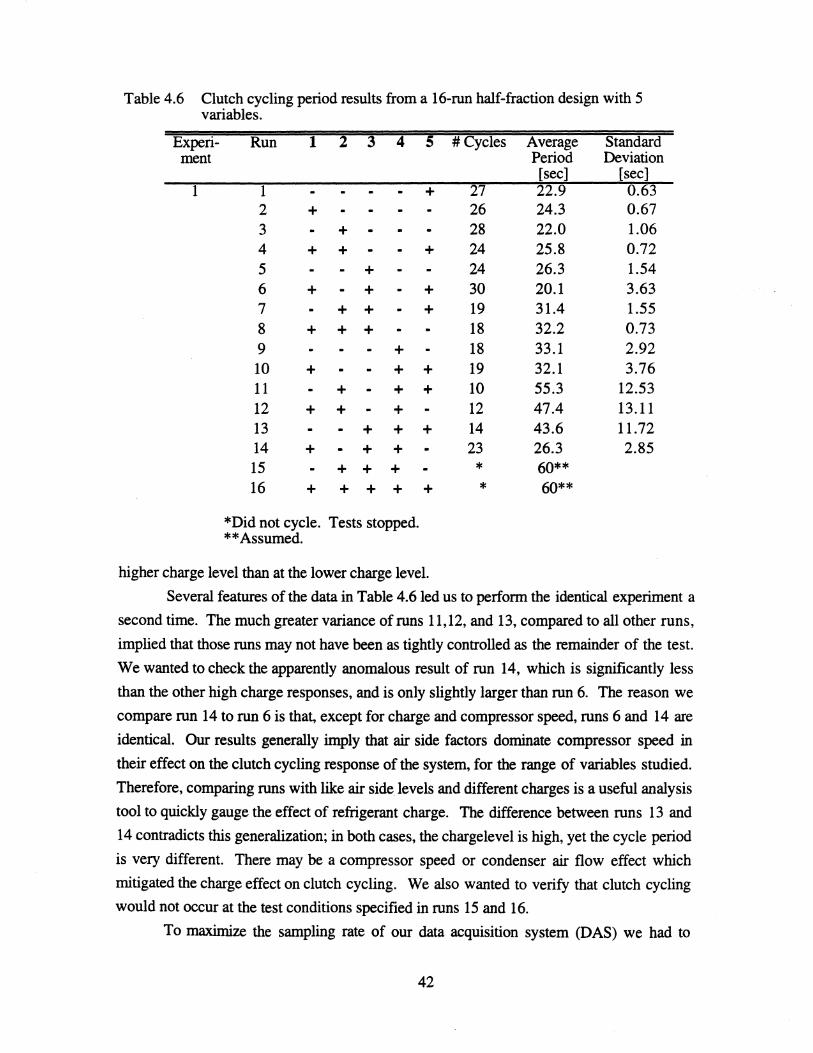
Table 4.6 Clutch cycling period results from a 16-run half-fraction design with 5 variables.

Experi-ment

1

Run 1 2 3 4

1 2 + 3 + 4 + + 5 + 6 + + 7 + + 8 + + + 9 + 10 + + 11 + + 12 + + + 13 + + 14 + + + 15 + + + 16 + + + +

*Did not cycle. Tests stopped. **Assumed.

5

+

+

+ +

+ +

+

+

higher charge level than at the lower charge level.

# Cycles Average Standard Period Deviation [sec] [sec]

27 22.9 0.63 26 24.3 0.67 28 22.0 1.06 24 25.8 0.72 24 26.3 1.54 30 20.1 3.63 19 31.4 1.55 18 32.2 0.73 18 33.1 2.92 19 32.1 3.76 10 55.3 12.53 12 47.4 13.11 14 43.6 11.72 23 26.3 2.85

* 60** * 60**

Several features of the data in Table 4.6 led us to perform the identical experiment a

second time. The much greater variance of runs 11,12, and 13, compared to all other runs,

implied that those runs may not have been as tightly controlled as the remainder of the test.

We wanted to check the apparently anomalous result of run 14, which is significantly less

than the other high charge responses, and is only slightly larger than run 6. The reason we

compare run 14 to run 6 is that, except for charge and compressor speed, runs 6 and 14 are

identical. Our results generally imply that air side factors dominate compressor speed in

their effect on the clutch cycling response of the system, for the range of variables studied.

Therefore, comparing runs with like air side levels and different charges is a useful analysis

tool to quickly gauge the effect of refrigerant charge. The difference between runs 13 and

14 contradicts this generalization; in both cases, the chargelevel is high, yet the cycle period

is very different. There may be a compressor speed or condenser air flow effect which

mitigated the charge effect on clutch cycling. We also wanted to verify that clutch cycling

would not occur at the test conditions specified in runs 15 and 16.

To maximize the sampling rate of our data acquisition system (DAS) we had to

42

disable the autozero feature of the scanning digital multimeter (DMM) which reads each

channel. We found that this introduced a ~V level error that caused, on average, a + 1.6 F

error in each thermocouple channel, some of which we display in real-time for purposes of

test control. We knew, from manufacturer's technical manuals and experimental results,

that the sensitivity of· the clutch cycling period increases with increasing temperature.

Therefore, this temperature error became very significant at higher air temperatures. We

calculated, verified and corrected this bias in our data collection, reduction and real-time

monitoring, and we also decided to run the experiment again. Table 4.7 presents the clutch

cycling period results for the second experiment.

The smaller variances in the clutch cycling response show that we improved our

control of test conditions. The data obtained show, in every case, that longer clutch cycling

periods are associated with higher charge in runs with like air side conditions. This

observation is quantified in Tables 4.8 and 4.9, in which we present the results of the

analysis of main effects and second order interactions for the first and second experiments.

Note how the responses observed in runs 13 and 14 are quite similar in the second

experiment. This observation supports our hypothesis that the first set of tests were not

sufficiently well controlled.

Table 4.7 Results from repeated 16-run half fraction design with 5 variables.

Experi- Run 1 2 3 4 5 # Cycles Average Standard ment Period Deviation

[sec] [sec] 2 1 - + 22 28.0 3.31

2 + 25 24.2 0.95 3 - + 25 24.4 3.18 4 + + - + 30 21.1 1.57 5 - + 25 24.8 1.27 6 + - + - + 27 23.0 1.31 7 - + + - + 20 29.9 4.97 8 + + + 17 32.8 1.40 9 - + 20 31.2 4.76 10 + - + + 15 39.4 0.86 11 - + - + + 17 34.6 2.50 12 + + - + 17 36.1 2.35 13 - + + + 20 30.4 3.34 14 + - + + - 20 29.9 2.47

3 15 - + + + 9 61.4 40.72 3 16 + + + + + 6 57.7 41.99

43

Table 4.8 Experiment 1: Main Effects and Interactions.

Experiment 1: Main Effects and Interactions

Mean period = 32.9, s = 11.29

1 = 1.12 2 = 9.69 3 = 6.77 4 = 14.58 5 = 0.34

12 = 0.39 13 = -2.58 14= 1.16 15 = 4.90 23 = 9.54 24 = 5.24 25 = 0.04 34 = 2.98 35 = 5.38 45 = 1.48

Table 4.9 Experiment 2: Main Effects and Interactions.

Experiment 2: Main Effects and Interactions Mean period = 33.1, s = 11.62

1 = -0.07 2 = 8.38 3 = 6.36 4 = 14.07 5 = -0.07

12 = -0.56 13 = -0.20 14 = 1.42 15 = 5.03 23 = 10.06 24 = 6.32 25 = -2.77 34 = 3.16 35 = 5.29 45 = 0.96

44

We notice that there is not a significant change, between experiments, in the

calculated mean period, or in each of the main effects or interactions. We therefore state

that the experiments were repeatable and consistent. We also notice that the largest main

effect is of factor 4, refrigerant charge. To be rigorously statistically significant, a main

effect or interaction should differ from the mean response by an amount greater than 2

sample standard deviations of the mean response. In both experiment 1 and experiment 2,

main effect 4 is roughly 1.2 times the sample standard deviation of the mean response.

From a qualitative standpoint, however, the level of refrigerant charge clearly affects

system response. We must realize that the analysis of factorial designs makes assumptions

about the smoothness and linearity of the response function. These assumptions are very

likely not applicable, in general, to the clutch cycling period. We must augment the

arithmetical statistical analysis with prior physical knowledge and engineering reasoning.

Consider Table 4.10, which ranks the main effects and interactions calculated for

experiment 2, in descending order, and explicitly tabulates the mean clutch cycling period

and standard deviation at low charge and high charge. Table 4.10 clearly illustrates the

strong effect that refrigerant charge has on clutch cycling period and the variance of the

clutch cycling period. The data imply that the clutch cycling period of this air conditioning

Table 4.10 Experiment 2: Analysis of Main Effects and Interactions.

Mean Period Std Dev all tests

low charge high charge

33.1 26.0 40.1

Main Effects Refrigerant Charge (4) 14.1

Condenser Air Inlet Temp (2) 8.4 Evaporator Air Inlet Temp (3) 6.4 Condenser Air Flow Rate (1) -0.1

Compressor Speed (5) -0.1

Interactions 23 10.06 24 6.32 35 5.29 15 5.03 34 3.16 14 1.42 45 0.96 12 -0.56 13 -0.70 25 -2.77

45

11.5 3.9 12.5

system, operating in quasi-steady state, is a reliable indicator of the relative amount of

refrigerant charge in the system.

Now consider the main effect of factors 2 and 3, condenser air inlet temperature and

evaporator air inlet temperature. Both factors exhibit noticeable main effects, and exhibit a

strong, in fact the largest, interaction. Box and Hunter [20] explain, that in the case where

a significant interaction exists, no positive statement can be made about the significance of

the corresponding main effects. The factors must be considered jointly. The physical

interpretation of this interaction is that the higher inlet temperatures raise the steady state

condensing and evaporating pressure of the refrigerant. In addition, the condenser inlet

temperature has a strong effect on the subcooling of the liquid refrigerant, due to the

narrowing of the R134a saturation dome as condensing pressure increases (see Figure

3.1). Raising either temperature independently causes the evaporating pressure to rise;

raising both temperatures causes the evaporating pressure to rise dramatically. As the

evaporating pressure rises, it takes longer for the evaporator outlet pressure to "pull down"

to the low pressure clutch cycling setpoint.

The interaction computed between compressor speed and condenser air flow rate

provided an important lesson in critical analysis of statistical data. The data show that the

main effects of compressor speed and condenser air flow rate, over the range studied, is

negligible. It appears, however, that these two factors exhibit an interaction that is much

larger than either of their main effects, although the interaction itself is not significant. This

interaction does, however, provide a good example of what we believe to be confounding

in the data. In our experiment design, the 15 interaction is confounded with the 234

interaction. We had assumed, a priori, that third order and higher interaction were

negligible. However, the 234 interaction is the combination of the most significant main

effect with the most significant interaction. We think it is more reasonable to conclude that

the combined effect of air inlet temperatures and refrigerant charge will be more significant

than the combined effect of compressor speed and condenser air flow rate. This hypothesis

should be tested by performing tests from the complementary half-fraction to the

experiment we have analyzed here and computing unconfounded second order interactions.

4.6 Clutch Cycling: Analysis of On-Cycle and Off-Cycle Behavior

4.6.1 Duty Cycle Analysis

Evaporator refrigerant temperatures and pressures are very senSItIve to charge

levels, and plots of these two variables are useful to explain charge level effects on clutch

cycling. Figure 4.4 presents an example of typical plots of the refrigerant temperature and

pressure recorded at the evaporator outlet, in this case recorded during run 2-5. The left-

46

e ! 30 ~J e ., 20 ~£

10

Run 2-5

Evaporator Refrigerant Outlet Evaporator Refrigerant Outlet

10 .•••.•.. - Tern ....•.... Tero -scal<dRPM

o~~~~~~~~~~~~~ O~~~~--~~~~~~~~

o 100 200 300 400 SOIl 600 700 300 320 340 360 380 400

time [sec] time [sec]

Figure 4.4 Run 2-5: Time history of evaporator outlet refrigerant temperature and pressure.

hand plot is the entire record of data, 600 samples gathered over about 660 seconds; the

right-hand plot is a closeup of a 100 second window.

We have previously established that the cycling period decreases with decreasing

refrigerant charge. We would like to know how this change in the cycling period is

distributed over the duty cycle shown in Figure 4.4. To answer this question, we analyzed

the duration of the "on" cycle and "off' cycle for each run. In Figure 4.4, the "on" cycle is

associated with the lower value of the scaled RPM trace (due to loading of the compressor

drive motor) and with the pulldown of evaporator outlet temperature and pressure. Table

4.11 presents the results of this analysis, over all experiment runs, for the off cycle6•

Table 4.11 shows that the off-cycle time is not strongly influenced by any factor,

Table 4.11 Analysis of Off-Cycle Time for all runs.

GrandAvg

Charge (+) Charge (-)

Tcai (+) Tcai (-)

Teai (+) Teai (-)

Charge (+ )/feai (-)

Mean StdDev 10.4 2.2

11.6 2.1 9.4 1.7

10.0 2.1 10.6 2.2

9.2 11.2

12.1

1.8 2.0

2.1

nor does it exhibit significant variance. From this observation we conclude that the

evaporator heat up times, as measured by the time it takes for the evaporator outlet pressure

to rise to the high pressure clutch cycling setpoint, are only weakly affected by the amount

6 Appendix F contains the total cycle and off-cycle data for all runs.

47

of charge in the system. We infer that the amount of refrigerant charge in the system most

strongly affects the "on" cycle. This conclusion is strongly supported by an example.

Figure 4.5 presents 100 second windows of data recorded during run 2-4 and run

2-12. These runs are identical except for charge level and compressor speed, and we have

established that compressor speed has a negligible effect on the clutch cycling period.

Evaporator Refrigerant Outlet

Run 2-4

~00~~-32~0~~34O~~~3~~~~3~80~~400

lime [sec)

Evaporator Refrigerant Outlet

Run 2-12

~ .. -.-.-, r·_··--. \ ...... _ ..... _i \ ..... _ ..... _ .. _!

10

O~~~~~~~~~~~~~

300 320 340 3~ 380 400 lime [sec)

Figure 4.5 Runs 2-4 and 2-12: Time history of evaporator outlet refrigerant temperature and pressure.

By inspection of Figure 4.5 we notice that both the on cycle and the off cycle

behavior are affected. The off cycle is about 15% longer in run 2-12 than in run 2-4, but

the on cycle is nearly twice as long. The effect of the change in refrigerant charge is

reflected almost entirely in the on cycle. We again see that the evaporator heat up transient,

during the off cycle, is minimally influenced by the amount of charge in the system. We

also see that the evaporator pulldown is strongly influenced by the charge level. Plots of all

16 runs performed in experiment 2 are located at Appendix F of this thesis.

4.6.2 Evaporator Pulldown Analysis 1

Compare the behavior of evaporator temperature and pressure, between runs 2-4

and 2-12, during each on cycle. In both cases, the refrigerant temperature and pressure

initially drop rapidly as the compressor evacuates the low pressure side of the refrigerant

loop_ In the case of run 2-4, there is insufficient refrigerant inventory in the high pressure

side of the loop to reflood the evaporator and stabilize the outlet pressure. The outlet

pressure drops rapidly to the low pressure setpoint and the compressor clutch trips. In run

2-12, there is sufficient refrigerant inventory in the high pressure side, at the end of the off

cycle, to reflood the evaporator. The compressor repressurizes the condenser, and the

mass flow rate of refrigerant through the orifice tube increases. After the initial evacuation,

the evaporator refloods and reduces the rate of change of the decrease in evaporator outlet

48

pressure.

During each on cycle, we noticed that the slope of the evaporator outlet temperature

signal exhibited a clear change. We associated this feature of the outlet temperature with

the initial pulldown and termed it the Time to Temperature Turning (TTT). We calculated

mean TTT for all runs in all experiments, and evaluated the effect of different factors on

TTT. The results are presented in Table 4.12.

Table 4.12 shows that TTT is strongly influenced by refrigerant charge, and that the

difference is statistically significant at the .01 level, if we use the low charge level as a

reference. That is, the mean TTT at high charge is different from the mean TTT at low

charge by more than 3 standard deviations of the mean TTT at low charge.

An interesting phenomenon associated with TTT is illustrated by plotting the

saturation temperature corresponding to the outlet pressure on the same axis as the outlet

temperature, as we have done in Figure 4.5. We noticed that TTT is very closely related to

the point at which the refrigerant state at the evaporator outlet changes from a high-quality,

two-phase mixture to a single-phase, slightly superheated vapor. We think this is another

manifestation of the refrigerant inventory available to reflood the evaporator at the end of

the off cycle. At lower charges, the evaporator does not reflood as quickly as at higher

charges, and the dry out point migrates upstream in the evaporator.

We have now developed two complementary methods of measuring features of the

clutch cycling transient that we can use to make diagnostic inferences about the state of

refrigerant charge in the system.

4.6.3

Table 4.12 Analysis of On-Cycle Pulldown Transient at the Evaporator Outlet.

Mean StdDev Grand avg 7.8 1.9

Charge(+) 9.2 1.9 Charge(-) 6.5 0.8

Tcai(+) 7.5 1.8 Tcai(-) 7.9 2.0

Teai(+) 7.6 1.6 Teai(-) 7.9 2.1

Evaporator Pulldown Analysis 2

Earlier, we alluded to the fact that we expected the combined effect of refrigerant

charge and air side inlet temperatures to be significant. The data of runs 3-15 and 3-16, in

49

which both air inlet temperatures and the charge were set to their high level, clearly

demonstrate this interaction. Refer again to Table 4.7 and notice that the clutch cycling

period is almost twice as long in these runs as for any other run. The period, however,

was highly irregular, as we illustrate in Figure 4.6.

The performance of the evaporator in runs 3-15 and 3-16 exhibits characteristics of

both the low charge and high charge performance of other air inlet temperature

combinations. There are isolated groups of fairly regular cycling of 20-30 seconds

duration. There are also long periods during which the evaporator outlet pressure remains

steady at just above the low pressure setpoint of 25 psig. We can relate this to an

observation we made during the charge optimization testing. Refer back to Figures 4.2 and

4.3, which present plots of evaporator temperatures versus charge and compressor speed.

Notice that at low charges the evaporator outlet refrigerant is superheated and at higher

charges it is two-phase.

At higher condenser air inlet temperatures, the enthalpy of the refrigerant in the

liquid line is higher than it is at lower condenser air inlet temperatures. We infer that the

enthalpy of the two-phase refrigerant at the inlet to the evaporator will be higher, and the

10

10

Evaporator Refrigerant Outlet

Run 3-15

100 200 300 400 500 600 700 time [sec]

Evaporator Refrigerant Outlet

-Pero ......... Tero -scaled RPM O ...................................................................................................................................... J........o.....u

o 100 200 300 400 500 600 700 time [sec]

Evaporator Refrigerant Outlet

_ ••• 1\ •••• Tero -scaledRPM o ~~~~~~~~~~~~~~

300

Run 3-16

10

320 340 360 380 time [sec]

Evaporator Refrigerant Outlet

--e--Pero ......... Tero _scaled RPM

400

o~~~~~~~~~~~~~~

300 340 380 420 460 500 time [sec]

Figure 4.6 Runs 3-15 and 3-16: Time history of evaporator outlet refrigerant temperature and pressure.

50

evaporating pressure will be higher. At higher evaporator air inlet temperatures, it is also

more difficult for the evaporator to "pull down" to a low temperature and pressure. At

higher charges, the evaporator becomes an entirely two-phase device. This fact, together

with higher condensing and evaporating pressures driven by higher air inlet temperatures,

causes the evaporator outlet pressure to remain above the low pressure cycling setpoint.

The clutch is probably tripped intermittently due to random fluctuations in the evaporator

outlet pressure when the pressure is close to the setpoint. These fluctuations are associated

with the random fluctuation in the location of the dryout point in the evaporator. This

fluctuation of the dryout point has been observed before, and was reported by Isermann

and Gruble in [43].

51

5. CONCLUSIONS

5.1 Summary of Work and Scope of Results

The goal of this project was to fonnulate a refrigerant charge loss detection scheme

for mobile air conditioning systems based on the transient behavior of directly measurable

physical variables. We studied a modified and instrumented mobile air-conditioning

system that included: a fIXed-displacement compressor equipped with a pressure cycled

clutch; an orifice tube expansion device; an accumulator; and an evaporator and a

condenser, each of which was totally enclosed in an environmentally controlled air flow

loop.

We designed a 5-factor, 2-level factorial experiment, in which we analyzed: (1) the

response of the clutch cycling period, and (2) the transient behavior of the evaporator outlet

refrigerant temperature and pressure, to changes in: refrigerant charge, compressor speed,

condenser air flow rate, condenser air inlet temperature and evaporator air inlet temperature.

We held evaporator air flow rate constant throughout the study. We simulated a narrow

range of operating conditions corresponding to a vehicle cruising at highway speeds, with

the air conditioning system operating in full recirculation mode, in a low humidity, high

ambient temperature environment. The test facility lacked the means to control humidity in

the evaporator loop, and therefore humidity was not considered in the study.

We believe that the lack of humidity control does not invalidate affect our results.

During the course of testing, the relative humidity measured in the evaporator air loop was

typically 25% to 30% at dry bulb temperatures between 60 Of and 70 Of. The dewpoint

temperatures corresponding to these conditions range from 25 Of to 37 OF. During clutch

cycling operation, the evaporator refrigerant temperature rarely fell below dew point for

more than a few seconds, and we surmised that there was little or no condensation taking

place. This conclusion is supported by humidity ratio data taken upstream and downstream

of the evaporator which shows almost zero moisture removed from the air stream. These

results can be taken as representative of behavior in an arid climate.

5.2 Conclusions

For the range of factors studied, we found that refrigerant charge exerted the

strongest influence on the total clutch cycling period. Further, we found that the on portion

of the compressor duty cycle and the Time to Temperature Turning (TTT) were highly

sensitive to the amount of refrigerant charge in the system. We found that the off portion

of the compressor duty cycle was less affected by the amount of charge. We suggest that

the clutch cycling period (or, alternatively, the on cycle time) and TTT together constitute a

basis for the detection of refrigerant charge loss in mobile air conditioning systems. We

52

found that the evaporator air inlet temperature and the condenser air inlet temperature exert a

strong combined effect on the total clutch cycling period, and we suggest that these

temperatures would have to be sensed, as well.

We found that, over the range of factors studied, compressor speed and condenser

air flow rate had virtually no effect on the measured responses. We qualify this remark by

suggesting that experiments be performed from which unconfounded second order

interactions can be computed.

We found that the evaporator air side instrumentation is satisfactory. We found that

the condenser air side instrumenatation reflects a systematic bias that is related both to air

temperature and air flow rate measurement. We clearly showed that the relatively small air

side differential temperature across the condenser, coupled with the bias in the air side

outlet temperature measurement, as currently installed, together severely limit the minimum

uncertainty acheivable in the energy balance calculation.

5.3 Recommendations and Future Work We noted earlier that a .052" diameter orifice tube was installed during the course of

testing. The orifice tube specified for use with the system components as they are installed

in a vehicle is .057" diameter. We also noted that humidity was not considered in the

study. Tests should be performed with the larger orifice tube and with evaporator air

humidity control, and the results checked against the data reported in this thesis. The

optimum charge will need to be determined with the larger orifice tube installed, and with

40% relative humidity set in the evaporator loop.

Fractional factorial type experiments are highly recommended to efficiently develop

experimental data documenting the effect of simultaneous changes in multiple variables on

mobile air conditioner performance. In particular, adding humidity as a factor brings the

total number of variable parameters in the test facility, including evaporator air flow rate, to

7. 128 runs are required to perform a full factorial, 2-1evel experiment with 7 factors. This

large matrix can be broken down into fractions which, by themselves, constitute complete

factorial designs in fewer factors. Performing the larger experiment in smaller, full

factorial "modules" is a powerful technique further discussed in [20].

It would be prudent to check the Validity of the conclusion that compressor speed

and condenser air flow rate have a negligible effect on the clutch cyclng period, over the

operating range we studied. All or part of the complementary half-fraction of the

experiment reported in Section 4 can be generated by running each test with the opposite

compressor speed.

It is apparent that the distribution of charge in the system is a key parameter. It may

be beneficial to concentrate some future work on obtaining accurate experimental

53

descriptions of the distribution of charge in the system in steady state and transient

operation. The liquid level in the accumulator could be observed by installing a vertical

sight glass on the accumulator. Detailed observations of the refrigerant flow should be

made and correlated with clutch engagement and time. A more difficult problem is

measuring the mass of refrigerant in each heat exchanger at any given time. One possible

method for accomplishing this task is illustrated by Figure 5.1. We show a heat exchanger

(either the condenser or the evaporator) that can be isolated from the remainder of the

refrigerant system by two remotely operated solenoid valves. The isolation valves shown

should be installed as close as possible to the inlet and outlet stub tubes of the heat

exchanger. The valve solenoid actuators would be controlled by a relay ouptut on the PLC

that would be controlled from the Custom Data Display. A safety interlock which opens

the compressor clutch relay output when the valve solenoid relay output is shut is

recommended. A bleed valve is shown installed in the system piping upstream of the outlet

isolation valve. The bleed valve can be located at the inlet or the outlet of the heat

exchanger, whichever is more convenient. The only requirement is that it be located on the

heat exchanger side of the isolation valves. A clean, evacuated refrigerant cylinder

immersed in an ice bath is used to collect refrigerant trapped in the heat exchanger. The

mass of trapped refrigerant is found by weighing the cylinder before and after collecting the

refrigerant. The refrigerant may be returned to the loop by the standard refrigerant charging

technique.

Evacuated cylinder -----.,..

Ice bath

Figure 5.1 A scheme for measuring the mass of refrigerant in a heat exchanger.

54

List of References [1] R. Isennann, "Model Based Fault Detection and Diagnosis Methods," presented at

Proceedings of the American Control Conference, Seattle, Washington, 1995.

[2] J. R. Rubio-Quero, "A Facility for Transient Testing of Mobile Air Conditioning Systems," M.S. Thesis, University of illinois, 1995.

[3] P. G. Weston, "Design and Construction of a Mobile Air Conditioning System Test Facility for Transient Studies," M.S.Thesis, University of illinois, 1996.

[4] J. J. Gertler, "Survey of Model-Based Failure Detection and Isolation in Complex Plants," in IEEE Control Systems, vol. December, 1988, pp. 3-11.

[5] J. Gertler, "Diagnosing Parametric Faults: From Parameter Estimation to Parity Relations," presented at Proceeedings of the American Control Conference, Seattle, Washington, 1995 .

. [6] R. Isennann, "Process Fault Detection Based on ModeliD.g and Estimation Methods -A Survey," Automatica, vol. 20, pp. 387-404, 1984.

[7] R. Isennann and B. Freyennuth, "Process Fault Diagnosis Based on Process Model Knowledge - Part I: Principles for Fault Diagnosis with Parameter Estimation," ASME Journal of Dynamic Systems, Measurement and Control, vol. 113, pp. 620-626, 1991.

[8] R. Isennann and B. Freyennuth, "Process Fault Diagnosis Based on Process Model Knowledge - Part IT: Case Study Experiments," ASME Journal of Dynamic Systems, Measurement and Control, vol. 113, pp. 637-633, 1991.

[9] R. Isennann, "Fault Diagnosis of Machines via Parameter Estimation and Knowledge Processing - Tutorial Paper," Automatica, vol. 29, pp. 815-835, 1993.

[10] W. S. Lee, D. L. Grosh, F. A. Tillman, and C. H. Lie, "Fault Tree Analysis, Methods, and Applications - A Review," IEEE Transactions on Reliabilty, vol. R-34, pp. 194-203, 1985.

[11] Y. E. Faitakis and J. C. Kantor, "Residual based fault detection using an output observer," presented at Proceedings of the American Control Conference, Seattle, Washington, 1995.

[12] P. S. Fasolo and D. E. Seborg, "Monitoring and Fault Detection for an HV AC Control System," HVAC&R Research, vol. 1, pp. 177-193, 1995.

[13] H. T. Grimmelius, J. K. Woud, and G. Been, "On-line failure diagnosis for compression refrigeration plants," Int. Journal of Refrigeration, vol. 18, pp. 31-41, 1995.

[14] H. Inatsu, H. Matsuo, et. al., "Development of Refrigerant Monitoring System for Automotive Air-Conditioning System," SAE Transactions, vol. 101, pp. 29-37, 1992.

[15] T. Pfeufer and T. Holling, "Model-Based Fault Detection for Time-Variant Processes with Application to and Automotive Actuator," presented at Proceedings of the American Control Conference, Seattle, Washington, 1995.

[16] T. M. Rossi and J. E. Braun, "Using Thennodynamic Impact for Detecting Refrigerant Leaks in Vapor Compression Equipment," presented at Proceedings of the American Control Conference, ~eattle, Washington, 1995.

[17] T. Sorsa and H. N. Koivo, "Application of Artificial Neural Networks in Process Fault Diagnosis," Automatica, vol. 29, pp. 843-849, 1993.

55

[18] K. Fukunaga, Introduction to Statistical Pattern Recognition, 2 ed. San Diego: Academic Press, 1990.

[19] "AlC Refrigerant Systems Reference Manual," Confidential.

[20] G. E. P. Box, W. G. Hunter, and J. S. Hunter, Statistics for Experimenters: John Wiley & Sons, 1978.

[21] L. L. Lapin, Probability and Statistics for Modem Engineering. Belmont, California: PWS Publishers, 1983.

[22] I. Miller and J. E. Freund, Probability and Statistics for Engineers, 3rd ed. Englewood Cliffs, New Jersey: Prentice-Hall, Inc., 1985.

[23]ASHRAE Handbook of Fundmnentals IP Edition, 1993. Atlanta, GA.: American Society of Heating, Refrigeration and Air Conditioning Engineers.

[24] W. F. Stoecker and J. W. Jones, Refrigeration and Air Conditioning: McGraw-Hill, 1982.

[25] M. Farzad, "Modeling the Effects of Refrigerant Charging on Air Conditioner Perfonnance Characteristics for Three Expansion Devices," Ph.D. Thesis, Texas A&M University, 1990.

[26] M. Tanino, T. Takano, and H. Sakamoto, "Damage Modes and Protective System for an Automobile Cooler Cycle," SAE Transactions, vol. 96, pp. 1.107-1.116, 1988.

[27] T. A. Micheal, "Design of an Automotive Air Conditioning Test Stand for Screening and Transient Studies," M.S. Thesis, University of lllinois, 1989.

[28] M. K. Heun, "Perfonnance and Optimization of Microchannel Condensers," Ph.D. Thesis, University of lllinois, 1995.

[29] E. O. Doebelin, Measurement Systems: Application and Design, 4th ed: McGraw-Hill, Inc., 1990.

[30] D. M. Staley, C. W. Bullard, and R. R. Crawford, "Steady-State Perfonnance of a Domestic RefrigeratorlFreezer Using R12 and R134a," ACRC TR-22, University of lllinois, 1992.

[31] R. P. Benedict, Fundamentals of Temperature, Pressure and Flow Measurement, 3rd ed. New York: Wiley, 1984.

[32] Using the HP-IB Interface with Microsoft Windows: Hewlett-Packard, 1991.

[33] Using the HP-IB Interface and Command Library with DOS: Hewlett-Packard, 1991.

[34]HP 75000 Series BIC: 5 112-Digit Multimeter HP 1326B1E1411B Users Manual: Hewlett-Packard, 1994.

[35]HP 75000 Family ofVXI Products and Services Catalog: Hewlett-Packard, 1995.

[36] R. Helsel, Cutting Your Test Development Time with HP -VEE. Englewood Cliffs, NJ: Prentice-Hall, 1994.

[37] HP Standard Instrument Control Library for Windows: Hewlett-Packard, 1994.

[38] HP Standard Instrument Control Library Reference Manual: Hewlett-Packard, 1995.

[39] SLC 500 Analog 110 Modules User Manual: Allen-Bradley, 1994.

[40] Rockwell Software PLC-500 A.I. Series Ladder Logistics Software Reference: ICOM, Inc., 1992.

56

[41] Rockwell Software PLC-500 A.I.Series Ladder Logistics Processor Reference: ICOM,1992.

[42] SLC500 and Micrologix 1000 Instruction Set: Allen-Bradley, 1995.

[43] W.-D. Gruhle and R. Isennann, "Modeling and Control of a Refrigerant Evaporator," ASME Journal of Dynamic Systems, Measurement and Control, vol. 107, pp. 235-240, 1985.

[44] Toshiba TOSVERT VF-SX Compact Inverter Instruction Manual, 1992.

[45] "Yaskawa Electric Varispeed-616GII Instruction Manual," , 1988.

57

Appendix A. Pressure Transducer Calibration Calibrations of the liquid line venturi and compressor suction gage pressure

transducers, and two-point calibration checks of the compressor discharge and condenser

inlet gage pressure transducers are reported in this section. The evaporator outlet gage

pressure transducer calibration and aero point were checked by inspection, did not require

adjustment, and so are not reported here.

58

Liquid Line Venturi Gage Pressure Transducer Calibration Type: Setra 207 SerialNumber: 253459 Range: 0-500 psig Output: 0.1 V -5.1 V DC Excitation: 24 VDC Date: 29-Sep-95

EsiS Volts ~uEl Volts ~downl 15.95 0.2700 0.2560 50.76 0.6019 0.6020

100.07 1.0907 1.0905 150.83 1.5930 1.5935 200.14 2.0810 2.0820 250.91 2.5820 2.5830 300.22 3.0700 3.0720 350.98 3.5720 3.5730 390.14 3.9600

I SloEe = 101.15 EsiSN I

Plv Calibration

400 -

300

bIl .;ji 200

: Q..

psig = lOU5v - 10.351 R2 = 1

o ~.---------+--------~------------------~ o 2

volts 3 4

Figure A.I Liquid Line Venturi Inlet Gage Pressure Transducer Calibration

59

Compressor Suction Gage Pressure Transducer Calibration Type: Setra 207 SerialNumber: 270489 Range: 0-100 psig Output: 0.lV-5.1V DC Excitation: 24VDC Date: 3-Oct-95

Esi~ Volts !uE~ Volts !down~ 0.00 0.1884 0.1855 5.08 0.4382 0.44

10.01 0.6855 0.6868 15.08 0.9392 0.9407 20.01 1.186 1.187 25.09 1.439 1.44 30.02 1.6854 1.686 35.10 1.9385 1.9386 39.01 2.1335 20.30 1.1985 1.199 30.46 1.7025 1.706 40.61 2.2124 2.21 50.76 2.7167 2.715 60.91 3.2234 3.223 69.61 3.652 3.654 79.77 4.158

I SloEe=20.084 EsigN

Pkri Calibration

80

70

60

50

psig = 20.084v - 3.7942 /~ R2= 1 /

20 + 10 ~

" ,/

~

, ., .,,'

/'

~

" .I /

/ ~

/

o ~----~--------------~------------o 2 3 4 5

volts

Figure A.2 Compressor Suction Gage Pressure Transducer Calibration

60

Table A.t Compressor Discharge Pressure Transducer Calibration Check

Compressor Discharge Gage Pressure Transducer Calibration Check Type: Setra 207 SeriaINumber: 202281 Range: 0-500psig Output: 0.1 - 5.1 V Excitation: Date:

24V 10-0ct-95

Two-point calibration check: Voltage output set to 0.1021 V when vented (0 psig); Pressurized calibration standard is calibrated Liquid Venturi pressure transducer reading.

psig Volts o 0.1021

74.28 0.7191

IS10pe=120.39 psigN

Table A.2 Condenser Inlet Pressure Transducer Calibration Check

Condenser Inlet Gage Pressure Transducer Calibration Check Type: Setra 207 SeriaINumber: 253458 Range: 0-500psig Output: 0.1 - 5.1V Excitation: Date:

24 V 10-0ct-95

Two-point calibration check: Voltage output set to 0.1023 V when vented (0 psig); Pressurized calibration standard is calibrated Liquid Venturi pressure transducer reading.

psig Volts o 0.1023

195 2.0470

I Slope=100.27 psigN

61

Appendix B. Zone Box Diagrams

62

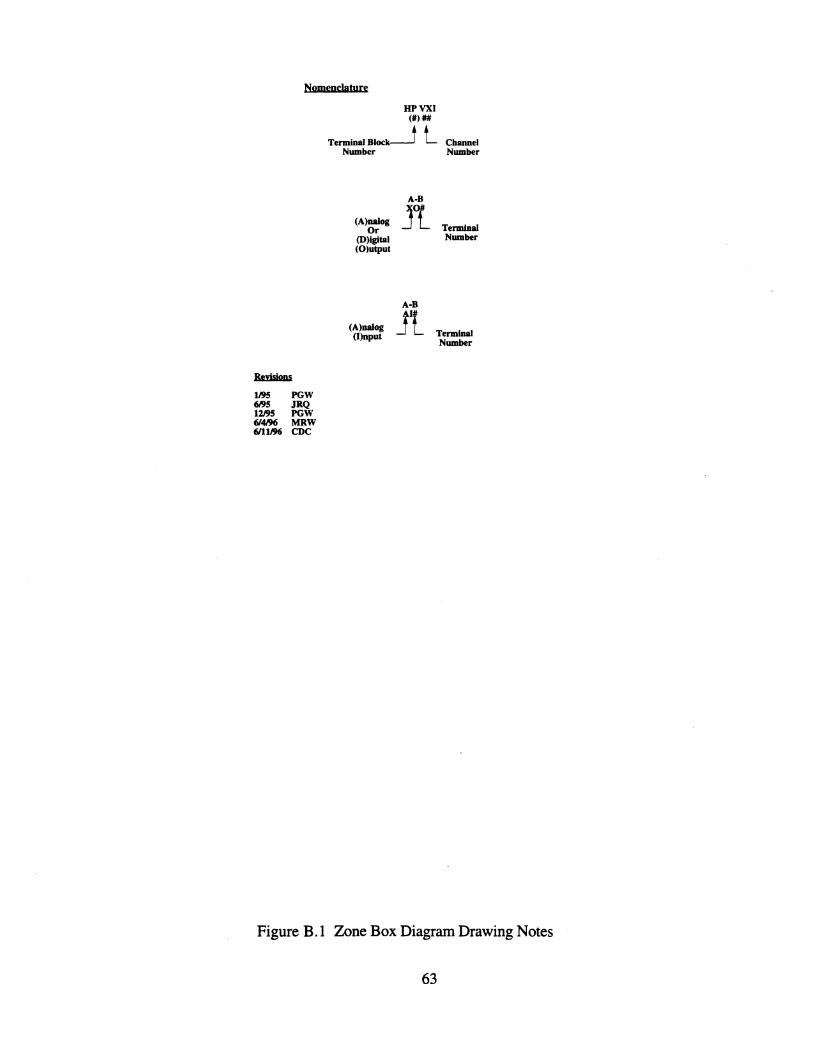
Nomenclature

Ik!iIiIIDi

1I9S PGW 6I9S JRQ 1219S PGW 6/4/96 MRW 6/11J% CDC

HPVXI (#)##

Terminal BIOCk~ L Number

Cbannel Number

(A)naJog Or

(D)igItal (O)utput

(A)naJog (I)nput

A·B

Jt

A·B

Jt

Terminal Number

Terminal Number

Figure B.t Zone Box Diagram Drawing Notes

63

Power Supply Rail

.I-J!!l~--+-o Term CC

.j....l::!!-_-+-o Term Ground

CondHeater Set Point

.j...!!:!!!-_-+-O Term ST Motor Safety SlOP

TermCC

+S Volt Power Supply

Figure B.2 Condenser Loop Zone Box Diagram

64

Teri Cu

Co C

lbath Cu

Tero Cu

Co C

lbath HPVXI Cu (3)03

Ten Cu

Co C

lbath HPVXI Cu (3)06

Cu n Tcro <II CO

Thath C Cu

Tkri Cu

Co

lbath C Cu

Tkro Cu

Co

lbath C Cu

Tlv Cu

Co

Thath C Cu

Toll Cu

Co

lbath C Cu

+S Volt Power Supply

Figure B.3 Refrigerant System Zone Box Diagram

65

Inlet Thermocouple Grid. Teal

Teao

Tbath

Teav

Thath

(48 ptgrld)

Power Supply Rail

Figure B.4 Evaporator Loop Zone Box Diagram (1 of 2)

66

RHeao " TRHeao

R ... Mod I ...&X ILl: E Z .... 80 IIII.:&... I E 81 yap c: tmll er owcrAQ

VDC ~ red , red TermF Start

A-B I Forward 002 OUT 11 hlk 'tlk TermCC

elr elr Term Ground

red 'wht TermST

A-B VDC W~I Motor

I I blk 'gm Safety Stop

OUT TermCC

Camp MIIlIU: Qmtmlkl:

Wire #19 red' wht

A-B I~ I 11 blk1;gm

Term 1

002 OUT Term 11

Term 12 elr elr

Figure B.S Evaporator Loop Zone Box Diagram (2 of 2)

67

Table B.l Data Acquisition System Channel Cross Reference

HP DAS Rewiring (Completed 5/29/96) OLD NEW

Name Bundle Range [V] IVXI ChanneIMUX·CH VXI ChanneIMUX··CH V_Teri R-l 0.125 0 1-0 0 1--0 V_Tero R-2 0.125 1 1-1 1 1--1 V_Tkri R-5 0.125 4 1-4 2 1--2 V_Tkro R-6 0.125 5 1-5 3 1--3 V_Tcri R-3 0.125 2 1-2 4 1--4 V_Tcro R-4 0.125 3 1-3 5 1--5 V_Tlv R-7 0.125 6 1-6 6 1--6 V_Teai E-l 0.125 32 3-0 7 1--7 V_Teao E-2 0.125 33 3-1 8 1--8 V_Teav E-3 0.125 34 3-2 9 1--9 V_Tcai C-l 0.125 16 2-0 lO l--lO V_Tcao C-2 0.125 17 2-1 11 1--11 V_Tcav C-3 0.125 18 2-2 12 1--12

Toil R-8 0.125 7 1-7 13 1--13 V_dPdv R-16 0.125 15 1-15 16 2--0 V_dPlv R-17 0.125 28 2-12 17 2--1 A_micro C-6 0.125 21 2-5 18 2--2 A_dPeav E-5 0.125 36 3-4 19 2--3 A_dPcav C-5 0.125 20 2-4 20 2--4

Oil C-11 0.125 25 2-9 21 2--5 TRHeai E-7 8 37 3-5 24 2--8 TRHeao E-lO 8 39 3-7 25 2--9 TRHcao C-8 8 22 2-6 26 2--10 RHeai E-8 8 38 3-6 27 2--11 RHeao E-11 8 40 3-8 28 2--12 RHcao C-9 8 23 2-7 29 2--13

TmstcVolt R-19 8 30 2-14 30 2--14 V_dPer R-14 8 13 1-13 32 3--0 V_Pero R-9 8 8 1-8 33 3--1 V_Pkri R-11 8 10 l-lO 34 3--2 V_Pkro R-12 8 11 1-11 35 3--3 V_Pcri R-lO 8 9 1-9 36 3--4 V_dPcr R-15 8 14 1-14 37 3--5 V_Plv R-13 8 12 1-12 38 3--6

V_Peav E-4 8 35 3-3 39 3--7 V_Pcav C-4 8 19 2-3 40 3--8

drpm E-12 8 41 3-9 41 3--9 dtorque E-13 8 42 3-lO 42 3--10

Five Volts R-18 8 29 2-13 43 3--11

68

Appendix C. Programmable Logic Controller System We use an Allen-Bradley SLC-500 Programmable Logic Controller (PLC) system

to control the three inverters and the compressor clutch circuit described in Section 4. This

Appendix presents a brief discussion of PLC-to-inverter wiring interconnections and an

annotated listing of the ladder logic program used to execute the transient and steady-state

tests reported in this study .

. Remote Operation of Inverters

The inverters are wired for remote start-stop control and remote setting of drive

frequency. The Zone Box Diagrams, Figures B.2, B.4 and B.5 herein, schematically

depict the required wiring configurations. For the Toshiba inverters, compare these

diagrams with wiring example 4 on page 6-2 of [44]. Notice that we have configured these

controllers for forward run only by wiring relay outputs across terminals ST, F and CC,

but not terminal R. For the PoWrMaster inverter compare with Figure 5 on page 7 of [45].

PLC Overview

The PLC system consists of the PLC modules, chassis and wiring interconnections

with external devices; a personal computer tennina1; and programming software. We will .

now consider PLC concepts and their application in this project. This discussion is not

intended to serve as a stand-alone reference for PLC programming or operations.

References [39-42] should be reviewed concurrently with the reading of this Appendix.

The PLC is programmed using a concept called ladder logic. Ladder logic

describes both the conceptual structure and the physical representation of the program,

which is that of a sequence of rungs of a ladder. The processor scans each rung of a

program, beginning with the first rung and proceeding in sequence, and performs the

instructions on each rung from left to right. In general, each rung terminates with an output

instruction which changes the value of a memory location in the PLC processor. Preceding

each rung output may be one or several instructions which can assume one of two values:

logical FALSE or logical TRUE. When all the instructions on a rung are TRUE, the output

instruction is executed. A rung may include only an output instruction; in this case, the

rung output is executed each time the processor reaches that particular rung. Logical

branching instructions permit the programmer to modify the default top-down sequencing

routine.

Every input and output terminal on each 110 module installed in the PLC chassis is

assigned a unique, permanent memory location in the PLC processor. Relay (or digital

logic) outputs and inputs are normally open and are assigned to single bits. If the bit is

TRUE (1), the relay output shuts; if the bit is FALSE (0), the relay output is open. Analog

69

outputs and inputs are assigned to 16-bit words.

The programmer writes or edits the ladder logic program with the PLC on- or

off-line. To implement the program, the PLC is placed off-line, the program is

downloaded to the PLC processor, and then the PLC is placed back on-line. The program

executes continuously and autonomously as long as the PLC processor is energized,

on-line, and as long as there is no fault condition which causes the PLC processor to stop

execution.

The remainder of this Appendix contains a report which was generated using the

PLC-500 Ladder Logistics software. The remarks are keyed to the me name and Report

page number listed in the file header on each page.

70

Pale o 1 2

3

Name Table of Contents Program File List File #2 MAIN Proj:CLUCYC

File #3: CYCLE Proj:CLUCYC

Rlm& Description

o Examine bit 2 in Bit File B3 (variable name: CLU_CYC_ENA). If bit 2 is TRUE (1), then Jump to Clutch Cycling Routine.

1 Examine bit 3 in Bit File B3 (variable name: SPD_CHNG). If bit 3 is TRUE (1), then Jump to Motor Speed Change Routine. Note: Bit 2 and Bit 3 are set interactively by the user at the PC terminal via the Custom Data Display.

o Enter Subroutine. Examine bit 1 in Bit File B3 (variable name: CHNG_LIM). Ifbit 1 is TRUE (1), then Jump to Clutch Cycling Pressure Limit Conversion Routine. Note: Bit 1 is set interactively by the user at the PC terminal via the Custom Data Display.

1 If the value at source A (memory location I: 1.0, variable name P _K_R_CSIG) is less than or equal to the value at source B (memory location NlO:5),then . the instruction is TRUE, and bit 0 in Bit File B3 will be "latched" (set to TRUE; can be set to FALSE only with an "unlatch" instruction). This rung latches bit 0 if the evaporator refrigerant is greater than or equal to the high pressure setpoint. Note: 1:1.0 is the 16-bit integer value (decimal) obtained from the AID conversion of analog input Channel O. This input is connected to the output of the evaporator refrigerant outler pressure transducer. Note: NlO:5 stores the scaled integer value corresponding to the high pressure setpoint. During testing, the pressure setpoint was 43 psig, which corresponded to a value in NlO:5 of 7200.

2 If the value at Source A (memory location I: 1.0) is less than the value at Source B (memory location NlO:6), then the instruction is TRUE, and bit 0 in Bit File B3 is ''unlatched.'; This rung unlatches bit 0 if the evaporator refrigerant pressure is less than the low pressure setpoint. Note: NlO.6 stores the scaled integer value corresponding to the low pressure setpoint. During testing, the pressure setpoint was 25 psig, which corresponded to a valued in NlO:6 of 4320.

3 Examine bit 0 in Bit File 3. If TRUE, then set bit 0 in output file 0:3.0 to TRUE. Note: Output 0:3.0 corresponds to the relay output module. 0:3.0/0 corresponds to channel 0, the clutch

71

~ Name

4

5

6

7

File #4 LIM_CON Proj: CLUCYC

File #4 LIM_CON Proj: CLUCYC

File #5 SPD_CON PROJ: CLUCYC

RunK Description

o

control circuit relay. OX8 is the designator for the relay output module.

Enter Subroutine. This subroutine calculates the scaled integer value (in AID counts) which corresponds to the low-pressure setpoint entered (in psig) by the operator into memory location N7:0 in the Custom Data Display. We calculate the integer value according to the formula

where

I = 32768 P+ b 10 m

I = integer counts P = pressure setpoint (psig) b = gage pressure corresponding to 0 psig

transducer voltage (approx 0.1 V). This ensures that the 0 psig setpoint has an integer count value corresponding to 0.1 V.

m = transducer calibration slope (psiglcount).

The scale instruction adds the offset, b, represented as 21200/10000, to the setpoint, 43, and stores the result, 45 (psig).

1 The divide instruction calculates the number of counts per psig. Because of overflow limitations this value is intially calculated as

32768 1 m=

10 (10)(20.03)

2 The multiply instruction cancels the extra factor of 10 from the previous instruction.

3 The multiply instruction multiplies the corrected pressure by the slope in counts per psig to obtain the high pressure setpoint.

4-7 This page is analogous to the the previous page. The low pressure integer setpoint is calculated and stored.

8 Bit 1 in Bit File B# is unlatched. The Custom Data Display updates to show this bit is OFF.

9 Subroutine ends. Control returned to File #3 CYCLE, rung O.

o Enter inverter speed signal subroutine. Inverter speed signal requests are made by the operator in the Custom Data Display. A valid request is a 3-digit

72

Pa&e Name Run& Description decimal integer (units: 0.1 Hz) which obey s the rule

R = Sx10 where

R = speed request integer S = desired speed (smallest increment of 0.1

Hz). For example, a request of 543 represents a desired speed of 54.3 Hz. Memory location N7:3 stores the speed request for the condenser inverter. We determined the offset by trial and error. The offset is used for fine calibration of the speed request at the PLC against the speed output of the inverter.

1 The multiply instruction converts the speed request integer to analog counts, andplaces the count value in location 0:2.0. This value is converted to an analog rnA signal (14-bit resolution) and placed on analog output channelO.

2-3 Analogous to rungs 0-1, for the evaporator inverter. Speed request is set in the Custom Data Display and stored in N7:2.

8 File #5 SPD_CON 4-6 Arithmetic for calculating digital counts Proj:CLUCYC corresponding to compressor speed request in

location N7:4.

7 Unlatches bit 3 of Bit File B3.

8 Exit subroutine. Returns to Main, Rung 1.

9 Data Table File List Lists file types, abbreviations and sizes.

10 Data Base Form Lists memory locations, and default and operator assigned tags. Notice file 0:2 (analog outputs), 0:3, (relay outputs), and 1:1.0 (analog input).

11 Data Base Form Notice Bit File 3 elements, and integer files N7 and NlO.

73

PLC-SOO LAOOER LOOISTICS Report header (c) ICDI In:. 191P-1~ Program File List

LhiVersity of III irois - UrtJre Program File List Page:00lJ1

Nu!tler of Program Fi les:6

Hare Fi le Slb-Progran DescriptiCl'l

MAIN CYCLE LIM a:w SPD:a:w

o [SYSTEM DATA ST~ lEADER] 1 [RESERVED AREAl 2 Main CCI'ltrol Program 3 Main Clutch eyel irg Program 4 Ca'1I.-'erts Clutch eye l ; rg Presst.re Limi ts 5 Ca'1I.-'erts Motor Speeds

74

16: 12 06/12/96

PLC-500 LADDER LOOISTICS Report header (c) ICD'I Inc. 19fP-1994 SLC-500 Lact2r Listiflj

lkIiwrsity of III il1)is - Urbn! Fi le tfe. MAIN Proj :cw:YC Page:1XXX>2 16:12 06/1Z1%

Ersble Clutch Clutch C')<cl iflj C')<cl iflj Rcutine CLU CYC ENA CCR - a3 SR

0 JUJp To 9brcutine 2 SBR File NudJer U:3

Motor 5p!ed Motor 5p!ed 0vqec:I Flag D1IIlIe Rcutine SPO_CINi MSC

B3 JUJp To 9brcutine

3 SBR File NudJer U:5

2 [EN)]

75

PLC-SOO LADDER UXiISTICS Report hea:ler (c) leD! Ire. 1~19'i1'+ SLC-SOO Lactler Listilll

Lhi vers i ty of III i roi s - UrbEna Fi le #3 CYCLE Proj :CLLtYC Page:OOXl3

Clutch Cyt:l illl Rout ire IllcrEled Limi ts cx:R CHNG_LlM

O~ire I I~ I 11

Pieri Irp.rt: Si9. P K R I SIG -;:;,n--

1 Grtr Thin or Eql (A>~) SWrce A 1:1.0

5000 Source B N10:5

0

PIeri Irp.rt: Si9. P K R I SIG --1-";::- -

2 Less ThIn (A<B) Source A 1:1.0

5000 SaJrce B N10:6

0

Pressure Risilll or Fall illl Irdicator PRSRI FAL

- -83 3 I

0

4

76

16:12 06/12.1%

Clutch Cyt:l illl PresSlr'e Limi t CcrNersiCl'l Rout ire LCR

SR Jurp To SU:lrout

lSBR File Number

PresSlr'e R or Fall illl I rdi cator PRSRI FAL

- -83 JL

0

ire U:4

isire

PresSlr'e R i silll or Fallilll Irdicator FRS RI FAL

- -83 U' 0

Clutch CLUTCH

QVOff

o 0:3. (

0 ()(8

[EN)]

PLC-500 l.AOOER LCXiISTICS Report hea:Er (c) HXM Ire. 1S6C}-19i14 SLC-SOO Lact:ler Listil'll

li'li \IerS i ty of III i roi s - UrbEna File #4 LIM_(X)I Proj:cw:YC Page:CXXXJ4

Clutch Cycl ii'll Pres5I.I"e Limi t CcnIIers i en Routine LCR

o H 9.broutine I I

,

2

3

77

16: 12 06/121%

Press. Ga'1vrs. Tmp. Var. , P_(X)IV_TMP_' r-SCL Scale t-Scurce N10:1

21563 Rate [/10000] 1 Offset N7:0

45 Dest N10:2

14560

Press. Ccnv. Tenp. Var. 2 P (X)IV _ TMP 2 ;nI -Divide Scurce A 32768.0 Scurce B N10:0

2003 Dest N10:3

0

Press. Ccnv. Tenp. Var. 3 P (X)IV TMP 3 - ..Mn- -folIltiply Sa.rce A N10:3

0 So.Jrce B 10 Dest N10:4

0

Hig, Press. Integer HI PRESS_INT

:Mn folILtiply Sa.rce A N10:2

14560 Sa.rce B N10:4

0 Dest N10:5

0

PLC-SOO LADDER LCllISTICS Report heeder (c) ICCM Ire. 1989-1994 SLC-SOO Lad:ier Listil1l

U1i\lel'Sity of III irois - UrtB1a File #4 L1M-'DJ Proj:cw::YC Page:OOXl5 16: 12 06/12/%

Press. CcrM's. T EIIP. Var. 1 P a:w TMP 1 -.J:n- -

4f---------------------------------------------------~&ale r SCU"ce N10:1

21563 Rate [f100Xl] 1 Offset N7:1

25 Dest N10:2

Press. CcrIII. T EIIP. Var. 2 P a:w TMP 2 ~I- -

14560

5f-------------------------------------------------~Divi~ SCU"ce A SCU"ce B

Dest

32768.0 N10:0 2003

N10:3 o

Press. CcrIII. T EIIP. Var. 3 P a:w TMP 3 -..JIM - -

6f----------------------------------------------------jltJl tiply r Source A N10:3

o SCU"ce B 10 Dest N10:4

La.I Press. Integer LO PRESS INT

:"6 -

o

7 f----------------------------------------------------IItJl tiply Source A N10:2

14560 SCU"ce B N10:4

o Dest N10:6

o

78

PLC-SOO LADDER l.OOlSTICS Rep:x-t hes:Jer (c) lID! In::. 19B9-191i11t SLC-SOO La.:i:Er L istirg

Lhiversity of III irois - Urb!re Fit e #14 LIM _ (X)I Pro j :cw:YC Page:<XXXl6 16: 12 QS/12/%

Olcrged Limits ClWG LIM

- B3

8r-----------------------------------------------------~IUr_--~ 1

9r--------------------------------------------------------WVl

79

PLC-SOO LAOOER LCXiISTICS Report hea:ler (c) ICXJol In::. 1~-1994 SLC-SOO La:i:ler L istil'll

lhiwrsity of Il L irois - UrbEna File #5 SPD_CDl Proj:CLIXYC Page:00))7 16:12 1:6/12/96

Motor Speed Ccn:ienser Speed Chcr'ge Rcut i ne Tnp. Var. MSC CDl SPD 1W

O~ine I ,5cL -

I ScaLe t--Sarce N7:3

4(lI

Rate [f11XOOJ 100)) Offset -5 Dest N10:8

0

Ccn:ienser Speed Si!JlBL CDl SPD SIG

jiA -

1 ItJL tipLy Source A N10:8

0 Sarce B 52 Dest 0:2_0

12740

Evaporator Speed Tnp. Var. EVA SPD 1W

2 ,5cL -ScaLe t--Source N7:2

425 Rate [f11XOOJ 100)) Offset 200 Dest N10:7

0

Evaporator Speed Si!JlB L EVA SPD SIG

...MI -3 ItJL tipLy

Sarce A N10:7 0

Source B 30 Dest 0:2.2

19740

80

PLC-SOO LADDER LOOISTICS Report header (c) ICD! Ire. 1989-1~ SLC-SOO Lcd:ler Listilll

ltIiversity of Illirois - Urbana File tfj SPOJDI Proj:cw::YC page:CXXX!l 16:12 Q!,/12/%

Cmpressor Speed Top. Var. CD! SPO 1W ..My -.

41---------------------------------------------------fltJl tiply I-Source A N7:4

199 Source B 41 Oest N10:9

Cmpressor Speed Top. Var. CD! SPO 1W m.-

o

5~----------------------------------------------4~le Source N7:4

199 Rate U1(XXXJ] 6100 Offset N10:9

o Oest N10:9

Cmpressor Speed Si 9'1B l CD! SPO SIG

AN'I -

o

6~------------------------------------------------~~ r Source A N10:9

o Source B 6242 Oest 0:2.1

2!Bl2

Motor Speed CI1alled Flag SPO ClING

- B3

7r-----------------------------------------------<Ur---3

81--------------------------------------------------------~]-

81

PLC-SOO LAOOER LOOISTICS Report hes:ier (c) ICIJol In::. 1969-1994 Data TabLe File List

Lhiversity of Il Lirois - Urbena Data Table Fi le List Page:1XKXl9

Nu1tler of Data FiLes:11

Nare Descripticn File T}'pe Mode Size:ELEIIS

0 0 Q.ItpJt GldJal 5 1 I 1'lUt GLdJaL 4 2 S StatlS GLdJaL B5 3 B Binary GLdJaL 1 4 T Tiner GLdJaL 1 5 C Ca.nter GLdJaL 1 6 R CentroL GLdJaL 1 7 N Integer GLdJaL 5

10 N Integer GLdJaL 10

82

16:12 ~/12J96

Iobrds

5 4

B5 1 3 3 3 5

10

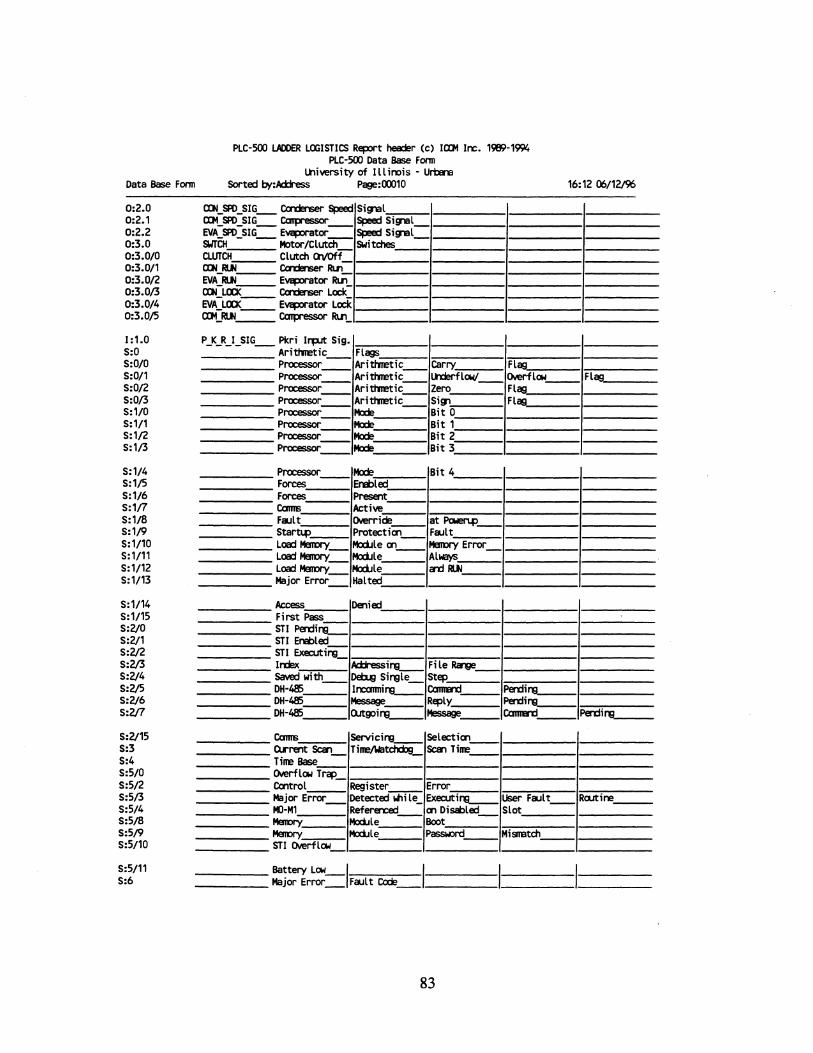
PLC-SOO LAOOER LCXiI5T1CS Rep:>rt header (c) I(DI In::. 1se9'1~ PLC-SOO Data Base Fonn

lhi vers i ty of Illi roi s - Urbana Data Base Fonn Sorted bf:Ad:lress Page:!XXl10 16: 12 06/12/%

0:2.0 0:2.1 0:2.2 0:3.0 0:3.0/0 0:3.0/1 0:3.0/2 0:3.0/3 0:3.0/4 0:3.0/5

1:1.0 5:0 5:0/0 5:0/1 5:0/2 5:0/3 5:1/0 5:1/1 5:1/2 5:1/3

5:1/4 5:1/5 5:1/6 5:1/7 5:1/8 5:1/9 5:1/10 5:1/11 5:1/12 5:1/13

5:1/14 5:1/15 5:2/0 5:2/1 5:2/2 5:2/3 5:2/4 5:2/5 5:2/6 5:2!7

5:2/15 5:3 5:4 5:5/0 5:5/2 5:5/3 5:5/4 5:5/8 5:5/9 5:5/10

5:5/11 5:6

CXlI SPO 51G cadenser Speed 5i gla l (DI:SPO)IG catpressor __ Speed ·'='5i:-gla--;""l-;�-----II-----II-----

EVA_SPO_5IG_ Evcp:!I"ator __ Speed 5iglal __ I------I------,------S\lTCH Motor/Clutch SWitches ,-CLUTCH Clutch QVOff '---1------1------1-----CXlI ~ cadenser Rul

EVA:~ E~torRul~_-:~~~~~~:::=.I------I------I-------CXlI LOCK cadenser Lock EVA:LOX Evcp:!I"atorLail-------I------I------I·-----(DI_~ ___ catpressor Rul_, _______ , _____ , ______ , _____ _

P_K_R_I_5IG_ PIeri lrp..rt: 5ig. _____ Aritl1retic __ Flags

Ari tI1retic __ carry Fl8!l _____ Processor __ _____ Processor __ _____ Processor __ _____ Processor __ _____ Processor ___

Aritl1retic __ Lrderfla.l/ __ OtIerflow __ Fl8!l

Processor ------Processor

Aritl1retic Aritl1retic Mode Mode Mode _____ Processor ___ Mode

Processor Mode ----- Forces --- Ersb led

Forces Present ------ cams Acti VI:! ______ Fault C>.<er ride __

ectiCJ'l leCJ'l-

______ 5tart~ ___ Prot

le le

_____ Load MerrDry_ McdJ _____ Load MerrDry_ McdJ _____ Load MerrDry_ McdJ _____ Major Error_ Halt ed

_____ Access Pass ______ First

_____ STI Perd _______ STI E ______ STI Ex _____ Irdex

illL-nrbled ecutil'"El

saved -----DH-485

with __

_____ DH-485 _____ DH-485

cams ------ Qrra'lt 5c:a'l_

Base _____ Tine ______ ()"erf

_____ CCJ'ltro ______ Major _____ KJ-M1

low TrCIP. l __

Error_

----MerrDry Mermry

------ STI ()"e rflow

Denied

Ad:lressi~ ~ 5il'"Elle __ Ircanni '""----Message--CUtgoil'"El __

Servicil'"El __ Tine/Watchcb!L

Register __ Detected liIi le _ Referen::ed __ McdJle McdJle

Zero Fl8!l 5igl Fl8!l Bit 0 Bit 1 Bit 2 Bit 3

Bit 4

at~ Fault MEmJry Error Always a-d~

File~ 5tEP. CcmtEn::t __ PErdil'll Reply Perdil'll Message--

CcmtEn::t __ Perdil'"El ___

SelectiCJ'l 5c:a'l T illl!

Error Executi,",,---- User Faul t __ Rrutine ___ CJ'lDisabled_ 5lot Boot PIISSIoOI"d __ MiSIIBtch

----- Battery Low_I 1 ___________ 1

_____ _

_____ Major Error_ Fault COde _________________ _

83

Data Base Form

S:7 S:8 S:9 S:10 S:11 S:12 S:13 S:14 S:15 S:16

S:17 S:18 S:19 S:2O S:21 S:22

. S:23 S:24 S:25 S:26

S:27 S:2B S:29 S:3O S:31 S:32 83:0 83/0 83/1 83/2

83/3 N7:0 N7:1 N7:2 N7:3 N7:4 N10:0 N10:1 N10:2 N10:3

PLC-SOO LADDER LOOISTICS Report I1eeder (e) ICDI Ire. 1989-1994 PLC-SOO Data Base Form

lhiversity of III irois - Urt:ma Sorted b(:Address Page:1XX)11

----~------~--_____ Actiw Nodes

Act i w Nodes ----- 110 Slot

I/O Slot-­----- Math Register _____ Math Register

Node Address/ -----~ Sirele -

Ccx:Ie File

Ersbles Ersbles

Bad Rate Step Ru1l

_____ ~ Sirele_ Step _____ ~ Sirele_ SteP. _____ ~ Sirele_ SteP.

File

--~ Faul t/ Powen:brI -----~ Fault/- Powen:brI _____ Maxinun--= c:b;erve:I --

--Average San ----- Irdex --- Regi

Tine ster

_____ I/O Intern.pt Pen:! _____ I/O Intern.pt Pen:!

illl illl

I/O Intern.pt_ Ersbled I/O Intern.pt_ Ersbled User Fault Routine ___ STI 5etpoi~ STI File __ Nurtler I/O Intern.pt_ Executilll

PRS RI FAL CtwG_LIM -CLU_CYC_ENA_

Pressu-e Risire or Fallilll __ 01a-ged Limits_ Ersble Clutch_ Cycl illl

Sf'D_CHNG __ Motor Speeq_ 01a-ged Flag HI PRESS Clutch O'l Pressu-e LO-PRESS-- Clutch Of-f-- Pressu-e EVA_Sf'D_REQ Evaporator Speed Req..est WLSf'D_REQ_ Ccrdenser Speed Req..est CDI_ Sf'D _ REQ_ Ccrrpressor __ Speed Req..est CAL SLCP TrlYlSd..l;:er cal ib. Slc:pe CAL=OFF - TrlYlSd..l;:er cal ib. Offset P CDN TMP 1 Press. Ccrr.Irs. T81p. Var. 1 P=(Dj(TMP) Press. Ccriv.-= T81p. Var. 2

P_CDN_TMP_3_ Press. Ccriv._ T81p. Var. 3 HI PRESS INT Hig, Press. Integer LO-PRESS-INT- Low Press. - Int~ EVA_Sf'DjW - Evaporator Speed Top. Var . (Dj_Sf'D_TMP_ Ccrdenser Speed Top. Var. CDI_Sf'D_TMP_ Ccrrpressor __ Speed Top. Var.

Main Caltr ol Progran

8reakplint __ 8reakplint __ Ru1l File San Tine

Fi le Nurtler

Irdicator

(x 100) (x 10000)

----- Main Clute h Cycl ire __ Progran

Ru1l File

re Limits

16: 12 06/12/%

N10:4 N10:5 N10:6 N10:7 N10:8 N10:9 PFILE:002 PFILE:003 PFILE:004 PFILE:005

Ca"r.ierts C lutch Cycl ----- Ca"r.ierts M otor Speeq

ire Pressu __ s

U:3 U:4

CCR Clutch Cycl ire_I Rout i ne ___ 1 1 11 ____ _

LCR:---- Clutch Cyclire_ Pressure Limit_ Co'1Versicn __ Routine ___ I _____ _

84

Appendix D. Charge Optimization Test Plans This Appendix contains the test plans we used to determine the optimum charge for

refrigerant system operations. These tables are included as background for the plots

presented in Section 3.2, Charge Optimization.

We reiterate here that the term "optimum charge" used in the context of this thesis

refers to a particular vehicle manufacturer's test specification for initial charging of air

conditioning system. "Optimum" in this context is not used as one might expect, that is,

charge is not adjusted to maximize or minimize any particular performance measure of the

system. In the test specification, "optimum charge" is defined as that charge for which the

refrigerant temperatures at the inlet and outlet of the evaporator first "cross over." That is,

the optimum charge is the charge for which it is observed that the refrigerant exiting the

evaporator is not superheated.

85

Table 0.1 Single Point Charge Optimization Test Plan

Charge Optimization Test Plan: I-point optimization Project 51 Mobile Air Conditioning Systems

Objective: Determine optimum refrigerant charge for system installed in lab

DefInitions: optimum charge: that charge at which evaporator refrigerant

inlet and outlet temps fIrst cross over.

Test Stand Conditions:

Condenser Air Flow: Condenser Inlet Air Temp: Evaporator Air Flow: Evaporator Inlet Air Temp: Compressor Speed:

Method:

1800cfin 110 deg F 300cfin 110 deg F 1200 rpm

1) Charge loop to initial refrigerant mass of 2.5 Ibs 2) Establish steady-state conditions 3) Log data 4) If evap ref in = evap ref out then OPTIMUM charge obtained - test complete 5) If evap ref in < evap ref out -- add .05 Ib charge 6) Repeat - starting at step 2

I Charge Level Steady IData Logged File [lbs] 2.50 2.55 2.60 2.65 2.70 2.75 2.80 2.85 2.90 2.95 3.00 3.05 3.10 3.15 3.20

86

Table D.2 Varying Parameters Charge Optimization Test Plan

Charge Optimization wI Varying Parameters Test Plan Project 51 Mobile Air Conditioning Systems

Objective: obtain steady-state and transient performance data for a range of test conditions and refrigerant charge levels in the neighborhood of the optimum charge test conditions and the optimum charge .

Test Parameters

Charge (w/r/t optimum) : Condenser Inlet Air Temp: Evaporator Inlet Air Temp: Condenser Air Flow: Evaporator Air Flow: Compressor Speed:

typical Test Matrix

I Charge

Teat Teal 11U 110 110 110 120 IOU 120 100 110 IOU 110 100 IOU IOU 100 100 110 90 110 90 110 110 110 110

12 tests per charge level 5 charge levels 60 tests total

0.85, 0.90, 0.95, 1.00, 1.05, 1.10 100, 110, 120

90, 100, 110 1800cfm 300cfm 1200 rpm, 3000 rpm

Ncomp Steaay 1200 x 3600 x 1200 x 3600 x 1200 x 3600 x 1200 x 3600 x 1200 x 3600 x 1200 3600

87

-CycIOOClutcn

x x

Appendix E. Experimental Facility Energy Balance Validation The following discussion concerns outstanding issues which relate to obtaining

satisfactory agreement between air side and refrigerant side heat transfer measurements for

each heat exchanger. Specifically, the Validity of some conclusions in [2] regarding the

condenser energy balance are brought into question.

This issue does not bring into question the integrity of the results of the refrigerant

charge loss experiments reported in Chapter 4 of this thesis, which focused exclusively on

refrigerant side temperature and pressure measurements. The refrigerant side

instrumentation is accurate. Strong proof of this statement is provided by Figure 4.5.

During each off cycle of the compressor, the refrigerant state at the evaporator outlet

becomes saturated. In Figure 4.5, notice the excellent agreement we obtained between the

refrigerant temperature measured by immersion thermocouple and the saturation

temperature calculated from the measured refrigerant pressure.

In Figure E.t, we present the results of steady state tests conducted specifically to

check the agreement of the heat transfer rates measured on the air side and the refrigerant

side of the heat exchangers, and to verify the energy balance agreement claimed by in [2].

The data were collected over a wide range of air flow rates, compressor speeds, and air

temperatures. The evaporator data plotted in Figure E.t show that the evaporator energy

balance is satisfactory, and generally demonstrate agreement with the claim in [2] to have

obtained 5% agreement over 68% of the data. The condenser data clearly demonstrate that

there is a systematic bias which causes the measured refrigerant side heat transfer rate to

exceed the measured air side heat transfer rate by about t 0%. Table E.t reports the mean

error and absolute average error, with associated standard deviations, for the evaporator

and condenser energy balances.

20

5

Evaporator Enel'lY Balance

o eabI [dol BIuIhr]

_+I.,'" ......... +I. lOll

O ............................................................................... ____ .......... ..J....... .......... ........J

o 5 10 15 20 25

erblJDicro [xlU BtuIbr]

25

20

i 15 III

~ .!!. ii 10 u

5

0 0

Coadeaser Eael'lY Balaace

/ .. ' o call! [dO' 1IIuIbr] / ~ •• "" .•• ;' _+/.,... / ..... . ,'6o.P

......... +I. lOll / :-:: ••.• :;...-jf( / ........ Q.6Y

5

/~~'/d~ ~ ••• --. 0'· 0

/..' 0 ~.::~ 0

Lf.:.;·/ ;(. •••• ;;. 00

,(,.,::.,;; .;,; .... 0

10 15

crbCmicro [xlO' Blulbr]

20 25

Figure E.t Steady-State Energy Balances: Evaporator and Condenser

88

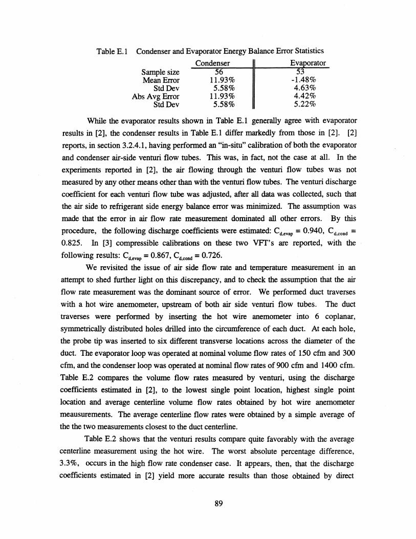
Table E.I Condenser and Evaporator Energy Balance Error Statistics

Sample size Mean Error

StdDev Abs Avg Error

StdDev

Condenser 56

11.93% 5.58%

11.93% 5.58%

Eva orator 53

-1.48% 4.63% 4.42% 5.22%

While the evaporator results shown in Table E.l generally agree with evaporator

results in [2], the condenser results in Table E.l differ markedly from those in [2]. [2]

reports, in section 3.2.4.1, having performed an "in-situ" calibration of both the evaporator

and condenser air-side venturi flow tubes. This was, in fact, not the case at all. In the

experiments reported in [2], the air flowing through the venturi flow tubes was not

measured by any other means other than with the venturi flow tubes. The venturi discharge

coefficient for each venturi flow tube was adjusted, after all data was collected, such that

the air side to refrigerant side energy balance error was minimized. The assumption was

made that the error in air flow rate measurement dominated all other errors. By this

procedure, the following discharge coefficients were estimated: Cd,evap = 0.940, Cd,CODd = 0.825. In [3] compressible calibrations on these two VFT's are reported, with the

following results: Cd,evap = 0.867, Cd,CODd = 0.726.

We revisited the issue of air side flow rate and temperature measurement in an

attempt to shed further light on this discrepancy, and to check the assumption that the air

flow rate measurement was the dominant source of error. We performed duct traverses

with a hot wire anemometer, upstream of both air side venturi flow tubes. The duct

traverses were performed by inserting the hot wire anemometer into 6 coplanar,

symmetrically distributed holes drilled into the circumference of each duct. At each hole,

the probe tip was inserted to six different transverse locations across the diameter of the

duct. The evaporator loop was operated at nominal volume flow rates of 150 cfm and 300

cfm, and the condenser loop was operated at nominal flow rates of 900 cfm and 1400 cfm.

Table E.2 compares the volume flow rates measured by venturi, using the discharge

coefficients estimated in [2], to the lowest single point location, highest single point

location and average centerline volume flow rates obtained by hot wire anemometer

meausurements. The average centerline flow rates were obtained by a simple average of

the the two measurements closest to the duct centerline.

Table E.2 shows that the venturi results compare quite favorably with the average

centerline measurement using the hot wire. The worst absolute percentage difference,

3.3%, occurs in the high flow rate condenser case. It appears, then, that the discharge

coefficients estimated in [2] yield more accurate results than those obtained by direct

89

Table E.2 Comparison of Air Volume Flow Rate Measurement: Venturi vs. Hot Wire Anemometer

Condenser Eva orator Nominal [cfm] 1400 900 300 Venturi [cfm] 1420 885 316

Hot Wire Anemometer Maximum [cfm] 1480 920 330

Average Centerline [cfm] 1375 880 300 Minimum [cfm] 1190 740 276

150 149

156 148 142

Non-uniformity 21.0% 20.5% 18.0% 9.5%

calibration in [3]. Let us now define the tenn non-uniformity as the ratio of the difference

between the minimum and maximum flow rate to the average centerline flow rate. By this

rough measure it appears that non-uniformity is significant in three out of four cases.

Accurate venturi flow tube measurements require unifonn inlet flow profiles. In the

absence of a direct calibration with air, as discussed in [3], it is not clear what effect the

non-uniformity has on the venturi performance. It is true that the convergent at the inlet to

the venturi flow tube will tend to mitigate the severity of the non-uniformity. The data in

Table E.2 imply that the discharge coefficients from [2] may be used, but only in concert

with conservative uncertainties.

Figure E.2 plots airside and refrigerant side heat transfer rates, calculated from

experimental data obtained in the first charge optimization experiment, versus refrigerant

charge. This plot is not directly related to detennining optimum charge, rather it clearly

illustrates some characteristics of our test facility design and data reduction that bear

explanation. The fIrst point clearly illustrated by Figure E.2 is that, in general, the

agreement between air side and refrigerant side heat transfer rate calculations is significantly

better for the evaporator than for the condenser. We notice that, in all cases, the condenser

air side heat transfer, caht, is significantly less than condenser refrigerant side heat

transfer, crht and crhCmicro.. Figure E.2 also illustrates the close agreement between

refrigerant side heat transfer rates calculated using mass flow rates obtained from liquid

venturi measurements, erht and crht, and from coriolis meter mass flow rate measurements,

erhCmicro and crhcmicro. This supports the Validity of the liquid venturi calibration and

mass flow rate calculation. Figure E.3 presents the same information as Figure E.2,

however the energy balance discrepancy is presented as a percentage of the refrigerant side

heat transfer rate.

90

25

~ 20 ~ -~ ..., 0 -...... 15 ! ... ~ '" § = 10 -a ~ .c

5

o 0.0

Airside and Refrigerant Side Heat Transfer

I). caht [Btulhr] ¢ crht [BtuIhr]

8~ 0 crhunicro [BtuIhr] 0 eaht [BtuIhr]

t.t.~ 0 erht [BtuIhr] + erhunicro [BtuIhr] Q~

caht = cond air heat transfer crht = cond ref heat transfer, liquid venturi mass flow rate crhcmicro = cond ref heat transfer, Micromotion mass flow rate

eaht = evap air heat transfer erht = evap ref heat transfer, liquid venturi mass flow rate erhcmicro = evap ref heat transfer, Micromotion mass flow rate

1.0 2.0 Charge [lbs]

3.0 4.0

Figure E.2 Charge optimization: Heat transfer rates versus refrigerant charge level.

20

10

~

I .~

~~ 0

-10

-20 0.0

Energy Balance Error

t. cEbal [%] I).

0 cEbal_micro [%] lID 1).$ ¢ eEbal [%] D~ 0 eEbal_micro [%] I).

0

¢

o~ ¢<i:9

~~

cEbal = cond energy balance error, liquid venturi mass flow rate cEbal_micro = cond energy balance error, Micromotion mass flow rate

eEbal = evap energy balance error, liquid venturi mass flow rate eEbal_micro = evap energy balance error, Micromotion mass flow rate

1.0 2.0

Charge [lbs]

3.0

Figure E.3 Energy balance errors as a function of refrigerant charge.

91

4.0

The evaporator energy balance agreement deteriorates at higher charges because the

refrigerant at the evaporator outlet approaches saturation, and then becomes two-phase.

We assume superheated conditions at the outlet of the evaporator in order to obtain a

refrigerant enthalpy from temperature and pressure measurements. At higher charges this

assumption is violated, the refrigerant enthalpy is overestimated, and the redundant check

on the air side instrumentation is lost.

There is a slightly different reason why the condenser air side and refrigerant side

heat transfer measurements depart by a greater degree at higher charge levels than at low

charge levels. We know that subcooling actually becomes greater as more charge is added,

and we said that air side and refrigerant side heat transfer calculations compare more

favorably when the outlet refrigerant is single phase, so we would expect that the

agreement would improve as charge is added. However, the air side temperature

measurement at the outlet of the condenser is very likely subject to a large, systematic error.

In Section 3 we described the test facility and explained that air temperatures are measured

using grids of thermocouples wired in parallel, which spatially averages the temperature

profile being measured. The grid spacing and mixing arrangement currently used in the

condenser loop is probably insufficient to measure the actual spatial average temperature.

In fact, it is likely that this temperature is being underestimated in many cases. As the

amount of charge in the system increases, the amount of two-phase and subcooled

refrigerant in the condenser increases, which causes a highly non-uniform temperature

profile at the outlet.

We note here that the issues concerning condenser energy balances, in particular, is

an ongoing problem that will affect the experimental estimation of two-phase refrigerant

properties at the condenser and evaporator outlets, and merits further investigation and

correction. As stated earlier in this Appendix, these issues are separate from, and do not

affect, the integrity of the refrigerant side temperature and pressure measurements.

Figure EA is presented to further illustrate the nature of the issue of air side heat

transfer measurement. Figure EA plots the differential temperature and the volume flow

rate of the air stream across each heat exchanger. We immediately note that the condenser

air stream has a higher volume flow rate and lower differential temperature than the

evaporator. In fact, the typical air side differential temperature across the condenser is

10 F to 12 F, while the typical differential temperature across the evaporator is about

50 F. We clearly see that a bias, or systematic error, of, say, 1 F, in the temperature

measurement across the condenser will cause a much greater error in the heat transfer rate

calculation (approx. 10%) than will a bias of equal magnitude in the evaporator temperature

measurement (approx 2%). In other words, the fractional contribution of the temperature

92

80.0

60.0

[i;

:K 40.0 E-< <I

20.0

0.0

0.0

Airside Heat Transfer

o dTcond [deg F] o dTevap [deg F]

• Qcav [cfm] e Qeav [cfm]

dTcond = cond air differential temp dTevap = evap air differential temp Qcav = volume flow rate, cond air venturi Qeav = volume flow rate, evap air venturi

1.0 2.0 Charge [lbs]

elllllllli o QOOOOOOOO

3.0

2000

1500

1000

500

o 4.0

Figure E.4 Air side heat transfer rate as a function of refrigerant charge.

< 0

=-3 n ::l 0 ~

a n n l

measurement to an error in the heat transfer calculation is much greater for the condenser

than for the evaporator.

93

Appendix F. Clutch Cycling Data Table F.l Clutch Cycling Data

Experiment Run # Cycles AvgPeriod AvgOffTime 1 1 27 22.9 11.0

2 26 24.3 10.3 3 28 22.0 9.0 4 24 25.8 10.0 5 24 26.3 8.7 6 30 20.1 7.8 7 19 31.4 10.0 8 18 32.2 8.7 9 18 33.1 12.0 10 19 32.1 10.0 11 10 55.3 13.5 12 12 47.4 12.7 13 14 43.6 11.0 14 23 26.3 8.7 15 16

2 1 22 28.0 13.0 2 25 24.2 11.5 3 25 24.4 9.0 4 30 21.1 9.8 5 25 24.8 9.3 6 27 23.0 8.5 7 20 29.9 6.3 8 17 32.8 7.7 9 20 31.2 12.3 10 15 39.4 16.5 11 17 34.6 11.5 12 17 36.1 13.3 13 20 30.4 12.5 14 20 29.9 9.3

3 15 9 61.4 nla 3 16 6 57.7 nla

94

Run 2-1

10 __ Pero

......... Tero __ scaled RPM

o ~~~~~~~~~~~~~~~~ 300 320 340 360 380 400

time[seel

Evaporator Ref ........ t Outlet

50

K!4O I! I 30 ! .. 220

10 --Pero .......... Tao --oc:aledRPM

0 300 320 340 360 380 400

time [,..,1

Evaporator RefrI .... aat Outlet 60

Run 2-3

50

K~4O I!

h 30

H2O 10

__ Pero

~ .......... Tao --scaled RPM

0 300 320 340 360 380 400

time[seel

E"porator RefrI ...... t Outlet 60

Run 2-4

50

K~4O I 30 !J 20

10 __ Pero

····.···Tero __ scaled RPM

0 300 320 340 360 380 400

Iime[seel

Evaponlor Rorripnnt Oullet

Run 2-9

10 --Pero ····.···Tero --scaled RPM

o 300 320 340 360 380

Iime[seel

E •• po ... tar Relriprant Outlet

Run 2-10

10

__ Pero

·•·· ... ···Tero --scaled RPM

o~~--.. ~~~~~~--~~~--~ 300 320 340 360 380 400

time[seel

Evaponlor Refripraal OatIet

Run2-11

10 --Poro •·· ... ···Tero --scaled RPM

O~~~~~~~--~~----~~~~

400

300 320 340 360 380 400 time[secl

Evaporatnr RefrI ....... t Oudet

Run 2-12

....• -.. Tero --scaled RPM o ~~~~~~~~--~~~~~~~~

300 320 340 360 380 400 Iime[seel

Figure F.l Experiment 2: Evaporator outlet refrigerant temperature and pressure time histories [Runs 2-1 through 2-4; Runs 2-9 through 2-12]

95

Evaporator Refriprant Outlet 00 ~ __ ~~~~~~~ ____ ~ __ ~~

so

i140

~ 30

H2O 10

···· .. ···Tao --scaled RPM OL... ................ L....o. ........ ......JI........ ................ ____ ......................... .....:J

300 320 340 300 380 400

so

i~4O 1~3O ~i 20

10

lime (sec]

_Pero ~··· .. ···Tero --scaled RPM oJ:...... ........ ......JI........ ................. __ ................................. _ ....... ....J

300 320 340 300 380 400 lime (sec]

E.apondor RefrlgeraDI OUllel

00 ~----r-----r-----r-~--r-~~ Run 2-7

10 __ Pero

......... Tao --scaled RPM ol:-o--... ................. --... .................................................................... .........:J

300 320 340 300 380 400 lime (sec]

E.aporator Refrileraul Ouliel

RUD2-8

10 --Pero ···· .. ···Tao --scoledRPM o J:...... ........ ......JI........ ................ __ ......................... ~ ........ ~~

300 320 340 300 310 400 lime (sec]

Run 2-13

so

i140

M 30

H20

10

__ Pero

•·· ..... ··Tero --scaled RPM Ot..... ....... __ ...1-............ -L. ........ __ ...... -'-............. I0...." ...... -..l

300 320 340 300 380 400 Iime(...,]

E ...... rater Refriprul OUliet

Run 2-14

so

10

oJ:...... ................ L....o. ........ ......JL....o. ................ I........ ................ ___ ........ ~

300 320 340 300 380 400 time(...,]

Evaporator RefrileraDI Oudel oo ....... --....-I"""""'--"P-J---O"""T--....... '"""T"--..-."""]

so

li 40

~ 30 Ie d20

10

RUD3-15

_Perc .~ .... ~ .. Tao __ scaled RPM

oJ:...... ................ L....o. ................ __ ......................................... ~....J

300 320 340 300 380 400 time("",]

E._rater Refriaerant Ollllel

Rua3-16

so

10 __ Pero

........ - Tero __ scaled RPM

340 380 420 460 500 time (sec]

Figure F.2 Experiment 2: Evaporator outlet refrigerant temperature and pressure time histories [Runs 2-5 through 2-8; Runs 2-13, 2-14, 3-15, 3-16]

96