Experimental study of image representation spaces in variational disparity calculation

Ralli et al. EURASIP Journal on Advances in Signal Processing 2012, 2012:254http://asp.eurasipjournals.com/content/2012/1/254

RESEARCH Open Access

Experimental study of image representationspaces in variational disparity calculationJarno Ralli*, Javier Dıaz, Pablo Guzman and Eduardo Ros

Abstract

Correspondence techniques start from the assumption, based on the Lambertian reflection model, that the apparentbrightness of a surface is independent of the observer’s angle of view. From this, a grey value constancy assumption isderived, which states that a change in brightness of a particular image pixel is proportional to a change in its position.This constancy assumption can be extended directly for vector valued images, such as RGB. It is clear that the greyvalue constancy assumption does not hold for surfaces with a non-Lambertian behaviour and, therefore, theunderlying image representation is crucial when using real image sequences under varying lighting conditions andnoise from the imaging device. In order for the correspondence methods to produce good, temporally coherentresults, properties such as robustness to noise, illumination invariance, and stability with respect to small geometricaldeformations are all desired properties of the representation. In this article, we study how different imagerepresentation spaces complement each other and how the chosen representations benefit from the combination interms of both robustness and accuracy. The model used for establishing the correspondences, based on the calculusof variations, is itself considered robust. However, we show that considerable improvements are possible, especially inthe case of real image sequences, by using an appropriate image representation. We also show how optimum (ornear optimum) parameters, related to each representation space, can be efficiently found.

IntroductionThe optical flow constraint [1], based on the Lambertianreflection model, states that a change in the brightnessof a pixel is proportional to a change in its position, i.e.,the grey level of a pixel is assumed to stay constant tem-porally. This same constancy concept can be used also indisparity calculation by taking into account the epipolargeometry of the imaging devices (e.g., a stereo-rig). Thegrey level constancy, that does not hold for surfaces witha non-Lambertian behaviour, can be extended for vec-tor valued images with different image representations.In this study, we use a method based on the calculusof variations for approximating the disparity map. Vari-ational correspondence models typically have two terms,the first one being a data term (e.g., based on the grey levelconstancy), while the second one is a regularisation termused to make the solution smooth. In order to make thedata term more robust with respect to non-Lambertian

*Correspondence: [email protected] de Arquitectura y Tecnologıa de Computadores, EscuelaTecnica Superior de Ingenierıas y de Telecomunicacion, Universidad deGranada, Calle Periodista Daniel Saucedo Aranda s/n, E-18071 Granada, Spain

behaviour, different image representations can be used.Some of the problems in establishing correspondencesarise from the imaging devices (e.g., camera/lens parame-ters being slightly different, noise due to imaging devices)and some, from the actual scene being observed (e.g.,lighting conditions, geometrical deformations due to cam-era setup). Typically, illumination difference and opticsrelated ‘errors’ are modelled as a multiplicative type oferror, while the imaging device itself is modelled as a com-bination of both multiplicative and additive ‘errors’. It isclear that the underlying image representation is crucial inorder for any correspondence method to generate correct,temporally coherent estimates in ‘real’ image sequences.In this article, we study how combinations of differ-

ent image representations behave with respect to bothillumination errors and noise, ranking the results accord-ingly. We believe that such information is useful to thepart of the visual community that concentrates on appli-cations, such as obstacle detection in vehicle related sce-narios [2], segmentation [3], and so on. Although otherauthors address similar issues [4,5], we find these to beslightly limited in scope due to a reduced ‘test bench’,

© 2012 Ralli et al; licensee Springer. This is an Open Access article distributed under the terms of the Creative CommonsAttribution License (http://creativecommons.org/licenses/by/2.0), which permits unrestricted use, distribution, and reproductionin any medium, provided the original work is properly cited.

Ralli et al. EURASIP Journal on Advances in Signal Processing 2012, 2012:254 of 19http://asp.eurasipjournals.com/content/2012/1/254

e.g., a small number of test images or image representa-tions. Also, in most of the cases, the way in which theparameters related to the model(s) have been chosen isnot satisfactorily explained. Therefore, the main contri-bution of our article is an analysis of the different imagerepresentations supported by a more detailed and sys-tematical evaluation methodology. For example, we showhow optimum (or near optimum) parameters for the algo-rithm, related to each representation space, can be found.This is a small but important contribution in the case ofreal, non controlled, scenarios. The standard image rep-resentation is the RGB-space, the others being (obtainedvia image transformations): gradient, gradient magnitude,log-derivative, HSV, rφθ , and phase component of animage filtered using a bank of Gabor filters.This work is a comparative study of the chosen image

representations, and it is beyond the scope of this arti-cle to explain why certain representations perform betterthan others in certain situations. Under realistic illumi-nation conditions, with surfaces both complying and notcomplying with the Lambertian reflection model, theoret-ical studies can become overly complex, as we show next.It is typically thought that chromaticity spaces are illumi-nation invariant, but under realistic lightning conditions,this is not necessarily so [6]. One of the physical modelsthat explains light reflected by an object is the Dichro-matic ReflectionModel [7] (DRM), which in its basic formassumes that there is a single source of light [7], whichis unrealistic in the case of real images (unless the light-ning conditions can be controlled). A good example of thisis given by Maxwell et al. in their Bi-Illuminant Dichro-matic Reflection article [6]: in a typical outdoor case, themain illuminants are sunlight and skylight, where fullylit objects are dominated by sunlight while objects in theshade are dominated by skylight. Thus, as the illumina-tion intensity decreases, the hue of the observed colourbecomes bluish. For the above mentioned reasons, chro-matic spaces (e.g., HSV, rφθ ) are not totally illuminationinvariant under realistic lightning conditions. Therefore,in general, we do not speak of illumination invariancein this article but of illumination robustness or robustimage representation with respect to illumination changesand noise. By illumination error, we refer to varying illu-mination conditions between the left- and right stereocameras.Next, Section 1 presents the relevant related study, some

sources of error, and the variational method. Finally, inSections 1, 1, and 1, we describe the proposed methodolo-gies, results, and conclusions.

Backgroundmaterial and related studyRelated studyThe idea of robust ‘key-point’ identification is an impor-tant aspect of many vision related problems and has

lead to such concepts as SIFT [8] (scale invariant fea-ture transform) or SURF [9] (speeded up robust features).This study relates to identifying robust features as well,however, in the framework of variational stereo. Severalstudies comparing different data- or smoothness termsfor optical-flow exist, for example, those of Bruhn [10]and Brox [11]. A similar study to the one presented here,carried out in a smaller scale for the optical-flow, hasbeen done by Mileva et al. [4]. On the other hand, in[5], Wohler et al. describe a method for 3D reconstruc-tion of surfaces with non-Lambertian properties. How-ever, many comparative studies do not typically explainin detail how the parameters for each different competingalgorithm or representation were obtained. Also, some-times it is not mentioned, if the learn and test sets forobtaining the parameters were the same. This poses prob-lems related to biasing and over-training. If the param-eters have been obtained manually, they are prone tobias from the user: expected results might get confirmed.On the other hand, if the learn and test sets were thesame or they were too small, it is possible that over-training has taken place and, therefore, the results arenot generalisable. We argue that in order to properlyrank a set of representation spaces or different algo-rithms, with respect to any performance measure, opti-mum parameters related to each case need to be searchedconsistently, with minimum human interference, avoidingover-fitting.Where our study differs from the rest is that (a) we use

an advanced optimisation scheme to automatically opti-mise the parameters related to each image representationspace, (b) image sets for optimisation (learning) and test-ing are different in order to avoid over-fitting, (c) we studythe robustness of each representation space with respectto several image noise and illumination error models, and(d) we combine the results for both noise and illumina-tion errors. Thus, the methodology can be considered tobe novel.

Sources of errorSince the approach of this article is more experimen-tal than theoretical, we only quickly cover some of thesources of error suffered by correspondence methods.Although optical-flow and stereo are similar in nature,they differ in a very important aspect: in stereo, theapparent movement is due to a change of position ofthe observer (e.g., left and right cameras), whereas in theoptical-flow case, both the observer and the objects inthe scene can move with respect to each other. Thus,stereo and optical-flow do not suffer from exactly the sameshortcomings. For example, in the case of stereo, shad-ows cast upon objects due to illumination conditions canprovide information when searching corresponding pixelsbetween images. In the case of optical-flow, a stationary


shadow cast upon a moving object makes it more difficultto find the corresponding pixels. Also, as it was alreadymentioned in Section 1, the imaging devices also causeproblems in the form of noise, motion blur, and so on.Thus, an image representation space should be robustwith respect to (a) small geometrical deformations (geo-metrical robustness), (b) changes in the illumination level(illumination robustness), both global and local, and (c)noise present in the images (e.g., due to the acquisitiondevice). Our analysis was carried out for stereo but isdirectly applicable to optical-flow as well.

Variational stereoWe have chosen to use a variational method for severaldifferent reasons: (a) transparent modelling of the corre-spondence problem; (b) extending the model is straight-forward; (c) the samemathematical formalism can be usedfor both optical-flow and stereo; and (d) the governingdifferential equation(s) can be solved efficiently [12]. Theoriginal idea of solving optical-flow in a variational frame-work is by Horn and Schunck [1]. The particular methodthat we have used was introduced by Slesareva et al. in[13] and is based on the optical-flow method of Broxet al. [14]. The characteristics of this method are: errorfunctions for both the data and the regularisation termsare non-quadratic [14,15]; the regularisation term is non-linear isotropic [12,16], based on the flow (flow-driven)and warping over several scales (multi-resolution strat-egy) is used in order to recover greater displacementswith late linearisation [14,17,18] of the constancy terms.A Matlab/MEX code of the algorithm can be downloadedfroma.Before going any further, we introduce the used nota-

tion, so that the rest of the text would be more readable.

NotationWe consider the (discrete) image to be a mapping I(�x, k) :� → R

K+, where the domain of the image is � :=[ 1, . . . , N]×[ 1, . . . , M], M and N being the numberof columns and rows of the image, K defines numberof the channels, and �x = (x, y). In our case K =3, since the input images are RGB, that is, I(�x, k) :=[R(�x) G(�x) B(�x)]. The input image is then transformedinto the desired image representation by I(�x, k) →T(�x, kt) so that T(�x, kt) : � → R

KT+, where KT is thenumber of channels of the transformed image and � is asdefined previously. We use subindices L and R to refer tothe left- and the right images. Superindex w means thatthe components in question are ‘warped’ using the dis-parity d. For example, Tw

R = T(x + d(x, y), t

)R means

that all the components of the right image are warped asper disparity d = d(x, y). For ‘warping’ we use bilinearinterpolation.

ModelThe energy functional to be minimised is as follows:

E(d) =∫

�

( 2∑t=1

btDt(TL,TR, d)

)dx + α

∫�

S(∇d)dx

E(d) =∫

�

⎛⎝b1D1(TL,TR, d) + b2D2(TL,TR, d)︸︷︷︸

combined data term

⎞⎠dx

+ α

∫�

S(∇d)dx(1)

whereD1(IL, IR, d) andD2(IL, IR, d) are components of thecombined data term, S(∇d) is the regularisation term, andT{L,R} refers to the transformed versions of the left and theright images (all the channels). b1 ≥ 0, b2 ≥ 0 and α ≥ 0are the parameters of the model, defining the weight of thecorresponding term. Both the data and the regularisationterms are defined as:

Dt(TL,TR, d) :=KT∑kt=1

�(∥∥TL,kt − Tw

R,kt∥∥22

), ∀t

S(∇d) := �(‖∇d‖22

) (2)

where TL,kt = T(x, y, kt

)L is the ktth channel of the left

transformed image,TwR,kt = T

(x+d(x, y), y, kt

)R is the ktth

channel of the right transformed image warped as per dis-parity d = d(x, y), �(s2) = √

s2 + ε2 is a non-quadraticerror function, and ‖ · ‖2 is the L2 norm. For ‘warping’we use bilinear interpolation. We would like to point outthat even if formal definitions for all the Dt are ‘equal’,the used image representation (i.e., transformation) is notnecessarily the same for each t. We could have used anadditional index for pointing out this fact, but we feel itshould be clear from the context.Because of the ambiguities related to the different rep-

resentations and the L2 norm, here we give a concreteexample of (2) for the ∇I (see 1) and |∇I| (see 1) repre-sentations. More specifically, we use∇I representation forD1 and |∇I| for D2. For clarity’s sake, we refer directly tothe channels R, G and B, while subindices {L, R} indicatewhich image (left or right) is in question. Terms of the ∇Irepresentation are:

∇IL :=[

∂RL∂x

∂RL∂y

∂GL∂x

∂GL∂y

∂BL∂x

∂BL∂y

]

∇IR :=[

∂RR∂x

∂RR∂y

∂GR∂x

∂GR∂y

∂BR∂x

∂BR∂y

],

(3)


whereas terms of the |∇I| representation are:

|∇IL| :=[ [

∂RL∂x

∂RL∂y

] [∂GL∂x

∂GL∂y

] [∂BL∂x

∂BL∂y

]]

|∇IR| :=[ [

∂RR∂x

∂RR∂y

] [∂GR∂x

∂GR∂y

] [∂BR∂x

∂BR∂y

]](4)

In the (4) case the inner brackets (i.e., [ ·]) are used toindicate over which terms the norm is calculated. In otherwords, in (3) KT = 6, whereas in (4) KT = 3. Next step isto ‘plug’ terms of each representation into Equation (2) inorder to get the actual data terms. For the ∇I we have:

D1(∇IL,∇IR, d) = �

((∂RL∂x

− ∂RwR

∂x

)2)+ �

((∂RL∂y

− ∂RwR

∂y

)2)

+ �

((∂GL∂x

− ∂GwR

∂x

)2)+ �

((∂GL∂y

− ∂GwR

∂y

)2)

+ �

((∂BL∂x

− ∂BwR

∂x

)2)+ �

((∂BL∂y

− ∂BwR

∂y

)2)

(5)

The same for the |∇I| is:

D2(|∇IL|, |∇IR|, d) = �

((∂RL∂x

− ∂RwR

∂x

)2+(

∂RL∂y

− ∂RwR

∂y

)2)

+ �

((∂GL∂x

− ∂GwR

∂x

)2+(

∂GL∂y

− ∂GwR

∂y

)2)

+ �

((∂BL∂x

− ∂BwR

∂x

)2+(

∂BL∂y

− ∂BwR

∂y

)2)

(6)

where the superindex w refers to warping as previously,i.e., Tw

R,kt = T(x + d(x, y), y, kt

)R. In order to complete the

example, using the above mentioned representations, thecomplete energy functional would be written as:

E(d) =∫

�

(b1�

((∂RL∂x

− ∂RwR

∂x

)2)+ b1�

((∂RL∂y

− ∂RwR

∂y

)2)

+ b1�((

∂GL∂x

− ∂GwR

∂x

)2)+ b1�

((∂GL∂y

− ∂GwR

∂y

)2)

+ b1�((

∂BL∂x

− ∂BwR

∂x

)2)+ b1�

((∂BL∂y

− ∂BwR

∂y

)2)

+ b2�((

∂RL∂x

− ∂RwR

∂x

)2+(

∂RL∂y

− ∂RwR

∂y

)2)

+ b2�((

∂GL∂x

− ∂GwR

∂x

)2+(

∂GL∂y

− ∂GwR

∂y

)2)

+ b2�((

∂BL∂x

− ∂BwR

∂x

)2+(

∂BL∂y

− ∂BwR

∂y

)2))dx

+ α

∫�

�(‖∇d‖22

)dx(7)

As we can see from Equations (5) and (6), error func-tion �(·) acts differently for ‘scalar’ and ‘vector’ fields.In (5), each of the components has its own error func-tion, while in (6), the components are ‘wrapped’ inside thesame error function. In order to have a better insight howthis affects robustness, let us suppose that at a given posi-tion, the vertical derivative could not approximated welland, thus, would be considered an outlier. In the ∇I case,only the vertical derivative would be suppressed (i.e., thecomponent considered an outlier), while the horizontalderivative would still be used for approximating the dis-parity. In the |∇I| case, however, the whole term wouldbe suppressed and the horizontal derivative would not beused either for approximating the disparity.Now, with both the energy functional and the related

data terms described, a physical interpretation of themodel can be derived: we are looking for a transformationdescribed by d that transforms the right image represen-tation into the left image representation, with the d beingpiecewise smooth. By transforming the right image intothe left image, we mean that the image features describedby the data term(s) align.Since the model is well known, we only quickly cover

its characteristics. A quadratic error function typicallygives too much weight to outliers, i.e., where the datadoes not fit well with the model. In the data term case,these outliers arise from where the Lambertian reflec-tion model does not accurately describe surfaces of theobjects being observed or from occluded regions (i.e., fea-tures seen only in one of the images). On the other hand,in the case of the regularisation term, outliers are thoseapproximations that do not belong to the surface in ques-tion and, thus, regularisation across object boundariesbelonging to different surfaces takes place. The use of anon-quadratic error function [15] makes the model morerobust with respect to the outliers. In the case of the regu-larisation term, this means that the solution is piece-wisesmooth [16,17]. As can be observed from (2), each chan-nel in both data terms has its own penalisation function�(s2 + ε2) [19]. Since the error functions are now sepa-rate, this implies that if one of the constancy assumptionsis rejected due to an outlier, other channels can still gen-erate valid estimations, thus increasing the robustness ofthe method. Theoretically, any number of different rep-resentations could be used in the data term, but we havelimited the number to two in this work in order to keepthe computational cost at a reasonable level.

Solving the equationsThe functional (1) is minimised using the correspondingEuler-Lagrange equation. A necessary, but not sufficient,condition for a minimum (or a maximum) is for the Euler-Lagrange equation to be zero. As it was mentioned earlier,late linearisation of the data term is used. This means that


linearisation of the data term is postponed until discreti-sation of rest of the terms [12,14,17,18]. Because of latelinearisation, the model has the benefit of coping withlarge displacements, which, however, comes at a price:the energy functionals are non-convex. Due to the non-convexity, many local minima possibly exist and, there-fore, finding a suitable relevant minimiser becomes moredifficult. Another difficulty is due to the non-linearity ofthe robust error function. One such way of finding a rel-evant minimiser are the so called continuation methods(e.g., Graduated Nonconvexity [20]): search for a suitablesolution is started from a simpler, smoothened versionof the problem which is used to initialise the search at afiner scale. This is also known as a coarse-to-fine multi-resolution (ormultigrid) strategy [12,14,18,21]. Themulti-resolution strategy has two very important implicationsthat are interconnected. First, this means that the solu-tion to the partial differential equation (PDE) is searchedusing a multigrid technique which has a positive effecton the convergence rate [12,21]. Second, the problem ofphysically irrelevant local minima is also efficiently over-come by the this scheme: a solution from a simplifiedversion of the problem (coarse scale) is used to initialisethe next finer scale [12,18]. While this does not guaranteethat a global minimiser is found, it does, however, pre-vent getting stuck on a non-relevant local minimum [20].In order to deal with the non-linearities, a lagged diffusiv-ity fixed point method is used [10,11]. The solver used forthe linearised versions of the equations is alternating linerelaxation (ALR) which is a Gauss-Seidel type block solver[10,21].

ProposedmethodologiesSearching for optimal parameters with differentialevolutionSince the main idea of this study is to rank the cho-sen image representation spaces with respect to robust-ness, we have to find an optimum (or near optimum)set of parameter vectors [ b1 b2 α] for each different case,avoiding over-fitting. As was already mentioned, using ahuman operator would be prone to bias. Therefore, wehave decided to use a gradient free, stochastic, populationbased function minimiser called differential evolutionb(DE) [22,23]. The rationale for using DE is that it hasempirically been shown to find the optimum (or nearoptimum), it is computationally efficient, and the costfunction evaluation can be efficiently parallelised. Theprincipal idea behind DE is to represent the parametersto be optimised as vectors where each vector is a pop-ulation member whose fitness is described by the costfunction value. A population at time t is also known as ageneration. Therefore, it can be understood that the sys-tem evolves with respect to artificial time t, also known ascycles. By recurring to the survival of the fittest theorem,

the ‘fittest’ members contribute more to the coming pop-ulations and, thus, their characteristics overcome those ofthe weak members, therefore minimising (or maximising)the function value [22,23]. Two members (parents) arestochastically combined into a new one (offspring), possi-bly withmutation, which then competes against the rest ofthe members of the coming generations. Therefore, in ourcase, a single member is a vector given by [ b1 b2 α] whilethe cost function value is the mean squared error (MSE)given by Equation (31).In order to compare the results obtained using differ-

ent combinations of the image representations, we adopta strategy typically used in pattern recognition: the inputset (a set of stereo-images) is divided into a learning, avalidation, and a test set. The learning set is used forobtaining the optimal parameters while the validation setis used to prevent over-fitting: during the optimisation,when the error for the validation set starts to increase, westop the optimisation process, therefore keeping the solu-tion ‘general’. This methodology is completely general andcan be applied to any other image registration algorithmwith only some small modifications. DE itself is compu-tationally cost efficient, the problem being that severalfunction evaluations (one per population member) percycle are needed. The following table displays the parame-ters related to the DE, thus allowing us to approximate thecomputational effort.From Table 1, we can see that a total of 34,0000 cost

function evaluations are done in order to find the param-eters. On the average, each cost function evaluation takesapprox. 5 s (Matlab/MEX implementation). Therefore, itwould take around 19.7 days ‘wall clock time’ to find theparameters. As is explained in Section 1, we repeat thisprocedure 5 times. However, the optimisation can be par-allelised by keeping the members on the master computerand by calculating the function values on several slavecomputers simultaneously, which was the adopted strat-egy. This method of parallelising DE is certainly not newand has been reported earlier by, for example, Plagianakoset al. [24], Tasoulis et al. [25], and Epitropakis et al. [26].The whole system was implemented on a ‘Ferlin’ LSF-typecluster (Foundation Level System) at the PDC Center forHigh Performance Computing, KTH, Stockholm, Sweden.The cluster consists of 672 computational nodes (each

Table 1 DE parameters

Parameter Value

Population members 25

Iterations 20

Training + validation sets 15 + 5

Image representations 34

Total 34,0000


node consists of two quad-core Intel CPUs). By using fourcomputational nodes (i.e., 32 cores), the total ‘wall clocktime’, for all the five different runs (see Section 1), wasapproximately 5 days.

Image transformationsIn this section, we describe the image transformations thatwe have decided to evaluate. We have chosen the mostcommon image representations as well as other transfor-mations that have been proposed in the literature, due totheir robustness and possibility of real-time implementa-tion. All combinatorial pairs of NONE, RGB, RGBN, ∇I,HS(V), (r)φθ , PHASE, LOGD and |∇I| are tested, except|∇I| and PHASE+LOGD. The 34 different tested combi-nations can be seen in Appendix 1, Table 7. As it wasalready mentioned previously, Mileva et al. tested someof the same representations earlier in [4]. Some combina-tions were left out because of practical issues related tothe computational time (see Section Searching for optimalparameters with differential evolution for more informa-tion related to the computational time). A preliminary‘small scale’ experiment was conducted in order to seewhich representations would be studied more carefully.In the following section, we briefly describe the differentinput representations under study.

RGBN (normalized RGB)In the RGBN case, the standard RGB representation issimply normalised by using a factor N . In our tests, bothimages are normalised by using their own factor whichis Ni = max(Ri,Gi,Bi), i being the image in question(e.g., left or right image). The transformation is given byEquation (8).

[R G B

]T →[RN

GN

BN

]T(8)

RGBN is robust with respect to global multiplicative illu-mination changes.

∇IThe transformation is given by:[

R G B]T → [

Rx Ry Gx Gy Bx By]T (9)

where sub-index states with respect to which variablethe term in question has been derived. Gradient con-stancy term is robust with respect to both global and localadditive illumination changes.

|∇I|The transformation is given by:

[R G B]T → [[Rx Ry] [Gx Gy] [Bx By]

]T(10)

where sub-index states with respect to which variable theterm in question has been derived. In general, this term isillumination robust with respect to both local and globaladditive illumination changes.

HS(V)HSV(Hue saturation value) is a cylindrical representationof the colour-space where the angle around the centralaxis of the cylinder defines ‘hue’, the distance from thecentral axis defines ‘saturation’, and the position along thecentral axis defines ‘value’ as in:

[R G B

]T → [H S V

]T

H =

⎧⎪⎪⎪⎪⎪⎪⎪⎪⎪⎨⎪⎪⎪⎪⎪⎪⎪⎪⎪⎩

0, ifmax = min

60◦ × G − Bmax−min

, ifmax = R

60◦ × B − Rmax−min

+ 120◦, ifmax = G

60◦ × R − Gmax−min

+ 240◦, ifmax = B

S =⎧⎨⎩0, ifmax = 0max−min

max, otherwise

V = max(11)

where min = min(R,G,B) and max = max(R,G,B). Ascan be understood from (11), the H and S components areillumination robust, while the V component is not and,therefore, it is excluded from the representation. In therest of the text, HS(V) refers to image representation withonly the H and S components.

(r)φθ

While HSV describes colours in a cylindrical space, rφθ

does so in a spherical one. r indicates the magnitude of thecolour vector while φ is the zenith and θ is the azimuth, asin:

[R G B

]T → [r θ φ

]Tr =

√R2 + G2 + B2

θ = arctan(GR

)

φ = arcsin( √

R2 + G2√R2 + G2 + B2

) (12)

As can be observed from (12), both the φ and θ areillumination robust while magnitude vector r is not and,therefore, we exclude r from the representation. In therest of the text, (r)φθ and spherical refer to an imagerepresentation based on the φ and θ .


LOGDWith LOGD we refer to log-derivative representation andthe corresponding transformation is as follows:

[R G B]T → [(ln R)x (ln G)x (ln B)x

×(ln R)y (ln G)y (ln B)y]T

(13)

where sub-index states with respect to which variable theterm in question has been derived. The log-derivativeimage representation is robust with respect to both addi-tive and multiplicative local illumination changes.

PHASEThe reason for choosing the phase representation is three-fold: (a) the phase component is robust with respect toillumination changes; (b) cells with a similar behaviourhave been found in the visual cortex of primates [27],which might well mean that evolution has found this kindof representation to be meaningful (even if we might notbe able to exploit it completely yet); and (c) the stabilityof the phase component with respect to small geometri-cal deformations (as shown by Fleet and Jepson [28,29]).The phase is a local component extracted from the sub-traction of local values. Therefore, it does not depend onan absolute illumination measure, but rather on the rela-tive illuminationmeasures of two local estimations (whichare subtracted). This makes this estimation robust againstillumination artifacts (such as shadows, which increase ordecrease local illumination but do not affect local ratios sodramatically). In a similar way, if noise (multiplicative oradditive) affects a certain local region uniformly, in aver-age the illumination ratio (in which phase is based) will beless affected than the absolute illumination value. The fil-tering stage with a set of specific filters can be regarded asband-pass filtering, since only the components that matchthe set of filters are allowed (or not discarded) for fur-ther processing. Gabor filters have specific properties thatmake them of special interest in general image processingtasks [30].We define the phase component of a band-pass fil-

tered image as a result of convolving the input image

with a set of quadrature filters [28-30] as proceeds. Thecomplex-valued Gabor filters are defined as:

h(x; f0, θ) = hc(x; f0, θ) + ihs(x; f0, θ) (14)

where x = (x, y) is the image position, f0 denotes the peakfrequency, θ the orientation of the filter in reference to thehorizontal axis, and hc(·) and hs(·) denote the even (real)and odd (imaginary) parts. The filter responses (band-pass signals) are generated by convolving an input imagewith a filter as in:

Q(x; θ) = I ∗ h(x; f0, θ) = C(x; θ) + iS(x; θ) (15)

where I denotes an input image, ∗ denotes convolution,and C(x; θ) and S(x; θ) are the even and odd responsescorresponding to a filter with an orientation θ . Fromthe even and odd responses, two different representationspaces can be built, namely phase and energy as follows:

E(x; θ) =√C(x, θ)2 + S(x; θ)2

ω(x; θ) = arctan(S(x; θ)

C(x; θ)

) (16)

where E(fx; θ) is the energy response and ω(x; θ), thephase response of a filter corresponding to an orienta-tion θ . As can be observed from (15), the input image Ican contain several components (e.g., RGB, HSV) whereeach component would be convolved independently toextract energy and phase. However, in order to maintainthe computation time reasonable, the input images arefirst converted into grey-level images, after which the filterresponses are calculated. Therefore, the transformationcan be defined by:

[R G B]T → [ω(x; θ)] for all θ (17)

Figure 1 shows phase information for the Cones imagefrom the Middlebury databasec.

Induced illumination errors and image noiseHere, we introduce, along with the related mathematicalformulations, the used models for simulating both illumi-nation errors and image noise. Tables 2 and 3 display theerror and noise models, in their respective order.From Table 2, we can observe that both global and local

illumination errors are used. The difference between these

Figure 1 Phase response of Cones stereo-image: (a) original image; (b) phase response corresponding to θ = 0◦; (c) phase responsecorresponding to θ = 22.5◦; (d) phase response corresponding to θ = 45◦.


Table 2 Tested illumination error types

Global Local

Additive (GA) Additive (LA)

Multiplicative (GM) Multiplicative (LM)

Multiplicative and additive (GMA) Multiplicative and additive (LMA)

Table 3 Tested image noise types

Luminance Chrominance Salt & pepper

mild (nLM) mild (nCM) mild (nSPM)

severe (nLS) severe (nCS) severe (nSPS)

types is that in the former case, the error is the same forall the positions, while in the latter, the error is a functionof the pixel position. In the illumination error case (bothlocal and global), we apply the error only on one of theimages. Especially in the local illumination error case, thissimulates a ‘glare’.From Table 3, we can see that luminance, chrominance,

and salt&pepper image noise types are used. The differ-ence between the luminance and the chrominance is thatin the former case, the noise affects all the channels, whilein the latter, only one channel is affected. We apply thenoise model to both of the images (i.e., left- and rightimage). Figure 2 displays some of the illumination errorsand image noise for the Baby2 case from the Middleburydatabased.It can be argued that the noise present in the images

could be reduced or eliminated by using a de-noisingpre-processing step, and thus, the study should be cen-tred more towards illumination type of errors. However, ifany of the tested image representations proves to be suf-ficiently robust with respect to both illumination errorsand image noise, this would mean that less pre-processingsteps would be needed. This certainly would be beneficialin real applications, possibly suffering from a restrictedcomputational power.Before describing the mathematical formulations for

each of the models previously mentioned, we need tomake certain definitions.However, before going any further, we would like to

point out that the illumination error and noise models

are applied on the RGB input images before transform-ing these into the corresponding representations. For thesake of readability, the used notation is explained hereagain. We consider the (discrete) image to be a mappingI(�x, k) : � → R

K+, where the domain of the image is� :=[ 1, . . . ,N]×[ 1, . . . ,M], M and N being the numberof columns and rows of the image, while K defines thenumber of the channels. In our caseK = 3, since the inputimages are RGB. Minimum and maximum values, afterhaving applied the error or noise models, of the images arelimited to [ 0, . . . , 255]. The position vector can be writtenas follows: �x(i) = (

x(i), y(i)), where i ∈[ 1, . . . ,P] with P

being the number of pixels (i.e., P = MN). When refer-ring to individual pixels, instead of writing I (�x(i), k)), wewrite I (i, k) with i defined as previously and k being thechannel in question.

Global illumination errorsGlobal illumination errors are defined as follows:

GA : I(i, k) → I(i, k) + ga, (18)

GM : I(i, k) → I(i, k)gm, (19)

GMA : I(i, k) → I(i, k)gm + ga, (20)

where i = 1, . . . ,P, k = 1, . . . , 3, and ga is the addi-tive error, while gm is the multiplicative error. For additiveerror, we have used ga = 25 and for multiplicative error,we have used gm = 1.1.

Local illumination errorsWe define the local illumination error function as a map-ping E : � → R, with the domain as previously. Inthis study, we have used a scaled multivariate normaldistribution, N2(�x(i), μ, )sF , to approximate the localillumination errors that change as a function of the posi-tion. Mean μ, covariance , and scaling factor sF aredefined as follows:

μ = (N/2, M/2), =

⎡⎢⎢⎢⎣6(N20

)20

0 6(M20

)2

⎤⎥⎥⎥⎦ ,

sF = 0.35(2π ||1/2) (21)

Figure 2 Baby2. (a) Original; (b) Local multiplicative and additive (LMA); (c) Severe luminance (nLS); (d) Severe salt&pepper (nSPS).


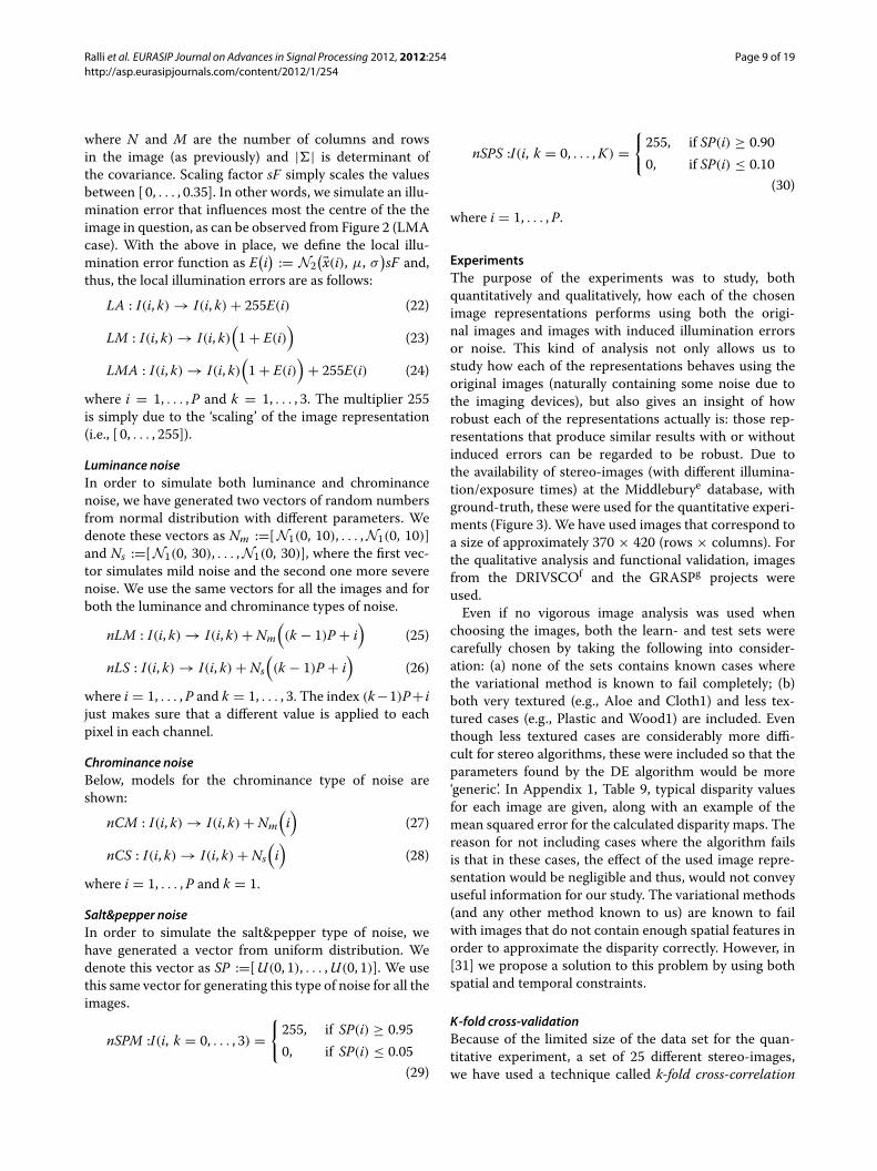
where N and M are the number of columns and rowsin the image (as previously) and || is determinant ofthe covariance. Scaling factor sF simply scales the valuesbetween [ 0, . . . , 0.35]. In other words, we simulate an illu-mination error that influences most the centre of the theimage in question, as can be observed from Figure 2 (LMAcase). With the above in place, we define the local illu-mination error function as E

(i):= N2

(�x(i), μ, σ)sF and,

thus, the local illumination errors are as follows:LA : I(i, k) → I(i, k) + 255E(i) (22)

LM : I(i, k) → I(i, k)(1 + E(i)

)(23)

LMA : I(i, k) → I(i, k)(1 + E(i)

)+ 255E(i) (24)

where i = 1, . . . ,P and k = 1, . . . , 3. The multiplier 255is simply due to the ‘scaling’ of the image representation(i.e., [ 0, . . . , 255]).

Luminance noiseIn order to simulate both luminance and chrominancenoise, we have generated two vectors of random numbersfrom normal distribution with different parameters. Wedenote these vectors as Nm :=[N1(0, 10), . . . ,N1(0, 10)]and Ns :=[N1(0, 30), . . . ,N1(0, 30)], where the first vec-tor simulates mild noise and the second one more severenoise. We use the same vectors for all the images and forboth the luminance and chrominance types of noise.

nLM : I(i, k) → I(i, k) + Nm((k − 1)P + i

)(25)

nLS : I(i, k) → I(i, k) + Ns((k − 1)P + i

)(26)

where i = 1, . . . ,P and k = 1, . . . , 3. The index (k−1)P+ ijust makes sure that a different value is applied to eachpixel in each channel.

Chrominance noiseBelow, models for the chrominance type of noise areshown:

nCM : I(i, k) → I(i, k) + Nm(i)

(27)

nCS : I(i, k) → I(i, k) + Ns(i)

(28)

where i = 1, . . . ,P and k = 1.

Salt&pepper noiseIn order to simulate the salt&pepper type of noise, wehave generated a vector from uniform distribution. Wedenote this vector as SP :=[U(0, 1), . . . ,U(0, 1)]. We usethis same vector for generating this type of noise for all theimages.

nSPM :I(i, k = 0, . . . , 3) ={255, if SP(i) ≥ 0.950, if SP(i) ≤ 0.05

(29)

nSPS :I(i, k = 0, . . . ,K) ={255, if SP(i) ≥ 0.900, if SP(i) ≤ 0.10

(30)

where i = 1, . . . ,P.

ExperimentsThe purpose of the experiments was to study, bothquantitatively and qualitatively, how each of the chosenimage representations performs using both the origi-nal images and images with induced illumination errorsor noise. This kind of analysis not only allows us tostudy how each of the representations behaves using theoriginal images (naturally containing some noise due tothe imaging devices), but also gives an insight of howrobust each of the representations actually is: those rep-resentations that produce similar results with or withoutinduced errors can be regarded to be robust. Due tothe availability of stereo-images (with different illumina-tion/exposure times) at the Middleburye database, withground-truth, these were used for the quantitative experi-ments (Figure 3). We have used images that correspond toa size of approximately 370 × 420 (rows × columns). Forthe qualitative analysis and functional validation, imagesfrom the DRIVSCOf and the GRASPg projects wereused.Even if no vigorous image analysis was used when

choosing the images, both the learn- and test sets werecarefully chosen by taking the following into consider-ation: (a) none of the sets contains known cases wherethe variational method is known to fail completely; (b)both very textured (e.g., Aloe and Cloth1) and less tex-tured cases (e.g., Plastic and Wood1) are included. Eventhough less textured cases are considerably more diffi-cult for stereo algorithms, these were included so that theparameters found by the DE algorithm would be more‘generic’. In Appendix 1, Table 9, typical disparity valuesfor each image are given, along with an example of themean squared error for the calculated disparity maps. Thereason for not including cases where the algorithm failsis that in these cases, the effect of the used image repre-sentation would be negligible and thus, would not conveyuseful information for our study. The variational methods(and any other method known to us) are known to failwith images that do not contain enough spatial features inorder to approximate the disparity correctly. However, in[31] we propose a solution to this problem by using bothspatial and temporal constraints.

K-fold cross-validationBecause of the limited size of the data set for the quan-titative experiment, a set of 25 different stereo-images,we have used a technique called k-fold cross-correlation


Figure 3 Stereo-images from the Middlebury database used in the quantitative experiments. (a) Aloe; (b) Art; (c) Baby1; (d) Baby2; (e)Baby3; (f) Books; (g) Bowling; (h) Cloth1; (i) Cloth2; (j) Cloth3; (k) Cones; (l) Dolls; (m) Lampshade1; (n) Lampshade2; (o) Laundry; (p)Moebius; (q)Plastic; (r) Reindeer; (s) Rocks1; (t) Rocks2; (u) Teddy; (v) Tsukuba; (w) Venus; (x)Wood1; (y)Wood2.

[32,33] to statistically test how well the obtained resultsare generalisable. In our case, due to the size of the dataset, we use a 5-fold cross-correlation: the data set is bro-ken in five sets, each containing five images. Then, werun the DE and analyse the results five times using threeof the sets for learning, one for validation, and one fortesting. In each run the sets for learning, validation andtesting will be different. Results are based on all of thefive runs. Below, there is a list of sets for the first run(Table 4).Information related to the image sets for all the different

runs can be found in Appendix 1, Table 8.

ErrormetricThe error metric that we have used is the mean squarederror (MSE), defined by:

MSE := 1SP

S∑j=1

P∑i=1

((di)j − (dgti)j

)2(31)

where d is the calculated disparity map, dgt is the groundtruth, P is the number of pixels, and S is the number ofimages in the set (e.g., for a single image S = 1) for whichthe mean squared error is to be calculated for.

Table 4 Learn-, validation-, and test sets

Run Learn Test Validation

1 Lampshade2 Cloth1 Rocks2 Aloe Bowling2

Baby3 Reindeer Baby2 Baby1 Laundry

Cones Plastic Tsukuba Books Moebius

Art Wood1 Rocks1 Lampshade1 Venus

Dolls Cloth3 Cloth2 Wood2 Teddy


ResultsIn this section, we present the results, both quantity andvisual quality-wise. First, the results are given by rank-ing how well each representation has done, both accu-racy and robustness-wise. Then, we study how combiningdifferent representations has affected the accuracy andthe robustness of these combined representations. Afterthis, we present the results for some real applications

visual quality-wise, since ground-truth is not available forthese cases.

RankingHere, we rank each of the representation spaces in orderto gain a better insight on the robustness and accuracy ofeach representation. By robustness and accuracy, wemeanthe following: (a) a representation is considered robust

Table 5 Ranking for combined error+noise and original images

Rank Error+ noise MSE Original images MSE

1. ∇ I+PHASE 72.3 ∇ I+HS(V) 35.1

2. ∇ I 83.6 HS(V)+LOGD 37.5

3. PHASE+|∇ I| 84.1 ∇ I+RGB 39.0

4. ∇ I+LOGD 87.4 ∇ I+RGBn 39.4

5. PHASE 92.3 HS(V)+PHASE 40.6

6. (r)φθ+PHASE 92.4 (r)φθ+PHASE 42.2

7. ∇ I+|∇ I| 92.6 ∇ I 44.9

8. RGBn+LOGD 92.8 ∇ I +LOGD 45.6

9. LOGD 97.5 ∇ I+PHASE 46.0

10. RGB+PHASE 102.7 RGB+LOGD 46.0

11. LOGD+|∇ I| 105.5 RGBn+LOGD 46.8

12. RGBn+|∇ I| 111.5 RGBn+PHASE 47.1

13. HS(V)+|∇ I| 112.0 PHASE+|∇ I| 47.7

14. RGB+|∇ I| 112.9 RGB+PHASE 47.9

15. ∇ I+RGBn 114.8 PHASE 48.3

16. RGBn+PHASE 120.0 LOGD 50.7

17. HS(V)+PHASE 120.2 HS(V)+(r)φθ 53.2

18. RGB+LOGD 125.7 (r)φθ 53.6

19. ∇ I+(r)φθ 134.1 LOGD+|∇ I| 55.2

20. (r)φθ+|∇ I| 139.8 HS(V)+|∇ I| 55.9

21. ∇ I+RGB 175.0 (r)φθ+|∇ I| 56.9

22. ∇ I+HS(V) 180.4 RGB+|∇ I| 57.7

23. HS(V)+LOGD 278.4 ∇ I+|∇ I| 59.8

24. HS(V) 293.8 RGBn+|∇ I| 62.1

25. RGB+HS(V) 360.8 RGBn+HS(V) 74.8

26. RGBn+HS(V) 373.8 ∇ I+(r)φθ 99.3

27. RGBn 374.4 (r)φθ+LOGD 103.7

28. RGB 380.7 RGB+(r)φθ 119.4

29. RGB+RGBn 394.3 HS(V) 134.3

30. (r)φθ+LOGD 394.8 RGBn+(r)φθ 166.3

31. HS(V)+(r)φθ 563.8 RGB+HS(V) 178.8

32. (r)φθ 712.2 RGB 224.8

33. RGBn+(r)φθ 716.7 RGB+RGBn 239.1

34. RGB+(r)φθ 727.4 RGBn 260.3

Combined error+noise is MSE of all the different illumination errors and noise types.


when results based on it are affected only slightly by noiseor image errors; (b) a representation is considered accu-rate when results based on this gives good results usingthe original (i.e., noiseless) images. While this may not bethe standard terminology, we find that using these termsmakes it easier to explain the results. In Table 5, eachof the representations is ranked with respect to (a) the

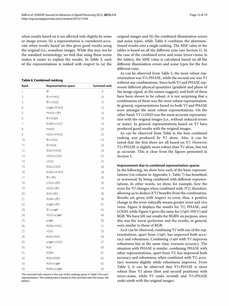
Table 6 Combined ranking

Rank Representation space Summed rank

1. ∇ I 9

2. ∇ I+PHASE 10

3. ∇ I+LOGD 12

4. (r)φθ+PHASE 12

5. PHASE+|∇ I| 16

6. ∇ I+RGBN 19

7. RGBN+LOGD 19

8. PHASE 20

9. HS(V)+PHASE 22

10. ∇ I+HS(V) 23

11. ∇ I+RGB 24

12. RGB+PHASE 24

13. HS(V)+LOGD 25

14. LOGD 25

15. RGB+LOGD 28

16. RGBN+PHASE 28

17. ∇ I+|∇ I| 30

18. LOGD+|∇ I| 30

19. HS(V)+|∇ I| 33

20. RGB+|∇ I| 36

21. RGBN+|∇ I| 36

22. (r)φθ+|∇ I| 41

23. ∇ I+(r)φθ 45

24. HS(V)+(r)φθ 48

25. (r)φθ 50

26. RGBN+HS(V) 51

27. HS(V) 53

28. RGB+HS(V) 56

29. (r)φθ+LOGD 57

30. RGB 60

31. RGBN 61

32. RGB+RGBN 62

33. RGB+(r)φθ 62

34. RGBN+(r)φθ 63

The summed rank column is the sum of the rankings given in Table 5 for eachrepresentation. The ranking here is based on the summed rank (the lower, thebetter).

original images and (b) the combined illumination errorsand noise types, while Table 6 combines the aforemen-tioned results into a single ranking. The MSE value in thetables is based on all the different runs (see Section 1). Inthe case of the combined error and noise (error+noise inthe tables), the MSE value is calculated based on all thedifferent illumination errors and noise types for the fivedifferent runs.As can be observed from Table 5, the most robust rep-

resentation was ∇I+PHASE, while the second one was ∇Iwithout any combinations. Since both∇I and PHASE rep-resent different physical quantities (gradient and phase ofthe image signal, as the names suggest), and both of thesehave been shown to be robust, it is not surprising that acombination of these was the most robust representation.In general, representations based on both ∇I and PHASEwere amongst the most robust representations. On theother hand, ∇I+LOGDwas the most accurate representa-tion with the original images (i.e., without induced errorsor noise). In general, representations based on ∇I haveproduced good results with the original images.As can be observed from Table 6, the best combined

ranking was produced by ∇I alone. Also, it can benoted that the first three are all based on ∇I. However,∇I+PHASE is slightly more robust than ∇I alone, but notas accurate. This is clear from the figures presented inSection 1.

Improvement due to combined representation spacesIn the following, we show how each of the basic represen-tations (1st column in Appendix 1, Table 7) has benefited,or worsened, by being combined with different represen-tations. In other words, we show, for example, how theerror for ∇I changes when combined with |∇I|, therefore,allowing us to deduce if∇I benefits from the combination.Results are given with respect to error, thus, a positivechange in the error naturally means greater error and viceversa. Figure 4 displays the results for ∇I, PHASE, andLOGD, while Figure 5 gives the same for (r)φθ , HS(V) andRGB.We have left out results for RGBN on purpose, sincethis was the worst performer and the results, in general,were similar to those of RGB.As it can be observed, combining∇I with any of the rep-

resentations, apart from (r)φθ , has improved both accu-racy and robustness. Combining (r)φθ with ∇I improvesrobustness but at the same time, worsens accuracy. Thesituation with PHASE is similar: combining PHASE withother representations, apart from ∇I, has improved bothaccuracy and robustness; when combined with ∇I, accu-racy worsens slightly while robustness improves. FromTable 5, it can be observed that ∇I+PHASE is morerobust than ∇I alone (first and second positions) witherror+noise, while ∇I ranks seventh and ∇I+PHASEranks ninth with the original images.


Figure 4 Change in error due to combined representation. Results for ∇ I, PHASE, and LOGD. A positive value indicates an increase in error, whilea negative value indicates a decrease in error.

Visual qualitative interpretationFigures 6, 7, and 8 display results visually for the Cones,DRIVSCO, and GRASP cases, using the following imagerepresentations:∇I,∇I+PHASE, ∇I+HS(V), PHASE, andRGB. A video of the results for DRIVSCO is available ath.These representations were chosen since (a) ∇I was theoverall ‘winner’ for the combined results (see Table 6);(b) ∇I+PHASE was the most robust one; (c) ∇I+HS(V)was the most accurate one; (d) PHASE is both robust andaccurate, and (e) RGB is the ‘standard’ representation fromtypical cameras. The parameters used were the same inall the cases presented here and are those from the 1strun (out of five) for the 5-fold cross-validation. The rea-soning here is, confirmed by the results, that any robust

representation should be able to generate reasonableresults for any of the parameters found in the cross-validation scheme.As can be observed from Figure 6, the results are some-

what similar for all the representations. However, as it canbe observed, RGB has visually produced slightly worseresults.Figure 7 shows results for the DRIVSCOi sequence

(Additional file 1). Here, ∇I+PHASE has produced themost concise results: results for the road are far betterthan with any of the other representations. On the otherhand, ∇I+HS(V) has produced the best results for thetrailer: obtaining correct approximations for the trailer ischallenging since it tends to ‘fuse’ with the trees. RGB


Figure 5 Change in error due to combined representation. Results for (r)φθ , HS(V), and RGB. A positive value indicates an increase in error, whilea negative value indicates a decrease in error.

has produced very low quality results and, for example,scene interpretation based on these results would be verychallenging if not impossible.Figure 8 shows results for a robotic grasping scene. Both

∇I and ∇I+HS(V) have produced good results: the objectof interest lying on the table is recognisable in the dis-parity map. ∇I+PHASE or PHASE alone has increased‘leakage’ of disparity values between the object of interestand the shelf. On the other hand, PHASE representa-tion has produced the best results for the table, espe-cially for the lowest part. Again, RGB has produced lowquality results.Altogether, visual qualitative interpretation of the

results using real image sequences is in line with the

quantitative analysis. Both ∇I and ∇I+PHASE producegood results even with real image sequences. However, theformer produces slightly more accurate results while thelatter representation is more robust.

ConclusionsWe have shown that the quality of a disparity map, gener-ated by a variational method, under illumination changesand image noise, depends significantly on the used imagerepresentation type. By combining different representa-tions, we have generated and tested 34 different cases andfound several complementary spaces that are affected onlyslightly even under severe illumination errors and imagenoise. Accuracy differences of 7-fold (without noise) and


Figure 6 Cones. (a) Ground truth; (b) ∇ I; (c) ∇ I+PHASE; (d) ∇ I+HS(V); (e) PHASE; (f) RGB.

Figure 7 DRIVSCO scene. (a) Left image; (b) ∇ I; (c) ∇ I+PHASE; (d) ∇ I+HS(V); (e) PHASE; (f) RGB.

Figure 8 GRASP scene. (a) Left image; (b) ∇ I; (c) ∇ I+PHASE; (d) ∇ I+HS(V); (e) PHASE; (f) RGB.


10-fold (with noise and illumination errors) were foundbetween the best and worst representation maps, whichhighlights the relevance of an appropriate input repre-sentation for low level estimations such as stereo. Thisaccuracy enhancing and robustness to noise can be ofcritical importance in specific application scenarios withreal uncontrolled scenes and not just well behaving testimages (e.g., automatic navigation, advanced robotics,CGI). Amongst the tested combinations, the ∇I represen-tation stood out as one of the most accurate and leastaffected by illumination errors or noise. By combining∇I with PHASE, the joined representation space was themost robust one amongst the tested spaces. This findingwas also confirmed by the qualitative experiments. Thus,we can say that the aforementioned representations com-plement each other. These results were also confirmed ina qualitative evaluation of natural scenes in uncontrolledscenarios.There are some studies similar to ours, carried out in

a smaller scale. However, the other studies typically pro-vide little information related to how the optimum (ornear optimum) parameters of the algorithm are achieved,related to each representation space: in this study, we haveused a well known, derivative free, stochastic algorithmcalled DE for the reasons given in the text. We argue thatmanually obtained parameters are subjected to a bias fromthe human operator and therefore, can be expected toconfirm expected results. Three different sets of imageswere used for obtaining the parameters and testing eachof the representations, in order to avoid over-fitting. Theproposed methodology for estimating model parameterscan be extended to many other computer vision algo-rithms. Therefore, our contribution should lead to morerobust computer vision systems capable of working withreal applications.

Future studyThe weighting factors (b1 and b2 in (1)) for each imagerepresentation are applied equally to all of the ‘channels’.

Since some of the channels are more robust than others,like in the case of HSV for example, each channel shouldhave its own weighting factor. Since this study allows us tocut down the number of useful representations, we pro-pose to study the best behaving ones in more detail withseparate weighting factors where needed.

Appendix 1Image representations and setsTypical disparity valuesThe following table displays minimum, maximum, mean,and standard deviation (STD) of ground-truth disparityfor each of the used images. Also, in the same table wegive theMSE (mean squared error), for each of the images,calculated using the parameters from the 1st run for the∇I based image representation. The lowest numbers arethe mean, standard deviation and MSE for the wholeimage set. The number on the lowest row in the tableare the mean, standard deviation and MSE for the wholeimage set.As it can be observed from Table 9, for some of the

images the MSE is some what big. This does not comeas a complete surprise since some of the images, such asWood1, Wood2, Lampshade1, and Lampshade2 containonly few useful spatial features for approximating the dis-parity correctly. As future study, it would be interesting todivide the images into two categories (ones with sufficientspatial features and ones with only very few spatial fea-tures), and then search for the optimum parameters usingthe DE algorithm. Now, if there would be considerableimprovement in either of the sets, then this would suggestthat the parameters should be chosen based on previousimage analysis step.

Endnotesahttp://www.jarnoralli.fi/.bhttp://www.icsi.berkeley.edu/∼storn/code.html.chttp://vision.middlebury.edu/stereo/data/.dhttp://vision.middlebury.edu/stereo/data/.

Table 7 Tested image representation combinations

Term Term

None RGB RGBN |∇I| HS(V) (r)φθ Phase LOGD

None

RGB X X X X X X X

RGBN X X X X X X

∇ I X X X X X X X X

HS(V) X X X X X

(r)φθ X X X X

Phase X X

LOGD X X

http://www.jarnoralli.fi/

http://www.icsi.berkeley.edu/~storn/code.html

http://vision.middlebury.edu/stereo/data/



Table 8 Learn-, validation-, and test sets

Run Learn Test Validation

1 Lampshade2 Cloth1 Rocks2 Aloe Bowling2

Baby3 Reindeer Baby2 Baby1 Laundry

Cones Plastic Tsukuba Books Moebius

Art Wood1 Rocks1 Lampshade1 Venus

Dolls Cloth3 Cloth2 Wood2 Teddy

2 Baby1 Cloth1 Teddy Art Rocks1

Aloe Wood1 Reindeer Baby2 Rocks2

Lampshade1 Laundry Bowling2 Cloth3 Cloth2

Dolls Wood2 Lampshade2 Plastic Books

Cones Baby3 Moebius Tsukuba Venus

3 Aloe Rocks1 Lampshade1 Baby1 Baby3

Dolls Venus Moebius Bowling2 Wood2

Laundry Tsukuba Rocks2 Lampshade2 Plastic

Cones Baby2 Books Reindeer Cloth2

Wood1 Art Cloth3 Teddy Cloth 1

4 Baby3 Cones Tsukuba Baby1 Books

Rocks2 Art Cloth3 Cloth2 Lampshade2

Laundry Dolls Reindeer Teddy Cloth1

Plastic Bowling2 Lampshade1 Venus Rocks1

Aloe Wood2 Baby2 Wood1 Moebius

5 Bowling2 Books Reindeer Baby2 Teddy

Tsukuba Cloth3 Rocks2 Cloth1 Baby3

Moebius Aloe Laundry Plastic Venus

Cones Wood1 Art Rocks1 Cloth2

Lampshade1 Dolls Lampshade2 Wood2 Baby1

Table 9 Typical disparity values for each image, andMSE for each image using parameters from the 1st run for∇Iimage representation

Image Min Max Mean Std MSE

Aloe 14.33 70.33 24.13 9.34 43.7

Art 24.33 74.67 44.36 14.37 95.5

Baby1 8.33 45.33 27.79 10.66 24.6

Baby2 13.33 51.67 28.95 12.05 7.8

Baby3 15.67 51.00 42.15 6.93 11.7

Books 21.67 73.67 43.00 14.71 8.7

Bowling2 13.33 66.00 46.88 15.96 116.0

Cloth1 13.00 57.33 38.28 8.93 0.6

Cloth2 14.00 76.00 53.24 12.37 30.6

Cloth3 15.00 55.33 36.28 11.31 5.1

Cones 5.50 55.00 33.54 11.58 8.7

Dolls 3.00 73.67 45.85 14.09 4.2

Lampshade1 14.00 64.67 35.87 15.90 78.2

Lampshade2 8.67 65.33 38.92 14.46 75.5


Table 9 Typical disparity values for each image, andMSE for each image using parameters from the 1st run for∇Iimage representation (continued)

Laundry 11.67 77.33 40.29 12.95 27.3

Moebius 21.33 72.67 37.19 11.20 12.7

Plastic 7.67 65.33 45.27 13.36 15.4

Reindeer 3.67 67.00 41.54 15.01 112.8

Rocks1 19.33 56.67 37.53 9.50 1.7

Rocks2 23.33 56.00 38.57 7.00 1.3

Teddy 12.50 52.75 27.38 9.02 8.8

Tsukuba 5.00 14.00 6.79 2.67 2.1

Venus 3.00 19.75 8.89 4.09 1.0

Wood1 21.67 71.67 40.83 12.71 102.5

Wood2 14.33 72.33 48.89 15.46 126.6

37.08 15.82 36.9

ehttp://vision.middlebury.edu/stereo/data/.fhttp://www.pspc.dibe.unige.it/∼drivsco/.ghttp://www.csc.kth.se/grasp/.hhttp://www.jarnoralli.fi/.ihttp://www.jarnoralli.fi/joomla/publications/representation-space.

Additional file

Additional file 1: DRIVSCO sequence disparity results. Disparitycalculation results for the DRIVSCO sequence using different imagerepresentations.

Competing interestsThe authors declare that they have no competing interests.

AcknowledgementsWe thank Dr. Javier Sanchez and Dr. Luis Alvarez from the University of LasPalmas de Gran Canaria, and Dr. Stefan Roth from the technical University ofDarmstadt for helping us out getting started with the variational methods.Further, we would like to thank Dr. Andres Bruhn for our fruitful conversationsduring the DRIVSCO workshop 2009. Also, we would like to thank the PDCCenter for High Performance Computing of Royal Institute of Technology(KTH, Sweden) for letting us use their clusters. This work was supported by theEU research project TOMSY (FP7-270436), the Spanish Grants DINAM-VISION(DPI2007-61683) and RECVIS (TIN2008-06893-C03-02), Andalusia’s regionalprojects (P06-TIC-5060 and TIC-3873) and Granada Excellence Network ofInnovation Laboratories’ project PYR-2010-19.

Received: 16 September 2011 Accepted: 13 November 2012Published: 10 December 2012

References1. BKP Horn, BG Schunck, Determining optical flow. Artif. Intell. 17, 185–203

(1981)2. Y Huang, K Young, Binocular image sequence analysis: integration of

stereo disparity and optic flow for improved obstacle detection andtracking. EURASIP J. Adv. Signal Process. 2008, 10 (2008)

3. M Bjorkman, D Kragic, in Proceedings of the British Machine VisionConference. Active 3D segmentation through fixation of previously unseenobjects (BMVA Press, 2010), pp. pp. 119.1–119.11. doi:10.5244/C.24.119

4. Y Mileva, A Bruhn, J Weickert, in DAGM07- Volume LNCS, vol. 4713.Illumination-robust variational optical flow with photometric invariants(Heidelberg, Germany, 2007), pp. 152–162

5. C Wohler, P d’Angelo, Stereo image analysis of non-lambertian surfaces.Int. J. Comput. Vision. 81(2), 172–190 (2009)

6. B Maxwell, R Friedhoff, C Smith, in in IEEE Conference on Computer Visionand Pattern Recognition (CVPR 2008). A bi-illuminant dichromatic reflectionmodel for understanding images (Anchorage, Alaska, USA, 2008), pp. 1–8

7. S Shafer, Using color to separate reflection components. Tech. rep (1984).[TR 136, Computer Science Department, University of Rochester]

8. DG Lowe, Distinctive image features from scale-invariant keypoints. Int. J.Comput. Vision. 60, 91–110 (2004)

9. H Bay, A Ess, T Tuytelaars, LV Gool, Speeded-up robust features (SURF).Comput. Vis. Image Underst. 110, 346–359 (2008)

10. A Bruhn, Variational optic flow computation: accurate modelling andefficient numerics. PhD thesis, Saarland University, Saarbrucken, Germany(2006)

11. T Brox, From pixels to regions: partial differential equations in imageanalysis. PhD thesis, Saarland University, Saarbrucken, Germany (2005)

12. A Bruhn, J Weickert, T Kohlberger, C Schnorr, A multigrid platform forreal-time motion computation with discontinuity-preserving variationalmethods. Int. J. Comput. Vision. 70(3), 257–277 (2006)

13. N Slesareva, A Bruhn, J Weickert, in DAGM05- Volume LNCS 3663. Optic flowgoes stereo: a variational method for estimating discontinuity-preservingdense disparity maps (Vienna, Austria, 2005), pp. 33–40

14. T Brox, A Bruhn, N Papenberg, J Weickert, in ECCV04-Volume LNCS 3024.High accuracy optical flow estimation based on a theory for warping(Prague, Czech Republic, 2004), pp. 25–36

15. M Black, P Anandan, in Proc. Computer Vision and Pattern Recognition.Robust dynamic motion estimation over time (Maui, Hawaii, USA, 1991),pp. 296–302

16. J Weickert, C Schnorr, A theoretical framework for convex regularizers inPDE-based computation of image motion. Int. J. Comput. Vision. 45(3),245–264 (2001)

17. H Nagel, W Enkelmann, An investigation of smoothness constraints forthe estimation of displacement vector fields from image sequences.PAMI. 8(5), 565–593 (1986)

18. L Alvarez, J Weickert, J Sanchez, Reliable estimation of dense optical flowfields with large displacements. Int. J. Comput. Vision. 39, 41–56(2000)

19. H Zimmer, A Bruhn, J Weickert, L Valgaerts, A Salgado, B Rosenhahn, HSeidel, in EMMCVPR , vol. 5681 of Lecture Notes in Computer Science.Complementary optic flow (Bonn, Germany, 2009), pp. 207–220

20. A Blake, A Zisserman, Visual Reconstruction. (The MIT Press, Cambridge,Massachusetts London, England, 1987)

21. U Trottenberg, C Oosterlee, A Schuller,Multigrid, (Academic Press, AHarcourt Science and Technology Company Harcourt Place. 32Jamestown Road, London NW1 7BY UK, 2001)

22. R Storn, K Price, Differential evolution—a simple and efficient adaptivescheme for global optimization over continuous spaces. Tech. rep (1995).[TR-95-012, ICSI]


http://www.pspc.dibe.unige.it/~drivsco/

http://www.csc.kth.se/grasp/

http://www.jarnoralli.fi/

http://www.jarnoralli.fi/joomla/publications/representation-space

http://www.jarnoralli.fi/joomla/publications/representation-space

http://www.biomedcentral.com/content/supplementary/1687-6180-2012-254-S1.flv

http://dx.doi.org/10.5244/C.24.119


23. R Storn, K Price, Differential evolution—a simple, efficient heuristic forglobal optimization over continuous spaces. J. Global Optimiz. 11(4),341–359 (1997)

24. VP Plagianakos, MN Vrahatis, Parallel evolutionary training algorithms forhardware-friendly neural networks. Nat. Comput. 1, 307–322 (2002)

25. DK Tasoulis, N Pavlidis, VP Plagianakos, MN Vrahatis, in In IEEE Congress onEvolutionary Computation (CEC). Parallel differential evolution, (Portland,OR, USA, 2004), pp. 1–6

26. MG Epitropakis, VP Plagianakos, MN Vrahatis, Hardware-friendlyhigher-order neural network training using distributed evolutionaryalgorithms. Appl. Soft Comput. 10, 398–408 (2010)

27. D Hubel, T Wiesel, Anatomical demonstration of columns in the monkeystriate cortex. Nature. 221, 747–750 (1969)

28. D Fleet, A Jepson, Stability of phase information. IEEE Trans. Pattern Anal.Mach. Intell. 15(12), 1253–1268 (1993)

29. D Fleet, A Jepson, Phase-based disparity measurement. Comput. VisionGraphics Image Process. 53(2), 198–210 (1991)

30. S Sabatini, G Gastaldi, F Solari, K Pauwels, MV Hulle, Jx Dıaz, J Ros, NPugeault, N Kruger, A compact harmonic code for early vision based onanisotropic frequency channels. Comput. Vis. Image Underst. 114,681–699 (2010)

31. J Ralli, J Dıaz, E Ros, Spatial and temporal constraints in variationalcorrespondence methods. Mach. Vision Appl, 1–13 (2011)

32. PA Devijver, J Kittler, Pattern Recognition: a Statistical Approach. (PrenticeHall, 1982). ISBN 13: 9780136542360, ISBN 10: 0136542360

33. R Kohavi, in Proceedings of the 14th International Joint Conference onArtificial Intelligence- Volume 2. A study of cross-validation and bootstrapfor accuracy estimation and model selection, (Morgan Kaufmann,Montreal, Quebec, Canada, 1995), pp. 1137–1143

doi:10.1186/1687-6180-2012-254Cite this article as: Ralli et al.: Experimental study of image representationspaces in variational disparity calculation. EURASIP Journal on Advances inSignal Processing 2012 2012:254.

Submit your manuscript to a journal and benefi t from:

7 Convenient online submission

7 Rigorous peer review

7 Immediate publication on acceptance

7 Open access: articles freely available online

7 High visibility within the fi eld

7 Retaining the copyright to your article

Submit your next manuscript at 7 springeropen.com

Experimental study of image representation spaces in variational disparity calculation

Documents

Transcript of Experimental study of image representation spaces in variational disparity calculation