1

+. EXPERIMENTAL STUDY OF A FREE TURBULENT SHEAR FLOW AT MACH 19 WITH ELECTRON-BEAM AND CONVENTIONAL PROBE$

William D. Harvey and Wil/iam W. Hzlnter, Jr.,i I

Langley Research Center Humpton, Vu. 23665

3. 5 4

N A T I O N A L AERONAUTICS A N D SPACE ADM-M W A S H I N G T O N , D. C. OCT&BR W5

e

https://ntrs.nasa.gov/search.jsp?R=19750024313 2020-03-20T17:12:15+00:00Z

I I I I

- -

TECH LIBRARY KAFB, NM

_- ~

1. Report No. 2. Government Accession No.

NASA T N D-7981 I 4. Title and Subtitle

EXPERIMENTAL STUDY OF A F R E E TURBULENT SHEAR FLOW AT MACH 19 WITH ELECTRON-BEAM AND CONVENTIONAL PROBES

7. Author(s)

Will iam D. Harvey and Wil l iam W. Hunter, Jr.

9. Performing Organization Name and Address

NASA Langley R e s e a r c h Cen te r Hampton, Va. 23665

2. Sponsoring Agency Name and Address

National Aeronaut ics and Space Adminis t ra t ion Washington, D.C. 20546

5. Supplementary Notes

Illllllllll1 Ill1Ulll Ill__ ... 0133538

3. Recipient's Catalog No.

5. Report Date

October 1975 6. Performing Organization Code

8. Performing Organization Report No.

L-10138 10. Work Unit No.

505-06 -4 1-01

11. Contract or Grant No.

13. Type of Report and Period Covered

Technica l Note

14. Sponsoring Agency Code

Appendix by Wil l iam W. Hunter, Jr., and J a m e s I. Clemmons , Jr.

.. . ~

6. Abstract

An expe r imen ta l study of the ini t ia l development r eg ion of a hype r son ic turbulent free mixing l a y e r h a s been made. Da ta w e r e obtained at t h r e e s t a t i o n s downs t r eam of a M = 19 nozz le ove r a Reynolds r a n g e of 1.3 X lo6 t o 3.3 X 106 p e r m e t e r (4.0 X lo5 t o 9.2 X 105 p e r foot) and at a total t e m p e r a t u r e of about 1670 K (3000O R). In gene ra l , good ag reemen t w a s obtained between e l ec t ron -beam and conventional p robe m e a s u r e m e n t s of l oca l m e a n flow p a r a m e t e r s . Measuremen t s of f luctuat ing densi ty indicated tha t peak roo t -mean- squa re ( r m s ) l e v e l s are higher in the turbulent free mixing l a y e r t han in boundary l a y e r s f o r Mach n u m b e r s less than 9. The intensi ty of r m s densi ty f luctuat ions in t h e free s t r e a m is s i m i l a r in magni tude t o p r e s s u r e f luctuat ions in high Mach number flows. Spec t rum ana lyses of t he m e a s u r e d fluctuating densi ty through the s h e a r l aye r indicate s ignif icant f luctuation ene rgy at the lower f r equenc ie s (0.2 t o 5 kHz) which co r re spond t o l a r g e - s c a l e d i s t u r b a n c e s in the high-velocity r eg ion of t he s h e a r l aye r .

7. Key-Words (Suggested by Author(s))

E l e c t r o n beam Conventional p r o b e s Free s h e a r flow

9. Security Classif. (of this report)

Unclass i f ied

18. Distribution Statement

Unclass i f ied - Unlimited

Subject Category 34

20. Security Classif. (of this page)

Unclass i f ied

For Sale by the National Technical Information Service, Springfield, Virginia 22161

EXPERIMENTALSTUDYOFAFREETURBULENTSHEARFLOWAT

MACH 19 WITH ELECTRON-BEAM AND CONVENTIONAL PROBES

William D. Harvey and William W. Hunter, Jr. Langley Research Center

SUMMARY

An experimental study of the initial development region of a hypersonic turbulent free mixing layer has been made. Data were obtained at three stations downstream of a M = 19 nozzle over a Reynolds range of 1.3 X lo6 to 3.3 X lo6 per meter (4.0 X lo5 to 9.2 x lo5 per foot) and at a total temperature of about 1670 K (3000O R). In general, good agreement was obtained between electron-beam and conventional probe measure­ments of local mean flow parameters. Measurements of fluctuating density indicated that peak root-mean-square (rms) levels a r e higher in the turbulent free mixing layer than in boundary layers for Mach numbers l e s s than 9. The intensity of r m s density fluctuations in the f r e e s t ream is similar in magnitude to pressure fluctuations in high Mach number flows. Spectrum analyses of the measured fluctuating density through the shear layer indicate significant fluctuation energy at the lower frequencies (0.2 to 5 kHz) which corre­spond to large-scale disturbances in the high-velocity region of the shear layer.

INTRODUCTION

One of the more important results of the recent Conference on F r e e Turbulent Shear Flows (ref. 1) held at Langley Research Center was the identification of inconsistent free shear layer data that are taken in the initial development region of a shear layer o r in transitional flows rather than in fully developed turbulent flows. Reference 1 provides a n excellent review of the state of the art in turbulent f r ee shear layer flows. In reference 2 the importance of developing accurate calculation methods for turbulent free mixing layers and the concomitant need for accurate experimental data were pointed out. The effects of Mach number and Reynolds number on spreading rates in fully developed turbulent flow are ill-defined; these effects are uncertain because of insufficient experimental data. In addition, turbulence measurements in supersonic and hypersonic shear layers are required before adequate theories can be developed.

Recent measurements have been obtained of mean and turbulence flow quantities in a Mach 5 nozzle shear layer (ref. 3) where the test Reynolds numbers were in the range required to achieve fully developed turbulent flow. These Mach 5 results show the

spreading rate of fully developed shear layers to be considerably lower than those fo r previous subsonic data. Furthermore, a corresponding reduction in the velocity fluctua­tion intensity across the shear layer was obtained from hot-wire surveys. Mean profile data in the initial development region of a hypersonic shear layer are presented in refer­ence 4 for a single station about 13 cm (5.25 in.) downstream of the exit of a Mach 19.5 nozzle where the nozzle-wall turbulent boundary layer was 10 cm (4 in.) thick at the exit. Estimates indicate that distances downstream from the exit of the Mach 19.5 nozzle (ref. 4)on the order of 12 boundary-layer thicknesses would be required to achieve self-s imilar turbulent flow profiles.

The purpose of the present study is to investigate the initial development region of a hypersonic f r ee shear layer by the analysis of mean profile data at several longitudinal stations obtained with both conventional probes and the electron-beam technique. Conven tional probes were used to measure the mean static pressure, pitot pressure, and total temperature profiles. The electron beam was also utilized to measure the mean density and temperature as well as fluctuations in density across the hypersonic turbulent shear layer. The present data a r e believed to be unique in that no other detailed data on the initial development of a hypersonic turbulent f r ee mixing layer at Mach 19 are available.

SYMBOLS

Measurements are presented in SI and U.S. Customary Units. measurements were made in U.S.Customary Units.

A,B,C ,D,E,F,G constants

d v diameter

f frequency

Af frequency bandwidth

current

Calculations and

K coefficient including geometry, optical, and electronic system parameters

M Mach number

N number density

2

I

N;t 1 +

N2X =g

+ 2 + N2B

2 + z g

NR

P

Pt,2

RUJ

RXJ,x ST

T

Tr

t

U

V

X

-X

Y

Y

nitrogen ion

neutral state of nitrogen molecule

excited ionized state of nitrogen molecule

ground ionized state of nitrogen molecule

ratio of photodetector output to total beam current

pressure

pitot pressure

free-stream Reynolds number per unit length at nozzle exit

free-stream Reynolds number based on distance from nozzle exit

measured spectral ratio

temperature

rotational temperature

time

velocity

voltage

longitudinal distance

longitudinal distance from nozzle exit

normal distance from nozzle center line

normal distance from wall boundary or from where u/ue = 0.05 in shear layer

3

boundary-layer o r shear-layer thickness (7 at U/Ue = 0.999 for boundary layer and 0.999 5 u/ue 5 0.05 for shear layer)

mass density

-spreading rate, X

0.5642 +/Ue>

normalized power spectral density,

w wave number, 27rf/u

Subscripts:

a ambient

B test-box conditions

e edge values

settling chamber conditions

t local stagnation conditions

W wall conditions

[V’(fD n

6 boundary- layer o r shear -layer thickness

Bars over symbols denote time mean values and pr imes denote fluctuating values.

APPARATUS AND TESTS

A schematic sketch of the Langley hypersonic nitrogen tunnel and test equipment used in the present experiment is shown in figure 1 (top view of tunnel shown). The flow in the axially symmetrical nozzle exhausts into the vacuum test box. The boundary layer on the nozzle wall at the exit x = 224.8 cm (x = 88.5 in.) is about 10 cm (4 in.) thick. The nozzle was water-cooled in order to maintain a constant wall temperature. The facility can be operated continuously for 2 hours o r more. Preliminary calibrations of

4

0

the flow and techniques of operation a r e given in reference 5. The present tests (table I) were made at a nominal Mach number of 19 in high purity nitrogen (5 par t s per million of oxygen) at a nominal total temperature of about 1670 K (3000' R). The jet f ree-s t ream Reynolds number was varied from about 1.3 X lo6 to 3.3 X lo6 per meter (4 x lo5 to 10 x lo5 per foot). The jet f r ee s t ream is defined as being the inviscid flow region along the nozzle o r jet center line.

Detailed surveys of mean total temperature, pitot pressure, and static pressure were made with conventional probes across the shear-layer region at the nozzle exit and at about 1.3 and 3.5 boundary-layer thicknesses downstream of the exit. The electron-beam technique w a s utilized to measure the mean density and static temperature simul­taneously at about 1.3 boundary-layer thicknesses downstream of the exit. Measurements of total temperature, pitot pressure, and static pressure across the turbulent boundary layer on the nozzle wall, at about 1.6 boundary-layer thicknesses upstream of the exit, are given in reference 6 for about the same flow conditions as presented herein.

INSTRUMENTATION

General

Several methods have been used to measure local flow parameters in nozzle-wall boundary layers and f r ee mixing layers. Conventional probes provide direct measure­ments of pitot pressure, total temperature, and static pressure from which other local parameters may be calculated. However, probe data a r e subject to e r r o r s because of the presence of the turbulence and/or viscous effects. The nonintrusive electron-beam tech­nique has been employed extensively in recent years for direct measurements of density and temperature. (See refs. 7 to 14.) Electron-beam static density and static tempera­ture measurements a r e accomplished by determining the level and spectral distributions of local gas fluorescence resulting from fast electron collisions with molecules and subsequent spontaneous emission. (An extensive bibliography of electron-beam tech-

The electron beam has also been used toniques and results may be found in ref. 10.) measure mean and fluctuating density in a Mach 8.5 nozzle-wall boundary layer (ref. 14) and the initial development region of a hypersonic (Me = 19.5) f ree mixing layer (ref. 4). Most available investigations were limited to s t ream Mach numbers l e s s than 9, and few comparisons of the electron-beam measurements with conventional probe data have been made.

Conventional probes a r e subject to numerous e r r o r s caused by viscous effects o r interference effects. (See ref. 6.) The first step in comparing conventional probe data with electron-beam data must necessarily be on assessment of these probe e r r o r s . How­ever, e r r o r s caused by interference 'effects between the probes and flow a r e difficult to

5

asses s . Since the electron-beam technique provides data free of probe interference effects, the magnitude of such e r r o r s can be estimated if all other sources of e r r o r in both the probe and electron-beam data can be identified and evaluated. A detailed dis­cussion of the electron-beam instrumentation and calibration is given in the appendix by William W. Hunter, Jr., and James I. Clemmons, Jr.

Conventional Survey Probes

Surveys ac ross the axisymmetric shear layer were made with probes supported by a water-cooled s t rut (fig. 1)located on the opposite side of the tunnel f rom the density o r temperature apparatus. The probe measurements were made in a horizontal plane through the center line of the tunnel and the beam measurements were made in a vertical plane through the center line. The probe strut-traversing mechanism (ref. 6) allows the probes to be positioned along or normal to the flow center line to within 0.0254 cm (0.01 in.). Sketches of the probes a r e given as inser t s in figures 2(a) and 3(a). Surveys of mean total temperature, mean pitot pressure, and static pressures were made simul­taneously across the mixing region a t several x-stations. Pitot tubes were 0.3175 cm (0.125 in.) outside diameter stainless-steel tubes which were internally chamfered at the mouth. The static-pressure probes were also constructed of 0.3175-cm-diameter (0.125-in.) tubing with sharp cone tips. The total angle of the conical tips was 35'. Four 0.0787-cm -diameter (0.031-in.) pressure orifices were located 5.08 cm (2 in.) downstream of the cone tip. (See fig. 2.) The orifice locations were determined from inviscid theoretical calculations of the static-pressure distributions along the surface of the probe for the expected Mach number range through the shear layer. (The numerical method used was that of ref. 15.) The pitot- and static-pressure probes have been ana­lyzed for viscous and rarefaction effects (ref. 6) and corrections have been applied where required. Large corrections (about 50 percent maximum) were applied for pitot-pressure data in the low-velocity region of the shear layer, and lesser corrections were applied up to about 15.24 cm (6 in.) approaching the high-velocity region. P res su re transducers of the type described in reference 6 were used for the pitot- and static-pressure measurements.

The sensing element of the total temperature probe (fig. 3(a)) was an alumel wire of 0.0254-cm (0.01-in.) diameter with small 'chromel wires of 0.00762-cm (0.003-in.) diameter attached at the center and at the ends. The small chromel wires attached to the ends of the alumel wire provided measurements of end temperatures (allowing calculation of heat conduction losses) and the chromel wire attached to the center measured the tem­perature at the center point of symmetry of the probe. This measured center tempera­ture was then corrected for both radiation and conduction losses by using the method of reference 6 with values of recovery factor and Nusselt number from Yanta (ref. 16). Values of emissivity over a wide temperature range from references 6 and 17 have been

6

used for the chrome1 and alumel wires. The total temperature through the shear layer varied about 1670 K (3000' R) to 333 K (600° R). Both measured and corrected total temperature data are shown in figure 3. The maximum correction to the measured total temperature occurred in the jet free s t ream and was about 20 percent.

RESULTS AND DISCUSSION

Theory

When the nozzle-wall boundary layer leaves the exit, shear stresses in the low-velocity region of the free shear layer rapidly decrease in magnitude with increasing longitudinal distance. In the high-velocity region of the shear layer where values of velocity gradient and shear stress are small, the flow is assumed to be essentially an inviscid rotational flow field. (See ref. 18.) To evaluate whether the present shear pro­files are representative of an inviscid rotational flow field, the experimental Mach num­ber and velocity profiles are compared with theoretical predictions by use of the method of reference 19. The computer program of reference 19 calculates nonuniform super­sonic flows by a characteristic method in which the molecular transport properties are assumed to be functions only of gradients normal to the streamlines. Initial input pro­files to the program of Mach number, velocity, and static pressure perpendicular to the nozzle center line are required. Only the supersonic par t of the shear-layer profiles can be calculated by the method of reference 19.

Experimental Mach number and velocity profiles obtained on the nozzle wall at station x = 208.3 cm (82.0 in.) (ref. 6) were scaled to a corresponding boundary-layer thickness at the nozzle exit station x = 224.8 (88.5 in.), and used to define conditions on the starting line required in the method of reference 19. The initial flow streamlines of the boundary layer a t the nozzle exit were turned 2' corresponding approximately to the measured reduction in pressure from pw at the exit to p g in the test chamber. Pre­dictions from reference 19 were obtained for a free-stream Mach number, total tempera­ture, and total pressure of 19.42, 1780 K (3200O R), and 4310 N/cm2 (6250 psia), respec­tively. The initial static-pressure profiles used were either equal to the edge value (p,) or a ramp distribution. (See eq. (1) of ref. 6.) Comparisons of these calculations with data will be presented subsequently.

Mean Data

Typical distributions of pitot and static pressure through the shear layer are shown in figure 2 and listed in table I1 fo r three longitudinal stations x = 225 cm, x = 238 cm, and x = 260 cm (x = 88.75 in., x = 93.75 in., and x = 102.25 in.) for various values of

7

stagnation pressure. All p ressures a r e normalized with the tunnel settling chamber pressure po. Also shown for comparison is a single nozzle wall profile at x = 208.3 cm (82.0 in.). The pitot-pressure profiles at all test stations are nearly the same in the high-velocity side of the shear layer for 2.5 2y 6 15 cm (12y 2 6 in.). Also included in the figure are average measured values of static pressure at the nozzle wall (pw/po) and test box (pB/po). The nozzle-wall and test-box pressures generally increased about 3 percent during a given test. Static pressures Pe/Po (symbols with cross) at the f ree-s t ream edge of the shear layer calculated from measured pitot pressure pt,2/p0 am also shown. The static-pressure measurements through the shear layer indicate a dif­ference between free-s t ream values and test-box values that is not large. A minimum in the static-pressure distributions for 15.6 < x < 20.3 cm (6 < x < 8 in.) occurs and is similar to that measured on tunnel walls in previous investigations. (See refs. 20 and 21.)

The fact that pw > pe at the nozzle exit might be expected since previous investigators (refs. 6 and 22) have also found a similar effect. A maximum of 10-percent e r r o r in the measured static pressure through the shear layer due to turbulence (obtained from ref. 23) would only slightly lower the levels presented in figure 2 and would not change the trends. This normal pressure gradient will be further discussed in a following sec­tion. A slight spreading of the flow downstream of the nozzle exit is evident for y > 19 cm (y > 7.5 in.) by comparing the profile at x = 225 cm (x = 88.75 in.) with those at x = 260 cm (x = 102.25 in.). This slight spreading of the flow is partially caused by the flow expansion from pw/po to pB/po (pw/pB > 1). No expansion of the hypersonic flow downstream of the exit would be expected if pw/pB = 1.

Figure 3 shows the measured and corrected total-temperature data for the same survey stations as presented for the pitot profiles. The corrected data (table 11) were obtained by use of a ramp-type distribution of static pressure p(y)/po in the data reduc­tion procedure. (See eq. (1) of ref. 6.) However, the use of either a constant or ramp-type distribution of pressure had only a small effect on the computed temperature profile shape. (See fig. 3.) Corrections for radiation and conduction losses from the tempera­ture probe amounted to about 25 percent in the f r ee s t ream and a maximum of about 40 percent for y = 17.75 cm (7 in.) in the shear layer. Also, included in figure 3 is the total-temperature profile prediction by the method of reference 19. A slight spreading of the flow is again evident for y > 21.6 cm (y > 8.5 in.) by comparing the profiles just downstream of the exit at x = 225 cm (x = 88.75 in.) with the profiles at x = 260 cm (x = 102.25 in.). Shown for comparison a r e nominal measured values of Tw/To and TB/To. Static temperatures a t the boundary-layer edge Te/T, were calculated from Me. Fo r y < 18 cm (y < 7 in.), the experimental shear-layer temperature profiles are similar to those for the nozzle-wall boundary layer (dashed line in fig. 3). The agree­ment between data and theory (fig. 3) in the outer region y < 19 cm (y < 7.5 in.) indicates that this part of the shear layer behaves like an inviscid rotational flow field.

8

Mach number and velocity profiles (see table III for values) ac ross the shear layer for a range of conditions are shown in figures 4 and 5, respectively. A ramp-type dis­tribution of static pressure p(y)/po was used in the calculations of Mach number and velocity profiles. Also shown in the figures are upstream nozzle-wall profiles (input t o theory) as well as calculated Mach number (fig. 4) and velocity (fig. 5) profiles obtained from theory of reference 19 by use of a ramp-type pressure input. (See eq. (1) of ref. 6.)

Calculations were also made by using a constant value of pressure pe(y) (not shown herein); these calculations indicated that the maximum difference in velocity or Mach number profiles for either static-pressure distribution was about 0.3 percent o r 0.4 per­cent. Values of the edge of the high-velocity side of the shear layer were determined from the pitot profiles and are shown in figure 2. A comparison of the Mach number pro­files with theory (fig. 4) indicates that the theory is slightly higher over most of the high-velocity side of the shear layer f o r all survey stations. Changes in experimental profile shapes with increasing Reynolds number are also observed.

The small differences between experimental and theoretical velocity profiles out to about y = 15 cm (6 in.) (fig. 5(a)) and y = 18 cm (7in.) (fig. 5(b)) show that in the relatively short distance from x = 225 cm (88.75 in.) to x = 260 cm (102.25 in.), there is little effect of shear on velocity in the outer 80 percent of the high-velocity part of the shear layer. The comparison of velocity profiles with theoretical predictions further­more indicates that this outer region can be computed by the inviscid rotational method of characteristics of reference 19. However, fo r the low-velocity side of the shear l a y e r , (y > 15 or 18 cm (6 o r 7 in.)), the effects of turbulent mixing are evidently important and must be included in a successful prediction method. A constant value of M/Me = 1 in the inviscid nozzle-flow region was assumed in the data reduction yielding constant values O f ' u p e = 1.

A study of the high Reynolds number (Rm = 2.95 X lo7 per m; R, = 7.5 X lo5 per in.) turbulent free shear layer fo r a Mach 5 jet (ref. 3) showed the spreading rate of the shear layer to be much lower than that found for subsonic shear layer. At lower Reynolds num­be r s (R, = 1.58 X lo7 per m; R, = 4 X lo5 per in.) for the same Mach 5 flow, a higher spreading rate was obtained and thus indicates that the flow was probably not fully devel­oped (ref. 3) for about one nozzle diameter downstream of the exit (Z/o = 9). The spread­ing rates for the present M = 19 resul ts were obtained from experimental data and are shown in figure 6 along with similar data from figure 3 of reference 3. Spreading rate calculations were made as in reference 3 by taking the slope of a fairing of the velocity profiles at the different survey stations and at a constant u/ue = 0.5. These values for the slope at x = 225 cm (88.75 in.) were used in the following equation (ref. 24) to compute 0:

9

The value of X assumes that the virtual origin begins at the nozzle lip and therefore causes values of a to be slightly smaller. The present results support the increase in spreading rate as the flow becomes supersonic with a tendency to level out fo r Mach numbers greater than about 5. As indicated in reference 3, all the higher spreading rates (low 0) shown in figure 6 for M > 2 were based on data taken at less than 206 downstream of the separation point, and the associated low values of Reynolds number suggest that flows were not fully developed. The present values of a shown in figure 6 are suspect since the data were obtained only up to X = 3.56, a value too near the nozzle exit for the mean velocity profiles to have become self-similar and fully turbulent.

Comparison of Mean Data From Conventional Probes

and From Electron-Beam Surveys

Comparisons of the absolute mean density and temperature measured with the electron beam (table IV)with values calculated from probe measurements through the shear layer a r e shown in figures 7 and 8 and table II for two test conditions. Calculated density values from probe measurements (open symbols) are shown for the assumptions of p(y)/po = pe/po, p(y)/po = pB/po, and variable p/po distribution from the static probe measurements. The comparisons (fig. 7) indicate that the density distribution obtained from the beam technique (solid symbols) agrees better with the probe measure­ments when the measured static-pressure distribution is used. The main source of e r r o r in the probe data is the measurements of static pressure. At the higher tes t pressure condition (fig. 7(b)) the beam data a r e in good agreement with the probe data based on measured static pressures. For this higher pressure condition, e r r o r s in the density from the beam technique are larger because of the unknown effects of quenching a t the higher densities and lower static temperatures. This latter effect has been investigated in reference 25 and the results indicate that apparent quenching increases at low static temperatures and high densities. At the low-density levels found through the present shear layer, calibrations show that density varies almost linearly with the fluorescence output and no corrections were applied to account for quenching.

A typical distribution of mean static temperature through the shear layer from the electron beam (solid symbols) is shown in figure 8 and compared with values obtained from the probe measurements by using either p(y)/po = pe/po, pB/po, o r the variation of p/po (from fig. 2). Trends in temperature distributions from the probe data are

10

similar to trends from the electron-beam results but are generally lower in magnitude f o r y < 15.25 cm (y < 6 in.) and greater in magnitude for y > 15.25 cm (y > 6 in.). All the data indicate a possible peak in temperature that is located very near the minimum in p/po (fig. 7) or y = 20.32 cm (y = 8 in.), as would be expected. The electron-beam temperature measurements are less accurate in the low-density region and may partly explain the observed difference of the two measuring techniques at peak values of T/To (y = 20.32 cm (y =: 8 in.)). See appendix for discussion of electron-beam measurement uncertainties.

Since the largest uncertainties in the probe data are in the static pressures, com­parisons of static pressures obtained from the beam measurements of density and tem­perature and static-pressure probe data are shown in figure 9 fo r x = 238 cm (93.75 in.). Also included are nozzle wall, test box, and free-stream static pressures calculated from the average of over 0 < y < 8.9 cm (0 < y < 3.5 in.). The values from the electron beam were obtained from the equation of state, p/po = (p/po)(T/To), and the faired curves of figures 7 and 8. The static-pressure data from the electron beam and from the survey probe (fig. 9) indicate that a difference in pressure level exists between the free s t ream and test box. Variations in static pressure ac ross the shear layer simi­lar to the present data have been observed for a Mach 2.6 free jet flow (refs. 20 and 21). The difficulty in measuring and correcting hypersonic static pressures has been dis­cussed in reference 6. The probe data shown were corrected using a total temperature which was in turn corrected by assuming constant p/po = pe/po. No corrections have been applied to the absolute measurements by the electron beam (g /po and T/To) to obtain p/po. Static-pressure probe corrections were about 50 percent in the free s t ream. The corrected probe data a r e in fair agreement with the electron-beam data except in the region of the static-pressure gradient.

The variation in mean static pressure across the mixing region for either mea­suring technique shown in figure 9 may be partly due to the unmatched free-stream and test-box pressures . The electron-beam pressure distribution (solid symbols in fig. 9) does not agree entirely with the probe data but does show a change ac ross the shear layer. In general, the measured density and velocity profiles tend to support the simultaneous occurrence of the static-pressure minimum at about the same radial location from the nozzle center line where the maximum momentum transfer occurs in the shear layer. According to reference 23, turbulence would not affect the static pressures by more than 10 percent; therefore, no corrections for turbulence effects are applied to present data.

Figure 10 shows a comparison of the present static-pressure distributions through the shear layer with similar data for 0.94 S Mm S 2.60. (See ref. 21.) The resul ts shown are representative of data fo r measuring stations ac ross the shear layer at various ratios of distance downstream of the exit (Z). Both the low and high Mach number data

11

shown (fig. 10) indicate a static-pressure variation ac ross the mixing region of com­pressible jets. The location at which the static-pressure minimum occurs is probably due to the outward spreading of the jet s t ream and induction of surrounding fluid. (See ref. 21.)

Fluctuating Density Measurements

In addition to the mean density measurements, fluctuation density measurements (table IV) across the shear layer at a single station were also made with the electron beam. The purpose of these measurements was to determine the intensity or level and frequency spectra of these fluctuations.

Before final p' values could be obtained, it was necessary to account for sources of noise in the signal. These sources are divided into two groups. The first source was the tunnel heater element and ambient background, and second was the beam current fluctuations, inherent signal shot noise, and electronic system noise. These noise con­tributions were accounted for in the following manner. For each series of tunnel runs, the first noise source (radiated field from heater element and ambient background) was

recorded and measured with the beam off and the tunnel operating ((V')$N where TN

denotes tunnel noise1. The second noise source was recorded and measured (-(V1)&

where BN denotes background noise) with no tunnel flow and the tunnel heater off over

a range of densities. Then as an approximation, the representative r m s readings were squared and subtracted from the squared total r m s reading made during a tunnel run, and the square root taken of the resultant difference. The total voltage and the r m s voltage a r e related to the total or average r m s density fluctuations by the calibration results given in the appendix; the relation is

Data tape signals (noise and total signal) were passed through a scanning spectrum analyzer by using an effective bandwidth of Af = 50 Hz, detected by a true r m s voltmeter, and recorded on a s t r ip chart recorder. A smooth curve w a s faired through the recorded data and r m s data points were taken from the smoothed curve at 100-Hz intervals up to 1 kHz and 1-kHz intervals up to 50 kHz.

Plotted in figure 11 a r e values of the ratio of the average r m s fluctuating density to the mean density. The r m s data shown for two test conditions were obtained from true r m s voltmeter readings of the analog tape recordings. The frequency response of the overall system limited the frequency content of the measurements. The lower and upper frequency -6-dB points occur at 0.1 kHz and 50 kHz, respectively. This frequency range

12

represents the practical response of the system. The upper frequency limit was deter­mined by the expected signal-to-noise ratio.

The measured values of r m s density (fig. 11) are relatively flat in the flow core for 0 < y < 7.62 cm (0 < y < 3 in.) and rapidly increase with distance from the tunnel center line (y = 0) until peaks occur in the region 15.25 < y < 17.8 cm (6 < y < 7 in.). The magnitude and location of the peaks appear to vary with total pressure. The peaks occur in the vicinity of the inflection point of the p/po profiles (fig. 7) in accordance with simple mixing theory. The magnitude of the normalized r m s data fo r the lower pressure test is higher than that fo r the higher pressure data. This difference in level is probably caused by the changing boundary-layer structure with Reynolds number as pointed out in the discussion of figure 4. Other factors such as acoustical sources, settling chamber geometry, and valve-piping effects were not checked as possible dis­turbance generators, but are not expected to be important. (See ref. 26.)

The intensity of density fluctuations in the free s t ream is about 2.5 percent which is comparable to pressure fluctuation intensities in high Mach number flows. (See refs. 27 and 28.) If these fluctuations are assumed to be sound, then p'= 1 . 4 g = 3.5 percent

Pe Pe which may be compared with values in figure 7 of reference 28. A comparison of the present intensities of density fluctuations with those obtained in a Mach 8.5 turbulent nozzle-wall boundary layer (ref. 14 and fig. 5 of ref. 29) also using the electron-beam technique is shown in figure 12. The present shear-layer thickness 8 was determined from the difference between 7 at u p e = 0.999 and 7 at u/ue = 0.05. The present Moo= 19 results generally agree in trend in that the peak intensity occurs in the low-velocity side of both the boundary layer and shear layer. The magnitude of the fluctua­tions for the shear-layer data is considerably higher ac ross the mixing region than fo r boundary layers and the peak p' occurs in the peak gradient region as might be expected when compared with wall boundary layers.

Figure 13 shows the energy spectra o r power spectral density, divided by the local mean density squared, as a function of frequency fo r the various measuring stations ac ross the shear flow. Values of the power spectral density function of the stationary random signal measured were approximated from

where noise sources w(f)];N and fV'(f)]iN are subtracted out and Af = 50 Hz. The power spectral density function or energy spectrum for random data describes the frequency composition of data in t e r m s of the spectral density of its mean square value. Values of the power spectral density shown in figure 13 have been faired with a solid line

13

t o indicate trends of the data points. The change in the curve for the lowest density ratio y = 17.8 cm (7 in.) resul ts from large noise levels relative t o test signal levels.

Appreciable amounts of the fluctuation energy occur at the lower frequencies. (See fig. 13.) The overall level of energy in the spectrum increases with increasing distance from the tunnel center line and then decreases for values of y > 16.5 cm (y > 6.5 in.). Significant energy through the shear layer between 0.2 < f < 1kHz is evident, and indi­cates large-scale disturbances existing in the shear layer. Energy levels beyond 50 kHz could not be obtained for the present tests because of instrumentation "cutoff" a t this frequency. (See fig. 17.)

A comparison of the power spectra obtained for the present study to that in a Mach 5 free shear layer by use of hot-wire techniques (ref. 30) is shown in figure 14. This comparison is made to show relative orders of magnitude in energy between the two experiments and to aid in evaluating measuring techniques. Values of the nondimensional power spectral density 9 are shown plotted against a nondimensional wave number o =. 27r�6/u. The shear-layer thickness 6 for both experiments shown was determined from the difference between 7 a t u/ue = 0.999 and 7 at u/ue = 0.05. Local velocity u was calculated from the values of u/ue shown in figure 5. For the present M =: 19 data the power spectra are presented for a 7-location corresponding to u/ue values at the peak intensity of density fluctuations (from fig. 11) and for u/ue = 0.6 for reference 30. The values of 9 shown in figure 14 were obtained by taking the ratio of the power spectral density to the total mean squared fluctuation as follows:

The electron-beam results shown in figure 14 were calculated from values of

[lo'(fi2/P2Af over the frequency range at the y E 16.5-cm (y = 6.5-in.) station for the lowest Reynolds number and y = 17.8 cm (y = 7.0 in.) for the highest Reynolds number test. The electron-beam measured values of the power spectral density were then nor­malized by the corresponding r m s to mean values squared (fig. 11). Measured values of the hot-wire signal and corresponding noise signals over the maximum frequency are shown in figure 15 of reference 30. These data were obtained by using the spectral survey bandwidth of Af = 1kHz. The difference between the squared values of the hot-wire and noise signals over the frequency range divided by the bandwidth Af gave the power spectra over the maximum frequency range at the u/ue = 0.6 station. Then integration of the power spectra over the total frequency range gave the mean squared value.

The M = 19 results shown in figure 14 were obtained at a location downstream of the nozzle exit equal to 1.31 initial boundary thicknesses compared with about 35 for the

14

M = 5 results. The shear flow results for M = 5 (ref. 30) are for a higher Reynolds number and a turbulent mixing region further downstream of the exit than the M =: 19 data. The accuracy of all data presented is somewhat questionable at the extremes of the nondimensional wave number abscissa. This is because of the large-amplitude fluc­tuations at low frequencies and low signal-to-noise ratio at high frequencies. The com­parison indicates that relative to the M = 5 results, there are large-scale fluctuations present in the M, = 19 shear layer; however, significant small-scale turbulence also is present. It is possible that these large-scale fluctuations indicated by the present data result from a pulsating or wavering axial motion of the entire shear layer. Effects of turbulent scales of the disturbances in the shear flow are to some extent, however, accounted for in the nondimensional wave number through 6 where 6/u for refer­ence 30 is about 3.5 t imes smaller than that for the present M = 19 results.

CONCLUSIONS

An experimental study of the developing region of a hypersonic shear layer has been made. The investigation was made in the free turbulent mixing layer downstream of the exit of a Mach 19 nozzle over a Reynolds number range from 1.3 X 106 to 3.3 X lo6 per meter (4.0 x lo5 to 9.2 x lo5 per foot) and at a total temperature of about 1670 K (3000' R). The electron beam was utilized to measure fluctuations in density across the mixing layer and these resul ts along with the measured mean values of density and tem­perature from both the beam and conventional probes have led to the following conclusions:

1. In general, good agreement was obtained between electron-beam and corrected conventional probe measurements for local mean flow parameters.

2. Peak relative density fluctuation levels were higher than those observed in bound­a r y layers for Mach numbers l e s s than 9. However, the intensity of the relative density fluctuations in the free s t ream was similar in magnitude to intensities in pressure fluctua­tions found in high Mach number flows.

3. Spectrum analysis of the measured fluctuating signals through the hypersonic turbulent free mixing region indicated that significant fluctuation energy was at lower fre­quencies (between 0.5 and 1 kHz for the present tests) and suggested that large-scale dis­turbances exist in the shear layer, particularly near the s t r eam edge of the layer.

Langley Research Center National Aeronautics and Space Administration Hampton, Va. 23665 May 27, 1975

15

I .- . .. . . .- . - .. . .. . .. . _..- - -. .. ..

APPENDIX

ELECTRON-BEAM INSTRUMENTATION SYSTEM

William W. Hunter, Jr., and James I. Clemmons, Jr. Langley Research Center

The electron-beam instrumentation system consists of four subsystems: electron-beam system, temperature measurement system, density measurement system, and a digital data recording system. An overall instrumentation system block diagram is shown in figure 15. Details and function of each subsystem are described.

Theoretical Basis for Electron-Beam Measurements

A beam of 28-keV electrons was used to excite neutral N2X C1 + nitrogen molecules to the N@ 2 + g

Cu excited ionized state, from which the molecules spontaneously decay to the ground ionized state N2X2Cf with the emission of photons. The relative populationgdistributions of vibrational and rotational molecular states of N2X1C+ are functions of gthe vibrational and rotational temperature, respectively. (See ref. 31.) Through analysis of the spectrum produced by the Ng2C; to NZfX2C+ transition to the ground state,

1 + gthe N2X Cg molecular state temperature is determined.

The temperature measurement technique used in this work is as follows: The rotational spectrum was divided into parts; relative distribution of rotational energy in the vibrational band between the two parts or channels changes with rotational temperature. Therefore, a variable ratio between the channels and temperatures can be established analytically o r through a calibration procedure. A calibration procedure was used in this work and the resultant data were fitted to a sixth-order polynomial through a least-squares procedure, that is,

2 3 4 5 6T = A + BST + CST + DST + EST + FST + GST (1)

where T is the temperature and ST is the measured spectral ratio.

Density measurements were determined from the fluorescence intensity resulting f rom the NlB2C: to NiX2Ci spontaneous transition. The relation between the emitted fluorescence and the ground state (N2X1C;) number density is not a simple relation. The relation used in this work is

n\

NR = K(AN + BN’) 1+ CN

where NR is a measured ratio of photodetector output normalized to the total beam cur­rent. The coefficient K includes geometry, optical, and electronic system parameters

16

APPENDIX

whereas the coefficient A accounts for the direct population contribution to the excited + 2 +state N2B Xu. These coefficients are directly dependent on the number density N of

the ground molecular state NZXIXf Coefficient B includes the population factors g'

which are dependent on N2 and the coefficient C includes the depopulation factors. (See ref. 32 for a detailed accounting of these coefficients.) In this work, coefficients for this equation were determined through a calibration procedure.

Electron-Beam System

The electron-beam system used in this work is typical and 'details may be found in references 32, 33, and 34. Nominal beam operating current and potential are 700 mA and 28 kV, respectively. Total beam current is assumed to be the current collected by the tunnel at ground potential. Beam current is measured with a picoammeter. An amplified meter voltage output which is proportional to the measured current is provided as input to the digital data system.

Magnetic shielding installed in the Langley hypersonic nitrogen tunnel is required to reduce electromagnetic field effects on the beam system operation which caused a maxi­mum of 75-percent reduction in beam efficiency. Source of the disturbance is the tunnel heater element and power cables feeding the element. (See ref. 5.) Typical heater ele­ment direct-current operating parameters are 5400 amperes at 45 volts. A survey was performed and the magnetic f l u x density in the vicinity of the beam source is approxi­mately 1 gauss (1X tesla or 1 Wb/m2). Effective shielding, that is, no noticeable field effects, was accomplished with a pair of concentric Mumetal shields. The concen­t r i c cylindrical shields are separated 6.4 mm (0.25 in.) apart and the material is 1.3 mm (0.052 in.) thick.

Temperature Measurement System

Temperature measurements were made by use of a dual-channel spectrometer described and illustrated in reference 35. This instrument is basically a 0.5-m (19.69-in.), f/5.5 dual-channel modified Czerny-Turner type of spectrometer with a single entrance slit. Fluorescence from the electron beam is focused onto the variable-width entrance slit, behind which a beam splitter diverts a portion of the input signal to each channel of the spectrometer. The grating-mirror system in each channel constructs a spectrum at each exit plane; the part of each spectrum detected by the photomultipliers is determined by adjusting the grating positions and placing fixed-sized exit slits in each exit plane to delimit the width of the spectrum detected.

Before meaningful measurements could be made with the dual-channel system, it was necessary to compensate f o r unequal optical efficiencies in each channel. The fluo­rescence from the electron beam was focused onto the entrance slit; with identical grating

17

APPENDIX

positions and exit slit widths, the gain of the two photomultipliers was adjusted to give a ratio of unity in the output signals. This check was made each day, and the drift was found to be negligible and required no additional compensation. The grating positions in each channel were calibrated by using the 3888.65 8 (1angstrom = 10-l' meter) helium line of a helium discharge lamp radiation as a reference. Exit slit widths were set to cover wavelength intervals 3895.0 8 to 3907.0 and 3907.0 to 3910.2 8. Photomulti­plier current values were measured with a picoammeter. (See fig. 15.) Each pico­ammeter has a n amplified voltage output which is proportional to the detected current and this output is used as a n input to the digital data system.

The experimental setup is illustrated in figure 1. Fluorescence from the electron beam is collected by the lens with a magnification of 0.4 and focused onto the entrance slit. Since the entrance slit and the electron beam were each alined in the vertical direc­tion, a Dove prism was placed in front of the entrance slit to rotate the beam image by 90'. This arrangement insured a uniform distribution of light ac ross the entrance slit width and guaranteed good spatial resolution in the wind tunnel. The entrance slit used f o r the dual-channel spectrometer was 1 cm (0.3937 in.) high and 400 micrometers (39.37 X in.) wide. Small spatial fluctuations of the beam merely resulted in a small vertical movement of its image on the slit. In regions of flow where the gradient of the s t ream parameters was especially steep, the increased resolution resulted in a more accurate description of flow parameters. On the other hand, in the lowest density regions where the beam intensity was weakest (and where in this work the gradient was less steep) the decrease in total signal- to-noise ratio increased the measured uncertainty.

During a tunnel run, approximately 100 data points at a given observation position were obtained and required about 1.5 minutes run time. The temperatures were deter­mined with an uncertainty varying from 1 percent at the lowest temperature and greatest density to 1 2 percent at the highest temperatures and lowest density. These stated uncer­tainties for temperature and also for the density measurements are based on the standard deviation of the respective ratio measurements.

Measurements through the free mixing region were made by traversing the spec­trometer and density apparatus, to be described in the next section, in the vertical direc­tion parallel to the beam. Both the spectrometer and density apparatus were mounted on a common platform. Platform position was continuously monitored with an electro­mechanical readout system. With suitable calibration, the optical system center -line location with respect to the tunnel center line was always known within *0.25 mm (9.84 x in.). The free mixing region that was surveyed extended in the y-direction from 11.42 to 22.85 cm (4.5 to 9.0 in.) from the center line.

18

I

APPENDIX

Density Measurement System

The density measurement system consisted of an electro-optical detection appa­ratus, electronic filter, amplifiers, and a n analog recorder. (See fig. 15.) The electro­optical detection apparatus is diagramed in figure 16 and consists of a 60/40 beam splitter, 0.16-cm by 5.1-cm entrance slit, 19-cm focal length lens, mi r ro r s , interference filter, and photomultiplier detector with a n S-20 photocathode. The interference filter was used to isolate the nitrogen ion first negative system, (0-0)vibrational band, and its bandpass was centered at 3924 A and had a 6 1 8 half -width. The beam splitter was used to allow simultaneous measurements of density and temperature at the same mean posi­tion in the flow. This was accomplished by using a common lens (fig. 1) to image simul­taneously a part of the beam-induced fluorescence on the spectrometer and density apparatus entrance slits.

Length and width of the fluorescence observed by the temperature and density devices were determined by the respective entrance slit dimensions and the optical magni­fication which was 0.4. Spatial resolution of the density apparatus was 0.40 cm by 12.3 cm (0.161 in. by 4.84 in.). To obtain absolute density measurements, it was necessary to size the entrance slit of the density apparatus so that i t s length (5.1 cm (2 in.)) w a s suffi­cient to span a fluorescence region normal to the beam direction. The dimensions of the fluorescence region normal to the beam direction are dependent on the local gas number density and distance from the beam source exit aperture. (See ref. 34.) Expected maxi­mum number density was approximately 3 X 1016/cm3 (4.92 X 1017/in3). To ascertain that the sl i t size was adequate for this range, tests were conducted in the facility under no flow conditions. These tes t s simply consisted of traversing the density apparatus along the length of the beam and noting the change of signal as a function of distance from the beam source exit aperture. These tests were performed a t several number densities and it was found that for the expected maximum density, a small change of signal occurred between extreme limits of travel. This change was less than 10 percent. It should be noted that these tes t s were made for maximum unfavorable conditions since the gas num­ber density varied from about 7 X 1014 to 2 x 1016/cm3 (1.15 x 10I6 to 3.28 x 101%n3) ac ross the free-mixing-layer survey station. Therefore, under flow conditions the actual beam spreading would be less than under no flow conditions; thus, it was assumed that no additional corrections to the measured density values because of beam spreading would be necessary.

The signal that was obtained from the density apparatus can be described as a biased fluctuating voltage. The fluctuating component is shifted above the ground potential by the average o r mean component value. The combined signal was transmitted through the cabling system, amplifier, active filter, and notch filter. (See fig. 15.) A 50-a coaxial

19

APPENDIX

cable system was terminated at the transmitting and receiving ends with 50-S2 res i s tors to ground. The amplifier w a s a high input and low output impedance dc amplifier with a bandwidth of 100 kHz. The amplifier gain was variable from 1to 1000 in 1, 2, and 5 steps. The amplifier was used in conjunction with the oscilloscope to obtain the proper output for both data recording systems (digital and analog).

Two f i l ters were used. The first w a s an active 5-pole Butterworth with a gain of 27 and the 3-dB point at 22.8 kHz. The rolloff was 13 dB/octave. The second filter was a passive 60-Hz parallel-T notch filter with an attenuation of 52 dB.

The total signal at this point was received by the buffer amplifier and the oscillo­scope. The buffer amplifier had a gain of one-third and was used for the isolation of the density measurement system and the digital data recording system. The dc integrating digital voltmeter of the data recording system w a s set at 0.1 second. The integration technique produced a relatively smooth mean or dc component of the total signal without unduly affecting the response of the mean variations.

The oscilloscope was used in the ac coupled mode to remove the dc component of the total signal. The oscilloscope also provided gain to prepare the signal properly for the analog data recording system. A direct record channel with a response of 100 Hz to 100 kHz was used for the fluctuating component. The total signal was recorded on an FM channel .(response 0 to 10 kHz) of the analog tape recorder . Root-mean-square volt­meters and the oscilloscope were used for monitoring the signal at the appropriate points.

Figure 17 gives the response curve for the entire electronic system. The curve was generated with discrete frequencies each of which was recorded on the analog tape recorder and then played back to obtain the higher frequency data (denoted by triangles). Since the tape-recorder response w a s limited below approximately 100 Hz, the remaining data (denoted by squares) were obtained from the output of a root-mean-square voltmeter.

Digital Data System

A digital data system (figs. 15 and 18) is used to accept and record data generated by the temperature, density, and electron-beam systems. Simultaneous measurements of these parameters were made by four active data channels. Each channel consists of the primary instrumentation, that is, photomultiplier tube, amplifiers, and ammeters , and the secondary instrumentation, analog- to- digital converters (digital voltmeters) .

A measurement control circuit (fig. 18) insures the simultaneous start of data acquisition by the data system. The circuit issues a trigger pulse to each converter to initiate a measurement. The circuit awaits the "measurement complete" signal from each converter before a new trigger pulse is generated. Converters with different sample

20

APPENDM

or measurement periods can be used and the number of samples o r measurements made by the system can be controlled. Two samples per second were taken by the instruments for this experiment.

An instrument coupler receives each data channel and prepares the information for recording. The coupler arranges all data into the desired format for recording. The digit sequence and retention of digits can be controlled by a coupler patchboard. The acquired data a r e recorded on a magnetic tape which is processed by an appropriate computer program.

Temperature m-stem Calibration

Calibration of the temperature measurement apparatus was accomplished by scanning the N2 (0-0)vibrational band of the first negative system of nitrogen with a 0.5-m (19.69-in.) Ebert-Fastie type spectrometer. The spectrometer w a s placed in the position occupied by the density detection apparatus shown in figure 1and with a beam splitter, simultaneous measurements were made with the dual-channel spectrometer. From the resolved spectrum, the rotational temperature could be determined from the relative rotational transition intensities. (See refs. 7, 13, and 32.) The ratios of output levels f rom the dual channel were plotted against the rotational temperature determined from the scanning spectrometer (fig. 19). By using the calibration temperature and dual­channel-ratio information, a sixth-order polynomial least-squares f i t was made and this equation was used to reduce all tunnel data. The resultant equation was:

T = 7.7377 + (66.467)ST + (64.864)ST2 + (-96.295)ST3

4 + (-15.743)ST5 + (1.6168)ST+ (58.065)ST 6

where ST is the measured channel spectral ratio and T is the temperature.

Density System Calibration

Because of the tunnel leakage, density calibrations were performed with air at ambient temperature (296 K (534' R)) by varying the static pressure in the tunnel box enclosing the nozzle and diffuser. (See fig. 1.) Static-pressure values were measured with an untrapped McLeod gage. An untrapped gage was used to eliminate the effects of condensables in the static tunnel environment on the pressure measurements. Effects of gage mercury backstreaming were neglected. Range of calibration pressures was approximately 0.1 to 10 t o r r (1t o r r = 0.133 kN/m2). Partial pressure of nitrogen was calculated based on a standard atmosphere constituent of 78.1 percent of the total pres­sure . By using the partial pressure., the nitrogen number density was calculated by use of

21

APPENDIX

the ideal gas equation. Simultaneous with the pressure measurement, the measured photomultiplier output, which was proportional to the fluorescence intensity, normalized to the total beam current was recorded and shown in figure 20.

By using a method of least squares to f i t the calibration data, measured normalized detector output, and nitrogen number density, the coefficients of equation (2) were deter­mined. The resultant equation used to reduce the tunnel data was

where the numerator coefficients are products KA and KB, respectively, of equation (2).

Electron-Beam Measurement Uncertainties -

Measurements of the mean number density and rotational temperature, N and Tr, fluctuating density, N', and power density spectra of the fluctuating density were made with the electron beam. Uncertainties associated with these measurements may be grouped under the broad categories of random and systematic.

Random uncertainties are due to the statistical variation of the measured quantity, subsequent noise-inducing detection process, and other extraneous noise sources such as electromagnetic interference from the tunnel resistive heater filament and its supply cables. Estimates of the random uncertainties of the mean number density and tempera­ture were based on the measured standard deviation about the mean and were found to be *l to 4 percent and *1 to 12 percent, respectively. The larger values are related to the measurements in the lower density flow regions. Standard deviation of the measured fluctuating density values was calculated to be less than k1 percent. This calculation and those subsequently performed were based on the information outlined in reference 36 for estimating the standard deviation of a quantity with assumed normal statistical distribu­tion. The equation used was

E r r o r function = -1 Jthf

where Af is the analyzing system bandwidth and t, the integration time. For N' the bandwidth was approximately 50 kHz and integration time was 1 second. Similarly, the power spectra uncertainty based on a 50-Hz bandwidth and an integration time of 1 second was calculated. The power spectra uncertainty was calculated to be +18 percent.

Systematic uncertainties were more difficult to estimate. Major systematic uncer­tainties are associated with the basic beam techniques for measuring temperature and

22

APPENDM.

density. Temperature measurements have been found to be dependent on the gas density and the number of specific rotational quantum states used in the spectral analyses. (See refs. 9, 37, and 38.) A study of these dependencies and an empirical correction have been reported in reference 39. These data were used to correct the temperature measure­ments in this work. Corrections ranged from -19 percent fo r the lower temperatures to 0 percent for temperatures above approximately 250 K. No further corrections o r esti­mates of systematic e r r o r s were made for the temperature measurements.

Systematic uncertainty enters the density measurements primarily through the cali­bration procedure. This uncertainty arises because the calibration is performed a t ambi­ent temperatures ( 4 9 6 K) whereas the test measurements are performed over a range of temperatures, -50 K to 365 K. The reason for the difference between measurements per­formed at ambient temperature and those performed at lower o r higher temperatures is because the collision deexcitation ra te of the excited states is temperature dependent. A preliminary study of this effect has been reported in reference 25. By using the data of reference 25 i t is estimated that the maximum systematic e r r o r in the mean density measurements reported herein is -6 percent.

No estimate of systematic e r r o r s in the fluctuating density and power spectral density measurements was made. It was assumed that bias instrument e r r o r s may be neglected and that N' and power spectral density measurements have O-percent syste­matic e r r o r s .

23

REFERENCES

1. Birch, Stanley F.; and Eggers, James M.: A Critical Review of the Experimental Data for Developed Free Turbulent Shear Layers. Free Turbulent Shear Flows. Vol. I - Conference Proceedings, NASA SP-321, 1972, pp. 11-40.

2. Bushnell, D. M.: Calculation of Turbulent Free Mixing Status and Problems. Free Turbulent Shear Flows. Vol. I - Conference Proceedings, NASA SP-321, 1972, pp. 1-10.

3. Mean Flow and Turbulence Measurements in a Mach 5 Shear Layer. ASME Applied Mechanics/Fluids Engineering Conference (Atlanta, Georgia), June 1973. Part I -Morrisette, E. Leon; and Birch, Stanley F.: The Development and Spreading of the Mean Flow. Part II - Wagner, Richard D.: Hot-wire Measurements of the Mean Flow and Turbulence Intensities.

4. Harvey, William D.; and Bolton, Robert L.: Initial Development of a Hypersonic Free Mixing Layer. NASA TM X-2602, 1972.

5. Clark, Frank L.; Ellison, James C.; and Johnson, Charles B.: Recent Work in Flow Evaluation and Techniques of Operations for the Langley Hypersonic Nitrogen Facility. Vol. I of Fifth Hypervelocity Techniques Symposium, Univ. of Denver, Mar. 1967, pp. 347-373. (Available from DDC as AD 819 715.)

6. Beckwith, Ivan E.; Harvey, William D.; and Clark, Frank L. (With appendix A by Ivan E. Beckwith, William D. Harvey, and Christine M. Darden and appendix B by William D. Harvey, Lemuel E . Forrest , and Frank L. Clark): Comparisons of Turbulent-Boundary-Layer Measurements at Mach Number 19.5 With Theory and an Assessment of Probe E r r o r s . NASA TN D-6192, 1971.

7. Harbour, P. J.: Absolute Determination of Flow Parameters in a Low Density Hyper­sonic Tunnel. Rarefied Gas Dynamics, Volume 11, Leon Trilling and Harold Y. Wachman, eds., Academic Press, Inc., 1969, pp. 1713-1722.

8. Hoppe, John C.: Rotational and Vibrational Temperature Measurements in the 12-Inch Hypersonic Ceramic-Heated Tunnel. NASA TN D-4892, 1968.

9. Ashkenas, Harry: Rotational Temperature Measurements in Electron-Beam Excited Nitrogen. Physics Fluids, vol. 10, no. 12, Dec. 1967, pp. 2509-2520.

10. Muntz, E. P.: The Electron Beam Fluorescence Technique. AGARDograph 132, Dec. 1968.

11. Demetriades, Anthony; and Doughman, Ernest L.: Mean and Intermittent Flow of a Self-preserving Plasma Jet. AIAA J., vol. 7, no. 4, Apr. 1969, pp. 713-722.

24

12. Petrie, Stuart. L.: Flow Field Analyses in a Low Density Arc-Heated Wind Tunnel. Proceedings of the 1965 Heat Transfer and Fluid Mechanics Institute, Andrew F. Charwat, ed., Stanford Univ. Press, 1965, pp. 282-300.

13. Cunningham, James W.; Fisher, C. H.; and Price, L. L.: Density and Temperature in Wind Tunnels Using Electron Beams. IEEE Trans. Aerosp. & Electron. Systems, vol. AES-3, no. 2, Mar. 1967, pp. 269-284.

14. Wallace, J. E.: Hypersonic Turbulent Boundary Layer Measurements Using a n Electron Beam. CAL Rep. No. AN-2112-Y-1 (Contract No. NSR 33-009-029), Cornel1 Aeronaut. Lab., Inc., Aug. 1968.

15. Lomax, Howard; and Inouye, Mamoru: Numerical Analysis of Flow Properties About Blunt Bodies Moving at Supersonic Speeds in an Equilibrium Gas. NASA TR R-204, 1964.

16. Yanta, William J.: A Hot-wire Stagnation Temperature Probe. NOLTR 68-60, U.S. Navy, June 18, 1968.

17. Harvey, William D.; Forrest , Lemuel E.; and Clark, Frank L.: Measurements of Total Hemispherical Emittance fo r Chrome1 and for Alumel Wires. NASA TM X-2359, 1971.

18. Brinich, Paul F.; and Neumann, Harvey E.: Some Effects of Acceleration on the Turbulent Boundary Layer. ALAA J., vol. 8, no. 5, May 1970, pp. 987-989.

19. Dash, S.: An Analysis of Internal Supersonic Flows With Diffusion, Dissipation and Hydrogen-Air Combustion. ATL TR- 152 (Contract NAS 1-9560), Advanced Tech­nology Lab., Inc., May 1970. (Available as NASA CR-111783.)

20. Pitkin, Edward T.; and Glassman, Irvin: Experimental Mixing Profiles of a Mach 2.6 Free Jet. J. Aerosp. Sci., vol. 25, no. 12, Dec. 1958, pp. 791-793.

21. Warren, Walter R., Jr.: The Static P res su re Variation in Compressible F r e e Je t s . J. Aeronaut. Sci., vol. 22, no. 3, Mar. 1955, pp. 205-207.

22. Fischer, M. C.; Maddalon, D. V.; Weinstein, L. M.; and Wagner, R. D., Jr.: Boundary-Layer Pitot and Hot-wire Surveys at Moo = 20. AIAA J., vol. 9, no. 5, May 1971, pp. 826-834.

23. Fage, A.: On the Static P res su re in Fully-Developed Turbulent Flow. Proc. Roy. SOC. (London), ser. A: vol. 155, no. 886, July 1, 1936, pp. 576-596.

24. Sirieix, M.; and Solignac, J. L.: Contribution a 1'Etude Experimentale de la Couche de Melange Turbulent Isobare d'un Ecuulement Supersonique. Separated Flows, Pt. I, AGARD C P No. 4, May 1966, pp. 241-270.

25

25. Lillicrap, D. C.: Collision Quenching Effects i n Nitrogen and Helium Excited by a 30-keV Electron Beam. NASA TM X-2842, 1973.

26. Harvey, William D.; Cary, Aubrey M., Jr.; and Harris, Julius E.: Experimental and Numerical Investigation of Boundary-Layer Development and Transition on the Walls of a Mach 5 Nozzle. NASA TN D-7976, 1975.

27. Wagner, R. D.; Maddalon, D. V.; Weinstein, L. M.; and Henderson, A., Jr.: Influence of Measured Free-Stream Disturbances on Hypersonic Boundary-Layer Transition. Paper presented at the AIAA Second Fluid Plasma Dynamics Conference (San Francisco, Calif.), June 1969.

28. Stainback, P. C.; Fischer, M. C.; and Wagner, R. D.: Effects of Wind-Tunnel Disturb­ances on Hypersonic Boundary-Layer Transition. Pts. I and 11. AIAA Paper No. 72-181, Jan. 1972.

29. Harvey, William D.; Bushnell, Dennis M.; and Beckwith, Ivan E.: Fluctuating Proper­ties of Turbulent Boundary Layers fo r Mach Numbers up to 9. NASA TN D-5496, 1969.

30. Wagner, Richard D.: Mean Flow and Turbulence Measurements in a Mach 5 Free Shear Layer. NASA T N D-7366, 1973:

31. Muntz, E. P.: Measurement of Rotational Temperature, Vibrational Temperature, and Molecular Concentration in Non-Radiating Flows of Low Density Nitrogen. Report No. 71 (AFOSR TN 60-499), Inst. Aerophys., Univ. Toronto, Apr. 1961.

32. Hunter, William W., Jr . ; and Leinhardt, T. E.: Temperature Dependence of the 31P Excitation Transfer Cross Section of Helium. J. Chem. Phys., vol. 58, no. 3, Feb. 1, 1973, pp. 941-947.

33. Hillard, Mervin E., J r . ; Ocheltree, Stewart L.; and Storey, Richard W.: Spectroscopic Analysis of Electron-Beam-Induced Fluorescence in Hypersonic Helium Flow. NASA TN D-6005, 1970.

34. Ocheltree, S. L.; and Storey, R. W.: Apparatus and Techniques for Electron Beam Fluorescence Probe Measurements. Rev. Sci. Instrum., vol. 4, no. 4, Apr. 1973, pp. 367-374.

35. Hookstra, Ca r l R., J r . ; Hoppe, John C.; and Hunter, William W., Jr.: Dual-Channel Spectrometer f o r Rotational-Temperature Measurements. NASA TM X-2135, 1970.

36. Piersol, Allan G.: The Measurement and Interpretation of Ordinary Power Spectra f o r Vibration Problems. NASA CR-90, 1964.

26

37. Hunter, William W., Jr.: Rotational Temperature Measurements 300' K to 1000° K With Electron Beam Probe. 21st Annual ISA Conference Proceedings, Vol. 21, Part I1 - Physical and Mechanical Measurement Instrumentation, Oct. 1966, pp. 1-16.

38. Hunter, William W., Jr.: Investigation of Temperature Measurements in 300' to l l O O o K Low-Density Air Using an Electron Beam Probe. NASA TN D-4500, 1968.

39. Lillicrap, D. C .; and Lee, Louise P.: Rotational-Temperature Determination in Flowing Nitrogen Using an Electron Beam. NASA TN D-6576, 1971.

27

TO

K OR

Po Reynolds number

N/cm2 lb/in2 (Pt, 2)e/po Me

per meter per foot pB/po pw/po

x = 225 cm (88.75 in.)

1640 12950 1 2710 I 3922 I 0.1434 X 1 18.851 1.82 X lo6 I 5.54 X lo5 2.03 x 10-7 1.50 1.40 1.00

1.80 x 10-7 1.71 1.45 1.40

4.0 x 10-7 3.7 3.8 3.8

2 . 9 5 ~10-7 1.72 1.48 1.65

1665 1675 1655

3000 3010 2980

3970 44 10 5810

5750 6400 8410

.127 1

.1317

.1221

19.34 19.20 19.50

2.41 2.58 3.12

7.34 8.16 9.51

x = 238 cm (93.75 in.)

0.1484 X2480 359 5 18.74 3820 5540 19.25 4320 6266 19.18 5520 8000 19.68

.1300

.1324

.1167 8.00

3.00 9.14

x = 260 cm (102.25 in.)

1665 1675

3000 2590 3750 0.1468 X 18.78 1.74 X lo6 5.29 X lo5 1.30 X 3.9 X

3010 5460 7910 .1144 19.76 2.93 8.94 1.50 3.7

TABLE 11.- CORRECTED PITOT PRESSURE, STATIC PRESSURE, AND TOTAL TEMPERATURE

(a) po 2710 N/cm2 (3922 psia); x = 225 cm (88.75 in.) (b) po = 3970 N/cm2 (5750 psia); x = 225 cm (88.75 in.)

Y

cm in. pt,z/po

1.552 0.611 1.517 X

2.06 .a11 1.491 2.575 1.011 1.443 3.040 1.211 1.458 3.59 1.411 1.450 4.09 1.611 1.461 4.60 1.811 1.414 5.11 2.011 1.439 5.62 2.211 1.4 14 6.13 2.4 11 1.442 6.64 2.611 1.388 7.14 2.811 1.315 7.65 3.011 1.265 8.15 3.211 1.255 8.66 3.411 1.1191 9.16 3.611 1.1131 9.67 3.811 1.066

10.20 4.011 .9936 10.70 4.211 .9792 11.21 4.411 .go37 11.72 4.611 .7286 12.22 4.811 .6009 12.73 5.011 .5749 13.25 5.211 .4672 13.76 5.411 .39 36 14.78 5.611 .3556 14.80 5.811 .2999 15.30 6.011 .2545 15.80 6.211 .1900 16.30 6.411 .I484 16.80 6.611 .IO10 17.30 6.811 .05852 17.82 7.011 .03003 18.35 7.211 .02375 18.85 7.411 .Ole53 19.35 7.611 .01469 19.87 1.811 .01207 20.20 6.011 .01069 20.85 8.211 .00946 21.40 6.411 .00739 21.90 8.611 .00593 22.95 9.011 .00438 23.97 9.411 .00390 24.97 9.811 .00376

P/PO

_ _ _ _ _ _ _ _ _ _ _ _ _ _ _ _ _ _ _ _ - - - - - -__-_ __-______­_ _ _ _ _ _ _ _ _ _ _ _ _ _ _ _ _ _ _ _ _ _ _ _ _ _ _ _ _ _ 2.85 x 10-7 2.78 2.70 2.68 2.65 2.60 2.59 2.50 2.45 2.35 v 2.25 2.20 2.15 2.10

cm in. Pt,2/Po Tt P o

1.552 0.611 1.467 X

2.32 .911 1.358 2.95 1.161 1.357 3.59 1.411 1.276' 4.22 1.66 1 1.244 4.86 1.911 1.280 5.50 2.16 1 1.326 2.12 x 10-7 6.13 2.411 1.232 2.12 6.76 2.661 1.192 2.12 7.39 2.911 1.165 2.11 8.04 3.161 1.120 2.11 8.66 3.411 1.069 2.13 9.30 3.661 1.067 2.18 9.93 3.911 1.019 2.12

10.58 4.161 .9625 2.08 11.21 4.411 .e807 2.00 11.83 4.661 .7814 1.85 12.49 4.911 ,6778 1.80 13.10 5.161 .56 57 1.72 13.76 5.411 .4655 1.72 14.40 5.661 .3785 1.65

2.08 15.00 5.911 .2831 1.60 2.07 15.65 6.161 .2357 1.55 2.05 16.30 6.411 .1516 1.56 2.00 16.91 6.661 .06809 1.45 1.98 i7.55 6.9 11 .03819 1.30 1.98 18.20 7.161 .0199 1.15 1.92 18.85 7.411 .0152 1.00 1.99 19.49 7.661 .01143 1.05 2.00 20.10 7.911 .008714 1.10 1.99 20.75 8.161 ,006094 1.22 1.95 21.40 8.411 .0039 23 1.31 1.90 21.90 8.611 .002826 1.37 1.80 22.60 8.911 .002379 1.42 1.72 23.30 9.161 .002157 1.45 1.75 23.97 9.411 .002016 1.42 1.78 24.58 9.661 .002006 1.40 1.86 25.20 9.911 .001967 1.40 1.95 25.80 10.161 .001906 1.39 1.99 26.45 10.411 _ - _ _ _ _ _ _ _ - -1.99 27.00 11.611 _ _ _ _ _ _ _ _ _ _ _ 1.99 27.80 10.911 1.89 28.50 11.211 1.80

25.45 10.011 ______- - - - ­1.81 26.45 10.411 1.79 27.50 10.811 1.80 28.80 11.35 2.00

29

-- -- -- - -

TABLE II.- CORRECTED PITOT PRESSURE, STATIC PRESSURE, AND TOTAL TEMPERATURE - Continued

(c) po = 4410 N/cm2 (6400psia); x = 225 cm (88.75in.) (d) p,, = 5810 N/cm2 (8410psia); x = 225 cm (88.75 in.)

Y cm in.

pt,dpo P/Po Tt/To -

1.552 0.611 1.12 x 10-4 _ _ _ _ _ _ _ _ _ --_--2.95 1.161 1.11 - -____-- - - 1.00 4.22 1.661 1.31 - -____-- - -5.50 2.161 1.32 1.92 x 10-7 6.64 2.611 1.35 2.08 8.05 3.161 1.25 . 2.10 8.15 3.211 1.15 9.16 3.611 1.05 9.94 3.911 .995 10.70 4.211 .875 11.21 4.411 .850 11.72 4.611 .730 12.73 5.011 .675 13.60 5.351 .535 14.78 5.611 .440 14.80 5.811 .400 15.80 6.211 .300 16.30 6.411 .245 16.80 6.611 .201 17.30 6.811 .255 17.82 7.011 .lo5 18.35 7.211 .0755 18.85 7.411 .0495 19.35 7.611 .0375 19.87 7.811 .0310 20.20 8.011 .0215 20.85 8.211 .0165 21.40 8.411 .0225 21.90 8.611 .0095 22.40 8.811 .00155 22.95 9.011 .00545 23.40 9.211 .00405 23.97 9.411 .00280 24.97 9.811 .00218 25.70 10.111 .00178 26.00 10.211 .00165 26.45 10.411 .00153 27.50 10.75 27.70 10.90 29.35 11.55

- .

2.03 2.00 1 1.99 .999 1.85 .995 1.80 .980 1.79 .968 1.70 .942 9.16 3.611 1.60 .910 9.80 3.861 1.55 .865 10.44 4.111 1.50 .840 11.09 4.361 1.20 .805 11.42 4.611 1.06 .780 12.35 4.861 1.02 .750 13.00 5.111 .99 .715 13.61 5.361 .92 .690 14.25 5.611 .87 .660 14.90 5.861 .83 .625 15.52 6.111 .83 .620 16.16 6.361 .80 .510 16.80 6.611 .a01 .495 17.42 6.861 .79 .460 18.08 7.111 1.01 .430 18.10 7.361 1.01 .355 19.34 7.611 1.13 .315 20.00 7.861 1.25 .260 20.60 8.111 1.24 .240 21.22 8.361 1.25 .215 21.85 8.611 1.22 .210 22.50 8.861 1.22 .zoo 23.17 9.111 1.22 .195 23-80 9.361 1.26 .194 24.40 9.611 1.28 .I90 25.02 9.861 1.29 .I89 25.70 10.111 _ _ _ _ _ _ _ _ _ -.188 26.30 10.361 ­

26.80 10.55 28.70 11.30 29.35 11.55 __

1.183 _ _ _ _ _ _ _ _ _ _ _ _ - -__-- -___ t 1.110 1.82 .998 _ _ _ _ _ _ _ _ _ _ _ _ _ - _ _ _ _ _ _ _ _.985 .9171 1.72 .970 .E515 - - _ _ _ _ _ _ _ _ .950 .7410 1.61 .925 .5980 - - _ _ _ _ _ _ _ _ .910 .4888 1.40 .goo .3984 - -____-___.855 .3713 1.16 .830 .2800 1.04 .a00 .3023 1.00 .770 .1998 .99 .722 .1258 .92 .700 .07101 .84 .672 .03150 .79 .650 .01490 .66 .575 .009967 .61 .495 .007040 .54 .435 .004290 .55 .360

_ _ _ _ _ _ _ _ _ _ _ _ .56 .315 .001979 .58 285

_ _ _ _ _ _ _ _ _ _ _ _ .59 .255 .001338 .60 __-­

_ _ _ _ _ _ _ _ _ _ _ _ .62 __- ­.001202 - -___- -___ .240 - - - - --- - - - -___ _ _ _ _

_ _ _ _ _ _ _ _ - _ _ _ .655 .235 _ _ _ _ _ _ _ _ _ _ _ _ .700 _ _ _ _ __ -_ - - -___ - - .725 _--_

30

TABLE E.-CORRECTED PITOT PRESSURE, STATIC PRESSURE, AND TOTAL TEMPERATURE - Continued

(e) po = 2480 N/cm2 (3595 psia); x = 238 cm (93.75 in.) (f) po 3820 N/cm2 (5540 psia);,, . .x = 238 cm (93.75 in.)

Y cm in.

pt,2/PO Y

cm in. Pt, 2/PO P/Po

1.552 0.611 1.612 X 1.552 0.611 1.341 X lo-’ _ _ _ _ _ _ _ _ _ -2.19 .861 1.557 2.19 .861 1.351 ____- - - - - -2.82 1.111 1.534 2.82 1.111 1.352 ___-------3.46 1.361 1.532 3.46 1.361 1.364 _ _ _ _ _ _ _ _ _ _ 4.09 1.611 1.558 4.09 1.611 1.314 _ _ _ _ _ _ _ _ _ -4.72 1.861 1.501 4.72 1.861 1.255 _ _ _ _ _ _ _ _ _ _ 5.35 2.111 1.485 2.91 x 10-7 5.35 2.111 1.281 2.55 x 10-7 6.00 2.36 1 1.476 2.85 6.00 2.361 1.315 2.55

6.64 2.611 1.395 2.80 6.64 2.611 1.301 2.53

7.26 2.861 1.342 2.70 7.26 2.861 1.223 2.50 7.90 3.111 1.301 2.65 7.90 3.111 1.203 2.40 8.53 3.361 1.280 2.50 8.53 3.36 1 1.163 2.36 9.16 3.611 1.237 2.30 9.16 3.611 1.117 2.28 9.80 3.861 1.200 2.10 9.80 3.861 1.043 2.10 1

10.44 4.111 1.110 2.00 10.44 4.111 .9793 2.00 11.09 4.361 1.087 1.99 11.09 4.361 .e937 1.99 11.42 4.611 .e528 1.90 11.42 4.611 ,8527 1.85 12.35 4.861 ,7085 1.85 12.35 4.861 ,7457 1.76 13.00 5.111 .5926 1.72 13.00 5.111 ,5599 1.66 13.61 5.361 ,4628 1.65 13.61 5.36 1 .4672 1.58 14.25 5.611 .3483 1.60 14.25 5.611 .4388 1.52 14.90 5.861 .2496 1.55 14.90 5.861 .3667 1.32

15.52 6.111 .1556 16.16 6.361 .09667 16.80 6.611 .07289 17.42 6.861 ,05653 18.08 7.111 .05634 18.70 7.361 .02551 19.34 7.611 .01671 20.00 7.861 ,01229 20.60 8.111 .01178 21.22 8.36 1 ,007538 21.85 8.611 .005606 22.50 8.861 .004745 23.17 9.111 .003721 23.80 9.361 .003436 24.40 9.611 .004 384 25.02 9.861 .002670 25.70 10.111 .002736 26.30 10.361 .002860 27.00 10.611 ------_____ 27.60 10.861 28.22 11.111 28.80 11.361 29.50 11.611 30.10 11.861

1.50 15.52 6.111 .2634 1.11 1.51 16.16 6.361 .1498 ,958 1.55 16.80 6.611 .lo78 .860 1.83 17.42 6.861 ,0703 .760 1.75 18.08 7.111 .04968 .a45 1.76 18.70 7.361 .03703 .940 1.75 19.34 7.611 .03299 1.12 1.74 20.00 7.861 .Ole66 1.18 1.72 20.60 8.111 .01484 1.22 1.70 21.22 8.36 1 .01043 1.36 1.70 21.85 8.611 .006868 1.40 1.81 22.50 8.861 .004 581 1.47 1.72 23.17 9.111 .003099 1.49 1.85 23.80 9.361 1.50 1.75 24.40 9.611 1.51 1.82 25.02 9.861 1.52 1.83 25.70 10.111 1.51 1.55 26.30 10.36 1 1.52 1.75 27.00 10.611 1.52 1.65 1.72 1.69 1.72 1.73

31

- - - - - -

TABLE II.- CORRECTED PITOT PRESSURE, STATIC PRESSURE, AND TOTAL TEMPERATURE - Continued

(g) pn -4320 N/cm2 (6266 psia); x = 238 cm (93.75 in.) (h) po 7 5520 N/cm2 (8000 psia); x = 238 cm (93.75 in.)

Y cm in. pt,2 P o P/Po T f l O

cm in. pt, 2PO PPO T t P c

~ __ 1.552 0.611 1.16 X

2.06 .a11 1.17 2.575 1.011 1.18 3.43 1.35 1.175 4.19 1.65 1.25 4.95 1.95 1.25 5 Af i 2.15 1.175 5.96 2.35 1.170 6.35 2.50 1.210 6.86 2.70 1.210 7.36 2.90 1.260 8.00 3.15 1.350 a. 50 3.35 1.375 8.76 3.45 1.370 9.40 3.70 1.336 9.90 3.90 1.310

10.41 4.10 1.150 10.91 4.30 1.110 12.08 4.75 .965 12.45 4.90 .865 12.97 5.10 . I80 13.48 5.30 .695 13.99 5.50 .600 14.61 5.75 .530 15.11 5.95 .450 15.89 6.25 .355 17.15 6.75 .219 17.51 6.90 .165 18.06 7.10 .116 18.55 7.30 .0570 19.20 7.55 .0519 19.58 7.70 .0319 10.05 7.90 .0240 t0.60 a. io .0191 11.06 a. 30 .0145 11.75 8.55 .01120 !2.10 8.70 .00810 !2.60 8.90 .00570 !3.10 9.10 .00418 !4.62 9.70 .00252 !5.50 10.05 .00193 !6.65 10.50 .00159

_ _ _ _ _ _ _ _ _ _ _ _ _ _ 1.552 0.611 0.9433 X - - -______-_ _ _ _ _ _ _ _ _ _ _ _ _ _ _ _ _ - 2.19 - - -____- - - 1.00 2.82 _ _ _ _ _ _ _ _ _ _ 3.46 __-______.4.09 _ - - _ _ _ _ _ - - 4.72 2.53 x 10-7 5.35 2.57 6.00 2.54 6.64 2.49 7.26 2.40 7.90 2.22 8.53 2.20 9.16 2.19 9.80 2.15 10.44 2.10 1 11.09 2.00 .993 11.42 1.99 .982 12.35 1.78 .962 13.00 1.75 .942 13.61 1.67 .925 14.25 1.58 .912 14.90 1.52 .a95 15.52 1.49 .a70 16.16 1.37 .a55 16.80 1.04 . I90 17.42 .a20 .I30 18.08 .I55 .I15 18.70 .I60 .685 19.34 .a62 .649 20.00 .925 .605 20.60

1.01 .57a t1.72 1.12 .525 21.85 1.22 .475 !2.50 1.28 .426 !3.17 1.32 .377 n.80 1.35 .309 !4.40 1.37 .290 !5.02

.a61 .go366 - - - _ _ _ _ _ _ -_ _ _ _ 1.111 .golag - - - _ _ _ _ _ _ -1.00 1.361 .8861a _- -_______ 1.611 .ea55 - - - _ _ _ _ _ _ _ 1.861 .92173 - - -_--_---2.111 .9204 2.41 x 10-7 2.361 .9497 2.40 2.611 .9930 2.41 2.861 1.06049 2.39 3.111 1.1279 2.35 3.361 1.1672 2.30 3.611 1.1723 2.25 3.861 1.1783 2.15 1 4.111 1.1445 2.00 .993 4.361 1.0961 1.99 .9a2 4.611 1.0008 1.85 .964 4.861 .92367 1.76 .950 5.111 .15a66 1.67 .931 5.361 .65054 1.60 .goo 5.611 .50047 1.58 .a65 5.861 .40533 1.47 .850 6.111 .31291 1.18 .835 6.361 .23372 .9 1 .802 6.611 .I6642 .ai .162 6.861 .lo957 .IO .716 7.111 .07233 .63 .655 7.361 .04809 .65 .632 7.611 .03675 .73 .609 7.861 .02a76 .9a .555 8.111 .01599 1.08 .491 8.361 .oi iaaa 1.11 .425 8.611 . o o a w 1.15 .386 8.861 .005366 1.19 .341 9.111 .003621 1.28 .285 9.361 1.36 .255 9.611 1.47 .246 9.899 .OO 1630 1.45

1.39 .26a !5.70 10.111 1.45 1.48 .215 !6.30 10.36 1 1.46 1.52 .203 !6.80 10.55 L.47 1.52 .200 !8.ao 11.36 1.42

!7.20 10.70 .- -- .I99 -

32

I I- .........

TABLE II.- CORRECTED PITOT PRESSURE, STATIC PRESSURE, AND TOTAL TEMPERATURE - Concluded

(i) po = 2590 N/cm2 (3750 psia); x = 260 cm (102.25 in.)

Y -cm in.

pt,2/PO T t P o

(j) po = 5460 N/cm2 (7910 psia); x = 260 cm (102.25 in.)

1.552 0.611 1.4493 X

2.19 .861 1.4386 2.82 1.111 1.4307 3.46 1.361 1.4528 4.09 1.611 1.4819 4.72 1.861 1.5052 5.35 2.111 1.4778 6.00 2.361 1.4926 6.64 2.611 1.5107 7.26 2.861 1.4661 7.90 3.111 1.4 1161 8.53 3.361 1.3537 9.16 3.611 1.2787 9.80 3.861 1.1924

10.44 4.111 1.14988 11.09 4.361 .99364 11.42 4.611 .89153 12.35 4.861 .77212 13.00 5.111 .66885 13.61 5.361 .56421 14.25 5.611 .44963 14.90 5.861 .37 109 15.52 6.111 .24518 16.16 6.361 .17986 16.80 6.611 .099059 17.42 6.861 .04999 18.08 7.111 .023307 18.70 7.361 .012677 19.34 7.611 .010491 20.00 7.861 ,009413 20.60 8.111 .008829 21.72 8.361 .008448 21.85 8.611 ,008081 22.50 8.861 .OW9 16 23.17 9.111 .007754 23.80 9.361 .007787 24.40 9.611 .007746 25.02 9.861 .007624 25.70 10,111 .007559 26.30 10.361 .007488 27.00 10.611 27.60 10.861 28.22 11.111 28.80 11.361 29.50 11.611

_--­1.00

_ _ _ _ _ _ _ _ _ _ - - -___-- - ­- _ _ _ _ _ _ _ _ ­2.95 x 10-7 2.94 2.92 2.95 2.93 2.88 2.83 2.75 2.72 .999 2.68 .986 2.58 .971 2.51 .955 2.42 ,921 2.36 .a95 2.22 .866 2.20 .829 2.15 .I99 2.02 .I68 1.75 .745 1.35 .696 .955 .638 .875 .601

1.05 .569 1.10 .540 1.34 .479 1.32 ,421 1.41 .376 1.63 .330 1.60 .280

1.55 .245 1.52 .211 1.51 .205 1.48 .202 1.42 .201 1.39 .200 1.41 .199 1.40 _ _ _ _ 1.35 __- ­1.35

Y

cm in. pt,2 P 0

1.552 0.611 0.9433 X 10-4 2.19 .861 .go366 2.82 1.111 .90189. 3.46 1.361 .88677 4.09 1.611 .a855 4.72 1.861 .9217 5.35 2.111 .9204 6.00 2.361 .9497 6.64 2.611 .9930 7.26 2.861 1.0605 7.90 3.111 1.12788 8.53 3.361 1.1672 9.16 3.611 1.1723 9.80 3.861 1.1782

10.44 4.111 1.1445 11.09 4.361 1.0961 11.42 4.611 1.0008 12.35 4.861 .9237 13.00 5.111 .I587 13.61 5.361 .6505 14.25 5.611 .5005 14.90 5.861 .4053 15.52 6.111 .3129 16.16 6.361 .2337 16.80 6.611 .1664 17.42 6.861 ,1096 18.08 7.111 .0723

~

.0481 ,03675 .02876

20.60 8.111 .01599 21.72 8.361 .OW88 21.85 8.611 .00834 22.50 8.861 .00537 23.17 9.111 ,00362 23.80 9.361 24.40 9.611 25.10 9.899 25.70 10.111 26.30 10.361 27.00 10.611 28.80 11.361

TtD-0

1.00

__-_____- ­2.42 x 10-7 2.45 2.44 2.45 2.52 2.66 2.82 2.95 2.90 2.86 .999 2.73 .999 2.68 1.00 2.55 .981 2.37 ' .940 2.22 .920 2.05 .885 1.88 .840 1.81 .a00 1.42 .165 1.18 .132 .92 .691 . I2 .651 .6 1 .622 .70 ,579

1.09 .530 1.12 .452 1.15 .400 1.21 .348 1.28 .303 1.35 .262 1.41 .245 1.45 1.48 1.47 .215 1.49 1.44

33

TABLE III.- CALCULATED SHEAR-LAYER PROFILES FROM MEAN PROBE MEASUREMENTS

(a) po 2710 N/cm2 (3922 psia); (b) po = 3970 N/cm2 (5750 psia); x = 225 cm (88.75 in.) x = 225 cm (88.75 in.)

Y cm in.

M/Me U/ue cm in.

M/M,

1.552 0.611 0.991 1.00 1.552 0.611 0.98i 2.06 .811 .992 2.06 .811 .987 2.575 1.011 1.000 2.95 1.161 .989 3.040 1.211 .997 3.59 1.4 11 .999 4.09 1.611 1.000 4.22 1.661 1.000 4.60 1.811 .995. 4.86 1.911 .999 5.11 2.011 1.000 5.50 2.161 .996 5.62 2.211 1.000 6.13 2.411 .956 6.13 2.411 .999 6.76 2.661 .941 6.64 2.611 .982 7.39 2.911 .931 7.14 2.811 .953 8.04 3.161 .9 14 7.65 3.011 .937 8.66 3.411 .893 8.15 3.211 .930 9.30 3.66 1 .889 8.66 3.411 .9 10 9.93 3.911 .871 9.16 3.611 .886 10.58 4.16 1 .845 9.67 3.811 .858 1 11.21 4.411 .809

10.20 4.011 .830 .998 11.83 4.661 .762 10.70 4.211 .822 .990 12.49 4.911 .710 11.21 4.411 .793 .988 13.10 5.16 1 .650 11.72 4.611 .712 .972 13.76 5.411 .589 12.22 4.811 .642 .943 14.40 5.661 .531 12.73 5.011 .629 .933 15.00 5.911 .457 13.25 5.211 .567 .920 15.65 6.161 .4 16 13.76 5.411 .522 .905 16.30 6.411 .335 14.78 5.611 .495 .887 16.91 6.66 1 .221 14.80 5.811 .454 .873 17.55 6.911 .165 15.30 6.011 .422 .842 18.20 7.161 .119 15.80 6.211 .372 .835 18.85 7.411 .101 16.30 6.411 .3 16 .826 19.49 7.661 .086 16.80 6.611 .235 .a09 20.10 7.911 .073 17.30 6.811 .197 .765 20.75 8.161 .059 17.82 7.011 .139 .669 21.40 8.411 .035 18.35 7.211 .121 .640 22.60 8.911 .021 18.85 7.411 . l o5 .615 23.30 9.161 .019 19.35 7.611 .095 .555 23.97 9.411 .016 19.87 7.811 .085 .493 24.58 9.661 .012 20.20 8.011 .078 .435 25.20 9.911 .010 20.85 8.211 .071 .405 25.80 10.161 .010 21.40 8.411 .061 .310 21.90 8.611 .055 .238 22.95 9.011 .036 .185 23.97 9.411 .029 .115 24.97 9.811 .024 .072 25.70 10.11 _ - _ _ .055

34

1

----

----

----

----

- - - -

----

----

TABLE III.- CALCULATED SHEAR-LAYER PROFILES FROM MEAN PROBE MEASUREMENTS - Continued

(c) po = 4410 N/cm2 (6400 psia); (d) po = 5810 N/cm2 (8410 psia); x = 225 cm (88.75 in.) x = 225 cm (88.75 in.)

~

Y Y cm in. cm in.

__

1.552 0.611 1.30 1.00 1.552 0.611 1.052 2.95 1.161 1.30 2.19 .861 _ _ _ _ 4.22 1.661 1.00 2.82 1.111 1.059 5.50 2.161 1.00 3.46 1.36 1 6.76 2.611 1.00 4.09 1.611 1.045 7.51 2.961 1.00 4.72 1.861 8.15 3.211 1.00 5.35 2.111 1.049 8.53 3.361 .988 6.00 2.36 1 9.16 3.611 .958 6.64 2.611 1.018 9.55 3.761 .936 7.26 2.861 _ _ _ _

10.05 3.961 .905 1 7.90 3.111 .999 10.70 4.211 .879 .993 8.53 3.361 _ _ _ _ 11.21 4.411 .840 .987 9.16 3.611 .976 11.83 4.611 .819 .975 9.80 3.861 1 12.10 4.761 .775 .965 10.44 4.111 .945 12.60 4.961 .738 .960 11.09 4.361 _ - _ _ 13.10 5.161 .709 .949 11.42 4.611 .859 13.61 5.36 1 .661 .923 12.35 4.861 .826 14.25 5.611 .630 .910 13.00 5.111 .770 14.90 5.861 .570 .goo 13.61 5.361 .692 15.65 6.161 .522 .886 14.25 5.611 .625 16.16 6.36 1 .4 59 .862 14.90 5.861 .565 16.91 6.661 .4 18 .845 15.52 6.111 .545 17.18 6.761 .372 .820 16.16 6.361 .473 17.70 6.961 .318 .805 16.80 6.611 .440 18.35 7.211 .262 .740 17.42 6.861 .399 18.70 7.361 .208 .700 18.08 7.111 .319 19.35 7.611 .182 .659 18.70 7.361 .238 19.70 7.761 .155 .610 19.34 7.611 .155 20.20 8.011 .125 .540 20.00 7.861 . lo5 20.85 8.211 .118 .470 20.60 8.111 .085 21.40 8.4 11 .lo1 .400 21.22 8.36 1 .066 21.90 8.611 .085 .342 21.85 8 .6 i i .047 22.25 8.76 .069 .280 22.50 8.861 22.95 9.011 .059 .229 23.17 9.111 .031 23.40 9.211 .048 .181 23.80 9.361 23.97 9.411 .030 .130 24.40 9.611 .009 24.58 9.661 .120 25.02 9.861 _ _ _ _

25.70 10.111 .008

35

TABLE III.- CALCULATED SHEAR-LAYER PROFILES FROM MEAN PROBE MEASUREMENTS - Continued

(e) po = 2480 N/cm2 (3595 psia); (f) po = 3820 N/cm2 (5540 psia); x = 238 cm (93.75 in.) x = 238 cm (93.75 in.)

. -

cm

Y in.

M/Me u/ue cm

Y in.

M/Me U/Ue

1.552 0.611 0.985 1.00 1.552 0.611 0.996 1.00 2.19 .861 .989 2.19 .861 .999 2.82 1.111 .995 2.82 1.111 .995 3.46 1.361 .996 3.46 1.36 1 .990 4.09 1.611 .99 1 4.09 1.611 .999 4.72 1.861 .989 4.72 1.861 1.000 5.35 2.111 .992 5.35 2.111 1,010 6.00 2.361 .988 6.00 2.36 1 .998 6.64 2.6 11 .972 6.64 2.611 .990 7.26 2.861 .952 7.26 2.861 .962 7.90 3.111 .938 7.90 3.111 .957 8.53 3.36 1 .927 1 8.53 3.361 .939 1 9.16 3.611 .9 10 .999 9.16 3.611 .9 17 .999 9.80 3.86 1 .890 .992 9.80 3.861 .890 .995

10.44 4.111 .861 .990 10.44 4.111 .860 .990 11.09 4.361 .822 .987 11.09 4.36 1 .825 .986 11.42 4.611 .787 .975 11.42 4.611 .805 .975 12.35 4.861 .737 .967 12.35 4.861 .751 .966 13.00 5.111 .690 .949 13.00 5.111 .650 .949 13.61 5.36 1 .631 .925 13.61 5.36 1 .595 .920 14.25 5.611 .666 .905 14.25 5.611 .563 .905 14.90 5.861 .485 .880 14.90 5.861 .527 .890 15.52 6.111 .407 .851 15.52 6.111 .445 .870 16.16 6.361 .321 -816 16.16 6.36 1 .335 .851 16.80 6.611 .257 .775 16.80 6.611 .286 .826 17.42 6.861 .242 .737 17.42 6.861 .228 .790 18.08 7.111 .192 .686 18.08 7.111 .191 .756 18.70 7.361 .181 .652 18.70 7.361 .168 .695 19.34 7.611 .125 .594 19.34 7.611 .151 .644 20.00 7.86 1 . lo3 .530 20.00 7.861 .116 .569 20.60 8.111 .084 .460 20.60 8.111 .loo .490 21.22 8.36 1 .083 .372 21.22 8.361 .090 .400 21.85 8.611 .061 .289 21.85 8.611 .063 .331 22.50 8.861 .050 .160 22.50 8.861 .049 .202 23.17 9.111 .048 .128 23.17 9.111 .021 .127

. .~

23.80 9.361 .025 . lo2 24.40 9.611 .019 .054 25.02 9.861 .011 .038 25.70 10.111 .010 .025 26.30 10.36 1 .009 .019

36

TABLE CALCULATED SHEAR-LAYER PROFILES FROM MEAN PROBE MEASUREMENTS - Continued

(g) po = 4320 N/cm2 (6266 psia); (h) po = 5520 N/cm2 (8000 psia); x = 238 cm (93.75 in.) x = 238 cm (93.75 in.)

~

c m

Y in.

M/Me cm

Y in.

W M e

1.552 0.611 1.022 1.00 1.552 0.611 1.040 2.06 .811 1.025 2.19 .86� 1.050 2.575 1.011 1.026 2.82 1.111 1.051 3.43 1.35 1.024 3.46 1.36 1 1.060 4.19 1.65 1.020 4.09 1.611 1.060 4.95 1.95 1.021 4.72 1.861 1.050 5.46 2.15 1.028 5.35 2.119 1.050 5.96 2.35 1.025 6.00 2.36 1 1.040 6.35 2.50 1.025 6.64 2.611 1.030 6.86 2.70 1.019 7.26 2.861 1.019 7.36 2.90 1.015 7.90 3.111 1.003 8.00 3.15 1.001 8.53 3.361 1.001 8.50 3.35 1.005 9.16 3.611 1.000 8.76 3.45 1.007 9.80 3.861 1.001 1 9.40 3.70 1.010 1 10.44 4.111 .993 9.90 3.90 .990 .998 11.09 4.361 .970

10.41 4.10 .958 .995 11.42 4.611 .927 10.91 4.30 .930 .990 12.35 4.861 .890 12.08 4.75 .875 .975 13.00 5.111 .806 12.45 4.90 .842 .966 13.61 5.36 1 .744 12.97 5.10 .795 .952 14.25 5.611 .655 13.48 5.30 .741 .949 14.90 5.86 1 .589 13.99 5.50 .687 .936 15.52 6.111 .517 14.61 5.75 .636 .920 16.16 6.361 .445 15.11 5.95 .589 .907 16.80 6.611 .372 15.89 6.25 .511 .886 17.42 6.861 .304 17.15 6.75 .400 .822 18.08 7.111 .247 17.51 6.9-0 .355 .798 18.70 7.361 .205 18.06 7.10 .290 .755 19.34 7.611 .175 18.55 7.30 .217 .722 20.00 7.861 .156 19.20 7.55 .175 .660 20.60 8.111 .115 19.58 7.70 .155 .605 21.22 8.361 .099 20.05 7.90 .135 .538 21.85 8.611 .075 20.60 8.10 .115 -487 22.50 8.86 1 .060 21.06 8.30 .099 .409 23.17 9.111 .047 21.75 8.55 .085 .339 23.80 9.361 .031 22.10 8.70 .070 .273 24.40 9.611 .025 22.60 8.90 .061 .222 25.02 10.111 -015 23.10 9.10 .046 .127 26.30 10.36 1 .015

37

- - - -

----

TABLE III. - CALCULATED SHEAR-LAYER PROFILES FROM MEAN PROBE MEASUREMENTS - Concluded

(i) po 2 2590 N/cm2 (3750psia); (j) p, 5460 N/cm2 (7910psia); x = 260 c m (102.25 in.) x = 260 cm (102.25 in.)

- . - - .

Y - _ _

- - .. _ _ - . - -~ ~. -

1.552 0.611 1.001 1.00 1.552 0.611 1.035 1.00 2.19 .861 1.002 2.19 .861 1.040 2.18 1.111 1.002 2.18 1.111 1.050 3.46 1.361 1.000 3.46 1.36 1 1.050 4.09 1.611 .999 4.09 1.611 1.049 4.72 1.861 .997 4.72 1.861 1.037 5.35 2.111 1.001 5.35 2.111 1.045 6.00 2.361 1.000 6.00 2.36 1 1.038 6.64 2.611 .998 6.64 2.611 1.030 7.26 2.861 .980 7.26 2.861 1.012 '7.90 3.111 ,960 7.90 3.111 1.000 8.53 3.361 .942 8.53 3.361 .996 9.16 3.611 .915 9.16 3.611 .999 9.80 3.861 .881 1 9.80 3.861 1.001 10.44 4.111 .862 .999 10.44 4.111 .986 11.09 4.361 .809 .995 11.09 4.361 .965 11.42 4.611 .763 .980 11.42 4.611 .925 1 12.35 4.861 .711 .967 12.35 4.861 .885 .999 13.00 5.111 .662 .946 13.00 5.111 .806 .998 13.61 5.36 1 .607 .925 13.61 5.361 .744 .997 14.25 5.611 .542 .905 14.25 5.611 .652 .982 14.90 5.861 .491 .887 14.90 5.861 .584 .957 15.52 6.111 .400 .852 15.52 6.111 .515 .929 16.16 6.361 .343 .828 16.16 6.361 .445 .911 16.80 6.611 .256 .777 16.80 6.611 .373 .873 17.42 6.861 .179 .749 17.42 6.861 .305 .837 18.08 7.111 .118 .701 18.08 7.111 .247 .792 18.70 7.361 .085 .655 18.70 7.361 .zoo .748 19.34 7.611 .069 .610 19.34 7.611 .'175 .701 20.00 7.861 .060 .530 20.00 7.861 .149 .654 20.60 8.111 .049 .465 20.60 8.111 .115 .566 21.22 8.361 , .039 .385 2 1.22 8.36 1 .095 .471 21.85 8.611 .031 .309 21.85 8.611 .077 .373 22.50 8.861 .026 .261 22.50 8.861 .059 .282 23.17 9.111 .020 .175 23.17 9.111 .055 .197 23.80 9.361 .016 .122 23.80 9.361 __- -24.40 9.611 .012 .079 24.40 9.611 _-__ - _ _ _ 25.02 9.861 .011 .063 25.02 9.861 .038 .094 25.70 10.111 .007 .042 26.30 10.36 1 - _ _ _ .046 26.30

_ _ -10.361

.~ .006 .022 27.60

___. 10.861 - - _ _ - .021 ._.- __ . .

cm in. _ - M/Me U/ue

cm in. M/Me .u/ue

~

.

38

-.... . .. .... ....

-----------

-- --

----------

TABLE IV.-ELECTRON-BEAM MEASUREMENTS OF MEAN AND FLUCTUATING DENSITY AND MEAN TEMPERATURE AT x = 238 cm (93.75 in.)

(a) po = 2435 N/cm2 (3522 psia) (b) po = 5460 N/cm2 (7910 psia)

Y cm in. P I P 0 T P O (talc.) cm Y in. P/Po T P O (calc.)

0 0 18-05x 10-6 _ _ _ _ _ _ _ _ _ _ 2.54 1.0 18.05 - - - - - -____ 5.08 2.0 18.02 ___- - - -___ 6.35 2.5 17,25 - - - - - - -_-_

L

7.62 3.0 16.90 8.90 3.5 15.85 1.6 x

10.16 4.0 13.88 ------_--_ 11.42 4.5 10.95 2.89 12.70 5.0 8.65 3.66 13.98 5.5 5.72 5.88 15.25 6.0 4.38 7.33 15.90 6.25 3.95 8.82 16.51 6.50 2.86 10.1 17.15 6.75 1.19 12.2 17.80 7.0 .912 14.7 18.41 7.25 .748 16.9 19.05 7.5 .715 18.1 19.70 7.75 .674 18.9 20.99 8.25 .514 22.35 1.12 _ _ _ _ _ _ _ _ _ _ -20.35 8.0 21.60 8.50 1 .515 21.42 1.07 , 2.85 20.99 8.25 22.20 8.75 .511 19.25 .986 _----------21.60 8.5 .601 19.9 22.85 9.0 .499 18.55 .E99

w W

Nozzle exit

1 I

Throat I

Electron beam 7

Vacuum test box

Test-section window

Density detection apparatus

-Dove pr ism

Temperature detection -apparatus

I

Figure 1.- Schematic of facility and test apparatus.

Water-cooled probe strut

t ’ Flow

Diffuser

40

PO T O

Me N/cm 2 psia K O R Ref. 0 18.85 2710 3922 1640 2950 Present 0 19.34 3970 5750 1667 3000

19.20 4410 6400 1672 3010819.50 5810 8410 1655 2980 I 4309 6250 1778 3200 6---(:9.4

= 208.3 cm (82.0 in.)

Dia. - 0.3175 cm 0*7874cm (0.125 in.)

8 17.5' (0.031 in.) 1 6

4 5.08 cm (2 in.) - Static-pressure probe

2­

=­ t8- 0.3175 cmPt22 O6 (0.125 in.)PO 4 - Pitot tube or -

PO 2­

10-6r 8-­6­-4 -

I I 1 I I I I I I I . I I 1 0 2 4 6 8 10 12 18 in.

Y

(a) x = 225 cm (88.75 in.).

Figure 2. - Measured pifot and static tube pressure distributions through the f ree shear layer.

41

PO *O

Me N/cm 2 psia K OR Ref. 0 18.74 2480 3595 1998 2950 Present 0 19.25 3820 5540 1667 3000

19.18 4320 6266 1667 30008 19.68 5520 8000 1655 2980 6I4309 6250 1778 3200

208.3 cm (82.0 in.)

8 6 ­-4 ­-

2 ­

= 8 ­

%2 6 -PO ­

4 ­o r --P PO 2 -

Y 8 ­6 ­

4

2

"F Exit radius 6 50I- I

8 I 1 .I I 1

4 12 16 20 24 28 -*46 cm

I I I I -.I 1 .1 I .I 1 1- 1--1 ­

0 2 4 6 8 10 12 v 8 in. Y

(b) x = 238 em (93.75 in.).

Figure 2. - Continued.

42

Po TO Me N/cm 2 psia K OR Ref.

0 18.78 2590 3750 1667 3000 Present 0 19.76 5460 7910 1672 3010 c

4309 6250 1780 3200 6 x = 208.3 cm (82.0 in.)

cm

I 1 I I I I I I I I I I 1 2 4 6 8 10

Y 12 18 in.

(c) x = 260 cm (102.25 in.).

Figure 2. - Concluded.

43

Po - TO

M, N/cm 2 psia K OR Reference 0 18.85 2710 3922 1640 2950 Present 0 19.34 3970 5750 1667 3000 L] 19.20 4410 6400 1672 30100 19.50 5810 8410 1655 2980 1

--- (19.4 4309 6256 1778 3200 6 (input to theory) x = 208.3 cm (82.0 in.)

- 19.40 4300 6250 1667 3000 19 (theory) Filled symbols for uncorrected data

1.2

1.o

.8

.2

I- r To . Exit radius-,\I I A~-1 4 1 1 32'Ih 46i cm

0 4 8 12 16 20 24 28

I I 111.1 L - U L - 1 I I h I 0 2 4 6 8 10 12 1 18 in.

Y

(a) x = 225 cm (88.75 in.).

FigiJrc 3. - Measured and corrected total temperature through the shear layer. (:rniHt,ant Pe/Po used in data reduction for corrected values (open ~ y r , i h o lH).

44

I

PO TO

Me N/cm 2 psia K OR Reference 0 18.?4 2480 3595 1640 2950 Present 0 19.25 3820 5540 1667 3000 d 19.18 4320 6266 1667 30000 19.68 5520 8000 1655 2980 4

--"{19.40 4309 6256 1778 3200 6 (input to theory) x = 208.3 c m (82.0 in.)- 19.40 4300 6250 1767 3000 19 (theory)

Filled symbols f o r uncorrected data

c

.2 Te:;

1 Exit radius

4

7\ 1 I cI

0 4 8' 12 16 20 24 28 321 46 cm I I 1 1 I 1 I 1 1 1 - 1 I 0 2 4 6 8 10 12

Y

(b) x = 238 cm (93.75 in.).

Figure 3.- Continued.

45

I

---

A-TO-

Me N/cm2 psia K OR Reference 0 18.78 2590 3750 1667 3000 Present 0 19.76 5460 7910 1672 3010 1c{ 19.40 4309 6256 1778 3200 6 (input to theory)

x = 208.3 cm (82.0 in.)- 19.40 4300 6250 1767 3000 19 (theory) Filled symbols for uncorrected data

1.2 ,­

t 1.o

\Exit radius +

4 8 12 16 20 240 L I218 =6cm

(c) x = 260 cm (102.25 in.).

Figure 3. - Concluded.

46

PO TO

Me N/cm 2 psia K OR Reference

0 18.85 2710 3922 1640 2950 Present 0 19.34 3970 5750 1667 3000

19.20 4410 6400 1672 30100 19.50 5810 8410 1655 2980 1

--- { 19.40 4309 6256 1778 3200 6 (input to theory) x = 208.3 cm (82.0 in.)- 19.40 4300 6250 1667 3000 19 (theory)

1.2

1.0

.8

-- .6 Me

.4

.2

-Exit radius

0 6 cm

L I I I I I I I I I I I I h I 0 2 4 6 8 10 12 \I 18 in.

Y

(a) x = 225 cm (88.75 in.).

Figure 4.- Comparison of shear flow Mach number profiles with theory and nozzle-wall profile.

47

2-To -Me N/cm 2 psia K O R Reference

0 18.74 2480 3595 1640 2950 Present 17 19.25 3820 5540 1667 3000 A 19.18 4320 6266 1667 30000 19.68 5520 8000 1655 2980 1---( 19.40 4309 6256 1778 3200 6 (input to theory)

x = 208.3 c m (82.0 in.)-19.40 4300 6250 1667 3000 19 (theory)

1.2

1.o

.8

.6

.4

.2'

0 6 cm

Y

(b) x = 238 cm (93.75 in.).

Figure 4. - Continued.

48

...

---

1.2

1.0

.8

-M .6 Me,

.4

.2

0

PO TO

M, N/cm 2 psia K OR Reference

0 18.58 2590 3750 1667 3000 Present0 19.76 5460 7910 1672 3010{ 19.40 4309 6256 1778 3200 6 (input to theory)

x = 208.3 cm (82.0 in.-)- 19.40 4300 6250 1667 3000 19 (theory)

(c) x = 260 cm (102.25 in.).

Figure 4.- Concluded.

49

---

Me N/cm' psia K OR Reference 0 18.85 2710 3922 1640 29 50 Present 0 19.34 3970 5750 1667 3000 LI 19.20 4410 6400 1672 3010 0 19.50 5810 8410 1655 2980 I{ 19.40 4309 6256 1778 3200 6 (input to theory)

x = 208.3 cm (82.0 in.)- 19.40 4300 6250 1667 3000 19 (theory) - .­

lS2I­1.0 ­

-.8 ­

-.6 ­

--.4

.2

I I 1 I .L- 1 . L L.._ I IL . I 0 2 4 6 8 10 12 W8i.n.

Y

(a) x = 225 cm (88.75 in.).

Figure 5. - Comparison of shear flow velocity profiles with theory and nozzle -wall profile.

50

PO TO

Me N/cm 2 psia K OR Reference 0 18.74 2480 3595 1646 2950 Present0 19.25 3820 5540 1667 3000 Ll 19.18 4320 6266 1667 30000 19.68 5520 8000 1655 2980 i

--- { 19.40 4309 6256 1778 3200 6 (input to theory) x = 208.3 c m (82.0 in.)- 19.40 4300 6250 1667 3000 19 (theory)

1.2

1.o -

.8 ­-

.6 ­

--.4

--.2

-

I 8 12 16 20 24 28 3 2 \ 46 cm

1 1 1 1 1 1 1 1 I I R I 4 6 8 10 12 1 18 in.

Y

(b) x = 238 cm (93.75 in.).

Figure 5. - Continued.

51 .

P o ? - - To Me N/cm 2 psia K OR Reference

0 18.78 2590 3750 1667 3000 Present0 19.76 5460 7910 1672 3010 $.{ 19.40 4309 6256 1778 3200 6 (input to theory)

x = 208.3 cm (82.0 in.)- 19.40 4300 6250 1667 3000 19 (theory) 1.2

1.0

.8

--U .6 ue

.4

.2

0 4 8 12 1 6 20 24 28 32 46 cm

1 I I I I I I I I I I I I h J 0 2 4 6 8 10 12 18 in.

Y

(c) x = 260 cm (102.25 in.).

Figure 5. - Concluded.

. 52

X7.0 Experimental M N/cm 2 psia K OR cm in. u a a n ,data taken �3 18.r5 2593 3756 1650 2967 225 88.75 P A f rom fig. 3 Present 1XI 19.35 3890 5640 1667 3000

19.20 4365 6333 1670 30050 0 I of ref. 3 data A 19.50 5596 8106 1660 2990D

60 ­

50 ­

40 -I 7

0 -u 30 0

I 0 2 4 6 8 10 1 2 14 16 18 20

MaJ

Figure 6. - Variation of spreading parameter with Mach number. cn W

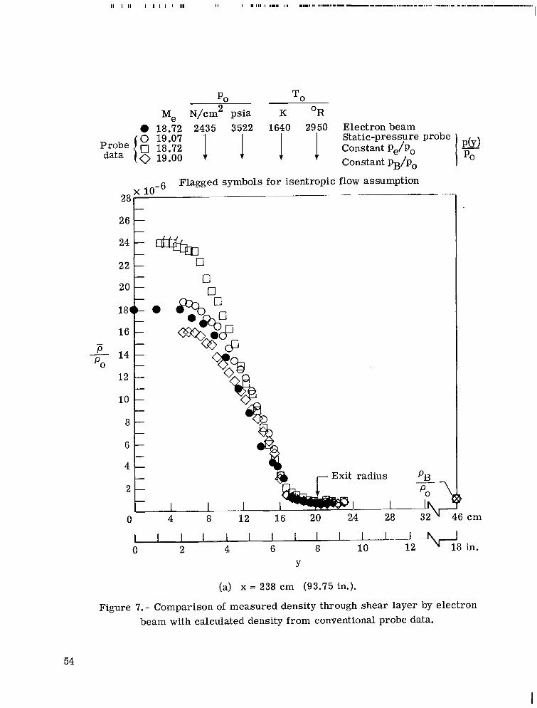
PO TO

Me N/cm 2 psia K OR 0 18.72 2435 3522 1640 2950 Electronbeam

Constant pB/p0

Flagged symbols fo r isentropic flow assumption x .. - ­

26 c

24

0

12

2 Ib

0 6 cm

I -u 0 2 4 6 8 10 --8 in.

Y

(a) x = 238 cm (93.75 in.).

Figure 7. - Comparison of measured density through shear layer by electron beam with calculated density from conventional probe data.

54

P O TO

Me N/cm 2 psia K OR 0 19.76 5460 7910 1722 3010 Electron beam0 20.30 Static-pressure probe

Probe 0 19.58 Constant pe/po p(y>data I 0 20.90 Constant pB/pO PO

x 10-6 Flagged symbols for isentropic flow assumption

I I I I I I I I I I I I

(b) x = 238 cm (93.75 in.); po = 5460 N/cm2.

Figure 7.- Concluded.

55

--

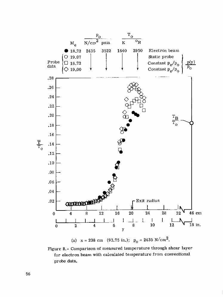
PO TO

Me N/cm 2 psia K OR

18.72 2435 3522 1640 2950

i 1 I 1 .28

.22

.20

.18

.10

.08

.06

.04

.02

0

I I I I _-.A 1 _,I I -_-1~.1. 0 2 4 6 8

Y

Electron beam Static probe constant pe/po Constant pe/po

1 ' w 8 in. 10 12

(a) x = 238 cm (93.75 in.); po = 2435 N/cm2,

Figure 8. - Comparison of measured temperature through shear layer for electron beam with calculated temperature from conventional probe data.

56

PO TO

Me N/cm 2 psia K OR

0 19.76 5460 7910 1722 3010 Electron beam I 0 20.30 I Static press . probe

Probe 0 19.58 Constant pe/po -P(Y)data ] 0 20.90 I l l Constaqt PB/P, PO

.28

-.26

-.24

-.22

-.20 O .

-.18 % .0

-.16 -

-.14 om TO 0

-.12 D

-.10 8 -.08 A

Q

I- Exit radius,I I I \ 7

(b) x = 238 cm (93.75 in.); po = 5460 N/cm2.

Figure 8. - Concluded.

57

PO TO Me N/cm 2 psia K O R

0 18.72 2435 3522 1640 2950 Electronbeam

0 19.07 + J. 4 probe 19.76 5460 7910 1670 3010 Electronbeam

0 20.30 4 + J- 1 probe

Flagged symbols for viscous corrected data.

-

-8 ­ %- 0

0,

2

0 6 cm

Figure 9.- Comparison of static pressure through shear layer from electron-beam profiles with static -pressure probe. x = 238 cm (93.75 in.).

58

----

---

-Re,d x/d Reference Instrumentation

1 -2.60 3.93 X lo4 5.9 21 Static-pressure probe 2 0.938 6.16 + 1.65 21 Static-pressure probe 3 ---- 19.76 1.38 X l o6 0.328 Present Static-pressure probe 4 19.76 + + 0.328 4 Electron beam

1.2

I-\ ' \

1.o /(\\

\ \ 1

2 \ '\ / /---­

.8 \

'\ \ /' - .6 PB Po2

\ II\ )(\ \ Po2

.4 \ \

' \ ' \ \/--

\ I / 1 ', /

// 3 and 4

L' .2 \

\

I 1 dl 1 1 1 0 .2 .4 .6 .8 1.o 1.2 1.4

Y d

Figure 10. - Comparison of measured static pressure ac ross free shear layers at high and low speeds. X with arabic number denotes pB/p, value corresponding to the curves for p/p,.

59

I

PO T O

Data N/cm 2 psia OR K

-0 18.72 2435 3522 1640 2950 ----a19.76 5460 7910 1722 3010

percent

Exit radius I I I

0 4 8 12 1 6 20 24

1 I I I I I I I I I I I 0 2 4 6 8 10 12

Y

Figure 11. - Root -mean-square density fluctuations through shear layer obtained from electron-beam measurements. x = 238 cm (93.75 in.).

60

---- --

6 X cm in. Ref. cm in.

Me R q 6 TW/To Nozzle -8.25-8.89 5.37 to 10.75 x lo4 0.07 to 0.16 13.2-15.0 5.2-5.9 29 wall

18.72 - 2.33 x 105 0.183 17.8 (7.0) Present 238 93.75 19.76 4.60 0.180 15.3 (6.0) + + +

.22

.20 Experiment (ref. 27) (wall boundary layer)

/-\/ \

/ \ / \

\ .12 \

\I \

.08

.04

0 .2 .4 .6 .8 1.0 7/6

Figure 12. - Comparison of intensity of density fluctuations.

61

I

Y PO To cm in. Me ~ / c m ~psia K OR

0 11.41 4.5 18.72 2435 3522 1640 2950 0 12.70 5.0 0 13.99 5.5 1 1 1 1 . 1d 16.50 6.5

17.80 7.0 Af = 50 HZ

I-C -” 0 a, [I]

10-8 I I I I I I LLLL. I 1 I I I L L L L I 1 I 1 I L I L I

1x 10-1 1 1x lo1 1x l o2 f , kHz

(a) R, = 1.3 X 106 per m (Rm= 4.0 X lo5 per ft).

Figure 13. - Energy spectra of density fluctuations for stations ac ross shear layer. x = 238 cm (93.75 in.).

62

V

cm in.

0 11.41 4.5 0 12.70 5.0 0 13.99 5.5 A 15.25 6.0 A 16.50 6.5

17.80 7.0 n 19.05 7.5

PO TO

Me ~ / c m ~psia K OR

1 2 31 LO

Af = 50 HZ

(b) R, = 3.3 X lo6 per m (Rm = 9.2 X 105 per ft).

Figure 13. - Concluded.

6 3

I '

---

Y6 M R-9 x "/"e cm in. Reference

5.0 4.68 x lo6 0.60 1.75 (0.69) 30 ----- 18.72 1.84 x lo5 0.83 17.80 (7.0) Present

19.76 4.21 x lo5 0.78 15.30 (6.0) 4 lo1

loo

I I I I I I I l l I I I I I I l l I I I I I I l l 10-1 loo lo1

Figure 14.- Comparison of power spectra in free shear layers.

64

102

4VOLTMETER

I DENSITY MEASUREMENT SYSTEM

i i I I I

TUNNEL ITEST AREA I

I I

PHOTOMULTIPLIER I

I PHOTOMULTIPLIER

I

ELECTRON I GUN I

I I

1 I

I /I 1 TUNNEL I I

I

I Gain = 1-1000 Gain.27

I

I fiVOLTMETER $-$q 1 ANALOG TAPE I VOLTMETER

DIGITAL h TUNNEL - 1 CONTROL

ROOM Gain =I13

TEMPERATURE MEASUREMENT SYSTEM

PICOAMMETER DIGITAL VOLTMETER

1 &LECTRON-BEAM SYSTEM

ELECTRON PICOAMMETER

ELECTRONICS VOLTMETER

DATA RECORDING srsrE,w

COUPLER

MANUAL

PRINTER

Figure 15. - Electron-beam density and temperature measurement system.

l1 l l11l II I1 Il l I I I I I I I I I I

-Light collection optical axis

Density detection apparatus optical

axis I I Top viewI

. ~- . .- ~ -

Mirror

\

I 1 5 cm

I

ia Mirror /

- 6.4 cm-I Side view

Figure 16. - Density measurement system.

66

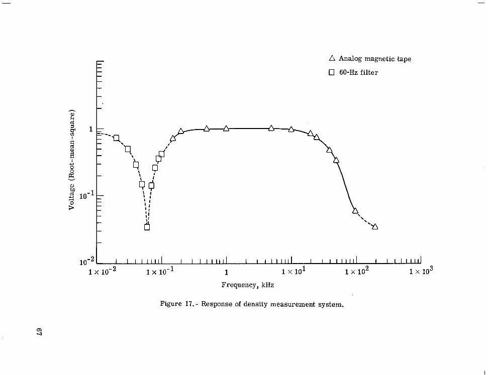
A Analog magnetic tape

0 60-Hz filter

-

I I I I 1 1 1 1 l I I I I I I l l1 I 1 1 I I l l l l I I I I I I I I l I I I I I Ill1

Figure 17. - Response of density measurement system.

manual b

b

Code translator c Instrument

Magnetic

Code c coupler

recorder translator

c

Trigger4-Trigger7

Figure 18. - Data system block diagram.

l-l-l-l-l­

0 0

/ /

- Data fairing

Figure 19. - Temperature calibration curve,

V I

0 Data

Ta = 296 K '(534 OR)

Data fairing (Least squares fit)

Molecular number density

Figure 20. - Density calibration curve.

70 NASA-Langley, 1915 L-10138

NATIONAL AERONAUTICS AND SPACE ADM IN ISTRATION WASHINGTON. D.C. 20546

POSTAGE A N D FEES P A I D N A T I O N A L AERONAUTICS A N D

OFFICIAL BUSINESS SPACE A D M I N I S T R A T I O N PENALTY FOR PRIVATE USE $300 SPECIAL FOURTH-CLASS RATE 451

USMAIL BOOK

8 5 6 001 Cl U D 7 5 0 8 2 2 50090305

O E P T OF THE A I R F O R C E A F k E A P C N S L A B L R A T C R Y A T T N : 1ECHNlCAL L I E P A P Y 1SUL) K I R T L A h G A F E NIY. 87117

: If Undeliverable (Section 158 Postal Rlnnnnl) Do Not Return

__ ­ _ -

'"The aeronautical and space activities of the United States shall be conducted so as t o contribute . . . t o the expansion of human knowl­edge of phenomena in the atmosphere and space. T h e Administration shall provide for the widest practicable and appropriate dissemination of information concerning its activities and the results thereof."

-NATIONAL AERONAUTICSAND SPACEACT OF 1958

NASA SCIENTIFIC AND TECHNICAL PUBLICATIONS TECHNICAL REPORTS: Scientific and technical information considered important, complete, and a lasting contribution to existing knowledge. TECHNICAL NOTES: Information less broad in scope but nevertheless of importance as a contribution to existing knowledge.

TECHNICAL MEMORANDUMS: Information receiving limited distribution because of preliminary data, security classifica­tion, or other reasons. Also includes conference proceedings with either limited or unlimited distribution. -CONTRACTOR REPORTS: Scientific and technical information generated under a NASA contract or grant and considered an h-q"tant contribution to existing knowledge.

TECHNICAL TRANSLATIONS: Information published in a foreign language considered to merit NASA distribution in English.

PUBLICAT1oNS: Information derived from or of value to NASA activities. Publications include final reports of major projects, monographs, data compilations, handbooks, sourcebooks, and special bibliographies.

TECHNOLOGY UTILIZATION PUBLICATIONS: Information on technology used by NASA that may be of particular interest in commercial and other-non-aerospace applications. Publications include Tech Briefs, Technology Utilization Reports and Technology Surveys.

Details on the availability of these publications m a y b e obtained from:

SCIENTIFIC AND TECHNICAL INFORMATION OFFICE

N A T I O N A L A E R O N A U T I C S A N D SPACE A D M I N I S T R A T I O N Washington, D.C. 20546