1  

Experimental Results on Gravity Driven Fully Condensing Flows in Vertical Tubes, their

Agreement with Theory, and their Differences with Shear Driven Flows’ Boundary-

Condition Sensitivities

Jorge Kurita, Michael Kivisalu, Soumya Mitra, Ranjeeth Naik, and Amitabh Narain

Department of Mechanical Engineering-Engineering Mechanics

Michigan Technological University

Houghton, MI 49931

ABSTRACT

This paper synthesizes experimental results reported here with computational results towards development

of a reliable heat transfer correlation for a specific annular condensation flow regime inside a vertical tube. For

fully condensing flows of pure vapor (FC-72) inside a vertical cylindrical tube of 6.6 mm diameter and 0.7 m

length, the experimental measurements are shown to yield values of average heat transfer co-efficient, and

approximate length of full condensation.

The experimental conditions cover: mass flux G over a range of 2.9 kg/m2-s ≤ G ≤ 87.7 kg/m2-s,

temperature difference ∆T (saturation temperature at the inlet pressure minus the mean condensing surface

temperature) of 5 ºC to 45 ºC, and cases for which the length of full condensation xFC is in the range of 0 < xFC <

0.7 m.

The range of flow conditions over which there is good agreement (within 15%) with the theory and its

modeling assumptions has been identified. Additionally, the ranges of flow conditions for which there are

significant discrepancies (between 15 -30% and greater than 30%) with theory have also been identified.

The paper also refers to a brief set of key experimental results with regard to sensitivity of the flow to time-

varying or quasi-steady (i.e. steady in the mean) impositions of pressure at both the inlet and the outlet. The

experimental results support the updated theoretical/computational results that gravity dominated condensing

flows do not allow such elliptic impositions, whereas, shear driven condensing flows (representative

experimental results are also presented) are sensitive to such impositions.

Key Words: Internal Gravity Driven Condensing Flows, Condensation inside Vertical Tubes, Annular

Condensing Flows

2  

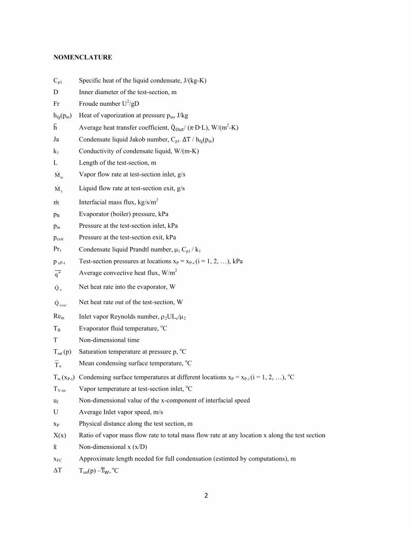
NOMENCLATURE

Cp1 Specific heat of the liquid condensate, J/(kg-K)

D Inner diameter of the test-section, m

Fr Froude number U2/gD

hfg(pin) Heat of vaporization at pressure pin, J/kg

h  Average heat transfer coefficient, QO / (π·D·L), W/(m2-K)

Ja Condensate liquid Jakob number, Cp1· ∆T / hfg(pin)

k1 Conductivity of condensate liquid, W/(m-K)

L Length of the test-section, m

inM Vapor flow rate at test-section inlet, g/s

LM Liquid flow rate at test-section exit, g/s

Interfacial mass flux, kg/s/m2

pB Evaporator (boiler) pressure, kPa

pin Pressure at the test-section inlet, kPa

pexit Pressure at the test-section exit, kPa

Pr1 Condensate liquid Prandtl number, ·Cp1 / k1

p xP-i Test-section pressures at locations xP = xP-i (i = 1, 2, …), kPa

q Average convective heat flux, W/m2

bQ Net heat rate into the evaporator, W

totalQ Net heat rate out of the test-section, W

Rein Inlet vapor Reynolds number, 2ULc/2

TB Evaporator fluid temperature, oC

T Non-dimensional time

Tsat (p) Saturation temperature at pressure p, oC

wT Mean condensing surface temperature, oC

Tw (xP-i) Condensing surface temperatures at different locations xP = xP-i (i = 1, 2, …), oC

TV-in Vapor temperature at test-section inlet, oC

uf Non-dimensional value of the x-component of interfacial speed

U Average Inlet vapor speed, m/s

xP Physical distance along the test section, m

X(x) Ratio of vapor mass flow rate to total mass flow rate at any location x along the test section

x Non-dimensional x (x/D)

xFC Approximate length needed for full condensation (estimted by computations), m

ΔT Tsat(p) –TW, oC

3  

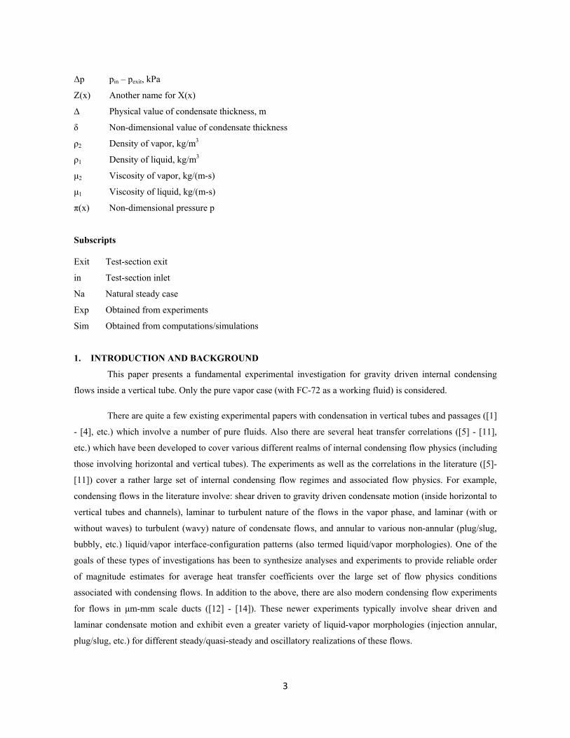
Δp pin – pexit, kPa

Z(x) Another name for X(x)

∆ Physical value of condensate thickness, m

δ Non-dimensional value of condensate thickness

ρ2 Density of vapor, kg/m3

ρ1 Density of liquid, kg/m3

μ2 Viscosity of vapor, kg/(m-s)

μ1 Viscosity of liquid, kg/(m-s)

π(x) Non-dimensional pressure p

Subscripts

Exit Test-section exit

in Test-section inlet

Na Natural steady case

Exp Obtained from experiments

Sim Obtained from computations/simulations

1. INTRODUCTION AND BACKGROUND

This paper presents a fundamental experimental investigation for gravity driven internal condensing

flows inside a vertical tube. Only the pure vapor case (with FC-72 as a working fluid) is considered.

There are quite a few existing experimental papers with condensation in vertical tubes and passages ([1]

- [4], etc.) which involve a number of pure fluids. Also there are several heat transfer correlations ([5] - [11],

etc.) which have been developed to cover various different realms of internal condensing flow physics (including

those involving horizontal and vertical tubes). The experiments as well as the correlations in the literature ([5]-

[11]) cover a rather large set of internal condensing flow regimes and associated flow physics. For example,

condensing flows in the literature involve: shear driven to gravity driven condensate motion (inside horizontal to

vertical tubes and channels), laminar to turbulent nature of the flows in the vapor phase, and laminar (with or

without waves) to turbulent (wavy) nature of condensate flows, and annular to various non-annular (plug/slug,

bubbly, etc.) liquid/vapor interface-configuration patterns (also termed liquid/vapor morphologies). One of the

goals of these types of investigations has been to synthesize analyses and experiments to provide reliable order

of magnitude estimates for average heat transfer coefficients over the large set of flow physics conditions

associated with condensing flows. In addition to the above, there are also modern condensing flow experiments

for flows in μm-mm scale ducts ([12] - [14]). These newer experiments typically involve shear driven and

laminar condensate motion and exhibit even a greater variety of liquid-vapor morphologies (injection annular,

plug/slug, etc.) for different steady/quasi-steady and oscillatory realizations of these flows.

4  

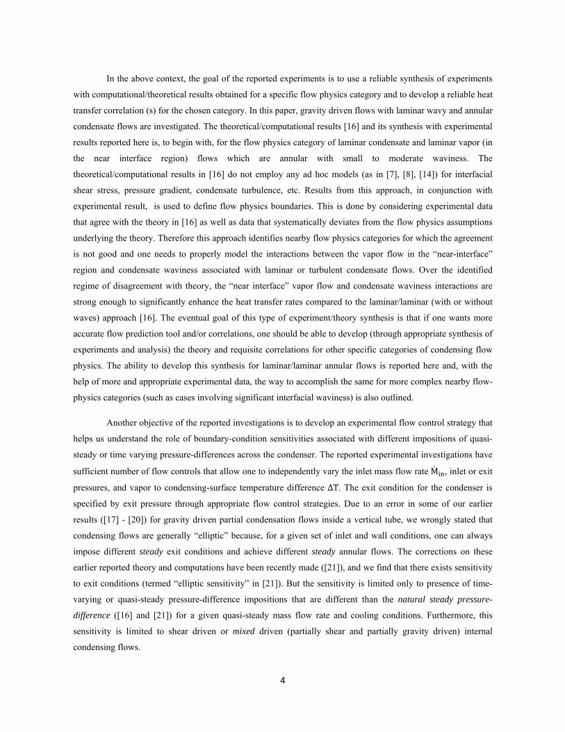
In the above context, the goal of the reported experiments is to use a reliable synthesis of experiments

with computational/theoretical results obtained for a specific flow physics category and to develop a reliable heat

transfer correlation (s) for the chosen category. In this paper, gravity driven flows with laminar wavy and annular

condensate flows are investigated. The theoretical/computational results [16] and its synthesis with experimental

results reported here is, to begin with, for the flow physics category of laminar condensate and laminar vapor (in

the near interface region) flows which are annular with small to moderate waviness. The

theoretical/computational results in [16] do not employ any ad hoc models (as in [7], [8], [14]) for interfacial

shear stress, pressure gradient, condensate turbulence, etc. Results from this approach, in conjunction with

experimental result, is used to define flow physics boundaries. This is done by considering experimental data

that agree with the theory in [16] as well as data that systematically deviates from the flow physics assumptions

underlying the theory. Therefore this approach identifies nearby flow physics categories for which the agreement

is not good and one needs to properly model the interactions between the vapor flow in the “near-interface”

region and condensate waviness associated with laminar or turbulent condensate flows. Over the identified

regime of disagreement with theory, the “near interface” vapor flow and condensate waviness interactions are

strong enough to significantly enhance the heat transfer rates compared to the laminar/laminar (with or without

waves) approach [16]. The eventual goal of this type of experiment/theory synthesis is that if one wants more

accurate flow prediction tool and/or correlations, one should be able to develop (through appropriate synthesis of

experiments and analysis) the theory and requisite correlations for other specific categories of condensing flow

physics. The ability to develop this synthesis for laminar/laminar annular flows is reported here and, with the

help of more and appropriate experimental data, the way to accomplish the same for more complex nearby flow-

physics categories (such as cases involving significant interfacial waviness) is also outlined.

Another objective of the reported investigations is to develop an experimental flow control strategy that

helps us understand the role of boundary-condition sensitivities associated with different impositions of quasi-

steady or time varying pressure-differences across the condenser. The reported experimental investigations have

sufficient number of flow controls that allow one to independently vary the inlet mass flow rate M , inlet or exit

pressures, and vapor to condensing-surface temperature difference ∆T. The exit condition for the condenser is

specified by exit pressure through appropriate flow control strategies. Due to an error in some of our earlier

results ([17] - [20]) for gravity driven partial condensation flows inside a vertical tube, we wrongly stated that

condensing flows are generally “elliptic” because, for a given set of inlet and wall conditions, one can always

impose different steady exit conditions and achieve different steady annular flows. The corrections on these

earlier reported theory and computations have been recently made ([21]), and we find that there exists sensitivity

to exit conditions (termed “elliptic sensitivity” in [21]). But the sensitivity is limited only to presence of time-

varying or quasi-steady pressure-difference impositions that are different than the natural steady pressure-

difference ([16] and [21]) for a given quasi-steady mass flow rate and cooling conditions. Furthermore, this

sensitivity is limited to shear driven or mixed driven (partially shear and partially gravity driven) internal

condensing flows.

5  

The experimental and theoretical results confirming “elliptic-sensitivity” for shear driven flows

(whether they occur in μm-scale ducts or perfectly horizontal channels or zero-gravity duct flows) are reported

separately in [21]. These results are of enormous significance in properly ensuring repeatable realizations of

annular/stratified shear driven flows – which happen to be less repeatable and robust than the gravity driven

flows reported in this paper. The shear driven flows’ elliptic sensitivity results are also important in

understanding the greater variety and complexity of shear driven condensing flows’ liquid/vapor morphologies -

such as those observed in large diameter horizontal tubes (see Carey [22]) and in μm-scale ducts ([12], [14])).

Improper or inadvertent imposition of exit-conditions may also be the cause for various flow transients ([23] -

[25]) observed for “mixed” or purely shear driven internal condensing flows in horizontal tubes. Furthermore, as

theoretically and experimentally shown in [21], availability of suitable time-periodic fluctuations in flow

variables (mass flow rate, inlet/outlet pressures, etc.) is key to enabling multiple pressure-difference impositions

that, independent of any impact on flow rates, affects condensate thickness and leads to different quasi-steady

shear driven annular flows with large changes (> 20 – 30 %) in heat transfer rates.

It is shown here that gravity driven and gravity dominated internal condensing annular flows (see [16]

for the definition of this flow) do not allow externally imposed changes in self-selected exit conditions if inlet

pressure, inlet mass flow rate, and condensing-surface thermal conditions are specified (i.e. the problem is

“parabolic” with no exit-condition sensitivity). Most of the vertical tube cases reported here fall in this gravity

driven and gravity dominated annular internal condensing flow category.

Since this paper deals only with gravity dominated flows and [21] deals only with purely shear driven

flows, we expect that our planned future experiments dealing with mixed driven flows will exhibit elliptic-

sensitivity behavior that is intermediate between these two limiting cases.

2. EXPERIMENTAL APPROACH

2.1 Experimental Facility and Setup

The vertical tube condenser test-section, which is shown in Fig. 1, is a part of a closed flow loop shown

in Fig. 2. The flow loop is designed for investigation of partial and fully condensing flows although fully

condensing flows alone are of interest to this paper. It has three independent feedback control strategies that can

fix and steady the values of: inlet mass flow rate M through active feedback control of the heat input to the

evaporator/boiler, condensing surface temperature TW(x) (uniform or non-uniform) through feedback control of

coolant water flow rate and its temperature, and inlet pressure pin through active feedback control of one of the

controllable displacement pumps in the set up. The flow in Fig. 2 is also especially designed to allow

development of procedures under which condensing flows can be allowed to reach steady state while seeking

their own self-selected exit conditions (exit quality or pressure). These flows with self-selected exit conditions

6  

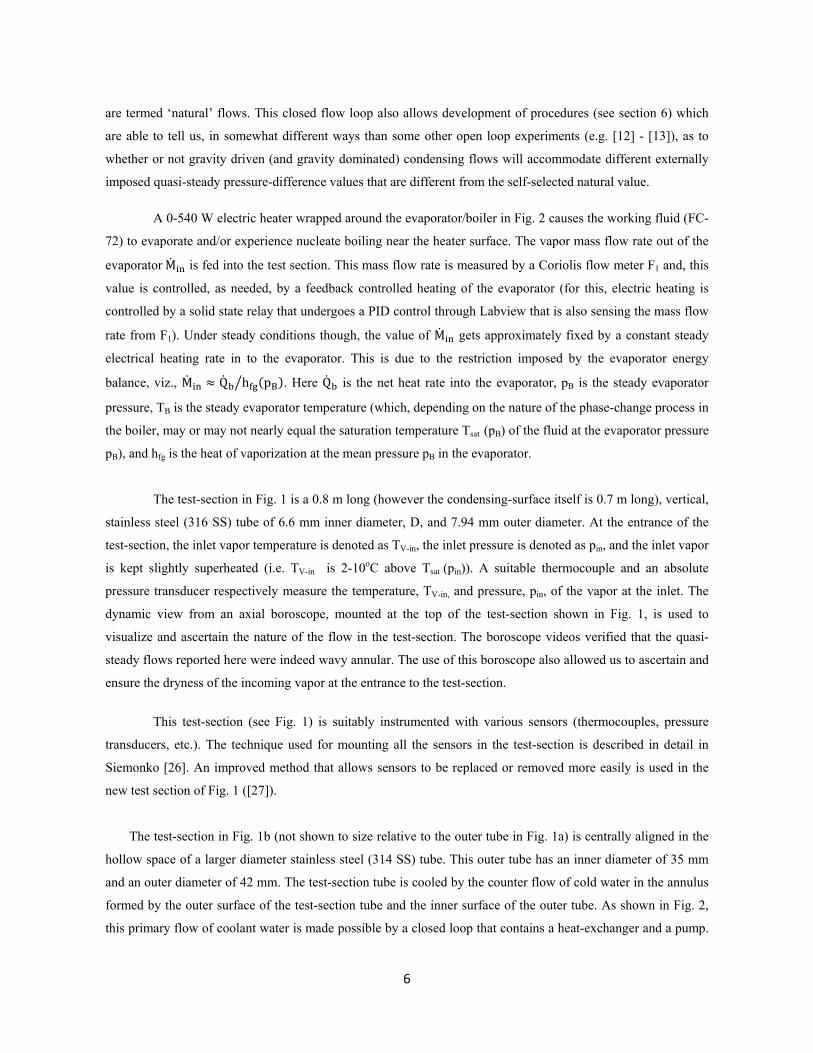
are termed ‘natural’ flows. This closed flow loop also allows development of procedures (see section 6) which

are able to tell us, in somewhat different ways than some other open loop experiments (e.g. [12] - [13]), as to

whether or not gravity driven (and gravity dominated) condensing flows will accommodate different externally

imposed quasi-steady pressure-difference values that are different from the self-selected natural value.

A 0-540 W electric heater wrapped around the evaporator/boiler in Fig. 2 causes the working fluid (FC-

72) to evaporate and/or experience nucleate boiling near the heater surface. The vapor mass flow rate out of the

evaporator M is fed into the test section. This mass flow rate is measured by a Coriolis flow meter F1 and, this

value is controlled, as needed, by a feedback controlled heating of the evaporator (for this, electric heating is

controlled by a solid state relay that undergoes a PID control through Labview that is also sensing the mass flow

rate from F1). Under steady conditions though, the value of M gets approximately fixed by a constant steady

electrical heating rate in to the evaporator. This is due to the restriction imposed by the evaporator energy

balance, viz., M Q h pB . Here Q is the net heat rate into the evaporator, pB is the steady evaporator

pressure, TB is the steady evaporator temperature (which, depending on the nature of the phase-change process in

the boiler, may or may not nearly equal the saturation temperature Tsat (pB) of the fluid at the evaporator pressure

pB), and hfg is the heat of vaporization at the mean pressure pB in the evaporator.

The test-section in Fig. 1 is a 0.8 m long (however the condensing-surface itself is 0.7 m long), vertical,

stainless steel (316 SS) tube of 6.6 mm inner diameter, D, and 7.94 mm outer diameter. At the entrance of the

test-section, the inlet vapor temperature is denoted as TV-in, the inlet pressure is denoted as pin, and the inlet vapor

is kept slightly superheated (i.e. TV-in is 2-10oC above Tsat (pin)). A suitable thermocouple and an absolute

pressure transducer respectively measure the temperature, TV-in, and pressure, pin, of the vapor at the inlet. The

dynamic view from an axial boroscope, mounted at the top of the test-section shown in Fig. 1, is used to

visualize and ascertain the nature of the flow in the test-section. The boroscope videos verified that the quasi-

steady flows reported here were indeed wavy annular. The use of this boroscope also allowed us to ascertain and

ensure the dryness of the incoming vapor at the entrance to the test-section.

This test-section (see Fig. 1) is suitably instrumented with various sensors (thermocouples, pressure

transducers, etc.). The technique used for mounting all the sensors in the test-section is described in detail in

Siemonko [26]. An improved method that allows sensors to be replaced or removed more easily is used in the

new test section of Fig. 1 ([27]).

The test-section in Fig. 1b (not shown to size relative to the outer tube in Fig. 1a) is centrally aligned in the

hollow space of a larger diameter stainless steel (314 SS) tube. This outer tube has an inner diameter of 35 mm

and an outer diameter of 42 mm. The test-section tube is cooled by the counter flow of cold water in the annulus

formed by the outer surface of the test-section tube and the inner surface of the outer tube. As shown in Fig. 2,

this primary flow of coolant water is made possible by a closed loop that contains a heat-exchanger and a pump.

7  

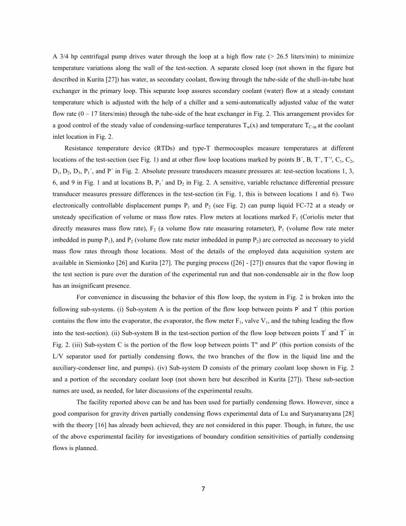
A 3/4 hp centrifugal pump drives water through the loop at a high flow rate (> 26.5 liters/min) to minimize

temperature variations along the wall of the test-section. A separate closed loop (not shown in the figure but

described in Kurita [27]) has water, as secondary coolant, flowing through the tube-side of the shell-in-tube heat

exchanger in the primary loop. This separate loop assures secondary coolant (water) flow at a steady constant

temperature which is adjusted with the help of a chiller and a semi-automatically adjusted value of the water

flow rate (0 – 17 liters/min) through the tube-side of the heat exchanger in Fig. 2. This arrangement provides for

a good control of the steady value of condensing-surface temperatures Tw(x) and temperature TC-in at the coolant

inlet location in Fig. 2.

Resistance temperature device (RTDs) and type-T thermocouples measure temperatures at different

locations of the test-section (see Fig. 1) and at other flow loop locations marked by points B´, B, T´, T´′, C1, C2,

D1, D2, D3, P1´, and P´ in Fig. 2. Absolute pressure transducers measure pressures at: test-section locations 1, 3,

6, and 9 in Fig. 1 and at locations B, P1´ and D2 in Fig. 2. A sensitive, variable reluctance differential pressure

transducer measures pressure differences in the test-section (in Fig. 1, this is between locations 1 and 6). Two

electronically controllable displacement pumps P1 and P2 (see Fig. 2) can pump liquid FC-72 at a steady or

unsteady specification of volume or mass flow rates. Flow meters at locations marked F1 (Coriolis meter that

directly measures mass flow rate), F2 (a volume flow rate measuring rotameter), P1 (volume flow rate meter

imbedded in pump P1), and P2 (volume flow rate meter imbedded in pump P2) are corrected as necessary to yield

mass flow rates through those locations. Most of the details of the employed data acquisition system are

available in Siemionko [26] and Kurita [27]. The purging process ([26] - [27]) ensures that the vapor flowing in

the test section is pure over the duration of the experimental run and that non-condensable air in the flow loop

has an insignificant presence.

For convenience in discussing the behavior of this flow loop, the system in Fig. 2 is broken into the

following sub-systems. (i) Sub-system A is the portion of the flow loop between points P′ and T′ (this portion

contains the flow into the evaporator, the evaporator, the flow meter F1, valve V1, and the tubing leading the flow

into the test-section). (ii) Sub-system B in the test-section portion of the flow loop between points T′ and T′′ in

Fig. 2. (iii) Sub-system C is the portion of the flow loop between points T" and P (this portion consists of the

L/V separator used for partially condensing flows, the two branches of the flow in the liquid line and the

auxiliary-condenser line, and pumps). (iv) Sub-system D consists of the primary coolant loop shown in Fig. 2

and a portion of the secondary coolant loop (not shown here but described in Kurita [27]). These sub-section

names are used, as needed, for later discussions of the experimental results.

The facility reported above can be and has been used for partially condensing flows. However, since a

good comparison for gravity driven partially condensing flows experimental data of Lu and Suryanarayana [28]

with the theory [16] has already been achieved, they are not considered in this paper. Though, in future, the use

of the above experimental facility for investigations of boundary condition sensitivities of partially condensing

flows is planned.

8  

2.2 Operating Procedure

Procedure for “Natural/Unspecified” Exit Condition Cases for Fully Condensing Gravity Driven Flows

To realize fully condensing flows in the flow loop schematic of Fig. 2, the auxiliary condenser flow-

section is removed (valves V3 and V4 are closed). The liquid completely fills the line from some “point of full

condensation” in the test-section all the way to the boiler/evaporator (this means that the liquid fills all the

locations marked as T , L/V separator, and the electronically controllable displacement pump P1). “Natural/self-

selected” fully condensing flow cases is achieved in this set-up by two different procedures.

In procedure-1, the inlet mass flow rate Min is held fixed by the evaporator heater control, the

condensing surface temperature Tw(x) by coolant temperature and flow rate control of the coolant in the

secondary loop, and, inlet vapor temperature TV-in is steadied (at a desired value through an electric heating tape

on the vapor line feeding into the test-section). The inlet pressure is allowed to seek a natural value of pin = pin|Na

as well as the exit pressure is allowed to seek a certain natural value of pexit = pexit|Na by making the exit liquid

mass flow rate ML-e (through the displacement pump P1) track the inlet mass flow rate Min (measured through

Coriolis meter F1) through the tracking equation ML-e|P1= Min. The steady values of the inlet and exit pressures

that are eventually achieved lead to a well defined self-selected “natural” pressure difference Δp|Na = pin|Na –

pexit|Na. The dryness of the vapor at the inlet is ensured through boroscope visualization and a check that the

superheat condition TV-in > Tsat (pin) is satisfied.

The same value of Δp|Na is also achieved by a second (and preferred) procedure, viz. procedure-2. In this

procedure-2, different long term steady values of inlet vapor mass flow rate Min are achieved by active

evaporator heat control while the displacement pump P1 holds fixed the inlet pressure pin = pin* at different set

values. This is possible because the pump P1 is controlled through a Proportional-Integral-Derivative (PID)

controller which, through ups and downs in the flow rate passing through P1 is able to attain a steady pin = pin*

and a steady in the mean flow rate through P1. These mass flow rate shifts through the pump P1 eventually

become minuscule around the steady continuous mass flow rate value of Min through the Coriolis meter F1.

During this operation, inlet temperature TV-in (manipulated through the control of the tape heater on the line

between F1 and the test-section inlet), and the mean wall temperature TW (manipulated through the control of the

secondary coolant’s flow rate and its chiller controlled temperature) are steadied and held fixed at approximate

desirable values. When the flow steadies to some “self selected/natural” steady exit pressure pexit*, a steady value

of Δp = pin*- pexit* = Δp|Na is obtained.

It is found, for the same Min and ΔT, Δp values obtained from procedure- 2 is the same as the one

obtained through procedure-1. The advantage of procedure-2 is that it allows one to change temperature

difference ∆T TS p – TW by changing pressure pin without any need for changing Tw (x) to achieve

different mean temperatures Tw.

9  

2.3 Error Analysis, Repeatability, and Flow Morphology for the Experimental Data

The accuracies of all the instruments (except the Coriolis meter F1) used for reported values of directly

measured variables were established after their in-house calibrations with the help of suitable and reliable

reference instruments of known resolution and appropriate reference physical conditions (temperature, flow rate,

pressure, etc.).

The accuracy of the Coriolis meter was established by the vendor support staff at the time of its

installation. The error estimates for the calculated variables reported in Table 1 were obtained by well-known

standard procedures (see [29]) described in the Appendix. When experimental results are given in a tabular form

(such as Table 1), the accuracies of both measured and calculated variables within a column is taken into

account. For variables whose errors are either due to resolution in the measurement or are significantly lower

order of magnitude than the variables involved, the maximum value of these errors are reported in the headers of

appropriate columns in Table 1. For variables whose errors correlate with the mean values of the variables itself,

percentage relative errors (both mean and maximum values) are reported in the relevant column headers.

In addition to error estimates, repeatability of the fully condensing flows for independent runs were

established for a few randomly selected flow cases. For brevity, this The repeatability is only shown for a set of

fully condensing flows in Figs. 3a - b. Identical results were obtained over three independent time segments

shown in Figs. 3a – b. These repeatable condensing flow results also indicate the repeatable performance and

control of the pumps, cooling systems, temperature controls, etc. that form the various subsystems shown in Fig.

2. Furthermore, procedure - 1 for fully condensing flows (described in section 2.2) was used for achieving the

steady flow in the first time segment of Fig. 3b and procedure - 2 was used for achieving steady flows shown in

the second and third time segments of Fig. 3b. Since Δp values in Fig. 3b are the same for all the three steady

states (which have approximately the same Min and ΔT values), the result experimentally demonstrates the fact

that these gravity driven flows are sufficiently stable [20] and are able to self-seek their own exit conditions (like

“parabolic” flows) in multiple experimental realizations.

The boroscope video mounted on the top of the test-section indicated that all the gravity driven flows

reported and investigated here (see Fig. 4) exhibited an ability to seek and retain robust wavy annular flows.

3. EXPERIMENTAL RESULTS FOR VERTICAL TUBE AND COMPARISONS WITH THEORY

Notations Used for Reporting Experimental Results

Let Ṁ be the inlet mass flow rate of the vapor, and ∆T be a fixed representative value of a certain

vapor to wall temperature difference profile. Let ṀL x and ṀV x be the condensate and the vapor mass flow

rates at any given location x (0 ≤ x ≤ L) along the test section length. Let the inlet Reynolds number be given as

Rein ≡ ρ2UD/µ2 where U is the average speed of vapor at the inlet (i.e.

10  

Ṁ π4 D ρ U ). Here 2 and 2 are, respectively, representative constant values of vapor density and

viscosity. Note that all vapor properties are assumed to be approximately uniform and their representative

constant values are evaluated at the pressure of pin (the test-section inlet pressure) and a temperature of 1oC

superheat over the saturation temperature associated with pin. Thus the Reynolds number represents a specific

non-dimensional form of Ṁ . The non dimensional temperature difference ∆T is expressed as the ratio of

condensate Jacob Number (Ja Cp . ∆T h⁄ ) to the condensate Prandtl Number (Pr µ . Cp k⁄ ) i.e.

Ja Pr ∆T. µ h . k⁄⁄ . Here 1, 1, k1, and Cp1 are, respectively, representative constant values of liquid

density, viscosity, thermal conductivity, and specific heat. All liquid properties are evaluated at the pressure of

pin and a temperature of “ TW 0.5 · ∆T.” Also hfg ≈ hfg(pin) is the heat of vaporization at a representative

pressure that is close to the mean condenser pressure for the reported experimental runs. The gravity vector is

expressed in terms of the components gx - along the test section and gy - in the transverse direction, where their

non dimensional values are Frx-1 = gx.D/U2 and Fry

-1 = gy.D/U2. Since gy = 0 for a vertical tube, Fry-1 = 0. For

convenience, we have replaced Frx-1 by a new non dimensional gravity parameter GP Fr . Re

ρ . g D µ⁄ which is independent of the inlet flow rate. Therefore the non-dimensional parameter set that

impacts and characterizes the vertical in-tube condenser flow is: {x/D, Rein, GP, Ja/Pr1, ρ2/ρ1, µ2/µ1}.

Because, for most reported data, the counter flow of cooling water surrounding the test-section is at a

fixed flow rate (8 gallons/min) and at nearly fixed temperatures (20-30°C – sufficient to ensure that water

properties do not change significantly), the condensing-surface temperature variations TW(x) is adequately

modeled by the assumption of a uniform surface temperature TW. This is because for any two representative

experimentally measured wall temperature variations TW1(x) and TW2(x) shown in Fig. 5a, it is found that the

variation of non-dimensional condensing-surface temperature θW x ( TW x TW ∆T⁄ ) with non-

dimensional distance x x/D is nearly the same function (within experimental errors) for all cases. This means

that, in the non-dimensional formulation of the problem ([16]), the thermal condition for the condensing-surface

remains the same. Furthermore we verified that the simulation results (based on the methods described in [16])

were nearly the same, with regard to the overall quantities of interest to this paper, for a non-uniform

temperature TW(x) and for the associated uniform temperatureTW. The non-monotonous trend of θW x in Fig.

5a is understandable and its x variations associated with varying flow physics of increasing thickness of a nearly

smooth condensate, onset of significant waviness, and eventual single phase nature of the flow.  

Experimental Range and Results

The experimental results given in Table 1 for the fully condensing flows show key details of different

and representative flow runs. These results were obtained by the flow loop arrangement in Fig. 2 and the

procedures 1 and 2 described in section 2.2. The experimental runs reported in Table 1 cover only a portion of

the non-dimensional parameter space {x, Rein, Gp ((ρ22gx Dh

3) / μ22), Ja/Pr1, ρ2/ ρ1, μ2/μ1} that governs this in-

tube problem. With distance x from the inlet satisfying the constraints FC0 x x for full condensation cases

11  

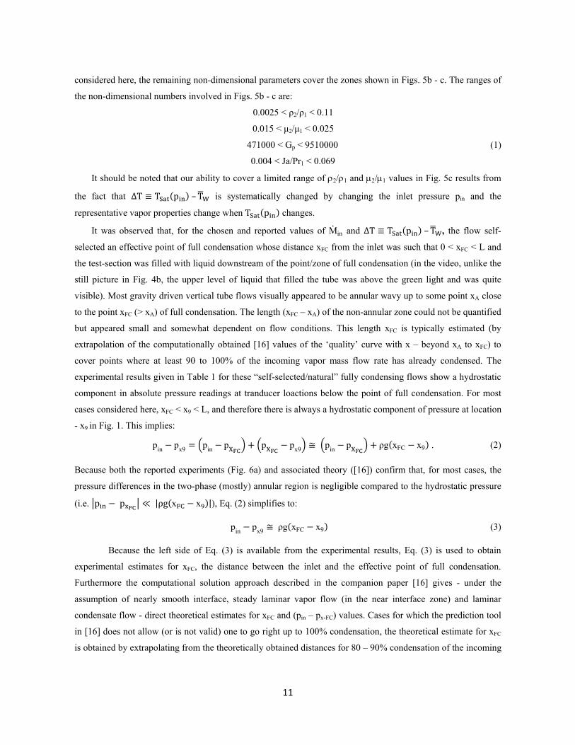
considered here, the remaining non-dimensional parameters cover the zones shown in Figs. 5b - c. The ranges of

the non-dimensional numbers involved in Figs. 5b - c are:

0.0025 < ρ2/ρ1 < 0.11

0.015 < μ2/μ1 < 0.025

471000 < Gp < 9510000 (1)

0.004 < Ja/Pr1 < 0.069

It should be noted that our ability to cover a limited range of 2/1 and 2/1 values in Fig. 5c results from

the fact that ∆T TS p – TW is systematically changed by changing the inlet pressure pin and the

representative vapor properties change when TS p changes.

It was observed that, for the chosen and reported values of Min and ∆T TS p – TW, the flow self-

selected an effective point of full condensation whose distance xFC from the inlet was such that 0 < xFC < L and

the test-section was filled with liquid downstream of the point/zone of full condensation (in the video, unlike the

still picture in Fig. 4b, the upper level of liquid that filled the tube was above the green light and was quite

visible). Most gravity driven vertical tube flows visually appeared to be annular wavy up to some point xA close

to the point xFC (> xA) of full condensation. The length (xFC – xA) of the non-annular zone could not be quantified

but appeared small and somewhat dependent on flow conditions. This length xFC is typically estimated (by

extrapolation of the computationally obtained [16] values of the ‘quality’ curve with x – beyond xA to xFC) to

cover points where at least 90 to 100% of the incoming vapor mass flow rate has already condensed. The

experimental results given in Table 1 for these “self-selected/natural” fully condensing flows show a hydrostatic

component in absolute pressure readings at tranducer loactions below the point of full condensation. For most

cases considered here, xFC < x9 < L, and therefore there is always a hydrostatic component of pressure at location

- x9 in Fig. 1. This implies:

pin px9 pin pXFCpXFC

px9 pin pXFCρg xFC x9 . (2)

Because both the reported experiments (Fig. 6a) and associated theory ([16]) confirm that, for most cases, the

pressure differences in the two-phase (mostly) annular region is negligible compared to the hydrostatic pressure

(i.e. p pFC

|ρg xFC x |), Eq. (2) simplifies to:

pin px9 ρg xFC x9 (3)

Because the left side of Eq. (3) is available from the experimental results, Eq. (3) is used to obtain

experimental estimates for xFC, the distance between the inlet and the effective point of full condensation.

Furthermore the computational solution approach described in the companion paper [16] gives - under the

assumption of nearly smooth interface, steady laminar vapor flow (in the near interface zone) and laminar

condensate flow - direct theoretical estimates for xFC and (pin – px-FC) values. Cases for which the prediction tool

in [16] does not allow (or is not valid) one to go right up to 100% condensation, the theoretical estimate for xFC

is obtained by extrapolating from the theoretically obtained distances for 80 – 90% condensation of the incoming

12  

vapor. Although predictions of |(pin – px-FC)| is off, its order of magnitude is correct and, therefore it is found that

the right side of Eq. (3) correctly approximates the right side of Eq. (2).

For fully condensing flows, the experimental value of the average heat-transfer coefficient h (or hE ) is

obtained from Eq. (4) below. For this, the experimental estimates of Min, xFC, and ∆T TS p – TW are used

in Eq. (4).

Qout≈ Minhfg = (πD·xFC · h )∆T (4)

The theoretical value of the average heat-transfer coefficient h (or hS ) is obtained by employing the

computationally obtained values for the distance xFC in Eq. (4). The resulting value of hS is found to be

equivalent ([16]), or nearly the same, as the one obtained from the relationship:

h FC

·∆

· dxFC  

          

                                                                      (5) 

where the film thickness ∆ x D · δ x   and the expression on the right of Eq. (5) is evaluated by the

computational solution approach described in [16].

As shown in Figs. 6b-c, whenever the laminar vapor/laminar condensate assumption is adequate, there

is an excellent agreement (within 3 - 4%) between theoretical and experimental estimates of xFC. Equivalently,

because of Eq. (3) we also have an agreement between experimental and theoretical estimates of ∆p ≡ (px9 - pin).

In Figs. 6b-c, the reported plots show the functional dependence structure of xFC = xFC (Min, ∆T) as one of the

two variables (Min or ∆T) is varied while the other is held fixed. Figures 6b-6c show the cases for which the

experimentally calculated xFC starts becoming significantly smaller than the theoretically calculated xFC at larger

values of M and ∆T. Therefore, Figs. 6b-6c, provide us with a good opportunity to experimentally obtain and

develop a quantitative criteria as to when the near interface region of the vapor flow starts interacting strongly

with laminar waviness or turbulence of the condensate in the near interface region. A reasonable procedure for

quantifications of these effects, that appear to be the most probable cause (given the videos show the annularity

of these flows) for theory and experiment to deviate from one another, is described in section 4.

The full condensation runs/cases associated Figs. 5b-c also allows a comparison of theoretically and

experimentally obtained values of the average heat-transfer coefficient h. These comparisons are shown in Fig.

6d.

13  

4. EFFECTS OF INTERACTIONS BETWEEN NEAR-INTERFACE VAPOR FLOW AND

CONDENSATE FLOWS’ INTERFACIAL WAVINESS

4.1 Observed Deviations Between Experimental and Theoretical Results

As seen in Figs. 7a-7b, there are significant numbers of experimental data points for fully condensing

flows where the experimentally measured values of the heat transfer coefficients are significantly more than the

idealized theoretical estimates. For convenience of analysis, we have sorted the data points based on their

deviation from the idealized theory and defined the measure as: Deviation E T

E100. The sorting in

Fig. 7a is done in “Ja/Pr1 - Rein” plane and in Fig. 7b in “Ja/Pr1 - Re | FC

4ML FC

πDµ1” plane. A pictorial

depiction of this sorting, as shown in Figs. 7a-7b, is in the following three groups: (i) experimental values of h

that are within 15% (represented by filled diamond points), (ii) experimental values of h that are between 15% -

30% above the correlated or theoretical values (represented by hollow diamond points), and (iii) experimental

values of h that are more than 30% above the correlated or theoretical values (represented by the filled circular

points). These experimentally obtained data are also the same for which, in Figs. 6a-6b, the indirectly measured

experimental values of xFC are smaller than the predicted values of xFC. The fact that the experimental heat

transfer rate is higher and the point of full condensation is smaller is understandable. Near the inlet, despite

turbulence of the vapor in the core regions, the condensate is thin, laminar, and nearly smooth (except for

vibration induced waves). The large value of interfacial mass-flux and associated large bending of vapor stream

lines at small distances from the inlet (see, e.g., stream line patterns in [20]) makes the “near interface” vapor

flow zone laminar despite turbulence in the core regions. However, for these gravity driven condensate flows,

the condensate accelerates and by a certain downstream distance, the laminar condensate motion develops

significant instability induced (different from wall noise induced) interfacial waves and, further downstream, the

condensate flow becomes turbulent - as is the also the case for the gravity driven Nusselt problem ([5] and [30]).

At such downstream distances, despite laminarization of the slowing vapor in the core regions, the near interface

vapor flow regions can become turbulent due to the accelerating condensate flow becoming turbulent at x

locations where Reδ x4ML

πDμ1 is sufficiently large. Note that [30] suggests that the order of magnitude of Reδ

values where gravity driven laminar condensate becomes wavy is 30 to 100 and where it becomes turbulent is

500 to 1000.

The curves C1 (and C2) in Fig. 7a suggests that the critical inlet Reynolds number - which determines

whether or not near-interface laminarity or turbulence of the vapor is possible over the length of interest (0 ≤ x ≤

xFC) - also depends on the temperature-difference parameter Ja/Pr1 which is known to control the interfacial

mass transfer rates (see Eq. (6) in [16]). Similarly curves C1′ (and C2

′) in Fig. 7b suggests that the critical

condensate Reynolds number Re | FC

4ML FC

πDµ1

4Min

πDµ1 - which determines at what distance x relative to xFC

the laminar condensate becomes significantly wavy and/or significantly turbulent – also depends on the average

14  

interfacial mass transfer rate modeled by the parameter Ja/Pr1. This dependence of critical values of Rein or

Reδ|x xFC on interface mass transfer rate (as modeled by Ja/Pr1) is expected because vapor lines bend and pierce

the interface (see, e.g., [19]) with significant reduction in the x- component of the vapor speed in the near

interface region. The extent of reduction in the x-component of vapor speed by the time vapor reaches the

interface also depends on the value of Reδ x - a measure of the increasing inertia of the condensate.

By reprocessing the results in Figs. 7a-7b in terms of the parameters used for the x-axes in Figs. 8a-8b, we

arrive at the following results for FC-72 flows’ annular condensation inside vertical tubes:

I. The effects of near-interface vapor turbulence and near-interface condensate waviness are small (in the

sense that the laminar/laminar smooth-interface model [16] for these flows are adequate) provided

Re 60000Ja

Pr

.

and Re | FC700

J

P

. (6)

II. The effects of near-interface vapor turbulence and near-interface condensate waviness enhance the

average heat transfer coefficient h by a factor between 1.15 and 1.3 provided

60000Ja

Pr1

0.

Rein 88000Ja

Pr1

0.

and 700J

P

.Re | FC

1250J

P

. (7)

III. The effects of near-interface vapor turbulence and near-interface condensate waviness enhance the

average heat transfer coefficient h by a factor greater than 1.3 provided

Re 88000Ja

Pr

.

and Re | FC1250

J

P

. (8)

4.2 Reasons for Deviations and Suggested Modeling for Wavy and Turbulent Annular Flows

Based on the above results, it is likely that, as and when one has access to experimentally measured

“local” values of heat transfer coefficient hx, or heat flux q x , then one could use – in conjunction with the

existing steady [16] and a full unsteady simulation capability being developed by our group (as in [21]) - a local

interfacial vapor Reynolds number ReVL(x) to characterize local transition from smooth interface steady

laminar/laminar conditions to significant interfacial waviness without turbulence as well as significant waviness

with turbulence. This number is defined here as ReVL x ρ Uu x /τ where, as in [16], Uu x and i

are, respectively, time-averaged mean of the physical values of interfacial speed and shear stress. Because the

condensate continues to speed up under gravity, the same number ReVL(x) can also be used to characterize

15  

subsequent transition to near-interface vapor/liquid turbulence. This parameter ReVL(x) is also the reciprocal of

the much sought after interfacial friction factor f x τ /ρ Uu x whose non-dimensional definitions as

well as models vary in the literature (see [15]).

From the one-dimensional smooth-interface laminar/laminar theory presented in the companion paper

[16], we know that the flow is predictable in terms of three variables viz., non-dimensional interfacial speed

uf(x), non-dimensional film thickness (x), and non-dimensional pressure gradient d(x)/dx. This is done in [16]

with the help of an appropriate approximate model for friction factor f and, concurrently, a model for the vapor

momentum flux (with the interfacial shear from the vapor profile preferably matching the value from the

interfacial shear model) through their known explicit functional dependence on the non-dimensional variables:

uf(x), (x), and d(x)/dx. The approximate explicit analytical model for f(x) in the 1-D approach [16] is easily

obtained from using the thin film, laminar/laminar flow, and negligible inertia assumptions leading to condensate

profile given by Eq. (7) of [16]. Utilizing this profile and setting i (≡ 2U2· uf

2(x)·f(x)) equal to its value in terms

of interfacial velocity gradient i ≡ 1U/D·∂u1/∂y|i, one obtains an explicit model for f(x) ≡ 1/ReV(x). The

resulting explicit model/relationship for the friction factor f(x) is:

2 1 2 1f f 1 2 x in 2 1

2

2u (x) f (x) u (x) d (x) / dx / Fr Re (x) 1 / 2 /

(x)

. This functional

dependence for f(x) exhibits the general dependence on the three x-dependent non-dimensional flow variables of

uf(x), (x), and d/dx (x) along with dependence on the non-dimensional constant parameters: 2/1, 2/1, Rein,

and Fr-1x. This formulation as well as the model for f(x) ≡ 1/ ReVL(x) can also be equivalently obtained in terms

of three other suitable variables, such as: non-dimensional interfacial speed uf(x), non-dimensional film thickness

(x), and non-dimensional local condensate Reynolds number Re x 4ML x /πDµ (where ṀL x is the

physical value of the local condensate mass flow rate).

For the gravity dominated flow runs (as defined in [16]) that are experimentally considered in Figs. 6 –

7 above, the condensate motion is approximately characterized by the Nusselt solution [5] for a range of inlet

flow rates and one can either use the 1-D theory in [16] or use the single degenerate ordinary differential

equation in (x) (given in [5]) to obtain the Nusselt solution that yields (x) as well as uf(x) and Re(x). In this

degenerate gravity dominated limit, vapor momentum balance is completely independent of the condensate

motion (and need not be solved if the interest is in the condensate motion alone) and vapor mass balance yields

the variations in the average value of the vapor speed. This degeneracy for gravity dominated flows arise from

the fact that interfacial shear i or uf2(x)·f(x) is nearly zero relative to wall shear. Yet one can use the full 1-D

solution scheme [16] to obtain the still negligible values of uf2(x)·f(x) up to a certain x = x* and this is done and

resulting values of a gradually increasing ReVL(x) = 1/f(x) is schematically (i.e. not to scale) shown in Fig. 9.

However, downstream of a certain x = x*, finite amplitude instability induced waves develop ( [16], [30]). In the

zone x > x*, interfacial shear i or uf2(x)·f(x) is significantly non-zero and should not be ignored. The value of x*

itself can be obtained by more detailed experiments or by the unsteady computational approaches described in

[19] - [21]. Once x* is obtained, one can still use the full 1-D solution scheme [16] to obtain the still negligible

16  

values of uf2(x*)·f(x*). If one has to match the negligible shear behavior for x ≈ x* to the wave-induced non-

negligible shear behavior for x > x*, one must discard the Nusselt model for the condensate velocity profile and

use the one given by Eq. (7) in [16]. For x > x*, one can set uf2(x)·f(x) = w(x) ·uf

2(x*)·f(x*) where w(x) > 1 is an

empirically/computationally knowable function of x that can be determined to model the wave-enhanced

interfacial shear so as to make the predicted mean values of the flow variables (such as mean film thickness and

wall heat-flux) agree with their experimentally measured values for x > x*. Finding “w(x)” or “f(x)” this way

will be far superior to ad hoc modeling of interfacial shear ([15]).

The knowledge of uf2(x)·f(x) from 1-D theory [16] for x < x* along with its modification uf

2(x)·f(x) =

w(x)·uf2(x*)·f(x*) for x > x* , can be used to express the pressure gradient d (x)/dx as a function of uf(x) and

(x) (or Re(x)) for x > x*. This suggested modification of the 1-D scheme for x > x* would only allow two

unknown independent variables (say uf(x) and (x) or uf(x) and Re(x)) in the modeling and solution for x > x*.

This is a natural outcome of using an empirically obtained function w(x) to replace one of the unknowns (say d

(x)/dx ) for x > x*. The suggested formulation and solution (not done here) of the problem for x > x* in terms of

the two chosen variables (say uf(x) and Re(x)) can be used to show that, as x approaches x* in Fig. 9, the value

of ReVL (x) approaches a certain critical constant value of ReVL|Cr-1.

The trends of ReVL(x), Re(x), Rein(x), in Fig. 9 for x < x* is for a specific gravity dominated flow

situation and is representative (though not to scale) of the trends obtained by the solution scheme described in

[16]. The trends in Fig. 9 for the laminar/laminar wavy zone over x* ≤ x ≤ x** and the turbulent/turbulent wavy

zone for x ≥ x** are entirely schematic and need to be obtained with the help of sufficient experimental input

and the modeling approach suggested in the previous paragraph. In Fig. 9, the suggested trend of the parameter

ReVL (x) for x < x* denotes nearly smooth interface steady laminar/laminar conditions, ReVL(x) > ReVL|Cr-1 for x

> x* denotes significant laminar/laminar waviness in the near interface zone, and ReVL(x) > ReVL|Cr-2 for x > x**

denotes significant turbulent/turbulent waviness in the near interface zone. The above suggested developments

for gravity dominated flows will also yield proper models for the interfacial shear i (or f) and would make the

existing models and one dimensional analyses much more reliable outside the currently available [16]

laminar/laminar smooth interface zone.

With the above understanding of ReVL(x), we see that the parameter zone characterized by Eq. (6)

above is one for which the ratio x*/xFC dominates the ratio (xFC - x*)/xFC, the parameter zone characterized by

Eq. (7) above is one for which the ratios (xFC - x*)/xFC and x*/xFC are comparable in magnitude, and the

parameter zone characterized by Eq. (8) above is one for which the ratio (xFC - x*)/xFC starts dominating the

ratio x*/xFC.

It is reiterated that the above described synthesis of theory with experiments require experimental data

on distances where transition to waviness and turbulence occur, mean local values of heat-flux in the wavy and

turbulent condensate zone, etc. for different working fluids. As and when such a synthesis is achieved, one

should be able to replace the numerical multipliers and exponents appearing in Eqs. (6) – (8) by multipliers and

exponents that are functions of GP, ρ2/ρ1, and µ2/µ1. Such a generalization of Eqs. (6) – (8), along with heat

17  

transfer co-efficient values obtained from a one dimensional theory (see [16]), will yield more reliable estimates

of vertical in-tube condensation heat-transfer coefficients (for different working fluids) in the wavy and turbulent

regimes.

5. REMARKS ON COMPARISONS WITH WELL KNOWN CORRELATIONS AND

RECOMMENDATIONS

As seen from the theory ([16], [21]) and notations defined in section - 3, the non-dimensional numbers

that affect these condensing flows can be represented by the set {x x/D, Rein, GP, Fry1, Ja/Pr1, ρ2/ρ1, µ2/µ1}.

Well known experimental correlations ([5] - [10], etc.), including those listed in Table 2, often replace the

parameter set { x x/D , Rein, Ja/Pr1} by {Reδ(x), Rein, X(x)} where the condensate’s film Reynolds number is

Reδ x 4ML x /πDμ1 and the local vapor quality is X x Z x MV x /Min. As a result of the above

choices, one finds that most of the existing correlations ([4] - [11], etc.), directly or indirectly use the non-

dimensional parameter set: {X(x), Reδ(x), Rein, GP, ρ2/ρ1, µ2/µ1}. One significant drawback of this choice of

parameters is that even when a heat transfer correlation provides a reasonable order of magnitude estimate, the

correlation itself is not useful for estimating the length of a condenser for a given heat load unless the correlation

is supplemented by experimentally measured or analytically/computationally obtained (as is the case here) axial

variation in quantities such as X(x), Reδ(x), etc. This drawback is not present for the explicit correlations

(involving x) presented in this and the companion paper [16] for annular wavy gravity driven flows.

In actual practice, for a given fluid, the fluid parameter ρ2/ρ1 and µ2/µ1 do not affect the flow as much as

the other parameters. Of these remaining parameters, the set {Rein, GP, Reδ} have a profound impact on the flow

physics in the sense that together they determine: (i) certain well defined low to high ranges of Rein for which

the core vapor flow is turbulent over a significant length of the flow and it affects the pressure-difference across

the two-phase region, (ii) certain well defined low, high, and intermediate ranges of values for GP (see [16])

decides whether the flow is shear driven, gravity driven, or driven by a combination of shear and gravitational

forces, and (iii) certain well defined low to high ranges of Reδ (also discussed in Eqs. (6) - (8)) determine

whether or not the near-interface region of the condensate flow exhibits sufficient waviness (with or without

turbulence).

The above discussion suggests that the parameters {Rein, GP, Reδ} in the header of Table 2 determine,

loosely speaking, at least eight distinct pairs of permutations of these three parameters (e.g. {high, low, low})

that define different flow physics groups - each of which require separate experimental and modeling attention.

Of these, for purely shear driven flows, one typically does not need to consider high Reδ cases involving

condensate turbulence as the condensate flows’ Reδ is seldom as high as those for gravity driven flows (which

may, see [30], high Reδ in the range of 500-1000).

As seen in Table 2, the popular correlations in the literature ([4] - [11], etc.) are developed over multiple

flow physics groups because they attempt an ambitious synthesis of experimental data obtained for flows in

vertical tubes, horizontal tubes, and horizontal to inclined channels. Even when an attempt is made (as in [11]) to

18  

classify and propose different correlations for different flow regimes (annular, stratified, plug/slug, etc.), the

correlations for annular flow rely heavily on horizontal tube data. Now horizontal tube annular flows require

shear forces to dominate the effects of azimuthal component of gravity vector which requires relatively large

Rein values (see JG > 2.5 criteria in [11]) in an altogether different {Rein, GP} space as compared to vertical in-

tube annular wavy flows considered here. Unlike high Rein and low Gp three dimensional flows in the

correlations given in [11], the flows considered here involve low Rein and high Gp values that allow two-

dimensional annular flows. As a result of the aforementioned reasons, even where the agreement between the

experimentally obtained heat transfer coefficients in this paper and those obtained from related theoretical

correlations [16] are found to be good, the values obtained from other correlations of Shah [6], Cavallini [7] and

[11], Dobson-Chato [8], etc. are not as good (see Fig. 10). The existing correlations can, at best, only provide an

order of magnitude estimate of the average heat transfer coefficient. If higher accuracy correlations need to be

developed, one must seek correlations for the specific physics based subgroups.

As an example, the experiments and analysis [16] are synthesized here to propose correlations that limit

themselves (see the first row of Table 2) to a clear and sharp categorization of the boundaries among shear,

gravity and mixed flow regimes within laminar vapor (low Rein) and laminar condensate (low Reδ) flow regimes.

Furthermore, as discussed in section-4, this paper also makes some contribution, through our experimental

results, to define the boundary of this annular wavy flow regime where an assumption of smallness of wave

effects and near-interface “laminarity” of the vapor and the condensate flows can be considered to be adequate.

In Figs. 7a-7b, most of the experimental data, that agree well (i.e. within 15%) with the theoretical

model in [16], are found to correspond to gravity dominated flows for which either the Nusselt correlations [5]

for high GP or “near” Nusselt correlations for moderate to high GP are adequate. As a result, for the data in the

range specified by Eq. (1), the following correlations can be used:

qw′′ x hx∆T (9)

Nux hxD/ 1 1/δ (10)

where, if GP is large and in the gravity dominated zone defined in [16], we have

Nux 4Ja

Pr1

x

GP

/, (11)

and, if GP is in the moderate to large GP zone defined in [16], we have

Nu. . J P⁄ . ⁄ .

R . µ µ⁄ . (12)

For reasons discussed above, unlike the Shah [6], Cavallini [7], Cavallini [11], Dobson-Chato [8], etc

correlations in Fig. 10, the specialized correlations given in Eqs. (9) - (12) – and restricted by Eqs. (1) and (6) -

are superior for this specific gravity driven annular wavy flow regime (also see Table 2).

19  

6. EXPERIMENTAL RESULTS ON DIFFERENCES BETWEEN GRAVITY AND SHEAR DRIVEN

FLOWS’ BOUNDARY CONDITION SENSITIVITIES

6.1 Background for Boundary-Condition Sensitivity Results

New and careful theoretical and computational investigations ([16], [21]) show that purely shear driven

flows exhibit a certain elliptic-sensitivity to unsteady impositions. Elliptic-sensitivity of condensing flows means

that different independent impositions of pressures with suitable time variations (whether they are steady in the

mean or not) is possible at the inlet and the exit while all other conditions (mass flow rate, condensing-surface

thermal boundary condition associated with the cooling approach, etc.) remain quasi-steady at the same mean

values. For purely shear driven quasi-steady flows, elliptic-sensitivity has been demonstrated (see [21]) for the

case of unsteady or steady-in-the-mean pressure-difference impositions (through concurrent control of inlet and

exit pressures). As a result of this sensitivity, the flow realizations (including heat transfer rates and condensing-

surface temperatures) significantly change in response to different quasi-steady pressure-difference impositions.

This paper reports and summarizes our experimental finding that similar elliptic sensitivity does not exist for

gravity dominated flows. That is, ‘non-natural’ elliptic pressure-difference impositions (different from self-

selected, or “natural” pressure-difference) for the same inlet mass flow rate and coolant flow conditions could

not be imposed for experimental realizations of gravity dominated flows in closed loop systems considered here.

Whenever such non-natural pressure-difference is experimentally imposed on a vertical tube condenser, unlike

the shear driven case in [21], the flow variables within the test-section do not make direct adjustments but they

do so only because the other mechanical boundary condition (namely the quasi-steady mass flow rate) also

changes.

For the gravity dominated in-tube vertical annular flows considered here (see definition of gravity

dominated in [16]), the condensate motion and the associated film thickness (interface location) is completely

determined by gravity as they must follow the Nusselt solution [5]. This makes the coupling between liquid

motion and vapor motion uni-directional in the sense that the liquid motion dictates and achieves the kind of

vapor motion that must be there in order to achieve the Nusselt [5] type behavior for the condensate motion.

Under these conditions, computational simulations (of the type reported in [21]) also fail to show that imposition

of different quasi-steady exit pressure conditions is possible if the inlet conditions (i.e. mass flow rate M and

pressure pin at the inlet of the test section in Fig. 11) as well as the condensing-surface cooling approach are kept

steady/quasi-steady.

In the next two sub-sections, we describe the experimental procedure and results for boundary condition

sensitivity of gravity dominated flows.

20  

6.2 Procedure for Imposition of “Non-Natural” Pressure-difference for Vertical In-tube Flows

For describing the experimental approach needed to assess the elliptic-sensitivity effect for fully

condensing gravity driven flows, the flow loop in Fig. 2 has been slightly modified, and this version is

schematically shown in Fig. 11. This set up is similar to the one used for shear driven flows [21], except that, for

the reported experimental results, the evaporator does not have the water bath within which the evaporator in

Fig. 11 is immersed. The test-section in Fig. 11 is the vertical tube test-section in Fig. 1. In addition, there is an

option to use a controllable compressor between the evaporator and the inlet of the test-section. Since the

compressor is in a bypass loop, if the mass flow rate M is fixed, the degree to which the compressor

contributes energy and adjusts the mean value and fluctuation content of the inlet pressure pin of the vapor as it

enters the test-section is adjusted by the control of the compressor’s rotational speed (rpm) and through the level

of opening/closing of the valve VBP in Fig. 11.

First the self-sought “natural” pressure-difference for fully condensing flows is achieved using a

variation of the procedure described in section 2.2. That is, for these fully condensing cases, the valve V in Fig.

11 is closed and the pump P2 in Fig. 11 is removed and eventually attained steady operating values of M , pin,

and ∆T T p – TW are such that the point of full condensation is within the test-section and the “Collection

Chamber” in Fig. 11 is filled with liquid. The first few steps for the procedure involve: (i) holding fixed the

Coriolis mass flow meter FC reading of the mass flow rate M by manually adjusting and fixing the electrical

power supplied to the evaporator heating element, (ii) fixing the inlet pressure pin = pin* with the help of the PID

control of the rpm of the compressor, and (iii) arriving at one well defined steady condensing surface

temperature TW (x) = TW(x)|Na through control on the primary coolant (water that flows along the outside surface

of the internal refrigerant tube in the test section) flow rate and its temperature. (iv) The “natural” exit pressure

pexit = pexit|Na is achieved (and sensed) by using the controllable displacement pump P1 to merely “track” the

liquid pumping rate through it and set it equal to Coriolis meter mass flow rate M . (v) Then a new PID control

is implemented on the pumping rate of pump P1, using feedback from the pressure sensor which measures pexit ,

to maintain the same exit pressure (pexit|C-1 = pexit|Na). (vi) Afterwards, attempts are made to change the set point

in the pump P1’s PID control, to achieve various different “non-natural” (≠ pexit|Na) values of exit pressure pexit

(pexit|C-2, pexit|C-3, etc.) while holding the inlet pressure at pin = pin*. It is expected that, if quasi-steady non-natural

pressure-difference impositions associated with exit pressure specifications pexit|C-2, pexit|C-3, etc. are possible,

eventually different quasi-steady states should be reached for the fixed heater adjusted steady value of vapor

mass flow rate M (at the Coriolis-meter F1).

21  

6.3 The Inability to Impose Quasi-steady “Non-natural” Pressure-Differences at a Fixed Quasi-steady

Mass Flow Rate for Gravity Dominated Flows.

In the time duration t1 to t1+ 20 min (see Figs. 12-13), the test section boundary conditions were

constrained as indicated above such that the total test section pressure drop for case C-1 is in the vicinity of a

“natural” case for the indicated mass flow rate M , inlet pressure pin, and wall temperature condition TW.

Although the Na-1 case itself is not shown in Figs. 12 and 13, many such natural cases have been obtained

(including all of the experimental cases for the vertical tube condenser used in Figs. 5 - 6) where it was observed,

for representative cases, that long term quasi-steady flow in the test-section is achieved along with a long term

quasi-steady flow in the rest of the system. Therefore, although the time duration for case C-1 (t1 ≤ t ≤ t1+20

min) shown in Figs. 12 - 13 is not long enough to assure long term system steadiness outside of the test-section,

based on our previous experience, it is expected that test-section (pin|C-1, TW|C-1, M |C-1, etc.) and other system

flow variables would remain quasi-steady at their depicted values.

Between time t1+20 min and time t2, the exit pressure (pexit) boundary condition was shifted upward

from pexit|C-1 to pexit|C-2 (see Fig. 12) by changing the set point on the pump P1’s PID control, which resulted in a

temporary slowing down of the liquid pumping rate to allow the level of the liquid in the test section to rise,

thereby reducing the length of full condensation (not shown). Due to such an imposition, the inlet pressure (pin)

would normally rise to compensate for the adjustment and regain a natural pT (≡Δp); however, the compressor

control on pin prevented this from happening (see Figs. 12-13). Instead, between time t1+20 min and time t2, the

compressor PID control reduced the speed of the compressor, C, relieving pressure at the inlet to keep it at the

quasi-steady value of pin shown in Fig. 12.

Case C-2, from time t2 to time t2* appears to have achieved a non-natural quasi-steady value of pT|C-2 ≠

pT|Na-1 flow with other test section variables showing little to negligible shift in their mean values (note small

shift down in wall temperature). However, unlike the case C-1 and Na-1, the flow outside of the test-section did

not achieve any steady-state and this is shown (in Fig. 13) by the unsteady compressor speed C|C-2 and the

evaporator pressure pevap|C-2 over this time duration. An outcome of this unsteadiness is that, at time t2*, pevap|C-2

has shifted upward (see Fig. 12) enough that the evaporation thermodynamics inside the evaporator has changed

to prevent the evaporator from continuing to supply the mass flow rate of M |C-2 ≈ M |C-1; therefore, M |C-2*

reduces between time t2* and time t2**. During this time period, the values of pin and pexit are held fixed in the

mean at pin and pexit|C-2, respectively, by the compressor and the liquid pump P1. Note from Fig. 13 that C|C-2* is

still going down between times t2* and t2**, but not as quickly as C|C-2 between times t2 and t2*. Also note that

pevap|C-2* is still unsteady from time t2* to time t2**, although in the mean it is increasing more slowly than pevap|C-

2 between time t2 and time t2*. In addition, TW|C-2* changes to achieve a new steady value (nearly equal to TW|C-1

at time t2**) consistent with a changed new value of M |C-2** . Some time at or beyond time t2**, the condensing

flow in the test section would achieve a new natural case, case N-2 (not shown in Figs. 12 - 13) for which both

the test-section and the system flow variables will be steady.

22  

The key observation and difference from the shear driven case’s elliptic-sensitivity [21] is that it was

not possible to have Min|C-2** ≈ Min|C-1 (at time t2**) despite the evaporator heater’s attempt to do so. In other

words, the condensing flow did not readjust to accommodate a different Δp for the same M .

From the example reported above and additional experimentation (not reported here for brevity), the

flow loop’s response as to which mechanical boundary condition variables are shifted (mass flow rate M , inlet

pressure pin, etc.) and which could be held fixed depended on the procedure used and relative strengths of

different portions of the flow loop external to the test-section.

An intermediate response for “mixed” driven flows (see definition of “mixed” driven flow in [16]) is

expected and will be demonstrated by us when we redo the experiments in [21] for slightly inclined channels.

The results presented here and in [16] and [21] correct some of our misunderstandings from [17]-[18] in

which a non-existent control for fixing inlet pressure - combined with a non-functional sensing of the inlet

pressure - caused us to erroneously confirm the incorrect conclusion (based on an earlier CFD code result which

has since been corrected in [16] and [21]) that steady gravity dominated flows also exhibited elliptic-sensitivity.

7. CONCLUSIONS

The results presented in this paper achieved the following:

Steady gravity driven condensing flows of pure FC-72 considered here were experimentally realized

for gravity dominated situations and were found to lead to robust annular/stratified flows.

The paper establishes a range of conditions for which the flow is adequately modeled (within 15%) by

the laminar vapor/laminar condensate smooth-interface theory and associated correlations obtained in

the companion paper [16].

The paper described an approach that allowed demarcation of the flow zones where near-interface

vapor turbulence and near-interface condensate waviness interact to significantly enhance the heat

transfer rates and reduce the length of full condensation as compared to the theory in the companion

paper [16].

The paper recommends that higher accuracy heat transfer correlations, if desired, must be obtained by

analysis and experiments that are specialized for a particular flow physics category of internal

condensing flows (eight broad categories have been identified).

The experimental results on boundary-condition sensitivity show that pure shear driven flows are

parabolic with “elliptic-sensitivity” whereas gravity dominated flows are strictly “parabolic”.

ACKNOWLEDGEMENT:

Parts of this research were supported by NASA grants NNC04GB52G and NNX10AJ59G and parts through NSF

grant NSF-CBET-1033591. The experimental results for vertical tube are taken from the Ph.D thesis of J.Kurita.

23  

REFERENCES

[1] J.H. Goodykoontz, R.G. Dorsch, Local heat transfer coefficients for condensation of steam vertical

down flow within a 5/8-inch diameter tube, NASA TN D-3326, 1966.

[2] J.H. Goodykoontz, R.G. Dorsch, Local heat transfer coefficients and static pressures for condensation

of high-velocity steam within a tube, NASA TN D-3953, 1967.

[3] F.G. Carpenter, Heat transfer and pressure drop for condensing pure vapors inside vertical tubes at high

vapor velocities, Ph. D Thesis, University of Delaware, 1948.

[4] A. Cavallini, R. Zechchin, High velocity condensation of R-11 vapors inside vertical tubes, Heat

Transfer in Refrigeration (1971) pp. 385-396.

[5] W. Nusselt, Die Oberflächenkondesation des Wasserdampfes, Zeitschrift des Vereines Deutscher Ing.

60 (27) (1916) pp. 541-546.

[6] M.M. Shah, A General Correlation for Heat Transfer during Film Condensation inside Pipes, Int. J. of

Heat and Mass Transfer 22 (1979) pp. 547-556.

[7] A. Cavallini, J.R. Smith, R. Zechchin, A Dimensionless Correlation for Heat Transfer in Forced

Convection Condensation, 6th Int. Heat Transfer Conference, Tokyo, Japan, 1974.

[8] M.K. Dobson, J.C. Chato, Condensation in Smooth Horizontal Tubes, ASME J. of Heat Transfer (1998)

pp. 193-213.

[9] M. Soliman, J.R. Schuster, P.J. Berenson, A General Heat Transfer Correlation for Annular Flow

Condensation, ASME J. of Heat Transfer (1968) pp. 267-276.

[10] N.Z. Azer, L.V. Abis, T.B. Swearinger, Local Heat Transfer Coefficients during Forced Convection

Condensation inside Horizontal Tubes, Trans. ASHRAE 77 (1977) pp. 182-201.

[11] A. Cavallini, G. Gensi, D. Del Col, L. Doretti, G. A. Longo, L. Rossetto, C. Zilio, Condensation Inside

and Outside Smooth and Enhanced Tubes – A Review of Recent Research, International Journal of

Refrigeration 26 (2003) pp. 373-392.

[12] H.Y. Wu, P. Cheng, Condensation Flow Patterns in Microchannels, Int. J. Heat and Mass Transfer 48

(2005) pp. 286-297.

[13] X.J. Quan, P. Cheng, H.Y. Wu, Transition from Annular to Plug/Slug Flow in Condensation in a

Microchannel, Int. J. Heat and Mass Transfer 51 (2008) pp. 707-716.

[14] J.W. Coleman, S. Garimella, Two-phase Flow Regimes in Round, Square, and Rectangular Tubes

during Condensation of Refrigerant R134a, Int. J. Refrig. 26 (2003) pp. 117-128.

[15] A. Narain, G. Yu, Q. Liu, Interfacial Shear Models and Their Required Asymptotic Form for Annular

Film Condensation Flows in Inclined Channels and Vertical Pipes, Int. J. of Heat and Mass Transfer 40

(1997) pp. 3559 – 3575.

[16] S. Mitra, A. Narain, R. Naik, S.D. Kulkarni, Quasi One-dimensional Theory for Shear and Gravity

Driven Condensing Flows and their Agreement with Two-dimensional Theory and Selected

Experiments, submitted for publication in the Int. J. of Heat and Mass Transfer, 2011.

24  

[17] A. Narain, S. D. Kulkarni, S. Mitra, J. H. Kurita, M. Kivisalu, Internal Condensing Flows in Terrestrial

and Micro-Gravity Environments - Computational and Ground Based Experimental Investigations of

the Effects of Specified and Unspecified (Free) Conditions at Exit, Interdisciplinary Transport

Phenomenon, Annals of New York Academy of Sciences 1161 (2009) pp. 321-360.

[18] A. Narain, J. H. Kurita, M. Kivisalu, S. D. Kulkarni, A. Siemionko, T. W. Ng, N. Kim, L. Phan,

Internal Condensing Flows Inside a Vertical Pipe – Experimental/Computational Investigations of the

Effects of Specified and Unspecified (Free) Conditions at Exit, ASME Journal of Heat Transfer (2007)

pp. 1352-1372.

[19] A. Narain, Q. Liang, G. Yu, X. Wang, Direct Computational Simulations for Internal Condensing

Flows and Results on Attainability/Stability of Steady Solutions, Their Intrinsic Waviness, and Their

Noise-Sensitivity, Journal of Applied Mechanics 71 (2004) pp. 69-88.

[20] L. Phan, X. Wang, A. Narain, Exit Condition, Gravity, and Surface-Tension Effects on Stability and

Noise-sensitivity Issues for Steady Condensing Flows inside Tubes and Channels, International Journal

of Heat and Mass Transfer 49 Issues 13-14 (2006) pp. 2058-2076.

[21] S.D. Kulkarni, A. Narain, S. Mitra, M. Kivisalu, M. M. Hasan, Exit-Condition Sensitivity for Shear and

Gravity Driven Annular/Stratified Internal Condensing Flows. Accepted for publication in the

International Journal of Transport Processes, 2010.

[22] V.P. Carey, Liquid-Vapor Phase-Change Phenomena, Series in Chemical and Mechanical Engineering,

Hemisphere Publishing Corporation, 1992.

[23] G.L. Wedekind, B.L. Bhatt, An Experimental and Theoretical Investigation in to Thermally Governed

Transient Flow Surges in Two-Phase Condensing Flow, ASME Journal of Heat Transfer 99 (4) (1977)

pp.561-567.

[24] B.L. Bhatt, G. L.Wedekind, Transient and Frequency Characteristics of Two-Phase Condensing Flows:

With and Without Compressibility, ASME Journal of Heat Transfer 102 (3) (1980) pp. 495-500.

[25] B.L. Bhatt, G.L.Wedekind, A Self Sustained Oscillatory Flow Phenomenon in Two-Phase Condensing

Flow Systems, ASME Journal of Heat Transfer 102 (4) (1980b) pp. 695-700.

[26] A. Siemonko, Design, Fabrication, and Operation of a System to Control FC-72 Condensation Inside a

Vertical Tube, Ph.D Thesis, Michigan Technological University, 2006.

[27] J.H. Kurita, Experimental investigation of fully condensing downward vapor flows in a vertical tube -

unspecified (free) exit condition cases, Masters Thesis, Michigan Technological University, 2007.

[28] Q. Lu, N. V. Suryanarayana, Condensation of a vapor flowing inside a horizontal rectangular duct,

Journal of Heat Transfer 117 (1995), pp. 418-424.

[29] P. Holman, Experimental Methods for Engineers, sixth edition, McGraw Hill, 1994.

[30] Incropera, F. P. and D. P. Dewitt, Fundamentals of Heat and Mass Transfer, Sixth Edition, Wiley,

2006.

25  

APPENDIX

The reported error calculations involve three kinds of variables, namely: (i) measured variables xMi (i = 1 to N0),

(ii) handbook variables xHi (i = 1 to N1) that report values of various fluid properties, and (iii) calculated

variables xCi (i = 1 to N2) that depend on other (measured, handbook, or calculated) variables. For the directly

measured variables in Tables 1 to 2, we have N0 = 6 with {xM1 ≡ Min, xM2 ≡ pin, xM3 ≡ Tw, xM4 ≡ pexit = px9, xM5 ≡

D, xM6 ≡ L}. The errors xMi have been calculated by in house calibration experiments and/or values

reconfirmed by the vendor of the instrument involved. These error values are: {xM1 = ± 0.05 g/s, xM2 = ± 0.15

kPa, xM3 = ± 0.9oC, xM4 = ± 0.27 kPa, xM5 ≡ ± 0.5 mm, xM6 ≡ ± 0.001 m}. For the handbook variables in

Tables 1 to 2, we have N1 = 7 with {xH1 ≡ 1, xH2 ≡ 2, xH3 ≡ 1, xH4 ≡ Cp1, xH5 ≡ k1, xH6 ≡ hfg (pref), xH7 ≡ Tsat

(pref)}. For these variables, a nominal experimental error of 2% is assumed. That is the error xHi = ± 0.02*xHi

(i = 1 to M1). For the calculated variables (some of them are reported in Table 1), we have N2 = 13 with { xC1 ≡

Tsat (pin|measured), xC2 ≡ hfg (pin), xC3 ≡ T, xC4 ≡ p, xC5 ≡ 2/1, xC6 ≡ 2/1, xC7 ≡ G, xC8 ≡ Re, xC9 ≡ Ja/Pr1, xC10 ≡

Qout, xC11 ≡ h|Expt, xC12 ≡ q , xC13 ≡ xFC|Expt}. For all these calculated variables xCi, the defining equations are

such that they can be reassembled to express their dependence only on the measured and handbook variables. As

a result, one can express the dependences and errors for xCi (assuming a random Gaussian variation in errors) as

per the well known (Holman [29]) expressions:

xCi = fi (xM1, xM2, …, xMN0, xH1, xH2, ….., xHN1) (A.1)

and

xCi =

2 2N0 N1i i

Mi HiMi Hii 1 i 1

f fx x

x x

, (A.2)

where, i = 1 to N2, and each function fi is known as a single explicit function or a function given by a set of

nested explicit functions. Because of these explicit forms of fi, (unlike situations where fi itself is approximately

known with some statistical uncertainty), their derivatives and their values in Eq. (A.2) are easily calculated for

each xCi for any given run in Table 1.

26  

TABLE CAPTIONS

Table 1: Representative experimentally measured data and some key calculated and computed variables

for natural fully condensing steady flows.

Table 2: Representative coverage of the parameter space under different well known empirical or semi-

empirical correlations.

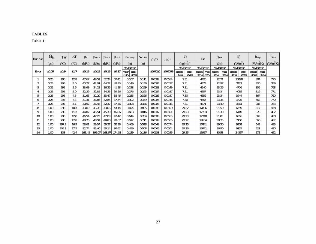
27  

TABLES

Table 1:

(g/s) (°C) (°C) (kPa) (kPa) (kPa) (kPa) (m) (W/m2K)

mean ±11%

max   ±27%

mean   ±34%

max      ±36%

mean  ±21%

max   ±25%

mean   ±13%

max    ±20%

mean   ±22%

max     ±37%

mean  ±25%

max    ±34%

1 0.25 296 12.8 47.67 49.52 52.24 57.41 0.111 0.0039 0.0164 775

2 0.25 296 9.0 40.77 42.01 44.72 49.83 0.159 0.0033 0.0157 769

3 0.25 295 5.6 33.69 34.23 36.25 41.28 0.259 0.0028 0.0149 768

4 0.25 295 5.0 32.29 32.82 34.25 39.26 0.293 0.0027 0.0147 771

5 0.25 295 4.5 31.65 32.20 33.47 38.46 0.326 0.0026 0.0147 760

6 0.25 295 4.3 31.31 31.86 32.85 37.84 0.339 0.0026 0.0146 770

7 0.25 295 4.1 30.92 31.48 32.37 37.36 0.356 0.0026 0.0146 783

8 1.00 296 10.3 43.09 43.78 43.66 43.14 0.895 0.0035 0.0160 478

9 1.00 296 11.2 44.82 45.51 45.39 45.06 0.816 0.0037 0.0161 482

10 1.00 296 12.0 46.54 47.23 47.09 47.42 0.764 0.0038 0.0163 480

11 1.00 296 12.8 48.26 48.94 48.80 49.67 0.711 0.0039 0.0165 482

12 1.00 297.2 16.9 58.61 59.34 59.27 62.38 0.528 0.0048 0.0174 483

13 1.00 306.1 17.5 82.74 83.40 59.14 86.62 0.508 0.0066 0.0204 480

14 1.00 303 42.4 165.48 166.07 168.67 174.33 0.186 0.0138 0.0246 492

hSimpxP-6 pxP-9 xFC-Sim ρ 2/ρ1 μ2/μ1

±0.15 ±0.27 ±0.0010 ±0.0009

pxP-3

Error ±0.05 ±0.9 ±1.7 ±0.15 ±0.15

ΔT pinRun No

0.159

xFC-Exp

0.308

0.694

0.683

0.644

0.612

0.149

0.238

0.276

0.285

0.302

(m)% Error

0.469

0.459

0.107

% Error% Error% Error% Error

29.25 543

(J/s)

q'' hExp

(W/m2K)(W/m2)(kg/m2s)% Error

9203

10278

7423

4706

4085

521

804

820

29.23

29.22 17684

836

8197.31

29.25

ReG

17441

16971

4426

4479

4540

4557

4559

4563

4571

17836

7.30

7.30

7.31

29.22

29.23

29.26

7.31

7.31

7.31

17793

17740

15967

89.50

86.90

22.71

22.97

23.26

23.34

23.34

23.36

23.40

91.50

91.30

91.03

90.75

80.53 24397

569

560

575

867

862

903

617

576

3944

3725

3661

6359

6449

6816

7150

9125

inM wT outQinM wT outQ

28  

Table 2:  

FIGURE CAPTIONS

Fig. 1: (a) The photograph of condenser test-section. (b) The test-section schematic (diameters in (a) and

(b) are not to the same scale). The condensing surface covers the zone x0 ≤ x ≤ x10.

Fig. 2: The schematic of the flow loop for achieving unspecified exit condition flows for partial or full

condensation cases. For full condensation cases, valve V3 is closed and the auxiliary condenser is not in

use.

Fig. 3a: These time histories of inlet mass flow rate, inlet saturation temperature, and average wall

temperature are nearly the same for three separate steady realizations over three separate time intervals.

They are termed unspecified (“natural”) exit condition cases - namely Natural-1, Natural-2, and Natural-

3.

Fig. 3b: Time histories of pin, pexit, and Δp for the three unspecified pressure-difference runs shown in Fig.

3a. The first time-segment’s steady flow realization was by procedure-1 and the steady realizations in the

second and the third time segments were by procedure-2. Though pin in the first segment is different, the

High Low High Low High

Very Low    Moderately 

LowGP Reδ Reδ Rein Rein

Proposals based on this 

paper

Cavallini[1974]

Shah [1979]

Dobson & Chato[1998]

Azer et.al [971]

Travis et.al [1973]

Soliman et.al [1968]

Cavallini [2003]

Correlations Low GP

29  

natural pressure-difference ∆p values are seen to be equal for all the three runs because Min and ∆

– values are approximately the same for all the three cases.

Fig. 4: The light reflected from the interface depicts typical wavy annular flows realized in vertical tube

experiments. The borescope views are taken from the top of the test-section and the blue/green lights are

vertically down at a location below the test-section. The blue light picture on the left is for a representative

partial condensation case and the green light picture on the right is for a representative full condensation

case.

Fig. 5a: The figure shows two different condensing-surface temperature variations TW1(x) and TW2(x)

corresponding to runs 12 and 13 in Table 1. It also shows corresponding non-dimensional temperatures

with repect to non-dimensional = x/D.

Fig. 5b: The investigated full and partial condensation flow cases cover the parameter space {Rein, Gp,

Ja/Pr1} above.

Fig. 5c: The investigated full and partial condensation flow cases cover the parameter space {ρ2/ ρ1, μ2/μ1}

space above.

Fig. 6a: For a representative case (run 14 in Table 1), the plot shows test-sectional pressure variation with

distance x. The measurements are at locations x0, x3, x6, and x9 marked in Fig. 1. The value of xFC is

marked to indicate its estimated value.

Fig. 6b: The comparison of theoretically and computationally obtained values of xFC as a function of Min.

Here the the dashed lines indicates the simulation results and the solid lines indicate the experimental

results.

Fig. 6c: The comparison of theoretically and computationally obtained values of xFC as a function of T.

Here the the dashed lines indicates the simulation results and the solid lines indicate the experimental

results.

Fig. 6d: Comparison of experimentally and computationally obtained values of average heat transfer

coefficients for fully condensing flows.

30  

Fig. 7a: The plot shows deviation levels (between theory and experiments) with respect to the variables

Ja/Pr1 (representing ΔT) and the inlet Reynolds number Rein (representing ). The solid black diamond

points show less than 15% deviation from the idealized theory. The hollow diamond points show

experimental heat transfer coefficient values higher by 15% - 30% and hollow circular points show that

the experimental heat transfer values were greater than 30% with respect to the idealized theoretical

estimates.

Fig. 7b: The plot shows deviation levels (between theory and experiments) with respect to the variables

Ja/Pr1 (representing ΔT) against the condensate film’s Reynolds number Reδ at x = xFC. The solid black

diamond points show less than 15% deviation from the idealized theory. The hollow diamond points show

experimental heat transfer coefficient values higher by 15% - 30% and hollow circular points show that

the experimental heat transfer values were greater than 30% with respect to the idealized theoretical

estimates.

Fig. 8a: Plot of deviation against inlet parameter Rein/(Ja/Pr1)0.2718. The solid black diamond points show

less than 15% deviation from the idealized theory. The hollow diamond points show experimental heat

transfer coefficient values higher by 15% - 30% and the hollow circular points show that the experimental

heat transfer values were greater than 30% with respect to the idealized theoretical estimates.

Fig. 8b: Plot of discrepancy against inlet parameter | / / . at x= xFC. The solid black

diamond points show less than 15% deviation from the idealized theory. The hollow diamond points show

experimental heat transfer coefficient values higher by 15% - 30% and the hollow circular points show

that the experimental heat transfer values were greater than 30% with respect to the idealized theoretical

estimates.

Fig. 9: For modeling heat transfer enhancement greater than 15%, the figure shows the schematic of

variations, with distance x, for the near interface vapor turbulence parameter ReVL(x), vapor flow

Reynolds number ReV(x), and the condensate Reynolds number Re(x).

Fig. 10: The figure shows a comparison of experimentally obtained heat transfer coefficient with heat

transfer coefficients obtained from evaluating different correlations with the help of our simulation tool’s

predictions [16]. The figure limits itself to assessing the efficacy of various correlations for the gravity

dominated flows considered here.

Fig. 11. Flow loop arrangement for investigation of various boundary-condition sensitivities of internal

partially or fully condensing flows (gravity or shear driven).

31  

Fig. 12. Representative experimental time histories for test-section and flow-loop pressures demonstrating

inability of gravity driven internal condensing flows to achieve steady state (at a fixed inlet mass flow rate)

under imposition of “non-natural” pressure-difference values.

Fig. 13. Representative experimental time histories for test-section and flow-loop temperatures, inlet flow

rate, and compressor speed demonstrating inability of gravity driven internal condensing flows to achieve

steady state (at a fixed inlet mass flow rate) under imposition of “non-natural” pressure-difference values.

This data corresponds to the same periods of time over which the data in Fig. 12 were obtained.

c

32  

FIGURES

Fig. 1

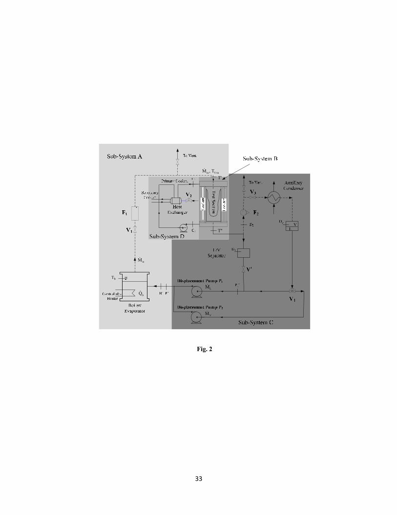
33  

 

 

 

LM

inM

bQ

in V-inM , T

T'

T''

bT

VM

Fig. 2

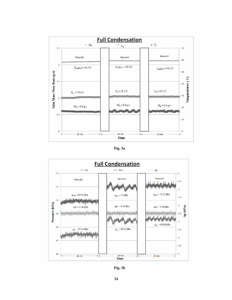
34  

Fig. 3a

Fig. 3b

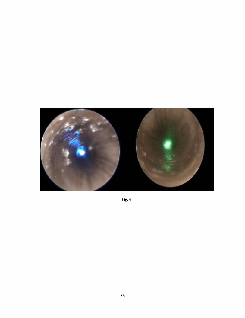
35  

Fig. 4

36  

Fig. 5a

Fig. 5b

0 5 10 15 20 25 30 35 40 45 50 55 60 65 70 75

‐0.20

‐0.15

‐0.10

‐0.05

0.00

0.05

0.10

0.15

0.20

0.25

0.30

20

22

24

26

28

30

32

34

36

38

40

0 0.05 0.1 0.15 0.2 0.25 0.3 0.35 0.4 0.45

Non‐Dimensional Distance [x/D]

Non

‐Dim

ension

al Wall Tem

perature, w (x/D

)

Physical Wall Tem

perature, Tw(x) (de

gree

s C)

Physical Distance, x (m)

Case‐1: Tw1(x): Physical

Case‐2: Tw2(x): Physical

Case‐1:  ‐w(x/D) : Non‐Dimensional

Case‐2:  ‐w(x/D) : Non‐Dimensional

Run‐12: {Min =1.00 g/s, TW|1 =24.1°C, T1 =16.9°C, pin|1 =58.6 kPa, Tc,in|1 =20.4°C}Run‐13: {Min =1.00 g/s, TW|2 =32.9°C, T2 =17.5°C, pin|2 =82.7 kPa, Tc,in|2 =29.5°C}

Case‐1

Case‐2

Case‐1

Case‐2

37  

Fig. 5c

0.015

0.017

0.019

0.021

0.023

0.025

0.027

0.000 0.002 0.004 0.006 0.008 0.010 0.012 0.014 0.016 0.018 0.020

2/

1

2/1

38  

Fig. 6a

Fig. 6b

165

166

167

168

169

170

171

172

173

174

175

0 0.1 0.2 0.3 0.4 0.5 0.6 0.7

Absolute Pressure (kPa)

Distance from Test Section Inlet (m)

Test Section Pressure Profile

Test Section Pressures

Hydrostatic Gradient

xFC‐Expx6

x9x0 x3

Modeled TwoPhase Pressure

0.00

0.10

0.20

0.30

0.40

0.50

0.60

0.70

0.80

0.90

1.00

1.10

0.0000 0.0005 0.0010 0.0015 0.0020 0.0025 0.0030 0.0035

Mass Flow Rate (kg/s)

41.4 kPa Exp.

41.4 kPa Sim

55.2 kPal Exp.

55.2 kPa Sim

72.1 kPa Exp.

72.1 kPa Sim

117.2 kPa Exp.

117.2 kPa Sim

168.5 kPa Exp.

168.5 kPa Sim

172.5 kPa Exp.

172.5 kPa Sim

39  

Fig. 6c

Fig. 6d

0.000

0.100

0.200

0.300

0.400

0.500

0.600

0.700

0.800

0.900

1.000

1.100

1.200

0.0 4.0 8.0 12.0 16.0 20.0 24.0 28.0 32.0 36.0 40.0 44.0

Length of Full Con

densation 

xfc(m

)

Test Section T (K)

0.25 g/s Min Exp

0.25 g/s Min Sim

1.00 g/s Min Exp

1.00 g/s Min Sim

1.00 g/s Min (Higher Twall) Exp

1.00 g/s Min (Higher Twall) Sim

1.75 g/s Min Exp

1.75 g/s Min Sim

2.00 g/s Min Exp

2.00 g/s Min Sim

0

100

200

300

400

500

600

700

800

900

1000

0 100 200 300 400 500 600 700 800 900 1000

Theo

retical H

eat Transfer C

oefficient (W

/m2 K)

Experimental Heat Transfer Coefficient (W/m2K)

Dev <15%

Dev < 30%

30% < Dev

40  

Fig. 7a

Fig. 7b

0.000

0.010

0.020

0.030

0.040

0.050

0.060

0.070

0 5000 10000 15000 20000 25000 30000 35000 40000 45000 50000 55000

Ja/Pr 1

Rein

Dev < 15%

Dev < 30%

30% < Dev

C1

C2

y = 2.00E‐17 x3.48 y = 8.29E‐20 x3.87

0.000

0.010

0.020

0.030

0.040

0.050

0.060

0.070

0.080

0 200 400 600 800 1000 1200 1400

Ja/Pr 1

Reδ

Dev < 15%

Dev < 30%

30% < Dev

C1'

C2'

y = 6.69E‐30 x10.48 y = 2.14E‐22 x6.98

41  

Fig. 8a

Fig. 8b

0

10

20

30

40

50

60

0 20000 40000 60000 80000 100000 120000 140000

Deviation

 (%)

Rein/(Ja/Pr1)^0.2718

Dev < 15%

Dev < 30%

30% < Dev

6000088000

0

10

20

30

40

50

60

0 200 400 600 800 1000 1200 1400 1600 1800 2000

Deviation

 (%)

Reδ/(Ja/Pr1)^0.1145

Dev < 15%

Dev < 30%

30% < Dev

7001250

42  

Fig. 9

43  

Fig. 10

0

200

400

600

800

1000

1200

0 200 400 600 800 1000 1200

Axis Title

Axis Title

h_L (Exp)

Nusselt

Shah

Dobson‐Chato

Cavallini

Cavillini ‐ 2003

0%

±15 %

±30 %

Comparison of Heat Transfer Coefficients from Different Correlations

(simulation) (W/m2K)

(exp

erim

enta

land

cor

rela

tion

s) (W

/m2 K

)

44  

Fig. 11

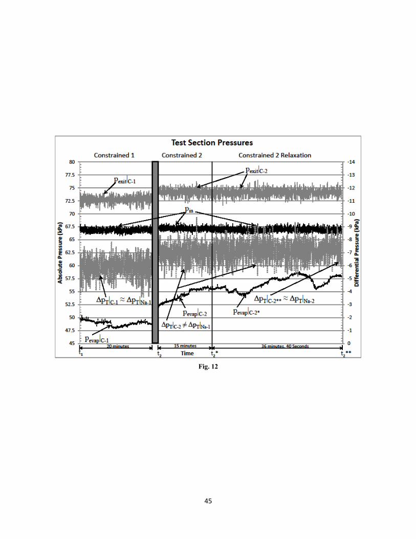
45  

Fig. 12

46  

Fig. 13