
Experimental nonlinear control for flutter suppression in...
40
Experimental nonlinear control for flutter suppression in a nonlinear aeroelastic system Shakir Jiffri 1 , Sebastiano Fichera 2 and John E. Mottershead 3 University of Liverpool, Liverpool, England L69 3GH, United Kingdom Andrea Da Ronch 4 University of Southampton, Southampton, England SO17 1BJ, United Kingdom Experimental implementation of input-output feedback linearisation in controlling the dynamics of a nonlinear pitch-plunge aeroelastic system is presented. The control objective is to linearise the system dynamics and assign the poles of the pitch mode of the resulting linear system. The implementation (a) addresses experimentally the general case where feedback linearisation based control is applied using as the output a degree-of-freedom other than that where the physical nonlinearity is located, using a single trailing-edge control surface, to stabilise the entire system, (b) includes the unsteady effects of the aerofoil’s aerodynamic behaviour, (c) includes the embedding of a tuned numerical model of the aeroelastic system into the control scheme in real-time and (d) uses pole-placement as the linear control objective, providing the user with flexibility in determining the nature of the controlled response. When implemented experimentally, the controller is capable of not only delaying the onset of LCO (Limit Cycle Oscillation), but also successfully eliminating a previously established LCO. The assignment of higher levels of damping results in notable reductions in LCO decay times in the closed-loop response, indicating good controllability of the aeroelastic system and also effectiveness of the pole-placement objective. The closed-loop response is further improved by incorporating adaptation so that assumed system 1 Lecturer, Centre for Engineering Sustainability, School of Engineering, Brownlow Hill. 2 Lecturer, Centre for Engineering Dynamics, School of Engineering, Brownlow Hill. 3 Alexander Elder Professor of Applied Mechanics, Head of the Centre for Engineering Dynamics, School of Engineering, Brownlow Hill. 4 Lecturer, Faculty of Engineering and the Environment, University Road.
Transcript of Experimental nonlinear control for flutter suppression in...

Experimental nonlinear control for flutter suppression
in a nonlinear aeroelastic system
Shakir Jiffri1, Sebastiano Fichera2 and John E. Mottershead3 University of Liverpool, Liverpool, England L69 3GH, United Kingdom
Andrea Da Ronch4 University of Southampton, Southampton, England SO17 1BJ, United Kingdom
Experimental implementation of input-output feedback linearisation in controlling the
dynamics of a nonlinear pitch-plunge aeroelastic system is presented. The control objective
is to linearise the system dynamics and assign the poles of the pitch mode of the resulting
linear system. The implementation (a) addresses experimentally the general case where
feedback linearisation based control is applied using as the output a degree-of-freedom other
than that where the physical nonlinearity is located, using a single trailing-edge control
surface, to stabilise the entire system, (b) includes the unsteady effects of the aerofoil’s
aerodynamic behaviour, (c) includes the embedding of a tuned numerical model of the
aeroelastic system into the control scheme in real-time and (d) uses pole-placement as the
linear control objective, providing the user with flexibility in determining the nature of the
controlled response. When implemented experimentally, the controller is capable of not only
delaying the onset of LCO (Limit Cycle Oscillation), but also successfully eliminating a
previously established LCO. The assignment of higher levels of damping results in notable
reductions in LCO decay times in the closed-loop response, indicating good controllability of
the aeroelastic system and also effectiveness of the pole-placement objective. The closed-loop
response is further improved by incorporating adaptation so that assumed system
1 Lecturer, Centre for Engineering Sustainability, School of Engineering, Brownlow Hill. 2 Lecturer, Centre for Engineering Dynamics, School of Engineering, Brownlow Hill. 3 Alexander Elder Professor of Applied Mechanics, Head of the Centre for Engineering Dynamics, School of
Engineering, Brownlow Hill. 4 Lecturer, Faculty of Engineering and the Environment, University Road.

parameters are updated with time. The use of an optimum adaptation parameter results in
reduced response decay times.
Nomenclature
( ) ( ),′ ′′i i = first, second derivatives with respect to non-dimensional time τ
( ) ( ),⌢i iɶ = assumed, erroneous parameter(s)/variable(s) respectively, in adaptive theory
α = pitch displacement angle / angle of attack (rad)
3 5,α αβ β = pitch non-dimensionalised nonlinearity parameters (-)
3 5,ξ ξβ β = plunge non-dimensionalised nonlinearity parameters (-)
Γ = weighting matrix used in definition of Lyapunov function for adaptive theory
αζ = pitch mode damping ratio (-)
ξζ = plunge mode damping ratio (-)
CLζ = damping ratio assigned to pitch mode during pole-placement
θ = vector containing model parameters that will undergo adaptation
µ = ratio of mass of aerofoil section and other rotating parts to the
mass of a cylinder of air with diameter 2b , 2rotm bπρ (-)
ξ = non-dimensional plunge displacement, /h b (-)
τ = non-dimensional time, /tU b
αω = uncoupled pitch mode natural frequency about elastic axis, K Iα α (rad/s)
ξω = uncoupled plunge mode natural frequency for mass rotm , rotK mξ (rad/s)
ω = ratio of ξ αω ω (-)
cω = Butterworth low-pass filter cut-off frequency (rad/s)
,n CLω = natural frequency assigned to pitch mode during pole-placement

a = non-dimensional distance between semi-chord and elastic axis (-)
b = semi-chord of aerofoil section (m)
c = non-dimensional distance between semi-chord and control surface hinge line (-)
Cα = torsional damping coefficient about rotation axis, per unit span
Cξ = plunge damping coefficient, per unit span
,L mC C = lift and pitch moment coefficients
C = damping matrix
h = plunge displacement (m)
Iα = moments of inertia of aerofoil section and other rotating parts, per unit span (kgm)
Kα = torsional stiffness about rotation axis, per unit span (kgm/s2)
Kξ = plunge stiffness, per unit span (kg/ms2)
3 5,K Kξ ξ = plunge nonlinear stiffness coefficients, per unit span (kg/m3s-2, kg/m5s-2)
plnm = mass of aerofoil section and other parts undergoing plunge, per unit span (kg/m)
rotm = mass of aerofoil section and other rotating parts, per unit span (kg/m)
mɶ = /pln rotm m (-)
M = mass matrix
P = positive definite matrix used in definition of Lyapunov function for adaptive theory
Q = positive definite matrix used adaptive theory, constrained by P
rα = radius of gyration, normalised by b , 2rotI m bα (-)
s = span of aerofoil section (m)
Sα = static moments of aerofoil section and other rotating parts, with respect to
rotation axis, per unit span (kg)
t = time (s)
U = freestream speed (m/s)

*U = reduced speed, /U b αω
V = scalar quadratic Lyapunov function used in adaptive theory
xα = centre of mass of aerofoil section from rotation axis, normalised by b , rotS m bα (-)
I. Introduction
EROSPACE engineering is an area that has continued to see adaptation, rapid growth and innovation in
response to the particular demands and constraints arising during a given era. Present-day turbofan engines, for
instance, are 90 times more powerful compared to their predecessors from the 1940s, yet are 70% more fuel efficient
[1]. Increased use of lightweight composite materials in recent times has resulted in a reduction in aircraft weight.
The main trends of today are in working towards improved fuel efficiency, higher speeds, reduced weight, and
increased electrification. These trends are driven by factors such as the effort to reduce travel times, increase
business productivity, and of course the over-arching need, and ever-growing urgency in tackling emissions and
moving towards greener technologies. Consequently, it is becoming increasingly important to improve modelling
methods and challenge what may be unsound conventions and simplifications made in the past, either due to
pragmatism or lack of suitable methods to handle the complexity of problems that would otherwise have arisen.
Nonlinearity is one such area, whose effects are becoming increasingly evident as we move along the trends
described above. Detailed literature reviews of nonlinearity in aeroelasticity were carried out by Dowell et al. [2]
and Lee et al. [3].
The present work gains motivation by the need for a clearer understanding of the role of nonlinearity within
aeroelasticity. Specifically, this paper relates to the active control of nonlinear aeroelastic systems. Over the past few
years, research conducted at the University of Liverpool has been aimed at addressing the need highlighted above.
Papatheou et al. [4] implemented the Receptance Method [5] experimentally on a linear two degree-of-freedom
aeroelastic system to successfully increase the flutter speed by separating pitch and plunge modes via pole-
placement. Theoretical work and numerical modelling have primarily been on controlling smooth and non-smooth
nonlinear aeroelastic systems by Da Ronch et al. [6] and Jiffri et al. [7]. A sliding mode controller was developed by
Wei and Mottershead [8] based upon passivity principles to ensure a positive rate of energy dissipation in the
presence of bounded nonlinearity uncertainty. Knowledge of the functional form of the nonlinearity was not
required and the method was shown to be robust to bounded input disturbance and measurement noise. More recent
A

experimental developments include measurement of the aeroelastic system’s parameters and open-loop
investigations, experimental testing conducted on piezo-MFC bimorph actuation for morphing wing technology and
the development and manufacture of a flexible wing for aeroelastic testing by Fichera et al. [9].
Elsewhere, several publications on the application of active control on aeroelastic systems have appeared. Of
particular importance is a series of collections of publications [10-12] on research conducted under the Benchmark
Active Control Technology (BACT) project at NASA Langley Research Centre, with involvement from a number of
leading universities and aerospace-related companies. The project focused on a two-degree-of-freedom pitch-plunge
aerofoil, and studied the effects of unsteady aerodynamics and active control methods. Frampton et al. [13] designed
and investigated experimentally an LQG compensator for LCO (limit cycle oscillation) suppression and increasing
of the flutter boundary of a three-degree-of-freedom typical section with freeplay in the flap restoring stiffness.
Although the controller was applied successfully to a nonlinear dynamical system, the control design was based on
the linear typical section with no freeplay. Kelkar and Joshi [14] presented a passivity-based controller design for
non-passive linear, time-invariant systems. They investigated different methods of passification and applied this
controller design approach to the BACT wing (linear) model. Mukhopadhyay [15] developed a transonic flutter
suppression control law using a unified LQG and minmax method. The control algorithm was successfully tested
experimentally on the BACT rig, proving to be able to increase the closed-loop flutter dynamic pressure by over
50% up to the wind-tunnel upper limit. Prasanth and Mehra [16] studied active control of nonlinear aeroelastic
systems based on energy flow. The design techniques were applied to a numerical nonlinear version of the BACT
wind-tunnel model. The main limitation of this approach lies in the need to gain access to generalized velocities
and/or displacements for feedback. Xing and Singh [17] developed a new adaptive control law for the control of
nonlinear aeroelastic systems using only output feedback based on backstepping design techniques. They performed
numerical simulations on a two degree-of-freedom system with a polynomial nonlinearity in the pitch stiffness.
Bendiksen [18] adopted a more general view of the mechanism of flutter, as compared to the classical frequency
coalescence description. The general interpretation, based on a nonlinear aerodynamic work functional defining the
flutter subspace, provided the basis for a control approach that is based on altering a critical aeroelastic mode, as
opposed to the traditional approach of frequency separation. In [19], Haley and Soloway developed a generalised
predictive controller (GPC) for flutter suppression, and implemented this in both simulation and experiment. The
controller was based on minimising a cost function involving predicted responses of the system and also control
effort. In the simulation case, a linear model of the BACT wing was used. The effectiveness of the controller was
illustrated by application in both simulation and experiment, to successfully suppress flutter in both cases, for the
flight conditions considered. Waszak [20] presented the development, simulation and experimental testing of a
robust MIMO multi-variable control law using trailing edge and upper-spoiler controllers to suppress flutter, in the
presence of uncertainty. It was found that the multi-variable controller performed successfully in suppressing flutter
- notwithstanding minor difficulties arising from practical implementation issues - and had superior stability and
performance robustness compared to SISO control.
Also related to the BACT model – not part of the collections [10-12] mentioned earlier - is the work by Mason
et al. [21, 22], where a methodology was developed for designing robust multirate controllers. Application of such a
multirate controller for flutter suppression, based on a representative linear numerical model (including unsteady
aerodynamics), was demonstrated on the BACT wing. The advantage of multi-rate designs is that although the
design of the controller is more complex, the number of real-time computations and/or hardware is reduced.
The concept of so-called ‘fly-by-feel’ was established in a series of papers by Suryakumar and his colleagues
[23-25]. They departed from the conventional model-based approach that makes use of kinematic states such as the
aircraft angle of attack, instead using critical aerodynamic flow features (CAFFI), in particular the leading edge
stagnation point (LESP), the position of which is now measurable by using distributed hot-film sensors. Suryakumar
et al. [23] derived a simple model relating the stagnation point to the lift of an aerofoil undergoing unsteady
manoeuvres. The application of the model in flutter control is described in detail in [25], where an approach,
guaranteed to be dissipative, was developed based on the aerodynamic work done on a nonlinear wing section. The
analysis does not require knowledge of the free-stream and structural dynamics and the transition from stable to
unstable regions does not necessarily imply the existence of flutter, but provides the conditions under which flutter
could possibly occur. A spanwise-distributed, co-located sensing and control architecture using load-based feedback
and the low-order controller [25] is described and implemented in [24].
Of more relevance to the present work is a series of publications by Strganac and colleagues [26-31], in which
the application of active control on aeroelastic systems with hardening-type structural nonlinearities has been
investigated both theoretically and also experimentally, through the use of quasi-steady aeroelastic models. These
studies utilised the feedback linearisation nonlinear control method, in conjunction with LQR control as the linear
control objective. The authors of the present article are motivated by these findings, and further explore feedback

linearisation based aeroelastic control, with some notable differences in the overall scheme. This article presents
experimental results on the closed-loop active control of nonlinear aeroelastic flutter, and thereby aims to enrich the
knowledge base in nonlinear aeroelasticity, particularly relating to control. The originality of this work stems from
(i) experimental demonstration of stabilisation and pole placement in an under-actuated two-degree of freedom
aerofoil system by feedback linearisation using a single control surface; whereas, this has been done previously for
the special case when the output is chosen at the same degree of freedom as the nonlinearity – so that the
nonlinearity is cancelled exactly – in this research the general case is considered when the degree of freedom at the
nonlinearity is not available for measurement (resulting in the zero-dynamics being nonlinear), (ii) the real-time use
of a low-order numerical model which enables the inclusion of unsteady aerodynamic effects (improving model
accuracy) in the control process, and the ability of the controller to completely eliminate a fully developed LCO, and
(iii) the use of pole-placement as the linear control objective, which, although more challenging to implement
experimentally, has advantages over LQR control such as providing the user more flexibility in adjusting specific
dynamic parameters, and removing the need to determine appropriate weighting factors that are required in LQR
control. The advantage of obtaining aerodynamic loads indirectly through the aeroelastic response, as mentioned in
(ii) above, is that no changes or modifications to an experimental aeroelastic apparatus are needed. Measurement
sensors are widely used and non-intrusive. More generally, this approach goes in the direction of embedding a
reduced order model in real-time to monitor quantities of interest on the airframe, specifically for gust loads [32].
An alternative to the indirect approach is that proposed, for example, in [25], mentioned above.
The research presented in this paper extends previous work relating to the two degree-of-freedom aeroelastic
system at the University of Liverpool mentioned above. Numerical simulations of closed-loop control presented in
[6] are implemented experimentally, utilising previously obtained experimental measurements and open-loop
results. §II describes the experimental setup, which is followed by a detailed description of the low-order numerical
model (§III) used in conjunction with the experimental work. A description of the procedure followed in setting the
parameters of the numerical model is given in §IV, followed by the procedure involved in embedding the numerical
model in the control loop, in §V. The main results are then presented in §VI, prior to the final section VII which
draws the main conclusions of this work.

II. Experimental Setup
The experiments discussed in this paper have been performed on a two degree-of-freedom pitch-plunge aerofoil
section mounted in a low-speed wind tunnel at the University of Liverpool (Fig. 1). The dimensions of the wind
tunnel test section are 1.2 m × 0.4 m × 1.0 m, and the maximum wind speed achievable in the tunnel is
approximately 18 m/s. An assembly consisting of a torque tube and a set of horizontal and vertical linkages support
the aerofoil section in the plunge direction, and prevent span-wise tilting or bending. A dSPACE real-time control
system is utilised for closed-loop control. The inputs to dSPACE are the voltages from three laser displacement
sensors (two Keyence LK-500 sensors, one micro-epsilon OptoNCDT 1402-100 sensor) measuring the vertical
displacement at strategic locations on the aerofoil system, as depicted in Fig. 2. The output from dSPACE is
amplified by two Khron Hite 7500 wideband power amplifiers, to drive a twin piezo-stack arrangement [33, 34] and
actuate a trailing edge flap on the aerofoil. For stepped-sine modal testing of the aeroelastic system, an LMS
SCADAS III data acquisition system is employed. This facility was utilised for objectives such as (i) verifying that
the flexible modes of the aeroelastic system are substantially higher in frequency than those of the pitch-plunge
modes (ii) choosing the pitch and plunge stiffnesses such that flutter is induced within the achievable air speed range
of the wind tunnel (iii) tuning the parameters of the numerical model to match those of the experimental system.

(a) Wind tunnel test section – view 1 (LHS) (b) Wind tunnel test section – view 2 (RHS)
(c) Wind tunnel test section – view 3 (RHS) (d) Tensioned wire design for plunge nonlinear stiffness
Fig. 1 Aeroelastic system experimental setup
(e) V-stack trailing edge flap actuator
7 1
2 5
8
6
9
(1) aerofoil vertical support (2) housing (3) aerofoil section (4) trailing edge control surface (5) plunge spring - linear (6) laser displacement sensors (7) torsion bar (8) pitch spring (9) plunge spring - nonlinear (10) piezo-stack actuators ( located inside (4) )
4
3
10

Fig. 2 Measurement locations on aeroelastic system
The aerofoil section has a NACA 0018 profile, with a chord length of 0.35 m and a span of 1.2 m. It is equipped
with a trailing edge flap, located centrally, having chord-wise and span-wise dimensions 25% and 35%, respectively,
with respect to aerofoil chord and span. The flap is capable of rotating approximately ±5˚, up to a bandwidth of
approximately 15 Hz (although the flap has been operated up to 30 Hz at lower amplitudes). Adjustable leaf springs
provide stiffness to the aerofoil, independently in the plunge and pitch directions. A structural nonlinearity is
incorporated into the system in the form of a hardening polynomial stiffness in the plunge degree-of-freedom. This
is achieved by the clamped-clamped tensioned wire arrangement depicted in Fig. 1 (d). The force-displacement
relationship may be expressed as
3 5
3 5,nlF K h K h K hξ ξ ξ= + + (1)
where all stiffness coefficients 3 5
, ,K K Kξ ξ ξ of the various powers of the plunge term h are positive, and are readily
measured via a static force/displacement test. The flap is the only means of input to the system during closed-loop
control, and it is actuated by a mechanically amplified “V-stack” piezoelectric stack arrangement [33, 34] as
depicted in Fig. 1 (e). The control law computes the required action by the flap, based on pitch and plunge
deflections and velocities, and also aerodynamic states (addressed later) of the aerofoil section. Deflections are
computed by combining basic geometry with the laser sensor readings, whereas velocities are obtained by
Point #3
Point #2
Point #1

numerically differentiating the displacements. Some filtering of the displacement signals is required prior to
differentiation; specifically, a second-order Butterworth low-pass filter with cutoff frequency 15 Hz is used. The
controller then outputs the appropriate voltage signal from dSPACE, which once amplified, is directed to the piezo-
stacks in the V-stack actuator, causing rotation of the flap.
III. Unsteady Aeroelastic Numerical Model
In this section a twelve-state numerical model is presented with four structural and eight aerodynamic states. The
aerofoil section shown in Fig. 3 has two degrees of freedom that define the motion about a reference elastic axis
(e.a.). The plunge deflection is denoted by h, positive downward, and α is the angle of attack about the elastic axis,
positive with nose up. The motion is restrained by two springs, of stiffness Kξ and Kα , and is assumed to have a
horizontal equilibrium position at 0h α= = . Structural damping in both degrees of freedom is also included in the
system. A trailing-edge flap, which is assumed massless in this study, is used in combination with an active control
system as the input to the aeroelastic system.
Fig. 3 Schematic of a two-degree of freedom aeroelastic system;
the wind velocity is to the right and horizontal
The motion of the system, without control surface dynamics and with a linear structural model, is described [35]
in non–dimensional form by
cb
undeformed position
e.a. c.g.

( )
( )( )( )
2
2
2 12**
22 21* *
00.
01 0
xLUUr
mrU U
Cm
Cx
ξα
αα
α
ζ ω ωπµ
ζ ωπµα
τξ ξ ξτα α α
− ′′ ′ + + = ′′ ′
ɶ
(2)
The lift coefficient, LC , is defined positive upward according to the usual sign convention in aerodynamics. The
plunge displacement is positive downward; hence the negative sign in front of LC in eq. (2). Non-dimensional
parameters are defined in the nomenclature. Note also that the above equations are formulated in terms of a non–
dimensional time, τ , based on the aerofoil semi–chord and freestream speed, /tU bτ = . The prime notation
( ) , ( )′ ′′i i , used throughout this paper, indicates differentiation with respect to non-dimensional time τ , instead of
the well-known dot notation which is often used to denote differentiation with respect to absolute time t . The above
model of the pitch–plunge aerofoil system, with an appropriate model of the aerodynamics, is used in this work to
simulate the dynamics of the wind tunnel nonlinear aeroelastic test rig. Theoretical detail on the aerodynamics used
in this model including its mathematical formulation have been derived previously [6]. The end result is an
aeroelastic model that approximates the unsteady aerodynamic behaviour using additional state variables. The
coupled model consists of 12 state variables, eight of which are aerodynamic states required to model the unsteady
aerodynamics as described above, and the remaining four which are structural states. The trailing–edge flap rotation
is used as control input. The state vector (of dimension 12) is defined as,
{ } { }1 2 3 4 5 6 7 8 1 2 12 ,T T
w w w w w w w w x x xα α ξ ξ′ ′= ⇒ =x x ⋯ (3)
where the structural states , , ,α α ξ ξ′ ′ are pitch deflection and velocity, non-dimensional plunge displacement
( )/h b and velocity respectively, the aerodynamic states 1 2,w w are associated with pitch motion, 3 4,w w with
plunge motion, 5 6,w w with flap motion and 7 8,w w with gusts. Then, the coupled system of equations, with the
dependence on non-dimensional time τ omitted for brevity, may be cast in the nonlinear state-space form
( ) ,u′ = +x f x g (4)

where
( )
{ }( )
( )
( )
2
2 2
4
4 4
1 1 5
1 2 6
3 1 71 2 12
3 2 8
1 9
2 10
3 11
4 12
0
0
0
0, , , ,
0
0
1
1
0
0
T
x
f g
x
f g
x xu x x
ux xx x xx x
x
x
x
x
εε
δεε
εεεε
− ′ = + − = = = −= − − − − −
x
x
x f x gf x g
x ⋯
(5)
( ) ( )
[ ] [ ]
3 3 5 3 3 51:12 1,3 1 3,3 3 1,5 1 1:12 1,3 1 3,3 3 1,5 1
2 45 53,5 3 3,5 3
1:12 1 2 12 1:12 1 2 12 2 4
, ,
, , , .
T T
T T
x x x x x xf f
x x
g g
δ δ δ δ
δ δ
λ λ λ γ γ γλ λ δ λ δ γ γ δ γ δ
λ λ λ γ γ γ λ γ
′ ′′ ′ ′′
+ + + + + + = = ′ ′′ ′ ′′+ + + + + +
= = = =
λ x γ xx x
λ γ⋯ ⋯
(6)
The term ( )f x is a nonlinear function of the state vector x , and u represents the flap rotation δ . The
coefficients of the above aeroelastic system are detailed partly in [6] and partly in the Appendix at the end of this
paper. This allows one to setup the numerical model starting from the baseline aeroelastic parameters of the pitch–
plunge aerofoil described later on. In this model, the input to the system is the flap rotation angle δ . Since the
terms ,δ δ′ ′′ are merely time-derivatives of the input, they are not independent of δ and therefore are not treated as
additional inputs, but rather as time-varying quantities that are part of the system (hence located inside ( )f x ).
These quantities may be computed by numerical differentiation of .δ It was found in simulation that their effect
was small and in experimental practice they gave rise to undesirable amplification of noise resulting in high
frequency components in the flap motion. The ,λ γ terms arise from the linear combinations in the expressions for
2 4,x x′ ′ , appearing in [6], and are given by eq. (A2.2) and (A2.3) respectively in Appendix A2. Gust inputs, which
would normally appear in the expressions relating to 11 12,x x′ ′ , have not been considered in this work. Thus, the state
variables 11 12,x x will remain identically zero in all simulation results presented in this paper.

IV. Numerical Model Parameters
This section explains the procedure by which the parameters describing the dynamical behaviour of the
aeroelastic system were determined for reproduction of this behaviour in the numerical model. The relevant
parameters of the numerical model (described in §III) were set to the values measured/acquired from wind tunnel
tests. Subsequently, fine tuning of these parameters was performed such that the discrepancy between both the linear
and nonlinear dynamic behaviour of the numerical model and the aeroelastic system was minimised. The resulting
model is a simplification of the more complicated physical system, not least in that the actuation of the flap by the
V-stack actuator is known to possess a degree of freeplay and Coulomb friction (see Appendix A3), so that even
when the tensioned wire is removed, the system remains nonlinear (albeit in a different way) whereas the model,
which neglects the freeplay effect, is strictly linear. Thus the resulting set of parameters represent a compromise
between physical reality and a model that offers a reasonable fit. Table 1 contains the finalised parameter values,
where the format in which they are presented follows that used by [36, 37] and many others. A definition of these
parameters is also provided in the Nomenclature section of the present article, for the reader’s convenience.
Table 1 Aeroelastic model parameter values
Parameter Value Parameter Value Parameter Value
αω (rad/s) 29.13955 a -0.32571 αζ 0.0115
rα 0.5 c 0.5428 pln rotm m m=ɶ 2.21669
xα 0.021 b (m) 0.175 3ξβ 1085.62
ξω (rad/s)
(linear/nonlinear)
24.64246 /
26.41656 µ 30
5 3 5, ,ξ α αβ β β 0
ω
(linear/nonlinear)
0.84567 /
0.90655 ξζ 0.0175
The non-dimensional nonlinearity coefficients 3 5 3 5, , ,ξ ξ α αβ β β β are derived from eq. (1), knowing the semi-
chord b (see Appendix A3). The different values for ξω (and ω ) in the linear and nonlinear cases arises from the
tensioned wire design of the nonlinear structural stiffness described in §II. When the tensioned wire is attached to
the aerofoil, in addition to the nonlinear terms, a component of linear stiffness is also introduced. It is this additional
linear stiffness that increases ξω (and therefore ω ) in the underlying linear behaviour of the nonlinear system.
A. Measurement of parameters
A combination of methods was employed during acquisition of the aeroelastic system’s parameters. Values of
stiffness in the pitch and plunge directions were measured from static force/displacement tests, including the
nonlinear plunge stiffness. Modal tests performed with pitch and plunge constrained in turn provided natural
frequencies and damping ratios (,α ξζ ζ ) for pitch and plunge motion. Estimation of the plunge mass and pitch
moment of inertia was achieved by combining the natural frequencies with the stiffness values measured as
explained above. The mass undergoing pure rotation ( rotm ) was measured via a static moments test with the pitch
spring disconnected. This value, combined with the plunge mass enabled computation of the plunge/pitch mass ratio
mɶ . The static moments test was also used to compute xα . Quantities such as 3
, , ,rα ξ α ξω ω β were computed from
the various measurements described thus far. Distances such as , ,a c b were obtained by direct measurement.
B. Tuning of measured parameters
The responses simulated using the measured parameters, for both linear and nonlinear cases were compared with
the respective measured responses from the aeroelastic system. Although a good match was obtained, as expected
discrepancies between the respective responses were observed. The overall tuning objective in this case was to make
adjustments to the measured parameters so as to reduce the model/aeroelastic system discrepancies both in the linear
and nonlinear cases. A sensitivity study was undertaken to understand the effect on the response of varying a given
parameter. A series of numerical simulations was carried out, and a given parameter varied at any one time. A
qualitative summary of the trends identified from this study may be found in Appendix A5. During initial tuning
attempts, it was noted that some of the requirements were conflicting, therefore a compromise between satisfying
linear and nonlinear response matching was required. The final tuned set of parameters was decided upon once such
a good balance was deemed to have been achieved.
C. Comparing performance of tuned numerical model with aeroelastic system
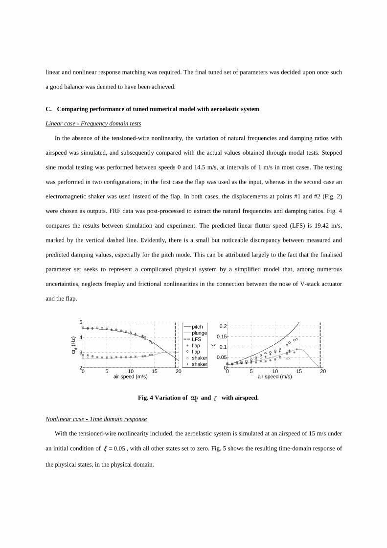
Linear case - Frequency domain tests
In the absence of the tensioned-wire nonlinearity, the variation of natural frequencies and damping ratios with
airspeed was simulated, and subsequently compared with the actual values obtained through modal tests. Stepped
sine modal testing was performed between speeds 0 and 14.5 m/s, at intervals of 1 m/s in most cases. The testing
was performed in two configurations; in the first case the flap was used as the input, whereas in the second case an
electromagnetic shaker was used instead of the flap. In both cases, the displacements at points #1 and #2 (Fig. 2)
were chosen as outputs. FRF data was post-processed to extract the natural frequencies and damping ratios. Fig. 4
compares the results between simulation and experiment. The predicted linear flutter speed (LFS) is 19.42 m/s,
marked by the vertical dashed line. Evidently, there is a small but noticeable discrepancy between measured and
predicted damping values, especially for the pitch mode. This can be attributed largely to the fact that the finalised
parameter set seeks to represent a complicated physical system by a simplified model that, among numerous
uncertainties, neglects freeplay and frictional nonlinearities in the connection between the nose of V-stack actuator
and the flap.
Fig. 4 Variation of dω and ζ with airspeed.
Nonlinear case - Time domain response
With the tensioned-wire nonlinearity included, the aeroelastic system is simulated at an airspeed of 15 m/s under
an initial condition of 0.05ξ = , with all other states set to zero. Fig. 5 shows the resulting time-domain response of
the physical states, in the physical domain.
0 5 10 15 202
3
4
5
air speed (m/s)
ωd (
Hz)
0 5 10 15 200
0.05
0.1
0.15
0.2
air speed (m/s)
ζ
pitchplungeLFSflapflapshakershaker
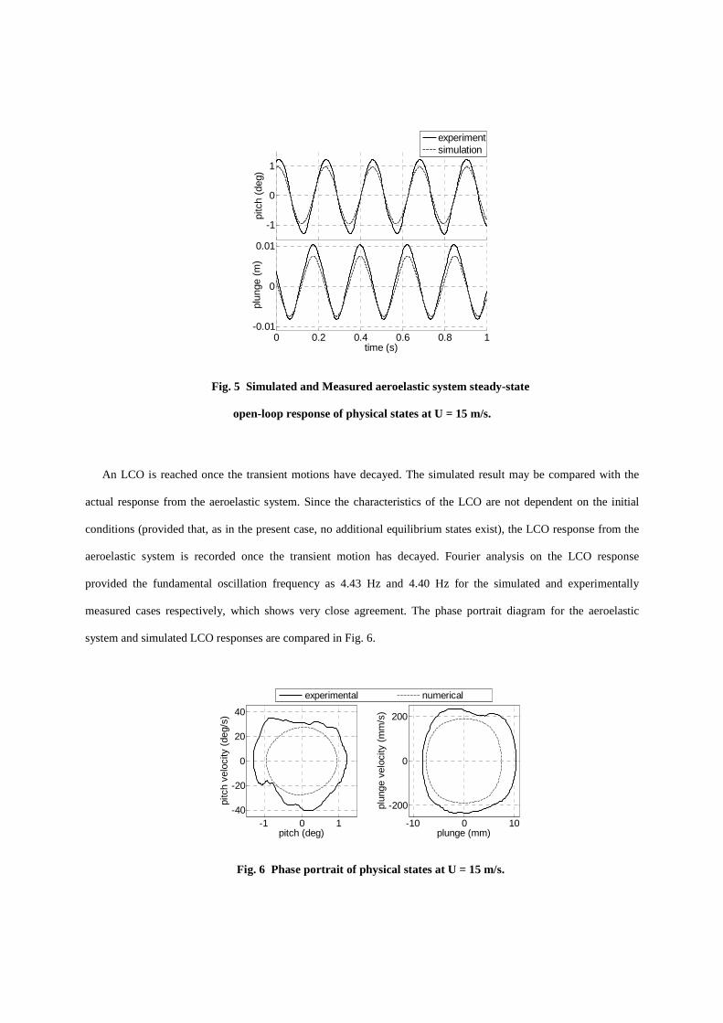
Fig. 5 Simulated and Measured aeroelastic system steady-state
open-loop response of physical states at U = 15 m/s.
An LCO is reached once the transient motions have decayed. The simulated result may be compared with the
actual response from the aeroelastic system. Since the characteristics of the LCO are not dependent on the initial
conditions (provided that, as in the present case, no additional equilibrium states exist), the LCO response from the
aeroelastic system is recorded once the transient motion has decayed. Fourier analysis on the LCO response
provided the fundamental oscillation frequency as 4.43 Hz and 4.40 Hz for the simulated and experimentally
measured cases respectively, which shows very close agreement. The phase portrait diagram for the aeroelastic
system and simulated LCO responses are compared in Fig. 6.
Fig. 6 Phase portrait of physical states at U = 15 m/s.
-1
0
1
pitc
h (d
eg)
0 0.2 0.4 0.6 0.8 1-0.01
0
0.01pl
unge
(m
)
time (s)
experimentsimulation
-1 0 1-40
-20
0
20
40
pitch (deg)
pitc
h ve
loci
ty (
deg/
s)
experimental numerical
-10 0 10
-200
0
200
plunge (mm)
plun
ge v
eloc
ity (
mm
/s)

It is evident from the above figures that there is good agreement between the aeroelastic system and the tuned
numerical model, notwithstanding the apparent presence of additional harmonics in the experimental pitch phase
portrait plot. Again, frictional and freeplay effects in the aeroelastic system – absent in the numerical simulation –
would partly contribute to the discrepancies observed in Fig. 6.
V. Embedding Numerical Model in the Aeroelastic System Control Loop
The control laws that will be applied in the aeroelastic system in this work are to be synthesised from the 12-state
numerical model described in §III. When implemented, the state-feedback controller will require access to all 12
states in real-time. The four structural states may be obtained from direct measurement of pitch and plunge, and their
time derivatives. The remaining eight aerodynamic states may not be measured directly; it therefore becomes
necessary to acquire them by other means. In the present work, this objective is fulfilled by embedding the numerical
model in the experimental control loop and utilising it to generate in real time the aerodynamic states. The measured
flap deflection angle – i.e. the physical implementation of the input to the aeroelastic system - is directed to the
embedded numerical model, which then generates in real-time the full 12-state vector. The first four entries of this
vector – i.e. the structural states – are then replaced by the measured values to create a “hybrid” state vector which is
the basis on which the control input is computed. The hybrid vector is then fed back into the embedded numerical
model (along with the flap deflection angle) which allows computation of the state vector at the next time step.
Fig. 7 depicts a simplified schematic of the control strategy adopted in this work. An explanation of the
purpose/function of each block is now presented, where it should be noted that the numbering does not necessarily
reflect the sequence of steps.

Fig. 7 Schematic of control strategy
(1) The displacements at points #1, #2 and #3 from the three laser displacement sensors (Fig. 2) are read into
dSPACE, and passed through second-order Butterworth low-pass filters to remove noise.
(2) The displacements at points #1 and #2 are converted into pitch angle (rad) and non-dimensional plunge
ξ , then differentiated with respect to time to compute velocities.
(3) The flap rotation angle δ is computed through knowledge of pitch angle, plunge displacement and the
displacement at point #3.
(4) The embedded numerical model generates the full state vector x based on knowledge of the measured
structural states 1 4x x− and also the actual flap rotation δ .
(5) The aerodynamic states 5 12x x− are picked from the full state vector x generated by the embedded numerical
model.
(6) Once the measured structural states 1 4x x− are combined with the numerical aerodynamic states 5 12x x− to
form the new “hybrid” state vector xɶ , the artificial inputs ([6]) are computed
(7) The actual, nonlinear input is computed
(8) The output from dSPACE is sent to the piezoelectric actuator of the flap to effect the required rotation.
(7)
dSPACE
output
(1)
dSPACE
inputs
(2)
compute
structural
states
(5)
compute
artificial
inputs
(4)
select
x5-x12
(6)
compute actual
(nonlinear)
input (3)
numerical
aeroelastic
model
x1-x4

The time step between measurements is 0.001 seconds, which is determined by the data acquisition / control
system (in this case dSPACE). Thus, the embedded numerical model and, in fact, the entire control loop depicted in
Fig. 7 are evaluated once every 0.001 seconds. This time interval is adequately small to ensure a smooth variation of
the state variables that are computed by the model through numerical integration.
VI. Results
In this section, experimental results from the aeroelastic system and related simulation results from the numerical
model are presented. Open-loop results from the embedded numerical model are discussed initially, followed by
closed-loop results with the nonlinear controller implemented. Predictions from numerical simulations are compared
with experimental measurements.
A. Open loop system – embedded model
A comparison between the open-loop response of the structural states of the aeroelastic system and the numerical
model was carried out in §IV.C earlier. It is relevant to also compare the aerodynamic states generated by the online,
embedded numerical model with those obtained from an offline simulation using the numerical model. This
comparison is made in Fig. 8.
Fig. 8 Aerodynamic states at U = 15 m/s.
-0.05
0
0.05
x 5
-0.05
0
0.05
x 6
-0.4
0
0.4
x 7
-0.1
0
0.1
x 8
0 0.2 0.4 0.6 0.8 1-0.04
0
0.04
time (s)
x 9
0 0.2 0.4 0.6 0.8 1
-0.01
0
0.01
time (s)
x 10
real-time embedded model offline numerical model

It can be seen that there is good agreement between both cases for 5 6 8, ,x x x . The most likely cause for the
mismatch observed in the case of 7x is the asymmetry in the plunge displacement LCO with respect to the zero
position (this can be observed in Fig. 5(b) in §IV above). In 9 10,x x , the reason for the result from the offline
numerical model being zero is the zero deflection angle of the flap (uncontrolled case). However in reality, there
will always be some rotation of the flap (even when it is not actuated) due to freeplay effects, hence the non-zero
response in the case of the real-time embedded model response. The final two aerodynamic states 11 12,x x (not
shown here) are exactly zero in both cases, as gust loads are not considered in this work.
B. Closed loop system
In this section, one examines the behaviour of the system with the nonlinear controller based on feedback
linearisation implemented, prior to which a verification of the stability of the internal dynamics is carried out.
Pitch linearisation internal dynamics
The stability of the internal dynamics resulting from pitch linearisation is verified by studying the stability of the
zero dynamics (see [6]). Time-domain simulations of the zero dynamics are carried out repeatedly, with a random
set of initial conditions each time. In all cases, all 10 states of the zero dynamics decay to zero, indicating
asymptotically stable behaviour. It is of interest to study the dynamics of the underlying linear system. Evaluated
about a given equilibrium point, stability properties of the point may be revealed from the eigenvalues of the
Jacobian [38]. In the present case, it can be concluded from inspection that the origin is an equilibrium point of the
zero dynamics. The eigenvalues of the Jacobian evaluated at the origin, given below, all have negative real parts
indicating asymptotic stability.
-0.042723537810 -0.262637592121 -0.04550000000 -0.015619146610 -0.300000000000
-0.139300000000 -1.802000000000 -0.04550000000 -0.015619146610 -0.300000000000
Since the internal dynamics have been verified as being stable, one may proceed with pitch output linearisation.

Pole-placement via feedback linearisation
Firstly, it is necessary to establish a control aim. In the present case, it would be appropriate to suppress the LCO
response by eliminating the underlying nonlinearities in the system. This aim may be achieved by applying a
controller that provides linearising feedback to cancel out the nonlinear behaviour of the system.
As for the linear part of the controller, it is sought to modify the dynamics of the controlled pitch sub-system by
applying pole-placement. Specifically, the pole-placement objective in the present exercise is to increase the
damping in the pitch system, which should now, in theory, be decoupled from the overall aeroelastic system as a
result of the linearising feedback (provided accurate modelling of the system parameters, including nonlinearity
parameters). With the system undergoing LCO, the controller was implemented with a desired value of the pitch
damping ratio ( CLζ ) specified. Fig. 9 shows the pitch and plunge responses for CLζ = 0.3, where the controller is
switched on at exactly three seconds.
Fig. 9 Closed-loop response of aeroelastic system for CLζ = 0.3, at U = 15 m/s.
It is evident that once activated, the controller successfully suppresses the LCO and drives the response to the
origin in just under five seconds. Repeatability of the above behaviour was verified by carrying out the same test
multiple times and ensuring a consistent outcome. In the simulated responses shown in the bottom half of Fig. 9, the
effect of the Butterworth low-pass filters has been included for consistency when comparing with experimental
measurements. A comparison of the measured responses with the predicted ones – where the controller is activated at
-1
0
1
pitc
h (d
eg)
measuredcontroller ON
-0.01
0
0.01
plun
ge (
m)
measuredcontroller ON
2 3 4 5 6 7 8
-1
0
1
pitc
h (d
eg)
time (s)
2 3 4 5 6 7 8-0.01
0
0.01
plun
ge (
m)
time (s)
predictedcontroller ON
predictedcontroller ON

the same point along a given cycle as in the experimental case, for consistency in comparison - yields that in the latter
case, significantly less time is required for the response to decay. A variety of reasons may be contemplated for the
discrepancy, such as the loss of accuracy during computation of pitch and plunge deflections, introduction of noise
during numerical differentiation of pitch and plunge to obtain respective velocities. Also, it was confirmed using
offline numerical simulations that the phase delays resulting from filtering of signals required for numerical
differentiation played a small, but significant role in causing this discrepancy. Another major source of discrepancy
could be attributed to the mismatch between the tuned and actual system parameters, resulting in the dynamics not
being cancelled out completely as desired. Consequently, complete uncoupling of the pitch motion from the
remaining dynamics is not achieved; this is reflected in the nature of the measured pitch motion where content from
multiple modes of vibration is evident. However, one may conclude from inspecting the actual closed-loop response
that the extent of this problem is not so great as to prevent the present control method from being implemented with
satisfactory effectiveness. The flap motion during the above control run is presented in Fig. 10.
Fig. 10 Flap motion for closed-loop control of aeroelastic system for CLζ = 0.3, at U = 15 m/s.
Accurate measurement of the flap deflection proved particularly challenging, due to the multiple dimensional
parameters involved in its computation based on displacement readings measured at the three strategic locations. This
partially explains the discrepancy between the measured and simulated cases evident from Fig. 10. Another reason
may be attributed to the correction factor employed in taking into account the (span-wise) length of the control
surface, which is not full-span as in the numerical model. Another issue that is clear from Fig. 10 is the asymmetry in
the motion of the flap, most likely due to freeplay effects in the V-stack and also in the flap itself. Clearly, the above
issues concerning the flap motion will also affect the quality of the closed-loop response (Fig. 9).
2 3 4 5 6 7 8-2
-1
0
1
2
flap
rota
tion
(deg
)
time (s)
2 3 4 5 6 7 8-2
-1
0
1
2
flap
rota
tion
(deg
)
time (s)
measuredcontroller ON
predictedcontroller ON
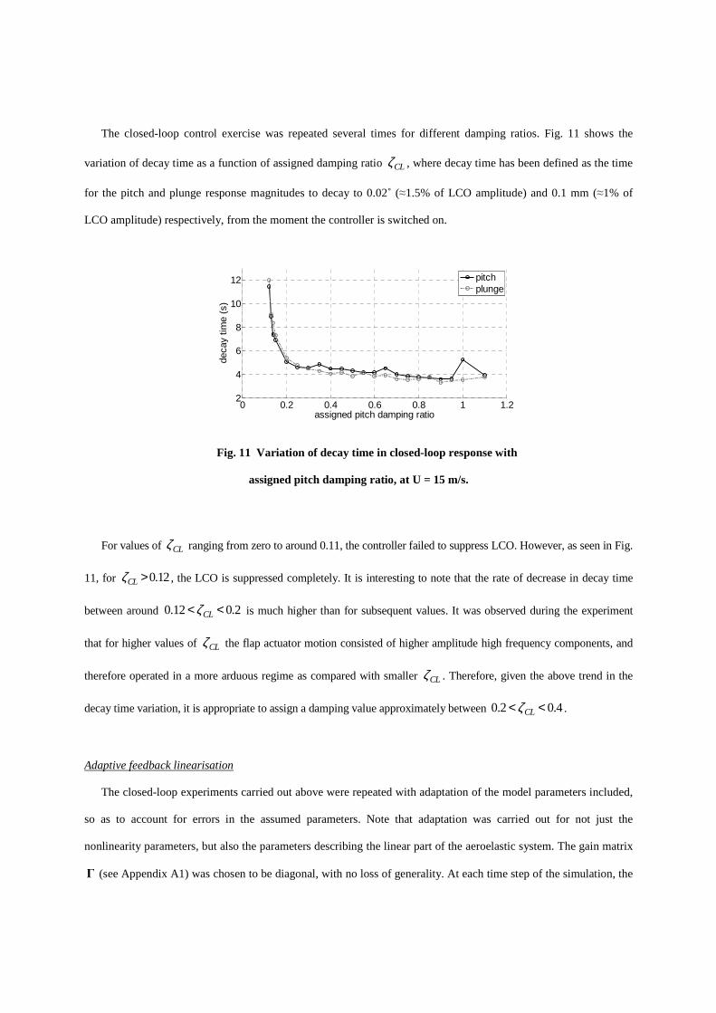
The closed-loop control exercise was repeated several times for different damping ratios. Fig. 11 shows the
variation of decay time as a function of assigned damping ratio CLζ , where decay time has been defined as the time
for the pitch and plunge response magnitudes to decay to 0.02˚ (≈1.5% of LCO amplitude) and 0.1 mm (≈1% of
LCO amplitude) respectively, from the moment the controller is switched on.
Fig. 11 Variation of decay time in closed-loop response with
assigned pitch damping ratio, at U = 15 m/s.
For values of CLζ ranging from zero to around 0.11, the controller failed to suppress LCO. However, as seen in Fig.
11, for 0.12CLζ > , the LCO is suppressed completely. It is interesting to note that the rate of decrease in decay time
between around 0.12 0.2CLζ< < is much higher than for subsequent values. It was observed during the experiment
that for higher values of CLζ the flap actuator motion consisted of higher amplitude high frequency components, and
therefore operated in a more arduous regime as compared with smaller CLζ . Therefore, given the above trend in the
decay time variation, it is appropriate to assign a damping value approximately between 0.2 0.4CLζ< < .
Adaptive feedback linearisation
The closed-loop experiments carried out above were repeated with adaptation of the model parameters included,
so as to account for errors in the assumed parameters. Note that adaptation was carried out for not just the
nonlinearity parameters, but also the parameters describing the linear part of the aeroelastic system. The gain matrix
Γ (see Appendix A1) was chosen to be diagonal, with no loss of generality. At each time step of the simulation, the
0 0.2 0.4 0.6 0.8 1 1.22
4
6
8
10
12
assigned pitch damping ratio
deca
y tim
e (s
)
pitchplunge

updated values of the model parameters were used to replace the parameters used in the controller (block (6) in Fig.
7, §V). The parameters of the embedded model (block (3), Fig. 7, §V), on the other hand, were kept constant at their
initial set of values. This is because the adaptive theory, which does not require convergence of the parameters to the
actual values for the closed-loop response to decay to zero, only applies to the controller.
In order to investigate the effect of the extent of adaptation on the closed-loop response, a global adaptation
parameter (i.e. a scalar multiple of the matrix Γ ) was employed. By increasing or decreasing the value of this global
parameter, the level of adaptation could be conveniently controlled for different runs of the experiment. For
example, a zero value would result in standard feedback linearisation, i.e. with no adaptation.
Since the parameters of the aeroelastic model have been identified and tuned with respect to an airspeed of 15
m/s, and the controller is therefore designed for this speed ideally, it is of interest to investigate the performance of
the adaptive controller at other speeds. With this objective in mind, closed-loop tests were run at speeds 13, 15 and
16 m/s, each for a range of values of the global scalar multiple of Γ . It may be reasonably asserted that the time
required for the pitch and plunge responses to decay to acceptable tolerance levels (same limits used in the standard
linearisation case discussed above) would be a measure of how well or otherwise the adaptive controller performs.
The resulting closed-loop responses are plotted in Fig. 12.
Fig. 12 Variation of decay time in closed-loop response with
global adaptation multiplier, at speeds U = 13, 15, 16 m/s.
0 1 2 33
4
5
6
7
8
9
10
11
12
scalar global multiplier
Dec
ay t
ime
(s)
- P
itch
0 1 2 33
4
5
6
7
8
9
10
11
12
scalar global multiplier
Dec
ay ti
me
(s)
- P
lung
e
13 m/s15 m/s16 m/s
13 m/s15 m/s16 m/s

At the lowest speed U = 13 m/s, the decay time seems to stay more or less constant for values of the global
adaptation parameter of 0 to 3. Thus, no clear conclusion may be drawn with this result. However, it is evident, from
considering speeds 15 m/s and 16 m/s that an optimum value of the global adaptation parameter exists, where the
decay time reaches a minimum. This optimum value, as can be seen in Fig. 12, is dependent on the airspeed, and
more importantly is not equal to zero (0 being the non-adaptive, standard feedback linearisation case). The latter
signifies that there is clearly some benefit in employing adaptation, not only at speeds other than that for which the
controller is designed, but for the design speed itself also. Specifically, the adaptive controller compensates the
effects of parameter error, including errors due to neglecting effects such as friction and freeplay nonlinearities in
the aeroelastic system. A typical time history plot for the parameters is shown in Fig. 13, where the percentage
difference of each parameter with respect to its initial value is plotted.
Fig. 13 Percentage difference of parameters (wrt initial values) in
close-loop response (with adaptation) for a particular condition
It is evident that certain parameters differ significantly from their initial values. However, it should be noted that
this poses no problem, as the actual values of the parameters have no significance as far as satisfying the conditions
0 5 10 15-250
-200
-150
-100
-50
0
50
100
time (s)
Per
cent
age
diffe
renc
e (%
)
θ1
θ2
θ3
θ4
θ5
θ6
θ7
θ8
θ9
θ10
θ11
θ13
θ14

for the continuous decrease of the Lyapunov function described in eq. (A1.3) – which in turn ensures asymptotic
stability of the closed-loop response - is concerned.
VII. Conclusions
Experimental findings from the application of nonlinear active control on a two degree-of-freedom pitch-plunge
aeroelastic system have been presented in this paper. The nonlinear controller was based on input-output feedback
linearisation, with the pitch deflection chosen as the output, as opposed to the plunge displacement where the
nonlinearity in the system arises from. This resulted in the zero-dynamics being nonlinear, and therefore a more
careful consideration of its stability was required. In the single-input-single-output control configuration pursued
throughout this work, the input to the aeroelastic system was realised through the deflection of a control surface
located at the trailing edge of the aerofoil. The function of the controller was twofold: (a) to cancel the system
dynamics and thereby isolate the pitch motion, and (b) to assign the linear dynamics of pitch motion via pole-
placement. The online integration of a tuned low-order aeroelastic numerical model during control enabled the
estimation of aerodynamic states that characterise the unsteady aeroelastic behaviour (often neglected for simplicity
and results in loss of accuracy), required in the synthesis of the controller. The use of pole-placement as the linear
control objective, as opposed to LQR (Linear Quadratic Regulator) control used in previous related work cited
earlier, increases the scope of action by the user on the controlled response.
Results from implementing the feedback linearisation based controller on the open-loop aeroelastic system,
while undergoing limit cycle oscillation, demonstrate the effectiveness of the controller in completely eliminating
vibration and bringing the system to rest within an acceptable time period. Adjustment of parameters in the pole-
placement part of the controller was shown to result in improvement of decay times, indicating both controller
effectiveness and good control authority over the system. Further reduction in decay times was made possible
through the inclusion of adaptivity within the feedback linearisation scheme. It was found that an optimum value of
a global adaptation parameter exists - which depends on the air speed – where the response decay time reaches a
minimum. When used with a global adaptation parameter close to the optimum value, the adaptively controlled
closed-loop response decayed more rapidly than in the standard feedback linearisation case. Experimental results
compared well with those generated from the offline numerical model in most cases. In the instances where
discrepancies were higher than expected, valid explanations based on practical considerations were arrived at.

The successful inclusion of the online numerical model in the control loop demonstrates the possibility of
incorporating complex system dynamics in the scheme which might otherwise either be impossible to
measure/estimate or too complex to warrant implementation. Further improvement of model tuning – and thereby
minimisation of discrepancies between simulation and experiment – is likely to improve controller performance. The
authors of this paper are encouraged by the results obtained from this work, and envisage opportunities to progress
these methods further. It is hoped that this paper stimulates further discussion and research into the application of
nonlinear control methods – by no means restricted to feedback linearisation – in aeroelasticity.
Appendices
A1 Feedback Linearisation with Pole-Placement
Feedback linearisation is a well-known nonlinear control method by which one may exactly linearise the
dynamics of a nonlinear system, through knowledge of the nonlinear properties, and using a representative model of
the system. Single-input-single-output (SISO) and multi-input-multi-output (MIMO) configurations of both input-
state and input-output linearisation are possible. The method is well documented in texts such as [38, 39]. A recent
publication [40] attempts to illustrate the application of input-output linearisation in second-order elasto-mechanical
systems, such as the present one. A brief explanation of the underlying theory of SISO input-output linearisation is
now presented.
A model output is designated, which is repeatedly differentiated, until the input term arises in the final
expression. The number of times the output function has to be differentiated before the input term appears is known
as the relative degree of the system. When this number is less than the number of state variables in the model, the
system is only partially linearised and the remaining dynamics of the system, known as the internal dynamics, need
to be assessed for stability. The present work utilises SISO input-output feedback linearisation in the design of a
controller for pitch output regulation. When implemented, the result is a decoupling of the entire pitch degree of
freedom from the remainder of the system. This enables one to effectively rewrite the dynamics of this now
decoupled pitch subsystem, for instance via pole-placement by assigning a desired damping ratio and natural
frequency.

a. Feedback linearisation - Pitch
For the aeroelastic model considered in this work, pitch motion is chosen as the scalar output y . The equations
pertaining to the linearisation of the pitch motion may be found in [6]. The final result of the process is the closed-loop system
1 1 21 , 2 ,
2 1 2 2
0 1, , 2n CL CL n CL
z zk k
z k k zω ζ ω
′ = = = ′ − − (A1.1)
which describes only the pitch motion, and is completely decoupled from the remaining dynamics of the system.
By adjusting the gains 1 2,k k , the desired natural frequency ,n CLω and damping ratio CLζ of the (now isolated)
pitch degree of freedom may be placed.
Internal dynamics
In the process described above, the input performs two tasks simultaneously: cancellation of the system
dynamics and implementation of the linear control requirement (in the present case pole-placement). The linearised
dynamics given by equation (A1.1) describe only part of the overall 12-state system. Although one shall only deal
with (A1.1), as far as applying the desired control is concerned, it is necessary to ensure stability of the internal
dynamics described above. This is achieved by examining the so-called zero dynamics, obtained by setting to zero
the controlled co-ordinates (in the present case 1 2,z z ) in the internal dynamics. For the present system, the
derivation of the internal dynamics expressions, followed by the final equations for the zero dynamics may be found
in [6]. By simulating the zero-dynamics (which are nonlinear for the present system) and ensuring their stability, one
may decide whether or not feedback linearisation for the chosen output is feasible.
b. Adaptive feedback linearisation - Pitch
The theory discussed in the above section relied on the implicit assumption that the parameters used in
simulation described accurately the physical system. In other words, it was assumed that there is no error between
the estimated simulation parameters used to describe the physical model, and the exact parameter values describing
the actual system which are unknown. In this section, the above assumption is removed, and parameter error is
addressed through employment of adaptation within the feedback linearisation scheme developed above. The

approach is outlined in many texts, for example by Wagg and Nield [41]. Following the same sequence of steps for
the error-free case, but now incorporating error into the model parameters, it can be shown that eq. (A1.1) becomes
1
2 1 2
3 53,3 3,5 3 3
0 1 0, , , ,
1
, ,
Tcl cl
T T T T
z
z k k
x xλ λ
= + = = = − −
= =
z A z θ rb z A b
θ λ r x
ɶɺ
ɶ ɶɶ ɶ
(A1.2)
where the tilde describes the difference between the actual and assumed value of a given quantity. Now, defining a
scalar quadratic Lyapunov function as
11 1, 0, 0,
2 2T T T TV −= + = =z Pz θ Γ θ P P Γ Γɶ ɶ ≻ ≻ (A1.3)
where “≻ ”denotes positive-definiteness, and differentiating with respect to time, and combining with (A1.2) gives
( ) ( )112 .T T T T
cl clV −= + + +z A P PA z θ Γ θ rb Pzɺɶ ɶɺ (A1.4)
If the parameter error update rate θɺɶ is set as
( ), , 0,T Tcl cl= − = − +θ Γrb Pz Q A P PA Qɺɶ ≻ (A1.5)
the second term in eq. (A1.4) will vanish, and it is ensured that 0V <ɺ [42]. Now, from the definition = −θ θ θ⌢
ɶ (i.e.
error = actual – assumed), and knowing that the actual vector of parameters θ is constant, it is seen that
.= − = −θ θ θ θ⌢ ⌢ɺ ɺɺɶ ɺ (A1.6)

Substituting into eq. (A1.5), the parameter update rate θ⌢ɺ
that would ensure a decreasing Lyapunov function (A1.3)
is obtained as
.T=θ Γrb Pz⌢ɺ (A1.7)
In this equation, Γ acts as a gain matrix for the parameter update rates. For the 14-state model of the present work,
the dimensions of the quantities in the above equation are
( ) ( ) ( ) ( ) ( ) ( ).
14 14 14 1 2 2 2 11 214 1
T=
× × × ×××
Γ r P zbθ⌢ɺ
(A1.8)
The use of the above parameter update law during the control procedure will ensure asymptotic stability of the
closed-loop response in the presence of parameter errors. Note that this does not require knowledge of the actual
values of the parameters.
A2 Coefficient terms occurring in model definition
The coefficients of the coupled aeroelastic model that is used in this work are detailed below. The terms
1 4 1 14 0 14, ,p p c c d d− − − occurring below, and all dependent terms and expressions are given in [6]. The term 0c
is redefined here as
01
, ,pln
rot
mc m m
mµ= + =ɶ ɶ (A2.1)
as the original definition in [6] is incorrect. The ,λ γ coefficients in eq. (6) of §II are given below. The λ
coefficients are

( ) ( ) ( ) ( )
( ) ( ) ( ) ( )
( ) ( ) ( )
( )
1 1 3 2 6 2 1 2 2 3 3 1 6 2 4 4 1 5 2 2
5 1 7 2 7 6 1 8 2 8 7 1 9 2 9 8 1 10 2 10
9 1 11 2 11 10 1 12 2 12 11 1 13 2 13
12 1 14 2 14 1,3 1 4 3,3 2 5 1,5 1 41
, , , ,
, , , ,
, , ,
, , , ,
p d p c p d p c p d p c p d p c
p d p c p d p c p d p c p d p c
p d p c p d p c p d p c
p d p c p d p c p d
λ λ λ λ
λ λ λ λ
λ λ λ
λ λ λ λ
= + = + = + = +
= + = + = + = +
= + = + = +
= + = = = 3,5 2 51
1 1 12 2 22 2 2
,
2 2 21 1 1, , ,
p c
p d p d p dp c p c p c
r r rδ δ δ
δ δ δ δ δ δα α α
λ
λ λ λπµ πµ πµ
′ ′′′ ′ ′′ ′′
=
= − − = − − = − −
(A2.2)
and the γ coefficients are
( ) ( ) ( ) ( )
( ) ( ) ( ) ( )
( ) ( ) ( )
( )
1 3 3 4 6 2 3 2 4 3 3 3 6 4 4 4 3 5 4 2
5 3 7 4 7 6 3 8 4 8 7 3 9 4 9 8 3 10 4 10
9 3 11 4 11 10 3 12 4 12 11 3 13 4 13
12 3 14 4 14 1,3 3 4 3,3 4 5 1,5 3 41
, , , ,
, , , ,
, , ,
, , , ,
p d p c p d p c p d p c p d p c
p d p c p d p c p d p c p d p c
p d p c p d p c p d p c
p d p c p d p c p d
γ γ γ γ
γ γ γ γ
γ γ γ
γ γ γ γ
= + = + = + = +
= + = + = + = +
= + = + = +
= + = = = 3,5 4 51
3 3 34 4 42 2 2
.
2 2 21 1 1, , .
p c
p d p d p dp c p c p c
r r rδ δ δ
δ δ δ δ δ δα α α
γ
γ γ γπµ πµ πµ
′ ′′′ ′ ′′ ′′
=
= − − = − − = − −
(A2.3)
A3 Frequency-domain tests of aileron flap-actuator
An important consideration in active control is the role played by the actuator’s own dynamics in determining
the closed-loop dynamics of the entire plant. This point is raised, for example in [43], where the authors use partial
pole placement with the Receptance Method [5] to place the poles of the actuator, in addition to those of the plant,
so as to stabilise the entire system. To this end, it becomes necessary to assess the dynamics of the actuator being
used, and make a judgement on how these dynamics may be incorporated into the overall active control scheme.
Frequency response tests at zero airflow showed a resonant peak in the vicinity of 15 Hz when the actuator (V-
stack plus flap) was installed within the aerofoil with global plunge and pitch degrees of freedom constrained by
polystyrene blocks. Ardelean et al. [44] found a resonant natural frequency at 21 Hz for a similar system, but with
the fixture-end of the V-stack rigidly constrained. The resonant peak described here is of negligible concern in this

work, as the range of actuator operational frequencies during closed-loop control was from 0 to the LCO frequency
of approximately 4Hz.
The following figures show the experimentally measured FRF for the flap motion, where the FRF is taken
between the flap tip motion and voltage supplied to the piezo-stacks driving the flap. All tests were performed with
pitch and plunge degrees of freedom restrained as described above, even with the non-zero airspeed tests. The FRFs
were performed at various excitation levels, so as to detect any nonlinearity in the flap. Tests at given excitation
amplitudes were repeated to ensure a consistent outcome each time. As can be seen in Figure 14 (a), the resonant
peak which starts at around 17 Hz decreases to around 12 Hz when the excitation amplitude is substantially
increased (more than doubled, in this case). The “G” values in the legend correspond to different values of a global
multiplier of the excitation voltage profile. Thus, it is evident that the flap suffers from a softening nonlinearity.
Also, it is seen that the constant level of the FRF in the operational range (0-4Hz) is slightly different for different
levels of excitation. These nonlinear effects are considered to be the result of observed freeplay at the connection of
the actuator nose to the flap.
(a) (b)
Figure 14 - FRFs for different excitation levels: (a) zero airspeed, (b) 15 m/s airspeed

When the FRF is carried out at 15 m/s – the speed at which the closed-loop experiments in this work was carried
out – it is evident from Figure 14 (b) that the nonlinearity is greatly suppressed. The resonant peak remains at
approximately 19 Hz regardless of the excitation level (unless a substantially higher increase in excitation is
introduced), and the change in amplitude ratio at the lower frequencies is decreased compared with the zero airspeed
case. At the lower frequencies of the 15 m/s case (Figure 14 (b)), note that although there is a measurable difference
in amplitude ratio for different excitation levels, this corresponds to a 2.5× increase in the excitation amplitude
(across all frequencies), and is considered not to be significant. Consequently, a constant gain was used to represent
the flap dynamics during control. Figure 15 compares the time-history of the commanded and actual (measured) flap
rotation angles at (a) zero and (b) 15 m/s airspeeds. In the zero airspeed case, with the aerofoil at rest, the controller
was activated and a perturbation was then supplied to the aerofoil, causing subsequent rotation of the flap.
Evidently, there is very good agreement between the commanded and actual flap rotations. At 15 m/s, shown in
Figure 15 (b), the open loop system was allowed to establish an LCO prior to the activation of the controller at three
seconds. It can be seen that there is a discrepancy between the two signals in the beginning, just as the controller is
switched on, which is expected due to inertial effects (prior to three seconds, although the flap undergoes the same
LCO motion as the aerofoil, it is stationary relative to the aerofoil). This discrepancy is short-lived; it can be seen
that the commanded and actual flap rotations converge shortly afterwards.
(a) (b)
Figure 15 – comparison of commanded and actual flap rotation: (a) zero airspeed, (b) 15 m/s airspeed
A4 Derivation of the non-dimensional nonlinearity parameters
The polynomial hardening nonlinearity in the plunge degree of freedom considered in this work was given in eq.
(1), repeated here for the reader’s convenience.
3 4 5 6 7 8
-1
0
1
2
time (s)
flap
rota
tion
(deg
)
commandedactual
3 4 5 6 7 8-5
0
5
time (s)
flap
rota
tion
(deg
)
commandedactual

3 5
3 5,nlF K h K h K hξ ξ ξ= + + (A4.1)
Now, by definition of the non-dimensional plunge deflection, h bξ= , and substituting this into the above
equation and re-arranging terms,
3 5 3 3 5 5
3 5 3 5ˆ ˆ ˆ ˆ ˆ ˆ, where , , .nlF K K K K K b K K b K K bξ ξ ξ ξ ξ ξ ξ ξ ξξ ξ ξ= + + = = = (A4.2)
The non-dimensional β terms are obtained by normalising the above expression with respect to the linear
stiffness, viz.,
( )3 5
3 5
3 5 3 5ˆ ˆ
ˆ ˆ .ˆ ˆnl nl
K KF K F K
K K
ξ ξξ ξ ξ ξ
ξ ξξ ξ ξ ξ β ξ β ξ
= + + ⇒ = + +
(A4.3)
A similar approach can be used to define the pitch-related terms 3 5,α αβ β .
A5 Trends identified when varying modal parameters
A description of the trends identified during the sensitivity study pertaining to the numerical aeroelastic model’s
parameters, described in §IV.B, is presented in Table 2.
Table 2 Effect of varying model parameters
Flutter speed ,d ξω ,d αω ξζ αζ
LCO amp. LCO frq. ξ α
Dec
reas
ing
rα decr. compressed horizontally
incr. falling rate wrt airspeed
slightly affected
steepness incr.
incr. incr.
xα incr. stretched horizontally stretched
horizontally slightly affected
decr. decr.

µ decr. compressed horizontally steepness incr. incr. decr. decr.
Acknowledgements
The authors gratefully acknowledge the support of the Engineering and Physical Sciences Research Council
(EPSRC) grant EP/J004987/1 on Nonlinear Active Vibration Suppression in Aeroelasticity. The authors would also
like to acknowledge the input of Dr. Tom Shenton, in the School of Engineering, University of Liverpool for useful
discussions pertaining to the embedded numerical model.
References
[1] "Can supersonic dreams survive the global warming age?", http://www.bbc.co.uk/news/business-30915666,
Last accessed 22.07.2016
[2] Dowell, E., Edwards, J., and Strganac, T. "Nonlinear aeroelasticity," Journal of Aircraft, Vol. 40, No. 5, 2003,
pp. 857-874.
doi: 10.2514/2.6876
[3] Lee, B. H. K., Price, S. J., and Wong, Y. S. "Nonlinear aeroelastic analysis of airfoils: bifurcation and chaos,"
Progress in Aerospace Sciences, Vol. 35, No. 3, 1999, pp. 205-334.
doi: 10.1016/s0376-0421(98)00015-3
[4] Papatheou, E., Tantaroudas, N. D., Da Ronch, A., Cooper, J. E., and Mottershead, J. E. "Active Control for
Flutter Suppression: An Experimental Investigation," International Forum on Aeroelasticity and Structural
Dynamics (IFASD), Bristol, UK, 24-26 June, 2013.
[5] Ram, Y. M., and Mottershead, J. E. "Receptance Method in Active Vibration Control," AIAA Journal, Vol. 45,
No. 3, 2007, pp. 562-567.
[6] Da Ronch, A., Tantaroudas, N. D., Jiffri, S., and Mottershead, J. E. "A nonlinear controller for flutter
suppression: from simulation to wind tunnel testing," AIAA Science and Technology Forum and Exposition
(13-17 Jan), National Harbor, MD, 2014.
[7] Jiffri, S., Paoletti, P., and Mottershead, J. E. "Feedback Linearization in Systems with Nonsmooth
Nonlinearities," Journal of Guidance Control and Dynamics, Vol. 39, No. 4, 2016, pp. 814-825.
doi: 10.2514/1.g001220
[8] Wei, X., and Mottershead, J. E. "Robust passivity-based continuous sliding-mode control for under-actuated
nonlinear wing sections," Aerospace Science and Technology, Vol. 60, 2017, pp. 9-19.
doi: http://dx.doi.org/10.1016/j.ast.2016.10.024
[9] Fichera, S., Jiffri, S., Wei, X., and Mottershead, J. E. "High Bandwidth Morphing Aerofoil," ICAST2014: 25th
International Conference on Adaptive Structures and Technologies, 6-8 October 2014, The Hague, The
Netherlands.
[10] Mukhopadhyay, V. "Benchmark Active Control Technology: Part I," Journal of Guidance, Control, and
Dynamics, Vol. 23, No. 5, 2000, pp. 913-913.
doi: 10.2514/2.4631
[11] Mukhopadhyay, V. "Benchmark Active Control Technology Special Section: Part II," Journal of Guidance,
Control, and Dynamics, Vol. 23, No. 6, 2000, pp. 1093-1093.
doi: 10.2514/2.4659
[12] Mukhopadhyay, V. "Benchmark Active Control Technology Special Section: Part III," Journal of Guidance,
Control, and Dynamics, Vol. 24, No. 1, 2001, pp. 146-146.
doi: 10.2514/2.4693
[13] Frampton, K. D., and Clark, R. L. "Experiments on Control of Limit-Cycle Oscillations in a Typical Section,"
Journal of Guidance, Control, and Dynamics, Vol. 23, No. 5, 2000, pp. 956-960.
doi: 10.2514/2.4638
[14] Kelkar, A. G., and Joshi, S. M. "Passivity-Based Robust Control with Application to Benchmark Active
Controls Technology Wing," Journal of Guidance, Control, and Dynamics, Vol. 23, No. 5, 2000, pp. 938-947.
doi: 10.2514/2.4636
[15] Mukhopadhyay, V. "Transonic Flutter Suppression Control Law Design and Wind-Tunnel Test Results,"
Journal of Guidance, Control, and Dynamics, Vol. 23, No. 5, 2000, pp. 930-937.
doi: 10.2514/2.4635
[16] Prasanth, R. K., and Mehra, R. K. "Control of a Nonlinear Aeroelastic System Using Euler-Lagrange Theory,"
Journal of Guidance, Control, and Dynamics, Vol. 23, No. 6, 2000, pp. 1134-1139.
doi: 10.2514/2.4665

[17] Xing, W., and Singh, S. N. "Adaptive Output Feedback Control of a Nonlinear Aeroelastic Structure," Journal
of Guidance, Control, and Dynamics, Vol. 23, No. 6, 2000, pp. 1109-1116.
doi: 10.2514/2.4662
[18] Bendiksen, O. O. "Energy Approach to Flutter Suppression and Aeroelastic Control," Journal of Guidance,
Control, and Dynamics, Vol. 24, No. 1, 2001, pp. 176-184.
doi: 10.2514/2.4699
[19] Haley, P., and Soloway, D. "Generalized Predictive Control for Active Flutter Suppression," Journal of
Guidance, Control, and Dynamics, Vol. 24, No. 1, 2001, pp. 154-159.
doi: 10.2514/2.4696
[20] Waszak, M. R. "Robust Multivariable Flutter Suppression for Benchmark Active Control Technology Wind-
Tunnel Model," Journal of Guidance, Control, and Dynamics, Vol. 24, No. 1, 2001, pp. 147-153.
doi: 10.2514/2.4694
[21] Mason, G. S., Berg, M. C., and Mukhopadhyay, V. "Multirate Flutter Suppression System Design for the
Benchmark Active Controls Technology, Part I: Theory and Design Procedure," NASA TM 2002-212128,
December 2002.
[22] Mason, G. S., Berg, M. C., and Mukhopadhyay, V. "Multirate Flutter Suppression System Design for the
Benchmark Active Controls Technology, Part II: Methodology Application Toolbox," NASA TM 2002-212129,
December 2002.
[23] Suryakumar, V. S., Babbar, Y., Strganac, T. W., and Mangalam, A. S. "Unsteady Aerodynamic Model Based
on the Leading-Edge Stagnation Point," Journal of Aircraft, Vol. 53, No. 6, 2016, pp. 1626-1637.
doi: 10.2514/1.C033602
[24] Suryakumar, V. S., Mangalam, A. S., Babbar, Y., and Strganac, T. W. "A Load-Based Feedback Approach for
Distributed Aeroservoelastic Control," AIAA Atmospheric Flight Mechanics Conference. American Institute of
Aeronautics and Astronautics, 2016.

[25] Suryakumar, V. S., Babbar, Y., Strganac, T. W., and Mangalam, A. S. "Control of a Nonlinear Wing Section
using Fly-by-Feel Sensing," AIAA Atmospheric Flight Mechanics Conference. American Institute of
Aeronautics and Astronautics, 2015.
[26] Ko, J., Kurdila, A. J., and Strganac, T. W. "Nonlinear control of a prototypical wing section with torsional
nonlinearity," Journal of Guidance Control and Dynamics, Vol. 20, No. 6, 1997, pp. 1181-1189.
doi: 10.2514/2.4174
[27] Ko, J., Kurdila, A. J., and Strganac, T. "Stability and control of a structurally nonlinear aeroelastic system,"
Journal of Guidance Control and Dynamics, Vol. 21, 1998, pp. 718-725.
[28] Block, J. J., and Strganac, T. W. "Applied active control for a nonlinear aeroelastic structure," Journal of
Guidance Control and Dynamics, Vol. 21, No. 6, 1998, pp. 838-845.
doi: 10.2514/2.4346
[29] Ko, J., Strganac, T. W., and Kurdila, A. J. "Adaptive Feedback Linearization for the Control of a Typical Wing
Section with Structural Nonlinearity," Nonlinear Dynamics, Vol. 18, No. 3, 1999, pp. 289-301.
doi: 10.1023/a:1008323629064
[30] Strganac, T., Ko, J., and Thompson, D. "Identification and control of limit cycle oscillations in aeroelastic
systems," Journal of Guidance Control and Dynamics, Vol. 23, No. 6, 2000, pp. 1127-1133.
[31] Platanitis, G., and Strganac, T. W. "Control of a nonlinear wing section using leading- and trailing-edge
surfaces," Journal of Guidance Control and Dynamics, Vol. 27, No. 1, 2004, pp. 52-58.
doi: 10.2514/1.9284
[32] Simeone, S., Da Ronch, A., and Rendall, T. "A Gust Reconstruction Framework Applied to a Nonlinear
Reduced Order Model of a Wing Typical Section," 58th AIAA/ASCE/AHS/ASC Structures, Structural
Dynamics, and Materials Conference. American Institute of Aeronautics and Astronautics, 2017.
[33] Ardelean, E. V., and Clark, R. L. "V-stack piezoelectric actuator," SPIE Smart Structures and Materials, Vol.
4333, 2001, pp. 322-333.
[34] Ardelean, E. V., McEver, M. A., Cole, D. G., and Clark, R. L. "Active Flutter Control with V-stack
Piezoelectric Flap Actuator," Journal of Aircraft, Vol. 43, No. 2, 2006, pp. 482-486.
[35] Da Ronch, A., Badcock, K., Wang, Y., Wynn, A., and Palacios, R. "Nonlinear Model Reduction for Flexible
Aircraft Control Design," AIAA Atmospheric Flight Mechanics Conference. American Institute of Aeronautics
and Astronautics, 2012.
[36] Theodorsen, T. "General theory of aerodynamic instability and the mechanism of flutter," NACA Report no.
496, 1935, pp. 413-433.
[37] Edwards, J. W., Ashley, H., and Breakwell, J. V. "Unsteady aerodynamic modeling for arbitrary motions,"
AIAA Journal, Vol. 17, No. 4, 1979, pp. 365-374.
doi: 10.2514/3.7348
[38] Khalil, H. K. Nonlinear Systems: Prentice Hall, 2002.
[39] Isidori, A. Nonlinear Control Systems. Berlin Heidelberg New York: Springer, 1995.
[40] Jiffri, S., Paoletti, P., Cooper, J. E., and Mottershead, J. E. "Feedback Linearisation for Nonlinear Vibration
Problems," Shock and Vibration, Vol. Vol. 2014, Article ID 106531, 2014.
doi: 10.1155/2014/106531
[41] Wagg, D., and Neild, S. Nonlinear vibration with control: Springer, 2014.
[42] Atherton, D. P. Stability of Nonlinear Systems: John Wiley & Sons Ltd., 1981.
[43] Singh, K. V., Brown, R. N., and Kolonay, R. "Receptance-Based Active Aeroelastic Control with Embedded
Control Surfaces Having Actuator Dynamics," Journal of Aircraft, Vol. 53, No. 3, 2016, pp. 830-845.
doi: 10.2514/1.C033658
[44] Ardelean, E., McEver, M., Clark, R., and Cole, D. "Flutter Suppression Using V-Stack Piezoelectric Actuator,"
44th AIAA/ASME/ASCE/AHS/ASC Structures, Structural Dynamics, and Materials Conference, Vol. 5,
Norfolk, Virginia, United States, 2003, pp. 3641-3649.