University of Connecticut University of Connecticut

OpenCommons@UConn OpenCommons@UConn

Master's Theses University of Connecticut Graduate School

6-3-2020

Experimental Methods for Studying Mixing and Heat Transfer Experimental Methods for Studying Mixing and Heat Transfer

Characteristics of Effusion Jets in a Vitiated Crossflow Characteristics of Effusion Jets in a Vitiated Crossflow

Benjamin Poettgen benjamin.poettgen@uconn.edu

Follow this and additional works at: https://opencommons.uconn.edu/gs_theses

Recommended Citation Recommended Citation Poettgen, Benjamin, "Experimental Methods for Studying Mixing and Heat Transfer Characteristics of Effusion Jets in a Vitiated Crossflow" (2020). Master's Theses. 1515. https://opencommons.uconn.edu/gs_theses/1515

This work is brought to you for free and open access by the University of Connecticut Graduate School at OpenCommons@UConn. It has been accepted for inclusion in Master's Theses by an authorized administrator of OpenCommons@UConn. For more information, please contact opencommons@uconn.edu.

Experimental Methods for Studying Mixing and Heat Transfer

Characteristics of Effusion Jets in a Vitiated Crossflow

Benjamin K. Poettgen

B.S., University of Connecticut, 2018

A Thesis

Submitted in Partial Fulfillment of the

Requirements for the Degree of

Master of Science

At the

University of Connecticut

2020

ii

Copyright by

Benjamin K. Poettgen

2020

iii

APPROVAL PAGE

Master of Science Thesis

Experimental Methods for Studying Mixing and Heat Transfer Characteristics of

Effusion Jets in a Vitiated Crossflow

Presented by:

Benjamin K. Poettgen, B.S.

Major Advisor__________________________________________________________________

Dr. Baki M. Cetegen

Associate Advisor_______________________________________________________________

Dr. Xinyu Zhao

Associate Advisor_______________________________________________________________

Dr. Francesco Carbone

University of Connecticut

2020

iv

Acknowledgements

I would first like to express my sincere gratitude to Dr. Baki Cetegen for giving me the

opportunity to perform the research presented here, as well as work that is not included. It was

both an honor and a privilege to work with, and study under such a prestigious researcher. He

provided me with amazing guidance on my research, while allowing me the freedom to explore

my own avenues of interest. During my time working in his combustion and gas dynamics

research laboratory, I have grown both as an engineer and as a person. I would also like to extend

my thanks to Dr. Jackie Sung from whom we borrowed a multitude of equipment without which,

this research would not have been possible.

I would like to thank my fellow lab mates, James Dayton, Rishi Roy, Peter Antonicelli

Gregory Grasso, Stephen Price, Nicholas Fox, and Kevin Snyder for all of the assistance that they

have given me in the past few years. Along with their endless help, they provided much needed

support and sometimes comedic relief in times of great stress. James Dayton in particular helped

me to become a better researcher and engineer. Without his help and guidance, I would never have

been able to perform this research. While working with him, I was also introduced to the wonder

that is Doug’s Deals.

My friend, housemate, and fellow researcher Peter Vannorsdall also receives my sincere

thanks for putting up with my antics over the past few years. Our late-night discussions about our

research projects were an immense help. Additionally, Dr. Ossama Manna was a great help and

was always willing to lend an ear when I needed assistance, no matter how busy he was. I could

not have asked for a better car companion on my daily drive to the lab.

v

I would like to thank Mark and Pete from the school of engineering machine shop who

taught me the art of machining and assisted in manufacturing a large portion of the experimental

test rig. I’d also like to thank the department’s administrative staff Tina, Laurie, and Kelly for

their assistance in ordering materials and navigating the administrative side of research.

Finally, I want to thank my family for supporting me throughout this endeavor and always

believing in me.

vi

Table of Contents Acknowledgements ........................................................................................................................ iv

Table of Contents ........................................................................................................................... vi

List of Tables ............................................................................................................................... viii

List of Figures ................................................................................................................................ ix

Abstract .......................................................................................................................................... xi

1. Introduction ................................................................................................................................ 1

1.1 Background ...................................................................................................................... 1

1.2 Previous Effusion Cooling Studies ....................................................................................... 4

2. Theoretical Basis of Methodology ............................................................................................. 9

2.1 Laser Rayleigh Scattering ..................................................................................................... 9

2.1.1 Rayleigh Scattering Cross-Section ............................................................................... 10

2.1.2 Rayleigh Thermometry ................................................................................................. 13

2.2 Infrared Thermography ....................................................................................................... 15

2.2.1 Infrared Radiation ......................................................................................................... 16

2.2.2 Infrared Detectors ......................................................................................................... 17

2.2.3 Radiative Properties ...................................................................................................... 19

2.2.3.1 Surfaces ................................................................................................................. 19

2.2.3.2 Viewing Windows ................................................................................................ 21

2.2.3.3 Viewing Surface Radiation Through Combustion Gas Medium .......................... 25

3. Experimental Methodology ..................................................................................................... 26

3.1 Experimental Test Rig ......................................................................................................... 26

3.2 Crossflow Characterization ................................................................................................. 30

3.4 Laser Rayleigh Imaging ...................................................................................................... 33

3.4.1 Laser and Optical Setup ................................................................................................ 33

3.4.2 Laser Scatter Noise Reduction ..................................................................................... 35

3.5 Infrared Imaging .................................................................................................................. 36

3.5.1 Filtering of Radiative Emission from Combustion Products ....................................... 36

3.5.2 Calibration Process ....................................................................................................... 38

4. Image Processing and Computational Methods ....................................................................... 40

4.1 Calculation of Differential Rayleigh Scattering Cross-Section .......................................... 40

4.2 Image Processing................................................................................................................. 42

vii

4.2.1 Image Filtering and Laser Profile Correction ............................................................... 42

4.2.2 Calculation of Temperature from LRS Images ............................................................ 44

4.2.3 Uncertainty Analysis .................................................................................................... 48

5. Results ...................................................................................................................................... 50

5.1 Rayleigh Thermometry ....................................................................................................... 51

6. Conclusion and Future Work .................................................................................................... 64

References ..................................................................................................................................... 68

Appendix A: Full Data Sets .......................................................................................................... 71

Appendix B: Test Conditions........................................................................................................ 75

viii

List of Tables

Table 1: Crossflow species mole fraction for nominal crossflow………………………………..32

Table 2: Index of refraction, depolarization ratio for linearly polarized light, and the differential

Rayleigh scattering cross-section for species relevant to the experimental flows……………….41

Table 3: LRS test matrix…………………………………………………………………………52

Table 4: Test matrix flow conditions…………………………………………………………….57

ix

List of Figures

Figure 1: The progression of temperature limits for Nickel based super alloys utilized in gas

turbine engines, as well as the gas temperature limit with the progression in cooling [1] ............ 1

Figure 2: Various film/effusion cooling approaches ...................................................................... 3

Figure 3: Schematic of Rayleigh scattering [31] .......................................................................... 11

Figure 4: Scattering components from laser illumination of a diatomic molecular gas at

sequentially higher resolution [30] ............................................................................................... 11

Figure 5: Blackbody radiation curves [33] ................................................................................... 16

Figure 6: Visual comparison of radiation from a blackbody and a real surface[33] .................... 19

Figure 7: Emissivity of n-Si as a function of wavelength [34] ..................................................... 20

Figure 8: Transmission spectra for fused quartz [35] ................................................................... 21

Figure 9: Transmission spectra for UV-fused silica [36].............................................................. 22

Figure 10: Emissivity of fused quartz at 785K [37] ..................................................................... 23

Figure 11: Radiative properties of sapphire: reflectance, transmittance, and emittance [37] ....... 24

Figure 12: Transmission of earth's atmosphere [38] ..................................................................... 25

Figure 13: High level model view of the experimental test rig .................................................... 26

Figure 14: High-level schematic of the experimental test rig ....................................................... 27

Figure 15: High level model view and flow paths of the test section ........................................... 28

Figure 16: Detailed schematic of the test section ......................................................................... 28

Figure 17: Effusion test plate geometry ........................................................................................ 30

Figure 18: Velocity and thermal profiles of the crossflow along the centerline of the test section

....................................................................................................................................................... 31

Figure 19: Cantera model schematic for crossflow [41] ............................................................... 32

Figure 20: Laser and optics setup for LRS imaging ..................................................................... 33

Figure 21: Radiative interference from vitiated crossflow ........................................................... 36

Figure 22: Simulated emission spectra of relevant major combustion species and reactants in

mid-IR, performed in HITRAN .................................................................................................... 37

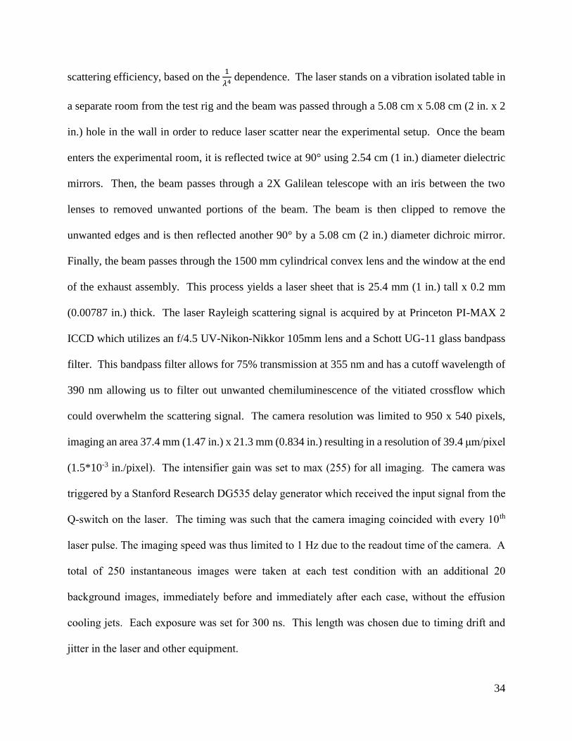
Figure 23: Sample IR image utilizing the bandpass filter to block crossflow emission ............... 38

Figure 24: Model of IR camera calibration setup ......................................................................... 39

Figure 25: IR camera calibration curve and error bounds ............................................................ 40

Figure 26: Filtered and normalized IC (a) and ENDIC (b) laser profiles ..................................... 43

Figure 27: Average pixel intensity in the area shown in Fig. 25 for a full set of test images ...... 43

Figure 28: Raw LRS image (a) and a filtered/corrected image (b)............................................... 44

Figure 29: Normalized shot energy over the course of a single test ............................................. 45

Figure 30: Locations of known temperature, chemistry, and intensity used for calculating

background intensity ..................................................................................................................... 47

Figure 31: Relative Rayleigh scattering cross-section vs temperature and temperature vs relative

detected intensity .......................................................................................................................... 47

Figure 32: Overview of LRS image processing ............................................................................ 48

Figure 33: Sample of individual contributions to temperature calculation uncertainty for air

injection......................................................................................................................................... 49

x

Figure 34: Overall temperature uncertainty (%) as a function of temperature for both air and

CO2 injection ................................................................................................................................. 50

Figure 35: Sample filtered LRS image taken along the centerline of a single row of holes ........ 51

Figure 36: Average LRS temperature images for blowing ratios of 10, 5, and 7 at a height of 2

mm with CO2 coolant, s=4.65 ....................................................................................................... 54

Figure 37: Instantaneous LRS temperature images for blowing ratios of 10, 5, and 7 at a height

of 2 mm with CO2 coolant, s=4.65 ............................................................................................... 54

Figure 38: Average LRS temperature images for blowing ratios of 10, 5, and 7 at a height of 2

mm with air coolant, s=3.05 ......................................................................................................... 55

Figure 39: Instantaneous LRS temperature images for blowing ratios of 10, 5, and 7 at a height

of 2 mm with air coolant, s=3.05 .................................................................................................. 56

Figure 40:Average LRS temperature images for air and CO2 at 3 different heights and a blowing

ratio of 5 ........................................................................................................................................ 57

Figure 41: Instantaneous LRS temperature images for air and CO2 at 3 different heights and a

blowing ratio of 5 .......................................................................................................................... 58

Figure 42: Average and instantaneous LRS temperature images for CO2 injection at 3 mm and

blowing ratio of 5 .......................................................................................................................... 60

Figure 43: RMS deviation from the mean image for CO2 injection at a blowing ratio of 7......... 60

Figure 44: Instantaneous LRS temperature image of CO2 injection at a blowing ratio of 10 and

distance of 3mm from the wall highlighting the individual jet interactions ................................. 60

Figure 45: RMS deviation from the mean image for air injection at a blowing ratio of 7 ........... 61

Figure 46: Microscopic images to two laser drilled holes on the test plate .................................. 62

Figure 47: Repeatability test cases for CO2 injection at a distance of 2.5 mm from the wall ...... 63

Figure 48: Average LRS temperature images for all CO2 cases, s=4.65 ...................................... 71

Figure 49: Sample instantaneous LRS temperature images for all CO2 cases, s=4.65 ................. 72

Figure 50: Average LRS temperature images for all air cases, s=3.05......................................... 73

Figure 51: Sample instantaneous LRS temperature images for all air cases, s=3.05 ................... 74

xi

Abstract

An experimental methodology for studying the mixing and heat transfer characteristics of

effusion cooling jets was developed alongside an experimental test section. Preliminary

investigations into these phenomena were performed in an environment relevant to gas turbine

combustors. An array of effusion jets were injected into a hot vitiated crossflow containing

combustion products at an average temperature of 1500K. Planar images of gas temperature via

Rayleigh scattering were obtained parallel to the injection plane at various heights for two density

ratios (4.65 and 3.05) and three blowing ratios (5, 7, and 10).

The main goal of this data collection was for validation of the methodology and improving

the fundamental understanding of the fluid mechanics involved. The instantaneous gas temperature

distributions reveal that there are significant fluctuations in the motion of the effusion jets which

can be attributed to 3 different sources:

1.) Flow interactions between the individual jets.

2.) Entrainment of the crossflow.

3.) Geometry of the effusion jet hole creating turbulence prior to injection.

It was also observed that for a set blowing ratio, as density ratio decreased, fluctuations in the jet

motion increased. Additionally, jet penetration depth increased with decreasing density ratio.

1

1. Introduction

1.1 Background

As gas turbine technology continues to improve, due to the drive for higher gas turbine cycle

thermodynamic efficiency, combustion chambers are subjected to increasingly high temperatures

and thermal stresses. With current turbine inlet temperatures approaching 2000 K, more

aggressive cooling techniques must be utilized to protect the walls of the combustor as the

combustion gasses are well in excess of the softening temperature of the metallic liner. A

progression of temperature capabilities for turbine and combustor materials can be seen in Fig. 1

with the largest performance increases due to film cooling and TBC (thermal barrier coating)

advances and a projected performance increase due to the implementation of CMC’s (ceramic-

matrix composites)

Figure 1: The progression of temperature limits for Nickel based super alloys utilized in gas turbine engines, as well as the

gas temperature limit with the progression in cooling [1]

2

Film cooling and effusion cooling are often used interchangeably and allows the operating gas

temperature to be higher than the material’s limit. Small amounts of coolant are diverted from the

bypass air and forced through an array of holes to create a cooling gas film over the surface.

Effusion cooling is generally characterized by many small effusion jets emanating from densely

packed, angled, holes creating a full film coverage. This film not only cools the surface of the

combustor liner but also serves as a protective layer preventing turbulent flames from interacting

with the surface [2].

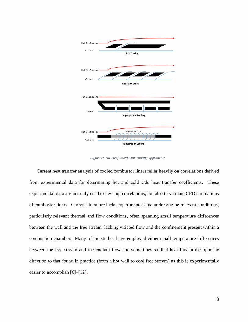
Various types of combustor liner cooling schemes have been extensively researched and some

of these can be seen in Fig. 2. These designs must make efficient use of the coolant air, as drawing

more air from the bypass will reduce the overall thrust specific fuel consumption. The simplest

configuration would be coolant issuing from a slot or single row of holes. However this type of

film generation is not effective in producing a lasting full film coverage, due to instabilities present

in a single jet [3]. It has been shown that around 7 rows of holes are required for full film coverage

to develop, although this number can vary depending on configuration. Transpiration cooling

relies on a porous medium, typically sintered stainless steel with a pore size ranging between 1

and 50 micron and having a wall thickness of about 1 mm [4]. Although transpiration cooling has

been extensively shown to be an efficient cooling method, it has yet to be widely adopted in

combustor design due to manufacturing costs, as well as thermal and mechanical stress constraints.

Impingement cooling was another early approach to this problem, where bypass air impinges onto

the outside walls of the combustor liner, however this method only cools the walls while providing

no protection film from the hot combustion gasses. In recent years, many new variants have been

researched including transply cooling developed by Rolls Royce [5] which utilizes a double walled

combustor liner in which both impingement cooling and effusion cooling are present.

3

Figure 2: Various film/effusion cooling approaches

Current heat transfer analysis of cooled combustor liners relies heavily on correlations derived

from experimental data for determining hot and cold side heat transfer coefficients. These

experimental data are not only used to develop correlations, but also to validate CFD simulations

of combustor liners. Current literature lacks experimental data under engine relevant conditions,

particularly relevant thermal and flow conditions, often spanning small temperature differences

between the wall and the free stream, lacking vitiated flow and the confinement present within a

combustion chamber. Many of the studies have employed either small temperature differences

between the free stream and the coolant flow and sometimes studied heat flux in the opposite

direction to that found in practice (from a hot wall to cool free stream) as this is experimentally

easier to accomplish [6]–[12].

4

In order to continue the evolution of effusion cooled combustor liners, experimental data

regarding heat transfer, flow structure, and flow interaction at engine relevant thermal and flow

conditions is needed not only to validate models, but also to develop a better understanding of the

problem at hand. In the following, past and current research on effusion cooling technology is

reviewed and the rationale for my research is highlighted.

1.2 Previous Effusion Cooling Studies

Understanding the interaction between the primary flow and secondary effusion flow has

been a topic of great interest among researchers for the past several decades as it has direct

relevance to gas turbine combustors. The work done by Mayle & Camarata [9], Papell [13],

Metzger et al. [2], and Choe et al. [14] laid the groundwork for current research by developing the

standard practice for research regarding effusion cooling. This research sought to better

understand and quantify the effect of varying hole arrangement, hole spacing, injection angle,

blowing ratio, and density ratio on cooling effectiveness and the heat transfer from the bulk flow

to the combustor liner. Blowing ratio is defined as

𝐵𝑅 =𝜌𝑗𝑢𝑗

𝜌𝑐𝑓𝑢𝑐𝑓 (1.1)

where 𝜌 is density, 𝑢 is velocity, and the subscripts 𝑗 and 𝑐𝑓 refer to the effusion jets and crossflow

respectively. Density ratio is defined as:

𝑠 =𝜌𝑗

𝜌𝑐𝑓 (1.2)

Cooling effectiveness is defined as:

5

𝜂 =𝑇ℎ−𝑇𝑤

𝑇ℎ−𝑇𝑐 (1.3)

where 𝑇ℎ is the bulk crossflow temperature, 𝑇𝑤 is the adiabatic wall temperature, and 𝑇𝑐 is the

coolant injection temperature. The ultimate goal of this research was to identify which

configurations of these parameters optimized cooling effectiveness in order to maximize

combustor durability under hostile conditions.

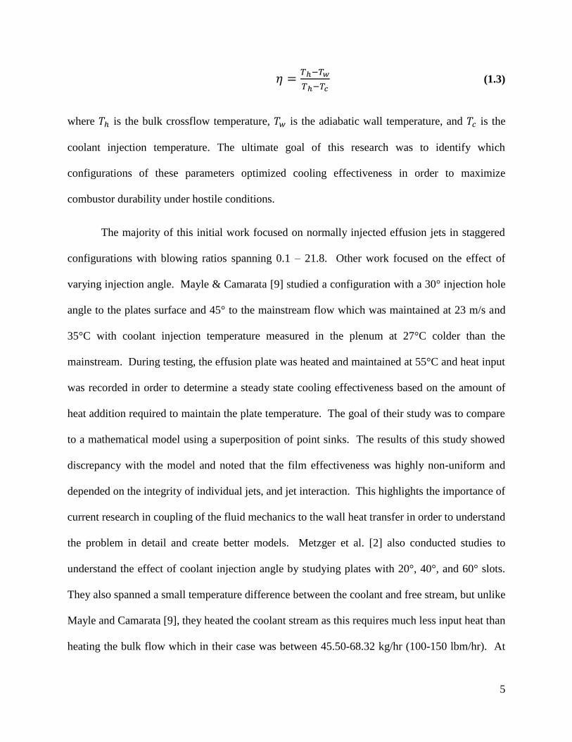
The majority of this initial work focused on normally injected effusion jets in staggered

configurations with blowing ratios spanning 0.1 – 21.8. Other work focused on the effect of

varying injection angle. Mayle & Camarata [9] studied a configuration with a 30° injection hole

angle to the plates surface and 45° to the mainstream flow which was maintained at 23 m/s and

35°C with coolant injection temperature measured in the plenum at 27°C colder than the

mainstream. During testing, the effusion plate was heated and maintained at 55°C and heat input

was recorded in order to determine a steady state cooling effectiveness based on the amount of

heat addition required to maintain the plate temperature. The goal of their study was to compare

to a mathematical model using a superposition of point sinks. The results of this study showed

discrepancy with the model and noted that the film effectiveness was highly non-uniform and

depended on the integrity of individual jets, and jet interaction. This highlights the importance of

current research in coupling of the fluid mechanics to the wall heat transfer in order to understand

the problem in detail and create better models. Metzger et al. [2] also conducted studies to

understand the effect of coolant injection angle by studying plates with 20°, 40°, and 60° slots.

They also spanned a small temperature difference between the coolant and free stream, but unlike

Mayle and Camarata [9], they heated the coolant stream as this requires much less input heat than

heating the bulk flow which in their case was between 45.50-68.32 kg/hr (100-150 lbm/hr). At

6

the conclusion of the study, empirical correlations were developed for the cooling effectiveness

but they only hold for a small range of the tested parameters. Furthermore, the interaction between

the coolant and bulk flow could have been affected by the direction of heat flux in their experiment.

The formation of the turbulent boundary layer and its characteristics are directly affected by the

direction of the heat flux, and with the lengths scales of the effusion films being small, this

turbulence could have a direct effect on heat transfer properties. Papell [13] focused on

investigating the effects of coolant injection angle while working for NASA in 1960’s. The goal

of his study was also to develop empirical correlations for the film cooling effectiveness as a

function of slot angle with the focus on fluid discharge angles of 45°, 80°, and 90°. For his

experiment, the bulk flow temperature was maintained at 833K (1500 °R) and coolant temperature

was varied. He, like the other mentioned previously, developed empirical correlations for cooling

effectiveness under a specific range of parameters.

For all of these early studies, embedded thermocouples were used to record temperatures,

which were used to determine heat transfer coefficients and cooling effectiveness. However, this

only allowed for a vague understanding of a time averaged result at discrete locations within the

plate at temperatures and geometries largely unrealistic for gas turbine combustors. The results of

these studies matched poorly with analytical models and relied on empirical models in order to

calculate cooling effectiveness which only hold for small ranges of parameters. Understanding

the instantaneous interactions between the bulk flow, coolant, and individual jets is still something

that the community is working to improve.

Continuing from these initial studies more effort was focused on developing experimental

methods in order to better understand how the main test parameters affect cooling effectiveness

and heat transfer characteristics. However, lack of combustor relevant operating conditions, and

7

comprehensive data collection has rendered a majority of this work as preliminary. Due to the

difficulty of performing experiments at relevant operating conditions, particularly thermal

conditions relevant to combustors, numerical techniques have been employed to gain further

insight regarding heat interaction between the flow and combustor liner. Miller & Crawford [15]

were one of the first groups to publish a strictly numerical study about implementing a numerical

strategy to investigate multiple rows of cooling holes for a wide variety of geometries. They

utilized a modified version of STANCOOL, which is a two-dimension boundary layer program,

to simulate the film cooling process of discrete hole injection with turbulence augmentation.

However, this model did not utilize full Navier-Stokes calculations, and had to be tuned in order

to fit experimental data within a set range of parameters. While this was a large step in the right

direction, it still required experimental data in order to create the model and could not be used

outside of the experimental parameter range.

Work from Liu et al. [16] and others used numerical techniques to demonstrate the heat

transfer superiority of effusion cooling over the traditional slot cooling by building upon previous

numerical work. Bohn & Mortiz [17], Andreini et al. [18], and Hu & Ji [19] worked to expand the

parameter range of numerical simulations by studying hole shape, spacing, and angle dependence

on effusion cooling and overall film coverage. Nevertheless, the majority of mathematical models

were created using combustor relevant conditions and have to be validated using experimental

results at combustor relevant conditions before widespread use and implementation.

In more recent literature, more advanced diagnostic techniques were utilized for

determining both heat and mass transfer properties, and characterizing the flow interactions of

effusion jets. Planar laser-induced fluorescence (PLIF) and infrared (IR) imaging have assisted

researchers to develop better qualitative and quantitative understanding of effusion jet interactions.

8

Fric et al. [20] utilized planar laser-induced fluorescence to quantify fluorescein dye concentrations

within a water tunnel in order to quantify mixing characteristics. The study focused on full

coverage, discrete hole film cooling, specifically geometries applicable to gas turbine combustor

liners. The cooling holes had an injection angle of 20° with holes diameters of 2.54 mm and 0.61

mm. Blowing ratios in the range of 0.5-5.7 were studied and diagnostics were performed as close

as 0.25 mm from the wall. The results of the experiment showed that blowing ratios in the range

of 1.7-3.3 were least effective at creating full film coverage, while blowing ratios less than 1.7 or

greater than 3.3 had improved film coverage. It was also shown that jet separation behavior and

coalescence were both functions of blowing ratio. While this was a great step forward in terms of

understanding the fluid flow interactions, the authors do recognize the limitations of studying

effusion jets in a water tunnel, specifically the lack of large density differences between the cooling

stream and crossflow.

McGhee [21] and Shrager & Thole [8] have heavily relied on the use of infrared

thermography to determine surface temperature when cooling jets are injected into a heated

primary flow. This is a drastic improvement to prior research which relied on embedded

thermocouples and allows for improved spatial resolution of cooling effectiveness, but lacks any

experiments studying of the fluid flow interactions. Facchini et al. [11] utilized a characterized

thermochromic liquid crystal (TLC) paint inside of their test section in order to determine

temperature. This paint changes properties with temperature and therefore images from a digital

camera under known conditions can be converted into temperature maps with a high degree of

accuracy. Their experimental results were then utilized to validate their in-house numerical

simulation. However, the model was not able to make a realistic prediction of experimental results

and drastically under predicted cooling effectiveness values. Andreini et al. [12] continued the

9

work of Facchini by expanding experimental parameters. The results of this study suggest the

velocity ratio is the driving parameter for heat transfer phenomena. Along with this, they state that

the effects of density ratio can be neglected within the penetration regime. When velocity ratio

was held constant, it was also found that cooling effectiveness increased with increasing density

ratio.

While all of this work has been moving in the right direction, there is still a large disconnect

between the fluid dynamics and heat transfer characteristics, as none of the work discussed studied

both the fluid flow interaction and the heat transfer simultaneously. The work presented in this

thesis is an attempt to connect the heat and fluid phenomena by studying both gas phase and surface

temperatures of effusion jets within a hot (1500K bulk flow), vitiated flow in a relevant combustor

geometry. This allows for a more holistic understanding and characterization of effusion jet

interaction while still determining cooling effectiveness with high special resolution.

2. Theoretical Basis of Methodology

2.1 Laser Rayleigh Scattering

Laser Rayleigh scattering is a diagnostic often utilized for studying the dynamics and

interactions of gas flows. Since it is a non-intrusive optical diagnostic technique, it has a wide

array of applications and has been used by many researchers to take almost instantaneous

snapshots of gas properties. Laser Rayleigh scattering was utilized by Sutton [22] and Arndt et

al[23]. to determine density, Feikema et al. [24], Barlow et al. [25], and Balla et al. [26] to

determine mixture fraction, along with Gordon et al. [27] and Barat et al. [28] to determine

temperature. It is possible to perform this diagnostic in both reacting and non-reacting flows and

it has many useful properties. For the current work, laser Rayleigh scattering was utilized to

10

determine gas temperatures. The theory behind the current use of laser Rayleigh scattering is

reviewed in the following section.

2.1.1 Rayleigh Scattering Cross-Section

Rayleigh scattering was originally investigated by Lord Rayleigh, Jean Cabannas and others in the

19th century as a means for understanding the intensity, color, and polarization of light within the

atmosphere. Rayleigh scattering is the phenomena in which light is scattered from particles whose

diameters are much smaller than the wavelength of incident light. In the case of Lord Rayleigh’s

work, the incident light was broadband, and un-polarized, originating from the sun. By studying

the color, and intensity of the light scattered by the earth’s atmosphere, Lord Rayleigh concluded

that the scattering intensity of air molecules is inversely proportional to the incident light

wavelength to the fourth power and is also dependent on the number of particles excited by the

incident light [29]. Laser Rayleigh scattering utilizes a single wavelength light source and does

not need large volume integration such as Lord Rayleigh used, however his research is still highly

relevant

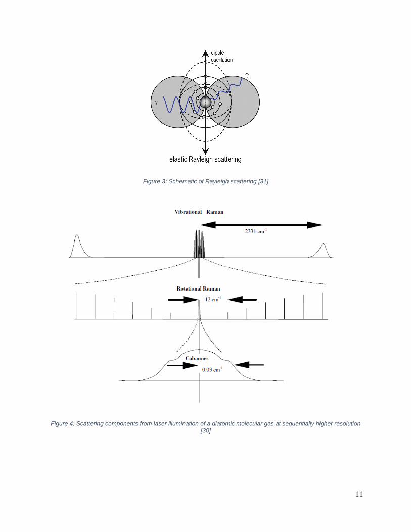
In 2001, Miles et al. [30] reviewed the use of Rayleigh scattering in diagnostics, and

showed the use of multiple methods for deriving scattered light intensity by treating the scatted

light as radiation from and infinitesimally small oscillating dipole and the use of the differential

Rayleigh scattering cross-section. A diagram of this oscillating dipole is show in Fig. 3 [31]. When

using lasers as the incident light source, the Rayleigh signal is the summation of the coherent

Cabannas lines, the rotation Raman lines and the vibrational Raman lines as seen in Fig. 4 [30].

11

Figure 3: Schematic of Rayleigh scattering [31]

Figure 4: Scattering components from laser illumination of a diatomic molecular gas at sequentially higher resolution [30]

12

Expressions for total scattering cross section 𝜎 (cm2) and differential scattering cross

section for linearly, vertically polarized incident light 𝜕𝑉𝜎0

𝜕 Ω (cm2 sr-1), were derived including all

components and are defined as:

𝜎 =32𝜋2(𝑛−1)2

3𝑁2𝜆4 (6+3ρ0

6−7𝜌0) (2.1)

𝜕𝑉𝜎0

𝜕 Ω=

3𝜎

8𝜋 (

2

2+𝜌0) (2.2)

where 𝑛 is the gas index of refraction, 𝑁 is the number density of scatterers (cm-3), 𝜆 is the incident

laser wavelength (cm) and 𝜌0 is the depolarization ratio of polarized light. In laser applications,

the light output is polarized and therefore the depolarization ratio and linearly polarized incident

light must be utilized in finding the differential scattering cross-section. Long’s [32] expressions

for the un-polarized and linearly polarized depolarization ratios (𝜌0 and 𝜌) are:

𝜌0 =6𝛾2

45𝑎2+7𝛾2 (2.3)

𝜌 =3𝛾2

45𝑎2+4𝛾2 (2.4)

where 𝛾2 and 𝑎2 are the traditional invariants in the anisotropy and mean polarizability tensor

respectively. By rearranging Eq. (2.4) to solve for 45𝑎2, substituting into Eq. (2.3), and

simplifying, one can find an expression for the depolarization ratio of un-polarized light in terms

of the depolarization ratio of linearly polarized light:

𝜌0 =2𝜌

1+𝜌 (2.5)

13

By substituting Eqs. (2.1) and (2.5) into Eq. (2.2), one can derive the expression for total

differential Rayleigh scattering cross-section for vertically polarized incident light that is used in

the current work:

𝜕𝜎

𝜕 Ω=

4𝜋2(𝑛−1)2

𝑁2𝜆4 (6+6𝜌

6−8𝜌) (2.6)

2.1.2 Rayleigh Thermometry

For the application of laser Rayleigh scattering, the power of the signal collected, 𝑃𝐷 (W),

is dependent on the integral of the effective differential Rayleigh scattering cross-section over the

collection angle, ΔΩ (sr), the number density of scattering particles, 𝑁 (mol cm-3), the probe

volume, 𝑉 (cm-3), the incident laser intensity, 𝐼𝐿 (W cm-2), and the efficiency of all collection

optics, 𝜂 [30]:

𝑃𝐷 = 𝜂𝐼𝐿𝑁𝑉 ∫ (𝜕𝜎

𝜕 Ω)

𝑒𝑓𝑓𝜕Ω

ΔΩ (2.7)

For the majority of laser diagnostic applications and in the case of the current work, Rayleigh

scattered light is detected by a collection lens over a small collection angle with which Eq. (2.7)

can be approximated as [22]:

𝐼𝐷 = 𝜂𝐼𝐿𝑛𝑙Ω (𝜕𝜎

𝜕 Ω)

𝑒𝑓𝑓 (2.8)

where the detected signal intensity, 𝐼𝐷 (W cm-2), is dependent on the concentration of scattering

gas molecules in the probe volume 𝑛 (number*cm-3), the length of the probe volume on the

detector, 𝑙 (cm), the solid angle of the collection optics, Ω (sr), and the effective Rayleigh scattering

cross-section of the scattering molecules, (𝜕𝜎

𝜕 Ω)

𝑒𝑓𝑓 (cm2 sr-1). In the situation where the scattering

14

gas consists of multiple molecules, such as air, the effective differential Rayleigh scattering cross-

section is the molar averaged value of all molecules:

(𝜕𝜎

𝜕 Ω)

𝑒𝑓𝑓= ∑ 𝑋𝑖 (

𝜕𝜎

𝜕 Ω)

𝑖, 𝑖 = 1,2,3 … , 𝐾 𝐾

𝑖=1 (2.9)

where 𝑋𝑖 and (𝜕𝜎

𝜕 Ω)

𝑖 are the mole fraction and corresponding differential Rayleigh scattering cross-

section of the i-th molecule, and 𝐾 is the total number of molecules in the mixture.

When using laser Rayleigh scattering to perform diagnostics in a gaseous mixture, and total

pressure is known, the concentration of molecules within the probe volume can be related to the

temperature by the ideal gas law:

𝑛 =𝑝𝑁𝐴

𝑅𝑇 (2.10)

where 𝑝 (atm) is the gas pressure, 𝑁𝐴 (6.022 x 1023 mol-1) is Avogadro’s number, 𝑅 (82.057 cm3

atm K-1 mol-1) is the universal gas constant, and 𝑇 (K) is the gas temperature. When using this

correlation in laser Rayleigh scattering, the diagnostic is typically referred to as Rayleigh

thermometry. In experiments, a photodetector is normally used to measure the energy of the

incident laser pulse, 𝐸𝑝 (mJ), and this is related to laser intensity by:

𝐸𝑝 = ∫ 𝐼𝐿𝐴𝑑𝑡 = 𝐼𝐿𝐴Δ𝑡 =𝐼𝐿𝐴

𝑓𝑝Δ𝑡 (2.11)

where 𝐴 (cm2) is the area of the laser beam, and 𝑓𝑝 (Hz) is the frequency of the laser pulse. By

substituting Eqs. (2.9), (2.10), and (2.11) in Eq. (2.8), one finds the laser Rayleigh scattering signal

for Rayleigh thermometry to be:

15

𝐼𝐷 =𝜂𝑓𝑝𝑝𝑁𝐴𝑙Ω

𝐴𝑅

𝐸𝑝

𝑇 ∑ 𝑋𝑖 (

𝜕𝜎

𝜕 Ω)

𝑖, 𝑖 = 1,2,3 … , 𝐾 𝐾

𝑖=1 (2.12)

For most applications, Eq. (2.12) is simplified to:

𝐼𝐷 = 𝐶𝐸𝑃

𝑇∑ 𝑋𝑖 (

𝜕𝜎

𝜕 Ω)

𝑖, 𝑖 = 1,2,3 … , 𝐾 𝐾

𝑖=1 (2.13)

where 𝐶 is an experimental constant that includes all of the constants related to experimental setup

as:

𝐶 =𝜂𝑓𝑝𝑝𝑁𝐴𝑙Ω

𝐴𝑅 (2.14)

and is often referred to as a calibration constant. By rearranging Eq. (2.13) the final expression

for the gas temperature is determined for the application of non-intrusive Rayleigh thermometry:

𝑇 = 𝐶𝐸𝑃

𝐼𝐷∑ 𝑋𝑖 (

𝜕𝜎

𝜕 Ω)

𝑖, 𝑖 = 1,2,3 … , 𝐾 𝐾

𝑖=1 (2.15)

2.2 Infrared Thermography

In this study infrared thermometry was planned to be utilized to characterize temperature

field of the surfaces of the effusion plates. In this section, the important theoretical aspects to be

considered when utilizing infrared sensors to detect surface temperatures of an object are presented

and discussed. While the utilization of IR cameras has become prevalent within the research

community, one must take caution to account for significant variations in radiative signal due to

the environment. This is particularly important in IR imaging in combusting flows where

interferences from gas emission and absorption can affect the measurements.

16

2.2.1 Infrared Radiation

All objects and molecules are constantly emitting electromagnetic radiation due to their

internal energy. Figure 5 shows black body emission at different temperatures given by Planck

distribution, where a blackbody is a perfect radiative emitter with an emissivity value of one.

Figure 5: Blackbody radiation curves [33]

Planck’s law of black-body radiation is given by:

𝐸𝜆.𝑏(𝜆, 𝑇) =2𝜋ℎ𝑐2

𝜆5

1

𝑒ℎ𝑐

𝑘𝑇𝜆−1

(2.16)

17

where 𝐸𝜆.𝑏 is the spectral blackbody emissive power, ℎ is Planck’s constant, c is the speed of light

in a vacuum, k is the Boltzmann constant, 𝜆 is the wavelength of the radiation, and T is the absolute

temperature of the body. The integration of this curve to attain the total radiative emission yields:

𝐸 =4𝜎

𝑐𝑇4 (2.17)

where E is energy density (total energy per unit volume) and 𝜎 is the Stan-Boltzmann constant.

Thermal radiation in the range of 0.1 to 1000 𝜇𝑚 includes both visible and infrared

wavelengths, but infrared imaging sensors typically detect radiation in the range of 3 to 5 𝜇𝑚 or 7

to 14 𝜇𝑚. Some sensors also have to ability to select the band being imaged typically in the range

from 3 to 14 𝜇𝑚 [21] for temperatures ranging from 250K – 1500K. The intensities and

corresponding wavelengths of radiation emitted by an object depend upon its surface properties,

as well as its temperature. Since radiation is transferred to and from all objects in an environment,

one must take precaution to minimize reflections from other radiation sources as it can impact the

detected signal on the sensor and cause errors in the collected data. Along with this, if the imaging

is performed in a test enclosure, proper window material selection is important as many types of

glass do not transmit IR signal efficiently.

2.2.2 Infrared Detectors

The first studies involving the use of infrared sensors to measure temperature utilized single

element detectors which allowed for instantaneous temperature readings in a non-intrusive

manner. These detectors were typically translated across an area of interest (at steady state

temperatures) to create 1-D and 2-D temperature distributions of a surface. Modern sensors utilize

18

multi-element detector arrays which can output 2-D temperature maps without translation.

However, with this comes a tradeoff. By utilizing a single sensor, each location has a fixed

measurement error. With an array, each sensor has a small amount of variability between elements,

which is specific to an individual camera, which means that at each location, there can be a slight

difference in measurement error. This variation in sensors is often compensated in modern IR

cameras by utilizing an internal blackbody source to calibrate each sensor and reduce the

variability. In the case of the work presented here, an “in-situ” calibration was performed to

account the effects of sensor element variability.

Similar to visible light captured by optical cameras, infrared cameras focus the incoming

radiation onto a focal plane sensor array where each sensor element (or pixel) detects the

electromagnetic radiation and converts it first into an analog voltage output, and then digitizes it

to “counts”. Many modern cameras utilize software which automatically converts these counts

into temperature based on factory calibrations and user provided surface properties like emissivity.

In order to maintain accurate signal conversion, the sensors must be cooled and kept at a constant

temperature, otherwise the measured signal will drift as the sensor array heats up. Early models

utilized liquid nitrogen for cooling, but the current industry norm is thermo-electric cooling of IR

imaging cameras [21]. The camera being used for the current work (FLIR SC6700) maintains the

sensor temperature at ~74K during operation.

19

2.2.3 Radiative Properties

2.2.3.1 Surfaces

Unlike the black-body curves shown in Fig. 5, most real surfaces do not emit a smooth

continuous curve of spectral radiation, and it often has large spikes or dips due to the surface and

material properties. Seen in Fig. 6 is a visual example of the difference between emission from a

real surface (gray-body) and a blackbody [33]. These differences are caused by the emissivity (𝜖)

of the object being a function of the wavelength of radiation, where the emissivity is variable with

wavelength and temperature for most materials. [34]. Figure 7 shows the emissivity of n-type

phosphorous-doped silica (n-Si) as a function of wavelength and temperature as an example.

Figure 6: Visual comparison of radiation from a blackbody and a real surface[33]

20

Figure 7: Emissivity of n-Si as a function of wavelength [34]

Due to the variation of material surface emissivity, it is important to know the material

properties when one is using an infrared camera or sensor in to measure surface temperature.

Without this knowledge, or an accurate in-situ calibration, precise measurements of surface

temperature would not be possible. Many times, the software provided with an IR camera allows

a user to specify the emissivity, however most of the time this sets a constant value, as the camera

detects radiation in a range of wavelengths and is not able to account for emissivity variation within

that range. It simply collects radiation intensity in the designed wavelength range. Therefore, if

the material being imaged has an emissivity which varies drastically within the detection range, a

user calibration based on raw image “counts” may be better suited than utilizing the manufacturers

calibration. Temperature dependence of emissivity, which is indirectly connected with its spectral

variation, can also present issues for IR temperature imaging.

21

2.2.3.2 Viewing Windows

If an experiment requires a closed vessel as is the case in the work presented here, then the

choice of material for a viewing window is very important as radiation from the source needs to

be transmitted to the camera. Various types of scientific glass are used in laboratories but most

are not suitable for IR imaging. This is due to a few different properties which include reflectivity,

emissivity, and transmittance.

Historically, the glasses used for windows in our experimental combustion rig are either

fused quartz, or UV-fused silica, which resist thermal shock, allow optical access for laser

diagnostics, and are relatively inexpensive. These two types of glass however, have very poor

transmission in the IR region. The transmission spectrum from the manufacturer for fused quartz

used in our lab is shown in Fig.7 and an example transmission spectrum for UV-Fused Silica is

shown in Fig. 8. The detection range of 3 - 5 𝜇𝑚 is highlighted.

Figure 8: Transmission spectra for fused quartz [35]

22

Figure 9: Transmission spectra for UV-fused silica [36]

From these figures, it is clear that neither of these materials have a significant amount of

signal transmission in the wavelength detection range of the camera being used (3-5𝜇m). While

there is some signal transmission in this range, if imaging were performed through these materials,

there would be a very low signal to noise ratio (SNR), which creates a high degree of uncertainty

in the measured temperatures. Along with this, both of these materials have a high reflectivity in

the camera detection range, meaning that objects near the window, or within its view, can have

radiation reflected off the window onto the sensor which again increases the error in the

measurement. An ideal window would have minimal reflectivity and high transmission in the

detection range.

Another important factor to consider is the emissivity of the glass itself if the glass is at a

significantly high temperature as in a combustion experiment. The radiation emitted from the hot

glass can impact or even overwhelm the radiation from the source whose temperature is being

measured. It is important that the glass has little to no emission in the wavelength range being

detected. Shown in Fig. 10 is the emittance of fused quartz as a function of wavelength [37], which

shows that there is significant emission within the desired range at high temperature. Thus, quartz

is not a good choice for IR imaging since it has low transmittivity in the wavelength detection

23

range; emitted radiation from the hot window overpowers the small amount of radiation

transmitted through the window from the surface to be measured.

Figure 10: Emissivity of fused quartz at 785K [37]

Knowing that the ideal window must have high transmission, low reflectivity, and low

emissivity in the detection range, one can find a suitable material for imaging through. In the work

discussed here, a sapphire window was chosen. Shown in Fig. 11 are the radiative properties of

sapphire as investigated by Babladi [37]. Sapphire has a low reflectance, and high transmission

within the range of interest, but has a non- insignificant amount of emission for wavelengths

greater than 4.16 micron. The emission in this regime will not affect the measurements taken in

the specific instance of the work being presented here because a bandpass filter (3.85-4.05 𝜇m,

2469-2597 cm-1) was implemented for other reasons which will be discussed in Section 3.5.1.

24

Figure 11: Radiative properties of sapphire: reflectance, transmittance, and emittance [37]

25

2.2.3.3 Viewing Surface Radiation Through Combustion Gas Medium

One other factor that should be considered but does not always have a significant effect is

the properties of the medium through which IR imaging of a surface is being performed. This will

be discussed more in depth and related to the current work in Section 3.5.1, but a brief discussion

is included here.

Gasses just like surfaces, can absorb and emit spectral radiation. Typically, the intensity

of this absorption or emission is low, but over large optical thicknesses and in strongly participating

gas environments, this can create an issue. Over short distances (less than 1 meter), the absorption

of a typical atmosphere can be neglected as it is infinitesimal, but over large distances or in high

pressure situations, the absorption of the incident radiation increases and can impact acquired data

if not accounted for. An example of absorption in earth’s atmosphere [38] is shown in Fig. 12. In

imaging through combustion gasses, CO2 and H2O emit and absorb significant amounts of

radiation in the IR spectrum at high temperatures. If possible, one should choose a wavelength

range to investigate which does not contain emission from these gasses, however that may not

always be possible.

Figure 12: Transmission of earth's atmosphere [38]

26

3. Experimental Methodology

This section covers the experimental design of the test rig and the data acquisition system.

3.1 Experimental Test Rig

.

The experimental test rig consisting of 4 main sections: the preburner, transition section,

test section, and the exhaust is shown in Fig. 13. Another high-level schematic of the rig is shown

in Fig. 14 with the dimensions of each section.

Figure 13: High level model view of the experimental test rig

The pilot flame generates the vitiated gas flow by utilizing a swirl type burner to combust

a premixed propane air mixture with an equivalence ratio (𝜙) of 0.865. This burner is same as the

one described by Wagner et al. [39] used in jet-in-crossflow studies. This burner is ignited by a

premixed propane air torch labeled as “igniter” in Fig. 14. This igniter flame is deactivated once

the pilot flame is burning stably. This pilot flame does not extend into the test section and is

confined within the transition section.

27

Figure 14: High-level schematic of the experimental test rig

The transition section is manufactured with a stainless-steel outer shell and lined with a

3.81 cm (1.5 inches) thick layer of Kast-O-Lite 97L refractory in order to reduce heat losses and

protect the outer stainless-steel casing during long run times. The transition section has an initial

circular cross section with a diameter of 11.18 cm (4.4 in.) and converges to a final cross section,

matching that of the test section, of 3.81 cm x 7.62 cm (1.5 in. x 3 in.) This transition follows a

5th order contraction developed by Bell & Mehta [40] in order to produce a “top hat” velocity

profile. The casting process of the transition section involved centering a PVC tube and a 3-D

printed transition shape insert in the outer stainless-steel shell and pouring the Kast-O-Lite around

this core which provided a smooth inner wall to the transition section after following the

manufacturer’s curing process. The outside of the transition section was wrapped in 15.24 cm (6

in.) of ceramic insulation to further reduce heat loss in this section. The length of the transition

section as described in [41], was chosen so that the pilot flame did not extend into the test section.

The test section can be seen in a high-level view in Fig. 15 and a more detailed view in Fig.

16. The inner dimensions are 3.81 cm (1.5 in.) in height and 7.62 cm (3 in.) in width chosen as

28

the relevant size scale for effusion cooling studies. The test section is made out of stainless-steel

and has walls which are 1.78 cm (0.7 in.) thick. Each wall contains an embedded K-type

thermocouple utilized for radiation correcting the flow temperature measurements.

Figure 15: High level model view and flow paths of the test section

Figure 16: Detailed schematic of the test section

The test section features 3-sided optical access, with each wall having the ability to

accommodate either a window (quartz for Rayleigh imaging and sapphire for IR imaging), or a

stainless-steel blank if optical access on that wall is not desired. The window dimensions are 15.24

29

cm x 4.58 cm (6 in. x 1.8 in.) for the side walls and 15.24 cm x 6.35 cm (6 in. x 2.5 in.) for the top

wall with both being 6 mm (0.236 in.) in thickness. Both the windows and blanks are held in place

by a 1.1 mm (0.03 in.) flange in the test section and compression flange bolted above as shown in

Figs. 15 and 16. Included in the design is the provision to install a window on the backside of the

plenum for IR imaging of the backside of the effusion plate. These windows are all sealed in place

using 0.8 mm (1/32 in.) thick graphite seals. The plenum provides the effusion cooling gas to the

test section with the flow rates being controlled by MKS mass flow controllers prior to entry into

the plenum. For the work discussed here, both CO2 and air were utilized as coolant gasses.

The effusion test plate geometry being investigated in this work is shown in Fig. 17. It

features 2 rows of staggered holes with hole spacing of 6.35 mm (0.25 in.) and row spacing of 7.62

mm (0.30 in.) with a total of 20 holes laser drilled at a 30-degree forward angle from the surface.

The thickness of the test plate was 2.29 mm (0.090 in.) and the material in Inconel 625. The

definition here for a row of holes is a set of staggered jets, however the definition of a row varies

in literature. The 6.35 mm (¼ in.) jet downstream of the holes is used for anchoring the gas

temperature measurements as a temperature calibration location and will be discussed in Section

4. The anchoring jet flowrate is separately controlled from the effusion jet flows by means of an

MKS mass flow controller and had a fixed flowrate for all experiments (1.51m/s for air and 1.10

m/s for CO2, Reynolds numbers of 513 and 683 respectively). This test plate was welded into a

stainless-steel blank such that it was flush with the inner side of the test section and this blank is

then bolted onto the bottom of the rig between the plenum and the test section utilizing 0.8 mm

(1/32 in.) graphite seals in between each component. All flow lines supplying the gasses to the

preburner, and coolant for the effusion jets were both leak checked and flow rates were checked

to ensure the flow capability range

30

Figure 17: Effusion test plate geometry

This new test section implements a few design changes from the previous iteration

described in [39], [41], [42]. With the implementation of interchangeable parts, larger optical

access windows, non-machined windows, and other minor changes, this test section is very

versatile in the types of experiments it can accommodate. By allowing for the use of rectangular

windows instead of windows with a machined step as earlier designs employed, manufacturing

cost and time to acquisition of quartz window parts is drastically reduced.

3.2 Crossflow Characterization

High-speed PIV was not performed during the course of this work, however it was

performed in the previous studies several times with good repeatability [41]. The velocity profile

was used to characterize the current work as the test rig components were identical to the earlier

studies. The only differences from the previous test section were the window installation method

and coolant injection section below the test section with all other features being the same. The

velocity profile shown in Fig. 18 is at the same conditions as the current work. Temperature

profiles were measured with an R-type bare bead thermocouple (bead diameter of 0.60 mm) as

shown in Fig. 19. One thing to note is that the temperature values can change slightly from day to

31

day depending on the atmospheric and lab conditions as the compressor draws in air from the

atmosphere to be use in the premixture for the pilot flame. This means that during colder periods

such as winter, the crossflow runs slightly colder than nominal, but it is monitored throughout

testing so this does not affect data analysis. The gas temperature profile was measured by

traversing a bare wire R-type thermocouple (bead diameter of 0.60 mm) across the test section

height at the operating condition by time averaging each data point over several seconds until the

measurement at the location stabilized. The thermocouple was then traversed back and the two

sets of measurements were averaged. This thermocouple temperature data was then radiation

corrected utilizing the test section wall temperature measurements.

Figure 18: Velocity and thermal profiles of the crossflow along the centerline of the test section

The chemical composition of the crossflow was determined by utilizing a computational

model developed in CANTERA within MATLAB [41], [43]. Thermodynamic, transport, and

chemical kinetics data was from the USC-II mechanism [44] were used in the modeling. The

crossflow was modeled in two sections, a 1-D burner-stabilized flame to represent the swirl burner

and a constant pressure reactor system with heat loss, representing the transition section. A

premixed propane-air mixture at standard temperature and pressure (STP), P=1atm, T=300K, with

φ = 0.865 was injected into the burner-stabilized flame (BSF). The combustion products from this

burner were then passed into a reactor system consisting of a constant pressure reactor (CPR) with

32

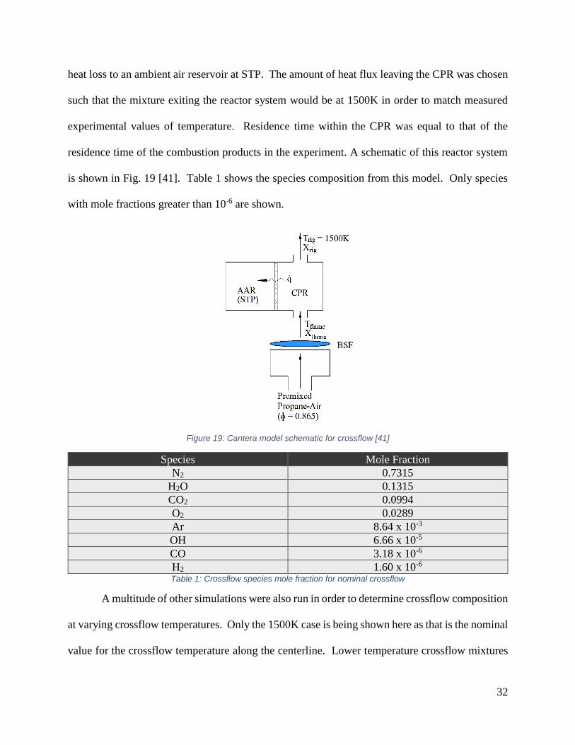
heat loss to an ambient air reservoir at STP. The amount of heat flux leaving the CPR was chosen

such that the mixture exiting the reactor system would be at 1500K in order to match measured

experimental values of temperature. Residence time within the CPR was equal to that of the

residence time of the combustion products in the experiment. A schematic of this reactor system

is shown in Fig. 19 [41]. Table 1 shows the species composition from this model. Only species

with mole fractions greater than 10-6 are shown.

Figure 19: Cantera model schematic for crossflow [41]

Species Mole Fraction

N2 0.7315

H2O 0.1315

CO2 0.0994

O2 0.0289

Ar 8.64 x 10-3

OH 6.66 x 10-5

CO 3.18 x 10-6

H2 1.60 x 10-6

Table 1: Crossflow species mole fraction for nominal crossflow

A multitude of other simulations were also run in order to determine crossflow composition

at varying crossflow temperatures. Only the 1500K case is being shown here as that is the nominal

value for the crossflow temperature along the centerline. Lower temperature crossflow mixtures

33

are necessary for performing laser Rayleigh scattering data analysis near the wall where the

crossflow is colder (1200-1300K). Increasing the amount of heat loss in the constant pressure

reactor does not have a significant effect on the mixture composition however it does affect the

density of the mixture. When calculating the blowing and density ratios of the effusion jets, the

nominal, bulk crossflow characterization was utilized. Utilizing this mixture composition, along

with the hydraulic diameter of the test section, the Reynolds number for this flow was calculated

as 𝑅𝑒𝑐𝑓 = 1610.

3.4 Laser Rayleigh Imaging

3.4.1 Laser and Optical Setup

Shown in Fig. 20 is the laser and optical setup for performing the laser Rayleigh

scattering (LRS) diagnostic.

Figure 20: Laser and optics setup for LRS imaging

The incident light source used for Rayleigh scattering in the current work was a frequency

tripled, 355 nm output laser beam of a Spectra-Physics-Pro-230 Nd YAG with an average pulse

energy of 350 mJ and a repetition rate of 10 Hz. The third harmonic was chosen for maximum

34

scattering efficiency, based on the 1

𝜆4 dependence. The laser stands on a vibration isolated table in

a separate room from the test rig and the beam was passed through a 5.08 cm x 5.08 cm (2 in. x 2

in.) hole in the wall in order to reduce laser scatter near the experimental setup. Once the beam

enters the experimental room, it is reflected twice at 90° using 2.54 cm (1 in.) diameter dielectric

mirrors. Then, the beam passes through a 2X Galilean telescope with an iris between the two

lenses to removed unwanted portions of the beam. The beam is then clipped to remove the

unwanted edges and is then reflected another 90° by a 5.08 cm (2 in.) diameter dichroic mirror.

Finally, the beam passes through the 1500 mm cylindrical convex lens and the window at the end

of the exhaust assembly. This process yields a laser sheet that is 25.4 mm (1 in.) tall x 0.2 mm

(0.00787 in.) thick. The laser Rayleigh scattering signal is acquired by at Princeton PI-MAX 2

ICCD which utilizes an f/4.5 UV-Nikon-Nikkor 105mm lens and a Schott UG-11 glass bandpass

filter. This bandpass filter allows for 75% transmission at 355 nm and has a cutoff wavelength of

390 nm allowing us to filter out unwanted chemiluminescence of the vitiated crossflow which

could overwhelm the scattering signal. The camera resolution was limited to 950 x 540 pixels,

imaging an area 37.4 mm (1.47 in.) x 21.3 mm (0.834 in.) resulting in a resolution of 39.4 μm/pixel

(1.5*10-3 in./pixel). The intensifier gain was set to max (255) for all imaging. The camera was

triggered by a Stanford Research DG535 delay generator which received the input signal from the

Q-switch on the laser. The timing was such that the camera imaging coincided with every 10th

laser pulse. The imaging speed was thus limited to 1 Hz due to the readout time of the camera. A

total of 250 instantaneous images were taken at each test condition with an additional 20

background images, immediately before and immediately after each case, without the effusion

cooling jets. Each exposure was set for 300 ns. This length was chosen due to timing drift and

jitter in the laser and other equipment.

35

Laser energy was monitored for each shot using a Laser Precision Corp. RJ-7620 energy

meter with an RJP-735 pyroelectric energy probe. Crossflow temperature was monitored using

the R-type thermocouple inserted into the test section just out of the laser beam path, as to avoid

laser scatter off the thermocouple, and the thermocouple reading was radiation corrected using the

K-type thermocouples in the 4 side walls. Both the effusion and anchoring jet temperatures were

also obtained by K-type thermocouples in the plenum/tube just prior to injection. Data collection

was not performed until the crossflow reached a steady-state temperature which typically took

approximately 40 minutes after the pilot flame was lit. Data collection from the laser probe and

thermocouples is triggered using an in-house LABVIEW program which takes in a 2V signal from

the camera when the shutter is opened. This allows for measurement of all temperatures, and laser

energy for each frame acquired.

3.4.2 Laser Scatter Noise Reduction

As this is an elastic scattering laser diagnostic, stray light scatter can cause drastic

interference in the acquired images. This includes scatter both in the room and inside the test

section. In order to reduce this scatter, several measures were taken. As show in Fig. 20, 3 flat-

black paint coated pieces of sheet metal were used to contain the laser scatter in the room and

avoid it from interacting with the camera. Inside the experimental rig, laser scatter was reduced by

painting the interior of the test section with Superior Industries Inc. Thermal-Kote High

Temperature flat-black paint. Due to the proximity of imaging to the wall (2-4 mm) in the work

presented, an internal beam clip was needed to ensure that no portion of the laser sheet was

reaching the wall. A small piece of thin sheet metal (1mm) was installed at the interior exit of the

test section on the bottom wall in order to clip the weak edge of the beam and further reduce laser

36

scatter. A signal to noise ratio (SNR) of 5.1 was measured in the crossflow region of the images,

and 12.4 in the jet region when the injected coolant was CO2. One other cause of scattering in the

images is Mie scatter from large particles in the flow. In order to minimize this, the coolant was

passed through an Arrow-Pneumatics F500-02 coalescing filer with a 0.03 μm filter cutoff size.

3.5 Infrared Imaging

3.5.1 Filtering of Radiative Emission from Combustion Products

One major challenge of performing infrared imaging within the experimental test rig is the

presence of a hot vitiated crossflow. This crossflow contains the combustion products listed in

Table 1 and many of these species emit spectral radiation within the detection range of the camera

(FLIR SC6700) which is 3-5 μm. An image of the type of interference caused by this spectral

emission from the flame is shown in Fig. 21.

Figure 21: Radiative interference from vitiated crossflow

In order to eliminate this flame interference, investigations were performed in order to

determine if it would be possible to filter out this unwanted radiation while still enabling the

37

capturing of wall radiation signal. Thermodynamic simulations were performed in HITRAN [45]

for each of the present species in the relevant temperature range to determine if there is a spectral

region where flame contributions would be small. Shown in Fig. 22 is the effective radiance of all

present species as a function of wavelength. It was found that there is a gap from 3.85 to 4.05 μm

where these species do not emit spectral radiation. A Spectrogon IR bandpass filter was utilized

with a center wavelength of 3.91 μm and a width of 0.178 μm that removed the flame emission

contributions. After implementing this filter, a dramatic change was obtained in the images with

little to no emission from the crossflow influencing the measurements. Shown in Fig. 23 is an IR

image captured utilizing the bandpass filter. It should be noted that these tests were performed at

operating conditions and the colormaps of the images represent raw image counts only as the

calibration had not been performed yet on this image.

Figure 22: Simulated emission spectra of relevant major combustion species and reactants in mid-IR, performed in HITRAN

38

Figure 23: Sample IR image utilizing the bandpass filter to block crossflow emission

In order to determine if there was still slight interference from the crossflow, a test was run

where the camera was set to record a video at 60 fps and the pilot flame was turned off during the

imaging. By checking the frame before and after the pilot flame was extinguished, it was

determined that the remaining emission from the vitiated crossflow was insignificant (20-30 counts

compared to overall counts of 1500 - 4500) in the IR image.

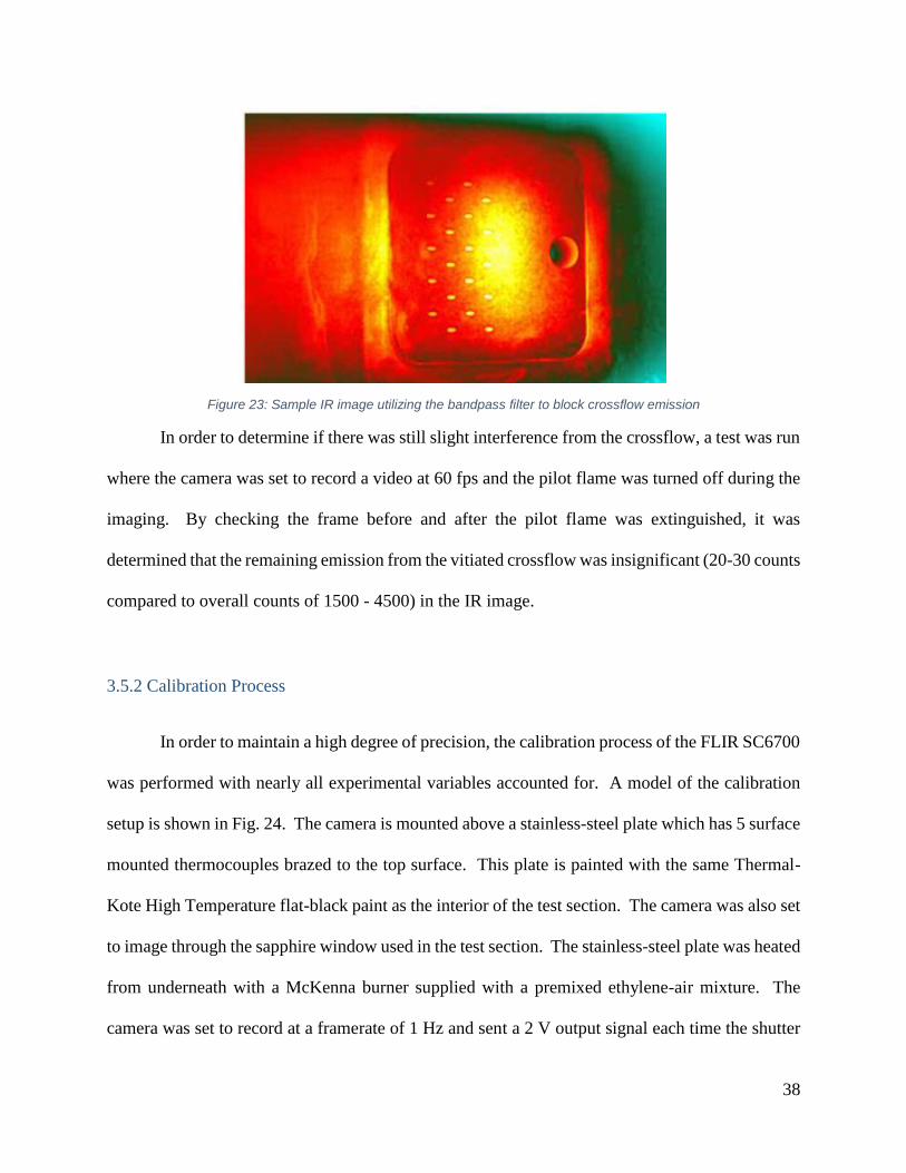
3.5.2 Calibration Process

In order to maintain a high degree of precision, the calibration process of the FLIR SC6700

was performed with nearly all experimental variables accounted for. A model of the calibration

setup is shown in Fig. 24. The camera is mounted above a stainless-steel plate which has 5 surface

mounted thermocouples brazed to the top surface. This plate is painted with the same Thermal-

Kote High Temperature flat-black paint as the interior of the test section. The camera was also set

to image through the sapphire window used in the test section. The stainless-steel plate was heated

from underneath with a McKenna burner supplied with a premixed ethylene-air mixture. The

camera was set to record at a framerate of 1 Hz and sent a 2 V output signal each time the shutter

39

opened. This 2 V output signal triggers a LABVIEW program to record temperatures for each of

the 5 thermocouples. This calibration process lasts until the plate reaches a steady state

temperature which is roughly 12 minutes with a maximum temperature of 712 K being recorded.

The bandpass filter discussed in the previous section was also in place for the calibration.

Figure 24: Model of IR camera calibration setup

The thermocouple data and raw images from the IR camera are fed into a MATLAB

program which averages the raw image counts over the location of each thermocouple pad. These

counts are then paired with each respective thermocouple reading and curve fit. A curve fit model

of 𝑇 = 𝑎 𝐼0.25 + 𝑏 was used, as this model takes into account both background noise from the

camera and the expected dependence of temperature on radiation intensity based on Eq. (2.17).

Data from multiple trials were included in the final curve fit, all of which follow the same trend.

The results of this curve fit are shown in Fig. 25 along with error bounds. These error bounds

represent 2 standard deviations from the curve and bound a confidence interval of 95.44%. For

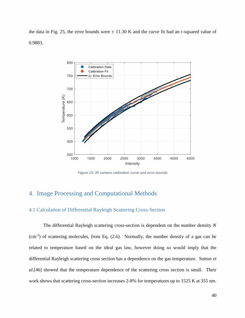
40

the data in Fig. 25, the error bounds were ± 11.30 K and the curve fit had an r-squared value of

0.9883.

Figure 25: IR camera calibration curve and error bounds

4. Image Processing and Computational Methods

4.1 Calculation of Differential Rayleigh Scattering Cross-Section

The differential Rayleigh scattering cross-section is dependent on the number density 𝑁

(cm-3) of scattering molecules, from Eq. (2.6). Normally, the number density of a gas can be

related to temperature based on the ideal gas law, however doing so would imply that the

differential Rayleigh scattering cross section has a dependence on the gas temperature. Sutton et

al.[46] showed that the temperature dependence of the scattering cross section is small. Their

work shows that scattering cross-section increases 2-8% for temperatures up to 1525 K at 355 nm.

41

This allows the use of the Loschmidt number (𝑛0 = 2.6867805 x 1019 cm-3) at STP (0℃, 1 atm) to

calculate all differential Rayleigh scattering cross-sections. Indices of refraction for each species

present in the experiment were determined using the constants and dispersion formula presented

by Gardiner et al. [47] at 355 nm:

(𝑛 − 1) ∗ 106 =𝑎

𝑏−𝜆−2 (4.1)

where n is the index of refraction at STP, a and b are constants determined by Gardiner et al. [47],

and 𝜆 is the laser wavelength in angstroms. The constants were found by using a least squares fit

program on Eq. (4.1) with values of n from other literature [47]. The accuracy of the dispersion

formula predictions and data is reported to be on the order of 10-4. Depolarization ratios for each

species were also determined for linearly polarized light. This was done by extrapolating from the

values in the work of Bogaard et al. [48] out to 355 nm. The index of refraction, depolarization

ratios for linearly polarized light, and the differential Rayleigh scattering cross-section for each

relevant species at 355 nm can be found in Table 2.

Species (n-1)*106 𝜌 * 103 𝑑𝜎

𝑑Ω * 1027 (cm2sr-1)

N2 294.52 10.960 3.0639

H2O 245.58 0.299 2.0778

CO2 437.60 42.957 7.2938

O2 265.36 28.084 2.5894

Ar 277.24 0 2.6463

OH 329.57 N/A 3.7395

CO 327.28 5.310 3.7337

H2 136.06 10.890 0.6538 Table 2: Index of refraction, depolarization ratio for linearly polarized light, and the differential Rayleigh scattering

cross-section for species relevant to the experimental flows

42

4.2 Image Processing

4.2.1 Image Filtering and Laser Profile Correction

All acquired Rayleigh scattering images were corrected for laser profile, and changes in

the laser profile throughout testing. Prior to laser profile correction, the images were processed to

identify for bad pixels (values above a specified standard deviation threshold). The standard

deviation cutoff values were chosen to be 4 for the spatial domain, and 0.5 for the intensity domain

similarly to [41]. These values were then removed and replaced utilizing an inpainting function

using average values and gradients of neighboring pixels [49]. Following this, the images were

filtered with both a bilateral and mean filter [50]. The goal of the bilateral filter was to smooth the

images while not affecting the gradients. The mean filter was used to smooth the images and

remove the camera noise sometimes referred to as “salt and pepper” noise.

Laser profile correction was performed on an image by image basis prior to this filtering

process. By utilizing image sets taken directly before the experiment (IC images), and directly

after (ENDIC images), it is possible to track the change in laser profile over the course of an

experiment. Both sets were averaged over their acquisition time 𝑡𝐼𝐶 and 𝑡𝐸𝑁𝐷𝐶𝐼𝐶, and normalized

based on the maximum intensity of the time average image 𝐼𝐼𝐶(𝑥, 𝑦, 𝑡𝐼𝐶 )̅̅ ̅̅ ̅̅ ̅̅ ̅̅ ̅̅ ̅̅ ̅̅ and 𝐼𝐸𝑁𝐷𝐼𝐶(𝑥, 𝑦, 𝑡𝐸𝑁𝐷𝐼𝐶 )̅̅ ̅̅ ̅̅ ̅̅ ̅̅ ̅̅ ̅̅ ̅̅ ̅̅ ̅̅ ̅̅ ̅̅ ̅,

creating the normalized laser profiles 𝐼𝐼𝐶,𝑛𝑜𝑟𝑚 and 𝐼𝐸𝑁𝐷𝐼𝐶,𝑛𝑜𝑟𝑚. Figure 26 shows filtered,

normalized IC and ENDIC laser profiles. The process is described mathematically in Eqs. (4.2) -

(4.3).

𝐼𝐼𝐶,𝑛𝑜𝑟𝑚 =𝐼𝐼𝐶(𝑥,𝑦,𝑡𝐼𝐶 )̅̅ ̅̅ ̅̅ ̅̅ ̅̅ ̅̅ ̅̅ ̅̅

max (𝐼𝐼𝐶(𝑥,𝑦,𝑡𝐼𝐶 )̅̅ ̅̅ ̅̅ ̅̅ ̅̅ ̅̅ ̅̅ ̅̅ ) (4.2)

𝐼𝐸𝑁𝐷𝐼𝐶,𝑛𝑜𝑟𝑚 =𝐼𝐸𝑁𝐷𝐼𝐶(𝑥,𝑦,𝑡𝐼𝐶 )̅̅ ̅̅ ̅̅ ̅̅ ̅̅ ̅̅ ̅̅ ̅̅ ̅̅ ̅̅ ̅̅

max (𝐼𝐸𝑁𝐷𝐼𝐶(𝑥,𝑦,𝑡𝐼𝐶 )̅̅ ̅̅ ̅̅ ̅̅ ̅̅ ̅̅ ̅̅ ̅̅ ̅̅ ̅̅ ̅̅ ) (4.3)

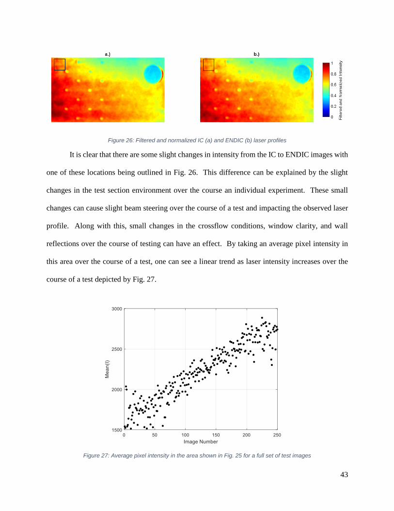
43

Figure 26: Filtered and normalized IC (a) and ENDIC (b) laser profiles

It is clear that there are some slight changes in intensity from the IC to ENDIC images with

one of these locations being outlined in Fig. 26. This difference can be explained by the slight

changes in the test section environment over the course an individual experiment. These small

changes can cause slight beam steering over the course of a test and impacting the observed laser

profile. Along with this, small changes in the crossflow conditions, window clarity, and wall

reflections over the course of testing can have an effect. By taking an average pixel intensity in

this area over the course of a test, one can see a linear trend as laser intensity increases over the

course of a test depicted by Fig. 27.

Figure 27: Average pixel intensity in the area shown in Fig. 25 for a full set of test images

44

This linear shift is utilized to determine a correction factor for each individual image 𝐾𝑖

with the index 𝑖 indicating the image number.

𝐾𝑖 =𝑖−1

249(𝐼𝐸𝑁𝐷𝐼𝐶,𝑛𝑜𝑟𝑚 − 𝐼𝐼𝐶,𝑛𝑜𝑟𝑚) + 𝐼𝐼𝐶,𝑛𝑜𝑟𝑚 (4.4)

The individual images were divided by their respective correction factor. Fig. 28 depicts a raw

LRS image and a filtered/laser corrected image.

Figure 28: Raw LRS image (a) and a filtered/corrected image (b)

4.2.2 Calculation of Temperature from LRS Images

In order to calculate temperature from the Rayleigh signal using Eq. (2.15), the calibration

constant, 𝐶 must be determined for each image. Historically, 𝐶 has been determined by performing

reference experiments with the gas composition and temperature known. From the calibration

data, 𝐶 can be directly calculated as was done by Barat et al.[28]. It is also possible to cancel out

the calibration constant by normalizing to the reference signal as was done by Sutton et al. [23].

These methods are effective for determining 𝐶, however they face a problem when the test

environment changes throughout testing. In order for these methods to hold, the experimental

setup has to be exactly the same as the reference experiment. This can be difficult for situations

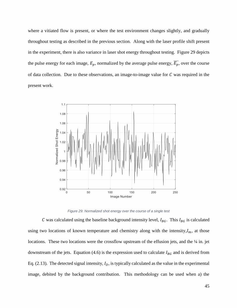
45

where a vitiated flow is present, or where the test environment changes slightly, and gradually

throughout testing as described in the previous section. Along with the laser profile shift present

in the experiment, there is also variance in laser shot energy throughout testing. Figure 29 depicts

the pulse energy for each image, 𝐸𝑝, normalized by the average pulse energy, 𝐸𝑝̅̅ ̅, over the course

of data collection. Due to these observations, an image-to-image value for 𝐶 was required in the

present work.

Figure 29: Normalized shot energy over the course of a single test

𝐶 was calculated using the baseline background intensity level, 𝐼𝐵𝐺 . This 𝐼𝐵𝐺 is calculated

using two locations of known temperature and chemistry along with the intensity,𝐼𝑚, at those

locations. These two locations were the crossflow upstream of the effusion jets, and the ¼ in. jet

downstream of the jets. Equation (4.6) is the expression used to calculate 𝐼𝐵𝐺 and is derived from

Eq. (2.13). The detected signal intensity, 𝐼𝐷, is typically calculated as the value in the experimental

image, debited by the background contribution. This methodology can be used when a) the

46

background is constant or can be ignored, and b) the background image can be taken in close

temporal proximity to the experimental images. In the case of confined flow experiments, a typical

background subtraction is not practical. Our research group has developed a technique which

utilizes “thermal pegging” at two locations in the flow to calculate the background contributions

and set a noise level for each image.

𝐼𝐷,𝑗 = 𝐼𝑚,𝑗 − 𝐼𝐵𝐺 =𝐶

𝑇𝑗∑ 𝑋𝑖

𝑘𝑖 (

𝑑𝜎

𝑑Ω)

𝑖 𝑓𝑜𝑟 𝑖 = 1,2,3 … 𝐾 𝑎𝑡 𝑙𝑜𝑐𝑎𝑡𝑖𝑜𝑛 𝑗 (4.5)

𝐼𝐵𝐺 =

𝐼𝑚,1−𝐼𝑚,2(𝑇1

(𝑑𝜎𝑑Ω

)𝑒𝑓𝑓,1

)((

𝑑𝜎𝑑Ω

)𝑒𝑓𝑓,2

𝑇2)

1−(𝑇1

(𝑑𝜎𝑑Ω

)𝑒𝑓𝑓,1

)((

𝑑𝜎𝑑Ω

)𝑒𝑓𝑓,2

𝑇2)

(4.6)

𝐶 = (𝐼𝑚,1 − 𝐼𝐵𝐺)𝑇1

(𝑑𝜎

𝑑Ω)

𝑒𝑓𝑓,1

(4.7)

where 𝑗 = 1,2 are the two locations where chemistry, temperature, and measured intensity are

known, as shown in Fig. 30. This background intensity constant for each image acts as an offset

and experimental constant as a scaling factor. A scattering signal to temperature calibration curve

is generated for each image using the calculated constant, and an empirical temperature vs

Rayleigh scattering cross-section curve. This scattering signal to temperature curve is described

by:

𝐼𝐷(𝑇) =𝐶

𝑇(

𝑑𝜎

𝑑Ω(𝑇))

𝑒𝑓𝑓+ 𝐼𝐵𝐺 (4.8)

For the flow and geometry investigated, this yields a single solution of temperature for

each intensity value. Sample curves for relative Rayleigh scattering cross-section vs temperature

and temperature vs relative detected intensity are shown in Fig. 31 for both air and CO2 jets.

47

Figure 30: Locations of known temperature, chemistry, and intensity used for calculating background intensity

Figure 31: Relative Rayleigh scattering cross-section vs temperature and temperature vs relative detected intensity

As a summary, a block diagram for image processing is shown in Fig. 31 which outlines

the entire process and has sample images at each stage of processing. This highlights the major

components of data reduction processes performed in the transformation of raw Rayleigh

scattering intensity images to temperature maps.

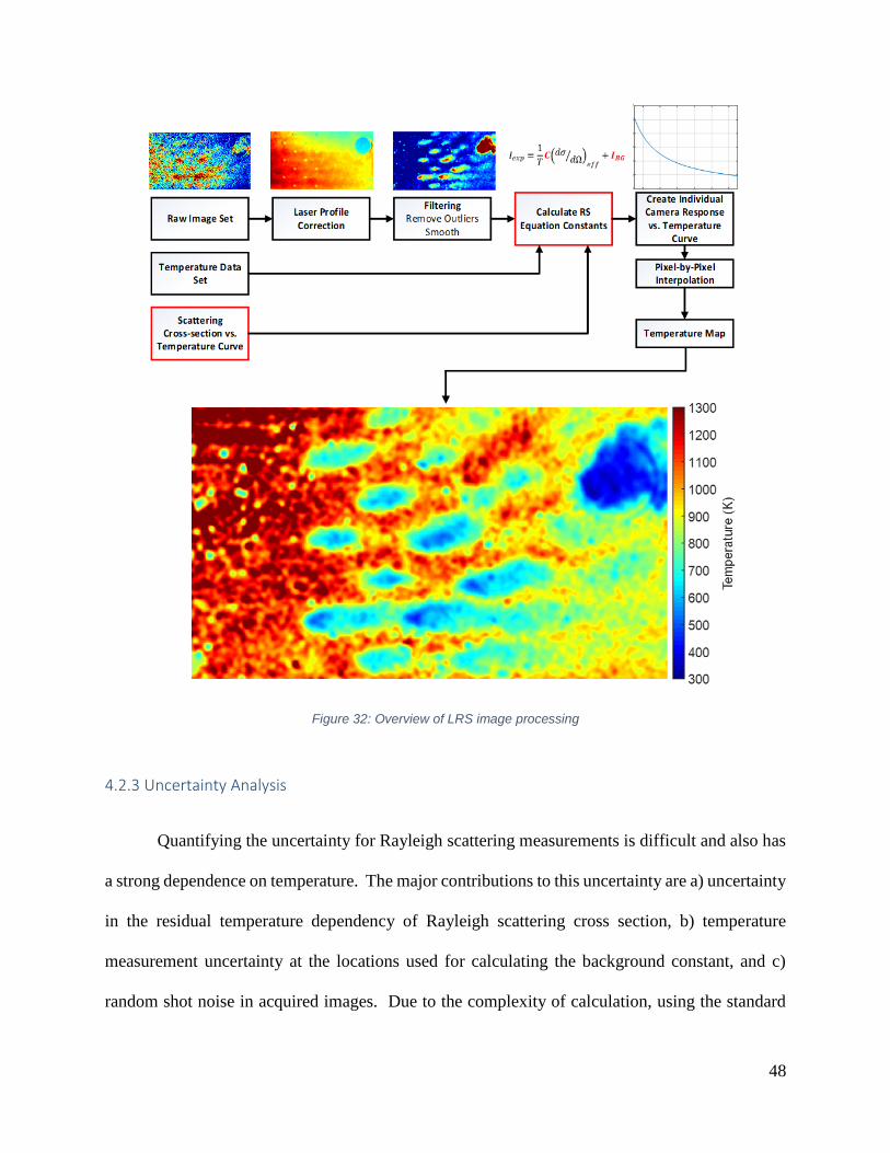
48

Figure 32: Overview of LRS image processing

4.2.3 Uncertainty Analysis

Quantifying the uncertainty for Rayleigh scattering measurements is difficult and also has

a strong dependence on temperature. The major contributions to this uncertainty are a) uncertainty

in the residual temperature dependency of Rayleigh scattering cross section, b) temperature

measurement uncertainty at the locations used for calculating the background constant, and c)

random shot noise in acquired images. Due to the complexity of calculation, using the standard

49

propagation of error variance formula is impractical. Instead, uncertainty estimates for the 3 major

contributions, (a) - (c), were fed into the model used for overall temperature calculations to

determine uncertainty limits as a function of temperature and composition of the injected jets.

Uncertainties for (a) – (c) are shown for air injection in Fig, 33. The effect caused by ignoring the

temperature dependence of the Rayleigh scattering cross-section was evaluated by utilizing

Rayleigh scattering cross-section measurements versus temperature acquired by Sutton et al. [46].

Due to the temperature pegging method and changes in mixture with temperature, overall

temperature under-prediction is below 2%. The largest contributor is shot noise and can result in

uncertainty bounds of 2-3%. By totaling the uncertainty contributions one can look at the total

uncertainty percentage as a function of temperature and jet mixture as shown in Fig. 34. The air

jets have higher levels of over prediction as expected, due to the lower overall signal levels

resulting from lower Rayleigh scattering cross-sections. For both mixtures, the overall uncertainty

levels are expected to be bounded by +3.5%, -2.5% of the calculated temperatures. Both the image

processing and uncertainty analysis are discussed in [42].

Figure 33: Sample of individual contributions to temperature calculation uncertainty for air injection

50

Figure 34: Overall temperature uncertainty (%) as a function of temperature for both air and CO2 injection

5. Results

The results presented here contain all of the data collection performed during the course of

this work, with the main results being those from the laser Rayleigh scattering studies. These data

represent the preliminary findings for this effusion cooling study and will be expanded upon in

future work. The technique for IR imaging in a hostile environment was developed and proven

for implementation in the current experiment, however results for this diagnostic could not be

collected as a result of laboratory shut down due to the unforeseen global COVID-19 pandemic.

Nevertheless, the IR imaging techniques developed will be used to collect data in the future, as

this work will be continued by another student.

51

5.1 Rayleigh Thermometry

The main goal for capturing gaseous temperature images is to validate computational

models as well as their utilization in conjunction with surface temperatures for the purpose of

determining heat transfer coefficients. However, the gas temperature fields alone provide valuable

insight into mixing and fluid mechanics of effusion cooling. To the best of our knowledge, there

is currently no publicly available literature on instantaneous, planar images of gas temperature

distribution for an effusion cooling configuration at thermal conditions relevant to GT combustors.

Initially, imaging was to be performed with the laser sheet perpendicular to the effusion

plate, taking images along the centerline of a row of holes as depicted in Fig. 35. However, it was

found that the effusion jets were only seen in approximately 1 out of every 10 images (not a set

frequency), leading to the thought that there is a significant wavering motion of the jets in and out

of the laser plane. This wavering was not always synchronous. Imaging was then performed with

the laser sheet parallel to the effusion plate with an offset from the wall in order to capture this

wavering motion. These results are presented in this section, and the test matrix is given in Table

3. The test matrix consists of a total of 21 tests, 9 with air and 12 with CO2. Data were collected

at 3.5 mm from the wall for CO2 but not air due to the different penetration depths and signal

quality for the two gas mixtures.

Figure 35: Sample filtered LRS image taken along the centerline of a single row of holes

52

Coolant Air CO2

Injection Temperature (K) 500 500

Density Ratio (Jet to Crossflow) 3.05 4.65

Blowing Ratios 5, 7, 10 5, 7, 10

Distances from Effusion Plate (mm) 2, 2.5, 3 2, 2.5, 3, 3.5

Jet Reynolds Numbers 205, 287, 410 224, 314, 449 Table 3: LRS test matrix

The blowing ratios, 𝐵𝑅 =𝜌𝑗𝑢𝑗

𝜌𝑐𝑓𝑢𝑐𝑓 , of 5, 7, and 10 were calculated using the mass average

properties and were chosen for 2 different reasons. From the existing literature, it is clear that the

most relevant blowing ratios for gas-turbine combustors are in the range of 0-10 with the majority

of studies focusing on the lower end of this range (0-3). The preliminary data presented here

focuses on the higher end of the range due to the penetration depths of the effusion jets. As

mentioned in previous sections, acquiring laser Rayleigh scattering images in close proximity to a

wall can create laser light scattering issues. With the current setup, the closest distance to the wall

where reasonably good data were able to be attained was 2 mm. At this distance, the effusion jets

were not consistently seen in the LRS images for blowing ratios less than 5. The effusion jet

injection temperature was set 500 K. Due to the low flow rate/long residence time through the

stainless-steel effusion plenum, effusion gas heats up significantly as the rig reaches a steady state.

The coolant passing through the plenum reaches a steady state temperature of 500 K rapidly when

injected. This temperature is measured just prior to the injection by a K-type thermocouple as

discussed in Section 3.1. In the future, it would be of value to both preheat and cool the effusion

mixture in order to vary the density ratio. It should also be noted that the downstream jet used for

anchoring the temperature calculation has a different injection temperature than the coolant. Since

this fluid does not have a long residence time within the ¼ in. tube, it does not reach the same

temperature. Again, this temperature is measured with a K-type thermocouple directly before

injection as described in section 3.1 and reaches a steady state temperature around 330 K. It can

53

be assumed that this jet does not significantly increase in temperature due to the proximity to the

wall and measurement location. The effusion cooling gasses of air and CO2 were chosen in order

to vary the density ratio while having similar properties (thermal conductivity, thermal diffusivity,

and viscosity).

Shown in Fig. 36 are the average images (250 frames) for the 3 blowing ratios at a distance

of 2 mm from the wall with CO2 coolant. The white circles in the images indicate the location of

each jet injection. It can be seen that as the blowing ratio decreases, the gaseous temperature at

this height increases because the average penetration depth of the jets decreases. In these images,

it would appear that there is a film covering the majority of the plate downstream of the initial

holes as more clearly seen for BR = 10 and 7. However, this is an artifact of the image averaging.

By looking at the instantaneous images, it is clear that the jets do not interact with the crossflow

in a steady manner, but instead fluctuate in all directions. Sample instantaneous images for these

same cases are shown in Fig. 37. Some of the instantaneous images do show that at times, there

is a full film coverage, however a majority of the time, the jets are maintaining an individual

trajectory and wavering side to side (as seen in looping through animations containing many

instantaneous temperature images), as well as up and down (in and out of the laser sheet). The

wavering up and down appears to be more synchronous than the side to side wavering, but is not

always synchronized between the jets. Even for the highest blowing ratio tested (10), there are

instantaneous images where no jets are observed in the image. In this section instantaneous images

may be referred to as “footprint” images due to the resemblance of footprints when all of the jets

maintain separation from one another. These footprint images revealed why there was difficulty

in obtaining centerline images and confirm that the jets were wavering as suspected.

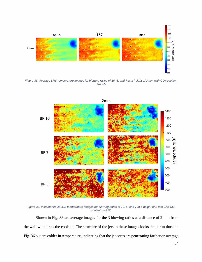
54

Figure 36: Average LRS temperature images for blowing ratios of 10, 5, and 7 at a height of 2 mm with CO2 coolant, s=4.65

Figure 37: Instantaneous LRS temperature images for blowing ratios of 10, 5, and 7 at a height of 2 mm with CO2 coolant, s=4.65

Shown in Fig. 38 are average images for the 3 blowing ratios at a distance of 2 mm from

the wall with air as the coolant. The structure of the jets in these images looks similar to those in

Fig. 36 but are colder in temperature, indicating that the jet cores are penetrating farther on average

55

into the crossflow than the CO2 jets for the same blowing ratio. This can also be seen in the

instantaneous images shown in Fig. 39. The colder temperature indicates longer penetration depth

because the jets are the same temperature when injected, therefore to achieve this colder

temperature at the same height on an average basis, the jets must be penetrating further on average.

As mentioned in Section 4.2, the acquired laser Rayleigh scattering signal from air injection is

about half of that from CO2 injection due to their effective Rayleigh scattering cross-sections. This

causes the instantaneous LRS images for air to have a higher degree of noise present. This noise

is not completely filtered out in order to preserve the original image and maintain the same filter

properties for all images.

Figure 38: Average LRS temperature images for blowing ratios of 10, 5, and 7 at a height of 2 mm with air coolant,

s=3.05

56

Figure 39: Instantaneous LRS temperature images for blowing ratios of 10, 5, and 7 at a height of 2 mm with air coolant, s=3.05

For a better direct comparison between the two coolants, average LRS images for both at

heights of 2, 2.5, and 3 mm and a blowing ratio of 5 can be seen in Fig. 40. From this, it is apparent

that the penetration depth of air is greater than that of CO2. This is likely due to the blowing ratio

flow parameter. Since the density of the air injected is lower than that of the CO2, in order to

maintain the same blowing ratio, velocity must be increased. For a blowing ratio of 5, the initial

velocity of the CO2 jets was 8.05 m/s and the initial velocity of the air jets was 12.23 m/s. While

blowing ratio is widely used as a scaling parameter for heat transfer and cooling effectiveness

analysis, this shows that it may not be the ideal scaling parameter for the fluid mechanics of the

problem. Prior work from the lab [39], [41], [42] has shown the jet to crossflow momentum ratio,

57

𝐽 =𝜌𝑗𝑢𝑗

2

𝜌𝑐𝑓𝑢𝑐𝑓2 (5.1)

is the primary scaling parameter for jet trajectories and mixing in an orthogonal injection

configuration such as jets injected into a crossflow. While these jets are angled in the flow

direction, the same scaling may apply and further tests should be conducted by matching 𝐽 between

the two coolants. Table 4 includes the blowing ratio, gas density, initial velocity, and 𝐽 for all flow

conditions based on a crossflow density of 0.2309 kg/m3 and velocity of 7.6 m/s. Sample footprint

images for the cases in Fig. 40 can also be seen in Fig. 41.

Figure 40:Average LRS temperature images for air and CO2 at 3 different heights and a blowing ratio of 5

Coolant BR 𝝆 (kg/m3) Initial Velocity

(m/s)

Momentum

Ratio

Jet Reynolds

Number

CO2

5

1.075

8.05 5.37 224

7 11.27 10.52 314

10 16.10 21.46 449

Air

5

0.708

12.23 8.16 205

7 17.12 15.98 287

10 24.47 32.62 410 Table 4: Test matrix flow conditions

58

Figure 41: Instantaneous LRS temperature images for air and CO2 at 3 different heights and a blowing ratio of 5

Figure 42 shows an average and 2 instantaneous LRS temperature image for CO2 injection

at a distance of 3 mm and blowing ratio of 5. Looking at the average image, it appears there are

no jets present, however the instantaneous images show that at times, there is full jet core

59

penetration into the laser plane. The wavering motion of these jets is quite significant and can

impact the effectiveness of the film. If the film is constantly separating from the wall, or not

maintaining full coverage, then the liner could be exposed to high gas temperatures intermittently.

In order to quantify this motion, the root mean square deviation (%) of each image set was

calculated (250 frames per set).

𝑅𝑀𝑆 𝐷𝑒𝑣𝑖𝑎𝑡𝑖𝑜𝑛𝑖,𝑗 (%) =100

𝑇𝑚𝑒𝑎𝑛 𝑖,𝑗∗ √∑ (𝑇𝑚𝑒𝑎𝑛 𝑖,𝑗−𝑇𝑖,𝑗)

2 𝑛

𝑘=1

𝑛 (5.2)

where n is the total number of images, and the subscripts i and j indicate the pixel location. This

processing highlights locations in the images where there is significant motion/wavering. Shown

in Fig. 43 are these RMS deviation (%) images for CO2 injection at heights of 2, 2.5, and 3 mm for

a blowing ratio of 7. From these, one can see that as the distance from the wall is increased, the

frequency and magnitude of these fluctuations decreases while the effusion jets mix with the

crossflow. The location where a majority of the fluctuations occur is the locations between each

the of the jets. This is expected as that is where a majority of the effusion jet interaction will occur.

The individual jets wavering back and forth will interact with one another, enhancing turbulence,

which affects mixing between the effusion jets and the main flow. This interaction of jets can be

observed in Fig. 44 which is an instantaneous LRS temperature image of CO2 injection for a

blowing ratio of 10 at a distance of 3 mm. The wavering up and down (in and out of the laser

plane) is also most likely caused by jet interaction, with an upstream jet impacting downstream

jets causing large scale rollups/vortices on the windward side. The jet to crossflow interaction

may also contribute to these rollups by entrainment as seen in [42].

60

Figure 42: Average and instantaneous LRS temperature images for CO2 injection at 3 mm and blowing ratio of 5

Figure 43: RMS deviation from the mean image for CO2 injection at a blowing ratio of 7

Figure 44: Instantaneous LRS temperature image of CO2 injection at a blowing ratio of 10 and distance of 3mm from the wall highlighting the individual jet interactions

61

Shown in Fig. 45 are RMS deviation (%) images for air injection at heights of 2, 2.5, and

3 mm for a blowing ratio of 7. Comparing this to Fig. 43, it is clear that the air jets experience

significantly more motion, at the same experimental conditions, than the CO2 jets with the largest

fluctuations occurring in the same regions. This difference in motion could be due to a multitude

of factors. As mentioned earlier, prior work from our laboratory [42] has found that the fluid

dynamics for orthogonal jet injection is heavily dependent on the jet to crossflow momentum ratio.

Therefore, this difference in jet motion could be attributed to variance in 𝐽. However, since the

scaling parameter used here is blowing ratio, it can be stated that at a set blowing ratio, as density

ratio decreases, motion of the effusion jets increases. Fig. 45 also follows the same trend as Fig.

43 with the fluctuations decreasing as distance from the wall increases.

Figure 45: RMS deviation from the mean image for air injection at a blowing ratio of 7

While the flow interaction may the source of these fluctuations, it is important to look at

all possibilities for the observed trends. In this case, one variable possibility could be the quality

of holes drilled on the effusion plate. The effusion plate was laser drilled, which is the often-used

manufacturing method for effusion cooling holes due to its relative low cost and shorter

manufacturing time. However, this process can leave slag and jagged edges on the interior and

62

around the hole exit. These unconformities could trip the flow and cause vortex shedding and

turbulence in the effusion jets prior to injection into the crossflow. The turbulence seen in the

images is not inherent to flow due to the low Reynolds numbers and therefore must be caused by

jet interaction with either the crossflow, other jets, or the hole geometry. In order to better

understand the hole geometry, microscopic images were taken of the holes and two of these images

are shown in Fig. 46. These two holes are located directly next to each other on the plate but one

can see that they are quite different. Hole (a) has an elliptical exit but has jagged edges and a large

piece of slag near the exit. Hole (b) has a different shape of the hole exit than (a) and is non-

symmetrical while also having visibly jagged edges. This lack of consistency from hole to hole

could be another reason why each jet appears to interact with the flows differently on an

instantaneous basis.

Figure 46: Microscopic images to two laser drilled holes on the test plate

In order to separate the two problems, and better understand the effect of hole geometry on

the flow interactions, future work should be conducted to study the effect of hole manufacturing

method on the effusion jets. If a manufacturing method can yield a smoother interior and exit of

the hole, then this may better allow full film coverage to be maintained as the amount of local

turbulence could be decreased. Differing manufacturing methods should be investigated; this

would allow for a wide comparison between both the geometry and the flow interactions while

63

holding flow conditions constant. For now, it is believed that these imperfections do have an

impact on the flow but the extent of that is unknown and must be quantified in the future with

further testing.

Lastly, a repeatability test was performed in which the same test cases (CO2 injection,

imaging 2.5 mm from the wall) were run 9 days after the original tests to ensure that the

experimental results were repeatable. The average LRS temperature images are shown in Fig. 47

and the separate tests have less than 10% difference between each other on a pixel by pixel basis.

These slight differences could be caused by small changes in the crossflow temperature on a given

day. As discussed in section 3.2, there is slight crossflow temperature variation day to day, due to

both lab and atmospheric conditions, but all the data are recorded for each test case.

Figure 47: Repeatability test cases for CO2 injection at a distance of 2.5 mm from the wall

All average and sample instantaneous LRS temperature fields can be found in Appendix A.

64

6. Conclusion and Future Work

Over the past 60 years, research has been conducted to study and investigate the heat

transfer characteristics of the effusion jet cooling of combustor liners. This research, which

initially began with simple time averaged thermocouple measurements of surface temperature, has

blossomed into a vast array of complex diagnostics and studies which has led to the development

of current gas-turbine combustor cooling. As data acquisition and analysis techniques have

improved, understanding of the heat transfer phenomena has matured and been widely adopted

throughout the scientific community. However, current simulation and modeling software can still

not accurately predict heat transfer in combustor relevant environments without good quality

experimental data to test and anchor those simulation results. With the hot and hostile operating

conditions of a combustor being difficult to replicate in a laboratory setting, there is currently a

lack of experimental data at relevant temperatures and geometries as discussed in the introduction.

The current combustor liner design process is based on past research on low temperature

heat transfer experimental results and empirical correlations from those studies incorporated into

some standard work. The current state of the art for combustor liner cooling predictions are not at

a level to support the development of the modern high-intensity combustor cooling schemes. In

order to improve this process, an experimental methodology for studying the fundamentals of

effusion cooling in a hot (1500 K), vitiated crossflow was developed. This methodology allows

for instantaneous imaging of gas phase temperature near the surface where the jets are injected.

To the best of the author’s knowledge, there is currently no publicly available literature that reports

measurements of gas temperature fields in the effusion cooling film.

65

In this study, a planar laser Rayleigh scattering temperature imaging technique was used

to measure gas temperature distributions to gain insight into heat transfer and fluid dynamics of

this problem. Along with the gas phase temperature imaging, an experimental methodology was

developed for IR imaging of the effusion plate to obtain surface temperature. This methodology

is unique in that it has to account for radiative emission from a variety of sources including the

vitiated flow, the viewing window, and other environmental concerns. Unfortunately, data were

not acquired for IR imaging due to an unforeseen circumstance discussed in Section 5. However,

the methodology was developed and data will be acquired in the future, as this work will be

continued by another student.

Preliminary LRS studies were performed for blowing ratios of 5, 7, and 10 for both air

(s=3.05) and CO2 (s=4.65) injection; 𝐵𝑅 =𝜌𝑗𝑢𝑗

𝜌𝑐𝑓𝑢𝑐𝑓 , 𝑠 =

𝜌𝑗

𝜌𝑐𝑓. These images were taken parallel

to the injection plane at heights of 2, 2.5, 3, and 3.5 mm. The injection gas temperature was held

constant at 500K and the nominal crossflow conditions were 7.6 m/s and bulk temperature of 1500

K. Initial imaging highlighted the wavering motion of the jets which can be attributed to 3 different

sources: 1.) Flow interactions between the individual jets, 2.) Entrainment of crossflow, and 3.)

Geometry of the effusion jet hole creating turbulence prior to injection.

It was found that when blowing ratio was held constant, and the jet to crossflow density

ratio (𝑠) was decreased, overall fluctuations in the flow increased. Along with this, at a set blowing

ratio, penetration depth of the jets decreases with increasing density ratio. This could be attributed

to differences in the jet to crossflow momentum ratio (𝐽). As found in previous work [41], [42],

jet trajectory for orthogonal jet injection is strongly dependent on 𝐽. Further studies should be

66

performed that match 𝐽 between the two mixtures rather than blowing ratio in order to investigate

its effect on penetration depth for non-orthogonal jets.

The most important takeaway is that the average LRS temperature images are not a valid

representation of what is happening on an instantaneous basis. The instantaneous images reveal

that while there may appear to full film coverage on average, this is almost never the case at any

given point in time. This implies that steady RANS simulations cannot accurately predict the fluid

mechanics of this problem due to significant flow instabilities observed in the experiments. If

combustor design is based on average flow and thermal fields, the instantaneous motion could lead

to large deviations from these averages in the film and possibly lead to combustor liner failure.

Further understanding of this film development is important to its initiation at the upstream

end of a combustor liner. Different geometries should be investigated in the future which feature

a variety of hole patterns. Some recommendations for future designs include:

1.) A larger array of cooling holes to better view the transition from film initiation to full

film coverage.

2.) Densely packed effusion jets to understand the effect of jet to jet spacing on film

development.

3.) Varying the manufacturing method for a single plate design to quantify the effect that

hole geometry may have on the flow.

Along with these recommendations for design, some recommendations for future work include:

1.) Implementing the developed IR imaging methodology on both the front and back side

of the effusion plate in order to determine heat flux through the plate.

67

2.) Performing center plane imaging such as in Fig. 35 in order to view the interaction

between the crossflow and effusion jets.

3.) Investigations spanning all equivalence ratio ranges and fuels encountered in

combustion devices to assess the influences of the cooling flows on the chemistry of

the combustion flow field.

68

References [1] N. P. Padture, “Advanced structural ceramics in aerospace propulsion,” Nat. Mater., vol.

15, no. 8, pp. 804–809, Aug. 2016, doi: 10.1038/nmat4687.

[2] D. E. Metzger, H. J. Carper, and L. R. Swank, “Heat Transfer With Film Cooling Near

Nontangential Injection Slots,” J. Eng. Power, vol. 90, no. 2, pp. 157–162, Apr. 1968, doi:

10.1115/1.3609155.

[3] P. Renze, W. Schröder, and M. Meinke, “Large-eddy simulation of interacting film cooling

jets,” ASME GT, no. 59164, 2009.

[4] G. Cerri, A. Giovannelli, L. Battisti, and R. Fedrizzi, “Advances in effusive cooling

techniques of gas turbines,” Appl. Therm. Eng., vol. 27, no. 4, pp. 692–698, Mar. 2007, doi:

10.1016/j.applthermaleng.2006.10.012.

[5] A. B. Wassell and J. K. Bhangu, “The Development and Application of Improved

Combustor Wall Cooling Techniques,” in Volume 1A: General, New Orleans, Louisiana,

USA, Mar. 1980, p. V01AT01A066, doi: 10.1115/80-GT-66.

[6] K. M. B. Gustafsson and T. G. Johansson, “An Experimental Study of Surface Temperature

Distribution on Effusion-Cooled Plates,” J. Eng. Gas Turbines Power, vol. 123, no. 2, pp.

308–316, Apr. 2001, doi: 10.1115/1.1364496.

[7] H. H. Cho and R. J. Goldstein, “Heat (Mass) Transfer and Film Cooling Effectiveness With

Injection Through Discrete Holes: Part II—On the Exposed Surface,” J. Turbomach., vol.

117, no. 3, pp. 451–460, Jul. 1995, doi: 10.1115/1.2835681.

[8] A. C. Shrager, K. A. Thole, and D. Mongillo, “Effects of Effusion Cooling Pattern Near the

Dilution Hole for a Double-Walled Combustor Liner—Part 1: Overall Effectiveness

Measurements,” J. Eng. Gas Turbines Power, vol. 141, no. 1, p. 011022, Aug. 2018, doi:

10.1115/1.4041148.

[9] R. E. Mayle and F. J. Camarata, “Multihole Cooling Film Effectiveness and Heat Transfer,”

J. Heat Transf., vol. 97, no. 4, pp. 534–538, Nov. 1975, doi: 10.1115/1.3450424.

[10] J. J. Scrittore, K. A. Thole, and S. W. Burd, “Investigation of Velocity Profiles for Effusion

Cooling of a Combustor Liner,” J. Turbomach., vol. 129, no. 3, pp. 518–526, Jul. 2007, doi:

10.1115/1.2720492.

[11] B. Facchini, L. Tarchi, L. Toni, and A. Ceccherini, “Adiabatic and Overall Effectiveness

Measurements of an Effusion Cooling Array for Turbine Endwall Application,” J.

Turbomach., vol. 132, no. 4, p. 041008, Oct. 2010, doi: 10.1115/1.3213555.

[12] A. Andreini et al., “Density Ratio Effects on the Cooling Performances of a Combustor

Liner Cooled by a Combined Slot/Effusion System,” in Volume 4: Heat Transfer, Parts A

and B, Copenhagen, Denmark, Jun. 2012, pp. 903–914, doi: 10.1115/GT2012-68263.

[13] S. Papell, “Effect On Faseous Film Cooling Of Coolant Injection Through Angled Slots

And Normal Holes,” U. S. Natl. Aeronaut. Space Adm. NASA Tech. Note Wash. Natl.

Aeronaut. Space Adm., Sep. 1960.

[14] H. Choe, W. Kays, and R. Moffat, “Turbulent boundary layer on a full-coverage film-

cooled surface: An experimental heat transfer study with normal injection,” U. S. Natl.

Aeronaut. Space Adm. NASA Tech. Note Wash. Natl. Aeronaut. Space Adm., Jan. 1976.

[15] K. Miller and M. Crawford, “Numerical Simulation of Single, Double, and Multiple Row

Film Cooling Effectiveness and Heat Transfer,” ASME 1984 Int. Gas Turbine Conf. Exhib.,

Jun. 1984, doi: 10.1115/84-GT-112.

69

[16] Y. Liu, P. Jiang, and Y. Wang, “Flow and heat transfer characteristics of two effused

cooling models: transpiration cooling and full coverage film cooling,” Proc. 2nd ISJPPE,

vol. 2, pp. 615–622, 2008.

[17] D. Bohn and N. Moritz, “Numerical study on inner hole shaping of full coverage cooled

multi-layer plates,” Front. Energy Power Eng. China, vol. 3, Jun. 2009, doi:

https://doi.org/10.1007/s11708-009-0041-x.

[18] A. Andreini, A. Ceccherini, B. Facchini, L. Tarchi, and L. Toni, “Hole spacing effect on

adiabatic effectiveness of effusion cooling arrays for turbine endwall application,” Proc.

8th Eur. Turbomach. Conf., pp. 553–567, 2009.

[19] Y. Hu and H. Ji, “Numerical study of the effect of blowing angles on cooling effectiveness

of an effusion cooling,” ASME GT2004, 2004.

[20] T. F. Fric, R. P. Campbell, and M. G. Rettig, “Quantitative Visualization of Full-Coverage

Discrete-Hole Film Cooling,” in Volume 3: Heat Transfer; Electric Power; Industrial and

Cogeneration, Orlando, Florida, USA, Jun. 1997, p. V003T09A064, doi: 10.1115/97-GT-

328.

[21] S. McGhee, “Thermal Imaging Camera for Effusion Cooling Research,” Queens

University, Kingston, Ontario, Canada, 1999.

[22] J. Sutton, “Mixture Fraction and Scalar Dissipation Rate Imaging in Turbulent

Nonpremixed Flames Near Extinction,” Ph.D. Dissertation, Dept. of Aerospace

Engineering, University of Michigan, Ann Arbor, MI, 2005.

[23] C. Arndt, M. Papageorge, F. Fuest, J. Sutton, W. Meier, and M. Aigner, “The role of

temperature, mixture fraction, and scalar dissipation rate on transient methane injection and

auto-ignition in a jet in hot coflow burner,” Combust. Flame, vol. 167, pp. 60–71, 2016.

[24] D. Feikema, D. Everest, and J. Driscoll, “Images of Dissipation Layers to Quantify Mixing

withing a Turbulent Jet,” AIAA, vol. 34, no. 12, Dec. 1996.

[25] R. Barlow and A. Karpetis, “Measurements of Scalar Variance, Scalar Dissipation, and

Length Scales in Turbulent Piloted Methane/Air Jet Flames,” Flow Turbul. Combust., vol.

72, no. 2–4, 2004.

[26] J. Balla and J. Everhart, “Rayleigh Scattering Density Measurements, Cluster Theory, and

Nucleation Calculations at Mach 10,” AIAA, vol. 50, no. 3, Mar. 2012.

[27] R. Gordon, M. Assaad, and E. Mastorakos, “Simultaneous Rayleigh temperature, OH- and

CH2O-LIF imaging of methane jets in a vitiated coflow,” Combust. Flame, vol. 155, pp.

181–195, 2008.

[28] R. Barat, J. Longwell, A. Sarofim, S. Smith, and E. Bar-Ziv, “Laser Rayleigh scattering for

flame thermometry in a toroidal jet stirred combustor,” Appl. Opt., vol. 30, no. 21, pp.

3003–3010, 1991.

[29] J. W. S. 3rd Baron Rayleigh, “On the Light From the Sky, its Polarization and Colour,” M

R Luo Ed Bedford MA Camb. Res. Lab. 1870, Reproduced in 1966.

[30] R. Miles, W. Lempert, and J. Forkey, “Laser Rayleigh scattering,” Meas. Sci. Technol., vol.

12, 2001.

[31] T. Buzug, Computed Tomography, From Photon Statistics to Modern Cone Beam CT.

2008.

[32] D. Long, “The Raman Effect: A Unified Treatment of the Theory of Raman Scattering by

Molecules,” West Sussex UK John Wiley Sons, 2002.

[33] T. Bergman, A. Lavine, F. Incropera, and D. Dewitt, Fundamentals of Heat and Mass

Transfer, 7th ed. John Wiley & Sons Inc.

70

[34] Ravindra, Sopori, Gocke, and Cheng, “Emissivity Measurements and Modeling of Silicon-

Related Materials: An Overview,” Int. J. Thermophys., vol. 22, no. 5, pp. 1593–1611, Sep.

2001.

[35] “Data Sheet: Commercial Grade Fused Quartz,” UQG Optics.

https://www.uqgoptics.com/wp-content/uploads/2019/03/Commercial-Grade-Fused-

Quartz.pdf.

[36] “Fused Silica,” Precision Micro Optics. http://www.pmoptics.com/Fused_Silica.html.

[37] M. Babladi, “Radiative Properties of IR Materials,” New Jersey Institute of Technology.

[38] “Atmospheric Absorption & Transmission,” Humboldt State University.

http://gsp.humboldt.edu/OLM/Courses/GSP_216_Online/lesson2-1/atmosphere.html.

[39] J. Wagner, S. Grib, M. Renfro, and B. Cetegen, “Flowfield measurements and flame

stabilization of a premixed reacting jet in vitiated crossflow,” Combust. Flame, vol. 162,

no. 10, 2015.

[40] H. Bell and R. Mehta, ““Boundary-layer predictions for small low-speed contractions.,”

AIAA J, vol. 27, no. 3, Mar. 1989, doi: 10.2514/3.10122.

[41] K. Linevitch, “Near Field Mixing Characteristics of a Variable Density Non-Reacting Jet in

a Hot Vitiated Crossflow,” Master’s Thesis, University of Connecticut, 2018.

[42] J. W. Dayton, B. K. Poettgen, K. Linevitch, and B. M. Cetegen, “Non-isothermal mixing

characteristics in the extreme near-field of a turbulent jet in hot crossflow,” Phys. Fluids,

vol. 31, no. 12, p. 125104, Dec. 2019, doi: 10.1063/1.5127283.

[43] Goodwin, Moffat, and Speth, CANTERA: An Object-Oriented SoftwareToolkit for

Chemical Kinetics, Thermodynamics, and Transport Processes. 2017.

[44] H. Wang et al., USC Mech Version II. High-Temperature Combustion Reaction Model of

H2/CO/C1-C4 Compounds. 2007.

[45] I. E. Gordon et al., “The HITRAN2016 molecular spectroscopic database,” J. Quant.

Spectrosc. Radiat. Transf., vol. 203, pp. 3–69, Dec. 2017, doi: 10.1016/j.jqsrt.2017.06.038.

[46] J. Sutton and J. Driscoll, “Rayleigh Scattering Cross Sections of Combustion Species at

266, 355, and 532 nm for Thermometry Applications,” Opt. Lett., vol. 29, no. 22, pp. 2620–

2622, 2004.

[47] W. Gardiner, Y. Hidaka, and T. Tanzawa, “Refractivity of Combustion Gases,” Combust.

Flame, vol. 40, pp. 213–219, 1981.

[48] M. Bogaard, A. Buckingham, R. Pierens, and A. White, “Rayleigh Scattering

Depolarization Ratio and Molecular Polarizability Anistropy for Gases,” J. Chem. Soc.

Faraday Trans. I, vol. 74, no. 0, pp. 3008–3015, 1978.

[49] D’Errico, inpaint_nans. MATLAB Central File Exchange, 2012.

[50] C. Tomasi and R. Manduchi, “Bilateral Filtering for Fray and Color Images,” presented at

the Sixth International Conference on Computer Vision, Bombay, 1998.

71

Appendix A: Full Data Sets

Figure 48: Average LRS temperature images for all CO2 cases, s=4.65

72

Figure 49: Sample instantaneous LRS temperature images for all CO2 cases, s=4.65

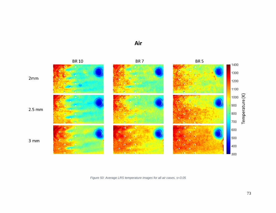
73

Figure 50: Average LRS temperature images for all air cases, s=3.05

74

Figure 51: Sample instantaneous LRS temperature images for all air cases, s=3.05

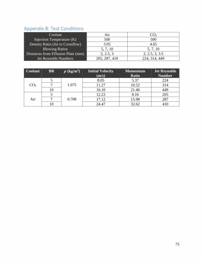
75

Appendix B: Test Conditions Coolant Air CO2

Injection Temperature (K) 500 500

Density Ratio (Jet to Crossflow) 3.05 4.65

Blowing Ratios 5, 7, 10 5, 7, 10

Distances from Effusion Plate (mm) 2, 2.5, 3 2, 2.5, 3, 3.5

Jet Reynolds Numbers 205, 287, 410 224, 314, 449

Coolant BR 𝝆 (kg/m3) Initial Velocity

(m/s)

Momentum

Ratio

Jet Reynolds

Number

CO2

5

1.075

8.05 5.37 224

7 11.27 10.52 314

10 16.10 21.46 449

Air

5

0.708

12.23 8.16 205

7 17.12 15.98 287

10 24.47 32.62 410