
Experimental Investigation of Active Wingtip Vortex ...
139
EXPERIMENTAL INVESTIGATION OF ACTIVE WINGTIP VORTEX CONTROL USING SYNTHETIC JET ACTUATORS A Thesis presented to the Faculty of California Polytechnic State University San Luis Obispo In Partial Fulfillment of the Requirements for the Degree Master of Science in Aerospace Engineering by Peter J. Sudak August 2014
Transcript of Experimental Investigation of Active Wingtip Vortex ...

EXPERIMENTAL INVESTIGATION OF ACTIVE WINGTIP VORTEX
CONTROL USING SYNTHETIC JET ACTUATORS
A Thesis
presented to
the Faculty of California Polytechnic State University
San Luis Obispo
In Partial Fulfillment
of the Requirements for the Degree
Master of Science in Aerospace Engineering
by
Peter J. Sudak
August 2014

ii
© 2014
Peter J. Sudak
ALL RIGHTS RESERVED

iii
COMMITTEE MEMBERSHIP
TITLE: Experimental Investigation of Active Wingtip Vortex
Control Using Synthetic Jet Actuators
AUTHOR: Peter J. Sudak
DATE SUBMITTED: August 2014
COMMITTEE CHAIR: Jin Tso, Ph.D.
Professor of Aerospace Engineering
COMMITTEE MEMBER: Russell Westphal, Ph.D.
Professor of Mechanical Engineering
COMMITTEE MEMBER: Rob McDonald, Ph.D.
Associate Professor of Aerospace Engineering
COMMITTEE MEMBER: Faysal Kolkailah, Ph.D.
Professor of Aerospace Engineering

iv
ABSTRACT
Experimental Investigation of Active Wingtip Vortex Control using Synthetic Jet
Actuators
Peter J. Sudak
An experiment was performed in the Cal Poly Mechanical Engineering 2x2 ft wind tunnel
to quantify the effect of spanwise synthetic jet actuation (SJA) on the drag of a NACA 0015
semispan wing. The wing, which was designed and manufactured for this experiment, has an
aspect ratio of 4.20, a span of 0.427 m (16.813”), and is built around an internal array of
piezoelectric actuators, which work in series to create a synthetic jet that emanates from the
wingtip in the spanwise direction. Direct lift and drag measurements were taken at a Reynolds
Number of 100,000 and 200,000 using a load cell/slider mechanism to quantify the effect of
actuation on the lift and drag. It was found that the piezoelectric disks used in the synthetic jet
actuators cause structural vibrations that have a significant effect on the aerodynamics of the
NACA 0015 model. The experiment was performed in a way as to isolate the effect of vibration
from the effect of the synthetic jet on the lift and drag. Lift and drag data was supported with
pressure readings from 60 pressure ports distributed in rows along the span of the wing. Oil
droplet flow visualization was also performed to understand the effect of SJA near the wingtip.
The synthetic jet and vibration had effects on the drag. The synthetic jet with vibration
decreased the drag only slightly while vibration alone could decrease drag significantly from
11.3% at α = 4° to 23.4% at α = 10° and Re = 100,000. The lift was slightly increased with a
slight increase due to the jet and showed a slight increase due to vibration. Two complete rows of
pressure ports at 2y/b = 37.5% and 85.1% showed changes in lift due to actuation as well. The
synthetic jet increased the lift near the wingtip at 2y/b = 85.1% and had little to no effect inboard
at the 37.5% location, hence, the synthetic jet changes the lift distribution on the wing. Oil flow
visualization was used to support this claim. Without actuation, the footprint of the tip vortex was
present on the upper surface of the wing. With actuation on, the footprint disappeared suggesting
the vortex was pushed off the wingtip by the jet. It is possible that the increased lift with actuation
can be caused by the vortex being pushed outboard.
Keywords: Active Flow Control, NACA 0015, Semispan Testing, Synthetic Jet, Piezoelectric
Actuators, Design, Wingtip Vortex, Hot-wire.

v
ACKNOWLEDGMENTS
First of all, I would like to thank my parents for supporting me not only while I worked on
my Thesis but throughout my college career. I could not have made it without you and I cannot
even express how grateful I am. Thank you very much. Acknowledgments
I would like to thank Dr. Tso for taking me on as his graduate student. Dr. Tso, thank you
for always being readily available to offer your support and providing the resources I needed to
complete my Thesis. It was a pleasure having you as an advisor.
I would like to give a big thank you to Dr. Westphal for letting me use the Mechanical
Engineering wind tunnel while the Aero tunnel was being repaired. Also, thank you for always
being willing to share your expert advice and letting me use all the cool equipment in the ME
tunnel.
I would like to thank Dr. McDonald for serving on my committee and answering questions
that I had. It was helpful to hear your perspective on various aspects of this project.
I would like to thank Dr. Kolkailah for accepting a position on my committee last minute
after one member became unavailable. I hope you found my work interesting.
I would like to thank Cody Thompson for letting me use his machine shop and buying me
supplies in a moment’s notice whenever needed. Your assistance helped me finish this project it a
“timely” manner
Finally yet importantly, I would like to thank Alan L’Esperance for his help in all aspects of
this project from helping me with the manufacture of the wing to showing me how to use various
pieces of test equipment that were used for this Thesis.

vi
TABLE OF CONTENTS
LIST OF TABLES ix
LIST OF FIGURES x
NOMENCLATURE xiv
1 Introduction 1
1.1 Literature Survey ............................................................................................................. 1
1.2 Purpose ............................................................................................................................ 3
1.3 Background ...................................................................................................................... 5
1.3.1 Wing Tip Vortices............................................................................................. 5
1.3.2 Lift-Induced Drag ............................................................................................. 6
1.3.3 Zero-Net Mass-Flux Actuators ......................................................................... 6
1.3.4 Momentum Coefficient ..................................................................................... 8
1.3.5 Non-Dimensional Frequency, F+ ...................................................................... 9
2 Design and Manufacture of Experiment 10
2.1 Manufacturing Equipment ............................................................................................. 10
2.1.1 Haas VF-3 ....................................................................................................... 10
2.1.2 Haas Super Minimill 2 .................................................................................... 12
2.1.3 Haas TL-1 ....................................................................................................... 12
2.1.4 Universal Laser Systems VLS6.60 Laser cutter ............................................. 13
2.2 Synthetic Jet Actuator .................................................................................................... 14
2.3 NACA 0015 Semispan Model ....................................................................................... 18
2.3.1 Model Accuracy .............................................................................................. 36
2.4 Load Cell Support Structure .......................................................................................... 37
3 Experimental Apparatus 41
3.1 LabVIEW ...................................................................................................................... 41
3.2 Wind Tunnel .................................................................................................................. 43
3.3 Pressure Measurement System ...................................................................................... 44

vii
3.3.1 ZOC33/64Px ................................................................................................... 44
3.3.2 RADBASE 3200-EXT .................................................................................... 45
3.4 Linear Amplifier ............................................................................................................ 45
3.5 Bimorph Actuator Disk ................................................................................................. 46
3.6 Load Cell ....................................................................................................................... 47
3.7 NACA 0015 Semispan Model ....................................................................................... 47
3.8 Hotwire Anemometer System........................................................................................ 49
3.8.1 Thermal Anemometer ..................................................................................... 50
3.8.2 Hotwire Sensor ............................................................................................... 50
3.8.3 Automatic Velocity Calibrator ........................................................................ 51
3.8.4 Hotwire Fixture ............................................................................................... 52
4 Analysis 54
4.1 Momentum Coefficient Calculation .............................................................................. 54
4.2 Coefficient of Pressure Calculation ............................................................................... 54
4.2.1 Tunnel Calibration .......................................................................................... 55
4.2.2 Solid & Wake Blockage.................................................................................. 55
4.2.3 Buoyancy Correction ...................................................................................... 56
4.3 Sectional Force Coefficients .......................................................................................... 58
4.4 Direct Load Measurement ............................................................................................. 59
4.5 Uncertainty Analysis ..................................................................................................... 60
5 Experimental Procedure 62
5.1 Hotwire Calibration ....................................................................................................... 62
5.2 Hotwire Test Matrix ...................................................................................................... 63
5.3 Wing and Load Cell Apparatus Preparation .................................................................. 64
5.4 Calibrating Lift and Drag Directions ............................................................................. 65
5.5 Angle of Attack Calibration .......................................................................................... 65
5.6 Wind Tunnel Test Matrix .............................................................................................. 66
5.6.1 Additional Wind Tunnel Test Considerations ................................................ 67
5.7 Flow Visualization ......................................................................................................... 68

viii
5.8 Stethoscope Boundary Layer Investigation ................................................................... 69
6 Results and Discussion 70
6.1 Baseline Data Validation ............................................................................................... 70
6.2 Momentum Coefficient .................................................................................................. 76
6.3 Pressure Measurement Results ...................................................................................... 82
6.4 Load Cell Results........................................................................................................... 93
6.5 Oil Film Interferometry Results................................................................................... 102
6.6 Stethoscope Boundary Layer Investigation Results .................................................... 103
7 Conclusion 105
Bibliography 107
Appendices
A Sample Calculations .................................................................................................... 110
B Uncertainty Analysis ................................................................................................... 113
B.1 Pressure Coefficient ..................................................................................... 113
B.2 Sectional Lift Coefficient ............................................................................. 115
B.3 Lift and Drag Coefficient Error.................................................................... 117
B.4 Momentum Coefficient Error ....................................................................... 120
C LabVIEW Block Diagram ........................................................................................... 122

ix
LIST OF TABLES
Table 2.1 Peak jet velocities (m/s)21
.............................................................................................. 14
Table 2.2 Actuator Materials ......................................................................................................... 16
Table 2.3 Top pressure port locations ............................................................................................ 22
Table 2.4 Bottom pressure port locations ...................................................................................... 22
Table 3.1 Top pressure port locations ............................................................................................ 49
Table 3.2 Bottom pressure port locations ...................................................................................... 49
Table 3.3 TSI 1210-TI.5x hotwire sensor specifications ............................................................... 50
Table 6.1 Tabulated Cµ values for f = 100 Hz ............................................................................... 82
Table 6.2 Laminar to turbulent transition locations α = 10o ....................................................... 103

x
LIST OF FIGURES
Figure 1.1 Schematic of a piston cylinder synthetic jet actuator ..................................................... 7
Figure 1.2 Schematic of a voice coil synthetic jet actuator .............................................................. 7
Figure 1.3 Schematic of a piezoelectric synthetic jet actuator ......................................................... 8
Figure 2.1 Haas VF-3 ..................................................................................................................... 11
Figure 2.2 Wireless Probing System: Tool Setter (left) and Wireless Probe (right) ...................... 11
Figure 2.3 Haas Super Minimill 2 .................................................................................................. 12
Figure 2.4 Haas TL-1 ..................................................................................................................... 13
Figure 2.5 Universal Laser Systems VLS6.60 Laser Cutter .......................................................... 14
Figure 2.6 Dimensioned drawing showing half of an actuator casing ........................................... 15
Figure 2.7 Assembled synthetic jet actuator .................................................................................. 17
Figure 2.8 Peak and RMS velocities for Slit 1 and 2 .................................................................... 18
Figure 2.9 Cµ estimate for spanwise actuation ............................................................................... 19
Figure 2.10 Dual synthetic jet concept .......................................................................................... 20
Figure 2.11 Combined actuator concept ........................................................................................ 20
Figure 2.12 Pressure port row locations......................................................................................... 21
Figure 2.13 Top half of the wing showing internal details ............................................................ 24
Figure 2.14 Bottom half of the wing showing pressure surface. ................................................... 26
Figure 2.15 Pressure surface actuator cover .................................................................................. 27
Figure 2.16 Wing longitudinal spar ............................................................................................... 27
Figure 2.17 Wingtip ....................................................................................................................... 28
Figure 2.18 Wingtip ....................................................................................................................... 29
Figure 2.19 Wingtip halves ............................................................................................................ 29
Figure 2.20 Screenshot showing selected toolpaths ....................................................................... 30
Figure 2.21 Screenshot showing toolpath simulation .................................................................... 31
Figure 2.22 Wing top half being machined.................................................................................... 32
Figure 2.23 Both halves of the wing .............................................................................................. 33
Figure 2.24 Both halves of wingtip ................................................................................................ 34

xi
Figure 2.25 Bimorph disks and gaskets ......................................................................................... 35
Figure 2.26 Pressure ports .............................................................................................................. 36
Figure 2.27 Load cell support structure concept ............................................................................ 37
Figure 2.28 Support structure components in SolidWorks ............................................................ 38
Figure 2.29 Photos of support structure ......................................................................................... 39
Figure 3.1 Schematic of Experimental Apparatus ......................................................................... 41
Figure 3.2 LabVIEW Master.VI Screenshot .................................................................................. 42
Figure 3.3 Cal Poly 2x2 ft Wind Tunnel ........................................................................................ 43
Figure 3.4 ZOC33/64Px ................................................................................................................. 44
Figure 3.5 RADBASE 3200-EXT ................................................................................................. 45
Figure 3.6 EPA-104 Linear Amplifier ........................................................................................... 46
Figure 3.7 Bimorph actuator schematic ......................................................................................... 46
Figure 3.8 Omega LCFD-1KG Load Cell..................................................................................... 47
Figure 3.9 NACA 0015 Semispan Model ...................................................................................... 48
Figure 3.10 Wingtip ....................................................................................................................... 48
Figure 3.11 Pressure port row locations......................................................................................... 49
Figure 3.12 Model 1210 General Purpose Probe ........................................................................... 50
Figure 3.13 Automatic Velocity Calibrator System Schematic ..................................................... 52
Figure 3.14 Hotwire fixture ........................................................................................................... 53
Figure 4.1 Wind tunnel lengthwise variation in static pressure, total pressure, and dynamic
pressure ........................................................................................................................ 57
Figure 4.2 Panels used in pressure integrations ............................................................................. 58
Figure 4.3 Load cell calibration curve ........................................................................................... 59
Figure 5.1 Hotwire calibration curve ............................................................................................. 63
Figure 5.2 Hotwire test matrix ....................................................................................................... 64
Figure 5.3 Wind tunnel test matrix #1 ........................................................................................... 66
Figure 5.4 Wind tunnel test matrix #2 ........................................................................................... 67
Figure 5.5 Oil droplet distribution used for flow visualization ...................................................... 68
Figure 5.6 Stethoscope boundary layer investigation .................................................................... 69
Figure 6.1 Rows A & B baseline sectional lift compared to 2D NACA 0015 airfoil data ........... 71

xii
Figure 6.2 Rows A & B baseline Cp distribution at Re = 100,000 compared to NACA 0015
infinite wing at Re = 60,000 ........................................................................................ 72
Figure 6.3 Baseline sectional lift compared to NACA 0015 non-tripped finite wing (Re =
500,000 AR = 4) at α=10o ............................................................................................ 73
Figure 6.4 Baseline total lift at Re = 200,000 compared to NACA 0015 non-tripped finite
wing (Re =200,000, AR=4) ......................................................................................... 74
Figure 6.5 Baseline total drag compared against: 1) NACA 0015 finite wing total and induced
drag at Re =200,000 AR = 3 with transition strips. 2) NACA 0015 data from
NACA Report 58627
.................................................................................................... 75
Figure 6.6 Synthetic jet RMS velocity for a range of frequencies ................................................. 76
Figure 6.7 Synthetic jet instantaneous velocity profile .................................................................. 77
Figure 6.8 Rectifed hotwire signal ................................................................................................. 78
Figure 6.9 Jet velocity across 0.04 in. slit width ............................................................................ 79
Figure 6.10 Synthetic jet velocity across slit length ...................................................................... 80
Figure 6.11 Change in RMS velocity with piezoelectric disk driving signal amplitude ............... 80
Figure 6.12 Momentum coefficient expected at various Reynolds numbers ................................. 81
Figure 6.13 Sectional lift coefficient comparison for baseline and actuated cases ........................ 83
Figure 6.14 Sectional lift coefficient comparison isolating the effect of vibration ........................ 84
Figure 6.15 Sectional lift coefficient comparison isolating the effect of the synthetic jet ............. 85
Figure 6.16 Row F suction surface Cp distribution at 2y/b = 0.93 showing effect of wing
vibration at F+ = 2.78, Cµ = 0.00, and Re = 100,000 ................................................... 86
Figure 6.17 Row D suction surface Cp distribution at 2y/b = 0.85 showing effect of wing
vibrationat at F+ = 2.78, Cμ = 0.00, and Re = 100,000 ................................................ 86
Figure 6.18 Row C suction surface Cp distribution at 2y/b = 0.70 showing effect of wing
vibration at at F+ = 2.78, Cμ = 0.00, and Re = 100,000 ................................................ 87
Figure 6.19 Row A suction surface Cp distribution at 2y/b = 0.38 showing effect of wing
vibration at at F+ = 2.78, Cμ = 0.00 , and Re = 100,000 ............................................... 87
Figure 6.20 Row A suction surface Cp distribution at 2y/b = 0.38 showing effect of wing
vibration at at F+ = 1.39, Cμ = 0.00,and Re = 200,000 ................................................. 88
Figure 6.21 Row F suction surface Cp distribution at 2y/b = 0.93 showing effect of wing the
synthetic jet at at F+ = 2.78, Cμ = 1.10% , and Re = 100,000 ...................................... 89
Figure 6.22 Row D suction surface Cp distribution at 2y/b = 0.85 showing effect of wing the
synthetic jet at at F+ = 2.78, Cμ = 1.10%, and Re = 100,000 ....................................... 89

xiii
Figure 6.23 Row C suction surface Cp distribution at 2y/b = 0.70 showing effect of wing the
synthetic jet at at F+ = 2.78, Cμ = 1.10% , and Re = 100,000 ...................................... 90
Figure 6.24 Row A suction surface Cp distribution at 2y/b = 0.38 showing effect of wing
thesynthetic jet at at F+ = 2.78, Cμ = 1.10% , and Re = 100,000 ................................ 90
Figure 6.25 Row F suction surface Cp distribution at 2y/b = 0.93 showing effect of wing the
synthetic jet at at F+ = 1.39, Cμ = 0.28%, and Re = 200,000 ....................................... 91
Figure 6.26 Sectional lift coefficient variation with driving signal amplitude .............................. 92
Figure 6.27 NACA 0015 lift curve for actuated and unactuated cases .......................................... 94
Figure 6.28 NACA 0015 lift curve showing the isolated effect of vibration ................................. 94
Figure 6.29 NACA 0015 lift curve showing the isolated effect of the synthetic jet ...................... 95
Figure 6.30 NACA 0015 drag curve for actuated and unactuated cases ....................................... 96
Figure 6.31 NACA 0015 drag curve showing the isolated effect of vibration .............................. 96
Figure 6.32 NACA 0015 drag curve showing the isolated effect of the synthetic jet ................... 97
Figure 6.33 NACA 0015 L/D curve for actuated and unactuated cases ........................................ 98
Figure 6.34 NACA 0015 L/D showing the isolated effect of vibration ......................................... 98
Figure 6.35 NACA 0015 L/D curve showing the isolated effect of the synthetic jet .................... 99
Figure 6.36 NACA 0015 CD vs. CL2 curve for actuated and unactuated cases ............................ 100
Figure 6.37 NACA 0015 CD vs. CL2 curve showing the isolated effect of vibration ................... 100
Figure 6.38 NACA 0015 CD vs. CL2 curve showing the isolated effect of the synthetic jet ........ 101
Figure 6.39 Oil film interferometry on suction surface (Re = 100,000 α = 10o). ........................ 102
Figure 6.40 Oil film interferometry on tip surface (Re = 100,000 α = 10o). (a) Actuators off.
(b) Actuators on slit uncovered .................................................................................. 103
Figure 7.1 Error bars for Rows A & B: Re = 100,000, α=10 deg. ............................................... 115
Figure 7.2 Lift coefficient error bars ............................................................................................ 117
Figure 7.3 Lift curve with error bars ............................................................................................ 118
Figure 7.4 Drag curve with error bars .......................................................................................... 119
Figure 7.5 Drag curve with error bars showing error calculate using the standard deviation of
repeat load cell readings ............................................................................................ 120
xiv
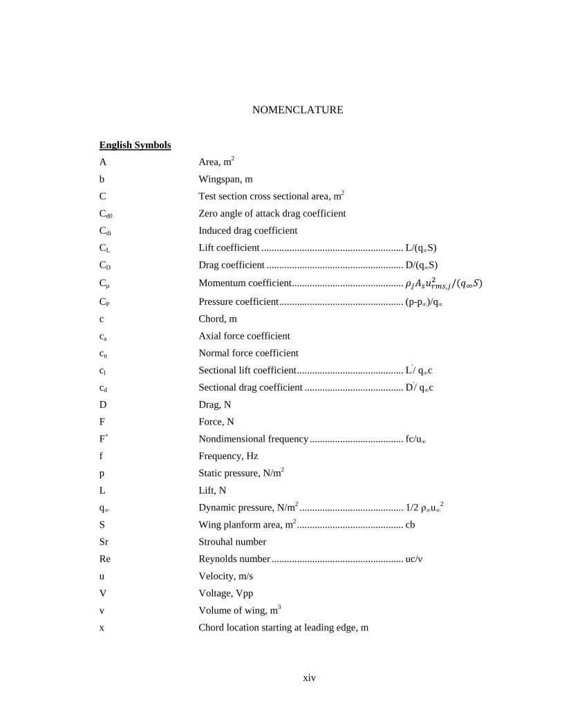
NOMENCLATURE
English Symbols
A Area, m2
b Wingspan, m
C Test section cross sectional area, m2
Cd0 Zero angle of attack drag coefficient
Cdi Induced drag coefficient
CL Lift coefficient ........................................................ L/(q∞S)
CD Drag coefficient ...................................................... D/(q∞S)
Cµ Momentum coefficient ............................................
CP Pressure coefficient ................................................. (p-p∞)/q∞
c Chord, m
ca Axial force coefficient
cn Normal force coefficient
cl Sectional lift coefficient .......................................... L'/ q∞c
cd Sectional drag coefficient ....................................... D'/ q∞c
D Drag, N
F Force, N
F+ Nondimensional frequency ..................................... fc/u∞
f Frequency, Hz
p Static pressure, N/m2
L Lift, N
q∞ Dynamic pressure, N/m2 ......................................... 1/2 ρ∞u∞
2
S Wing planform area, m2 .......................................... cb
Sr Strouhal number
Re Reynolds number .................................................... uc/ν
u Velocity, m/s
V Voltage, Vpp
v Volume of wing, m3
x Chord location starting at leading edge, m

xv
Greek Symbols
α Angle of Attack, deg
ρ density, kg/m3
Subscripts
A Actual
af Airfoil
B Buoyancy
i An index
j Jet
p Static Pressure
q Dynamic Pressure
RMS Root mean squared
s Slit
sb Solid blockage
t Total
tot Total
wb Wake Blockage
ε Blockage
∞ Freestream
Acronyms
SJA Synthetic Jet Actuation
SJ Synthetic Jet
AFC Active Flow Control
PFC Passive Flow Control
FSO Full Scale Output
CFD Computational Fluid Dynamics

1
1 Introduction
With today’s rising fuel prices, aircraft designers are looking for new ways to reduce the
fuel consumption of aircraft. Reducing an aircraft’s drag is one way to do this. It was estimated
that a drag reduction of 10% on a single typical subsonic military aircraft would save 13 million
gallons of fuel throughout its design life1. Various efforts have been geared towards achieving
such drag reductions with a portion of these efforts focusing on wingtip devices. A properly
designed wingtip device can modify a wing’s lift distribution in a way that causes the wing to
produce lift more efficiently. This improved efficiency decreases the lift-induced drag on the
aircraft. Reducing the induced drag, which in certain cases accounts for about 30 percent of total
drag for cruise2 and 80-90 percent for takeoff and landing
3, would reduce the fuel consumption
and could significantly reduce aircraft operating cost. In addition to reducing the induced drag,
wingtip devices may have secondary benefits such as reducing the wake vortex hazard to trialing
aircraft by weakening the trialing vortex4, and reducing carbon emissions by lowering fuel
consumption5.
This document describes the wind tunnel test of an active “wingtip device” integrated into a
NACA 0015 semispan model. This newly developed device uses an array of 8 piezoelectric disk
actuators combined in series to create a synthetic jet that emanates out of the wingtip. It is
believed that this synthetic jet device can be used to reduce the induced drag on a wing.
1.1 Literature Survey
The idea of a “wingtip device” to reduce induced drag has been around since the early 20th
century. Whitcomb, who coined the term winglet, seems to be the first to realize the potential
induced drag benefits of these devices6. There have been several other winglet designs since
then, notably the A310 tip fence, tip sails, and the vortex diffuser7. Although these devices
generally provide a decrease in induced drag when designed correctly, they oftentimes do not

2
“buy their way” onto aircraft. Reasons include structural issues, weight penalties, poor off design
performance, and a net increase in other drag components such as profile drag8.
Active flow control (AFC) is being researched as an alternative and can eliminate many of
the drawbacks associated with winglets. One benefit of AFC is that it is more versatile than
passive flow control (PFC). This is because active devices can be scaled, turned on and off, and
optimized throughout the flight envelope while passive devices cannot be modified as much and
are generally optimized for one flight condition. Most AFC devices also have a minimal drag
penalty since they are generally placed inside or near the wing surface. An early and widely
studied wingtip AFC method involves steady blowing in the spanwise direction outboard from
the wingtip. This generally results in an effective increase in span pushing the vortices outboard
and diffusing the vortex. The diffused and displaced vortex produces a smaller downwash leading
to an increase in lift and a decrease in induced drag for long-chord jets9. One issue with steady
blowing AFC technology is that it requires a complicated ducting system to provide actuation. In
addition, steady blowing has been shown to be impractical as the input required is greater than the
increase in aerodynamic efficiency9. Synthetic jet or zero-net-mass-flux (ZNMF) actuation
eliminates the ducting issue, as no air supply is needed. Studies have also shown that synthetic
jets work better than steady blowing for separation control10
and that a synthetic jet entrains more
fluid than a continuous jet11
. This could mean that lower input is needed for a synthetic jet to
achieve the same control authority and may prove synthetic jets more practical than steady
actuation.
Limited research has been performed on the use of synthetic jets to control wingtip vortices
although one study reported that synthetic jet actuation diffuses the vortex reducing core voritcity
and maximum tangential velocity12
. The paper compared the effect of synthetic jet actuation to
the effect of steady blowing. Synthetic jet actuation and steady blowing showed similar effects
for lower momentum coefficients but the synthetic jet shows a significantly more diffuse vortex

3
for higher momentum coefficients. Recently, plasma actuation has been used to control the
wingtip vortex providing promising results13,14
. In a CFD simulation, a dielectric barrier discharge
(DBD) actuator was able to block the crossflow around the wingtip at the origin of the vortex
formation to produce a diffused vortex, decreased downwash, and a 20% increase in lift.
Although promising, DBD actuators powerful enough to have these effects are still in
development. Synthetic jets on the other hand have been shown to experimentally produce
adequate excitation.
1.2 Purpose
The goal of this study is to conduct an experiment to determine if synthetic jet actuation is
effective for reducing the induced drag on a finite wing. This study will expand on previous
work12
which showed the effect of synthetic jet actuation at several locations at the wingtip via
particle image velocimetry (PIV). This previous paper concluded that synthetic jet actuation
produces a diffuse vortex although did not provide any direct information about drag. The current
study will conduct a similar experiment, using the most effective slit location from the previous
study, and will provide direct drag measurements. This study will also test a wider range of angle
of attack, Cµ, and Reynolds number. A CD vs CL2 curve will be plotted with and without
actuation to see if actuation has any effect on the induced drag. Several supporting data sets will
be attained as well. Pressure data will be obtained through several pressure ports embedded in the
model. This will be used to see if actuation is causing the lift coefficient to change near the
wingtip as a change in the lift distribution should affect the induced drag. Oil droplet flow
visualization will also be performed to see how actuation affects the local flowfield near the
wingtip. Several things need to be completed to perform this study. First, a synthetic jet actuator
needs to be designed and built that is suitable for active flow control. This actuator will need to be
tested to ensure it provides sufficient actuation. Second, a compact semispan wing will have to be
built which can contain these actuators and can fit inside the Cal Poly 2x2 ft. subsonic wind

4
tunnel. Sensors will have to be integrated into the model to measure drag and see if any decrease
in induced drag is present. One requirement of the model is that it needs to be able to provide
suction surface as well as tip actuation. This is because the model will be used for two different
Thesis’ (more information on this in section 4). Tip actuation will be used for this Thesis. Finally,
the model will be tested in a wind tunnel to see if synthetic jet actuation from the wingtip
provides any reduction in induced drag.
In summary, the goals of the current study are:
1. Design, build, and test a synthetic jet actuator
2. Design and build a NACA 0015 semispan wing model containing synthetic jet actuators
that can provide suction surface, spanwise tip actuation, and a way to measure drag.
3. Expand upon a previous effort12
to control wingtip vortices via synthetic jet actuators.
This will be done by conducting a wind tunnel experiment using the NACA 0015
semispan model with synthetic jet actuation at the wingtip, measuring the induced drag,
and providing conclusions about the effect of synthetic jet actuation on induced drag.
5
1.3 Background
1.3.1 Wing Tip Vortices
Tip vortices are formed at the terminating end of any lifting surface. They cause the air
behind the lifting surface to swirl in a circular motion. Wingtip vortices, which form at the tips of
aircraft wings, are the most notable occurrence of this and are widely researched by
aerodynamicists, as they are detrimental to the aerodynamic efficiency of aircraft. Researchers
often attempt to weaken, diffuse, or push these vortices outboard to reduce their effect on
aerodynamic efficiency. Understanding the formation of the wingtip vortex is important in any
effort to control it.
Green gives three distinctive and complimentary explanations for the occurrence of wingtip
vortices15
. The first and simplest method involves the pressure differential between the top and
bottom wing surfaces. Due to the nature of the flow around a wing, the pressure on the upper
(suction) surface is lower than the pressure on the lower (pressure) surface. This pressure
differential accelerates the flow around the wingtip from the pressure surface to the suction
surface combining with the streamwise velocity component creating a wingtip vortex. The
second explanation involves the shear layer that exists near the wingtip. The freestream flow and
the flow over the wing are not parallel which implies voritcity approaching the wing tips. This
mechanism allows for the production of wingtip vortices of opposite sign on each side of the
wing even without the production of lift, which actually does occur experimentally16
. The third
explanation involves the Helmholtz vortex laws. Here, the wingtip vortex is presented as a
connection between the starting vortex and the bound vortex since vortex lines can never end in a
fluid.
A more recent paper indicated that flow over the wingtip is more complicated, involving
many different phenomena such as the interaction of multiple vortices, multiple separations and
attachments, as well as being highly dependent on the wing geometry16
. This paper contained
6
flow over a square, untapered, and untwisted NACA 0012 wingtip (a square NACA 0015 is
tested in this thesis) showing the formation of four vortices. These vortices eventually interact
forming a highly unsteady vortex system that includes several secondary vortices.
1.3.2 Lift-Induced Drag
Induced drag is often the referred to as the price for producing lift. A basic way to
understand induced drag is that the flow around the wingtip, aka wingtip vortex, contains a lot of
translational and kinetic energy, which is wasted when the vortex is shed off the airplane. The
engine has to work harder to overcome this wasted energy, hence to overcome the induced drag.
A more systematic way to understand induced drag is as follows. The vortices shed from each tip
create downwash or a downward velocity component ahead of the wing. This combines with the
freestream velocity creating a local velocity around the wing that is canted downward. The local
lift vector adjusts accordingly to be perpendicular to the local velocity producing a lift vector
component in the freestream direction. This component can be thought of as the induced drag.
According to Prandle’s classical lifting-line theory the induced drag is proportional to the lift
squared and inversely proportional to the aspect ratio. Therefore, according to this theory, the
induced drag can be reduced by increasing the span or changing the lift on the wing.
1.3.3 Zero-Net Mass-Flux Actuators
A zero-net mass-flux actuator commonly known as the “synthetic jet” is formed by the
periodic expulsion and ingestion of a fluid through an orifice. It is called a synthetic jet because
there the jet is made or “synthesized” from the surrounding fluid. It ingests low speed fluid and
ejects it at a higher speed adding momentum to the flow without adding mass. Synthetic jet
actuators are commonly used for flow control applications, including separation control, mixing
control, and combustion control to name a few. The most common synthetic jet actuator
assemblies are piston cylinder, voice-coil magnet, or piezoelectric disk. The controlling
7
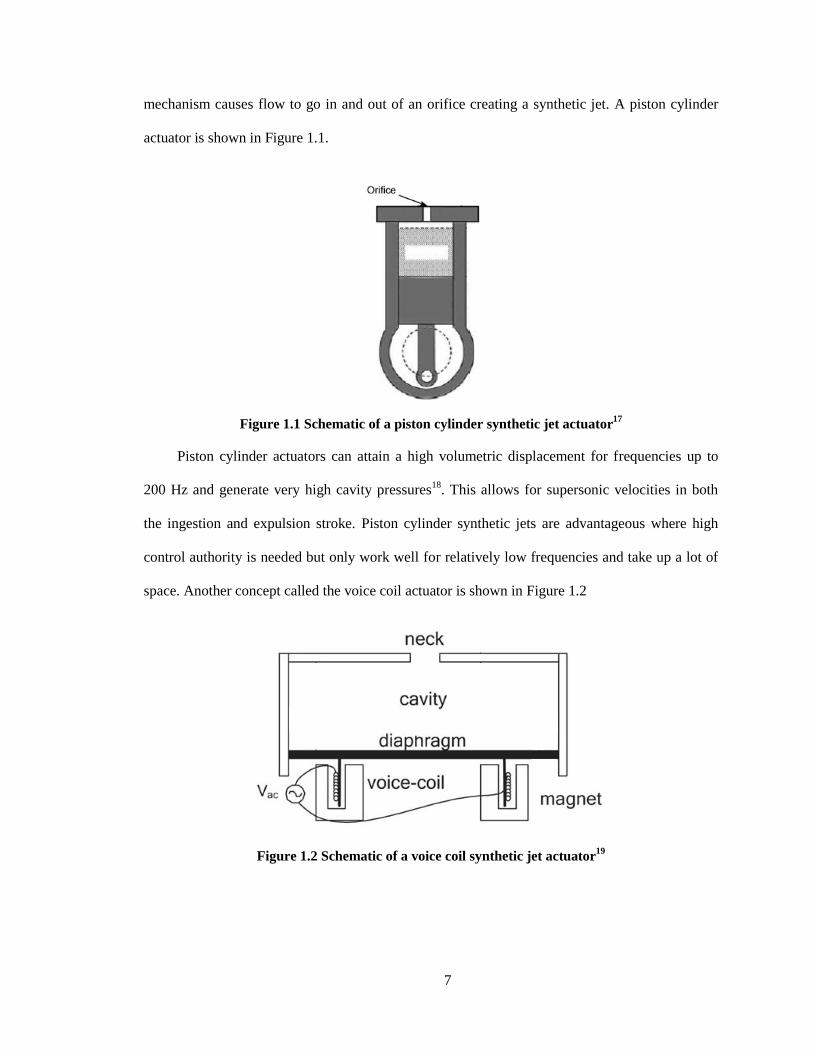
mechanism causes flow to go in and out of an orifice creating a synthetic jet. A piston cylinder
actuator is shown in Figure 1.1.
Figure 1.1 Schematic of a piston cylinder synthetic jet actuator17
Piston cylinder actuators can attain a high volumetric displacement for frequencies up to
200 Hz and generate very high cavity pressures18
. This allows for supersonic velocities in both
the ingestion and expulsion stroke. Piston cylinder synthetic jets are advantageous where high
control authority is needed but only work well for relatively low frequencies and take up a lot of
space. Another concept called the voice coil actuator is shown in Figure 1.2
Figure 1.2 Schematic of a voice coil synthetic jet actuator19

8
The voice coil actuator is essentially a speaker attached to a cavity. It is capable of high
frequency actuation and has a higher control authority than a piezoelectric synthetic jet but it is
not as compact. A piezoelectric synthetic jet is shown in Figure 1.3.
Figure 1.3 Schematic of a piezoelectric synthetic jet actuator20
The piezoelectric synthetic jet actuator is the simplest actuator of three. It consists of a
piezoelectric disk, which acts as a diaphragm, and a cavity with a small orifice. Electric leads are
attached to the disk on each side and an A/C current makes the disk oscillate forcing air in and
out of the orifice. Although the piezoelectric synthetic jet has the lowest control authority, it is the
easiest to build and is the most compact.
1.3.4 Momentum Coefficient
The momentum coefficient is a nondimensional parameter used to characterize the output of
a flow control actuator. It is a common parameter in flow control studies and is used to gauge the
effect of actuation on the performance parameters of interest. It is often defined by a steady
component and an unsteady component.
1.1
For example, a synthetic jet would be defined purely by the unsteady component while
steady blowing would be defined by the steady component. There are also schemes that use

9
pulsed control, which would superimpose a steady mass flux into onto a zero-net-mass-flux
device. This would be defined by both the steady and unsteady components. In this paper only the
unsteady momentum coefficient is used which can be defined as:
1.2
Some papers use the peak jet velocity and some papers use the root mean squared (RMS) jet
velocity for synthetic jets. There is also some discrepancy in how the RMS velocity is calculated.
The RMS velocity can be calculated by using the velocity profile of the entire synthetic jet cycle
(expulsion and ingestion) or just from the expulsion portion. This study uses the RMS velocity of
the expulsion phase.
1.3.5 Non-Dimensional Frequency, F+
F+ is a non-dimensional frequency describing oscillating flow mechanisms. It is the ratio of
the time it takes flow to travel over the wing to the characteristic period of the actuator.
1.3
In vortex control, F+ is sometimes termed Strouhal Number and is used to measure
phenomena such as vortex meandering, vortex instabilities, and shear layer instabilities.

10
2 Design and Manufacture of Experiment
Synthetic jet actuators and an AFC test apparatus were not readily available for use. A
preexisting AFC test apparatus would have to be bought from an independent source, which
would be beyond the budget of this experiment. It was much more feasible to build the apparatus
from scratch. The complexity and precision needed for the design were too high to do by hand.
Therefore, everything was built using automated machinery
The design philosophy was to design for manufacturability. It was necessary to keep things
as simple as possible because any added complexity leads to more difficulty in manufacturing.
Because manufacturing is much more time consuming than the design process, essentially this
philosophy reduces the time it takes to build everything.
2.1 Manufacturing Equipment
All of the manufacturing was done in the Cal Poly Mustang 60 machine shop, the Cal Poly
Hangar, and the Cal Poly Aerospace Department’s machine shop. It was necessary to receive the
Blue tag certification from the Mustang 60 machine shop in order to be able to use the CNC
machinery in this section. The prerequisites for this certification were 60 hours of logged shop
use, taking a tour and passing a written test, and completion of a guided CNC project on each
machine that would be used. The machines used for manufacturing this experiment are discussed
in the following sections
2.1.1 Haas VF-3
The Haas VF3 is a CNC vertical milling center with a 40" x 20" x 25" travel. More specifics
about the machine can be found at the Haas website. This is the only machine available on
campus that was large enough to machine the NACA 0015 model. A picture of the VF-3 is shown
in Figure 2.1

11
Figure 2.1 Haas VF-3
This machine has several upgrades that made it more convenient to machine the NACA
0015 including: a 15,000-rpm Spindle, a Side-Mount Tool Changer, a Chip Auger, and Wireless
Intuitive Probing System (shown in Figure 2.2). A high-speed spindle was effective at reducing
the already high 32 hour run time. A side-mount tool changer was necessary because a standard
tool holder could not hold the 15 tools that were used for machining. The chip auger was coded to
turn on automatically every hour of machining to remove chips and prevent them from clogging
the coolant filtration system.
Figure 2.2 Wireless Probing System: Tool Setter (left) and Wireless Probe (right)
The wireless probing system was used as a quick and efficient way to set tool and part
offsets and was very useful to reduce the setup time. The wireless probe would be used to touch
off on the NACA 0015 giving the machine a reference of where the part is located relative to the

12
spindle. Then, each tool would be touched off on the tool setter measuring its z-distance relative
to the top of the NACA0015. The g-code for this machine was created using CAMWorks.
2.1.2 Haas Super Minimill 2
The Haas Super Minimill 2 is a CNC vertical milling center with a 20" x 16" x 14"travel,
shown in Figure 2.3. More specifics about the machine can be found at the Haas website. This
machine is smaller, easier to manage, and easier to clean than the VF-3. The VF-3 can do
everything this machine can although it was much more convenient to work in this machine. The
Minimill was used to build the smaller parts including the synthetic jet actuator, the wingtip, and
some of the supporting structure. The VF-3 and the Minimill were often used simultaneously. The
VF-3 would be machining large parts that take a long time. During this wait period, several small
components could be machined on the Minimill. The mini also had similar upgrades to the VF-3
including the Wireless Intuitive Probing System. The g-code for this machine was created using
CAMWorks
Figure 2.3 Haas Super Minimill 2
2.1.3 Haas TL-1
The Haas TL-1, shown in Figure 2.4, is a CNC/Manual Toolroom Lathe with a 16" x 29"
max capacity. More specifics about the machine can be found at the Haas website. Several
cylindrical components of the experimental apparatus had to be cut to precise lengths, drilled, and

13
tapped. This machine was ideal for machining these components as it could be programmed to do
these features automatically. The g-code for this machine was generated using the quick-code
feature where simple operations such as drilling and tapping could be set using the TL-1 user
interface.
Figure 2.4 Haas TL-1
2.1.4 Universal Laser Systems VLS6.60 Laser cutter
The VLS6.60 laser cutter shown in Figure 2.5 is a high-powered laser used for cutting or
engraving material. This laser uses a high power density allowing the laser to be focused on a
very small spot for precision cutting and can cut objects up to 37 x 23 x 9 in. This laser cutter was
used to cut gaskets for the actuator. It was necessary to have a thin, narrow, nonconductive gasket
of specific dimensions to minimize the clamping area and insulate the piezoelectric disk. A gasket
like this could not be purchased. The laser cutter proved efficient for cutting the delicate neoprene
gasket material precisely.

14
Figure 2.5 Universal Laser Systems VLS6.60 Laser Cutter
2.2 Synthetic Jet Actuator
In order to conduct the active flow control experiment, a synthetic jet actuator needed to be
built. Several actuator concepts were considered (see section 1.3.3) but it all came down to
getting the apparatus to fit inside the Cal Poly 2x2 wind tunnel and the piezoelectric actuator was
chosen due to its compactness. Several types of piezoelectric materials were considered based on
which could provide the highest peak velocity. A study was found which showed peak velocities
for three materials using three different wave types21
. Results of the study are shown in Table 2.1
Table 2.1 Peak jet velocities (m/s)21
From this, it can be seen that the Bimorph actuator produces the highest velocity output and
that a square wave is the best driving signal. Another study was found which experimentally
derived a model for the velocity of a Bimorph actuator22
. This model is shown in equation 2.1.
2.1
Diaphragm Waveform
Sine Saw-tooth Square
Bimorph 7 ± 2 35 ± 6 36 ± 5
Thunder 5 ± 2 26 ± 2 27 ± 2
RFD 6 ± 2 28 ± 2 32 ± 2
15
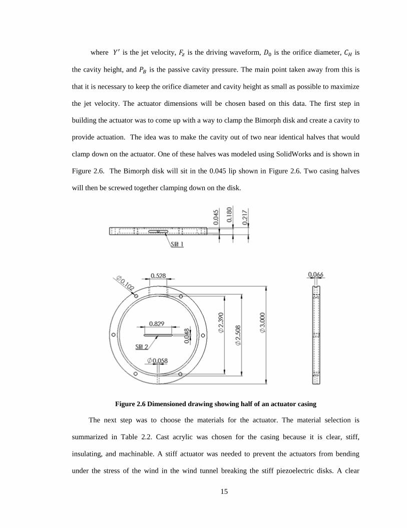
where is the jet velocity, is the driving waveform, is the orifice diameter, is
the cavity height, and is the passive cavity pressure. The main point taken away from this is
that it is necessary to keep the orifice diameter and cavity height as small as possible to maximize
the jet velocity. The actuator dimensions will be chosen based on this data. The first step in
building the actuator was to come up with a way to clamp the Bimorph disk and create a cavity to
provide actuation. The idea was to make the cavity out of two near identical halves that would
clamp down on the actuator. One of these halves was modeled using SolidWorks and is shown in
Figure 2.6. The Bimorph disk will sit in the 0.045 lip shown in Figure 2.6. Two casing halves
will then be screwed together clamping down on the disk.
Figure 2.6 Dimensioned drawing showing half of an actuator casing
The next step was to choose the materials for the actuator. The material selection is
summarized in Table 2.2. Cast acrylic was chosen for the casing because it is clear, stiff,
insulating, and machinable. A stiff actuator was needed to prevent the actuators from bending
under the stress of the wind in the wind tunnel breaking the stiff piezoelectric disks. A clear

16
actuator was necessary to do quick visual damage assessments for things such as broken disks or
disconnected leads. A maximum of 180 volts and 200 mA would be applied to the actuator so the
electric insulation property was crucial for safety reasons. In addition, this actuator needed to be
machined and acrylic is very machinable. The Bimorph material was chosen due to its velocity
output as showed previously in this section. A gasket was necessary to provide a cushion for the
Bimorph protecting it from being damaged as the casings clamp together on the disk’s outer edge.
Machine screws are used to clamp the actuator together. The electric leads are needed provide
power to the actuator. The thinnest flexible wire that could handle 180 volts and 200 mA was
used to prevent strain on the disk that could damage the actuator during operation.
Table 2.2 Actuator Materials
This casing was then manufactured using a Haas Minimill. The tools, tool paths, feeds, and
speeds were all set using CAMWorks, which converted them to G-code to be read by the VF2.
The piece of acrylic was squared off manually and then fixtured using a vise. A Haas Renishaw
Probe was used to set the part offsets. A Haas wireless tool setter was used to set the tool lengths.
The gasket also had to be manufactured. A sketch of the gasket was made using Adobe
Illustrator which was then printed to a Universal Laser Systems VLS6.60 Laser cutter. A Power
of 55%, speed of 10%, and pulses per inch (PPI) of 600 were the laser settings used for cutting
the gasket. In addition, the gasket was cut a bit larger than showed in Table 2.2 to account for the
Part Material
Casing Cast Acrylic
Actuator Bimorph, Piezo Systems part no.
T216-A4NO-573X
Gasket 0.032” in thick 2.508 OD 2.390 ID
neoprene
Machine Screws ¼ 5-40, Stainless Steel
Electric Leads Continuous-Flex Miniature Wire 26 AWG

17
laser diameter. The actual OD and ID that were commanded to the laser are 2.512” and 2.386”
respectively. Figure 2.7 shows the complete and assembled actuator. For the initial tests,
electrical tape was used to hold the leads in place. Later on, the leads were soldered to the disk.
Figure 2.7 Assembled synthetic jet actuator
It was necessary to measure the velocity output of the actuator to get an estimate of Cµ for
use in the design of the NACA 0015 model. Slit 1 and slit 2 (shown in Figure 2.6) were tested
because they were thought to represent the slit orientations used in the NACA 0015 model (see
Section 2.3). The peak and RMS velocity profiles for each slit orientation are shown in Figure
2.8.

18
Figure 2.8 Peak and RMS velocities for Slit 1 and 2
The velocity profiles for slits 1 and 2 are not drastically different. This means that velocities
of this magnitude may be expected when the actuators are mounted in the model.
2.3 NACA 0015 Semispan Model
A major effort in this thesis was the design and manufacture of the NACA 0015 Semispan
model. The goal was to keep the design as simple as possible so avoid overcomplicating the
manufacturing process. The first step in the design was to figure out the size of the model. The
NACA 0015 airfoil was chosen because this was the airfoil used in the previous study. The chord
of the model needed to be as small as possible to prevent wind tunnel blockage and to increase
Cµ. The problem with decreasing the chord too much was that the actuators and pressure ports
could not fit if the chord was too small. After some initial SolidWorks design, a chord of 8 inches
was found to be enough to fit the actuators and pressure ports (a detailed SolidWorks drawing
will be shown later in this section). Wind tunnel blockage corrections will be used to offset the
blockage effect. It was necessary to prove that the synthetic jet actuator could provide sufficient
actuation for a wing with an 8-inch chord. For this study, a Cµ of 0.0008 was needed to match the

19
experiment in reference 12. Figure 2.9 contains an estimate of Cµ for an 8-inch chord with
spanwise SJA (synthetic jet actuation) showing that the actuators should be strong enough for this
experiment.
Figure 2.9 Cµ estimate for spanwise actuation
The momentum coefficient was obtained using the peak velocity data from slit 1 in Figure
2.8. The velocity was corrected using conservation of momentum to represent the actual slit that
will be used in the experiment. The estimated momentum coefficient varies from about 0.0003 to
0.0052. After 40 Hz, the estimated value is higher than the largest Cµ of 0.0008 used in the
previous study meaning an 8-inch chord wing could be used. The span of the model was 23
inches. Although this value is larger than needed for the 2”x2” tunnel, the model was designed so
it could be retracted under the tunnel reducing the effective span.
Now that the size of the wing was set, it was necessary to figure out the overall layout of the
wing. A key characteristic that made it possible to create a compact model was the idea of turning
one synthetic jet actuator disk into two synthetic jet actuators by using the same actuators for

20
suction surface and spanwise actuation. A schematic showing this concept is shown in Figure
2.10.
Figure 2.10 Dual synthetic jet concept
Using two cavities, less energy is used for actuation and two jets are produced instead of
one. The vertical jet would be used for suction surface actuation and the horizontal jet would be
used for spanwise (wing tip) actuation. This concept was expanded by combining several
actuators to get one stronger jet since only one jet was needed for spanwise actuation. A
schematic of this idea is shown in Figure 2.11.
Figure 2.11 Combined actuator concept
The vertical arrows represent suction surface actuation and the horizontal arrow represents
spanwise actuation. The layout of the wing was built around this concept. The top half of the
wing would be used as half an actuator case providing suction surface actuation and the bottom of
the wing would be used as half an actuator case providing spanwise actuation. A wingtip would
be built in order to channel the spanwise actuation into a slit that has similar dimensions to the slit
used in the previous study.

21
The pressure port layout was chosen next. The placement of the pressure ports was effected
by a few factors. First, manufacturing constrains made it so that only a certain number of pressure
ports could be fit in a given area. In addition, room needed to be made for pressure tubing since it
would need to run out of the model and into the RAD3200 System. Second, a study that would be
performed by another student needed to sense separation and assess the effect of suction surface
actuation along the span. Therefore, pressure ports needed to be spread out in rows along the span
and pressure ports were needed near the trailing edge to sense separation. Lastly, pressure ports
were needed near the wingtip to see if spanwise actuation had significant effect at the wingtip.
The pressure port layout is shown in Figure 2.12
Figure 2.12 Pressure port row locations
The 2y/b locations for the rows A, C, D, and F are 37.5%, 70.2%, 85.1%, and 93.1%
respectively. The 2y/b locations for rows B and E are 37.5 and 85.1 respectively. More rows were
placed on the suction surface than the pressure surface. This is because the other study was more
interested about how suction surface actuation affects the pressure distribution on the suction
surface than how it affects the distribution on the pressure surface. The pressure port x/c locations
for rows A, C, D, and F are shown in Table 2.3 and the x/c locations for rows B and E are shown
in Table 2.4.
0.0 5.1 10.2 15.2 20.3 0.0
16.0
29.6
36.4
39.7
42.7
x [cm]
y [cm
]
Suction Surface
Row A
Row C
Row D
Row F
0.0 5.1 10.2 15.2 20.3 0.0
16.0
36.4
42.7
x [cm]
y [cm
]
Pressure Surface
Row B
Row E

22
The pressure ports were clustered near the front of the wing to capture the large pressure
gradients at the leading edge. Pressure port 4 in row A was non-functional due to damage caused
during manufacturing and will not be used in this experiment.
The next step in the design process was to choose the materials for each part of the model.
The wing material needed to have several qualities. First, it had to be machinable. The machining
process would take many hours and require the use of many small specialty end mills. If the
material were something tough or abrasive, end mills would have a very short lifecycle. A
machining time estimation by CAMWorks showed that the setup will take at least 8 hours to
machine. For machining operations this long, the machine is generally run overnight. If an end
mill breaks during this process, the machine would continue running and it would affect the next
milling feature most likely breaking that end mill too. This would lead to many broken end mills
and an unfinished part. This whole problem could be avoided by choosing an easily machinable
material. The next consideration was stiffness. A stiff material was needed so it does not deflect
under aerodynamic forces and break the stiff actuators. A material was also needed that did not
conduct electricity because 180 Vpp would be supplied to each actuator providing a current of up
to 200 mA. If the wing was conductive and the model was touched while the actuators were one,
Table 2.3 Top pressure port locations
Port # x/c [%]
1 0.2
2 0.5
3 1.3
4 2.1
5 4.7
6 10.0
7 20.0
8 30.0
9 45.0
10 60.0
11 90.0
Table 2.4 Bottom pressure port locations
Port # x/c [%]
1 1.0
2 2.0
3 5.2
4 10.0
5 20.0
6 40.0
7 60.0
8 90.0

23
the user could be shocked by the high voltage and current. With all of these factors taken into
hand, materials considered were wood, plastic, and ceramic. Wood was discarded because
inconsistencies in grain can create gaps creating leaks in the actuators, also wood clogs coolant
filters for the milling machines. Machinable ceramic (MACOR) was eliminated because even
though it is labeled as “machinable” it is very abrasive and causes tools to wear very quickly.
This was not acceptable for an 8 hour operation. It is also very brittle and a light bump can shatter
it. Plastic seemed like the best choice. Several plastics were considered but polycarbonate and
acrylic were favorable because they are clear. It would be easy to assess the condition of the
model (e.g. actuator damage) with the structure being clear. Polycarbonate is more machinable
and much less brittle but is it is also less stiff. It was thought that the polycarbonate would be too
flexible and break the actuators under aerodynamic forces. Therefore, acrylic was chosen for the
wing structure. The wing spars were initially of aluminum construction to reduce the weight of
the assembly but after testing, it was realized that aluminum is too flexible and a steel spar was
made.
Now that the size, material, overall layout, and pressure port locations are set, the wing was
designed in SolidWorks so it could be manufactured. The top half of the wing is shown in Figure
2.13

24
Figure 2.13 Top half of the wing showing internal details
The top half of the wing was designed so it could be built out of one piece of material using
three mill part setups. It will have lateral and longitudinal steel spars to prevent it from snapping
in half in the wind tunnel, eight casings for actuators with room between each case for ducting,
and a male fitting on which the wingtip will be placed. Near the tip of the wing, the leading edge
has material removed to make room for pressure ports. Most of the pressure port holes were
designed to be drilled on the CNC although near the leading edge this was impossible due to the
high curvature. Near the leading edge 0.01” holes at a 0.005” depth were added. These would
serve as markings to where the leading edge pressure ports are to be and drilled by hand. A 0.01”
endmill would be used to make these markings on the CNC. Screw holes were added on both
sides of the longitudinal spar. On the leading edge side the screw held a dual purpose of holding
the two wing halves together as well as clamping the actuators together. A 2.130 x 0.039” slit was
cut at a 30 degree angle from the surface of the wing in each actuator at 10% chord for another
study. Choosing to cut the slit at a 1mm (0.039”) width and a 30 degree angle involved careful
consideration. The student doing the separation control study needed a slit no greater than 0.039”

25
cut at as small of an angle to the surface as possible so the jet is blowing downstream. It was
necessary to find an endmill that could make this cut. From previous experience machining the
synthetic jet, the thinnest possible actuator cavity ceiling thickness was 0.04”. Any thinner and
the acrylic would warp from machining and could even crack. Therefore, if cutting perpendicular
to the surface (ϴ = 90 degrees, where ϴ is the angle of the cutter relative to the surface), the flute
length of the endmill would need to be 0.04”. As the slit angle decreases the flute length needed
to make the cut increases with 1/cos(ϴ). Since endmills have a direct relationship between max
flute length that can be manufactured per endmill and endmill diamter, a larger endmill would
make it easier to cut at a smaller angle. Therefore, the maximum allowed slit width of 1 mm was
chosen. The next issue was choosing the angle to cut. One constraint was that it is harder to get a
CNC mill chuck close enough to the surface of the wing as you decrease the slit angle because
you have to fixture the model at an angle to make the cut. Another constraint is that the maximum
flute length for readily available 1 mm endmills is 4mm. After considering these geometric
constraints, it was found that a 30 degree slit could be cut.
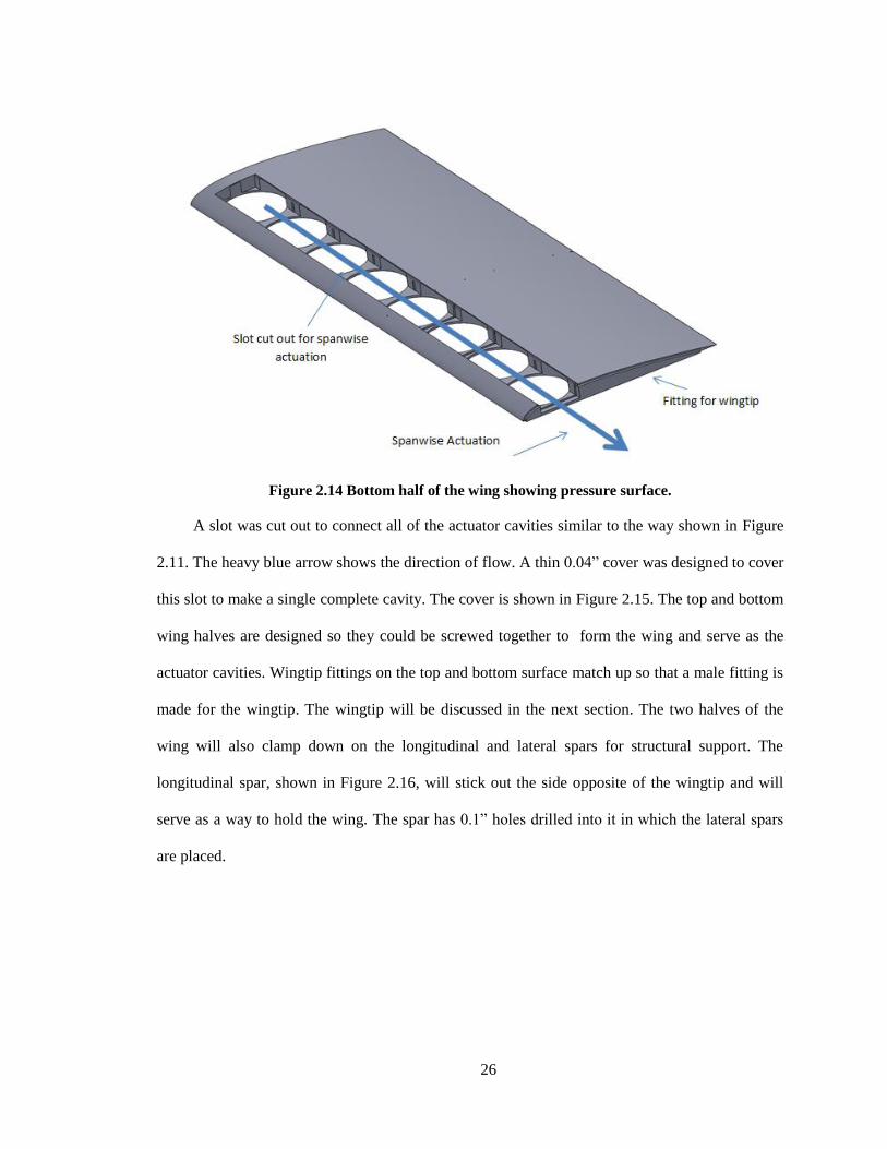
The next part to be designed was the bottom surface of the wing, shown in Figure 2.14. The
pressure surface is shown in thise view (the internal sturctre is not shown because it is almost
exactly the same as in the top half shown in Figure 2.13).
26
Figure 2.14 Bottom half of the wing showing pressure surface.
A slot was cut out to connect all of the actuator cavities similar to the way shown in Figure
2.11. The heavy blue arrow shows the direction of flow. A thin 0.04” cover was designed to cover
this slot to make a single complete cavity. The cover is shown in Figure 2.15. The top and bottom
wing halves are designed so they could be screwed together to form the wing and serve as the
actuator cavities. Wingtip fittings on the top and bottom surface match up so that a male fitting is
made for the wingtip. The wingtip will be discussed in the next section. The two halves of the
wing will also clamp down on the longitudinal and lateral spars for structural support. The
longitudinal spar, shown in Figure 2.16, will stick out the side opposite of the wingtip and will
serve as a way to hold the wing. The spar has 0.1” holes drilled into it in which the lateral spars
are placed.

27
Figure 2.15 Pressure surface actuator cover
Figure 2.16 Wing longitudinal spar
The lateral spars are steel rods with a 0.1” diameter and prevent the wing from shearing due
to the moment caused by aerodynamic loads. They also prevent the wing from sliding down the
longitudinal spar. The holes were placed every 0.667” to allow to model to be raised by 0.667”
inches if necessary. 0.667” was chosen because the lateral spars slots could only be placed
between the actuators and 0.667” is a quarter the distance between actuators, allowing for an even
hole spacing.
The last part of the wing design was the wingtip. The wingtip has to fit on the fitting created
by the both halves of the wing and the cover. The wingtip also needs internal ducting to direct the
flow from spanwise actuation to the slit. Figure 2.17 shows the wingtip as if looking into the y-
axis of the wing.
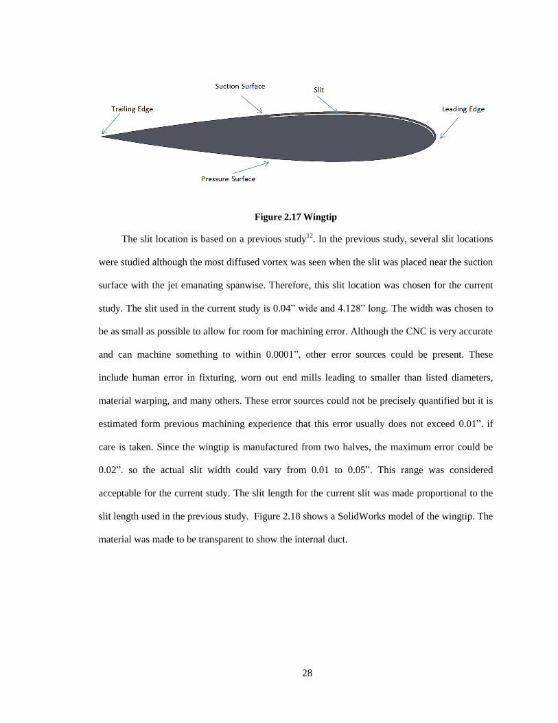
28
Figure 2.17 Wingtip
The slit location is based on a previous study12
. In the previous study, several slit locations
were studied although the most diffused vortex was seen when the slit was placed near the suction
surface with the jet emanating spanwise. Therefore, this slit location was chosen for the current
study. The slit used in the current study is 0.04” wide and 4.128” long. The width was chosen to
be as small as possible to allow for room for machining error. Although the CNC is very accurate
and can machine something to within 0.0001”, other error sources could be present. These
include human error in fixturing, worn out end mills leading to smaller than listed diameters,
material warping, and many others. These error sources could not be precisely quantified but it is
estimated form previous machining experience that this error usually does not exceed 0.01”. if
care is taken. Since the wingtip is manufactured from two halves, the maximum error could be
0.02”. so the actual slit width could vary from 0.01 to 0.05”. This range was considered
acceptable for the current study. The slit length for the current slit was made proportional to the
slit length used in the previous study. Figure 2.18 shows a SolidWorks model of the wingtip. The
material was made to be transparent to show the internal duct.

29
Figure 2.18 Wingtip
The flow from the bottom wing half travels into the flow entrance and is channeled through
the internal duct. The flow exits the internal duct from the slit providing spanwise actuation out of
the wingtip. This wingtip design is impossible to manufacture using a 3 axis CNC milling
machine in the single-piece configuration shown. This was considered and the wingtip was
therefore designed so it could be built in two halves which can be glued together to produce the
configuration shown in Figure 2.18. These halves are shown in Figure 2.19
Figure 2.19 Wingtip halves
Now that each piece of the wing was designed and modeled in SolidWorks, the wing could
be manufactured.

30
The first step of the machining process was to create the g-code code for the CNC
machines. CAMWorks is a software that makes this a seamless process. Using CAMWorks, each
feature on each of the solid models was converted into a milling operation. These milling
operations consist of toolpaths that the user defines and customizes by changing various operation
parameters. The higher-level parameters are, milling speeds and feeds, end mill diameters, and
depth of cuts but many more exist. CAMWorks converts all of this information into g-code,
which is that language that the CNC reads. An example of one of these toolpaths is shown in
Figure 2.20. The blue line is the path the center of the end mill will follow during machining. The
toolpaths were simulated once all of the operations were finalized as shown in Figure 2.21.
Simulating the toolpath serves as a safety check since the toolpath is simulated exactly as the
CNC will machine the feature showing the end mill and the original stock. The simulation shows
if the CNC will create unwanted cuts or leave uncut material in certain places. The screenshot
shown in Figure 2.21 shows the machining of the lip in which the gasket and actuator will sit.
Each half of the wing had about 60 different operations.
Figure 2.20 Screenshot showing selected toolpaths

31
Figure 2.21 Screenshot showing toolpath simulation
Once all of the g-code was written the raw stock and CNC could be prepared for machining.
The first piece that was machined was the wing top half. A 12x24x1 inch piece of acrylic was
used as the raw stock. Generally, stock needs to be made into a perfectly square shape so it could
be fixtured precisely. This was very difficult because plastic stock of this size comes slightly
warped when purchased, does not have any relatively flat surfaces, is not square, and has internal
stresses. Whenever a surface was milled off to make the stock square, the internal stress
distribution changes and the material warps again. Since all of the sides need to be flattened,
squared, and the material kept warping after each cut, the traditional squaring methods could not
be used. Two ideas were thought of to make it possible to square the material. First idea was to
anneal the acrylic to remove the internal stresses. This could be done by heating the acrylic to
180oF over the course of two hours, holding it in the oven at 180
oF degrees for 30 minutes per ¼
inch thickness and cooling it down at a rate of 50oF per hour. The other method would be to sand
one surface on a flat table until it would stop warping. This method does not remove internal
stresses but it makes the stock flat. The stock still had to be squared on the mill but the amount of
material that needed to be removed was much less so the internal stress distribution didn’t change

32
much and the stock warping was insignificant. The sanding method was chosen because it was
much faster than the oven method. The sanding was done by taping sand paper to a precision
granite table and running the surface of the acrylic across it.
Once the stock was square, the material needed to be fixed to the VF-3. Because the stock is
large, a vice could not be used. The acrylic was placed directly on the table then clamped down at
each corner of the stock using toe clamps. The tools were inserted into the VF-3 and the wireless
tool setter was used to measure the tool offsets. A dial indicator was used to make sure one edge
of the stock was parallel with the x-axis. The wireless probe was used to measure the stock at the
top and at a corner to get the part offsets. Once this was done, the coolant was turned on and the
machine cycle was started. A picture of the wing being machined is shown in Figure 2.22.
Figure 2.22 Wing top half being machined.
Once the cycle was complete, the stock was flipped over to cut the other side. For this part
setup, a sheet of polycarbonate was used to raise the stock to prevent the end mill from hitting the
table. During the machining process, the wing was bowing up due to the internal stresses. To
combat this, sand bags were placed on the wing in different places. Once the cutter moved close
to the sandbags, the cycle was paused and the sand bags were moved over. For the third part
setup, the wing was fixtured at an angle so the slits could be cut. A similar procedure was
followed although only two part setups were needed since slits did not need to be cut at 30

33
degrees for the pressure surface. Figure 2.23 shows both halves of the wing after machining was
completed. Figure 2.23a shows the suction surface of the top half, and Figure 2.23b shows the
pressure surface of the bottom half. Both surfaces were sanded starting at 60 grit and working up
to a 600 grit paper to get the surfaces smooth. The acrylic was then treated with methylene
chloride, which is an acrylic solvent. Methylene chloride slightly melts the surface getting rid of
any leftover scratches from the sand paper giving a mirror like finish.
(a)
(b)
Figure 2.23 Both halves of the wing
The next parts that were machined were the wing spar and the pressure surface cover. These
parts were also machined on the Vf-3 due to their size. The fixturing was similar to how the wing
was fixtured, as a vice could not be used.
The wing tip was manufactured next. Due to its small size, the Minimill was used. The
wingtip was machined in two halves each consisting of 3 part setups. Each half of the wingtip
was fixtured in a vise. Besides this, the machining procedure was just as it was on the VF-3. The
finished wingtip is shown in Figure 2.24.

34
(a)
(b)
(c)
Figure 2.24 Both halves of wingtip
Figure 2.24a shows the wingtip relative to the wing. The spars and wing cover can also be
seen in this picture. Figure 2.24b shows the fitting and Figure 2.24c shows the slit.
Now that each component of the wing was manufactured, the wing had to be assembled.
This included inserting the actuators and pressure ports. This involved several steps. First, leads
were soldered to the Bimorph disks. This was done using miniature high flex wire and a standard
flux-solder kit. The gaskets were then cut. These were made the same as they were for the
synthetic jet actuator in Section 2.2. The actuator disks and gaskets are shown in Figure 2.25.

35
Figure 2.25a shows the leads attached to the disks and Figure 2.25b shows the disks sitting in the
wing. The gaskets can also be seen on the outer edges of the actuators.
(a)
(b)
Figure 2.25 Bimorph disks and gaskets
The next step was inserting the pressure ports. Most of the pressure port holes were already
drilled using the VF-3. The leading edge pressure ports needed to be hand drilled at the 0.01”
markings created with the VF-3. Next, 0.042" OD 0.027" ID steel tubing was cut, bent, and
inserted into the holes to serve as fittings. Tygon tubing was attached at the end of each fitting
and was fed out the model to be later attached to the RAD3200 System. Some of the pressure
ports were inside the actuator cavities. Holes had to be manually drilled through the sides of the
cavities for the tubes to be fed out. The pressure ports are shown in Figure 2.26. Figure 2.26a
shows the holes that were drilled for the steel fittings. This figure also shows the slit and the
screw holes. The holes near the tip were staggered to make it easier to insert the fittings. Figure
2.26b shows the fittings, the tubing, and the holes drilled into the side of the actuator cavity for
the tubing. With close examination, holes that were drilled for the actuator leads can also be seen.

36
(a)
(b)
Figure 2.26 Pressure ports
2.3.1 Model Accuracy
When machining a part, it is impossible to get it 100% exact. Great care was taken to
machine this wing exactly as designed in SolidWorks but several factors affected this. First, the
stress distribution in the acrylic changed after every pass of the end mill. Even though the wing
was fixtured all along the edges, the center could bow up or twist. When machining the suction
and pressure surfaces, the wing bowed up slightly. This was combatted by placing sand bags on
the wing to hold it down although the bowing could not be eliminated completely. Because of
this, the chord is about 0.2” shorter in the middle of the half-span wing. It is also slightly less
thick than a NACA 0015 of 8 inch chord near the middle. The pressure port holes placed by the
machine are very accurate compared to a perfect NACA 0015 wing but since there was bowing,
the effective pressure port locations are slightly off near the middle of the wing. This could not be
avoided. Also, the pressure ports at the front of the wing were done by hand. The locations for the
holes were marked with a 0.01” end mill but since the holes were drilled by hand there is human
error. Another error in the model is in the suction surface slits. These were by far the most
difficult machining procedure in the model. Some of the slits are slightly larger than 1mm. This is

37
because the 0.04” thick wing walls vibrated a lot while the slits were being machined and caused
more material to be taken away.
2.4 Load Cell Support Structure
It was necessary to measure the lift and drag on the wing. This experiment was originally
designed for the 3x4 Aerospace Wind Tunnel which does not have a good way to measure the
loads on a semispan model. Because of this, a device was built for this purpose. The idea was to
use an Omega LCFD-1KG load cell. If the wing could be made to translate in one direction due
to load on the wing, then a load cell could be used to measure the load. The angle of attack also
needed to be adjustable. The concept that was developed is shown in Figure 2.27.
Figure 2.27 Load cell support structure concept
The wing sits on plate containing a dial that rotates to change the angle of attack and the
spar is inserted to the center of the dial. Three linear bearings are attached to the bottom of the
plate. These restrict the motion of the wing to one axis and prevent rotation. The original idea was

38
to use 4 bearings but it was realized that three bearings can be used with the same effect if placed
in a triangular pattern. Under aerodynamic loads, the plate presses into the load cell and the load
cell measures the load. The rotating support was designed so the whole assembly can rotate
change from measuring lift to measuring drag. This switch can be done by rotating the assembly
90 degrees. The apparatus would be inserted into the wind tunnel by removing the bottom of the
test section and replacing it with a wooden insert to which all of the load cell and wing support
structure is mounted. Every component was built except the bearings and rails, which were
purchased. Figure 2.28 shows each of the components as they were designed in SolidWorks.
Bearing Plate
Vertical Support
Rotating Support
AoA Dial
Spar Support
Cover Plate
Port Quick Connect
Rail Plate
Figure 2.28 Support structure components in SolidWorks

39
The linear rail will be screwed to the rail plate. The bearings will be put on the linear rails
and screwed to the bearing plate. The spar support will be press fit into the AoA (angle of attack)
dial. The AoA dial will sit on top of the bearing plate to be held down by clamps. The cover plate
sits in the rotating support and the model sticks out of it. The vertical supports are used to attach
the rail plate to the rotating support. The test section pressure was lower than ambient, therefore
an airtight case needed to be built so air does not leak through the cover plate into the tunnel and
distort data. The port quick connect was used to get the pressure ports through the wall of the
case. All of the SolidWorks components were manufactured on the VF-3 except the vertical
supports, which were cut to length, drilled, and tapped with the TL-1. Figure 2.29 shows the setup
after manufacturing and assembly.
(a)
(b)
(c)
(d)
Figure 2.29 Photos of support structure
Figure 2.29a shows the entire setup. The wing can be seen going thought the cover plate.
The wooden insert had a 12 inch hole in which the Rotating Support sits. This hole was made

40
using a router and a circular guide. Black clamps can also be seen attached to the insert. These are
used to clamp the insert into the tunnel. Figure 2.29b shows an up-close picture of the supporting
components. The AoA dial, bearing/rail system, and load cell can all be seen. Clamps were used
to hold down the AoA dial and fix the angle of attack. A weight was hung to pull the system into
the load cell, providing a preload. This prevents small vibrations from slamming the bearing plate
into the load cell. Figure 2.29c shows the Omega LCFD-1KG load cell as it is mounted. Under
aerodynamic loads, the bearing plate presses into the load cell. Figure 2.29d shows the coupling
though the acrylic case. BNC connectors were used to couple the load cell and actuator electric
wires though the case. The port quick connect was used to couple the pressure ports though the
case.

41
3 Experimental Apparatus
The experimental apparatus was setup in the Cal Poly Mechanical Engineering Fluids Lab.
The apparatus was made to be portable, as other labs needed to use the tunnel. A schematic of the
experimental apparatus is shown in Figure 3.1 and can be referred to throughout Section 3.
Figure 3.1 Schematic of Experimental Apparatus
3.1 LabVIEW
This experiment requires that several devices work simultaneously with the actuators and
take data. The actuator bank, the RAD3200 System, and load cell all needed to be controlled.
Originally, the plan was to run each of these devices separately using different programs. This
would be very time consuming so a LabVIEW virtual instrument (VI) was written to control all

42
of these devices at once. A screenshot of the VI is shown in Figure 3.2 with the block diagram in
Appendix C. Pieces of source code from the Scanivalve LabVIEW Software Development Kit
version 1.3 were used in the making of this VI.
Figure 3.2 LabVIEW Master.VI Screenshot
The VI saves text files, which can be read by Excel, to a directory specified by the user. The
test conditions, which include speed, angle of attack, and load cell size can be inputted into the VI
and are saved in the header of the text file. The user connects to the RADBASE 3200 and sends
commands exactly as the standard Scanivalve software does. All the major parameters
commanded to the RADBASE 3200 are saved in the data file. The user then inputs the frequency
and amplitude of the square wave to be sent to the amplifier. Once the scan starts, the VI sends a
continuous signal to the amplifier and starts taking frames of pressure data. During each frame, a
set number of load cell acquisitions are taken, averaged, and plotted in the bottom right of the VI.
All of this data is written to the data file at the end of the scan.

43
This VI has several capabilities that make testing more convenient. An instantaneous and
time continuous graph of pressures was added as a capability that is not available in the standard
Scanivalve software. This added capability was helpful for seeing real time pressure port data as
well any unsteadiness in the flow around the wing. This VI can also automate a large portion of
the testing process. The user can input an array of frequencies or amplitudes. The VI will then
conduct a scan at each frequency or amplitude specified. In addition, a quick sweep of frequency
or amplitude can be taken. A starting and ending value is entered and a scan is initiated.
LabVIEW then takes the first frame at the starting value incrementally increasing the value for
each frame until the last frame at the final value is reached. This allows for a quick sweep of the
design space to quickly search for any interesting phenomena.
3.2 Wind Tunnel
The current experiment was performed in wind tunnel Model 406 built by Engineering
Laboratory Design, Inc., which is contained inside the Cal Poly Mechanical Engineering Fluids
Lab. This tunnel, shown in Figure 3.3, uses an open circuit-eiffel arrangement and contains a
24x24x48 in. test section. The test section opens up on the bottom and top to allow for the
insertion of various test pieces. The tunnel is driven by a 40 hp electric motor that drives a
centrifugal fan allowing for wind speeds up to 50 m/s (160 ft/s).
Figure 3.3 Cal Poly 2x2 ft Wind Tunnel

44
For this experiment, the bottom of the test section was removed and an insert was designed
to hold the test model. This insert is discussed in Section 2.4, which discusses the design and
manufacture of the test apparatus support structure.
3.3 Pressure Measurement System
It was necessary to take pressure data from the wing’s 59 pressure ports. The Scanivalve
RAD3200 (Remote A/D) System was used to acquire this data. This system was controlled with
LabVIEW (see Section 3.1). The components of this system are outlined in the next few sections
3.3.1 ZOC33/64Px
The ZOC33 (zero, operate, and calibrate) contains 64 piezoresistive pressure sensors that
are connected to the pressure ports in the model as well as the tunnel static and dynamic
pressures. Ports 1-32 used pressure transducers with a range of +- 2.491 KPa (10 inH2O) and
ports 33-64 used transducers with a range of +- 249.1 Pa (1 psid). The ZOC33 contains a
resistance thermometer (RTD) to measure the temperature. The analog pressure data and the RTD
data are digitized in the RADBASE3200 and sent to the PC where it is converted to temperature
corrected engineering units. The ZOC33 is shown in Figure 3.4.
Figure 3.4 ZOC33/64Px

45
3.3.2 RADBASE 3200-EXT
The RADBASE 3200 is the base unit of the RAD3200 system, which incorporates the USB
and power connections, the USB extender, and an on/off switch. It becomes RADBASE 3200-
EXT when the USB extender is used. RADBASE 3200 contains a 16-bit A/D module, which
supports the ZOC33 pressure scanner. The RADBASE 3200 is shown in Figure 3.5.
Figure 3.5 RADBASE 3200-EXT
3.4 Linear Amplifier
The computer’s PCI card could not produce the 180 Vpp signal needed to power the
actuators, therefore a 9-volt signal was generated and amplified 20x. The Piezo Systems Inc.
EPA-104 Linear Amplifier was used to do this. The amp takes an input up to ±10 volt and
amplifies it up to 20x. This amp has a 40-watt peak power output, ±200mA maximum current,
and ±200 Vpp max. The amp is shown in Figure 3.6.

46
Figure 3.6 EPA-104 Linear Amplifier
3.5 Bimorph Actuator Disk
The Bimorph actuator used for the experiment was the Piezo Systems, Inc. T216-A4NO-
573X. The actuator is made out of two layers of piezoceramic bonded together, which bow in and
out like a drumhead. A schematic of the actuator is shown in Figure 3.7.
Figure 3.7 Bimorph actuator schematic23
The actuator has a 2.5 inch diameter, a weight of 9.8 grams, a 107 nF capacitance, a
maximum rated voltage of ±280 Vpp, and a resonance frequency of 290 Hz. Because the actuator
has no center shim, it is very delicate and careful handling was needed to prevent damage.
Several actuators were broken throughout the course of this experiment. One was broken from
running it at a resonance frequency, another from a lead wire being tugged too hard, and another
due to misalignment of the actuator during clamping. Electric leads were soldered to the
actuators using standard flux and solder.

47
3.6 Load Cell
An Omega LCFD-1KG load cell, shown in Figure 3.8, was used to measure the lift and drag
on the wing. This load cell has a 2.2 lb. capacity, 5 Vdc excitation, 2mV/V nominal output,
0.15% FSO nominal accuracy, and a 0.15% FSO nominal repeatability24
.
Figure 3.8 Omega LCFD-1KG Load Cell
One end of the load cell was screwed into the support structure and the other end was
pressed against the wing support. When the tunnel was turned on the wing support pressed into
the load cell where the output voltage was read with LabVIEW.
3.7 NACA 0015 Semispan Model
The NACA 0015 Semispan Model was designed and manufactured for this experiment.
Specifics about the design and manufacture process can be found in Section 2.3. The model,
shown in Figure 3.9, has a semispan of 16.813 inches and a chord of 8 inches. The aspect ratio is
4.20 when based on full span. The model is mounted vertically to the load cell support structure.
Details about the load cell support structure can be found in Section 2.4. This support structure
was made to measure the lift and drag on the model.
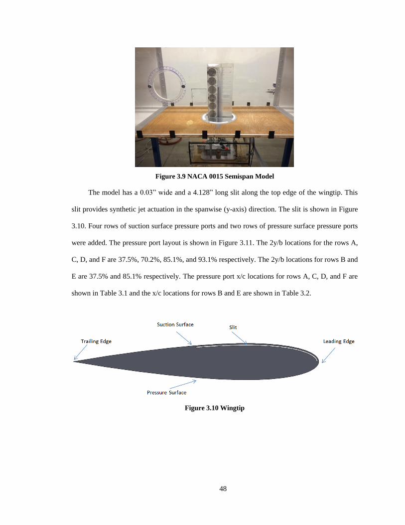
48
Figure 3.9 NACA 0015 Semispan Model
The model has a 0.03” wide and a 4.128” long slit along the top edge of the wingtip. This
slit provides synthetic jet actuation in the spanwise (y-axis) direction. The slit is shown in Figure
3.10. Four rows of suction surface pressure ports and two rows of pressure surface pressure ports
were added. The pressure port layout is shown in Figure 3.11. The 2y/b locations for the rows A,
C, D, and F are 37.5%, 70.2%, 85.1%, and 93.1% respectively. The 2y/b locations for rows B and
E are 37.5% and 85.1% respectively. The pressure port x/c locations for rows A, C, D, and F are
shown in Table 3.1 and the x/c locations for rows B and E are shown in Table 3.2.
Figure 3.10 Wingtip
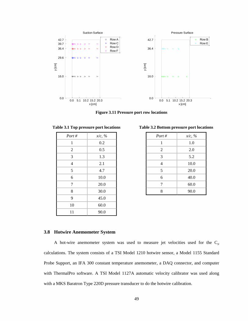
49
Figure 3.11 Pressure port row locations
3.8 Hotwire Anemometer System
A hot-wire anemometer system was used to measure jet velocities used for the Cµ
calculations. The system consists of a TSI Model 1210 hotwire sensor, a Model 1155 Standard
Probe Support, an IFA 300 constant temperature anemometer, a DAQ connector, and computer
with ThermalPro software. A TSI Model 1127A automatic velocity calibrator was used along
with a MKS Baratron Type 220D pressure transducer to do the hotwire calibration.
0.0 5.1 10.2 15.2 20.3 0.0
16.0
29.6
36.4
39.7
42.7
x [cm]
y [cm
]
Suction Surface
Row A
Row C
Row D
Row F
0.0 5.1 10.2 15.2 20.3 0.0
16.0
36.4
42.7
x [cm]
y [cm
]
Pressure Surface
Row B
Row E
Table 3.1 Top pressure port locations
Port # x/c, %
1 0.2
2 0.5
3 1.3
4 2.1
5 4.7
6 10.0
7 20.0
8 30.0
9 45.0
10 60.0
11 90.0
Table 3.2 Bottom pressure port locations
Port # x/c, %
1 1.0
2 2.0
3 5.2
4 10.0
5 20.0
6 40.0
7 60.0
8 90.0
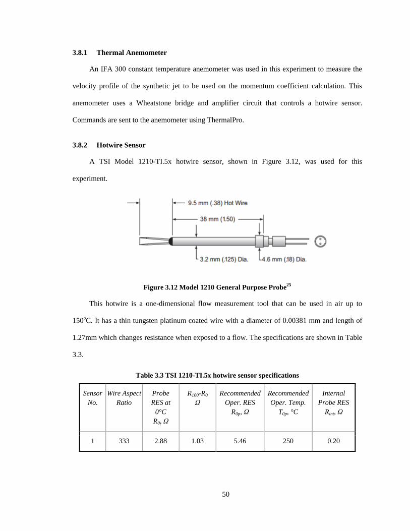
50
3.8.1 Thermal Anemometer
An IFA 300 constant temperature anemometer was used in this experiment to measure the
velocity profile of the synthetic jet to be used on the momentum coefficient calculation. This
anemometer uses a Wheatstone bridge and amplifier circuit that controls a hotwire sensor.
Commands are sent to the anemometer using ThermalPro.
3.8.2 Hotwire Sensor
A TSI Model 1210-TI.5x hotwire sensor, shown in Figure 3.12, was used for this
experiment.
Figure 3.12 Model 1210 General Purpose Probe25
This hotwire is a one-dimensional flow measurement tool that can be used in air up to
150oC. It has a thin tungsten platinum coated wire with a diameter of 0.00381 mm and length of
1.27mm which changes resistance when exposed to a flow. The specifications are shown in Table
3.3.
Table 3.3 TSI 1210-TI.5x hotwire sensor specifications
Sensor
No.
Wire Aspect
Ratio
Probe
RES at
0°C
R0, Ω
R100-R0
Ω
Recommended
Oper. RES
R0p, Ω
Recommended
Oper. Temp.
T0p, °C
Internal
Probe RES
Rint, Ω
1 333 2.88 1.03 5.46 250 0.20

51
The hotwire sensor was attached to a dual sensor TSI Model 1155-6 Standard Probe
Support. This support was used for mounting the hotwire during calibration and during fixturing
for the Cµ test.
3.8.3 Automatic Velocity Calibrator
A TSI Model 1127A automatic velocity calibrator was used to calibrate the hotwire sensor.
A schematic of velocity calibrator system is shown in Figure 3.13. An air supply is connected to a
filter/regulator assembly to condition the air entering the calibrator. The pressure is set to 20-30
psi using this assembly. Once the air enters the calibrator, the flow can be adjusted using a fine
and coarse knob. A hotwire sensor is mounted vertically on the calibrator in front of a 10 mm
opening out of which the velocity is controlled. A MKS Baratron Type 220D-0100A2B pressure
transducer measures the pressure differential of this flow. This differential is sent to the computer
and converted to velocity value with ThermalPro. The thermocouple was not used as the
temperature of the flow stays nearly constant and a correction was not needed.
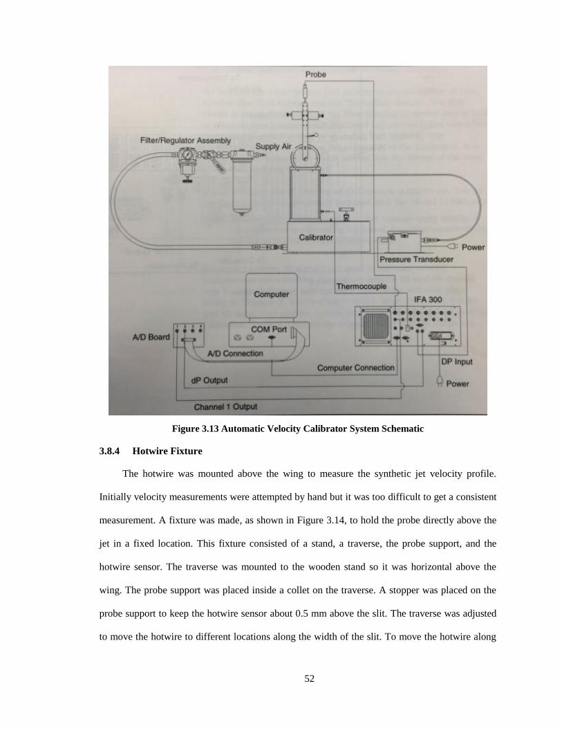
52
Figure 3.13 Automatic Velocity Calibrator System Schematic
3.8.4 Hotwire Fixture
The hotwire was mounted above the wing to measure the synthetic jet velocity profile.
Initially velocity measurements were attempted by hand but it was too difficult to get a consistent
measurement. A fixture was made, as shown in Figure 3.14, to hold the probe directly above the
jet in a fixed location. This fixture consisted of a stand, a traverse, the probe support, and the
hotwire sensor. The traverse was mounted to the wooden stand so it was horizontal above the
wing. The probe support was placed inside a collet on the traverse. A stopper was placed on the
probe support to keep the hotwire sensor about 0.5 mm above the slit. The traverse was adjusted
to move the hotwire to different locations along the width of the slit. To move the hotwire along

53
the length of the slit, the stand was moved. A micrometer was used to measure the exact location
of the hotwire with respect to the slit.
Figure 3.14 Hotwire fixture

54
4 Analysis
4.1 Momentum Coefficient Calculation
The momentum coefficient was calculated to gauge the strength of the synthetic jet. The
equation used to calculate the momentum coefficient is,
4.1
where is the jet density, is the slit area, is the freestream density, and is the
planform area. A hotwire anemometer system was used to measure the synthetic jet velocity
profile which was time averaged to get the RMS velocity profile. A detailed explanation of the
hotwire test can be found in Section 5.2. The RMS velocity was calculated as,
√
4.2
where u is the instantaneous velocity and n is the number of samples. The RMS velocity
contains the rectified expulsion phases of many jet cycles.
4.2 Coefficient of Pressure Calculation
The equation for the pressure coefficient as shown in Equation 4.3 modified to account for
tunnel effects as shown in Equation 4.4
4.3
( ) 4.4
Where is from the pressure ports, is the tunnel calibration correction for the static
pressure, is the tunnel calibration correction for dynamic pressure, and is the correction due
to wake and solid blockage. These correction factors are obtained in the next few sections.

55
4.2.1 Tunnel Calibration
The tunnel total pressure is measured just inside the flow straightener. The tunnel static
pressure is measured after the exit of the nozzle just before the test section. These pressures are
used in the pressure coefficient calculation (dynamic and static pressure is used but total pressure
is used to calculate dynamic pressure) although they are slightly different from the static and total
pressures in the test section. The total and static pressure in the test section would ideally be used
but during the test, the wing model is taking up the place of the test section and a probe cannot be
inserted. A calibration was done to correct this problem. The test section pressures were measured
using a pitot-static tube and a correction was made using
4.5
4.6
4.7
Where K is a correction factor applied to the tunnel pressures and the subscript A denotes
the pressures measured by the pitot-static tube. Kq, Kp, and Kt, were found to be 1.001, 1.012, and
1.025 respectively.
4.2.2 Solid & Wake Blockage
Solid Blockage occurs when walls of the tunnel confine the area that the air stream has to
flow around the wing. This essentially pushes the streamlines towards the wing model surface
increasing the velocity of the air as it flows around the model. The Solid and Wake Blockages
were calculated using the procedures given in Barlow26
. The equation for the solid blockage is
given as
4.8

56
Where K is the body shape factor, τ is a parameter based on figure 10.3 in Barlow26
, V is
the volume of the model, and C is the test section area. The solid blockage in this experiment was
found to be 0.0073 therefore there is only a 0.73% increase in velocity due to the presence of the
wing.
The wake blockage is similar to the solid blockage except it is due to the wake of the
model. In free air conditions, the flow would be able to expand around the wake. Because there
are tunnel walls, the flow cannot expand and must speed up to get past the wake. The correction
for this is
4.9
Where is the uncorrected drag coefficient, is the induced drag coefficient, and
is the zero angle of attack drag coefficient. If is less than zero the whole term
is set to zero. This term is used to account for separated flow and a negative value would mean
that the flow is not separated. The wake blockage is different for each angle of attack. For α =10
degrees at Re = 100,000, the wake blockage is 0.0047.
The solid and wake blockage are used to correct the freestream dynamic pressure by using
4.10
4.11
Where is the correction factor applied to the actual freestream dynamic pressure.
4.2.3 Buoyancy Correction
The tunnel static and dynamic pressure varies across the length of tunnel. This is because
the boundary layer grows in the tunnel walls as the air flows through the tunnel. This thickening
of the boundary layer decreases the effective wind tunnel cross section increasing its speed if the
actual cross section remains fixed. A well designed tunnel will have a minimal increase in speed

57
along its length. This increase in speed increases the drag on the model, hence the need for a
buoyancy correction. The buoyancy corrections were calculated using the procedures given in
Barlow26
. The equation for this correction is,
4.12
Where the body shape factor and t is the wing thickness. Dp/dl was calculated by running
a pitot-static probe along the length of the test section and seeing how the pressure varied. A plot
of this variation is shown in Figure 4.1
Figure 4.1 Wind tunnel lengthwise variation in static pressure, total pressure, and
dynamic pressure
Dp/dl was calculated to be 8.6e-6 psi/ft, which is negligible. The using this value, the
buoyancy corrections comes out to 2.34e-08. This value can be neglected because is a few orders
of magnitude smaller than the error in the drag.
0 2 4-1.020
-1.010
-1.000
P P
itot,
psfg
0 2 4-0.480
-0.460
-0.440
Pt P
itot,
psfg
0 2 40.520
0.540
0.560
q
Pitot,
psfg
Test Section Location, ft

58
4.3 Sectional Force Coefficients
The model contains two complete rows of pressure ports at 2y/b = 37.5% and 85.1%. These
are called “Rows A & B” and “Rows D & E” respectively. A pressure integration was done to
obtain the section lift coefficient at each of these rows. The normal and axial coefficient forces
can be found using a simple panel method. The panels are set up such that each pressure port on
the airfoil is either the start or end of the panel as shown in Figure 4.2 where the points depict the
locations of the pressure ports.
Figure 4.2 Panels used in pressure integrations
Knowing the pressure coefficient, x and y locations of the pressure ports on the airfoil, the
normal and axial forces and be represented as a sum of these pressures along the entire airfoil.
The normal and axial force coefficients are,
∑ (
)
(
) 4.13
∑ (
)
(
) 4.14
where i is the port index, x is the x-location of the pressure port, y is the y-location of the
pressure port, and the pressure coefficients are averaged along the panel. The lift and drag can be
found using the normal and axial forces on the airfoil. The lift and drag coefficient can be written

59
in terms of the normal and axial coefficients and angle of attack. The lift and drag coefficients
are,
4.15
4.16
where cn, ca, and α are normal and axial forces and angle of attack respectively.
4.4 Direct Load Measurement
An Omega LCFD-1KG load cell was used to measure the aerodynamic loads on the wing.
Before this could be done, the load cell had to be calibrated. The calibration was done by hanging
a series of weights from the wing and measuring the output. LabVIEW was used to measure the
output. Each reading consisted of 30,000 samples at a 10,000 Hz sample rate. A plot of the
calibration curve is shown in Figure 4.3.
Figure 4.3 Load cell calibration curve
The weights used were 0, 1/8, 1/4, 1/2, 1, 1.5 lb. The plot is linear with an R-squared value
of 1. The equation of the calibration curve is

60
4.17
Where F is the applied load and V is the voltage. The lift and drag on the wing will be
calculated using this equation. A 1 lb. weight was hung from the bearing plate to pull the plate
into the load cell. This preload was meant to protect the load cell by preventing any small
vibrations from slamming the plate into the load cell. The y-intercept does not read 1lb because
the weight was hung at an angle. The weight was hung this way due to space restrictions inside
the airtight case. The weight was hung exactly the same orientation for each test. To change from
measuring lift to measuring drag , the load cell support structure is rotated 90 degrees. This
calibration was done with the load cell in the lift position. A calibration was also done with the
load cell in the drag position and the results were identical, therefore, this curve could be used for
both load cell orientations.
The lift coefficient and drag coefficients were calculated using
4.18
4.19
Where L is the lift, D is the drag, is the corrected freestream dynamic pressure and S is
the planform area. Note that the planform area is in this equation is based on the half wing
4.5 Uncertainty Analysis
Three major groups of data were taken for this experiment: Hotwire data to calculate the
momentum coefficient, pressure data to view the pressure distribution and the sectional lift
coefficients, and load cell data to measure the lift and drag on the wing directly. Uncertainty
analysis was necessary to ensure the reliability of the data used in this experiment. The
uncertainty can be expressed as

61
√(
)
(
)
(
)
4.20
Where the is the uncertainty or error in the measurement. Detailed derivations,
calculations, and explanations of how the error for each group of data wwas obtained are shown
in Appendix 7B.

62
5 Experimental Procedure
5.1 Hotwire Calibration
In order to get accurate velocity readings from the hotwire, it needed to be calibrated. This
was done using the automatic velocity calibrator. To begin the calibration, the probe was
mounted to the calibrator. The probe can be mounted to the calibrator in several orientations. For
this experiment, it was mounted in the vertical position since that is how it will be used for the
momentum coefficient calculation. Next, the shop air supply was connected and ThermalPro was
started. In ThermalPro, the maximum and minimum velocities expected in the experiment were
defined as 50 m/s and 0 m/s respectively. After this, the cable resistance and probe tare resistance
were measured. ThermalPro was then used to develop a table with velocity points for calibration,
which were clustered near high gradient areas in the calibration curve. The hotwire resistance
would then need to be measured at each of these velocity points. This was done by adjusting the
fine and coarse knobs on the calibrator until the velocity of the calibrator matched the velocity in
the table for each point. The MKS Baratron Type 220D-0100A2B pressure transducer was used
to measure upstream pressure used to back out the calibrator velocity. Figure 5.1 shows the
calibration curve that was obtained though the hotwire calibration. The values in the top right of
the calibration curve show the constants for the 4th order polynomial calibration curve.
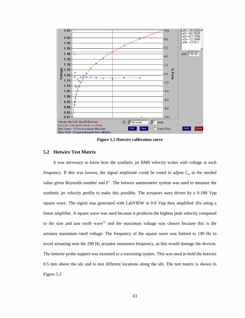
63
Figure 5.1 Hotwire calibration curve
5.2 Hotwire Test Matrix
It was necessary to know how the synthetic jet RMS velocity scales with voltage at each
frequency. If this was known, the signal amplitude could be tuned to adjust Cµ to the needed
value given Reynolds number and F+. The hotwire anemometer system was used to measure the
synthetic jet velocity profile to make this possible. The actuators were driven by a 0-180 Vpp
square wave. The signal was generated with LabVIEW at 0-9 Vpp then amplified 20x using a
linear amplifier. A square wave was used because it produces the highest peak velocity compared
to the sine and saw tooth wave21
and the maximum voltage was chosen because this is the
actuator maximum rated voltage. The frequency of the square wave was limited to 180 Hz to
avoid actuating near the 290 Hz actuator resonance frequency, as this would damage the devices.
The hotwire probe support was mounted to a traversing system. This was used to hold the hotwire
0.5 mm above the slit and to test different locations along the slit. The test matrix is shown in
Figure 5.2

64
Figure 5.2 Hotwire test matrix
Each acquisition consisted of 8,000 samples at a 20,000 Hz sampling frequency. Four
different tests were completed. For the frequency test, the hotwire was placed near the center of
the slit and acquisitions were taken at actuator frequencies every 10 Hz from 10 to 120 Hz at 180
Vpp. For the width test, the hotwire was placed just inside the slit and moved across the 0.04”
width in 5 equally spaced increments taking data at each location. For the length test, data was
acquired in eleven equally-spaced locations along the length of the slit starting at the side nearest
to the leading edge and ending on the side closest to the trailing edge. For this test, the hotwire
was placed at half-width at each location. For the amplitude test, the actuators were excited at 100
Hz and the hotwire was placed at the center of the slit. The voltages tested were 2, 3, 4, 10, 20,
40, 60, 80, 100, 120, 140, 160, and 180 Vpp to see how the RMS velocity profile scales with
amplitude. Using this data, an interpolation could be performed to find Cµ at a given F+ and
Reynolds number.
5.3 Wing and Load Cell Apparatus Preparation
Before the wind tunnel test could begin, the wing model and the load cell apparatus needed
to be prepared. First, the suction surface slits used for separation control were covered with
scotch tape. A smooth layer of wax was applied in to any rough areas on the model covering
features such as screw holes, leading and trailing edges, and the junction between the wingtip and
the wing. The rails were then lubricated with LPS to minimize static friction in the bearings. A
Parameter
Test
Sampling Freq, Hz
Samples 8,000
20,000
Frequency
10:10:120 Hz
Width
5 equally spaced locations
Length
11 equally spaced locations
Amplitude
0-180 Vpp

65
weight was hung off a pulley inside the airtight case to pull the wing into the load cell. This was
done to prevent the wing from slamming into the load cell and damaging it as soon as the tunnel
is turned on. After this, the pressure ports were all checked for leaks by covering the port and
creating a vacuum with a vacuum pump. There was no leak if the vacuum held. After this, the
wind tunnel insert containing the wing was put into the tunnel and any gaps where air could leak
into the tunnel were sealed with scotch tape.
5.4 Calibrating Lift and Drag Directions
It was necessary to align the rails perpendicular to the freestream when measuring lift and
parallel to the freestream when measuring drag. Geometric relations were used between the
tunnel walls, the rotating support, and the wooden insert to make markings that would align the
rails. These tick marks were placed on the rotating support and the wooden insert. When the tick
marks were aligned, the rails were properly oriented. Before each test, the apparatus was checked
to make sure the tick marks were aligned.
5.5 Angle of Attack Calibration
Before the start of the test, the zero lift angle of attack was found. Angle of attack tick
marks were printed on a piece of paper and glued to the rotating support. Because the wing is
symmetric, the zero lift angle of attack is zero. This angle was found by measuring the lift on the
wing using the load cell. The angle of attack was adjusted until one was found that did not result
in any lift. Once this angle was found, a razor blade was inserted between both halves of the
wing. The wing was designed so that the junction of the two halves forms the chord line. The
edge of the razor was used to mark the zero. All following angles used in the test were referenced
from this mark.

66
5.6 Wind Tunnel Test Matrix
The goal of the first test was to get the sectional lift coefficient in two locations along the
span to see how the lift and drag change due to the synthetic jet. The primary independent test
variables were Reynolds number, angle of attack, and excitation amplitude. The dependent
variables of interest were the lift, drag, and the sectional lift coefficients. Each load cell
acquisition consisted of 30,000 samples a sample rate of 10,000 Hz. Each pressure scan consisted
of 400 frames with each frame consisting of 5 averaged data points at a period of 500. The test
matrix is shown in Figure 5.3
Figure 5.3 Wind tunnel test matrix #1
The actuators were run at their maximum rated voltage, which is 180 Vpp. The 4 angles of
attack were chosen to obtain a linear spread for the lift curve. Two Reynolds numbers were
chosen. 105 was chosen because this is what a previous study used. 2x10
5 was chosen to decrease
the error bars in the load cell and pressure data although Cµ was also lowered which meant less
effect on the flow. The idea was to see if increasing Reynolds number could provide better data.
The actuator configuration was either “act off”, “vibration”, or “vib w/ jet”. “Act off” means that
the actuators are not being powered and no actuation exists. “Vibration” means the actuators are
on although scotch tape is being used to cover the slit. When the slit is covered, a relief valve is
opened to relief the cavity pressure. “Vib w/ jet” means that the slit is untaped, the relief valve is
closed, and that a synthetic jet is emitted from the wingtip. The repeatability was checked by
Actuator Config
Reynolds Number
Angle of Attack, deg
Voltage, Vpp 180
[4, 6, 8, 10]
105
Act off Vibration Vib w/ jet
2x10⁵
Act off Vibration Vib w/ jet

67
repeating all of the α = 4 degree Re = 105 points and all of the α = 8 degree Re = 2x10
5 points. F
+
was not kept constant with Reynolds number variation. It was found that F+ did not affect the
flow field around the wing and that Cµ was a much more effective parameter12
. Not holding F+
constant proved benefitial for this test because larger Cµ values could be obtained since the
actuators performed best at 100 Hz and any deviation from 100 Hz (necessary to keep F+
constant) would decrease the Cµ. The F+ calculation is shown in Appendix A
The next test matrix served to assess the effect of momentum coefficient on the flow. Only
pressure data was acquired for this test. The RAD3200 settings were not changed from the
previous test. The test matrix is shown in Figure 5.4
Figure 5.4 Wind tunnel test matrix #2
The angle of attack of 10 degrees and Reynolds number of 105 were chosen because this
was where actuation was believed to have the greatest effect. The “Act off”, “Vibration” and
“Vib w/ jet” cases at 180 Vpp were used as repeats for the previous test. The rest of the cases
were used to see how the effect of actuation scales with Cµ.
5.6.1 Additional Wind Tunnel Test Considerations
Several aspects of this test could lead to erroneous data if not properly addressed. Many of
these were found through trial and error. These aspects are discussed in this section. The model
protruded from the cover plate into the tunnel. An 1/8 inch thick gap exists between the cover
Voltage, Vpp
Actuator Config
Reynolds Number
Angle of Attack, deg 10
100K
Act off Vibration
[0, 40, 80, 120 180]
Vib w/ jet
[0, 40, 80, 120 180]

68
plate and the wing so that the wing does not touch the cover plate and distort the load cell data.
When the angle of attack is changed, the cover plate needs to be rotated as well so that it does not
touch the model and distort data. Also, at Re>200,000 the model starts to deflect slightly. At
these Reynolds numbers, one must look under the tunnel to see if the model is touching the cover
plate when the tunnel is on. The case and cover plate were made clear for these reasons. The next
aspect of this test that could lead to erroneous data is the airtight case. Care must be taken so that
no air leaks into the case. At Re>200,000 one can hear the air entering the case through the gaps
if the case in not sealed properly. The air flows in the tunnel through the 1/8 inch gap between the
cover plate and the model and can significantly affect data.
5.7 Flow Visualization
Oil droplet flow visualization was performed to see if the effect of SJA on the tip shear
stress distribution. Mylar tape was placed over the wingtip on the suction surface, pressure
surface, and tip surface. Droplets of Corning oil with nominal viscosity of 50 cSt were placed on
the tape before the tunnel was turned on as shown in Figure 5.5.
Figure 5.5 Oil droplet distribution used for flow visualization
A green monochromatic light was used to see the droplets more clearly. Due to gravity, the
droplets on the pressure and suction surfaces turned into streaks. This turned out to be fine for the

69
experiment. Once the tunnel is turned on the oil droplets become thinned out showing the
footprint of wing tip vortex on the wing surface as well as the flow direction.
5.8 Stethoscope Boundary Layer Investigation
A stethoscope can be used to evaluate the state of the boundary layer to see if it is turbulent
or laminar. The turbulent boundary layer was distinguished from the laminar boundary layer by
listening to the flow. When the flow was turbulent, pressure fluctuations due to turbulence could
be heard in the boundary layer. This test was done to see if vibration was tripping the flow and to
ensure boundary layer transition was not occurring in different locations for the “act off”,
“vibration” and “vib w/ jet” test conditions. The test was done at Re = 100,000 and Re = 200,000
at α = 10o. Figure 5.6 shows an image taken during the test
Figure 5.6 Stethoscope boundary layer investigation

70
6 Results and Discussion
First, the momentum coefficient results are shown where a hotwire was used to measure the
jet velocities to observe how the synthetic jet behaves and to calculate the momentum coefficient.
After this, the baseline data for the wing is compared to existing data for similar wings. The
quality of the data is also discussed in this section. Next, the results obtained by analyzing the
pressure data are discussed. These results show both the synthetic jet and vibration affect the
pressure distribution on the wing. The sectional lift coefficients were also obtained at two 2y/b
locations. The effect of vibration and the jet on these coefficients are discussed. The momentum
coefficient is also varied and the effect on the coefficients can be seen with varying Cµ. Finally,
the load cell results are shown which demonstrate the effect of vibration and synthetic jet on the
lift and drag of the wing.
Error bars were not included in the plots to avoid clutter. Appendix B shows sample plots
with error bars included.
6.1 Baseline Data Validation
Validation of the data obtained in this study was a difficult task because of the limited
available data. Pressure, lift, and drag data was necessary although most studies focus on much
higher Reynolds numbers and use 2-D wings. A few studies that were found used wings that are
very similar although not exactly the same as the one used in this study. Because exact data could
not be obtained for our specific model, most of this validation serves to show that the data
obtained in this Thesis falls into a range that would be expected for a wing of this type. Figure 6.1
shows the lift curve for a NACA 0015 2D wing compared against 3D data from this experiment.

71
Figure 6.1 Rows A & B baseline sectional lift compared to 2D NACA 0015 airfoil
data 27
Figure 6.1 shows the Rows A & B baseline sectional lift comparison with published data27
.
The A & B location was chosen because it is the most inboard location of pressure acquisition
and most closesly represents the lift of a 2D wing. The values match relatively closely. It was
expected that the lift would be lower than that of the 2D case although this is not the case. This
source of error can come from a few sources. First, the pressure integration uses distinct points
rather than continuous pressure data. This limits the accuracy of the lift calculation. There is also
error in the accuracy of pressure scanner which factors into the calculation of the lift. Finally, the
pressure integration assumes a perfect NACA 0015 wing. Realistically, inaccuracies in the
manufacturing process make this not true. In general though, this plot shows that the section lift is
in the range that would be expected for this wing.
Next, it was necessary to verify the the existence of the laminar separation bubble. Durring
the testing process, spikes in Cp were seen between an x/c 0.15 and 0.5. At first it was thought to
be leaks in the pressure ports or a malfunction in the pressure scanner. After some more testing it

72
was realized that the spike in Cp was a laminar separation bubble. The Cp data in this study is
compared to that of another NACA 0015 study28
in Figure 6.2.
Figure 6.2 Rows A & B baseline Cp distribution at Re = 100,000 compared to NACA
0015 infinite wing28
at Re = 60,000
The wing in the comparison study is 2-D and was tested at a Reynolds number of 60,000.
Although these conditions are not ideal for comparison, this study was chosen due to the limited
amount of data available. It can be seen that laminar separation bubbles occur in both cases. The
higher peak Cp values in the comparison study can be attributed to the fact that the wing used in
that study is infinite. An infinite wing has higher lift compared to that of a finite wing hence the
higher Cp values near the leading edge. Also, the the difference in Reynolds number will change
the location of the separation bubble but the goal of this chart is not to match Cp’s exactly, but to
show that the laminar separation bubble does indeed occur.

73
An attempt at validating pressure data with XFOIL was made although it was found that
XFOIL did not give an accurate pressure distribution for a NACA 0015 for Reynolds numbers
used in this study. According to NACA Report 58627
, at a Reynolds number of 100,000 and an
angle of attack of 10 degrees, the sectional lift coefficient should be around 0.85. XFOIL
predicted a lift coefficient of 1.02. XFOIL also showed much more suction on the top surface of
the wing than the results from this study, with a peak Cp of -3.65. This was expected since the lift
was also overpredicted. Therefore, XFOIL could not be used to validate the Cp data. Next, the
variation in section lift along the y-axis was compared to published results in Figure 6.3
Figure 6.3 Baseline sectional lift compared to NACA 0015 non-tripped finite wing
(Re = 500,000 AR = 4)29
at α=10o
Figure 6.3 shows the baseline sectional lift comparison with a study by Greenblatt and
Washburn29
(2003). They report that the lift on a NACA 0015 wing is highest near the root and
decreases until just before the tip. There is an increase in lift near the tip which is most likely
attributed to the low pressure region caused by the tip vortex. The study slightly underpredicts the
baseline data. This can be attributed to the difference in Reynolds number. Greenblatt and

74
Washburn (1937) shows that there is slight variation in lift with Reynolds number for a NACA
0015.
The lift and drag provided by the load cell needed to be validated. Figure 6.4 shows the
total lift for the baseline case compared to that of a study by Marchman et al30
(1998) .
Figure 6.4 Baseline total lift at Re = 200,000 compared to NACA 0015 non-tripped
finite wing (Re =200,000, AR=4)30
The baseline lift seems to fall in a similar range as that of the study by Marchman et al.
(1998) . The lift slope seems to be slightly off than that form the study . This can be due to a
combination of load cell accuracy and accuracy in the model geometry. This figure shows that the
lift falls in a rang that would be expected of a wing of this type.
Validating the drag data was a difficult task because drag is highly dependent on angle of
attack, Reynolds number, Mach number, surface finish, turbulent or laminar flow, aspect ratio,
and many other factors. Many of these parameters are unique to test the particular model
therefore, it is difficult to find data to validate drag. For this validation, several sources were

75
found, as shown in Figure 6.4, to show that the value of drag falls into a range that is expected for
a wing model of this type.
Figure 6.5 Baseline total drag compared against: 1) NACA 0015 finite wing total and
induced drag at Re =200,000 AR = 3 with transition strips31
. 2) NACA 0015 data
from NACA Report 58627
The first source of drag data is 3D total and induced drag data for a NACA 0015 wing with
an aspect ratio of 3, Reynolds number of 200,000, and a tripped boundary layer31
. The total drag
from the study is higher than the drag obtained for the current study. This can be attributed to the
lower aspect ratio and the transition strips. A lower aspect ratio wing has stronger tip effects
which lead to an increased induced drag coefficient compared to a high aspect ratio wing. The
transition strips create turbulent flow over the wing increasing the profile drag. It is reassuring
that the total drag coefficient for the current model is lower than that of the tripped NACA 0015
but higher than the induced drag coefficient. The second source of drag data is 2D profile drag
from a NACA report at a Reynolds number of 166,000. The profile drag is lower than the drag
obtained in this study which is expected because a 2D wing has no induced drag. This trend once
again shows that the data collected in this study is what would be expected for a wing of this type.

76
6.2 Momentum Coefficient
The first step in calculating the momentum coefficient was to get an idea of how the RMS
velocity varies with frequency and amplitude. The hotwire was placed mid slit and acquisitions
were taken. The frequency of the drive signal used to excite the actuators was increased by 10 hz
for each successive aquisition. A plot of frequency vs RMS velocity is shown in Figure 6.6.
30
Figure 6.6 Synthetic jet RMS velocity for a range of frequencies
Interestingly, actuation at 100 Hz provides the highest RMS velocity. It was expected that
the RMS velocity would be constant across the range of frequencies tested. The explanation for
this occurrence was found by observing the jet instantaneous velocity profiles at each frequency,
as seen in Figure 6.7

77
Figure 6.7 Synthetic jet instantaneous velocity profile
Several things can be observed by studying at the velocity profiles. The velocity profile is
positive due to the rectifying nature of the hotwire. The wire can only sense the magnitude of the
flow and cannot sense if the flow is going toward or away from the wire. Therefore, the wire
cannot tell if the jet is ingesting or expelling fluid and shows the entire velocity profile as
positive. The velocity profile also has distinct pattern. At 100 hz there are large peaks followed
0 0.02 0.04 0.06 0.08 0.10
10
20
30
40
Time [s]
Vel
ocity
[m/s
]
10 Hz
0 0.02 0.04 0.06 0.08 0.10
10
20
30
40
20 Hz
0 0.02 0.04 0.06 0.08 0.10
10
20
30
40
30 Hz
0 0.02 0.04 0.06 0.08 0.10
10
20
30
40
40 Hz
0 0.02 0.04 0.06 0.08 0.10
10
20
30
40
50 Hz
0 0.02 0.04 0.06 0.08 0.10
10
20
30
40
80 Hz
0 0.02 0.04 0.06 0.08 0.10
10
20
30
40
100 Hz
0 0.02 0.04 0.06 0.08 0.10
10
20
30
40
120 Hz

78
by small peaks. The large peaks correspond to the out-stroke and the small peaks correspond to
the in-stroke and have been seen similarly in other studies21
. The ingestion peaks are smaller
because of the ingetion flow patterns sensed by the hotwire. The hotwire is placed a slight
distance above the slit to prevent damage to the hotwire filament. Any small movement can bump
the hotwire into the side wall of the slit and break the wire. The hotwire must be placed a small
distance above the slit to minimize this risk. Because of the non-symmetry, the signal could not
be used to calculate the momentum coefficient. The signal had to be rectified based on the out-
stroke signal, as shown in Figure 6.8, so the RMS velocity and momentum coefficient could be
calculated.
Figure 6.8 Rectifed hotwire signal
The final notable observation to be made from Figure 6.7 is the fluidic interference within
the jet at low frequencies. This can be explained by the fact that the synthetic jet is created by the
displacement of 8 different membranes. A pressure fluctuation is created by each disk and travels
outwards at the speed of sound. Since each disk is a different distance from the exit of the jet, the
time it takes for the pressure fluctuation to reach the jet exit is also different for each disk. This
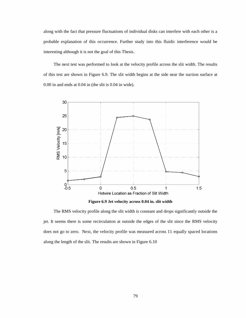
79
along with the fact that pressure fluctuations of individual disks can interfere with each other is a
probable explanation of this occurrence. Further study into this fluidic interference would be
interesting although it is not the goal of this Thesis.
The next test was performed to look at the velocity profile across the slit width. The results
of this test are shown in Figure 6.9. The slit width begins at the side near the suction surface at
0.00 in and ends at 0.04 in (the slit is 0.04 in wide).
Figure 6.9 Jet velocity across 0.04 in. slit width
The RMS velocity profile along the slit width is constant and drops significantly outside the
jet. It seems there is some recirculation at outside the edges of the slit since the RMS velocity
does not go to zero. Next, the velocity profile was measured across 11 equally spaced locations
along the length of the slit. The results are shown in Figure 6.10

80
Figure 6.10 Synthetic jet velocity across slit length
The results show that the RMS velocity is not constant along the slit length. For this
experiment, this is fine because the RMS velocity can be integrated across the slit length to get
Cµ. The results of the amplitude test are shown in Figure 6.11
Figure 6.11 Change in RMS velocity with piezoelectric disk driving signal amplitude

81
These results were as expected. The RMS velocity goes to zero when the voltage is zero and
starts to increase as voltage is increased. The convex nature of the plot shows that the RMS would
reach an asymptote eventually as the voltage is increased although these disks are not rated for
more than 180 Vpp so the voltage was not increased further. With these three plots the
momentum coefficient could be calculated. These tests were done so the momentum coefficient
could be calculated at various frequencies but due to fluidic interference between the 8
piezoelectric disks only frequencies near 100 Hz worked well. Testing was done a 100 Hz
independent of Reynolds number. F+ was allowed to vary because a previous study showed little
change in effect due to F+12
. A plot of Cµ for various Reynolds numbers is shown in Figure 6.12.
Figure 6.12 Momentum coefficient expected at various Reynolds numbers
The results show the momentum coefficient plotted for three Reynolds numbers. Cµ
decreases with Reynolds number and increases with driving signal voltage. Cµ is significantly
higher for Re = 100,000. The results of the plot are tabulated in Table 6.1 for reference in later
sections.

82
Table 6.1 Tabulated Cµ values for f = 100 Hz
Voltage (Vpp)
Momentum Coefficient
Re = 100,000 Re =200,000 Re = 300,000
10 0.01% 0.00% 0.00%
20 0.03% 0.01% 0.00%
40 0.13% 0.03% 0.01%
60 0.24% 0.06% 0.03%
80 0.38% 0.10% 0.04%
100 0.53% 0.13% 0.06%
120 0.69% 0.17% 0.08%
140 0.82% 0.20% 0.09%
160 0.96% 0.24% 0.011%
180 1.10% 0.28% 0.12%
6.3 Pressure Measurement Results
This section discusses the results obtained from the pressure data collected by the RAD
3200 system. The goal of these results was to see how the sectional lift coefficient changes with
actuation. Error bars were omitted from these results to avoid clutter. Appendix B shows the error
analysis and has sample plots with error bars. The sectional lift coefficients for the baseline case
and the actuated case are shown in Figure 6.13.

83
Figure 6.13 Sectional lift coefficient comparison for baseline and actuated cases
The trends in the Re = 100,000 case in Figure 6.13 seemed strange because it was expected
that a jet coming out of the wingtip would have significantly more effect on cl near the wingtip.
It will be later shown why the effect was less significant than expected. These results show that
actuation has a large effect at both 2y/b = 0.38 and 2y/b = 0.85 locations instead of just the most
outboard location at 2y/b = 0.85. During the test, structural vibrations could be felt by touching
the wing. It was predicted that vibration has some effects on these results. The effect of vibration
was isolated from the effect of the synthetic jet by using tape and a relief valve, as discussed in
Section 5.6, to eliminate the synthetic jet while keeping the wing vibrating. The results showing
the effect of vibration are shown in Figure 6.14.

84
Figure 6.14 Sectional lift coefficient comparison isolating the effect of vibration
Figure 6.14 shows that vibration had an effect at Re = 100,000 regardless of the 2y/b
location but it is difficult to see any trends from this data except that vibration had less effect at
Re = 200,000. This could explain the reason the previous plot showed effects for both 2y/b
locations. The effect of the synthetic jet was isolated in Figure 6.15

85
Figure 6.15 Sectional lift coefficient comparison isolating the effect of the synthetic
jet
These results show the expected result from the synthetic jet. The synthetic jet showed
significantly more effect near the wingtip. Rows D & E at 2y/b = 0.85, which are much closer to
the wingtip, show an increase in the sectional lift coefficient with the jet present and Rows A & B
at 2y/b = 0.38 do not. At Re = 200,000 there is less effect which can be attributed to the lowered
momentum coefficient, although the lift is still slightly increased towards the tip.
The cause of the sectional lift coefficient trends was investigated by looking into the Cp
distributions. For the following results, there were no noticeable differences in the pressure
distribution on the pressure surface of the wing due to actuation. Because of this, the Cp
distribution on the pressure surface was omitted to draw more attention to the suction surface.
Appendix B.1. shows a sample plot with the Cp distribution on the pressure surface for reference.
The effect of vibration on the Cp can be seen by looking at Figure 6.16 through Figure 6.19 .

86
Figure 6.16 Row F suction surface Cp distribution at 2y/b = 0.93 showing effect of
wing vibration at F+ = 2.78, Cµ = 0.00, and Re = 100,000
Figure 6.17 Row D suction surface Cp distribution at 2y/b = 0.85 showing effect of
wing vibrationat at F+ = 2.78, Cμ = 0.00, and Re = 100,000
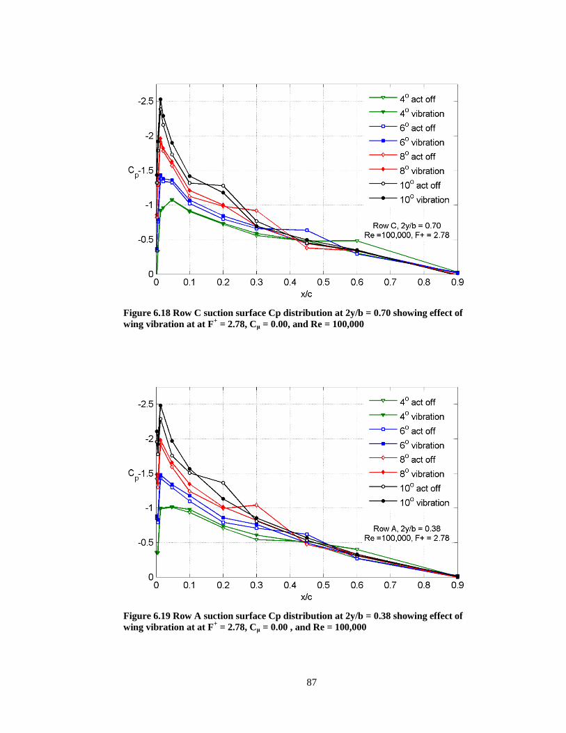
87
Figure 6.18 Row C suction surface Cp distribution at 2y/b = 0.70 showing effect of
wing vibration at at F+ = 2.78, Cμ = 0.00, and Re = 100,000
Figure 6.19 Row A suction surface Cp distribution at 2y/b = 0.38 showing effect of
wing vibration at at F+ = 2.78, Cμ = 0.00 , and Re = 100,000

88
Pressure irregularities indicative of laminar separation bubbles can be seen in Figure 6.16-
Figure 6.19. The laminar separation bubbles become more significant near the root. This is a
well-observed phenomenon for low Reynolds number flows28
. Vibration eliminates this
separation bubble and increases the Cp distribution near the leading edge. At higher Reynolds
number this bubble is much less prevalent. Figure 6.20 shows the Cp distribution for Row A at
2y/b = 0.38 at Re = 200,000. There is no effect near the leading edge although vibration does
have some effect after x/c = 0.3. What can be concluded from these charts is that vibration
eliminates the laminar separation bubble.
Figure 6.20 Row A suction surface Cp distribution at 2y/b = 0.38 showing effect of
wing vibration at at F+ = 1.39, Cμ = 0.00,and Re = 200,000
Next the effect of the synthetic jet was isolated. Figure 6.21 through Figure 6.24 show the
effect of the synthetic jet.
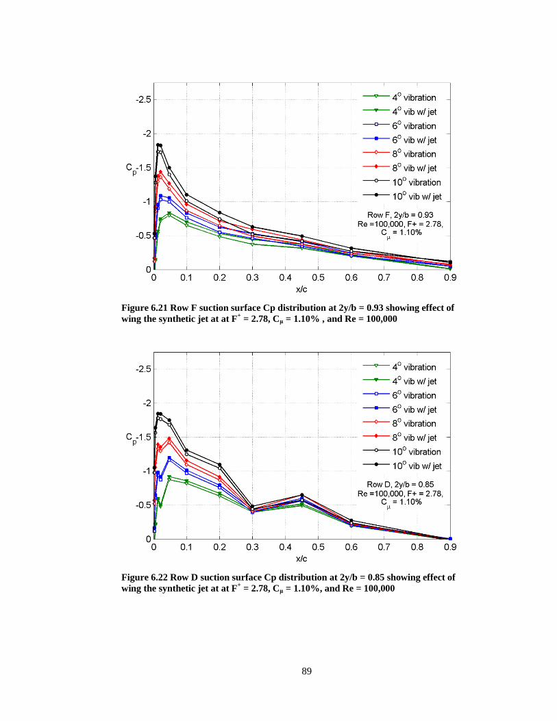
89
Figure 6.21 Row F suction surface Cp distribution at 2y/b = 0.93 showing effect of
wing the synthetic jet at at F+ = 2.78, Cμ = 1.10% , and Re = 100,000
Figure 6.22 Row D suction surface Cp distribution at 2y/b = 0.85 showing effect of
wing the synthetic jet at at F+ = 2.78, Cμ = 1.10%, and Re = 100,000

90
Figure 6.23 Row C suction surface Cp distribution at 2y/b = 0.70 showing effect of
wing the synthetic jet at at F+ = 2.78, Cμ = 1.10% , and Re = 100,000
Figure 6.24 Row A suction surface Cp distribution at 2y/b = 0.38 showing effect of
wing thesynthetic jet at at F+ = 2.78, Cμ = 1.10% , and Re = 100,000
These results were expected from the synthetic jet. The jet increases the suction near the
leading edge to about mid-chord. The effect becomes more significant at 2y/b = 0.70, 0.85 and

91
0.93 closer to the tip since this is where the jet is located. The effect is also larger for higher
angles of attack. This matches what was seen in the sectional lift coefficient results since cl
increased more for higher angles of attack. Figure 6.25 shows the results for Re = 200,000.
Figure 6.25 Row F suction surface Cp distribution at 2y/b = 0.93 showing effect of
wing the synthetic jet at at F+ = 1.39, Cμ = 0.28%, and Re = 200,000
There is much less effect due to the synthetic jet at F+= 1.39. This can be attributed to the
drop in Cµ. An addition test was done to see how the lift coefficient varies with Cµ. The results
are shown in Figure 6.26

92
Figure 6.26 Sectional lift coefficient variation with driving signal amplitude
Figure 6.26 shows several interesting trends. In Figure 6.26 (a) the “vibration” case shows
an initial drop in cl from 0-40 Vpp, then almost no effect from 40-180 Vpp. This deserves some
explanation. An increase in voltage increases the center displacement of the piezoelectric disks
for each actuation cycle and causes more air to be pushed in and out of the slit . A result of this
increased center displacement is an increase in vibration. A direct relationship between voltage
and vibration was observed during the test by phycially feeling the wing vibrate. This suggests
that only a slight amount of vibration (the amount caused by 40 Vpp) is needed to get the
majority of the vibrational effects. After 40 Vpp there is little effect from further increases in
volatage, and thereby increases in vibration. The “vib w/ jet” case in Figure 6.26 (a) shows the
combined effects of the jet and of vibration. The effect of vibration can be seen in the initial drop
in cl from 0-40 Vpp. After this initial drop it can be assumed that vibration does nothing to further
decrease cl. The increase in cl after 40 Vpp is therefore caused by the synthetic jet. There is also
continued increase in cl with increasing Cµ as the voltage increases.

93
Figure 6.26 (b) shows a similar trend where vibration only has impact from 0-40 Vpp. Two
interesting things can be observed from this plot. First, is that there is no increase in cl with
increasing Cµ. This could be because the 2y/b location where the measurements were taken is
farther from the jet exit which is at 2y/b = 1. Another interesting observation is that vibration
caused an increase in cl from 0-40 Vpp instead of a decrease as was seen in Figure 6.26 (a). It is
unkown why vibration causes an increase in one location and a decrease in another. One possible
explanation is that the laminar separation bubble is larger near the 2y/b =0.38 than it is at 2y/b
=0.85, as seen in Figure 6.16 and Figure 6.19, and vibration tends to eliminate this separation
bubble. Therefore, since bubble attachment should increase lift, more of an increase in lift should
be seen near 2y/b = 0.38 where the laminar bubble is more prevelant. Although this would
explain the increase in lift at 2y/b = 0.38 from 0-40 Vpp, the decrease in lift for 2y/b would
require further investigation.
6.4 Load Cell Results
Because the pressure results showed vibrational effects, the load cell data was also acquired
in such a way as to isolate the effect of vibration and the effect of the synthetic jet. The
unactuated and actuated cases are shown in Figure 6.27.

94
Figure 6.27 NACA 0015 lift curve for actuated and unactuated cases
From this plot, it can be seen that actuation slightly increases the lift in Figure 6.27 (a) and
has almost no effect in Figure 6.27 (b). It is unclear if vibration or the jet is causing these results.
Figure 6.28 shows the isolated effect of vibration
Figure 6.28 NACA 0015 lift curve showing the isolated effect of vibration

95
Vibration increases the lift slightly at a Reynolds number of 100,000 although the effect is
very small.. Figure 6.29 shows the effect of the synthetic jet.
Figure 6.29 NACA 0015 lift curve showing the isolated effect of the synthetic jet
A slight increase in lift can be seen due to the synthetic jet at Figure 6.29 (a) while Figure
6.29 (b) shows no effect due to the jet. From these plots it can be concluded that actuation
slightly increases the total lift on the model at the lower Reynolds number but has little to no
effect at higher Reynolds numbers. Although, this is most likely due to the lower Cμ at Re =
200,000. The drag for the unactuated and actuated cases is shown in Figure 6.30.
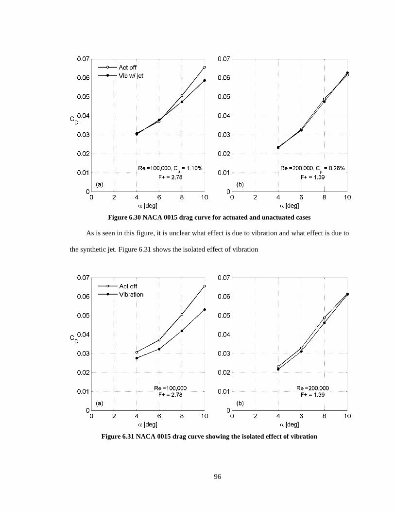
96
Figure 6.30 NACA 0015 drag curve for actuated and unactuated cases
As is seen in this figure, it is unclear what effect is due to vibration and what effect is due to
the synthetic jet. Figure 6.31 shows the isolated effect of vibration
Figure 6.31 NACA 0015 drag curve showing the isolated effect of vibration
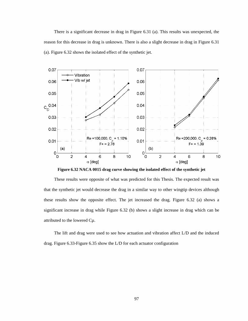
97
There is a significant decrease in drag in Figure 6.31 (a). This results was unexpected, the
reason for this decrease in drag is unknown. There is also a slight decrease in drag in Figure 6.31
(a). Figure 6.32 shows the isolated effect of the synthetic jet.
Figure 6.32 NACA 0015 drag curve showing the isolated effect of the synthetic jet
These results were opposite of what was predicted for this Thesis. The expected result was
that the synthetic jet would decrease the drag in a similar way to other wingtip devices although
these results show the opposite effect. The jet increased the drag. Figure 6.32 (a) shows a
significant increase in drag while Figure 6.32 (b) shows a slight increase in drag which can be
attributed to the lowered Cµ.
The lift and drag were used to see how actuation and vibration affect L/D and the induced
drag. Figure 6.33-Figure 6.35 show the L/D for each actuator configuration

98
Figure 6.33 NACA 0015 L/D curve for actuated and unactuated cases
Figure 6.34 NACA 0015 L/D showing the isolated effect of vibration

99
Figure 6.35 NACA 0015 L/D curve showing the isolated effect of the synthetic jet
Figure 6.33 shows that the cumulative effect of vibration and the jet does not produce any
significant results. Figure 6.34-Figure 6.35 show that vibration increases L/D while the synthetic
jet decreases L/D. The induced drag curves are shown in Figure 6.36 through Figure 6.38.
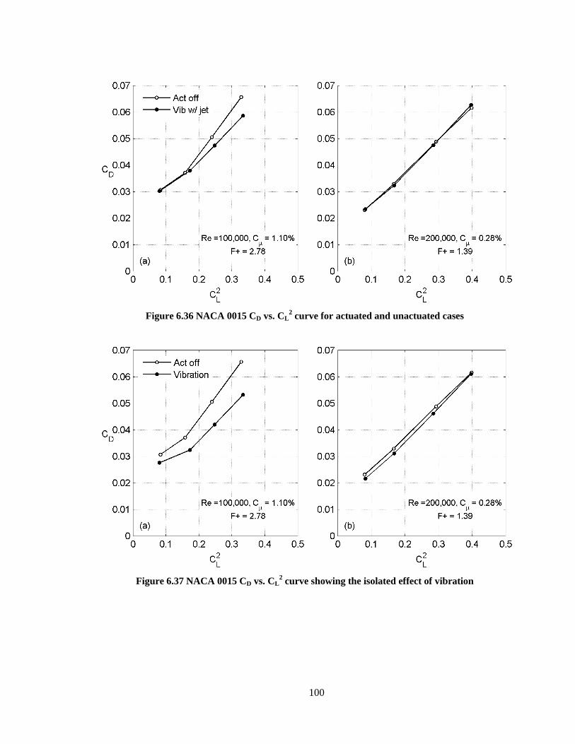
100
Figure 6.36 NACA 0015 CD vs. CL2 curve for actuated and unactuated cases
Figure 6.37 NACA 0015 CD vs. CL2 curve showing the isolated effect of vibration

101
Figure 6.38 NACA 0015 CD vs. CL2 curve showing the isolated effect of the synthetic
jet
Little can be concluded from Figure 6.36 since it contains both the effect of vibration and
the effect of the synthetic jet. Figure 6.37 (a) possibly shows a significant finding. If the linear
portions of the curves in Figure 6.37 (a) are extended, they both interact at about CD = 0.01 at CL
= 0. The slope of the vibration curve has a slightly decreased slope. This means that vibration
should reduce the induced drag by up to as 11.3% at α = 4° to 23.4% at α = 10°. This decrease in
drag was also seen in Figure 6.31. Interestingly, Figure 6.16 did not show any change in the Cp
distribution near the wingtip due to vibration which does not support a reduction in induced drag.
Error analysis was done in Appendix B to see if the results in Figure 6.37 were significant. As
seen in Figure 7.4, the errorbars show that the error in the drag measurement at Re = 105 is too
high to make any definite conclusions about the induced drag reduction using the load cell data.
The synthetic jet results in Figure 6.38 show that there is no change in slope although CD0 is
increased due to the synthetic jet for both Reynolds numbers. This means that the synthetic jet
actually increases the total drag rather than decreases the induced drag as was predicted at the
start of this Thesis.

102
6.5 Oil Film Interferometry Results
The oil film results for the suction surface are shown in Figure 6.39.
Figure 6.39 Oil film interferometry on suction surface (Re = 100,000 α = 10o).
The images on the left show the suction surface without actuation. The top picture starts
with the leading edge and moves down towards the trailing edge. The pictures on the right shows
the same thing except with actuation at Cµ = 1.10% , and F+ = 2.78. The footprint of the tip
vortex can be seen in the unactuated case. This vortex starts at about x/c = 0.3 and moves
downstream and inboard further down the wing. This footprint is caused by the low pressure
region created by the vortex. When the actuators were turned on, the footprint of the vortex was
eliminated. This suggests a that the vortex was pushed off the wingtip or the vortex became so
diffuse that it could not produce low enough pressure to cause the droplets to come together and
form the footprint. Both of these conjectures would reduce the downwash and hence the induced
drag should be reduced. This is consistent with Figure 6.36 which showed a decrease in induced
drag when actuation was triggered. This is a significant result as both flow visualization and
direct drag measurements support a decrease in induced drag. Figure 6.40 shows the pattern on
the tip surface.

103
(a)
(b)
Figure 6.40 Oil film interferometry on tip surface (Re = 100,000 α = 10o). (a)
Actuators off. (b) Actuators on slit uncovered
Actuation seemed to have little effect on the tip surface. There is a secondary vortex
forming from the pressure surface to the tip surface. This vortex was not affected by actuation,
only the primary vortex on the suction surface was affected.
6.6 Stethoscope Boundary Layer Investigation Results
The pressure surface of the model was laminar for both Re = 100,000 and Re = 200,000
independent of whether the model was acutated. The suction surfaces transitioned from laminar
to turbulent in different locations depending on the Reynolds number. Actuation seemed to have
very little effect on the transition point. The transition locations are shown in Table 6.2.
Table 6.2 Laminar to turbulent transition locations α = 10o
Re = 100,000 Re = 200,000
Act off Vibration Vib w/ jet Act off Vibration Vib w/ jet
Rows A &
B
25% 25% 25% 12% 16% 16%

104
It can be seen that the transition point moved upstream as the Reynolds number was
increased but stayed relatively consistent with actuator configuration. These results show that the
effects of the different actuator configurations are not due to a change in transition location.
Rows D &
E
30% 25% 25% 14% 16% 16%
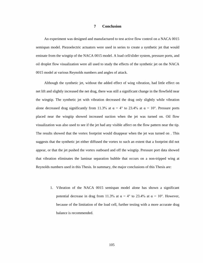
105
7 Conclusion
An experiment was designed and manufactured to test active flow control on a NACA 0015
semispan model. Piezoelectric actuators were used in series to create a synthetic jet that would
eminate from the wingtip of the NACA 0015 model. A load cell/slider system, pressure ports, and
oil droplet flow visualization were all used to study the effects of the synthetic jet on the NACA
0015 model at various Reynolds numbers and angles of attack.
Although the synthetic jet, without the added effect of wing vibration, had little effect on
net lift and slightly increased the net drag, there was still a significant change in the flowfield near
the wingtip. The synthetic jet with vibration decreased the drag only slightly while vibration
alone decreased drag significantly from 11.3% at α = 4° to 23.4% at α = 10°. Pressure ports
placed near the wingtip showed increased suction when the jet was turned on. Oil flow
visualization was also used to see if the jet had any visible affect on the flow pattern near the tip.
The results showed that the vortex footprint would disappear when the jet was turned on . This
suggests that the synthetic jet either diffused the vortex to such an extent that a footprint did not
appear, or that the jet pushed the vortex outboard and off the wingtip. Pressure port data showed
that vibration eliminates the laminar separation bubble that occurs on a non-tripped wing at
Reynolds numbers used in this Thesis. In summary, the major conclusions of this Thesis are:
1. Vibration of the NACA 0015 semispan model alone has shown a significant
potential decrease in drag from 11.3% at α = 4° to 23.4% at α = 10°. However,
because of the limitation of the load cell, further testing with a more accurate drag
balance is recommended.

106
2. The synthetic jet has a significant effect on the flow field near the wingtip. There
was a signifant increase in -Cp at 2y/b = 0.85 and surface oil flow visualization
showed absence of the wingtip vortex footprint with actuation.
3. Pressure port data showed that the laminar separation bubble is eliminated due to
wing vibration
4. The synthetic jet without vibration is not effective at reducing induced drag in the
configuration used in this thesis, showing an increase in drag rather than a decrease.

107
Bibliography
1 Thomas, A. S., “Aircraft Drag Reduction Technology–A Summary”. Advisory Group for
Aerospace Research and Development (AGARD), Report 723, Belgium, 1985.
2 Zimmer, H., “Aerodynamic Optimization of Wings at Subsonic Speeds and the Influence of
Wingtip Design”, NASA TM-88534, 1983
3 Kroo, I. “Nonplanar Wing Concepts for Increased Aircraft Efficiency”. VKI Lecture Series on
Innovative Configurations and Advanced Concepts for Future Civil Aircraft, Stanford,
2005.
4 Rossow, V. J., and James, K. D., “Overview of Wake-Vortex Hazards During Cruise,” Journal
of Aircraft, Vol. 37, No. 6, 2000, pp. 960–975. doi:10.2514/2.2723
5 Filippone, A., “Analysis of Carbon-Dioxide Emissions from Transport Aircraft,” Journal
Aircraft, Vol. 45, No. 1, Jan.–Feb. 2008, pp. 185–197. doi:10.2514/1.31422
6 Whitcomb, R. T., “A Design Approach and Selected Wind-Tunnel Results at High Subsonic
Speeds for Wing-Tip Mounted Winglets”, NASA-TN-D-8260, 1976
7 KROO, I. “Drag due to lift: Concepts for prediction and reduction”, Annual Rev: Fluid
Mechanics, 2001, 33, pp 587-617.
8 McLean D., "Wingtip Devices: What they Do and How They Do it," presented at the Boeing
Performance and Flight Operations Engineering Conference 2005.
9 Mineck, R.E., “Study of potential aerodynamic benefits from spanwise blowing at wingtip”,
NASA technical report 3515, 1995.
10 Seifert A., Darabi A., and Wygnanski, I., “Delay of Airfoil Stall by Periodic Excitation”,
Journal of Aircraft, Vol. 33, No. 4, 1996, 691–698.

108
11
Smith, B.L. and Swift, G.W., ‘‘A comparison between synthetic jets and continuous jets,’’
Experiments in Fluids, Vol. 34, pp. 467–472, 2003.
12 Margaris, P., and Gursul, I., “Wing Tip Vortex Control Using Synthetic Jets,” The Aeronautical
Journal, Vol. 110, No. 1112, 2006, pp. 673–681.
13 Boesch, G., Vo, H., Savard, B., Wanko-Tchatchouang, C., and Mureithi, N., “Flight control
using wing-tip plasma actuation," Journal of Aircraft, Vol. 47, No. 6, 2010, pp. 1836-1846.
14 Chappell S., Angland D., “Active Control of a Wing Tip Vortex with a Dielectric Barrier
Discharge Plasma Actuator” AIAA Paper 2012-2952, 6th AIAA Flow Control Conference,
New Orleans, Louisiana, 25-28 June 2012, 10.2514/6.2012-2952
15 S.I. Green, “Fluid Vortices” in: Fluid Mechanics and Its Applications, Kluwer Academic
Publisher, 1995, pp. 427–470.
16 Giuni, M., and Green, R.B. “Vortex formation on squared and rounded tip,” Aerospace Science
and Technology, 29 (1). pp. 191-199
17 S. Gao, J.Z. Zhang, X.M. Tan “Experimental study on heat transfer characteristics of synthetic
jet driven by piston actuator” Sci. Chin. Tech. Sci., 55 (2012), pp. 1732–1738
18 Crittenden, T. and Glezer, A., “A High-Speed Compressible Synthetic Jet,” Physics of Fluids,
Vol. 18, No. 1, 017107, 2006
19 J. S. Agashe, M. Sheplak, D. P. Arnold, and L. N. Cattafesta, "MEMS-based Actuators for
Flow-Control Applications," in IUTAM Symposium on Flow Control and MEMS, J. F.
Morrison, Ed.: Springer, September 2006, pp. 25-32.
20 Lopez, O. and Moser, R., “Computational Study of a NACA4415 airfoil using synthetic jet
control”, Ph.D. thesis, The University of Texas at Austin, 2009

109
21
Mane, P., Mossi, K., and Bryant R., “Synthetic Jets with Piezoelectric Diaphragms”.
Proceedings of SPIE Vol. 5761.
22 P. Mane, “Experimental Design and Analysis of Piezoelectric Synthetic Jets in Quiescent Air”,
Masters Thesis, Virginia Commonwealth University, Fall 2005.
23 Piezo Systems, INC. http://www.piezo.com/prodbm5disk.html (accessed July 2, 2013)
24 Omega Engineering. http://www.omega.com/Pressure/pdf/LCFD.pdf (accessed December
2013)
25http://www.tsi.com/uploadedFiles/_Site_Root/Products/Literature/Catalogs/Hotwire_Catalog_2
980465.pdf
26 Barlow, J. B. Rae, W. H. Pope, A., Low Speed Wind Tunnel Testing, Third Edition, John
Wiley and Sons, Inc., (1999)
27 Jacobs, Eastman N Sherman, Albert. “Airfoil section characteristics as affected by variations of
the Reynolds number”. NACA Report 586, (1937).
28 Leon L., “Experimental Testing of Low Reynolds Number Airfoils for Unmanned Aerial
Vehicles”, Masters Thesis, Institute for Aerospace Studies University of Toronto, 2013
29 D. Greenblatt, and A. E. Washburn, “Influence of Finite Span and Sweep on Active Flow
Control Efficacy”. AIAA Journal 46:7, 1675-1694, 2003
30 J.F. Marchman, C.L Gunther and J.F Gundlach, “Semi Span Testing at Low Reynolds
number”, AIAA 36th Aerospace Science Meeting and Exhibits, January 12-15, 1998, Reno,
NV.
31 Lee, T., Birch, D., Mokhtarian, F., and Kafayeke, F., “Structure and Induced Drag of a Tip
Vortex,” Journal of Aircraft, Vol. 41, No. 5, 2004, pp. 1138–1145. doi:10.2514/1.2707

110
Appendices
A Sample Calculations
Reynolds number (temperature of 64oF)
Dynamic pressure correction
Static pressure correction
Total pressure correction
Pressure coefficient (Re = 100,000 α = 10 Row C x/c = 2.1%)
( )
Wing planform area

111
Wing volume
(
) (
)
Solid blockage correction (multiplied by ½ because the model is half of a wing)
(
)
(
)
Wake blockage correction (Re = 100,000 α = 10. Assuming no separation)
(
)
Dynamic pressure correction due to solid and wake blockage
Lift ( Re = 100,000 , α = 10)
Lift Coefficient ( Re = 100,000 , α = 10)
Drag ( Re = 100,000 , α = 10)

112
Drag Coefficient ( Re = 100,000 , α = 10)
Non-dimensional Fequency, F+ ( Re = 100,000, f = 100 Hz )

113
B Uncertainty Analysis
B.1 Pressure Coefficient
The pressure scanner used to acquire pressure data for the Cp calculation used two sets of
pressure transducers. Ports 1-32 used pressure transducers with a range of +- 2.491 KPa (10
inH2O) and ports 33-64 used transducers with a range of +- 249.1 Pa (1 psid). Rows B, C, E, and
the first 4 ports of row A (starting at the leading edge) used transducers 1-32. Rows D, F, the
tunnel static pressure, and the tunnel total pressure used ports 33-64. The error in the pressure
values consisted of random and systematic error, which were both included in the error
calculation. The random error was found by taking the standard deviation of five consecutive
scans consisting of 400 frames each with the tunnel off. The systematic error consists of the drift
and zero offset after CALZ is commanded to the system. The zero offset error was eliminated by
taking a reading with the tunnel off after calibration and using the non-zero pressure readings as
tares. The drift was found by measuring how much the “tunnel off” pressure values drifted at the
end of the test session. The following sample error calculation is for the Row C port at x/c = 2.1%
at α=10 and Re = 100,000.

114
( )
( )
( )
( )
√(
)
(
)
(
)
√( ( ))
( ( ))
( ( ))
The error bars for Rows A & B can be seen in the following figure.
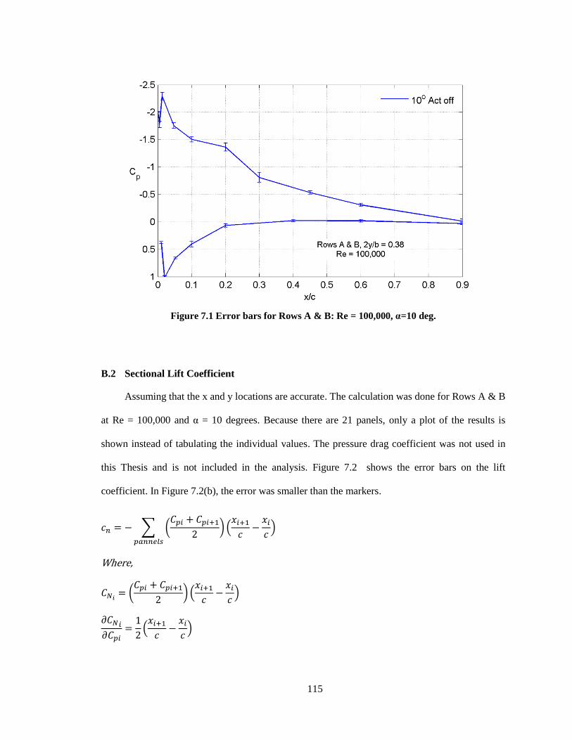
115
Figure 7.1 Error bars for Rows A & B: Re = 100,000, α=10 deg.
B.2 Sectional Lift Coefficient
Assuming that the x and y locations are accurate. The calculation was done for Rows A & B
at Re = 100,000 and α = 10 degrees. Because there are 21 panels, only a plot of the results is
shown instead of tabulating the individual values. The pressure drag coefficient was not used in
this Thesis and is not included in the analysis. Figure 7.2 shows the error bars on the lift
coefficient. In Figure 7.2(b), the error was smaller than the markers.
∑ (
)
(
)
Where,
(
) (
)
(
)
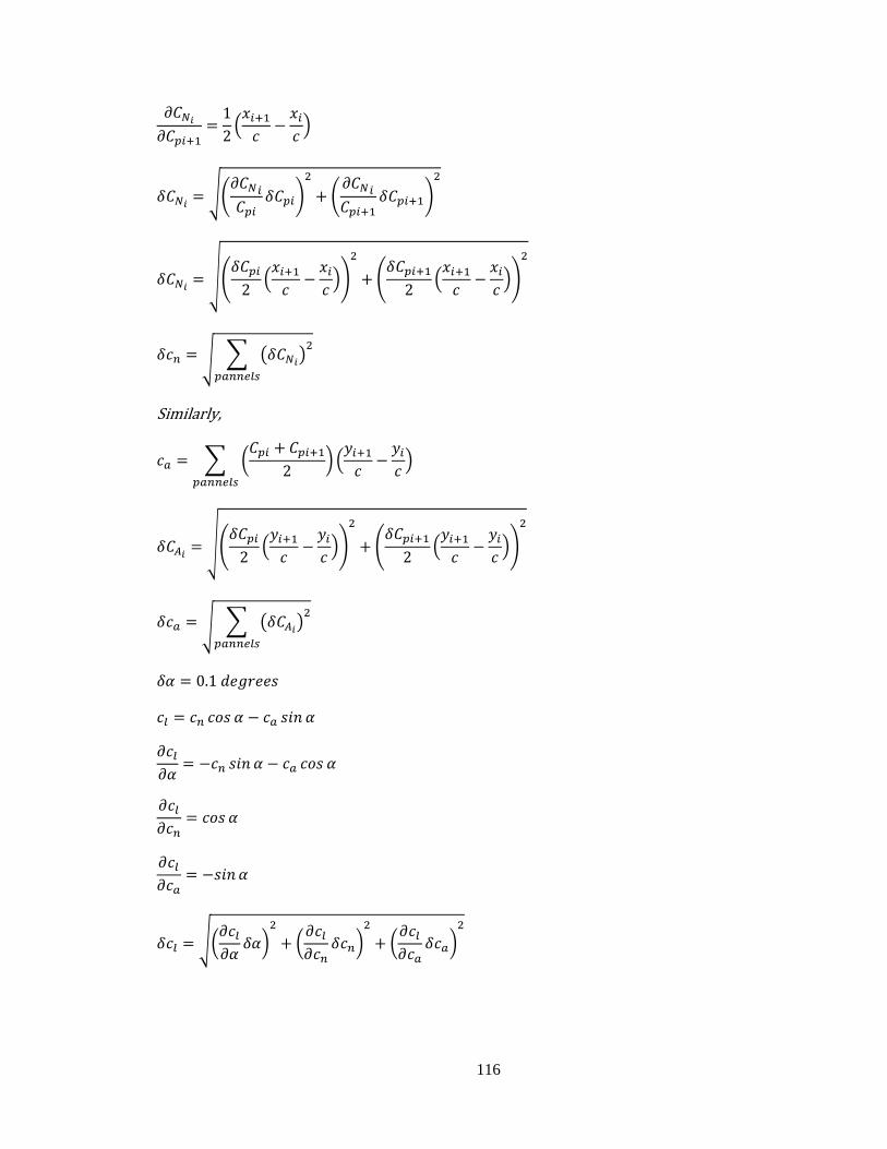
116
(
)
√(
)
(
)
√(
(
))
(
(
))
√ ∑ ( )
Similarly,
∑ (
)
(
)
√(
(
))
(
(
))
√ ∑ ( )
√(
)
(
)
(
)

117
Figure 7.2 Lift coefficient error bars
B.3 Lift and Drag Coefficient Error
The accuracy of the load cell is 0.15% FSO. For this load cell, the FSO is 1kg (2.2 lb) so the
accuracy is 0.0015 kg (0.0033 lb). Assuming the freestream dynamic pressure and planform area
are accurate, the error in the lift coefficient is
Where,
For the drag coefficient the error is
Where,
The following sample calculation shows f r Re a d α
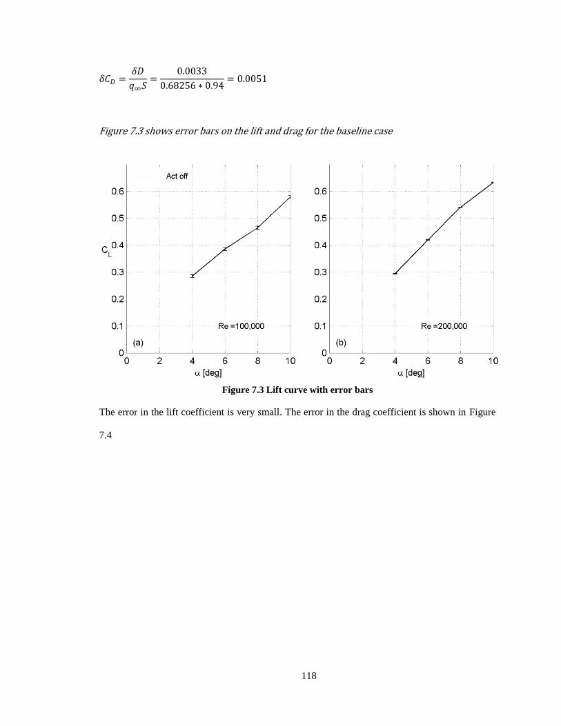
118
Figure 7.3 shows error bars on the lift and drag for the baseline case
Figure 7.3 Lift curve with error bars
The error in the lift coefficient is very small. The error in the drag coefficient is shown in Figure
7.4

119
Figure 7.4 Drag curve with error bars
The error in the drag coefficient at Re = 100,000 is very large. This is because the
magnitude of the drag was very low so the 0.0015 kg (0.0033 lb) error in the load cell had a large
impact. The following sample calculation shows for Re = 100,000 and α = 4.
At Re =200,000 the error was much lower because the drag increased significantly. It is
possible that the error was smaller than what is shown in Figure 7.4. The accuracy of the load cell
used in the error analysis was the worst case error as specified by the manufacturer. Durring
testing, for each angle of attack there were several repeated points taken to verify the repeatability
of the data. A sample error plot for the R=100,000 baseline drag using the standard deviation
between the repeat values is shown in Figure 7.5. The error bars are much smaller than they were
in Figure 7.4. This shows that it is quite possible that there was less error than what was specified
as the worst case by the manufacturer.

120
Figure 7.5 Drag curve with error bars showing error calculate using the standard
deviation of repeat load cell readings
B.4 Momentum Coefficient Error
The error in the momentum coefficient comes from a few sources. The first is human error
in the positioning of the hotwire since the hotwire was placed in several locations which were
measured with a caliper and micrometer depending on the application. Another source of error
comes from the fact that the hotwire could not be placed at the optimal location just inside the jet.
This could not be done because if the hotwire is positioned too close it could easily bump into the
slit and break. Another source of error is the accuracy of the anemometer itself. The error at each
calibration point was recorded by the anemometer. The anemometer error can be using
Where is the instantaneous jet velocity, V is the voltage, and A-D are the 4th order
polynomial constants. Looking at Figure 5.1, the error in the voltage is about 1 percent. The
error can be calculated as follows.
Where,

121
Therefore,
√[ ]
Where
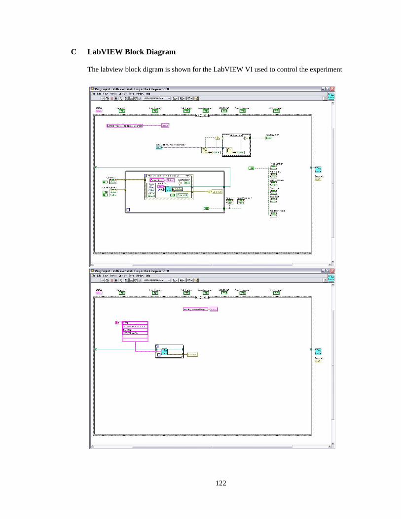
122
C LabVIEW Block Diagram
The labview block digram is shown for the LabVIEW VI used to control the experiment

123

124