Experimental and numerical study of the turbulence

characteristics of air flow around a research vessel

Stephane Popinet∗ Murray Smith†

Craig Stevens‡

National Institute of Water and Atmospheric Research,PO Box 14-901 Kilbirnie, Wellington, New Zealand

Submitted to Journal of Atmospheric and Oceanic Technology

October 1, 2003

Abstract

Airflow distortion by research vessels has been shown to significantly affect micro-meteorological

measurements. This study uses an efficient time-dependent Large Eddy Simulation numerical tech-

nique to investigate the effect of the research vessel Tangaroa on both the mean and turbulent

characteristics of airflow. Detailed comparison is given between the numerical results and an exten-

sive experimental dataset. The study is performed for the whole range of relative wind directions

and for instruments located in regions of high and low flow distortion. The experimental data show

that both the normalised wind speed and normalised standard deviation are only weakly dependent

on wind speed, ship speed, ship motion and sea state, but strongly dependent on relative wind

direction. Very good agreement is obtained between the experimental and numerical data for the

mean flow, standard deviation and turbulence spectra, even in areas of strong turbulence.

1. Introduction

Interactions between the atmosphere and ocean form an important part of the climate system. Mea-surement of fluxes of momentum, heat, gases, and the accurate parameterisation of those fluxes, arerequired for global climate and weather models. Research vessels are the most common measur-ing platform for these flux measurements but they are also susceptible to airflow distortion effectsaround the hull and superstructure. It is therefore important to understand and accurately model theinfluence of the sampling platform on airflow and turbulence.

Yelland et al. (1998) examined two airflow effects: a) the acceleration/deceleration of flow and b)the tilt of the flow that results in air with turbulent characteristics from a different height being mea-sured. These effects influence the drag coefficient for neutral atmospheric stability (CD10N

) calculatedusing the inertial dissipation method. This method is preferred at sea since it uses frequencies in theinertial subrange of turbulence that are well above the frequencies associated with the wave-inducedplatform motion. The drag coefficient is given by:

CD10N=

(kzε)2/3

U210N

,

∗s.popinet@niwa.co.nz†m.smith@niwa.co.nz‡c.stevens@niwa.co.nz

1

where k is the von Karman constant, z is the height at which the air originated, ε is the turbulentdissipation rate (determined from spectra of wind fluctuations), and U10N is the wind speed at 10-m height under neutral conditions. The bias in CD arises from U2

10N but also more weakly fromz2/3 through uplifting of airflow. Yelland et al. (1998) showed that the resulting bias on the dragcoefficient could be as large as 60%. They also concluded that the azimuthal dependence of flowdistortion could explain much of the open ocean variation of wind stress between experiments whichhad formerly been attributed to a wave-age effect.

Various attempts have been made to model the airflow distortion effects using both physical andnumerical models. Thiebaux (1990) used wind tunnel tests to show that flow over Canadian researchships was accelerated by 7% at the position of the ship’s anemometer above the bridge. Brut etal (2002) performed scale model simulations in a water flume at various static angles of pitch andazimuthal wind direction. In particular they showed that a heavily-instrumented mast can have strongeffects.

However physical models have their limitations. While they can be used effectively to describemean flow distortion, in order to model the distortion effects on turbulent fluxes, the turbulent lengthscale must also be scaled. This has proved difficult to achieve (Oost et al. 1994).

Potential flow estimates of flow distortion have been used by Kahma and Lepparanta (1981)and Oost et al (1994). However the first three-dimensional computational fluid dynamics (CFD)modelling was carried out by Yelland et al. (1998) for RSS Discovery and RSS Charles Darwin, usingthe commercially available package, Vectis. A single bow-on flow direction was examined. Yellandet al. (2002) extended this work with simulated flows at five different angles to the bow, from -30to +30 degrees of the bow. Bow-on flows were also carried out for several other research ships.The main conclusion of their work was that model-derived corrections for mean flow distortion andvertical displacement of flow are essential for the calculation of CD10N

to avoid biases greater than20%. The study considered mean flow properties only, not the turbulence properties.

Recently Dupuis et al (2003) presented CFD model results for L’Atalante using the Fluent 5 nu-merical model at a range of six azimuth angles from 0 to 180 degrees of the bow. As with Yelland etal. (2002) they found that the wind speed errors were independent of wind speed. Dupuis et al. alsofound no significant difference between using k-epsilon conditions and laminar flow, which allows aconsiderable saving in computation time.

While these studies have examined the distortion of the time-averaged flow, the effects on theturbulent structures are largely unknown (Oost et al. 1994). Questions remain about the distortionof turbulence by the flow disturbance, phase angles between u,w (Oost et al. 1994; Pedreros et al.2003), generation of turbulent vortices by superstructures and anemometer support structures.

Our aims here are:

• develop a robust, efficient CFD model which is able to give access to the time-dependent turbu-lent characteristics of the flow,

• evaluate the performance of this model for mean airflow distortion effects against shipbornemeasurements with an emphasis on areas of high flow distortion (turbulent wakes and recircu-lation zones),

• examine initial CFD results of time-dependent turbulence generated by flow interaction withthe ship superstructure.

In Section 2 we describe the experimental monitoring during the experimental voyage. Section3 gives an overview of the main features of the Large-Eddy Simulation (LES) numerical techniquewe developed. Section 4 presents a summary and analysis of the experimental data and section 5includes a detailed comparison of the experimental data with numerical simulations spanning thewhole range of relative wind directions (from bow-on to stern-on) for both mean and turbulent flowproperties.

2

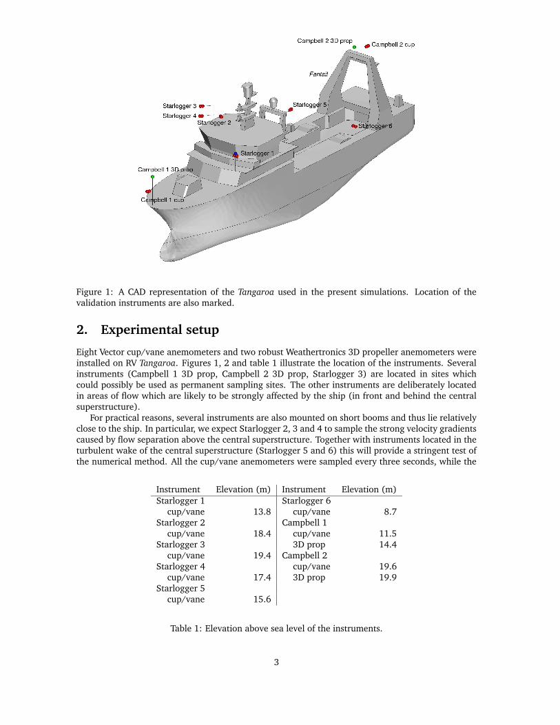
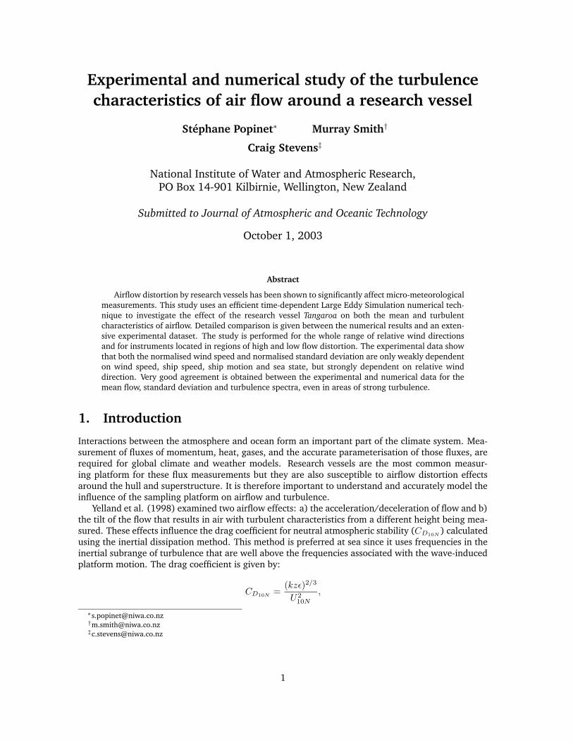
Figure 1: A CAD representation of the Tangaroa used in the present simulations. Location of thevalidation instruments are also marked.

2. Experimental setup

Eight Vector cup/vane anemometers and two robust Weathertronics 3D propeller anemometers wereinstalled on RV Tangaroa. Figures 1, 2 and table 1 illustrate the location of the instruments. Severalinstruments (Campbell 1 3D prop, Campbell 2 3D prop, Starlogger 3) are located in sites whichcould possibly be used as permanent sampling sites. The other instruments are deliberately locatedin areas of flow which are likely to be strongly affected by the ship (in front and behind the centralsuperstructure).

For practical reasons, several instruments are also mounted on short booms and thus lie relativelyclose to the ship. In particular, we expect Starlogger 2, 3 and 4 to sample the strong velocity gradientscaused by flow separation above the central superstructure. Together with instruments located in theturbulent wake of the central superstructure (Starlogger 5 and 6) this will provide a stringent test ofthe numerical method. All the cup/vane anemometers were sampled every three seconds, while the

Instrument Elevation (m) Instrument Elevation (m)

Starlogger 1 Starlogger 6cup/vane 13.8 cup/vane 8.7

Starlogger 2 Campbell 1cup/vane 18.4 cup/vane 11.5

Starlogger 3 3D prop 14.4cup/vane 19.4 Campbell 2

Starlogger 4 cup/vane 19.6cup/vane 17.4 3D prop 19.9

Starlogger 5cup/vane 15.6

Table 1: Elevation above sea level of the instruments.

3

Starlogger 1 Starlogger 2, 3, 4 Starlogger 5

Starlogger 6 Campbell 1 3D prop, cup Campbell 2 3D prop

Figure 2: Individual mountings of instruments marked in figure 1.

4

Figure 3: Side-on wind flow. The stream ribbons and cross-section at sea level are coloured accordingto the norm of the velocity.

3D propellers were sampled at four Hertz.

3. Numerical method

Most CFD programs used for engineering applications provide a solution of the Reynolds averagedNavier-Stokes equations (RANS) where the averaging is carried out in space and time. The solutionobtained is thus a stationary, time-averaged representation of the flow and provides only limitedinformation on the turbulence characteristics. Another possibility is to carry out the averaging onlyspatially. The resulting time-dependent solution is then obtained using methods usually referred toas Large Eddy Simulations (LES). While these methods can be more computationally expensive, theyrequire fewer assumptions for modelling turbulent stresses and have the potential to provide bettersolutions, particularly in wakes or recirculating regions (Shah and Ferziger 1997; Rodi et al. 1997)or around the bluff bodies we are interested in (Baetke et al. 1990; Murakami 1993).

The numerical method we used has been described in detail in Popinet (2003). Its implementationis freely available (Popinet 2002). In the following we summarise the main characteristics of thetechnique.

a. Spatial discretisation

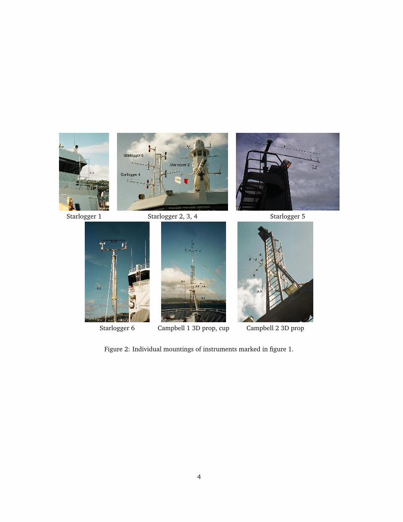
The computational domain is discretised using cubic finite volumes organised as a spatial octree(Samet 1989; Khokhlov 1998). This type of discretisation is very flexible and allows the spatial res-olution to dynamically adapt to follow the evolving flow structures (Popinet 2003). An example ofsuch a discretisation is given in figure 4. The wake created by the ship for a side-on wind flow isresolved using the finest mesh. Far from the ship, only large structures are present and the spa-tial resolution decreases accordingly. The mesh is adapted at each time step to follow the evolvingturbulent boundary of the wake.

This mechanism allows substantial savings in computation time. Fine meshes can thus be used to

5

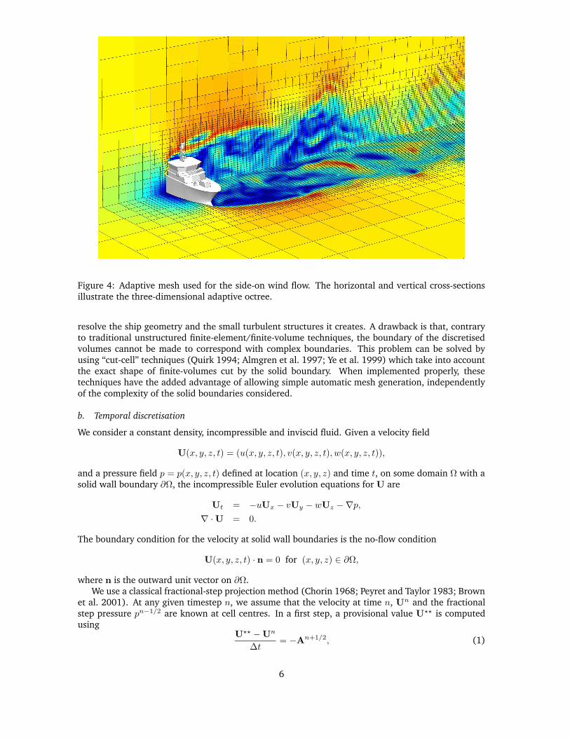
Figure 4: Adaptive mesh used for the side-on wind flow. The horizontal and vertical cross-sectionsillustrate the three-dimensional adaptive octree.

resolve the ship geometry and the small turbulent structures it creates. A drawback is that, contraryto traditional unstructured finite-element/finite-volume techniques, the boundary of the discretisedvolumes cannot be made to correspond with complex boundaries. This problem can be solved byusing “cut-cell” techniques (Quirk 1994; Almgren et al. 1997; Ye et al. 1999) which take into accountthe exact shape of finite-volumes cut by the solid boundary. When implemented properly, thesetechniques have the added advantage of allowing simple automatic mesh generation, independentlyof the complexity of the solid boundaries considered.

b. Temporal discretisation

We consider a constant density, incompressible and inviscid fluid. Given a velocity field

U(x, y, z, t) = (u(x, y, z, t), v(x, y, z, t), w(x, y, z, t)),

and a pressure field p = p(x, y, z, t) defined at location (x, y, z) and time t, on some domain Ω with asolid wall boundary ∂Ω, the incompressible Euler evolution equations for U are

Ut = −uUx − vUy − wUz −∇p,

∇ · U = 0.

The boundary condition for the velocity at solid wall boundaries is the no-flow condition

U(x, y, z, t) · n = 0 for (x, y, z) ∈ ∂Ω,

where n is the outward unit vector on ∂Ω.We use a classical fractional-step projection method (Chorin 1968; Peyret and Taylor 1983; Brown

et al. 2001). At any given timestep n, we assume that the velocity at time n, Un and the fractional

step pressure pn−1/2 are known at cell centres. In a first step, a provisional value U?? is computed

usingU

??− U

n

∆t= −A

n+1/2, (1)

6

where An+1/2 is an approximation to the advection term [(U · ∇)U]n+1/2. The new velocity U

n+1 isthen computed by applying an approximate projection operator to U

?? which also yields the fractionalstep pressure pn+1/2 (Almgren et al. 2000).

The advection term An+1/2 is computed using a second-order, unconditionally stable, Godunov-

type scheme (Bell et al. 1989), with a cell-merging technique for small cut cells (Quirk 1994). Theoverall scheme is thus second-order in space and time.

c. Poisson equation

The projection method relies on the Hodge decomposition of the velocity field as

U?? = U + ∇φ, (2)

where∇ · U = 0 in Ω and U · n = 0 on ∂Ω. (3)

Taking the divergence of (2) yields the Poisson equation

∇2φ = ∇ · U

??, (4)

while the normal component of (3) yields the boundary condition

∂φ

∂n= U

??· n on ∂Ω.

The divergence-free velocity field is then defined as

U = U??

−∇φ,

where φ is obtained as the solution of the Poisson problem (4). This defines the projection of thevelocity U

?? onto the space of divergence-free velocity fields.This projection step is the most expensive part of the solution algorithm because equation (4)

results in a spatially implicit problem (i.e. a linear system of equations for each discrete volume). Weuse an efficient multigrid-accelerated relaxation technique which combines naturally with the octreespatial discretisation (Popinet 2003).

d. Turbulence modelling

Given the very high Reynolds number of a typical airflow around a ship (R ≈ 109) direct numericalsimulations are not feasible: the scale of the smallest possible structures (the Kolmogorov scale) beingof the order of 1/R. Some turbulence modelling is thus necessary to approximate the energy transferat scales smaller than the mesh size. In Large Eddy Simulations (LES) this subgrid energy transfer isusually assumed to take the form of a subgrid turbulent viscous stress where the viscosity coefficient isvariable both in space and time and described using semi-empirical relationships (Lesieur and Metais1996).

As described above, the numerical model we use does not contain any explicit viscous terms. Inpractice numerical schemes always have some numerical viscosity due to higher order errors associ-ated with the discrete representation of the solution. Remarkably, several authors (Boris et al. 1992;Porter et al. 1994) have shown that this numerical dissipation can describe turbulent subgrid energytransfer as well or sometimes better than more complex LES semi-empirical models. Consequently,this first study will not use any explicit turbulent dissipation, while we certainly do intend to investi-gate more complex LES models in the future.

4. Experimental Results

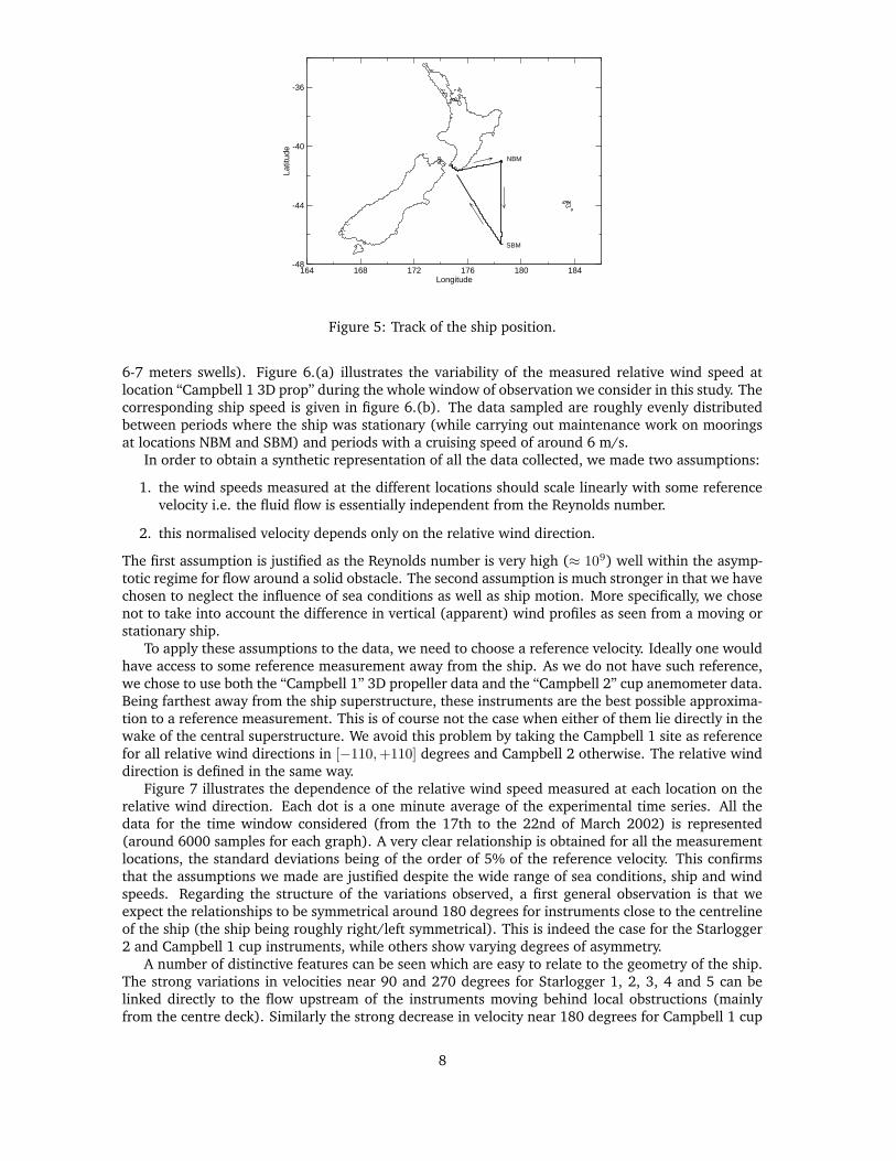
Data was collected continuously during a week long cruise in the Pacific ocean, south-east of theNew Zealand mainland, during March 2002 (see figure 5). A range of wind speeds, up to 20 m/s,was sampled with sea conditions and ship motion varying accordingly (from calm seas to up to

7

164 168 172 176 180 184Longitude

-48

-44

-40

-36

Latit

ude

NBM

SBM

Figure 5: Track of the ship position.

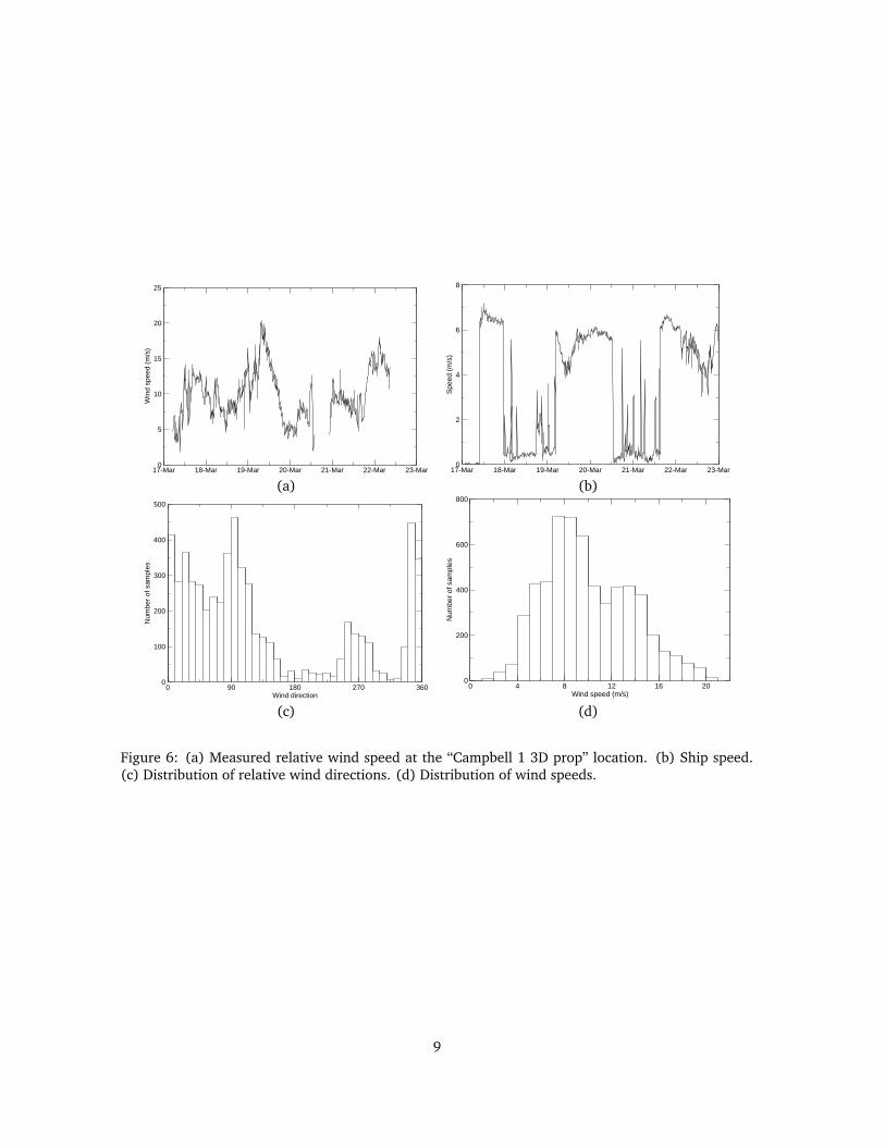
6-7 meters swells). Figure 6.(a) illustrates the variability of the measured relative wind speed atlocation “Campbell 1 3D prop” during the whole window of observation we consider in this study. Thecorresponding ship speed is given in figure 6.(b). The data sampled are roughly evenly distributedbetween periods where the ship was stationary (while carrying out maintenance work on mooringsat locations NBM and SBM) and periods with a cruising speed of around 6 m/s.

In order to obtain a synthetic representation of all the data collected, we made two assumptions:

1. the wind speeds measured at the different locations should scale linearly with some referencevelocity i.e. the fluid flow is essentially independent from the Reynolds number.

2. this normalised velocity depends only on the relative wind direction.

The first assumption is justified as the Reynolds number is very high (≈ 109) well within the asymp-totic regime for flow around a solid obstacle. The second assumption is much stronger in that we havechosen to neglect the influence of sea conditions as well as ship motion. More specifically, we chosenot to take into account the difference in vertical (apparent) wind profiles as seen from a moving orstationary ship.

To apply these assumptions to the data, we need to choose a reference velocity. Ideally one wouldhave access to some reference measurement away from the ship. As we do not have such reference,we chose to use both the “Campbell 1” 3D propeller data and the “Campbell 2” cup anemometer data.Being farthest away from the ship superstructure, these instruments are the best possible approxima-tion to a reference measurement. This is of course not the case when either of them lie directly in thewake of the central superstructure. We avoid this problem by taking the Campbell 1 site as referencefor all relative wind directions in [−110,+110] degrees and Campbell 2 otherwise. The relative winddirection is defined in the same way.

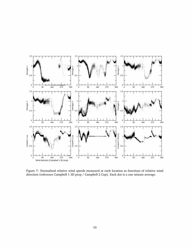
Figure 7 illustrates the dependence of the relative wind speed measured at each location on therelative wind direction. Each dot is a one minute average of the experimental time series. All thedata for the time window considered (from the 17th to the 22nd of March 2002) is represented(around 6000 samples for each graph). A very clear relationship is obtained for all the measurementlocations, the standard deviations being of the order of 5% of the reference velocity. This confirmsthat the assumptions we made are justified despite the wide range of sea conditions, ship and windspeeds. Regarding the structure of the variations observed, a first general observation is that weexpect the relationships to be symmetrical around 180 degrees for instruments close to the centrelineof the ship (the ship being roughly right/left symmetrical). This is indeed the case for the Starlogger2 and Campbell 1 cup instruments, while others show varying degrees of asymmetry.

A number of distinctive features can be seen which are easy to relate to the geometry of the ship.The strong variations in velocities near 90 and 270 degrees for Starlogger 1, 2, 3, 4 and 5 can belinked directly to the flow upstream of the instruments moving behind local obstructions (mainlyfrom the centre deck). Similarly the strong decrease in velocity near 180 degrees for Campbell 1 cup

8

17-Mar 18-Mar 19-Mar 20-Mar 21-Mar 22-Mar 23-Mar0

5

10

15

20

25

Win

d sp

eed

(m/s

)

17-Mar 18-Mar 19-Mar 20-Mar 21-Mar 22-Mar 23-Mar0

2

4

6

8

Spe

ed (

m/s

)

(a) (b)

0 90 180 270 360Wind direction

0

100

200

300

400

500

Num

ber

of s

ampl

es

0 4 8 12 16 20Wind speed (m/s)

0

200

400

600

800

Num

ber

of s

ampl

es

(c) (d)

Figure 6: (a) Measured relative wind speed at the “Campbell 1 3D prop” location. (b) Ship speed.(c) Distribution of relative wind directions. (d) Distribution of wind speeds.

9

0 90 180 270 360

Wind direction (Campbell 1 3D prop)

0

0.5

1

1.5

Cam

pbel

l 1 c

up

0 90 180 270 3600

0.5

1

1.5

Sta

rlogg

er 4

0 90 180 270 3600

0.5

1

1.5

Sta

rlogg

er 1

0 90 180 270 3600

0.5

1

1.5

Cam

pbel

l 2 c

up

0 90 180 270 3600

0.5

1

1.5

Sta

rlogg

er 5

0 90 180 270 3600

0.5

1

1.5

Sta

rlogg

er 2

0 90 180 270 3600

0.5

1

1.5

Cam

pbel

l 2 3

D p

rop

0 90 180 270 3600

0.5

1

1.5

Sta

rlogg

er 6

0 90 180 270 3600

0.5

1

1.5

Sta

rlogg

er 3

Figure 7: Normalised relative wind speeds measured at each location as functions of relative winddirection (reference Campbell 1 3D prop / Campbell 2 Cup). Each dot is a one minute average.

10

can be associated with the instrument being in the wake of the central superstructure. The structureof the dependence for most of the instruments can be characterised by two regimes:

• a more or less “laminar” regime where the instrument sits in a relatively undisturbed flow(possibly with some potential flow acceleration) e.g. Starlogger 1 and 2 between 0 and 75degrees, Starlogger 3 and 4 between 0 and 180 degrees.

• a strongly turbulent regime where the instruments sits downstream of an obstruction e.g. Star-logger 1 and 2 above 90 degrees, Starlogger 3 and 4 between 180 and 270 degrees.

Starlogger 6 is a particular case where only the turbulent regime is present, the instrument almostalways being downstream of some obstruction.

Some features of Campbell 1 cup deserve particular attention. This instrument is located immedi-ately below Campbell 1 3D prop, used as reference for all “bow-on” winds. One would thus expect anearly constant relationship for all bow-on angles, but a sharp decrease is observed around 15 degreesas well as other well-defined structures near 270 degrees. Apart from systematic instrumental errors(improbable given the well-defined features and wide range of wind speeds), a probable explanationis the influence on the measured wind speed of small-scale details like mast mounting and fittings.

5. Comparison with numerical simulations

a. Numerical setup

Using the numerical method previously described we performed a number of simulations of the flowaround a CAD model of RV Tangaroa for different relative wind directions. The CAD model usedis pictured in figure 1. We aimed for a spatial resolution near the ship of around 50 centimetres.Consistently the smallest details represented in the CAD model are of this order. In order to minimisethe influence of the boundary conditions, the CAD model is positioned in a cubic domain 276 metreswide (four times the ship length). The corresponding maximum blockage ratio obtained for beam-onflows is of the order of one percent. A constant, unity inflow velocity is imposed to the left side of thedomain, simple outflow conditions to the right side and slip conditions on all the other boundaries(including the sea surface). As in Dupuis et al (2003), we chose not to impose a more complexvelocity profile (logarithmic boundary layer or other models) at the inflow for two reasons:

1. we solve the Euler equations and thus cannot impose the explicit dissipative terms consistentwith a non-zero stress at the sea surface.

2. the experimental results have shown that the flow distortion is largely independent of the shipmotion and thus of the detail of the vertical wind velocity profile.

The simulations are all started with the potential flow solution as initial conditions. As time passes,the vorticity generated at the solid boundaries (essentially near sharp features of the CAD model) isadvected away from the ship and evolves into a fully developed turbulent wake. The computationalmesh is adapted dynamically to follow this evolution using the vorticity criterion (figure 4). We choseto refine the mesh in areas of high vorticity down to a spatial scale of one metre (50 cm if close tothe ship). Depending on the relative wind direction, between 200,000 and 350,000 grid points werenecessary to resolve the fully developed turbulent wakes.

Typical results are illustrated in figure 8 and 9 for bow-on and stern-on flows respectively. Thepictures are a snapshot in time of the fully-developed wake. The stream ribbons (streamlines twistedaccording to the local vorticity vector) pictured go through individual instrument locations. In figure8 two regimes can be clearly distinguished: a laminar flow upstream of the central superstructureand a strongly turbulent flow downstream. The signature of this turbulent wake is clearly seen inthe large fluctuation in wind velocity near sea level (coloured plane) while the close to potential flowsolution upstream creates the characteristic low wind zone just upstream of the bow.

Since our model is time-dependent, it was necessary to select a window over which to time-average the numerical fields in order to compare the numerical results to the time-averaged experi-mental data of figure 7. We chose to stop the simulations at t? = tU/L = 3 where U is the inflow

11

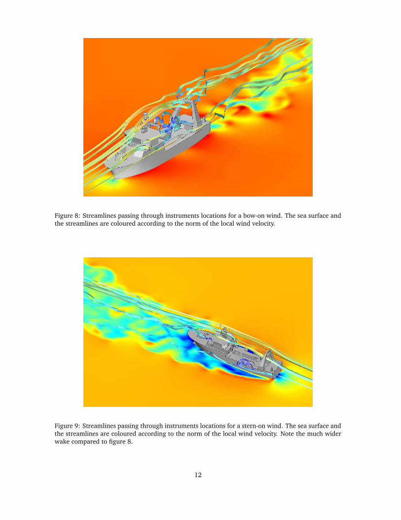
Figure 8: Streamlines passing through instruments locations for a bow-on wind. The sea surface andthe streamlines are coloured according to the norm of the local wind velocity.

Figure 9: Streamlines passing through instruments locations for a stern-on wind. The sea surface andthe streamlines are coloured according to the norm of the local wind velocity. Note the much widerwake compared to figure 8.

12

0 90 180 270 3600

0.5

1

1.5

Cam

pbel

l 1 c

up

0 90 180 270 3600

0.5

1

1.5

Sta

rlogg

er 4

0 90 180 270 3600

0.5

1

1.5

Sta

rlogg

er 1

0 90 180 270 3600

0.5

1

1.5

Cam

pbel

l 2 c

up

0 90 180 270 3600

0.5

1

1.5

Sta

rlogg

er 5

0 90 180 270 3600

0.5

1

1.5

Sta

rlogg

er 2

0 90 180 270 3600

0.5

1

1.5

Cam

pbel

l 2 3

D p

rop

0 90 180 270 3600

0.5

1

1.5

Sta

rlogg

er 6

0 90 180 270 3600

0.5

1

1.5

Sta

rlogg

er 3

Figure 10: Relative wind speeds at each location as functions of relative wind direction. The ex-perimental data is represented by the bounding curves defined by: mean plus or minus standarddeviation. The symbols are the results of numerical simulations.

velocity and L = 276 metres is the domain size, and to time-average the fields for t?∈ [1, 3]. One t?

unit was enough in all cases to obtain a fully-developed turbulent regime from the initial potentialsolution.

b. Mean flow distortion

A series of simulations were performed with a relative wind direction varying from 0 to 360 degreesby increments of 15 degrees. Each simulation took approximately 20 hours of CPU time on a 2 GHzcompatible PC. The results for the time-averaged relative wind speeds calculated at each instrumentlocation are pictured in figure 10 together with the experimental data. For clarity, the experimentaldata of figure 7 is summarised here by the two curves: mean plus or minus standard deviation.

When looking more closely at the results, it is useful to distinguish the laminar and turbulentregimes. Very good agreement between the simulations and the experimental data is obtained in thelaminar regime: 0 to 90 degrees for Starlogger 1 and 2 and 0 to 180 degrees for Starlogger 3 and 4. Inthe turbulent regime, good agreement is still obtained: correct low values for Starlogger 1 between90 and 270 degrees, “M structure” for Starlogger 2, sharp gradients for Starlogger 3, 4 and 5. Asnoted earlier, Starlogger 6 is a difficult case, being located on the lower deck and always in a turbulentregime. While the general trend is reproduced by the model a number of small structures do not seemto match very well. A possible explanation is that several small scale structures (winches, railings,deck crane etc...) close to the instrument location are not represented in the CAD model. Similarly,the small structures in Campbell 1 cup and Campbell 2 cup which we attributed to local perturbations

13

0 90 180 270 360Wind direction

-20

-10

0

10

Ang

le fr

om h

oriz

onta

l (de

gree

)

Campbell 1 3D prop

0 90 180 270 360Wind direction

-10

0

10

20

30

Ang

le fr

om h

oriz

onta

l (de

gree

s)

Campbell 2 3D prop

(a) (b)

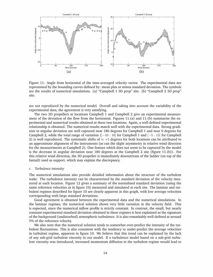
Figure 11: Angle from horizontal of the time-averaged velocity vector. The experimental data arerepresented by the bounding curves defined by: mean plus or minus standard deviation. The symbolsare the results of numerical simulations. (a) “Campbell 1 3D prop” site. (b) “Campbell 2 3D prop”site.

are not reproduced by the numerical model. Overall and taking into account the variability of theexperimental data, the agreement is very satisfying.

The two 3D propellers at locations Campbell 1 and Campbell 2 give an experimental measure-ment of the deviation of the flow from the horizontal. Figures 11.(a) and 11.(b) summarise the ex-perimental and numerical results obtained at these two locations. Again, a well-defined experimentalrelationship is obtained. The numerical results match well with the experimental data. Strong gradi-ents in angular deviation are well captured near 180 degrees for Campbell 1 and near 0 degrees forCampbell 2, while the total range of variation ([−10 : 10] for Campbell 1 and [−5 : 15] for Campbell2) is well reproduced. The systematic shifts of ≈ +5 degrees for both locations can be attributed toan approximate alignment of the instruments (as can the slight asymmetry in relative wind directionfor the measurements at Campbell 2). One feature which does not seem to be captured by the modelis the decrease in angular deviation near 180 degrees at the Campbell 2 site (figure 11.(b)). Forthis relative wind direction, the 3D propeller is immediately downstream of the ladder (on top of thefantail) used as support, which may explain the discrepancy.

c. Turbulence intensity

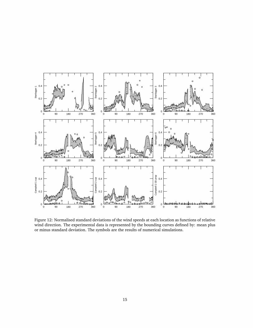
The numerical simulations also provide detailed information about the structure of the turbulentwake. The turbulence intensity can be characterised by the standard deviation of the velocity mea-sured at each location. Figure 12 gives a summary of the normalised standard deviation (using thesame reference velocities as in figure 10) measured and simulated at each site. The laminar and tur-bulent regimes described for figure 10 are clearly apparent in this graph, with low average velocitiescorresponding with large standard deviations.

Good agreement is obtained between the experimental data and the numerical simulations. Inthe laminar regimes, the numerical solution shows very little variation in the velocity field. Thisis expected, since the numerical inflow profile is strictly constant. In contrast, the small, but nearlyconstant experimental standard deviation obtained in these regimes is best explained as the signatureof the background (undisturbed) atmospheric turbulence. It is also remarkably well-defined at around5% of the reference velocity.

We also note that the numerical solution tends to somewhat over-predict the intensity of the tur-bulent fluctuations. This is also consistent with the tendency to under-predict the average velocitiesin turbulent regime, apparent in figure 10. We believe that this trend can be explained by the lackof any sub-grid turbulent viscosity in our model. If a turbulence model based on a sub-grid turbu-lent viscosity was introduced, increased momentum diffusion in the turbulent regime would lead to

14

0 90 180 270 3600

0.2

0.4

Cam

pbel

l 1 c

up

0 90 180 270 3600

0.2

0.4

Sta

rlogg

er 4

0 90 180 270 3600

0.2

0.4

Sta

rlogg

er 1

0 90 180 270 3600

0.2

0.4

Cam

pbel

l 2 c

up

0 90 180 270 3600

0.2

0.4

Sta

rlogg

er 5

0 90 180 270 3600

0.2

0.4

Sta

rlogg

er 2

0 90 180 270 3600

0.2

0.4

Cam

pbel

l 2 3

D p

rop

0 90 180 270 3600

0.2

0.4

Sta

rlogg

er 6

0 90 180 270 3600

0.2

0.4

Sta

rlogg

er 3

Figure 12: Normalised standard deviations of the wind speeds at each location as functions of relativewind direction. The experimental data is represented by the bounding curves defined by: mean plusor minus standard deviation. The symbols are the results of numerical simulations.

15

0.01 0.10 1.00Frequency (Hz)

0.001

0.010

0.100

1.000

10.000

100.000

PS

D (

ms

−1 )2 H

z−1

Propeller FTPropeller FMModel FM

−5/2

Figure 13: Comparison of modelled downwind power spectral density of velocity (solid line) withmeasured spectra upwind (dotted) and downwind (dot-dash). The relative wind speed was 10 m/sfrom astern.

smaller velocity fluctuations and larger average velocities.Another interesting feature of figure 12, when examined together with figure 10 is the correlation

of increased turbulence with the small features seen for the Campbell 1 cup and Campbell 2 cupsites (near 15 and 75, 180 degrees respectively). This tends to confirm our hypothesis that theselocal average velocity variations are caused by small-scale upstream obstructions. The signature of asimilar upstream obstruction, though of larger spatial extend, is clearly seen near 180 degrees for theStarlogger 6 location and is reproduced by the numerical simulation. It corresponds to one of the legsof the fantail moving upstream of the instrument location. This is clearly illustrated by the complexshape of the streamline going through this location for a stern-on wind (figure 9).

d. Turbulence spectra

The standard deviation of the velocity is only an integrated measure of the turbulent energy contentof the signal measured. Being time-dependent, LES simulations give information about the detailedspatial distribution of turbulent structures down to scales comparable with the grid size. Figure 13gives spectra obtained from experimental and numerical time series. The experimental spectra werecalculated from segments of 1024 points averaged over 30 minutes. Two experimental locationsare used: the foremast 3D propeller (Campbell 1 3D prop) and the fantail propeller (Campbell 23D prop). Controlled comparisons between a sonic anemometer and the propellers showed that theresponse of the propellers starts to roll off above 0.4 Hz, in keeping with early studies of these in-struments (Horst 1973). For this comparison we deliberately chose the difficult situation of turbulentairflow in the wake of the vessel with the wind almost directly astern (165 degrees).

It is clear that the total energy content of the measured downwind turbulent spectrum exceeds theupwind spectrum by at least a factor of 6, indicating that the turbulent wake intensity significantlyexceeds the background atmospheric turbulence intensity (which is consistent with the standard de-viation data of figure 12/Campbell 1 cup). The modelled wake spectrum agrees very well with the

16

Figure 14: Isosurface at 90% of the time-averaged wind velocity for a bow-on flow. The velocityinside the volume pictured is lower than 90% of the inflow velocity.

Figure 15: Isosurface at 25% of the normalised standard deviation for a bow-on flow. The standarddeviation of the velocity inside the volume pictured is larger than 25% of the inflow velocity.

measured spectrum both qualitatively and quantitatively. The modelled spectrum does show a fasterfalloff above 1 Hz which we attribute to the finite spatial resolution of the model. Further model runsat higher resolution (not shown) extended the cutoff region to higher frequencies as expected (??).The modelled spectrum peaks at 0.15 Hz, corresponding to a dominant eddy scale size of ≈66 mwhich is close to the scale size of the ship length. The modelled fall-off at lower frequencies indicatesthat no spatial structures larger than the ship length are created. This is consistent with vortex shed-ding occurring at scales comparable to the ship length and then decaying into smaller structures. Atlow frequencies (below 0.05 Hz) the upwind and downwind experimental spectra converge indicat-ing that at the corresponding length scales the influence of the ship on the background atmosphericturbulence is negligible. In the 0.04-0.2 Hz frequency range, ship motion (more particularly changesin relative wind direction due to yaw) typically have a strong influence on the measured spectrum.

e. General characteristics

One of the strength of the numerical simulations is that they give a global picture of the flow structurewhich is difficult to infer from point measurements. Three-dimensional maps characterising variousmeasures of flow distortion are easily obtained. As an example, figure 14 uses an isosurface at 90%of the time-averaged velocity to illustrate the 3D structure of the velocity field. The large pressurebuilding up at the bow and in front of the central superstructure creates the two rounded low-velocityzones in these areas. These two features would be described by a laminar potential flow approxima-tion. Most of the other features are linked to vorticity generation at the ship boundary and subsequentadvection by the flow. Particularly noticeable features are: the wake of the whole ship extending farinto the domain, the wake created by the crow’s nest and a tubular structure starting near the bowand extending the whole length of the ship. Closer examination reveals that this low velocity zonecorresponds to the core of a longitudinal vortex fed by the strong vorticity generation near the bow.

17

Figure 16: Isosurface at 25% of the normalised standard deviation for a 45 degrees wind flow. Thestandard deviation of the velocity inside the volume pictured is larger than 25% of the inflow velocity.

Using only figure 14, it is difficult to gauge of the velocity fluctuations, although one might guessthat the downstream wake is turbulent while the upstream part of the flow is more or less stationary.Figure 15 uses the same type of representation but for the normalised standard deviation. A clearqualitative and quantitative picture of the strongly turbulent wake just downstream of the ship isobtained. It is interesting to note that, while the wake extends very far from the ship as seen onfigure 14, the fluctuations tend to decrease rapidly when the distance to the ship increases. It is alsoseen that the bow vortices described in figure 14 are not associated with any significant fluctuationin velocity (i.e. they are stationary).

Figure 16 is a similar representation but for a 45 degrees relative wind direction. A much widerturbulent wake is generated with several clearly defined sub-wakes linked to specific parts of the ship.Particularly interesting is the strongly turbulent bow wake.

f. Application to micro-meteorological measurements

Figure 17.(a) and 17.(b) illustrate a characterisation of flow distortion at location “‘Campbell 1 3Dprop” which is the main location used for micro-meteorological measurements on the Tangaroa. Boththe full LES solution and the initial potential flow solution are given. Figure 17.(a) gives the relativevertical displacement of a parcel of air reaching the measurement location as a function of relativewind direction. This value is computed from the numerical results by following the time-averagedstreamline passing through the instrument location. The vertical displacement of 1.5 meters for abow-on flow and 6 meters for a 90 degrees relative wind direction are comparable to results obtainedby (Yelland et al. 1998, 2002). Figure 17.(b) illustrates the dependence in relative wind direction ofthe wind speed measured relative to the inflow (exact) wind speed. The obstruction by the ship fora bow-on flow causes an under-estimation of 7% of the wind speed, while for a 90 degrees relativewind direction the wind speed is over-estimated by 10%. These corrections will be applied to thedetermination of CD in future work. It is interesting to note that, while the potential flow solutiongives a reasonable prediction of the relative wind speed for bow-on flows, it severely under-predictsthe elevation for all relative wind directions.

The experiments carried out on the Tangaroa have validated the ability of the Gerris CFD model to

18

0 90 180 270 360Wind angle

0

2

4

6

8

10

12

Ver

tical

dis

plac

emen

t (m

)

Potential flowLES model

0 90 180 270 360Wind angle

0.5

0.6

0.7

0.8

0.9

1

1.1

1.2

Rel

ativ

e w

ind

spee

d

LES modelPotential flow

(a) (b)

Figure 17: Characterisation of flow distortion at location “Campbell 1 3D prop”. (a) Vertical displace-ment. (b) Relative wind speed.

simulate both time-averaged flow and time-varying turbulent structure. We are now able to considerspecific problems relating to both the generation and distortion of turbulence by flow disturbance. Inparticular the region in front of the bow has been used as a gas flux profiling site in several recentexperiments (e.g. (McGillis et al. 2001)), yet it is subject to effects due to pressure build up as shownin figure 14. We are now confident that the CFD model can be used to examine the effect of the shipon turbulent transfer at this location. This will be the subject of further study.

6. Conclusion

The experimental data set collected as part of this study confirms that the mean flow characteristicsare only weakly dependent on ship motion, ship speed, wind speed or sea state, but strongly de-pendent on the relative wind direction. A new finding is that the normalised wind speed standarddeviation (square-root of the turbulent kinetic energy) is also well characterised as a function of rel-ative wind direction only. The standard deviation of the background atmospheric flow measured bywell-exposed instruments is consistently close to 5% of the incoming wind speed. For badly exposedinstruments, located in the wake of the ship superstructure, normalised standard deviations as high as40% can be observed. The experimental data also confirm that even quite small structural elements(such as instruments mountings) can cause significant flow distortion.

Numerical studies performed using our time-dependent LES code show a very good agreementwith both experimental mean velocities and standard deviations. These results have been obtainedfor the whole range of relative wind directions (from bow-on to stern-on) and remain valid in zonesof high turbulence and high flow distortion. We also made use of the time-dependent nature of LESto obtain turbulence spectra. They are in excellent agreement with experimental data. The adaptivemesh technique we use has thus proved to give fast and accurate solutions for turbulent flows. Thesesolutions are particularly useful when a global understanding of the flow pattern is sought, in orderfor example to optimise sampling location. The results also provide correction factors which can beapplied to calculations of drag coefficients.

This work provides a validated basis for future studies. Although promising, the spectral analysispresented here is only preliminary and relies on a limited experimental dataset due to technicalconstraints (low sampling rates and high response time of most of the anemometers used). In thefuture we intend to carry out a more extensive measurement campaign using sonic anemometers.From a numerical modelling perspective, the simulation of turbulent flows around bluff bodies is stillvery much a work in progress in need of improvements (Shah and Ferziger 1997; Rodi et al. 1997;Iacacarino et al. 2003). Finally, by providing an open source version of the code which can be freelyredistributed and modified (Popinet 2002), we hope to encourage research and collaboration in thisfield.

19

References

Almgren, A. S., J. B. Bell, P. Colella, and T. Marthaler, 1997: A Cartesian grid projection method forthe incompressible Euler equations in complex geometries. SIAM J. Sci. Comp., 18.

Almgren, A. S., J. B. Bell, and W. Y. Crutchfield, 2000: Approximate projection methods: Part I.Inviscid analysis. SIAM Journal on Scientific Computing, 22, 1139–1159.

Baetke, F., H. Werner, and H. Wengle, 1990: Numerical simulation of turbulent flow over surface-mounted obstacles with sharp edges and corners. J. Wind Eng. Ind. Aero., 35, 129–147.

Bell, J. B., P. Colella, and H. M. Glaz, 1989: A second-order projection method for the incompressibleNavier-Stokes equations. J. Comput. Phys., 85, 257–283.

Boris, J. P., F. F. Grinstein, E. S. Oran, and R. L. Kolbe, 1992: New insights into large-eddy simulation.Fluid Dyn. Res., 199–228.

Brown, D. L., R. Cortez, and M. L. Minion, 2001: Accurate projection methods for the incompressibleNavier-Stokes equations. J. Comput. Phys., 168, 464–499.

Brut, A., A. Butet, S. Planton, P. Durand, and G. Caniaux: 2002, Influence of the airflow distortionon air-sea flux measurements aboard research vessel: results of physical simulations applied to theEqualant99 experiment. 15th AMS Conf. Boundary Layer & Turbulence, Wageningen, Netherlands.

Chorin, A. J., 1968: Numerical solution of the Navier-Stokes equations. Math. Comp., 22, 745–762.

Dupuis, H., C. Guerin, D. Hauser, A. Weill, P. Nacass, W. Drennan, S. Cloch, and H. Graber, 2003: Im-pact of flow distortion corrections on turbulent fluxes estimated by the inertial dissipation methodduring the FETCH experiment on R/V L’Atalante. J. Geophys. Res., C3.

Horst, T. W., 1973: Corrections for response errors in a three-component propeller anemometer. J.

Appl. Meteorol., 12, 716–725.

Iacacarino, G., A. Ooi, P. A. Durbin, and M. Behnia, 2003: Reynolds averaged simulation of unsteadyseparated flow. Int. J. Heat and Fluid Flow, 24, 147–156.

Kahma, K. K. and M. Lepparanta, 1981: On errors in wind speed observations on R/V Aranda. Geo-

physica, 17, 155–165.

Khokhlov, A. M., 1998: Fully threaded tree algorithms for adaptive refinement fluid dynamics simu-lations. J. Comput. Phys., 143, 519–543.

Lesieur, M. and O. Metais, 1996: New trends in large-eddy simulations of turbulence. Ann. Rev. Fluid

Mech., 28, 45–82.

McGillis, W. R., J. B. Edson, J. D. Ware, J. W. H. Dacey, J. E. Hare, C. W. Fairall, and R. Wanninkhof,2001: Carbon dioxide flux techniques performed during GasEx-98. Marine Chemistry, 75, 267–280.

Murakami, S., 1993: Comparison of various turbulence models applied to a bluff body. J. Wind Eng.

Ind. Aero., 46, 21–36.

Oost, W. A., C. Fairall, J. Edson, S. Smith, R. Anderson, J. Wills, K. Katsaros, and J. DeCosmo, 1994:Flow distortion calculations and their application in HEXMAX. J. Atmos. Oceanic Technol., 11, 366–386.

Pedreros, R., G. Dardier, H. Dupuis, H. Graber, W. Drennan, A. Weill, C. Guerin, and P. Nacass: 2003,Momentum and heat fluxes via the eddy correlation method on the R/V L’Atalante and an Asis buoy,submitted to J. Geophys. Res.

Peyret, R. and T. D. Taylor, 1983: Computational Methods for Fluid Flow. Springer Verlag, NewYork/Berlin.

20

Popinet, S., 2002: The Gerris Flow Solver. http://gfs.sourceforge.net.

— 2003: Gerris: a tree-based adaptive solver for the incompressible Euler equations in complexgeometries. J. Comp. Phys., 190, 572–600.

Porter, D. H., A. Pouquet, and P. R. Woodward, 1994: Kolmogorov-like spectra in decaying three-dimensional supersonic flows. Phys. Fluids, 6, 2133–2142.

Quirk, J. J., 1994: An alternative to unstructured grids for computing gas dynamics flows aroundarbitrarily complex two-dimensional bodies. Computers and Fluids, 23, 125–142.

Rodi, W., J. H. Ferziger, M. Breuer, and M. Pourquie, 1997: Current status of large-eddy simulations:results of a workshop. ASME J. Fluids Eng., 119, 248–262.

Samet, H., 1989: Applications of Spatial Data Structures. Addison-Wesley Publishing Company.

Shah, K. B. and J. H. Ferziger, 1997: A fluid mechanician’s view of wind engineering: large-eddysimulation of flow past a cubical obstacle. J. Wind Eng. Ind. Aero., 67/68, 211–224.

Thiebaux, M. L., 1990: Wind tunnel experiments to determine correction functions for shipborneanemometers. Canadian Contractor Report of Hydrography and Ocean Sciences 36. Technical re-port, Beford Institute of Oceanography, Dartmouth, NS, Canada.

Ye, T., R. Mittal, H. S. Udaykumar, and W. Shyy, 1999: An accurate cartesian grid method for viscousincompressible flows with complex immersed boundaries. J. Comp. Phys., 156, 209–240.

Yelland, M., B. Moat, R. Pascal, and D. Berry, 2002: CFD model estimates of the airflow distortionover research ships and the impact on momentum flux measurements. J. Atmos. Oceanic Technol.,19, 1477–1499.

Yelland, M., B. Moat, P. Taylor, R. Pascal, J. Hutchings, and V. Cornell, 1998: Wind stress measure-ments from the open ocean corrected for airflow distortion by the ship. J. Phys. Oceanogr., 28,1511–1526.

21