Experimental and numerical studies of an eastward...

J. Fluid Mech. (2001), vol. 438, pp. 129–157. Printed in the United Kingdom

c© 2001 Cambridge University Press

129

Experimental and numerical studies of aneastward jet over topography

By Y U D O N G T I A N1, E R I C R. W E E K S2†, K A Y O I D E1,J. S. U R B A C H2‡, C H A R L E S N. B A R O U D2,

M I C H A E L G H I L1¶ AND H A R R Y L. S W I N N E Y2

1Department of Atmospheric Sciences and Institute of Geophysics and Planetary Physics,University of California, Los Angeles, CA 90095, USA

2Center for Nonlinear Dynamics and Department of Physics, University of Texas at Austin,Austin, TX 78712, USA

(Received 8 October 1999 and in revised form 24 October 2000)

Motivated by the phenomena of blocked and zonal flows in Earth’s atmosphere, weconducted laboratory experiments and numerical simulations to study the dynamicsof an eastward jet flowing over wavenumber-two topography. The laboratory experi-ments studied the dynamical behaviour of the flow in a barotropic rotating annulusas a function of the experimental Rossby and Ekman numbers. Two distinct flowpatterns, resembling blocked and zonal flows in the atmosphere, were observed topersist for long time intervals.

Earlier model studies had suggested that the atmosphere’s normally upstream-propagating Rossby waves can resonantly lock to the underlying topography, andthat this topographic resonance separates zonal from blocked flows. In the annulus,the zonal flows did indeed have super-resonant mean zonal velocities, while theblocked flows appear subresonant. Low-frequency variability, periodic or irregular,was present in the measured time series of azimuthal velocity in the blocked regime,with dominant periodicities in the range of 6–25 annulus rotations. Oscillations havealso been detected in zonal states, with smaller amplitude and similar frequency.In addition, over a large region of parameter space the two flow states exhibitedspontaneous, intermittent transitions from the one to the other.

We numerically simulated the laboratory flow geometry in a quasi-geostrophicbarotropic model over a similar range of parameters. Both flow regimes, blockedand zonal, were reproduced in the simulations, with similar spatial and temporalcharacteristics, including the low-frequency oscillations associated with the blockedflow. The blocked and zonal flow patterns are present over wide ranges of forcing,topographic height, and bottom friction. For a significant portion of parameter space,both model flows are stable. Depending on the initial state, either the blocked orthe zonal flow is obtained and persists indefinitely, showing the existence of multipleequilibria.

† Present address: Physics Department, Emory University, Atlanta, GA 30322, USA.‡ Present address: Department of Physics, Georgetown University, Washington, DC 20057, USA.¶ Author to whom correspondence should be addressed.

130 Y. Tian and others

1. Introduction and motivation

The interaction of rotating flows with underlying topography is a classic topicof geophysical fluid dynamics (Gill 1982; Pedlosky 1987). Various applications tothe atmosphere of Earth (Charney & Eliassen 1949; Bolin 1950), Mars (Keppenne& Ingersoll 1995) and Jupiter (Dowling & Ingersoll 1989), as well as to Earth’soceans (Holloway 1992) have been worked out. We are motivated here primarilyby the potential role of such interactions in the Earth atmosphere’s low-frequencyvariability, but expect some of our results to also apply to other areas of geophysicalfluid dynamics.

Because of its important role in the understanding of the general circulation of theatmosphere and in extended-range weather forecasting, low-frequency variability oflarge-scale atmospheric flows has been documented and studied for over fifty years.In particular, since the late 1930s meteorologists have recognized that the large-scaleflow in the Northern Hemisphere alternates between two distinct states, called high-index and low-index flows; the former is characterized by a zonally straight andfaster jet stream and the latter by a wavier and slower one. Such an oscillation tendsto have a more or less regular cycle of 4–6 weeks, and is called the index cycle(Rossby 1939; Namias 1950; Webster & Keller 1975). Blocking (Rex 1950a, b) playsan important role in low-index flows; it involves a strong high-pressure ridge thatappears at preferred locations mostly during the winter, and blocks the normallyzonal flow. A regional block can last for 10–30 days, with substantial impact onlarge-scale weather patterns (O’Connor 1963; Weeks et al. 1997).

During the 1970s and 1980s, subtler low-frequency atmospheric phenomena werediscovered and studied extensively. Among them are the low-frequency oscillationswith periods of 40–50 days, which were first detected in tropical convection andzonal winds (Madden & Julian 1971, 1972), and were also found later by analysis oflength-of-day and atmospheric angular momentum data (Langley, King & Shapiro1981). More detailed observational studies (Anderson & Rosen 1983; Dickey, Ghil &Marcus 1991) have identified a significant contribution to such oscillations from theNorthern Hemisphere extratropics.

Considerable efforts have been devoted to studying the dynamics of these low-frequency phenomena and their underlying relationships. In a barotropic model,Charney & DeVore (1979) obtained multiple equilibria resulting from the nonlinearinteractions between large-scale mid-latitude flow and the underlying topography.The two stable states so obtained had certain features in common with blockedand zonal, or low-index and high-index states in the atmosphere (Charney & Straus1980; Charney, Shukla & Mo 1981). Subsequent studies using various analytical andnumerical models (e.g. Hart 1979; Pedlosky 1981; Legras & Ghil 1985; Yoden 1985;Ghil & Childress 1987, Chap. 6) yielded either multiple equilibria or multiple flowregimes, and highlighted the role of topography in the dynamics of such flows. Someof these studies also obtained low-frequency oscillations, associated with one or all ofthe stationary flow solutions (Charney & DeVore 1979; Legras & Ghil 1985; Yoden1985; Ghil 1987; Strong, Jin & Ghil 1993), and speculated that such oscillationsmay be related to the 40–50-day oscillations observed in the Northern Hemisphereextratropics (Ghil & Mo 1991).

Laboratory studies that model atmospheric phenomena have also played an im-portant role in our understanding of planetary-flow dynamics since the early stagesof the atmospheric sciences. Several rotating annulus experiments have previously in-vestigated the index cycle, blocking, and low-frequency oscillations (Pfeffer & Chiang

Eastward jet over topography 131

1967; Li, Kung & Pfeffer 1986; Pfeffer, Kung & Li 1989; Bernardet et al. 1990; Jonas1981; Pfeffer et al. 1990). Introducing wavenumber-two topography in such annuliproduced new phenomena, such as large-scale standing waves and low–frequencyvacillations associated with them, but did not adequately explain the spatio-temporalfeatures of the atmosphere’s observed and modelled low-frequency variability.

Those experiments used baroclinic annuli with thermal forcing. Low-frequencyatmospheric dynamics is, however, predominantly barotropic (Wallace & Blackmon1983; Marcus, Ghil & Dickey 1994, 1996), and so direct simulation and investigationof barotropic dynamics is desirable for studying those phenomena (Lorenz 1972). Lau& Nath (1987) have shown that the larger the time scale, the more barotropic the flowbecomes. Furthermore, the complications that arise from the fully three-dimensionalstructure of the flows in the baroclinic annuli make the analysis of the experimentalresults more difficult and hinder direct comparisons with existing theoretical resultsand atmospheric observations. Finally, because the forcing mechanism in those ex-periments was through differential heating of the sidewalls, large Reynolds numbersare difficult to achieve and thus the parameter range is limited.

Several barotropic experiments with topography were conducted (Carnevale, Kloost-erziel & van Heijst 1991; Pratte & Hart 1991; Pfeffer et al. 1993) but did not examinequestions of blocking and zonal patterns. Streamfunction fields shown in Pfefferet al. (1993) resemble some of our flow patterns here (see § 2), but the Rossbynumbers for these experiments were very low and the flows examined were alwaystime-independent. The general theory of rotating flow over topography (Queney 1947;Ghil & Childress 1987; Pedlosky 1987; Smith 1989; Wurtele, Sharman & Datta 1996),on the other hand, suggests topographic effects on barotropic flow could be quitesignificant and thus lead to multiple equilibria, as well as to time-dependent flows,even in the presence of constant forcing.

In the present paper we report on experimental results obtained for barotropicflow in a rotating annulus; the flow is driven through concentric rings of holes in thebottom, using a mechanical pump. This generates an eastward jet, and we investigatethe interactions of this jet with two symmetrically placed mountains on the bottom ofthe annulus. We observe two distinct flow patterns, analogous to high- and low-indexflows in the atmosphere. For moderate to high pumping rates, these flows exhibitlow-frequency oscillations, with different oscillatory features being associated withdifferent flows. We also observed spontaneous transitions between these two flowregimes.

The experiment uses a much-simplified laboratory model of Earth’s atmosphere.Our fluid is isothermal and incompressible, and the rigid side, top, and bottom wallsof our annular container differ from the atmosphere’s boundaries. To help understandthe laboratory results and connect them with numerical models of the atmosphere(Charney & DeVore 1979; Pedlosky 1981; Legras & Ghil 1985; Jin & Ghil 1990)and with observations (Dickey et al. 1991; Ghil & Mo 1991; Lott, Robertson &Ghil 2001), we constructed a numerical model to simulate the annulus experiment.The model is governed by the quasi-geostrophic (QG) barotropic potential vorticityequation (e.g. Charney & DeVore 1979; Marcus & Lee 1998; Pedlosky 1987 Chap.4), with forcing and mountains similar to those in the experiment. The values of theparameters in the model are derived directly from the laboratory measurements. Theflow patterns and time dependence obtained in the model agree qualitatively withthose in the experiments, for equivalent parameter values. Furthermore, we use themodel to investigate the influence of topographic height and bottom friction on thedynamics, since these parameters are difficult to vary in the laboratory experiments.


Video camera(a)

H

r2r1

I O Od 2d d

I

(b)

Figure 1. (a) The rotating annulus and (b) the bottom topography. The inner radius is r1 = 10.8 cmand the outer radius is r2 = 43.2 cm; the depth of the annulus increases from 17.1 cm at r1 to 20.3 cmat r2. The angular extent of each of the two mountains is 1.25 rad. The arrows below the tank in(a) show the direction of the inflow (I) and outflow (O) through the holes in the bottom. See textfor other details.

The experimental results of this research are presented in § 2. The numericalinvestigation is reported in § 3. In § 4 we summarize the results and compare thelaboratory results and the computer simulations, and discuss the implications forEarth’s atmosphere.

2. Experimental investigation2.1. Apparatus and experimental design

The experimental apparatus consists of a large rotating annulus, shown schematicallyin figure 1 (Solomon, Holloway & Swinney 1993; Weeks et al. 1997). The top isrigid and flat, and the bottom is rigid and conical with a constant radial slopes = 0.1, to simulate the β-effect. The tank is filled with water, of kinematic viscosityν = 0.0090 cm2 s−1, and can rotate at speeds up to Ω = 8π rad s−1.

Two symmetric, rigid mountains are overlaid on the tank’s conical bottom, tosimulate the dominant topographic component in Earth’s Northern Hemisphere(Charney & Eliassen 1949; Peixoto, Saltzman & Teweles 1964; Legras & Ghil 1985).Above the conical bottom, each mountain has a Gaussian profile along the azimuthaldirection, and is flat along the radial direction; thus each mountain’s surface isdescribed by

h(r, θ) = h0 exp (−θ2/θ20), (2.1)


where r is the radius measured from the centre of the annulus, θ is the azimuthalangle measured from the centreline of the mountain, h0 = 1.5 cm is the maximumheight of both mountains, and θ0 = 0.37 rad. Each mountain extends over 1.25 rad,and its two radial side edges are smoothly tapered from the Gaussian profile of (2.1)to zero to meet the bottom.

To form a jet in the tank, two concentric rings of small holes were drilled throughthe bottom and the mountains, located at rsink = 1.75r1 and rsource = 3.25r1. Theseforcing rings each have 120 holes of 0.26 cm in diameter. A pump forces fluid intothe tank at the outer ring and removes fluid at the inner ring at a constant flow rateF . Due to the counter-clockwise rotation of the annulus, the action of the Coriolisforce deflects the otherwise radial flow into a co-rotating, ‘eastward’ jet.

To observe the flows obtained in the experiment, we use a particle-tracking techniquedue to Pervez & Solomon (1994). Neutrally buoyant particles, 1.0 mm in diameter,are added to the fluid. A 2 cm tall horizontal layer of fluid at the tank’s mid-depth is illuminated from the side, and viewed from a co-rotating video cameraabove the experiment. The images from the video camera are stored in a computer,post-processed to track individual particles, and the time-averaged velocity field isextracted from these data. The corresponding streamfunction field is calculated bya least-squares technique that uses 9 spectral modes in the radial direction and 43spectral modes in the azimuthal direction.

Additionally, to collect more precise information about the velocity fluctuations,we use two hot-film probes. These two probes are placed inside the tank at thesame horizontal position, shown in figure 2, at the channel’s mid-radius, r = 2.5r1,about 15 upstream of one of the mountains. The sensors are oriented to measurethe azimuthal component of the flow velocity, and one is placed approximately 1 cmbelow the top lid and the other 1 cm above the bottom. This allows us to examine thevertical structure of the flow at this horizontal position, and confirm its predominantlytwo-dimensional, barotropic character.

We explored the flows over a wide range of parameters. For each combination ofparameter values, we carried out several runs with different initial states.

2.2. Experimental results

2.2.1. Control parameters and two-dimensionality of the flow

We have two independent control parameters, the forcing flow rate F and theangular velocity Ω of the tank: the pump flux rate F ranges from 0 to 400 cm3 s−1, therotation rate Ω from 1.5π to 3π rad s−1. The forcing is measured by a non-dimensionalRossby number, given by

Ro =U

fL, (2.2)

where L is the spacing between the forcing rings, L = rsource − rsink = 1.5r1 = 16.2 cm;U is the characteristic velocity of the flow; and f = 2Ω is the Coriolis parameter. Theactual velocity of the fluid depends, of course, on the flow regime. Previously (Weekset al. 1997), we chose U to be the maximum velocity that would result from a steady,axisymmetric flow in the absence of topography (Legras & Ghil 1985; Sommeria,Meyers & Swinney 1991),

Umax = (F/2π)(Ω/ν)1/2r−1sink. (2.3)


(a) (b)

Rotation

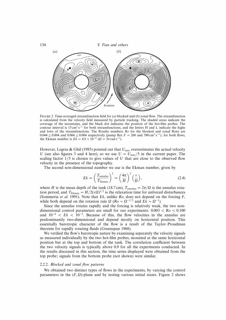
Figure 2. Time-averaged streamfunction field for (a) blocked and (b) zonal flow. The streamfunctionis calculated from the velocity field measured by particle tracking. The shaded areas indicate thecoverage of the mountains, and the black dot indicates the position of the hot-film probes. Thecontour interval is 15 cm2 s−1 for both streamfunctions, and the letters H and L indicate the highsand lows of the streamfunctions. The Rossby numbers Ro for the blocked and zonal flows are0.044 ± 0.004 and 0.066 ± 0.004 respectively (pump flux F = 260 and 390 cm3 s−1); for both flows,the Ekman number is Ek = 4.8× 10−4 (Ω = 3π rad s−1).

However, Legras & Ghil (1985) pointed out that Umax overestimates the actual velocityU (see also figures 3 and 4 here), so we use U = Umax/5 in the current paper. Thescaling factor 1/5 is chosen to give values of U that are close to the observed flowvelocity in the presence of the topography.

The second non-dimensional number we use is the Ekman number, given by

Ek =

(Tannulus

TEkman

)2

=

(4π

H

)2 ( νΩ

), (2.4)

where H is the mean depth of the tank (18.7 cm), Tannulus = 2π/Ω is the annulus rota-tion period, and TEkman = H/2(νΩ)1/2 is the relaxation time for unforced disturbances(Sommeria et al. 1991). Note that Ek, unlike Ro, does not depend on the forcing F ,while both depend on the rotation rate Ω (Ro ∼ Ω−1/2 and Ek ∼ Ω−1).

Since the annulus rotates rapidly and the forcing is relatively weak, the two non-dimensional control parameters are small for our experiments: 0.003 < Ro < 0.100and 10−4 < Ek < 10−3. Because of this, the flow velocities in the annulus arepredominantly two-dimensional and depend mostly on horizontal position. Thisessentially barotropic character of the flow is a result of the Taylor–Proudmantheorem for rapidly rotating fluids (Greenspan 1968).

We verified the flow’s barotropic nature by examining separately the velocity signalsas measured individually by the two hot-film probes, mounted at the same horizontalposition but at the top and bottom of the tank. The correlation coefficient betweenthe two velocity signals is typically above 0.9 for all the experiments conducted. Inthe results discussed in this section, the time series displayed were obtained from thetop probe; signals from the bottom probe (not shown) were similar.

2.2.2. Blocked and zonal flow patterns

We obtained two distinct types of flows in the experiments, by varying the controlparameters in the (F,Ω)-plane and by testing various initial states. Figure 2 shows


10

5

0

–5

–20 –10 0 10 20

(a)

(b)

10

5

0–20 –10 0 10 20

15

r–r0 (cm)

Uh

(cm

s–1

)U

h (c

m s

–1)

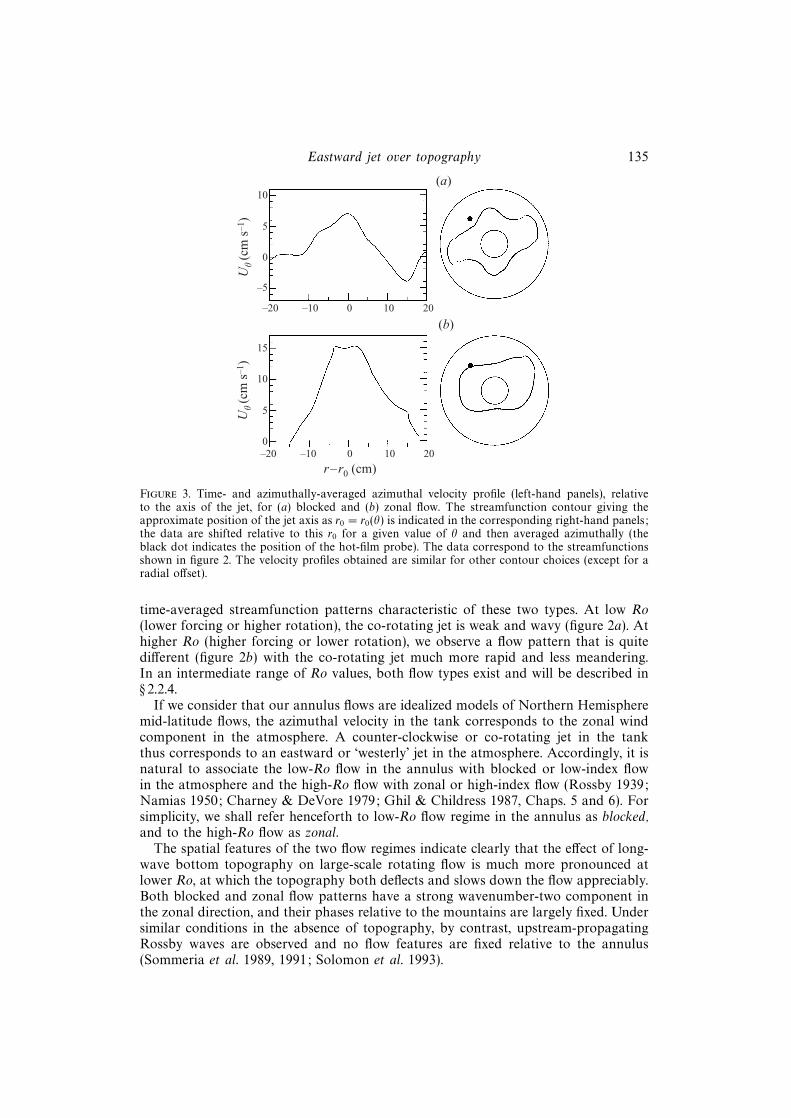
Figure 3. Time- and azimuthally-averaged azimuthal velocity profile (left-hand panels), relativeto the axis of the jet, for (a) blocked and (b) zonal flow. The streamfunction contour giving theapproximate position of the jet axis as r0 = r0(θ) is indicated in the corresponding right-hand panels;the data are shifted relative to this r0 for a given value of θ and then averaged azimuthally (theblack dot indicates the position of the hot-film probe). The data correspond to the streamfunctionsshown in figure 2. The velocity profiles obtained are similar for other contour choices (except for aradial offset).

time-averaged streamfunction patterns characteristic of these two types. At low Ro(lower forcing or higher rotation), the co-rotating jet is weak and wavy (figure 2a). Athigher Ro (higher forcing or lower rotation), we observe a flow pattern that is quitedifferent (figure 2b) with the co-rotating jet much more rapid and less meandering.In an intermediate range of Ro values, both flow types exist and will be described in§ 2.2.4.

If we consider that our annulus flows are idealized models of Northern Hemispheremid-latitude flows, the azimuthal velocity in the tank corresponds to the zonal windcomponent in the atmosphere. A counter-clockwise or co-rotating jet in the tankthus corresponds to an eastward or ‘westerly’ jet in the atmosphere. Accordingly, it isnatural to associate the low-Ro flow in the annulus with blocked or low-index flowin the atmosphere and the high-Ro flow with zonal or high-index flow (Rossby 1939;Namias 1950; Charney & DeVore 1979; Ghil & Childress 1987, Chaps. 5 and 6). Forsimplicity, we shall refer henceforth to low-Ro flow regime in the annulus as blocked,and to the high-Ro flow as zonal.

The spatial features of the two flow regimes indicate clearly that the effect of long-wave bottom topography on large-scale rotating flow is much more pronounced atlower Ro, at which the topography both deflects and slows down the flow appreciably.Both blocked and zonal flow patterns have a strong wavenumber-two component inthe zonal direction, and their phases relative to the mountains are largely fixed. Undersimilar conditions in the absence of topography, by contrast, upstream-propagatingRossby waves are observed and no flow features are fixed relative to the annulus(Sommeria et al. 1989, 1991; Solomon et al. 1993).


The azimuthal flux carried by the zonal flows is typically 3 times larger than inthe blocked case for the same pumping and rotation rates (not shown). The blockedflow shown in figure 2 (Ro = 0.044 ± 0.004) has a net average azimuthal flux of1100 cm3 s−1, while the zonal flow shown (Ro = 0.066 ± 0.004) has a net azimuthalflux of 4900 cm3 s−1, over 400% larger, despite the change in forcing of only 50%.This is evidence of the fairly abrupt, nonlinear drop in topographic effects as Roincreases (Held 1983).

The azimuthal velocity profile for blocked and zonal flow is shown in figures 3(a)and 3(b), respectively. The zonal jet appears slightly narrower and has a steepervelocity gradient on its flanks.

The jet is deflected to form a stationary Rossby wave when it flows over thetopography. Linear theory predicts that there is an optimal jet velocity Ur at whichthe jet will experience maximum deflection, due to resonance with the periodictopography. The large difference in jet velocity between the two types of flow suggeststhat the zonal flow and the blocked flow are on opposite sides of the topographicresonance. For a topography with wavenumbers (kx, ky), the jet velocity Ur which islinearly resonant with it (Egger 1978; Ghil & Childress 1987, § 6.2; Pfeffer et al. 1993)is given in the quasi-geostrophic approximation by

Ur = β/(k2x + k2

y), (2.5)

where

β = 2Ωs/H; (2.6)

in (2.6) s = 0.1 is the slope of the tank’s bottom, and H = 18.7 cm the mean depth ofthe water.

Figure 3(a, b) (left-hand panels) shows that the azimuthally averaged peak jetspeeds are about 7 cm s−1 for the blocked flow shown in figure 2(a), and 15 cm s−1 forthe zonal flow of figure 2(b). For the rotation rate Ω used in figure 3, and for ourtopography that has two waves in the azimuthal direction, Ur calculated from (2.5)is 12.7 cm s−1; this uses kx = 2/r0 – where r0 is the mean radial position of the jet,r0 = 22.5 cm (see the right panels of figure 3a, b), so that kx = 0.089 cm−1 – and ky = 0.The value of Ur so obtained indicates that our blocked flow is in a subresonantstate, and the zonal flow is in a super-resonant state (cf. Charney & DeVore 1979;Charney et al. 1981; Ghil & Childress 1987, § 6.3). This resonance is consistent withthe two distinct phase relations between the two flow patterns and the topography(figure 2a, b).

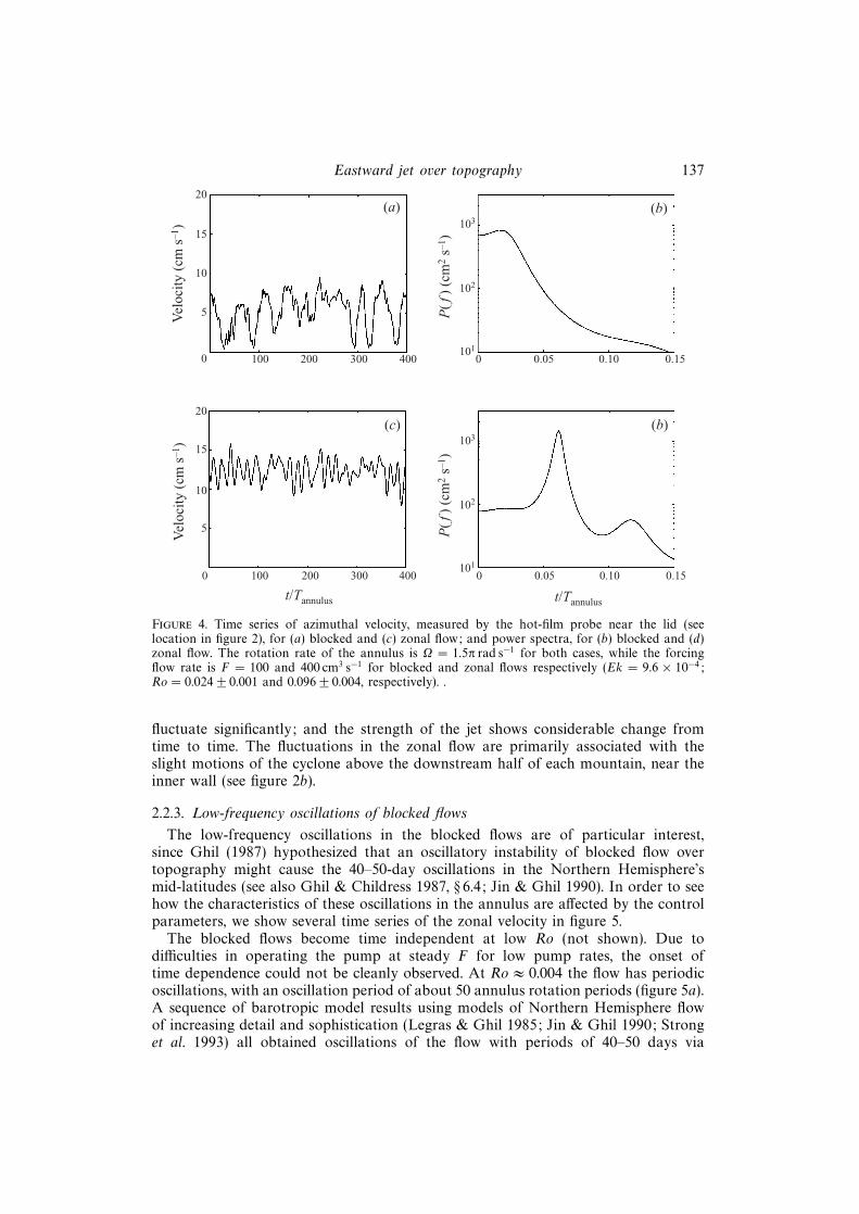
Blocked and zonal flows not only show distinct spatial patterns, but also exhibitqualitatively different temporal behaviour. An example appears in figure 4, showingtime series of azimuthal velocity for blocked and zonal flow. The blocked flow, shownin panel (a), has a small mean azimuthal velocity of 5.4 cm s−1, and exhibits large-amplitude, low-frequency fluctuations. By contrast, the zonal flow in panel (c) hasa much larger mean azimuthal velocity, of 12.0 cm s−1 in this case, but smaller andrapid fluctuations. The resonant velocity Ur for the rotation rate used in figure 4 is6.4 cm s−1.

Examination of the video and snapshots of the flows (not shown) reveals that thetime variability in the blocked flow manifests itself in several kinds of flow patternchanges: the strength and the orientation of the deep troughs on the downstreamflanks of the mountains (see figure 2a) undergo large variations with time; the shapeand the position of the small cut-off cyclones in the valleys, near the inner wall,


20

15

10

5

0 100 200 300 400

(a)

Vel

ocit

y (c

m s

–1) 103

102

1010 0.05 0.10 0.15

(b)

P(f

) (c

m2

s–1)

20

15

10

5

0 100 200 300 400

(c)

Vel

ocit

y (c

m s

–1)

t/Tannulus

103

102

1010 0.05 0.10 0.15

(b)P

(f)

(cm

2 s–1

)

t/Tannulus

Figure 4. Time series of azimuthal velocity, measured by the hot-film probe near the lid (seelocation in figure 2), for (a) blocked and (c) zonal flow; and power spectra, for (b) blocked and (d)zonal flow. The rotation rate of the annulus is Ω = 1.5π rad s−1 for both cases, while the forcingflow rate is F = 100 and 400 cm3 s−1 for blocked and zonal flows respectively (Ek = 9.6 × 10−4;Ro = 0.024± 0.001 and 0.096± 0.004, respectively). .

fluctuate significantly; and the strength of the jet shows considerable change fromtime to time. The fluctuations in the zonal flow are primarily associated with theslight motions of the cyclone above the downstream half of each mountain, near theinner wall (see figure 2b).

2.2.3. Low-frequency oscillations of blocked flows

The low-frequency oscillations in the blocked flows are of particular interest,since Ghil (1987) hypothesized that an oscillatory instability of blocked flow overtopography might cause the 40–50-day oscillations in the Northern Hemisphere’smid-latitudes (see also Ghil & Childress 1987, § 6.4; Jin & Ghil 1990). In order to seehow the characteristics of these oscillations in the annulus are affected by the controlparameters, we show several time series of the zonal velocity in figure 5.

The blocked flows become time independent at low Ro (not shown). Due todifficulties in operating the pump at steady F for low pump rates, the onset oftime dependence could not be cleanly observed. At Ro ≈ 0.004 the flow has periodicoscillations, with an oscillation period of about 50 annulus rotation periods (figure 5a).A sequence of barotropic model results using models of Northern Hemisphere flowof increasing detail and sophistication (Legras & Ghil 1985; Jin & Ghil 1990; Stronget al. 1993) all obtained oscillations of the flow with periods of 40–50 days via


4

2

0 100 200 300 400

0 100 200 300 400

0 100 200 300 400

0 100 200 300 400

4

2

4

2

4

2

(a) Ro = 4.2 × 10–3

(b) Ro = 8.4 × 10–3

(c) Ro = 2.1 × 10–2

(d) Ro = 4.2 × 10–2

t/Tannulus

Vel

ocit

y (c

m s

–1)

Figure 5. Velocity time series from blocked flow at low Ro. The Rossby numbers for each flow areindicated, with uncertainties ± 5%, and Ek = 4.8× 10−4 for all flows (Ω = 3π rad s−1). For the firsttime series (Ro = 0.0042), the period is 32 s = 48Tannulus. The pump rates for these flows are F = 25,50, 125, and 250 cm3 s−1. Time series for zonal flow at Ek = 4.8× 10−4 (not shown) are qualitativelysimilar to those seen in figure 4(c), which corresponds to zonal flow at Ek = 9.6× 10−4.

Hopf bifurcation of the blocked flow. These results suggest that the low-frequencyoscillations seen in figure 5(a) may also be due to a Hopf bifurcation, although thiscannot be determined directly from our experiments.

As the forcing is increased (figure 5b–d), the mean flow rate increases, and thefluctuations become more irregular and of higher amplitude. The power spectra ofthese time series are shown in figure 6. At Ro = 0.0042, there are pronounced peaksat 50 annulus periods and at the first harmonic of this frequency.

2.2.4. Regime diagram

Figure 7 shows the experiment’s phase diagram. For lower forcing F (lower Ro),the blocked state is stable; for higher forcing, the zonal state is stable. As the rotationrate Ω of the annulus is increased (lower Ek), stronger forcing is necessary to producea zonal flow. Due to the Ω−1/2 dependence of Ro, the pump flux F needed for zonalflow increases as Ω is increased (see (2.2) and (2.3)). This is consistent with theresonance argument. Faster rotation of the tank leads to a larger value of β, cf. (2.6),and consequently, a larger resonance velocity, cf. (2.5); this, in turn, requires a largerjet velocity to achieve super-resonance. On the other hand, when the jet is not strongenough, the flow tends to the subresonant, blocked state.

At intermediate Ro, either flow pattern can persist for fairly long time intervals.If the run is continued for long enough, however, the flow spontaneously switches


102

100

10–2

0 0.05 0.10 0.15

(a) Ro = 4.2 × 10–3

Pow

er (

cm2

s–1)

102

100

10–2

0 0.05 0.10 0.15

(c) Ro = 2.1 × 10–2

Pow

er (

cm2

s–1)

f /f annulus

102

100

10–2

0 0.05 0.10 0.15

(b) Ro = 8.4 × 10–3

102

100

10–2

0 0.05 0.10 0.15

(d ) Ro = 4.2 × 10–2

f /f annulus

Figure 6. Power spectra of the corresponding azimuthal velocity time series shown in figure 5, atΩ = 3π rad s−1 (Ek = 4.8 × 10−4) and different values of Ro. The spectra in this and subsequentfigures were obtained using the maximum-entropy method after data-adaptive pre-filtering bysingular-spectrum analysis (Dettinger et al. 1995).

between blocked and zonal flows. This is shown in figure 8(a), where the distinctsignatures of the two flow regimes can be seen. The transitions are clear cut, althoughthey take several annulus rotation periods to be completed (see figure 8b). Suchtransitions occur at irregular intervals and do not appear predictable.

The time the flow spends in one regime before it switches to the other is quitevariable, but is much longer than the oscillation periods of either the zonal orblocked flows: each flow regime usually persists for at least a few hundred annulusrotations, and sometimes thousands, before it switches to the other regime. Thealternation between fairly long stays in either regime, on the one hand, and fairlyrapid transitions between regimes, on the other, is very similar to that seen in thebarotropic model of Legras & Ghil (1985). Weeks et al. (1997) described how thepercentage of time spent in the blocked regime decreases with Rossby number (seefigure 4 there). They also discussed how this result compares with similar propertiesof observed atmospheric flows (Dole & Gordon 1983) and of flows in a barotropicmodel on the sphere (Legras & Ghil 1985).

We have carried out selected experiments at higher rotation rates, up to Ω =6π rad s−1, although not in the detail necessary to extend our phase diagrams (figure 7).Blocked and zonal flow patterns are both present at these higher rotation rates, aswell as the spontaneous transitions between them.


0.0010

0.0005

0.02 0.04 0.06 0.08 0.10

Rossby number

Ekm

an n

umbe

r

4(a) 4(c)

5(b) 5(c)

5(a)

5(d)

2(b)

Blocked

Intermittent

Zonal

Figure 7. Phase diagram showing regions of differing flow patterns in the experiment, as a functionof Ro and Ek. In each of the two regions labelled ‘Blocked’ and ‘Zonal’, the resulting flows arestable, resemble the pattern associated with the respective label, and occur from any initial state.In the middle region between the two that is labelled ‘Intermittent’, the flow pattern switchesspontaneously between the blocked and zonal flows. The black dots at the boundaries of this regionare derived from experimental runs at constant Ek by using the highest and lowest values of Rowhere intermittent behaviour was found (see also figure 4 in Weeks et al. 1997). The locations ofexperimental runs used for figures 2, 4, 5 and 8 are indicated by asterisks.

3. Numerical investigation3.1. Model formulation

3.1.1. Governing equation

Our model is governed by the quasi-geostrophic barotropic potential-vorticity equa-tion, since the flow in the rotating annulus is predominantly two-dimensional andnearly geostrophic, due to the rapid rotation of the annulus. Including vorticity forc-ing, Ekman friction and eddy viscosity, the dimensional form of the equation is (Ghil& Childress 1987; Pedlosky 1987; Marcus & Lee 1998),

∂

∂t(∇2ψ) + J(ψ,∇2ψ) +

fs

H

∂ψ

∂x+f

HJ(ψ, h) = − (2AVf)1/2

H∇2(ψ − ψ∗) + ν∇4(ψ − ψ∗).

(3.1)

On the left-hand side, J is the Jacobian operator, ψ = ψ(x, y, t) is the streamfunction,H is the mean depth of the fluid, f = 2Ω is the Coriolis parameter, s is the tank’sbottom slope, and h = h(x, y) is the height of the topography measured from theunderlying sloping bottom. We follow Lorenz (1963) in neglecting the curvature ofthe annular gap in the tank, so that x corresponds to rθ and y to r; y, however, pointstoward the axis of rotation or ‘poleward’, in the customary atmospheric analogy.

The right-hand side of (3.1) includes the forcing, Ekman friction and eddy viscosity;ψ∗ = ψ∗(x, y) is the streamfunction of the external forcing field, which produces theeastward jet and whose exact form will be derived further below (see (3.7) and (3.8)).The vertical component AV of the turbulent viscosity coefficient in the frictionalboundary layers is taken to be the same at the top and bottom (Charney & DeVore


5

4

3

2

1

0

0 2000 4000 6000

Zonal Zonal

(a) Blocked Blocked

Vel

ocit

y (

cm s

–1)

5

4

3

2

1

03000 3250 3500

(b)Vel

ocit

y (

cm s

–1)

t /Tannulus

Figure 8. Spontaneous transitions between the two flow states, as seen in the azimuthal velocitysignal. The parameters Ro = 0.0475 ± 0.001 and Ek = 4.8 × 10−4 are held fixed (rotation rateΩ = 3π rad s−1 and pump flux F = 280 cm3 s−1). Part (b) shows an expanded view of one of thetransitions from (a).

1979; Gill 1982; Pedlosky 1987), and ν is the eddy coefficient of lateral viscositythat simulates the effect of the subgrid-scale motions on the flow (Smagorinsky 1963;Kraichnan 1976).

To non-dimensionalize (3.1) we introduce the scaled variables,

x = arLx′, y = Ly′, t = art

′/f,h = Hh′, ψ = L2fψ′, ψ∗ = L2fψ′∗,ν = L2fν ′,

(3.2)

where L is chosen as the length scale, 1/f as the time scale, and Lf as the velocityscale, while ar is the aspect ratio of the channel. This yields the non-dimensionalequation, with the primes dropped for convenience,

∂

∂t(∇2ψ) + J(ψ,∇2ψ + hm) + β

∂ψ

∂x= −arκ∇2(ψ − ψ∗) + arν∇4(ψ − ψ∗). (3.3)

The non-dimensional Laplacian operator in (3.3) is defined as

∇2ψ ≡(

∂2

a2r ∂x

2+

∂2

∂y2

)ψ, (3.4)

and the two non-dimensional parameters on the right-hand side are defined as

β =Ls

H, κ =

(2AVf)1/2

fH. (3.5)


Formally, the κ defined in (3.5) is related to the Ekman number defined for theexperiment in § 2 by κ2 = Ek. The actual value of κ, however, is determined by theturbulent viscosity AV in the boundary layer, which is a function of the flow, ratherthan by the kinematic viscosity ν, which is intrinsic to the fluid (Gill 1982; Pedlosky1987). Therefore, κ can only be determined empirically in our numerical calculations,and we use κ-values from 0.001 to 0.01, based on qualitative similarity of the flowdynamics with the tank experiments.

As the vorticity forcing ψ∗ does not change with time, once ν, ψ∗ = ψ∗(x, y), andh = h(x, y) are specified, the dynamics described by (3.3) is completely determined bythe two parameters β and κ and the initial streamfunction field ψ(x, y, 0).

3.1.2. Numerical formulation

The model equation (3.3) is solved numerically in a straight and periodic channel,neglecting the curvature of the tank, with a dimensionless width of π between thetwo lateral boundaries and spatial period of arπ in the zonal direction (Lorenz 1963;Charney & DeVore 1979; Ghil & Childress 1987, §§ 5.2 and 6.3). Free-slip boundaryconditions are imposed on the two sidewalls.

We use a pseudospectral method with de-aliasing (e.g. Orszag 1971) for spatialdiscretization, and a second-order predictor–corrector scheme for time integration(Lorenz 1963). There are 32 spectral modes in each spatial direction, but the nonlinearterms are computed using 64× 64 modes before dealiasing. Different time-step sizesand numbers of spatial modes, as well as other time integration schemes, have beentested to ensure the accuracy and physical realism of the numerical results.

The model parameters are chosen to match the laboratory settings. The aspectratio ar is chosen as the ratio of the mid-channel perimeter to the wall-to-wall widthof the annulus, which yields ar = 5π/3. The length scale L is the same order as theazimuthal extent of either mountain, taken to be 28 cm; H = 18.7 cm is the meandepth of the water in the tank. Hence we have, from (3.5),

β =Ls

H=

28× 0.1

18.7= 0.15. (3.6)

As mentioned in the previous subsection, the value of the Ekman friction coefficientκ is chosen so that the model dynamics is similar to that in the experiment, since theturbulent viscosity AV cannot be determined directly from the experiment. Our rangeof κ from 0.001 to 0.01 corresponds approximately to a reasonable range of AV from0.001 to 0.1 cm2 s−1. The value of the eddy viscosity ν is determined by trial and error(McWilliams et al. 1981), and we found that 10−6 < ν < 10−4 is a reasonable range.

The topography and forcing in the numerical model are like those in the tank.Two symmetric Gaussian ridges are specified, as in (2.1), and we tested two non-dimensional heights of the mountains: h0 = 0.1, which is about the same heightas the experimental mountains, and h0 = 0.15. The forcing by the fluid pumpedthrough the two rings of holes in the tank is simulated in the barotropic model asvorticity forcing, based on the quasi-geostrophic relation between vertical velocity inthe bottom boundary layer and the induced free-fluid vorticity (see Pedlosky 1987,figure 4.5.1 and equation (4.5.39)). We use this Ekman pumping relation in the form

w∗(x, y) =

(AV

2f

)1/2

∇2ψ∗(x, y), (3.7)

where w∗ is the forced vertical velocity through the holes, and ψ∗(x, y) is the forcingvorticity.


Inner ring

Outer ring

–A A

Vorticity

y

p

Figure 9. The cross-channel profile of the forcing vorticity in the numerical model. The width of thechannel is π, while the simulated outer ring is located at y1 = π/4 and the inner ring at y2 = 3π/4.The profile is given by (3.8) and the amplitude A is arbitrary.

Assuming w∗ has a narrow Gaussian profile in the radial direction over either ring,we model the vorticity forcing as

∇2ψ∗(x, y) = A[exp (−(y − y2)2/y2

0)− (7/13) exp (−(y − y1)2/y2

0)]; (3.8)

here A is the forcing amplitude, and y0 = π/32 is the e-folding width of the narroww∗ profile in the radial direction, with y1 = π/4 and y2 = 3π/4 being the positionof the outer ring and inner ring, respectively. The value of y0 is chosen to be smallenough to simulate the relative narrowness of the two rings in the annulus, while stilllarge enough to have the forcing profile resolved by the numerical grid. The factor7/13 comes from the fact that the averaged w∗ along the outer ring is weaker thanthe inner ring because the outer ring has a longer perimeter, while the total water fluxis the same through both. The vorticity forcing profile so obtained across the channelis shown in figure 9, with positive (negative) vorticity in the inner (outer) ring.

A Rossby number Ro of the forcing can be defined – independent of the flow details,as was done for the experiment – by integrating (3.8) over y to find the velocity profile,assuming axisymmetric flow and imposing a zero-slip boundary condition at y = 0.The exact form is complicated, but at y = π/2 (the axis of the channel) the solutionis approximately

U = 12y0π

1/2A, (3.9)

with y0 = π/32 as discussed above. Due to the choice of non-dimensional units (see(3.2)), Ro = U; for our value of y0 this simplifies to Ro ≈ 0.017A.

3.2. Simulation results

3.2.1. Blocked and zonal flows

The numerical model reproduces the blocked and zonal flows seen in the experi-ments, over a wide range of parameters. Figure 10 shows typical blocked and zonalflow patterns, projected from the model’s straight-channel geometry to annular geom-


(a) (b)

Figure 10. The time-averaged streamfunction field of the two types of flow seen in the numericalmodel, (a) blocked and (b) zonal. The parameters for the two cases are the same, with A = 2.0,h0 = 0.15, κ = 0.01, and ν = 5× 10−5. The straight channel in the model is projected to the annularshape shown in the figure, with the shaded areas indicating the coverage of the mountains. Contourintervals: (a) 0.0125; (b) 0.025. The squares show the position of the simulated velocity probe.Compare these streamfunctions with those observed in the experiments (figure 2).

0.25

0.20

0.15

0.10

0.05200 300 400 500 600 700

Zonal

Blocked

T/Trotation

Zon

al v

eloc

ity

Figure 11. The non-dimensional zonal-velocity time series of the two flows in figure 10, measuredat the position shown by the filled square, the same position as the hot-film probes in the tank. Theazimuthal velocity of 0.20 is equivalent to a dimensional velocity of 70 cm s−1 at a tank rotationrate of Ω = 2π rad s−1.

etry; this projection facilitates comparison with the laboratory experiments. Figure 11shows the azimuthal velocity signals for the blocked and zonal flows.

The major features of the simulated blocked and zonal flows are qualitativelysimilar to their experimental counterparts. Both simulation (figure 10) and experiment(figure 2) show that the zonal flow has a strong jet with little meandering, andthe associated cyclones near the inner wall lie over the downstream half of thetopography. The zonal flows have small-amplitude, higher-frequency fluctuations inthe jet velocity signal. Blocked flow in both simulation and experiment has a weak jetwith pronounced meandering and two deep troughs on the downstream flank of themountains. The blocked flows also have large-amplitude, low-frequency oscillationsin the jet velocity, in both the experiment and the simulation (cf. figure 4a and


0.15

0.10

0.05

0 1 2 3 4

(a) h0 = 0.10, j = 0.004

Mea

n zo

nal v

eloc

ity

0.15

0.10

0.05

0 1 2 3 4

(c) h0 = 0.10, j = 0.010

Mea

n zo

nal v

eloc

ity

Forcing amplitude, A

0.15

0.10

0.05

0 1 2 3 4

(b) h0 = 0.15, j = 0.004

0.15

0.10

0.05

0 1 2 3 4

(d ) h0 = 0.15, j = 0.010

Forcing amplitude, A

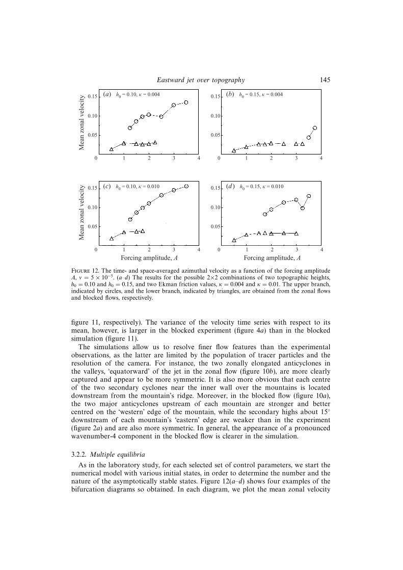
Figure 12. The time- and space-averaged azimuthal velocity as a function of the forcing amplitudeA, ν = 5 × 10−5. (a–d) The results for the possible 2×2 combinations of two topographic heights,h0 = 0.10 and h0 = 0.15, and two Ekman friction values, κ = 0.004 and κ = 0.01. The upper branch,indicated by circles, and the lower branch, indicated by triangles, are obtained from the zonal flowsand blocked flows, respectively.

figure 11, respectively). The variance of the velocity time series with respect to itsmean, however, is larger in the blocked experiment (figure 4a) than in the blockedsimulation (figure 11).

The simulations allow us to resolve finer flow features than the experimentalobservations, as the latter are limited by the population of tracer particles and theresolution of the camera. For instance, the two zonally elongated anticyclones inthe valleys, ‘equatorward’ of the jet in the zonal flow (figure 10b), are more clearlycaptured and appear to be more symmetric. It is also more obvious that each centreof the two secondary cyclones near the inner wall over the mountains is locateddownstream from the mountain’s ridge. Moreover, in the blocked flow (figure 10a),the two major anticyclones upstream of each mountain are stronger and bettercentred on the ‘western’ edge of the mountain, while the secondary highs about 15downstream of each mountain’s ‘eastern’ edge are weaker than in the experiment(figure 2a) and are also more symmetric. In general, the appearance of a pronouncedwavenumber-4 component in the blocked flow is clearer in the simulation.

3.2.2. Multiple equilibria

As in the laboratory study, for each selected set of control parameters, we start thenumerical model with various initial states, in order to determine the number and thenature of the asymptotically stable states. Figure 12(a–d) shows four examples of thebifurcation diagrams so obtained. In each diagram, we plot the mean zonal velocity


0.1

0 100 200 300 400 500 600 700

2.50

2.00

1.75

1.50

1.00

0.50

Time (rotations)

(a)

(b)

10–4

10–6

0 0.1 0.2 0.3 0.4

Frequency (rotation–1)

2.50

2.00

1.75

1.50

1.000.50

ME

M p

ower

Zon

al v

eloc

ity

Figure 13. (a) Time series of the blocked-flow azimuthal velocity at the location of the simulatedprobe (see figure 10a), for various forcing amplitudes A, as labelled next to each curve. (b) Powerspectra of the corresponding time series in (a), estimated using the maximum-entropy method. Otherparameters: h0 = 0.15, κ = 0.006, and ν = 5 × 10−5. All the curves in each panel are displayed onthe same scale but displaced vertically to avoid overlapping.

of each stationary stable state reached by our model runs, averaged over the wholechannel, as a function of the forcing amplitude A.

Both types of flow are present in all four cases, with zonal flows having a largervelocity than the blocked flows in each case. The mean zonal velocity of the zonal flowsincreases with the forcing amplitude, except for the minor ‘dips’ in figures 12(a) and12(d), whereas in blocked flows the mean azimuthal velocity stays fairly flat after someinitial increase while the forcing is still weak. In addition, zonal flows tend to exist overthe higher range of the forcing, while blocked flows tend to be confined to the lowerrange. Both the maximal height of the topography h0 and the Ekman friction κ havea substantial influence on the stability of either flow. By increasing h0 or decreasing κ,blocked flow remains stable up to higher values of the forcing A, while by decreasingh0 or increasing κ, the stability of zonal flow at lower values of A is increased.

Furthermore, except in figure 12(b), there is a sizable range in the forcing amplitudein which stable zonal and blocked flows coexist. This indicates that the asymptotic


104

102

100

10–2

10–4

0 0.1 0.2 0.3 0.4

0.004

0.006

j =0.010

(a)

101

100

10–1

10–2

10–4

0 0.1 0.2 0.3 0.4

0.004

0.006

j =0.010

(b)

ME

M p

ower


10–3

ME

M p

ower

Figure 14. Maximum-entropy spectra of the zonal-velocity time series of the blocked flows fortwo mountain heights, (a) h0 = 0.10 and (b) h0 = 0.15, and various values of Ekman friction κ.Forcing amplitude A = 1.75 in both cases and ν = 5× 10−5. The curves are displayed on the samelogarithmic scale but displaced vertically to avoid overlapping.

state reached by the flow does depend on the initial state, and multiple equilibria doexist for a wide range of parameter values (cf. figure 12a, c, d).

The pseudo-arclength continuation code described in Appendix B of Tian (1999)was applied to a number of preliminary versions of the model. It gave in all casesS-shaped bifurcation curves for the jet’s intensity that resemble figure 6.5 of Ghil &Childress (1987), with zonal flows on the upper branch and blocked flows on thelower branch. This suggests that for the model version analysed in detail here, themultiple equilibria are due to back-to-back saddle–node bifurcations.

3.2.3. Low-frequency oscillations of blocked flows

We have examined the effect of forcing, topographic height, and Ekman friction onthe blocked-flow low-frequency oscillations. Figure 13 shows velocity time series and


304 308

310 312

315 319

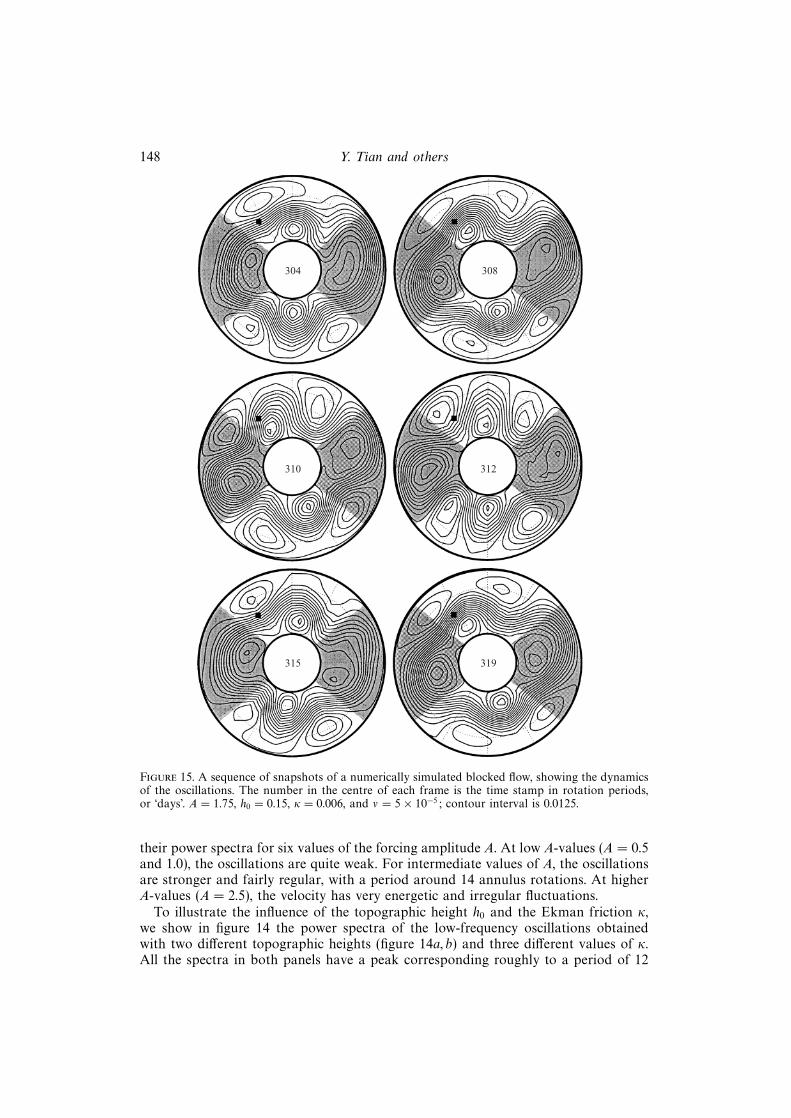
Figure 15. A sequence of snapshots of a numerically simulated blocked flow, showing the dynamicsof the oscillations. The number in the centre of each frame is the time stamp in rotation periods,or ‘days’. A = 1.75, h0 = 0.15, κ = 0.006, and ν = 5× 10−5; contour interval is 0.0125.

their power spectra for six values of the forcing amplitude A. At low A-values (A = 0.5and 1.0), the oscillations are quite weak. For intermediate values of A, the oscillationsare stronger and fairly regular, with a period around 14 annulus rotations. At higherA-values (A = 2.5), the velocity has very energetic and irregular fluctuations.

To illustrate the influence of the topographic height h0 and the Ekman friction κ,we show in figure 14 the power spectra of the low-frequency oscillations obtainedwith two different topographic heights (figure 14a, b) and three different values of κ.All the spectra in both panels have a peak corresponding roughly to a period of 12


0.25

0.20

0.15

0.10

0.05

300 316 324 332 340308

Time (rotation)

Zon

al v

eloc

ity

304

308

310

312

315

319

0

Figure 16. The azimuthal velocity measured at the probe position (square in figure 10a), includingthe time interval over which the oscillations are shown in figure 15. The six time stamps on thecurve correspond to the six frames shown in figure 15.

annulus rotations. However, the spectra in figure 14(a), for lower mountains, havea sharper peak near this period than those in figure 14(b); thus the oscillations inthe lower-mountain case tend to be more regular. Increasing the Ekman friction κsharpens the peaks in either case, but does not change their location very much.

The blocked flows’ oscillatory instability and its parameter dependence have beenstudied by Jin & Ghil (1990) in an analytic, weakly nonlinear model and by Stronget al. (1993, 1995) and Keppenne et al. (2000) in numerical models. The oscillations’main mechanism is the topographic modulation of the interaction between the sta-tionary wave, whose ridge lies upstream of the topographic ridge, and the zonal flow.Oscillations in the wave’s amplitude and the zonal position of its ridge are accom-panied by oscillations in the torque that wave exerts on the mountains; the latteroscillations are counterbalanced by oscillations of the opposite sign in the torqueexerted by the zonal flow’s varying intensity. The sharper peaks obtained at the mainperiod in the experiment for lower topography and stronger Ekman dissipation areconsistent with the nonlinear effects decreasing with smaller h0 and larger κ.

To verify the main features of the blocked-flow oscillations – as described in theabove-cited earlier work – we show a sequence of snapshots of the streamfunctionfield in figure 15. The six frames in the sequence correspond to slightly more thanone cycle, with an approximate 90 phase difference between two consecutive frames.The exact phase of each frame is shown on the velocity signal for the same numericalrun, displayed in figure 16.

The low-frequency oscillations in the strength and length of the jet are accompa-nied by changes in the shape, intensity and azimuthal position of the cyclonic andanticyclonic vortices, as well as by exchanges of kinetic energy between the jet andthe vortices. They have the character of relaxation oscillations, already attributed byNamias (1950) to the atmospheric index cycle: the kinetic energy of the jet growsslowly (through roughly 7 rotations) and is discharged rapidly (over about 4 rotations)into the vortices (see figures 15 and 16). These oscillations are close to periodic, butnot perfectly regular.

The flow fields in figure 15 are dominated by components of zonal wavenumber-2and their harmonics of wavenumber-4, which confirms the controlling role of thetopography. On the other hand, the flow fields are not perfectly symmetric with


0.02

0.03

0.02

0.020.03

0.03

0.02

0.02

0.02

0.03

Figure 17. Variance of the streamfunction field of the blocked flow shown in figure 15. The dashedlines indicate the edges of the mountains. Contour interval: 0.005, with regions larger than 0.03shaded.

respect to a shift by arπ/2, the half-length of the channel, in the zonal direction;this implies that odd wave components are present, due to their nonlinear interactionwith the topography (Tian 1997).

To see the spatial distribution of the oscillation’s variability, we calculated thevariance of the streamfunction of the flow shown in figure 15 over a long timeinterval. The result is displayed in figure 17, with the areas of largest variabilityshaded. These areas are located roughly along the path of the jet, especially where itruns around the deep troughs over the mountains, and over the secondary cyclonesbetween the mountains. The largest area of strong variability covers the downstreamflank of each deep trough; a smaller area with the same amplitude of variability isfound on the upstream side of each secondary cyclone. The centres of the troughsand cyclones, however, exhibit very little variability, and so do the regions near thetwo sidewalls.

3.2.4. Oscillations in the zonal flows

The small–amplitude fluctuations in the zonal flows (see figure 11) were alsostudied in the numerical model. Figure 18 shows the azimuthal velocity time seriesand the corresponding power spectra for six different values of the forcing amplitude.The amplitude of the oscillations (see panel a) increases as the forcing increases.The spectra (see panel b) reveal that each oscillation has a dominant frequency,accompanied by several harmonics or subharmonics. These secondary frequenciesare regularly distributed and occupy much of the range of 1 to 10 rotation periods,with various amplitudes relative to the dominant peak. No systematic change in thelocation and amplitude of the dominant frequency, nor in the relative amplitude ofthe secondary frequencies can be observed as the forcing increases. The frequenciesare all, however, higher than those that characterize the blocked-flow oscillations.

Inspection of the flow fields (not shown) indicates that these oscillations in the jetvelocity are mainly induced by the slight libration movement of the two secondarycyclones. Located on the inner-wall side of the jet and close to the wall, these cyclonesappear to be driven by the shear between the jet and the wall. They move back and


0.2

0.1

(a)

400 500 600 700

Time (rotations)

3.50

3.00

2.50

2.00

1.75

1.50

(b)

3.50

3.00

2.50

2.00

1.75

1.50

0 0.2 0.4 0.6 0.8


10–4

10–6

ME

M p

ower

Zon

al v

eloc

ity

Figure 18. (a) Time series and (b) maximum-entropy spectra of the azimuthal velocity time seriesmeasured at the probe position in the zonal flows. The numbers on each curve are the forcingamplitude A; h0 = 0.10, κ = 0.01, and ν = 5 × 10−5. The curves are displaced vertically to avoidoverlapping.

forth slightly – with some change in intensity but without significant effect on theshape of the jet – over the downstream flank of the two mountains.

4. Summary and discussion4.1. Comparison between laboratory and numerical results

In laboratory experiments on a barotropic rotating annulus with two symmetric,Gaussian-shaped mountains as the bottom topography (figure 1), two distinct flowpatterns were obtained. One of them resembles atmospheric high-index or zonalflows, the other low-index or blocked flows in the atmosphere (see figure 2). Thephase relations between the main flow features and the topography, as well as thecorresponding azimuthal velocity of the jet, show that topographic resonance affectsthe flows: the zonal flows appear super-resonant, while the blocked flows appear to besubresonant. The jet velocity of zonal flow is higher than the critical velocity for linear


resonance of Rossby waves with the topography, while the jet velocity of blocked flowis lower than this resonant velocity (figure 4). The important role of the topographyis also seen from the dominance of zonal wavenumber-2 in both zonal and blockedflows, and the flow patterns’ nearly fixed position relative to the mountains.

Blocked flows are stable at low Ro and Ek. Between the two regimes in parameterspace where either flow is stable lies a region where the flow switches intermittentlyfrom one flow pattern to the other (see figure 7).

Essentially the same flow patterns, zonal and blocked, were obtained in a numericalmodel designed to simulate the flow in the rotating annulus. However, quantitativecomparison is not possible because the numerical model’s parameters A and κ cannotbe determined directly from the experiment. Further, the simulation neglects sidewalland curvature effects. Nevertheless, the two types of flow regimes in the model,zonal and blocked, have much the same spatial and temporal characteristics as theircounterparts in the experiment. These common characteristics include the shape andposition of the cyclonic and anticyclonic vortices in the flow (compare figure 2 andfigure 10), the strength and configuration of the jet, the large-amplitude low-frequencyoscillations associated with the blocked flows, and the small-amplitude fluctuationsassociated with the zonal flows (compare figure 4 and figure 11).

In the numerical model, multiple equilibria exist for a wide range of parameters(figure 12). Higher mountains lead to stronger nonlinear interactions between themountains and the flow and, when the flow is stabilized by sufficient Ekman friction,there is a rather large region in which the two flow patterns coexist as stable equilibria(see figure 12d). This is in contrast to the laboratory experiments, where no multipleequilibria were observed. Instead, at moderate Ro both flows in the rotating annulusare metastable, and spontaneous transitions between the two take place abruptly andat irregular intervals.

Two-way spontaneous transitions between the zonal and blocked flows have notbeen found in the numerical model. Since there is a certain amount of noise inthe tank’s forcing, O(1 cm3 s−1), we tried adding white noise to the forcing in thenumerical model; even when the noise was fairly strong, however, no transitions wereobserved. Furthermore, as the Ekman friction is a function of the flow instead of thefluid, we tested various parameterization schemes (e.g. Gill 1982, Chap. 9; Stull 1988,Chap. 6) to relate the friction with the properties of the flow, such as the velocityor kinetic energy. Various schemes had different effects on the dynamics of the flow,but did not result in spontaneous transitions. A change in the forcing profile and adifferent formulation of the eddy viscosity term (Treguier & McWilliams 1990; Ghil& Paldor 1994) did not induce the transitions either. In a similar numerical modelbut with a different jet profile and simplified mountains (Tian 1997), no transitionswere observed in spite of the existence of similar blocked and zonal flow states.

One possible explanation is that three-dimensional effects in the laboratory flows,not captured by our purely two-dimensional models, may have played an importantrole during the transition. We have observed during the transition that the large-scale coherent structure of either flow pattern, zonal or blocked, first breaks intosmaller-scale, turbulent flows, and then reorganizes itself into the other metastableflow pattern. Moreover, zonal flows have several times as much kinetic energy as theblocked ones and, during the short transition interval to blocked flow, a considerableamount of kinetic energy must be dissipated. Small-scale three-dimensional turbulentflow features would help dissipate this energy.

We tried to test this hypothesis by examining the velocity records from the top andbottom hot-film probes, for indications of loss of correlation during the transitions.


The rapidity of the transitions, however, makes it difficult to determine whether thevelocities at the tank’s top and bottom become uncorrelated during a transition.Further studies are needed on the detailed physical processes that operate during thetransitions. This will require a model with three-dimensional dynamics and possiblyhigher horizontal resolution.

The azimuthal velocity in the numerical model’s blocked flows is typically about35 cm s−1, which is larger than that obtained for similar conditions in the experiments;the latter is usually less than 20 cm s−1. We speculate that the disagreement is dueto two reasons. One is that we used a continuous band of forcing vorticity alongthe channel in the numerical model, rather than 120 small discrete holes as in theexperiment. The former is much more efficient in forcing the jet. The other is theabsence of friction from the two sidewalls in the numerical model, in which weimposed free-slip boundary conditions. This friction, though less effective than theEkman friction in the top and bottom layers, may damp the jet velocity and lowerthe frequency of the oscillations. The presence of the lateral boundaries might alsoplay a role in the three-dimensional flow effects mentioned in the previous paragraph.

4.2. Connections to the atmosphere

The two types of flows we obtained in the tank and in the model are qualitativelysimilar to high- and low-index, or zonal and blocked flows in the atmosphere. Still,the atmosphere’s large-scale persistent flow patterns are clearly more complicated.In spite of the complexity of ever-changing weather patterns and the shortness ofinstrumental records, observational studies have determined that multiple regimes canbe identified (Cheng & Wallace 1993; Kimoto & Ghil 1993a, b; Michelangeli, Vautard& Legras 1995). More precise relationships between the two types of flow found here,experimentally and numerically, and the flow regimes in the Northern Hemisphere’satmosphere remain to be determined. This task is rendered more difficult by the factthat – in spite of recent progress in this direction – there is still no consensus on theexact number and flow patterns of the Northern Hemisphere’s flow regimes.

Cheng & Wallace (1993), Kimoto & Ghil (1993a), Smyth, Ide & Ghil (1999), andCorti, Molteni & Palmer (1999) all essentially find two regimes, zonal and blocked,in each one of the Pacific/North-American and Atlantic–European sectors of thehemisphere. But Kimoto & Ghil (1993b), Michelangeli et al. (1995) and Robertson &Ghil (1999), among others, each find slightly larger numbers of regimes in one or theother of the sectors, or both. The latter represent a finer subdivision of the two regimes,zonal and blocked, obtained by the ‘conservative’ or ‘parsimonious’ classification of theformer set of authors. This subdivision in the ‘richer classifications’ might correspondto an identification as separate regimes of slow phases of an oscillation about blockedflow like the one described here in some detail. It might correspond, on the otherhand, to the existence of regimes that have distinct physical origins but, being moresparsely populated (at least over the last half-century of instrumental upper-air data),get lumped into a single regime by the more conservative classification methods.

Although our original motivation for these investigations arose from the multi-ple regimes and intraseasonal oscillations that contribute to the atmosphere’s low-frequency variability, we do not expect to obtain straightforward answers to thequestions raised by the real atmosphere from the results obtained in our idealizedrotating annulus and numerical models. Nevertheless, explorations like those reportedhere do provide insight into the fundamental dynamics, and suggest guidelines foranalysis of the atmospheric observations.

Oscillations are present in zonal and blocked flows in both the annulus and the


atmosphere. In the atmosphere, the oscillations about zonal flows arise mainly frombaroclinic instability, not present in our barotropic annulus and model. The low-frequency oscillations about the blocked flows in our study, however, are more likelyto have common features with the observed ones (see Ghil & Robertson 2000 fora recent review of work on intraseasonal oscillations in the Northern Hemisphereextratropics). The description and energy diagnostics of the oscillations here can thushelp prove or disprove a topographic origin for the atmospheric oscillations.

We thank P. Billant, M. Kimoto, L. Panetta, B. Plapp, and D. J. Tritton (deceased;see H. L. Swinney & P. A. Davies, Phys. Today vol. 52 (1999), p. 82) for helpfuldiscussions. Constructive comments from five anonymous reviewers greatly improvedthe presentation. The laboratory experiments (E. R. W., J. S. U., C. N. B., H. L. S.)were supported by the Office of Naval Research and the numerical studies weresupported by NASA grant NAG 5–9294 (K. I. and Y. T.) and by an NSF SpecialCreativity Award (M. G.). M. G. furthermore thanks his hosts at the Ecole NormaleSuperieure in Paris for their hospitality during the sabbatical that helped completethis work. This is publication number 5483 of UCLA’s Institute of Geophysics andPlanetary Physics.

REFERENCES

Anderson, J. R. & Rosen, R. D. 1983 The latitude-height structure of 40–50 day variations inatmospheric angular momentum. J. Atmos. Sci. 40, 1584–1591.

Bernardet, P., Butet, A., Deque, M., Ghil, M. & Pfeffer, R. L. 1990 Low-frequency oscillationsin a rotating annulus with topography. J. Atmos. Sci. 47, 3023–3043.

Bolin, B. 1950 On the influence of the earth’s orography on the general character of the westlies.Tellus 2, 184–195.

Carnevale, G. F., Kloosterziel, R. C. & Heijst, G. J. F. van 1991 Propagation of barotropicvortices over topography in a rotating tank. J. Fluid Mech. 233, 119–139.

Charney, J. G. & DeVore, J. G. 1979 Multiple flow equilibria in the atmosphere and blocking. J.Atmos. Sci. 36, 1205–1216.

Charney, J. G. & Eliassen, A. 1949 A numerical method for predicting the perturbations of themiddle latitude westerlies. Tellus 1, 38–54.

Charney, J. G., Shukla, J. & Mo, K. C. 1981 Comparison of a barotropic blocking theory withobservation. J. Atmos. Sci. 38, 762–779.

Charney, J. G. & Straus, D. M. 1980 Form-drag instability, multiple equilibria and propagatingplanetary waves in baroclinic, orographically forced, planetary wave systems. J. Atmos. Sci. 37,1157–1176.

Cheng, X. & Wallace, J. M. 1993 Cluster analysis of the Northern Hemisphere wintertime 500–hpaheight field spatial patterns. J. Atmos. Sci. 50, 2674–2696.

Corti, S., Molteni, F. & Palmer, T. N. 1999 Signature of recent climate change in frequencies ofnatural atmospheric circulation regimes. Nature 398, 799–802.

Dettinger, M. D., Ghil, M., Strong, C. M., Weibel, W. & Yiou, P. 1995 Software expeditessingular–spectrum analysis of noisy time series. EOS, Trans. AGU 76, 14–21 (see alsohttp://www.atmos.ucla.edu/tcd/).

Dickey, J. O., Ghil, M. & Marcus, S. L. 1991 Extratropical aspects of the 40–50 day oscillationin length-of-day and atmospheric angular momentum. J. Geophys. Res. 96, 22643–22658.

Dole, R. M. & Gordon, N. D. 1983 Persistent anomalies of the extratropical Northern Hemispherewinter time circulation: Geographical distribution and regional persistence characteristics.Mon. Wea. Rev. 111, 1567–86.

Dowling, T. E. & Ingersoll, A. P. 1989 Jupiter’s Great Red Spot as a shallow water system. J.Atmos. Sci. 46, 3256–3278.

Egger, J. 1978 Dynamics of blocking highs. J. Atmos. Sci. 35, 1788–1801.

Ghil, M. 1987 Dynamics, statistics, and predictability of planetary flow regimes. In Irreversible


Phenomena and Dynamical Systems Analysis in the Geosciences (ed. C. Nicolis & G. Nicolis),pp. 241–283. Reidel.

Ghil, M. & Childress, S. 1987 Topics in Geophysical Fluid Dynamics Atmospheric Dynamics,Dynamo Theory, and Climate Dynamics. Springer.

Ghil, M. & Mo, K. 1991 Intraseasonal oscillations in the global atmosphere. Part I. NorthernHemisphere and tropics. J. Atmos. Sci. 48, 752–779.

Ghil, M. & Paldor, N. 1994 A model equation for nonlinear wavelength selection and amplitudeevolution of frontal waves. J. Nonlin. Sci. 4, 471–96.

Ghil, M. & Robertson, A. W. 2000 Solving problems with GCMs: General circulation models andtheir role in the climate modeling hierarchy. In General Circulation Model Development: Past,Present, and Future (ed. D. Randall), pp. 285–325. Academic.

Gill, A. E. 1982 Atmosphere–Ocean Dynamics. Academic.

Greenspan, H. P. 1968 The Theory of Rotating Fluids. Cambridge.

Hart, J. E. 1979 Barotropic quasi-geostrophic flow over anisotropic mountains. J. Atmos. Sci. 36,1736–1746.

Held, I. M. 1983 Stationary and quasi-stationary eddies in the extratropical troposphere: theory.In Large-Scale Dynamical Processes in the Atmosphere (ed. B. J. Hoskins & R. P. Pearce), pp.127–169. Academic.

Holloway, G. 1992 Representing topographic stress for large-scale ocean models. J. Phys. Oceanogr.22, 1033–1046.

Jin, F.-F. & Ghil, M. 1990 Intraseasonal oscillations in the extratropics: Hopf bifurcation andtopographic instabilities. J. Atmos. Sci. 47, 3007–3022.

Jonas, P. R. 1981 Laboratory observations of the effects of topography on baroclinic instability. Q.J. R. Met. Soc. 107, 775–792.

Keppenne, C. L. & Ingersoll, A. P. 1995 High-frequency orographically forced variability in asingle-layer model of the Martian atmosphere. J. Atmos. Sci. 52, 1949–1958.

Keppenne, C. L., Marcus, S., Kimoto, M. & Ghil, M. 2000 Intraseasonal variability in a two-layermodel and observations. J. Atmos. Sci. 57, 1010–1028.

Kimoto, M. & Ghil, M. 1993a Multiple flow regimes in the Northern Hemisphere winter. Part I.Methodology and hemispheric regimes. J. Atmos. Sci. 50, 2625–2643.

Kimoto, M. & Ghil, M. 1993b Multiple flow regimes in the Northern Hemisphere winter. Part II.Sectorial regimes and preferred transitions. J. Atmos. Sci. 50, 2645–2673.

Kraichnan, R. H. 1976 Eddy viscosity in two and three dimensions. J. Atmos. Sci. 33, 1521–1536.

Langley, R. B., King, R. W. & Shapiro, I. I. 1981 Atmospheric angular momentum and the lengthof day: a common fluctuation with a period near 50 days. Nature 294, 730–732.

Lau, N. C. & Nath, M. J. 1987 Frequency dependence of the structure and temporal developmentof wintertime tropospheric fluctuations: comparison of a GCM simulation with observations.Mon. Wea. Rev. 115, 251–271.

Legras, B. & Ghil, M. 1985 Persistent anomalies, blocking, and variations in atmospheric pre-dictability. J. Atmos. Sci. 42, 433–471.

Li, G.-Q., Kung, R. & Pfeffer, R. L. 1986 An experimental study of baroclinic flows with andwithout two-wave bottom topography. J. Atmos. Sci. 43, 2585–2599.

Lorenz, E. N. 1963 The mechanics of vacillation. J. Atmos. Sci. 20, 448–464.

Lorenz, E. N. 1972 Barotropic instability of Rossby wave motion. J. Atmos. Sci. 29, 258–264.

Lott, F., Robertson, A. W. & Ghil, M. 2001 Mountain torques and atmospheric oscillations.Geophy. Rev. Lett. 28, 1207–1210.

Madden, R. A. & Julian, P. R. 1971 Detection of a 40–50 day oscillation in the zonal wind in thetropical pacific. J. Atmos. Sci. 28, 702–708.

Madden, R. A. & Julian, P. R. 1972 Description of global-scale circulation cells in the tropics witha 40-50 day period. J. Atmos. Sci. 29, 1109–1123.

Marcus, P. S. & Lee, C. 1998 A model for eastward and westward jets in laboratory experimentsand planetary atmospheres. Phys. Fluids 10, 1474–1489.

Marcus, S. L., Ghil, M. & Dickey, J. O. 1994 The extratropical 40-day oscillation in the UCLAgeneral circulation model. Part I. Atmospheric angular momentum. J. Atmos. Sci. 51, 1431–1446.

Marcus, S. L., Ghil, M. & Dickey, J. O. 1996 The extratropical 40-day oscillation in the UCLAgeneral circulation model. Part II: Spatial structure. J. Atmos. Sci. 53, 1993–2014.


McWilliams, J. C., Flierl, G. R., Larichev, V. D. & Reznik, G. M. 1981 Numerical studies ofbarotropic modons. Dyn. Atmos. Oceans 5, 219–238.

Michelangeli, P.-A., Vautard, R. & Legras, B. 1995 Weather regimes recurrence and quasistationarity. J. Atmos. Sci. 52, 1237–1256.

Namias, J. 1950 The index cycle and its role in the general circulation. J. Met. 7, 130–139.

O’Connor, J. F. 1963 The weather and circulation of January 1963. Mon. Wea. Rev. 91, 209–218.

Orszag, S. A. 1971 Galerkin approximations to flows within slabs, spheres, and cylinders. Phys.Rev. Lett. 26, 1100–1103.

Pedlosky, J. 1981 Resonant topographic waves in barotropic and baroclinic flows. J. Atmos. Sci.38, 2626–2641.

Pedlosky, J. 1987 Geophysical Fluid Dynamics, 2nd edn. Springer.

Peixoto, J. P., Saltzman, B. & Teweles, S. 1964 Harmonic analysis of the topography alongparallels of the earth. J. Geophys. Res. 69, 1501–1505.

Pervez, M. S. & Solomon, T. H. 1994 Long-term tracking of neutrally buoyant tracer particles intwo-dimensional fluid flows. Exps. Fluids 17, 135–140.

Pfeffer, R. L., Ahlquist, J., Kung, R. & Chang, Y. 1990 A study of baroclinic wave behaviorover bottom topography using complex principal component analysis of experimental data. J.Atmos. Sci. 47, 67–81.

Pfeffer, R. L. & Chiang, Y. 1967 Two kinds of vacillation in rotating laboratory experiments.Mon. Wea. Rev. 95, 75–82.

Pfeffer, R. L., Kung, R., Ding, W. & Li, G. Q. 1993 Barotropic flow over bottom topography-experiments and nonlinear theory. Dyn. Atmos. Oceans 19, 101–114.

Pfeffer, R. L., Kung, R. & Li, G. Q. 1989 Topographically forced waves in a thermally drivenrotating annulus of fluid-experiment and linear theory. J. Atmos. Sci. 46, 2331–2343.

Pratte, J. M. & Hart, J. E. 1991 Experiments on periodically forced flow over topography in arotating fluid. J. Fluid Mech. 229, 87–114.

Queney, P. 1947 Theory of Perturbations in Stratified Currents with Applications to Air Flow overMountain Barriers. University of Chicago Press.

Rex, D. F. 1950a Blocking action in the middle troposphere and its effect upon regional climate. I.An aerological study of blocking action. Tellus 2, 196–211.

Rex, D. F. 1950b The climatology of blocking action. Tellus 2, 275–301.

Robertson, A. W. & Ghil, M. 1999 Large-scale weather regimes and local climate over the westernUnited States. J. Climate 12, 1796–1813.

Rossby, C. G. (and collaborators) 1939 Relation between variations in the intensity of the zonalcirculation of the atmosphere and the displacements of the semi-permanent centers of action.J. Mar. Res. 2, 38–55.

Smagorinsky, J. 1963 General circulation experiments with the primitive equations. I. The basicexperiment. Mon. Wea. Rev. 91, 99–164.

Smith, R. B. 1989 Hydrostatic air-flow over mountains. Adv. Geophys. 31, 1–41.

Smyth, P., Ide, K. & Ghil, M. 1999 Multiple regimes in Northern Hemisphere height fields viamixture model clustering. J. Atmos. Sci. 56, 3704–3723.

Solomon, T. H., Holloway, W. J. & Swinney, H. L. 1993 Shear flow instabilities and Rossby wavesin barotropic flow in a rotating annulus. Phys. Fluids A 5, 1971–1982.

Sommeria, J., Meyers, S. D. & Swinney, H. L. 1989 Laboratory model of a planetary eastward jet.Nature 337, 58–61.

Sommeria, J., Meyers, S. D. & Swinney, H. L. 1991 Experiments on vortices and Rossby wavesin eastward and westward jets. In Nonlinear Topics in Ocean Physics (ed. A. R. Osborne), pp.227–269. North-Holland.

Strong, C. M., Jin, F.-F. & Ghil, M. 1993 Intraseasonal variability in a barotropic model withseasonal forcing. J. Atmos. Sci. 50, 2965–2986.

Strong, C. M., Jin, F.-F. & Ghil, M. 1995 Intraseasonal oscillations in a barotropic model withannual cycle, and their predictability. J. Atmos. Sci. 52, 2627–2642.

Stull, R. B. 1988 An Introduction to Boundary Layer Meteorology. Kluwer.

Tian, Y. 1997 Eastward jet over topography: Experimental and numerical investigations. MS thesis,University of California, Los Angeles.


Tian, Y. 1999 Atmospheric intraseasonal variability: Observational, numerical and laboratory stud-ies. PhD thesis, University of California, Los Angeles.

Treguier, A. M. & McWilliams, J. C. 1990 Topographic influences on wind-driven, stratified flowin a beta-plane channel: An idealized model for the Antarctic Circumpolar Current. J. Phys.Oceanogr. 20, 321–343.

Wallace, J. M. & Blackmon, M. L. 1983 Observations of low-frequency variability. In Large-ScaleDynamical Processes in the Atmosphere (ed. B. J. Hoskins & R. P. Pearce), pp. 55–93. Academic.

Webster, P. J. & Keller, J. L. 1975 Atmospheric variations: Vacillations and index cycles. J. Atmos.Sci. 32, 1283–1300.

Weeks, E. R., Tian, Y., Urbach, J. S., Ide, K., Swinney, H. L. & Ghil, M. 1997 Transitions betweenblocked and zonal flows in a rotating annulus with topography. Science 278, 1598–1601.

Wurtele, M. G., Sharman, R. D. & Datta, A. 1996 Atmospheric lee waves. Ann. Rev. Fluid Mech.28, 429–476.

Yoden, S. 1985 Bifurcation properties of a quasi-geostrophic, barotropic, low-order model withtopography. J. Met. Soc. Japan 63, 535–546.

Experimental and numerical studies of an eastward...

Documents

Transcript of Experimental and numerical studies of an eastward...