EXPERIMENT No.1 FLOW MEASUREMENT BY …srm-aero.weebly.com/uploads/4/3/0/7/43075523/lab... · 1.3.2...
21
1 EXPERIMENT No.1 FLOW MEASUREMENT BY ORIFICEMETER 1.1 AIM: To determine the co-efficient of discharge of the orifice meter 1.2 EQUIPMENTS REQUIRED: Orifice meter test rig, Stopwatch 1.3 PREPARATION 1.3.1 THEORY An orifice plate is a device used for measuring the volumetric flow rate. It uses the same principle as a Venturi nozzle, namely Bernoulli's principle which states that there is a relationship between the pressure of the fluid and the velocity of the fluid. When the velocity increases, the pressure decreases and vice versa. An orifice plate is a thin plate with a hole in the middle. It is usually placed in a pipe in which fluid flows. When the fluid reaches the orifice plate, with the hole in the middle, the fluid is forced to converge to go through the small hole; the point of maximum convergence actually occurs shortly downstream of the physical orifice, at the so-called vena contracta point. As it does so, the velocity and the pressure changes. Beyond the vena contracta, the fluid expands and the velocity and pressure change once again. By measuring the difference in fluid pressure between the normal pipe section and at the vena contracta, the volumetric and mass flow rates can be obtained from Bernoulli's equation. Orifice plates are most commonly used for continuous measurement of fluid flow in pipes. This experiment is process of calibration of the given orifice meter. Fig.1. Orifice Plate 1.3.2 PRE-LAB QUESTIONS 1.3.2.1 Write continuity equation for incompressible flow? 1.3.2.2 What is meant by flow rate? 1.3.2.3 What is the use of orifice meter? 1.3.2.4 What is the energy equation used in orifice meter? 1.3.2.5 List out the various energy involved in pipe flow.
-
Upload
nguyenhanh -
Category
Documents
-
view
276 -
download
2
Transcript of EXPERIMENT No.1 FLOW MEASUREMENT BY …srm-aero.weebly.com/uploads/4/3/0/7/43075523/lab... · 1.3.2...

1
EXPERIMENT No.1
FLOW MEASUREMENT BY ORIFICEMETER
1.1 AIM: To determine the co-efficient of discharge of the orifice meter
1.2 EQUIPMENTS REQUIRED: Orifice meter test rig, Stopwatch
1.3 PREPARATION
1.3.1 THEORY
An orifice plate is a device used for measuring the volumetric flow rate. It uses the
same principle as a Venturi nozzle, namely Bernoulli's principle which states that there is a
relationship between the pressure of the fluid and the velocity of the fluid. When the velocity
increases, the pressure decreases and vice versa. An orifice plate is a thin plate with a hole in
the middle. It is usually placed in a pipe in which fluid flows. When the fluid reaches the
orifice plate, with the hole in the middle, the fluid is forced to converge to go through the small
hole; the point of maximum convergence actually occurs shortly downstream of the physical
orifice, at the so-called vena contracta point. As it does so, the velocity and the pressure
changes. Beyond the vena contracta, the fluid expands and the velocity and pressure change
once again. By measuring the difference in fluid pressure between the normal pipe section and
at the vena contracta, the volumetric and mass flow rates can be obtained from Bernoulli's
equation. Orifice plates are most commonly used for continuous measurement of fluid flow in
pipes. This experiment is process of calibration of the given orifice meter.
Fig.1. Orifice Plate
1.3.2 PRE-LAB QUESTIONS
1.3.2.1 Write continuity equation for incompressible flow?
1.3.2.2 What is meant by flow rate?
1.3.2.3 What is the use of orifice meter?
1.3.2.4 What is the energy equation used in orifice meter?
1.3.2.5 List out the various energy involved in pipe flow.
2
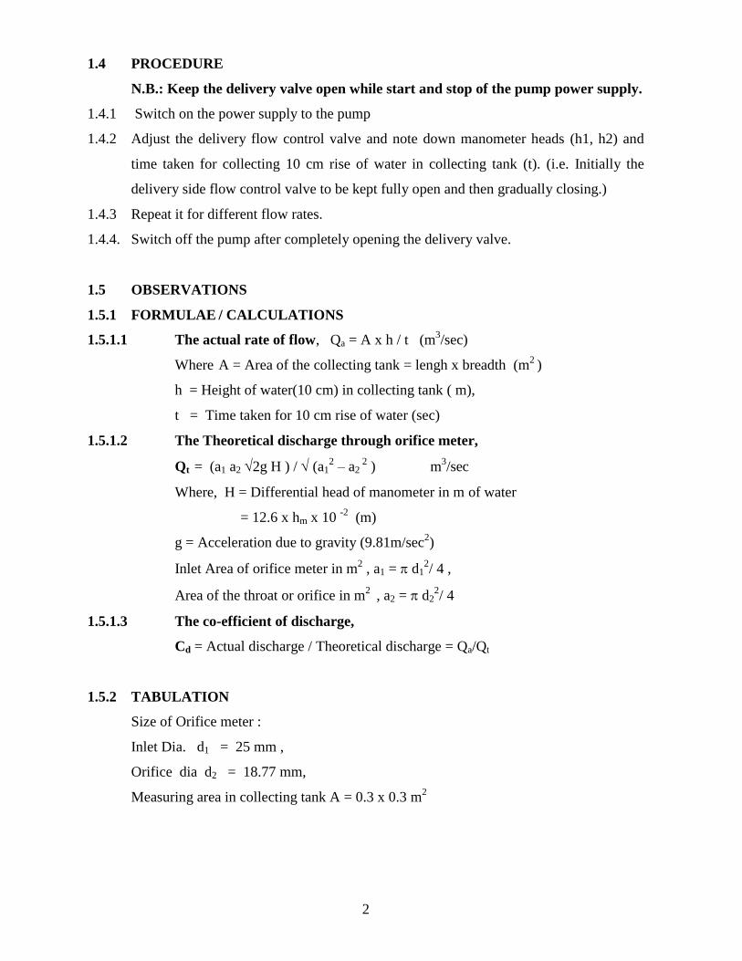
1.4 PROCEDURE
N.B.: Keep the delivery valve open while start and stop of the pump power supply.
1.4.1 Switch on the power supply to the pump
1.4.2 Adjust the delivery flow control valve and note down manometer heads (h1, h2) and
time taken for collecting 10 cm rise of water in collecting tank (t). (i.e. Initially the
delivery side flow control valve to be kept fully open and then gradually closing.)
1.4.3 Repeat it for different flow rates.
1.4.4. Switch off the pump after completely opening the delivery valve.
1.5 OBSERVATIONS
1.5.1 FORMULAE / CALCULATIONS
1.5.1.1 The actual rate of flow, Qa = A x h / t (m3/sec)
Where A = Area of the collecting tank = lengh x breadth (m2
)
h = Height of water(10 cm) in collecting tank ( m),
t = Time taken for 10 cm rise of water (sec)
1.5.1.2 The Theoretical discharge through orifice meter,
Qt = (a1 a2 2g H ) / (a12 – a2
2 ) m
3/sec
Where, H = Differential head of manometer in m of water
= 12.6 x hm x 10 -2
(m)
g = Acceleration due to gravity (9.81m/sec2)
Inlet Area of orifice meter in m2 , a1 = d1
2/ 4 ,
Area of the throat or orifice in m2
, a2 = d22/ 4
1.5.1.3 The co-efficient of discharge,
Cd = Actual discharge / Theoretical discharge = Qa/Qt
1.5.2 TABULATION
Size of Orifice meter :
Inlet Dia. d1 = 25 mm ,
Orifice dia d2 = 18.77 mm,
Measuring area in collecting tank A = 0.3 x 0.3 m2
3
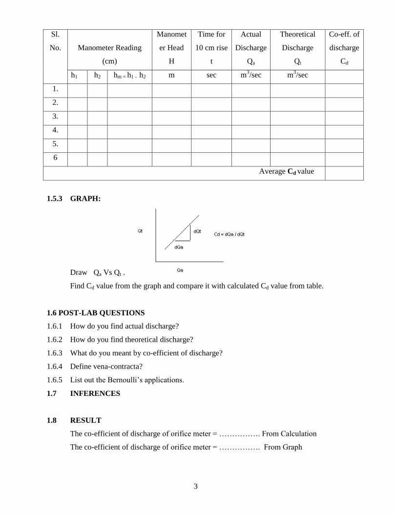
Sl.
No.
Manometer Reading
(cm)
Manomet
er Head
H
Time for
10 cm rise
t
Actual
Discharge
Qa
Theoretical
Discharge
Qt
Co-eff. of
discharge
Cd
h1 h2 hm = h1 - h2 m sec m3/sec m
3/sec
1.
2.
3.
4.
5.
6
Average Cd value
1.5.3 GRAPH:
Draw Qa Vs Qt .
Find Cd value from the graph and compare it with calculated Cd value from table.
1.6 POST-LAB QUESTIONS
1.6.1 How do you find actual discharge?
1.6.2 How do you find theoretical discharge?
1.6.3 What do you meant by co-efficient of discharge?
1.6.4 Define vena-contracta?
1.6.5 List out the Bernoulli’s applications.
1.7 INFERENCES
1.8 RESULT
The co-efficient of discharge of orifice meter = ……………. From Calculation
The co-efficient of discharge of orifice meter = ……………. From Graph
4
EXPERIMENT No.2
FLOW MEASUREMENT BY VENTURIMETER
2.1 AIM: To determine the co-efficient of discharge of the venturimeter
2.2 EQUIPMENTS REQUIRED: Venturimeter test rig, Stopwatch
2.3 PREPARATION
2.3.1 THEORY
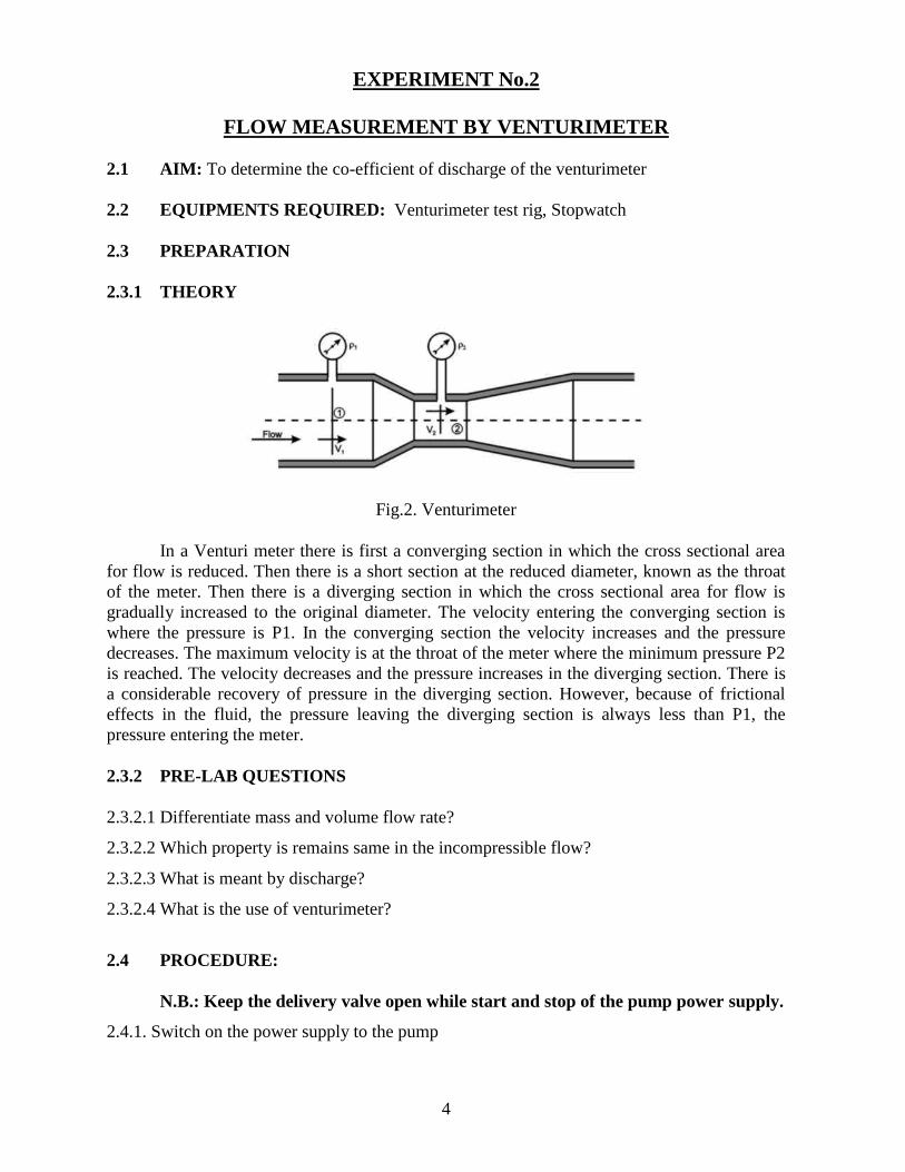
Fig.2. Venturimeter
In a Venturi meter there is first a converging section in which the cross sectional area
for flow is reduced. Then there is a short section at the reduced diameter, known as the throat
of the meter. Then there is a diverging section in which the cross sectional area for flow is
gradually increased to the original diameter. The velocity entering the converging section is
where the pressure is P1. In the converging section the velocity increases and the pressure
decreases. The maximum velocity is at the throat of the meter where the minimum pressure P2
is reached. The velocity decreases and the pressure increases in the diverging section. There is
a considerable recovery of pressure in the diverging section. However, because of frictional
effects in the fluid, the pressure leaving the diverging section is always less than P1, the
pressure entering the meter.
2.3.2 PRE-LAB QUESTIONS
2.3.2.1 Differentiate mass and volume flow rate?
2.3.2.2 Which property is remains same in the incompressible flow?
2.3.2.3 What is meant by discharge?
2.3.2.4 What is the use of venturimeter?
2.4 PROCEDURE:
N.B.: Keep the delivery valve open while start and stop of the pump power supply.
2.4.1. Switch on the power supply to the pump
5
2.4.2. Adjust the delivery flow control valve and note down manometer heads (h1, h2) and
time taken for collecting 10 cm rise of water in collecting tank (t). (i.e. Initially the
delivery side flow control valve to be kept fully open and then gradually closing.)
2.4.3. Repeat it for different flow rates.
2.4.4. Switch off the pump after completely opening the delivery valve.
2.5 OBSERVATIONS
2.5.1 FORMULAE / CALCULATIONS
2.5.1.1 The actual rate of flow, Qa = A x h / t (m3/sec)
Where A = Area of the collecting tank = lengh x breadth (m2
)
h = Height of water(10 cm) in collecting tank ( m),
t = Time taken for 10 cm rise of water (sec)
2.5.1.2 The Theoretical discharge through venturimeter,
Qt = (a1 a2 2g H ) / (a12 – a2
2 ) m
3/sec
Where, H = Differential head of manometer in m of water
= 12.6 x hm x 10 -2
(m)
g = Acceleration due to gravity (9.81m/sec2)
Inlet Area of venturimeter in m2 , a1 = d1
2/ 4 ,
Area of the throat in m2
, a2 = d22/ 4
2.5.1.3 The co-efficient of discharge,
Cd = Actual discharge / Theoretical discharge = Qa/Qt
2.5.2 TABULATION:
Inlet Dia. of Venturimeter (or) Dia of Pipe d1 = 25 mm
Throat diameter of Venturimeter d2 = 18.79 mm
Area of collecting tank , A = Length x Breadth = 0.3 x 0.3m2
6
Sl.
No.
Manometer Reading
(cm)
Mano-
meter
Head
H
Time for
10 cm
rise
t
Actual
Discharge
Qa
Theoretical
Discharge
Qt
Co-eff. of
discharge
Cd
h1 h2 hm = h1 - h2 m sec m3/sec m
3/sec
1.
2.
3.
4.
5.
Average Cd value
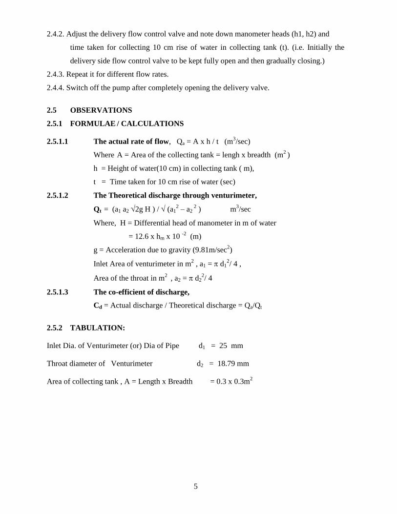
2.5.3 GRAPH:
Draw Qa Vs Qt .
Find Cd value from the graph and compare it with calculated Cd value from table.
2.6 POST-LAB QUESTIONS
2.6.1 How do you find actual and theoretical discharge?
2.6.2 What do you meant by throat of the venturimeter?
2.6.3 List out the practical applications of Bernoulli’s equation?
2.6.4 What is the use of U-tube manometer?
2.7 INFERENCES
2.8 RESULT
The co-efficient of discharge of Venturi meter = ……………. From Calculation
The co-efficient of discharge of Venturi meter = ……………. From Graph

7
EXPERIMENT No.3
VERIFICATION OF BERNOULLIS THEOREM
3.1 AIM: To verify the Bernoulli’s theorem
3.2 EQUIPMENTS REQUIRED: Bernoulli’s Theorem test set-up, Stopwatch
3.3 PREPARATION
3.3.1 THEORY
Bernoulli’s Theorem
According to Bernoulli’s Theorem, in a continuous fluid flow, the total head at any
point along the flow is the same. Z1 + P1/ g +V12/2g= Z2 + P2/ g +V2
2/2g , Since Z1 –Z2 = 0
for Horizontal flow, h1 +V12/2g= h2 +V2
2/2g ( Pr. head, h = P1/ g ). Z is ignored for adding in
both sides of the equations due to same datum for all the positions.
3.3.2 PRE-LAB QUESTIONS
3.3.2.1 State Bernoulli’s theorem?
3.3.2.2 What is continuity equation?
3.3.2.3 What do you meant by potential head?
3.3.2.4 What do you meant by pressure head?
3.3.2.5 What do you meant by kinetic head?
3.4 PROCEDURE
N.B.: Keep the delivery valve open while start and stop of the pump power supply.
3.4.1 Switch on the pump power supply.
3.4.2 Fix a steady flow rate by operating the appropriate delivery valve and drain valve
3.4.3. Note down the pressure heads (h1 – h8) in meters
3.4.4. Note down the time taken for 10 cm rise of water in measuring (collecting) tank.
3.4.5. Switch off the power supply.
3.5 OBSERVATIONS
3.5.1 FORMULAE / CALCULATIONS
3.5.1.1 Rate of flow Q = Ah /t.
Where A: Area of measuring tank = Length x Breadth (m2)
h: Rise of water in collecting tank (m) .. (i.e. h = 10 cm )
t: Time taken for 10 cm rise of water in collecting tank (sec)
8
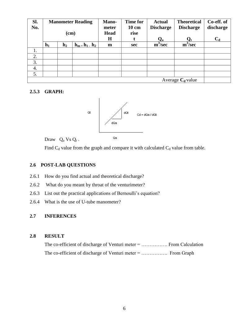
3.5.1.2 Velocity of flow, V = Q/a ,
Where a – Cross section area of the duct at respective peizometer positions (a1 - a8)
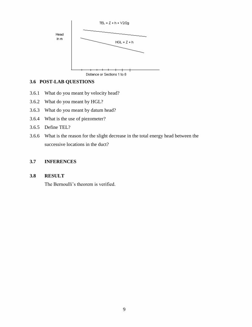
3.5.1.3 Hydraulic Gradient Line (HGL): It is the sum of datum and pressure at any point
HGL = Z + h
3.5.1.4 Total Energy Line (TEL): It is the sum of Pressure head and velocity head
TEL = Z + h +V2/2g
3.5.2 TABULATIONS
Area of measuring tank = 0.3 x 0.3 m2
Assume Datum head Z = 0
Diameter at the
sections of the
channel
d
Cross –
Section
Area
a = d2/ 4
Time
for 10
cm rise
t
Dischar
ge
Q=Ah/t
Velocity
V=Q/a Velocity
Head
V2/2g
Piezometer
Reading i.e.
Pr. Head
(h=P/g )
Total Head
Z +h+
V2/2g
m x10-3
m2 sec m
3/sec m/sec m m m
d1 = 0.04295
1.448
d2 = 0.03925
1.209
d3= 0.03555
0.992
d4= 0.03185
0.796
d5 = 0.02815
0.622
d6= 0.02445
0.469
d7= 0.02075
0.338
d8= 0.01705
0.228
3.5.3 GRAPH
Draw the graph: Distance of channel (Locations 1-8) Vs HGL, TEL
9
3.6 POST-LAB QUESTIONS
3.6.1 What do you meant by velocity head?
3.6.2 What do you meant by HGL?
3.6.3 What do you meant by datum head?
3.6.4 What is the use of piezometer?
3.6.5 Define TEL?
3.6.6 What is the reason for the slight decrease in the total energy head between the
successive locations in the duct?
3.7 INFERENCES
3.8 RESULT
The Bernoulli’s theorem is verified.
10
EXPERIMENT No.4
DETERMINATION OF PIPE FRICTION FACTOR
4.1 AIM: To determine the friction factor for the given pipe.
4.2 EQUIPMENTS REQUIRED: Pipe friction EQUIPMENTS, Stop watch
4.3 PREPARATION
4.3.1 THEORY
The major loss in the pipe is due to the inner surface roughness of the pipe. There
are three pipes (diameter 25 mm, 20 mm and 15 mm) available in the experimental set
up. The loss of pressure head is calculated by using the manometer. The apparatus is
primarily designed for conducting experiments on the frictional losses in pipes of
different sizes. Three different sizes of pipes are provided for a wide range of
experiments.
4.3.2 PRE-LAB QUESTIONS
4.3.2.1. What do you meant by friction and list out its effects?
4.3.2.2 What do you meant by major loss in pipe?
4.3.2.3 Write down the Darcy-Weisbach equation?
4.3.2.4 What are the types of losses in pipe flow?
4.4 PROCEDURE
N.B.: Keep the delivery valve open while start and stop of the pump power supply.
4.4.1. Switch on the pump and choose any one of the pipe and open its corresponding
inlet and exit valves to the manometer.
4.4.2. Adjust the delivery control valve to a desired flow rate. (i.e. fully opened
delivery valve position initially)
4.4.3 Take manometer readings and time taken for 10 cm rise of water in the collecting
tank
4.4.4 Repeat the readings for various flow rates by adjusting the delivery valve. (i.e.
Gradually closing the delivery valve from complete opening)
4.4.5 Switch of the power supply after opening the valve completely at the end.

11
4.5 OBSERVATIONS
4.5.1 FORMULAE / CALCULATIONS
4.5.1.1 The actual rate of flow Q = A x h / t (m3/sec)
Where A = Area of the collecting tank = lengh x breadth (m2
)
h = Height of water(10 cm) in collecting tank ( m),
t = Time taken for 10 cm rise of water (sec)
4.5.1.2 Head loss due to friction, hf = hm ( Sm – Sf)/ (Sf x 100) in m
hf = hm (13.6 – 1 ) x 10 -2
(m)
Where Sm = Sp. Gr. of manometric liquid , Hg =13.6 ,
Sf = Sp. Gr. of flowing liquid, H2O = 1
hm = Difference in manometric reading = (h1-h2) in cm
4.5.1.3 The frictional loss of head in pipes (Darcy-Weisbach formula)
hf = 4f L V2
2 g d
Where f = Co-efficient of friction or friction factor for the pipe (to be found)
L = Distance between two sections for which loss of head is measured = 3 m
V = Average Velocity of flow = Q/a (m/s),
Area of pipe a= d2/ 4 (m
2),
d = Pipe diameter = 0.015 m
g = Acceleration due to gravity = 9.81 m/sec2
4.5.2 TABULATION
Length between Pressure tapping, L = 3 m
Pipe Diameter, d = 0.015 m,
Measuring tank area, A= 0.6 x 0.3m2 ,
Sl.No. Pipe
Dia
Manometer
Reading
Head
Loss
Time
for 10
cm rise
Discharg
e
Velocit
y
Frictional
factor
d h1 h2 hm =
(h1-h2)
hf T Q V=Q/a f
m cm M Sec m3/s m/s
1
2
3
4
5
Average friction factor, f

12
4.5.3 GRAPH
Draw the graph: Q Vs hf
4.6 POST-LAB QUESTIONS
4.6.1 What is the relationship between friction head loss and pipe diameter?
4.6.2 What is the relationship between friction head loss and flow velocity?
4.6.3 What is the relationship between friction head loss and pipe length?
4.6.4 How is the flow rate and head loss related?
4.6.5 If flow velocity doubles, what happen to the frictional head loss?
4.7 INFERENCES
4.8 RESULT
The friction factor for the given pipe diameter of ……… m is = __________
13
EXPERIMENT No.5
DETERMINATION OF MINOR LOSSES DUE TO PIPE FITTINGS
9.1 AIM: To study the various losses due to the pipe fittings
9.2 EQUIPMENTS REQUIRED: Minor losses test rig, Stopwatch
9.3 PREPARATION
9.3.1 THEORY
The various pipe fittings used in the piping applications are joints, bends,
elbows, entry, exit and sudden flow area changes (enlargement and contraction)
etc. The energy losses associated with these types of pipe fittings are termed as
the minor losses due its lesser values compared to the major loss (pipe friction) in
the pipe. The loss of head is indicated by the manometer connected across the
respective pipe fitting.
9.3.2 PRE-LAB QUESTIONS
9.3.2.1 List out the various types of pipe fittings?
9.3.2.2 What do you meant by minor losses?
9.3.2.3 What are the types of losses in pipe flow?
9.3.2.4 What do you meant by entry loss?
9.3.2.5 What do you meant by exit loss?
9.4 PROCEDURE
N.B.: Keep the delivery valve open while start and stop of the pump power supply.
9.4.1 Switch on the pump. Adjust the delivery valve to a desired steady flow rate.
9.4.2 Note down the time taken for 10 cm rise of water level in the collecting tank.
9.4.3 Choose any one of the pipe fittings (2 bends, one enlargement and one
contraction). e.g. Bend-1
9.4.4 Open the levers (cocks) of respective pipe fitting to the manometer. Ensure other
fitting levers should be closed. e.g. Open the entry and exit levers of Bend-1( left
& right side cocks at the top of the panel)
9.4.5 Note down the manometer head levels (e.g. h1 & h2 for bend-1)
9.4.6 Now open the other two entry and exit levers of next pipe fitting. Then close the
levers of first chosen pipe fitting. (e.g. Open the 2nd
left & right levers for Bend-2
and close the top levers of Bend-1)
9.4.7 Note down the manometer for the second pipe fitting. (e.g. h1 & h2 for bend-2)

14
9.4.8 Repeat this procedure by opening the respective levers of sudden enlargement
fitting after closing other levers( i.e. for sudden enlargement by opening the next
down left & right cocks of sudden enlargement and then close the previous left &
right cocks of Bend-2).
9.4.9 Repeat this procedure by opening the respective levers of sudden contraction
fitting after closing other levers( i.e. for sudden contraction by opening the next
down left & right cocks of sudden contraction and then close the previous left &
right cocks of Sudden enlargement).
9.4.10 Ensure the readings taken for all pipe fittings and then switch off the pump.
9.5 OBSERVATIONS
9.5.1 FORMULAE / CALCULATIONS
9.5.1.1. Discharge, Q = (A x h ) / t ….. (m3/s)
A = Area of tank in m2
,
h = 0.10 m // Rise water level in collecting tank (m),
t = Time taken for the 10 cm rise of water in collecting tank (sec)
9.5.1.2. Velocity, V = Discharge / Area of pipe = Q/A… (m/s)
Where A = d2/4 , d – Dia of pipe in m
9.5.1.3. Actual loss of head, hf = ( h1 – h2 ) x 12.6 x 10⁻²
… (m)
9.5.1.4. Theoretical Velocity loss heads for pipe fittings
Velocity head loss for bend and elbow hv = V2 / (2g)
Velocity head loss for sudden enlargement hv = ( V1 – V2 )2 / (2g)
Velocity head loss for sudden contraction hv = 0.5 (V2)2 / (2g)
Where V2= velocity of smaller pipe
9.5.1.5. Loss co-efficient K = Theoretical Velocity head /Actual loss of head = hv / hf
15
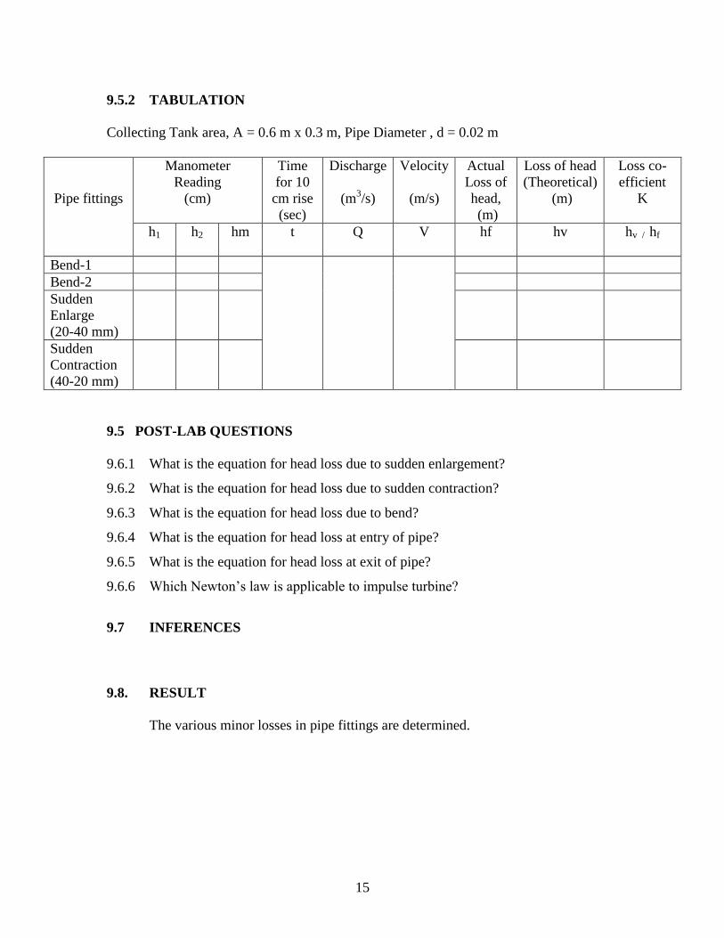
9.5.2 TABULATION
Collecting Tank area, A = 0.6 m x 0.3 m, Pipe Diameter , d = 0.02 m
Pipe fittings
Manometer
Reading
(cm)
Time
for 10
cm rise
(sec)
Discharge
(m3/s)
Velocity
(m/s)
Actual
Loss of
head,
(m)
Loss of head
(Theoretical)
(m)
Loss co-
efficient
K
h1 h2 hm t Q V hf hv
hv / hf
Bend-1
Bend-2
Sudden
Enlarge
(20-40 mm)
Sudden
Contraction
(40-20 mm)
9.5 POST-LAB QUESTIONS
9.6.1 What is the equation for head loss due to sudden enlargement?
9.6.2 What is the equation for head loss due to sudden contraction?
9.6.3 What is the equation for head loss due to bend?
9.6.4 What is the equation for head loss at entry of pipe?
9.6.5 What is the equation for head loss at exit of pipe?
9.6.6 Which Newton’s law is applicable to impulse turbine?
9.7 INFERENCES
9.8. RESULT
The various minor losses in pipe fittings are determined.
16
EXPERIMENT No.6
IMPACT OF JET OF WATER ON VANES
13.1 AIM: To determine the coefficient of impact of water jet on different vanes
13.2 EQUIPMENTS REQUIRED: Jet on vane apparatus, Weighing machine, Flat
vane, Flat vane with oblique impact, Conical vane, stop watch
13.3 PREPARATION
13.3.1 THEORY
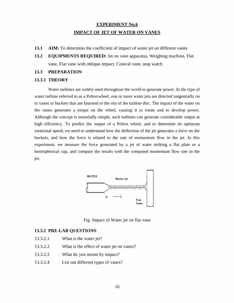
Water turbines are widely used throughout the world to generate power. In the type of
water turbine referred to as a Pelton
wheel, one or more water jets are directed tangentially on
to vanes or buckets that are fastened to the rim of the turbine disc. The impact of the water on
the vanes generates a torque on the wheel, causing it to rotate and to develop power.
Although the concept is essentially simple, such turbines can generate considerable output at
high efficiency. To predict the output of a Pelton wheel, and to determine its optimum
rotational speed, we need to understand how the deflection of the jet generates a force on the
buckets, and how the force is related to the rate of momentum flow in the jet. In this
experiment, we measure the force generated by a jet of water striking a flat plate or a
hemispherical cup, and compare the results with the computed momentum flow rate in the
jet.
Fig. Impact of Water jet on flat vane
13.3.2 PRE-LAB QUESTIONS
13.3.2.1 What is the water jet?
13.3.2.2 What is the effect of water jet on vanes?
13.3.2.3 What do you meant by impact?
13.3.2.4 List out different types of vanes?
17
13.4 PROCEDURE
13.4.1 Switch on the power supply.
13.4.2 Open the gate valve and note down the reading from the weight balance.
13.4.3 Then note the time for ‘h’ m rise in collecting tank.
13.4.4 Repeat the procedure for different gate valve openings.
13.4.5 Take readings for different vanes and nozzles also.
13.5 OBSERVATIONS
13.5.1 FORMULAE / CALCULATIONS
13.5.1.1 Actual discharge, Q = Volume of collecting tank/ time taken = A h / t
Where, A - Area of collecting tank = length x breadth
h - Water level rise in the collecting tank = 10 cm
t - Time taken for ‘h’ cm rise of water in the tank in sec
13.5.1.2 Theoretical force Ft = ( AN V 2)/ g
Density of water, = 1000 kg/m3
Area of nozzle, AN = d2/4
Gravity, g = 9.81 m/s2
13.5.1.3 Velocity V = Q/ [Cc. AN]
13.5.1.4 Co-efficient of Impact, Ci = Fa / Ft
Where Fa = Actual force acting on the Disc shown from Dial Gauge.
13.5.2 TABULATION
Measuring area in tank = 0.5 x 0.4 m2
Dia of jet = 15mm
Type of vane = Flat vane / Conical vane
Co-efficient of Contraction, Cc = 0.97
18
Sl.
No.
Type of Vane
Time for 10 cm
rise of water
(sec)
Actual
force,
Fa in kg
Theoretical
Force,
Ft in kg
Co-efficient
of impact,
Ci
1
2
3
4
5
6
13.5 POST-LAB QUESTIONS
13.6.1 How do you compare different vanes?
13.6.2 What do you meant by co-efficient of impact?
13.6.3 How do you measure the force of the jet?
13.6.4 How do you measure actual flow rate?
13.6.5 How do you measure theoretical flow rate?
13.7 INFERENCES
13.8 RESULT
The co-efficient of impact of the given vane = ___________
19
EXPERIMENT No.7
FLOW VISUALIZATION - REYNOLDS APPARATUS
14.1 AIM: To demonstrate the flow visualization – laminar or turbulent flow.
14.2 EQUIPMENTS REQUIRED: Reynolds Experimental set up, stop watch
14.3 PREPARATION
14.3.1 THEORY
The flow of real fluids can basically occur under two very different regimes
namely laminar and turbulent flow. The laminar flow is characterized by fluid particles
moving in the form of lamina sliding over each other, such that at any instant the velocity
at all the points in particular lamina is the same. The lamina near the flow boundary move
at a slower rate as compared to those near the center of the flow passage. This type of
flow occurs in viscous fluids , fluids moving at slow velocity and fluids flowing through
narrow passages. The turbulent flow is characterized by constant agitation and
intermixing of fluid particles such that their velocity changes from point to point and
even at the same point from time to time. This type of flow occurs in low density fluids,
flow through wide passage and in high velocity flows.
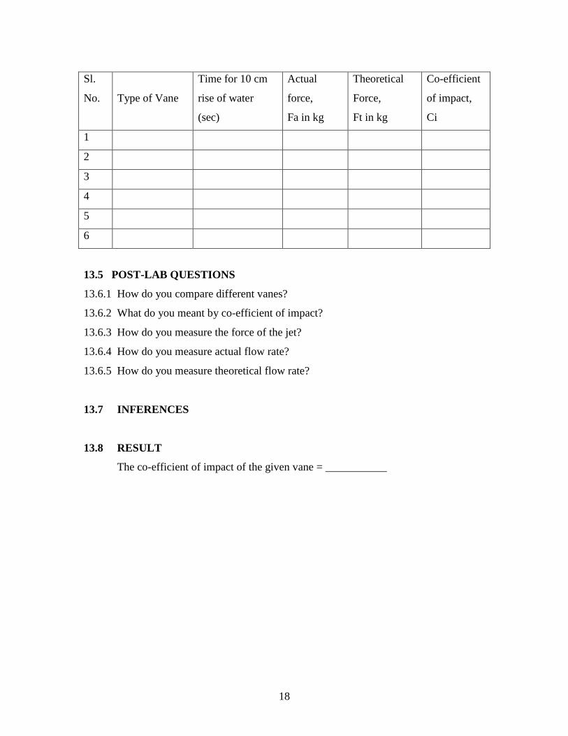
Fig. Reynolds Experimental Set-up
Reynolds conducted an experiment for observation and determination of these
regimes of flow. By introducing a fine filament of dye in to the flow of water through the
glass tube ,at its entrance he studied the different types of flow. At low velocities the dye
filament appeared as straight line through the length of the tube and parallel to its axis,
characterizing laminar flow. As the velocity is increased the dye filament becomes wavy
throughout indicating transition flow. On further increasing the velocity the filament
breaks up and diffuses completely in the water in the glass tube indicating the turbulent
flow. There are two different types of fluid flows laminar flow and Turbulent flow. The
velocity at which the flow changes laminar to Turbulent is called the ‘Critical Velocity’.
20
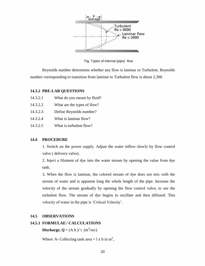
Fig. Types of internal (pipe) flow
Reynolds number determines whether any flow is laminar or Turbulent. Reynolds
number corresponding to transition from laminar to Turbulent flow is about 2,300.
14.3.2 PRE-LAB QUESTIONS
14.3.2.1 What do you meant by fluid?
14.3.2.2 What are the types of flow?
14.3.2.3 Define Reynolds number?
14.3.2.4 What is laminar flow?
14.3.2.5 What is turbulent flow?
14.4 PROCEDURE
1. Switch on the power supply. Adjust the water inflow slowly by flow control
valve ( delivery valve).
2. Inject a filament of dye into the water stream by opening the value from dye
tank.
3. When the flow is laminar, the colored stream of dye does not mix with the
stream of water and is apparent long the whole length of the pipe. Increase the
velocity of the stream gradually by opening the flow control valve, to see the
turbulent flow. The stream of dye begins to oscillate and then diffused. This
velocity of water in the pipe is ‘Critical Velocity’.
14.5 OBSERVATIONS
14.5.1 FORMULAE / CALCULATIONS
Discharge, Q = (A h )/ t (m3/sec)
Where A- Collecting tank area = l x b in m2,
21
t - time for 10 cm rise of water level in the collecting tank (sec)
h – Rise of water level in the collecting tank = 0.10 m
Reynolds number for pipe flow, Re = ( V D)/
Where V= Velocity of the fluid (m/s),
D= diameter of the pipe (m)
= Kinetic viscosity of the fluid (m2/s)
14.5.2 TABULATION
Internal plan area of collecting tank = 0.3 x 0.3m2
Diameter of pipe D = 32 mm , Kinematics viscosity of fluid (water) = 1.01 x 10⁻⁶
m2/sec
Sl. No. Time taken
for 10 cm
rise
t
sec
Discharge
Q
m3/sec
Velocity
V
m/s
Reynolds
number
Re
Remarks
(Laminar/
Turbulent
flow)
1
2
3
4
14.5 POST-LAB QUESTIONS
14.6.1 What do you meant by stream and streak lines?
14.6.2 Mention the Reynolds no for laminar and turbulent flow?
14.6.3 What do you meant by steady and unsteady flow?
14.6.4 What do you meant by path line?
14.6.5 What do you meant by uniform and non-uniform flow?
14.7 INFERENCES
14.8 RESULT
The flow visualization test is conducted.