1

Experiment No. 01

MEASUREMENT OF CAPPILARY RISE

Aim

To measure capillary rise produced in capillary tubes of different sizes and compare it

with the estimated values.

Apparatus

Glass capillary tubes of different diameters, measuring scale and given liquid.

Theory

The liquid has greater adhesion than cohesion, thus it wets the solid surface with which it

is in contact and also tends to rise at the point of contact with the result that the liquid

surface is concave upward and angle of contact θ is less than 90• .The phenomenon of rise

or fall of liquid surface relative to the adjacent general level of liquid is known as

capillarity. The capillary rise can be determined by considering the condition of

equilibrium in a circular tube of small diameter inserted in a liquid

Capillary Rise is given by, h= 4σ/ ρgd

where, h is the height of rise, σ is the surface tension, ρ is the density of the liquid and d

is the diameter of tube.

Procedure

i. Capillary tubes are well cleaned.

ii. Place the panel in the receiver with a certain level of water

iii. Place a cardboard between the capillary tubes.

iv. Mark the cardboard at the height of capillary rising in each tube.

v. Measure the capillary rise “H” in each tube

2

Fig. 1 Capillary rise in tubes of different diameter

Sample Calculation

Observation Table

S. No. Tube

diameter

(mm)

Capillary Rise

h (mm)

Observed Calculated

1

2

3

4

5

6

Results and Discussion

3

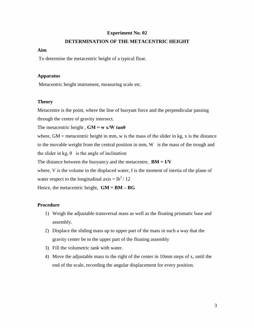
Experiment No. 02

DETERMINATION OF THE METACENTRIC HEIGHT

Aim

To determine the metacentric height of a typical float.

Apparatus

Metacentric height instrument, measuring scale etc.

Theory

Metacentre is the point, where the line of buoyant force and the perpendicular passing

through the centre of gravity intersect.

The metacentric height , GM = w x/W tanθ

where, GM = metacentric height in mm, w is the mass of the slider in kg, x is the distance

to the movable weight from the central position in mm, W is the mass of the trough and

the slider in kg, θ is the angle of inclination

The distance between the buoyancy and the metacentre, BM = I/V

where, V is the volume in the displaced water, I is the moment of inertia of the plane of

water respect to the longitudinal axis = lb3

/ 12

Hence, the metacentric height, GM = BM – BG

Procedure

1) Weigh the adjustable transversal mass as well as the floating prismatic base and

assembly.

2) Displace the sliding mass up to upper part of the mass in such a way that the

gravity center be in the upper part of the floating assembly

3) Fill the volumetric tank with water.

4) Move the adjustable mass to the right of the center in 10mm steps of x, until the

end of the scale, recording the angular displacement for every position.

4

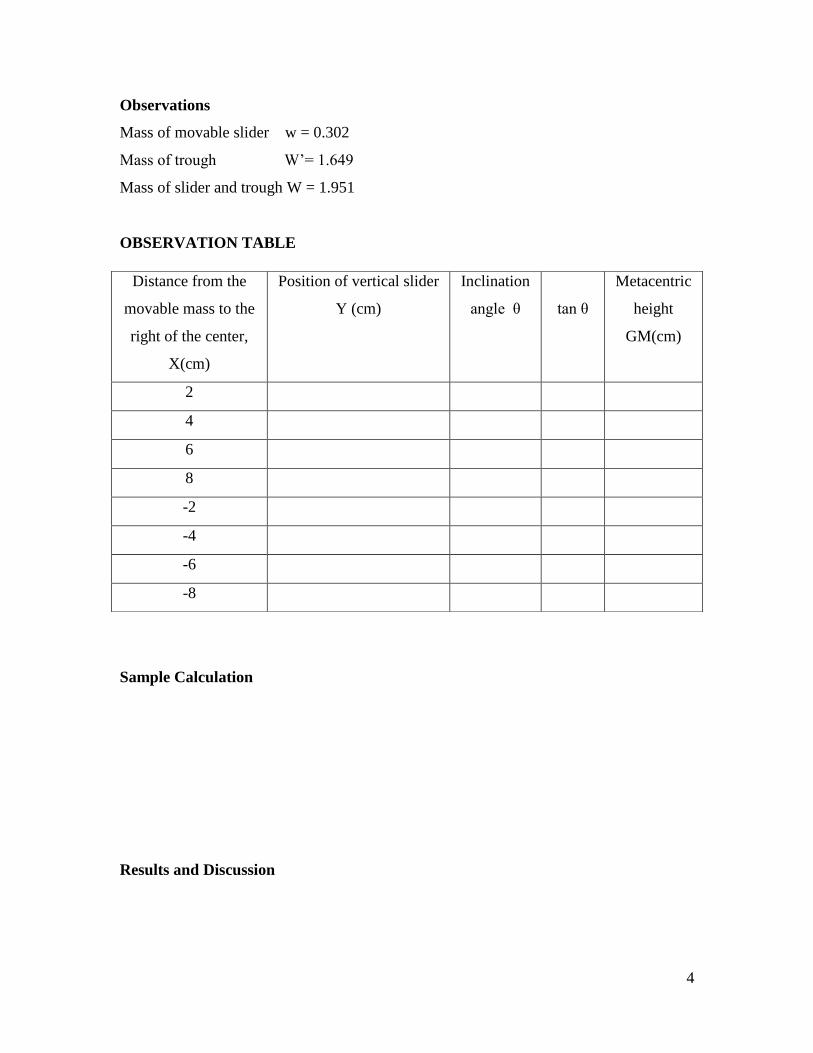
Observations

Mass of movable slider w = 0.302

Mass of trough W‟= 1.649

Mass of slider and trough W = 1.951

OBSERVATION TABLE

Sample Calculation

Results and Discussion

Distance from the

movable mass to the

right of the center,

X(cm)

Position of vertical slider

Y (cm)

Inclination

angle θ

tan θ

Metacentric

height

GM(cm)

2

4

6

8

-2

-4

-6

-8

5

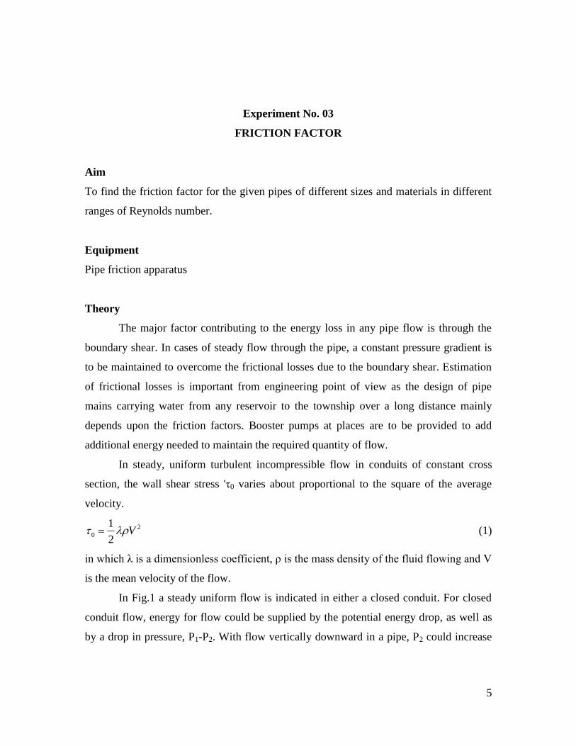
Experiment No. 03

FRICTION FACTOR

Aim

To find the friction factor for the given pipes of different sizes and materials in different

ranges of Reynolds number.

Equipment

Pipe friction apparatus

Theory

The major factor contributing to the energy loss in any pipe flow is through the

boundary shear. In cases of steady flow through the pipe, a constant pressure gradient is

to be maintained to overcome the frictional losses due to the boundary shear. Estimation

of frictional losses is important from engineering point of view as the design of pipe

mains carrying water from any reservoir to the township over a long distance mainly

depends upon the friction factors. Booster pumps at places are to be provided to add

additional energy needed to maintain the required quantity of flow.

In steady, uniform turbulent incompressible flow in conduits of constant cross

section, the wall shear stress 'τ0 varies about proportional to the square of the average

velocity.

2

0

1

2V (1)

in which λ is a dimensionless coefficient, ρ is the mass density of the fluid flowing and V

is the mean velocity of the flow.

In Fig.1 a steady uniform flow is indicated in either a closed conduit. For closed

conduit flow, energy for flow could be supplied by the potential energy drop, as well as

by a drop in pressure, P1-P2. With flow vertically downward in a pipe, P2 could increase

6

in the flow direction but potential energy drop Zl- Z2 would have to be greater than (p1-

p2)/γ to supply energy to overcome the wall shear stress.

Fig. 1 Axial Forces on Control Volume of Fluid Flowing

The linear momentum equation applied between sections 1 and 2 in the direction of flow

yields.

1 1 2 00 ( )F p p A ALSin LP (2)

in which P is the wetted perimeter of the conduit, that is the portion of the perimeter

where the wall is in contact with the fluid, A is the area of cross section of flow, L is the

distance between the two sections, γ is the specific weight of the liquid flowing and is

the inclination of the bed of the channel in the section 1 and 2 yields.

2 2

1 1 2 21 2

2 2f

P V P VZ Z h

g g

(3)

where hf is the head loss between sections 1 and 2. Since the velocity head is same i.e.

2 2

1 2

2 2

V V

g g , we have,

1 21 2f

P Ph Z Z

(4)

since L Sin -Z2), from Eq.2, it can be written as

1 21 2

P P LPZ Z

A

(5)

From Eq. 4 and 5

20 1

2f

LP LPh V

A A

(6)

7

2

2f

L Vh

R g (7)

where R is the hydraulic radius= A/P. For circular pipes, R=D/4. The unit of hf is meter-

Newton/Newton. After solving for V, we have

2gV RS C RS

(8)

For pipes, =f/4 and R= D/4, then

2

2f

LVh f

gD (9)

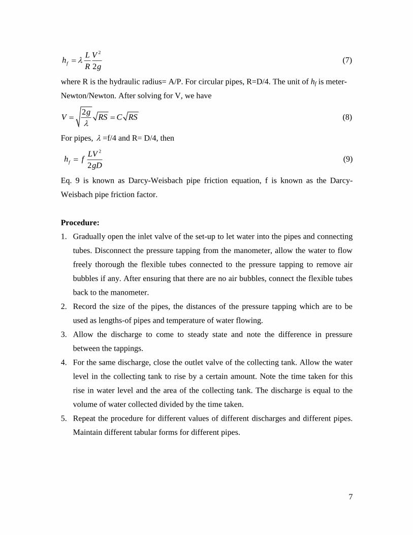
Eq. 9 is known as Darcy-Weisbach pipe friction equation, f is known as the Darcy-

Weisbach pipe friction factor.

Procedure:

1. Gradually open the inlet valve of the set-up to let water into the pipes and connecting

tubes. Disconnect the pressure tapping from the manometer, allow the water to flow

freely thorough the flexible tubes connected to the pressure tapping to remove air

bubbles if any. After ensuring that there are no air bubbles, connect the flexible tubes

back to the manometer.

2. Record the size of the pipes, the distances of the pressure tapping which are to be

used as lengths-of pipes and temperature of water flowing.

3. Allow the discharge to come to steady state and note the difference in pressure

between the tappings.

4. For the same discharge, close the outlet valve of the collecting tank. Allow the water

level in the collecting tank to rise by a certain amount. Note the time taken for this

rise in water level and the area of the collecting tank. The discharge is equal to the

volume of water collected divided by the time taken.

5. Repeat the procedure for different values of different discharges and different pipes.

Maintain different tabular forms for different pipes.

8

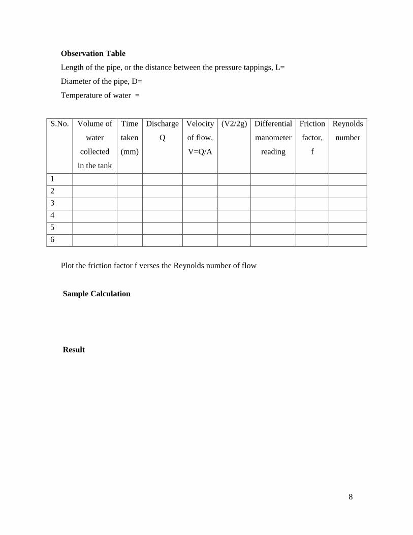
Observation Table

Length of the pipe, or the distance between the pressure tappings, L=

Diameter of the pipe, D=

Temperature of water =

S.No. Volume of

water

collected

in the tank

(mm)

Time

taken

(mm)

Discharge

Q

Velocity

of flow,

V=Q/A

(V2/2g)

Differential

manometer

reading

Friction

factor,

f

Reynolds

number

1

2

3

4

5

6

Plot the friction factor f verses the Reynolds number of flow

Sample Calculation

Result

9

Experiment No. 04

IMPACT OF A JET

OBJECTIVE:

To measure the force exerted by a jet on a flat plate normal to the Jet

APPARATUS

Impact of Jet Apparatus

Theory

A jet of fluid emerging from a nozzle has some velocity and hence it possesses a certain

amount of kinetic energy. If this jet strikes an obstruction placed in its path, it will exert a

force on the obstruction. This impressed force is known as impact of the jet. Since, a

dynamic force is involved by virtue of fluid motion; it always involves a change of

momentum.

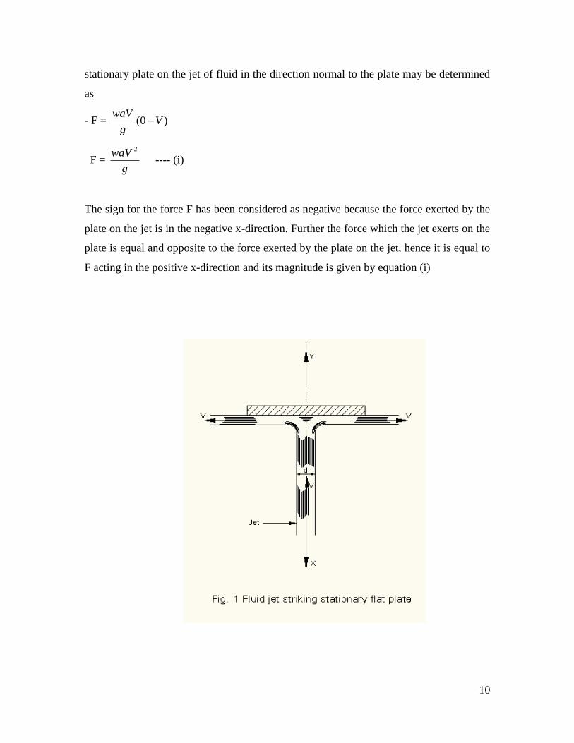
Flat plate normal to the jet: Let a jet of diameter d and velocity V is issued from a

nozzle and strikes a flat plate as shown in Fig 1. The plate is held stationary and

perpendicular to the centre line of the jet. The jet after striking the plate will leave it

tangentially i.e. the jet will get deflected through 900.

The quantity of fluid striking the plate Q= (πd2/ 4) x V = a V, where a is the area of cross

section of the jet. Thus, the mass of fluid issued by the jet per second is m = ρ Q = ρaV;

where ρ represents the mass density of the fluid. Since ρ = g

w(w/g), where w is the

specific weight of the fluid, the mass m may also be expressed as m = g

waV

After striking the plate since the jet gets deflected through 900, the component of the

velocity of the jet leaving the plate, in the original direction of the striking jet will be

zero. Therefore, by applying impulse-momentum equation, the force F exerted by the

10

stationary plate on the jet of fluid in the direction normal to the plate may be determined

as

­ F = )0( Vg

waV

F = g

waV 2

---- (i)

The sign for the force F has been considered as negative because the force exerted by the

plate on the jet is in the negative x-direction. Further the force which the jet exerts on the

plate is equal and opposite to the force exerted by the plate on the jet, hence it is equal to

F acting in the positive x-direction and its magnitude is given by equation (i)

11

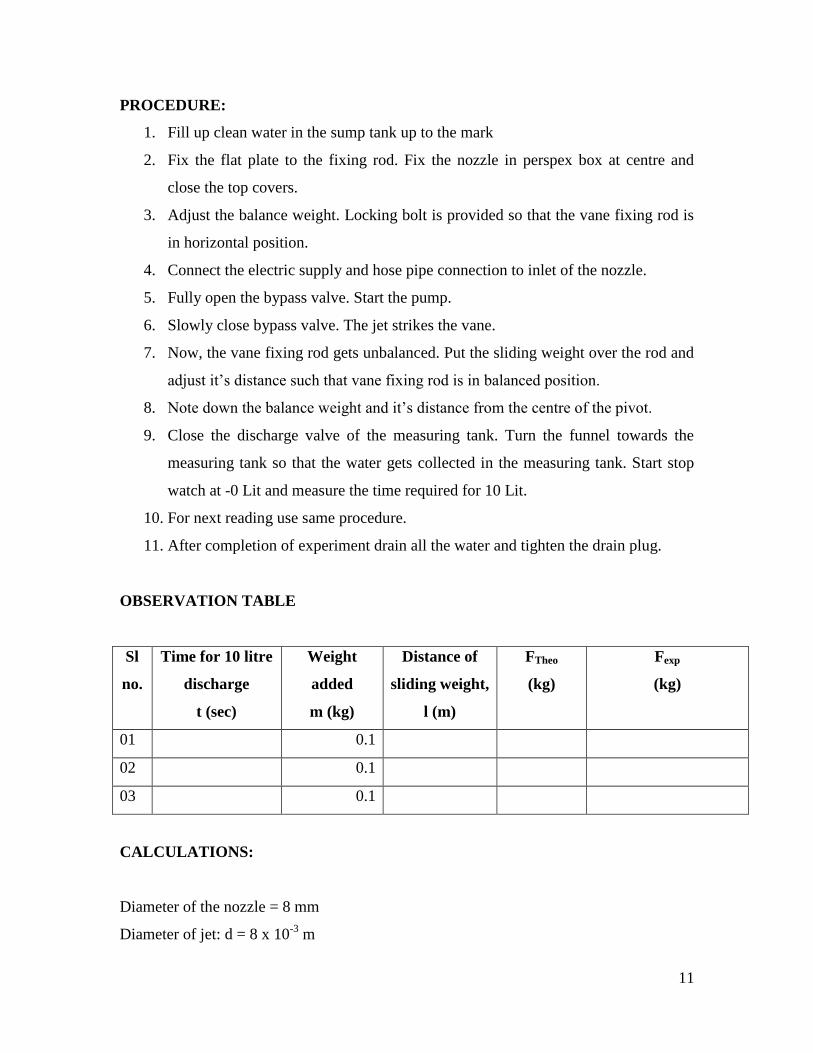
PROCEDURE:

1. Fill up clean water in the sump tank up to the mark

2. Fix the flat plate to the fixing rod. Fix the nozzle in perspex box at centre and

close the top covers.

3. Adjust the balance weight. Locking bolt is provided so that the vane fixing rod is

in horizontal position.

4. Connect the electric supply and hose pipe connection to inlet of the nozzle.

5. Fully open the bypass valve. Start the pump.

6. Slowly close bypass valve. The jet strikes the vane.

7. Now, the vane fixing rod gets unbalanced. Put the sliding weight over the rod and

adjust it‟s distance such that vane fixing rod is in balanced position.

8. Note down the balance weight and it‟s distance from the centre of the pivot.

9. Close the discharge valve of the measuring tank. Turn the funnel towards the

measuring tank so that the water gets collected in the measuring tank. Start stop

watch at -0 Lit and measure the time required for 10 Lit.

10. For next reading use same procedure.

11. After completion of experiment drain all the water and tighten the drain plug.

OBSERVATION TABLE

Sl

no.

Time for 10 litre

discharge

t (sec)

Weight

added

m (kg)

Distance of

sliding weight,

l (m)

FTheo

(kg)

Fexp

(kg)

01 0.1

02 0.1

03 0.1

CALCULATIONS:

Diameter of the nozzle = 8 mm

Diameter of jet: d = 8 x 10-3

m

12

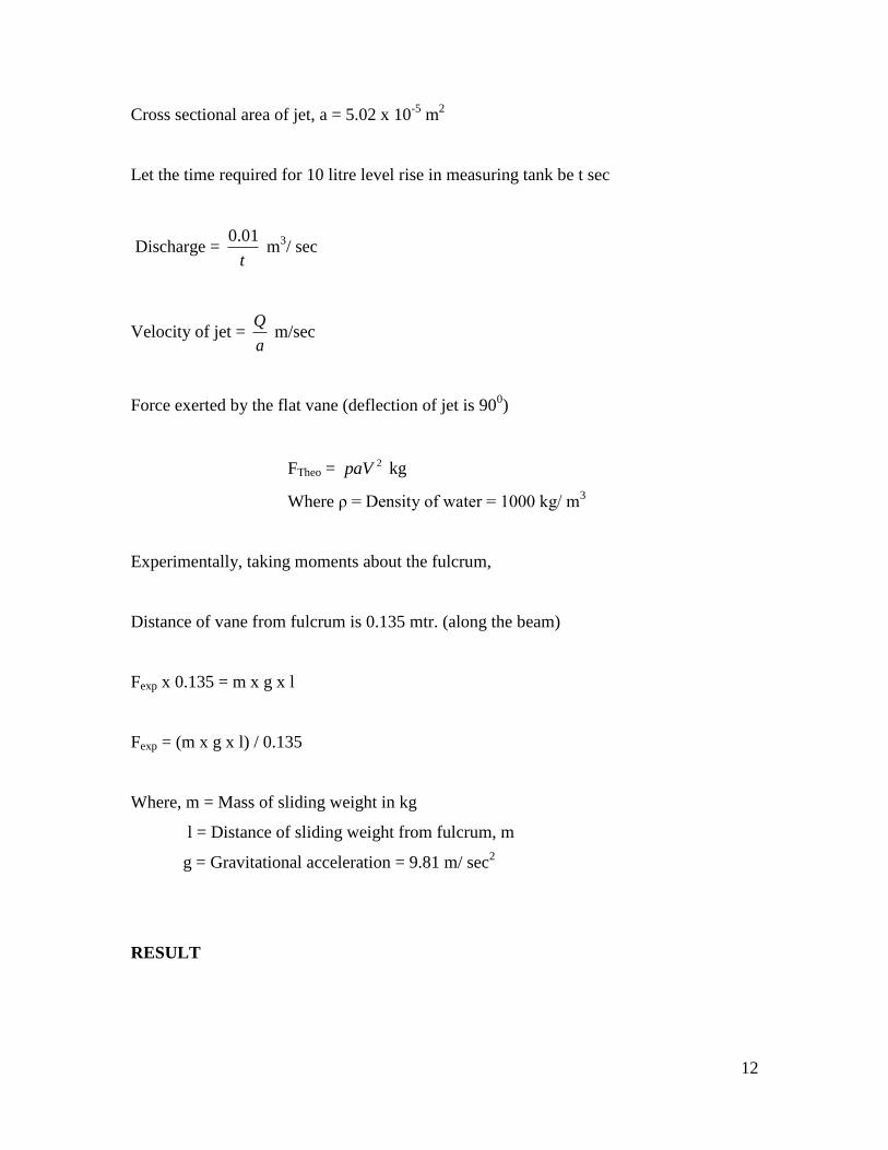
Cross sectional area of jet, a = 5.02 x 10-5

m2

Let the time required for 10 litre level rise in measuring tank be t sec

Discharge = t

01.0 m

3/ sec

Velocity of jet = a

Q m/sec

Force exerted by the flat vane (deflection of jet is 900)

FTheo = 2paV kg

Where ρ = Density of water = 1000 kg/ m3

Experimentally, taking moments about the fulcrum,

Distance of vane from fulcrum is 0.135 mtr. (along the beam)

Fexp x 0.135 = m x g x l

Fexp = (m x g x l) / 0.135

Where, m = Mass of sliding weight in kg

l = Distance of sliding weight from fulcrum, m

g = Gravitational acceleration = 9.81 m/ sec2

RESULT

13

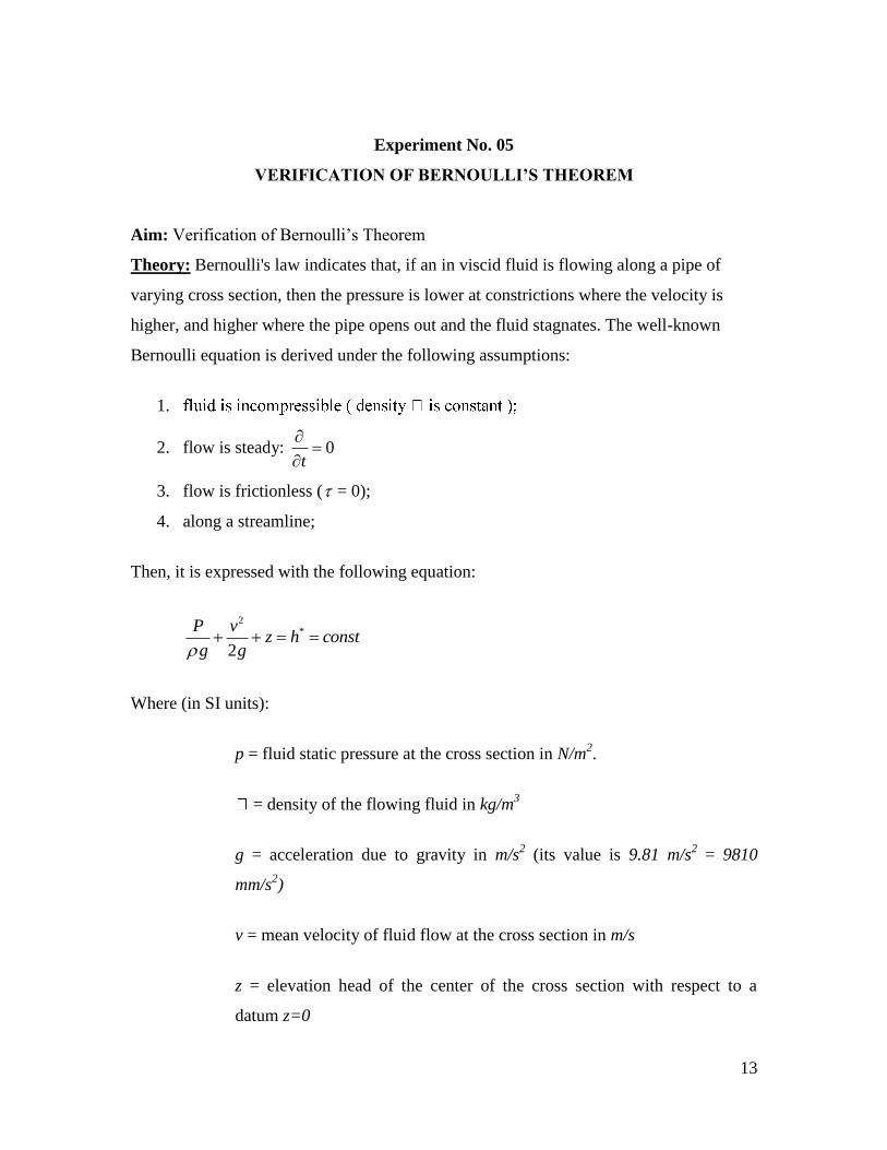
Experiment No. 05

VERIFICATION OF BERNOULLI’S THEOREM

Aim: Verification of Bernoulli‟s Theorem

Theory: Bernoulli's law indicates that, if an in viscid fluid is flowing along a pipe of

varying cross section, then the pressure is lower at constrictions where the velocity is

higher, and higher where the pipe opens out and the fluid stagnates. The well-known

Bernoulli equation is derived under the following assumptions:

1.

2. flow is steady: 0t

3. flow is frictionless ( = 0);

4. along a streamline;

Then, it is expressed with the following equation:

2

*

2

P vz h const

g g

Where (in SI units):

p = fluid static pressure at the cross section in N/m2.

= density of the flowing fluid in kg/m3

g = acceleration due to gravity in m/s2 (its value is 9.81 m/s

2 = 9810

mm/s2)

v = mean velocity of fluid flow at the cross section in m/s

z = elevation head of the center of the cross section with respect to a

datum z=0

14

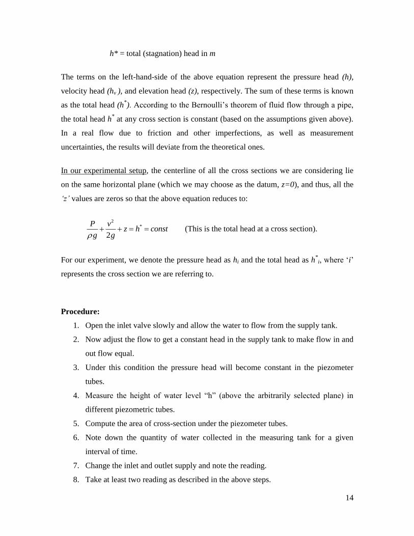
h* = total (stagnation) head in m

The terms on the left-hand-side of the above equation represent the pressure head (h),

velocity head (hv ), and elevation head (z), respectively. The sum of these terms is known

as the total head (h*). According to the Bernoulli‟s theorem of fluid flow through a pipe,

the total head h* at any cross section is constant (based on the assumptions given above).

In a real flow due to friction and other imperfections, as well as measurement

uncertainties, the results will deviate from the theoretical ones.

In our experimental setup, the centerline of all the cross sections we are considering lie

on the same horizontal plane (which we may choose as the datum, z=0), and thus, all the

‘z’ values are zeros so that the above equation reduces to:

2

*

2

P vz h const

g g (This is the total head at a cross section).

For our experiment, we denote the pressure head as hi and the total head as h*

i, where „i‟

represents the cross section we are referring to.

Procedure:

1. Open the inlet valve slowly and allow the water to flow from the supply tank.

2. Now adjust the flow to get a constant head in the supply tank to make flow in and

out flow equal.

3. Under this condition the pressure head will become constant in the piezometer

tubes.

4. Measure the height of water level “h” (above the arbitrarily selected plane) in

different piezometric tubes.

5. Compute the area of cross-section under the piezometer tubes.

6. Note down the quantity of water collected in the measuring tank for a given

interval of time.

7. Change the inlet and outlet supply and note the reading.

8. Take at least two reading as described in the above steps.

15

Experiment No. 6

ORIFICE

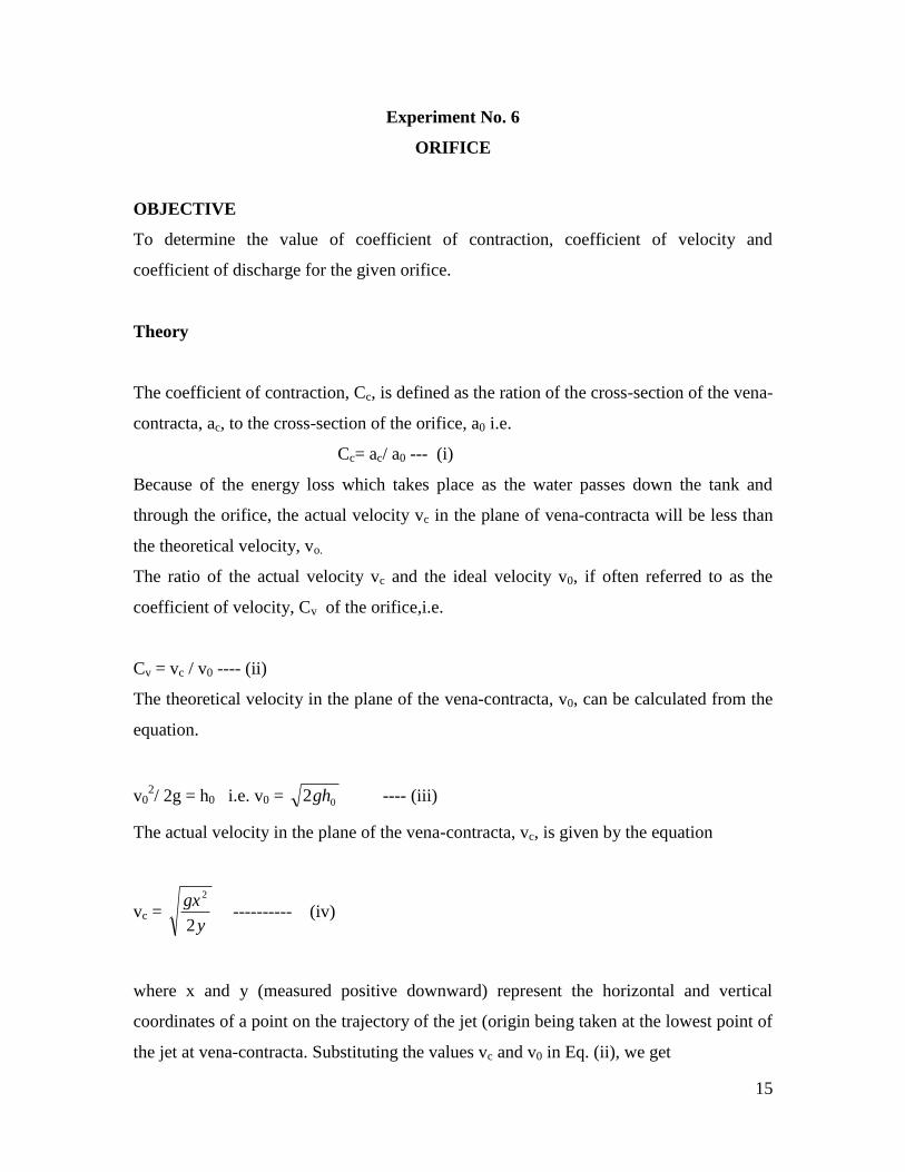
OBJECTIVE

To determine the value of coefficient of contraction, coefficient of velocity and

coefficient of discharge for the given orifice.

Theory

The coefficient of contraction, Cc, is defined as the ration of the cross-section of the vena-

contracta, ac, to the cross-section of the orifice, a0 i.e.

Cc= ac/ a0 --- (i)

Because of the energy loss which takes place as the water passes down the tank and

through the orifice, the actual velocity vc in the plane of vena-contracta will be less than

the theoretical velocity, vo.

The ratio of the actual velocity vc and the ideal velocity v0, if often referred to as the

coefficient of velocity, Cv of the orifice,i.e.

Cv = vc / v0 ---- (ii)

The theoretical velocity in the plane of the vena-contracta, v0, can be calculated from the

equation.

v02/ 2g = h0 i.e. v0 = 02gh ---- (iii)

The actual velocity in the plane of the vena-contracta, vc, is given by the equation

vc = y

gx

2

2

---------- (iv)

where x and y (measured positive downward) represent the horizontal and vertical

coordinates of a point on the trajectory of the jet (origin being taken at the lowest point of

the jet at vena-contracta. Substituting the values vc and v0 in Eq. (ii), we get

16

Cv = 0

2

4yh

x --------- (v)

Finally the coefficient of discharge, Cd, is defined as the ratio of the actual discharge to

that which would take place if the jet is discharged at the ideal velocity without reduction

of area. The actual discharge, Q, given by

Q= vcac ----------- (vi)

and can be measured with the help of measuring tank. And if the jet is discharged at the

ideal velocity v0 over the orifice area, a0, the discharge Q0 would be

Q0= v0a0

= 02gh a0 ----- (vii)

Thus, the coefficient of discharge is given by

Cd= 0Q

Q=

00 a

a

v

v cc = CcCV ----- (ix)

17

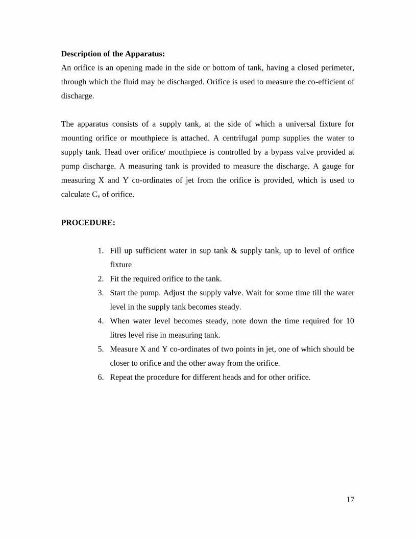
Description of the Apparatus:

An orifice is an opening made in the side or bottom of tank, having a closed perimeter,

through which the fluid may be discharged. Orifice is used to measure the co-efficient of

discharge.

The apparatus consists of a supply tank, at the side of which a universal fixture for

mounting orifice or mouthpiece is attached. A centrifugal pump supplies the water to

supply tank. Head over orifice/ mouthpiece is controlled by a bypass valve provided at

pump discharge. A measuring tank is provided to measure the discharge. A gauge for

measuring X and Y co-ordinates of jet from the orifice is provided, which is used to

calculate Cv of orifice.

PROCEDURE:

1. Fill up sufficient water in sup tank & supply tank, up to level of orifice

fixture

2. Fit the required orifice to the tank.

3. Start the pump. Adjust the supply valve. Wait for some time till the water

level in the supply tank becomes steady.

4. When water level becomes steady, note down the time required for 10

litres level rise in measuring tank.

5. Measure X and Y co-ordinates of two points in jet, one of which should be

closer to orifice and the other away from the orifice.

6. Repeat the procedure for different heads and for other orifice.

18

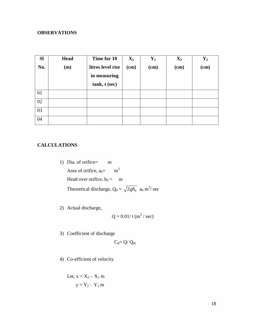
OBSERVATIONS

Sl

No.

Head

(m)

Time for 10

litres level rise

in measuring

tank, t (sec)

X1

(cm)

Y1

(cm)

X2

(cm)

Y2

(cm)

01

02

03

04

CALCULATIONS

1) Dia. of orifice= m

Area of orifice, a0= m2

Head over orifice, h0 = m

Theoretical discharge, Q0 = 02gh a0 m3/ sec

2) Actual discharge,

Q = 0.01/ t (m3 / sec)

3) Coefficient of discharge

Cd= Q/ Qth

4) Co-efficient of velocity

Let, x = X2 – X1 m

y = Y2 – Y1 m

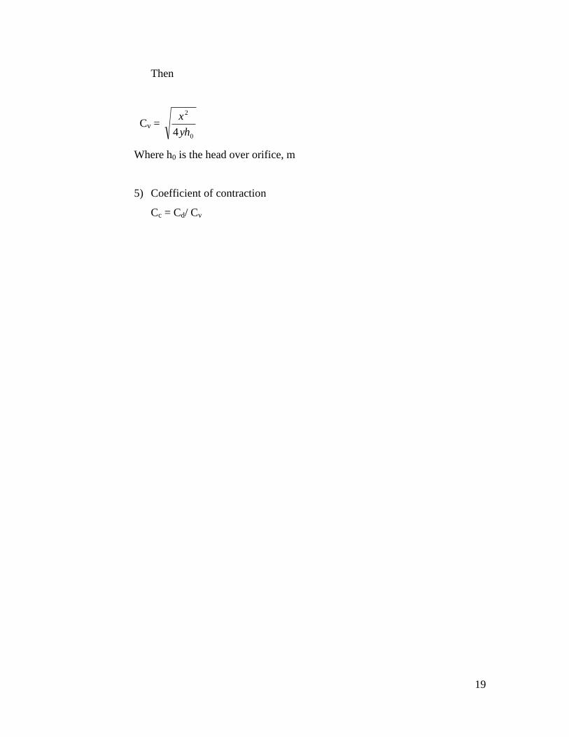
19

Then

Cv = 0

2

4yh

x

Where h0 is the head over orifice, m

5) Coefficient of contraction

Cc = Cd/ Cv

20

Experiment No. 07

Free and Forced vortex

OBJECTIVE

To determine the surface profile of a vortex apparatus.

Theory

When a liquid contained in a cylindrical vessel is given the rotation either due to rotation

of the vessel about vertical axis or due to tangential velocity of water, surface of water no

longer remains horizontal but it depresses at the center and rises near the walls of the

vessel. A rotating mass of fluid is called vortex and motion of rotating mass of fluid is

called vortex motion. Vortices are of two types viz. forced vortex and free vortex. When

a cylinder is in rotation then the vortex is called forced vortex. If water enters a stationary

cylinder then a vortex is called a free vortex.

Description of the Apparatus:

The apparatus consists of a Perspex cylinder with drain at centre of bottom. The cylinder

is fixed over a rotating platform which can be rotated with the help of a D.C. motor at

different speeds. A tangential water supply pipe is provided with flow control valve. The

whole unit is mounted over the sump tank. Water is supplied by a centrifugal pump.

PROCEDURE:

A. Forced Vortex

1. Close the drain valve of the cylindrical vessel. Fill up some water (say 4-5

cm height from bottom) in the vessel.

2. Switch “ON” the supply and slowly increase the motor speed. Do not start

the pump.

21

3. Keep motor speed constant and wait till the vortex formed in the cylinder

stabilizes. Once the vortex is stabilized note down the co-ordinates of the

vortex and completes the observation table.

4. With the surface speed attachment of the tachometer, measure the outside

rotational speed of vessel and note down in the observation table.

B. Free Vortex

1. Open the bypass valve and start the pump.

2. Slowly close the water bypass valve & drain valve of the cylinder. Water

is now getting admitted through the tangential entry pipe to the cylinder.

3. Properly adjust the bottom drain valve so that a stable vortex is formed.

4. Note down the co-ordinates of the vortex. Also measure the time required

for 10 lit. level rise in the measuring tank and complete the observation

table.

OBSERVATIONS

A. Forced Vortex

Sl No. Radius r

(x co-ordinate) cm

Height (z)

(y co-ordinate) cm

Rotational speed

(rpm)

22

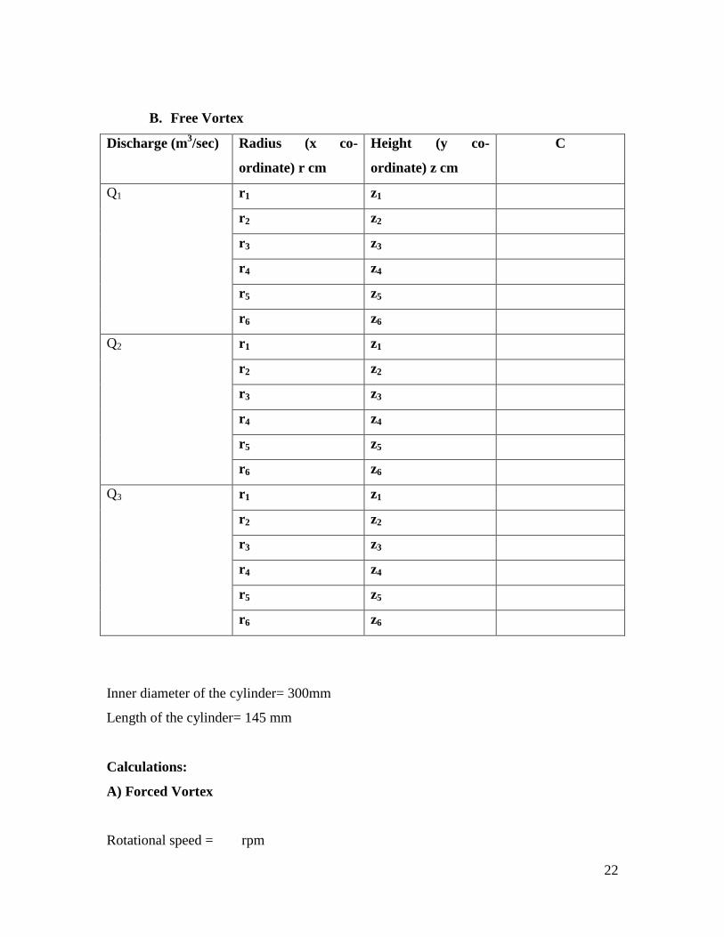
B. Free Vortex

Discharge (m3/sec) Radius (x co-

ordinate) r cm

Height (y co-

ordinate) z cm

C

Q1 r1 z1

r2 z2

r3 z3

r4 z4

r5 z5

r6 z6

Q2 r1 z1

r2 z2

r3 z3

r4 z4

r5 z5

r6 z6

Q3 r1 z1

r2 z2

r3 z3

r4 z4

r5 z5

r6 z6

Inner diameter of the cylinder= 300mm

Length of the cylinder= 145 mm

Calculations:

A) Forced Vortex

Rotational speed = rpm

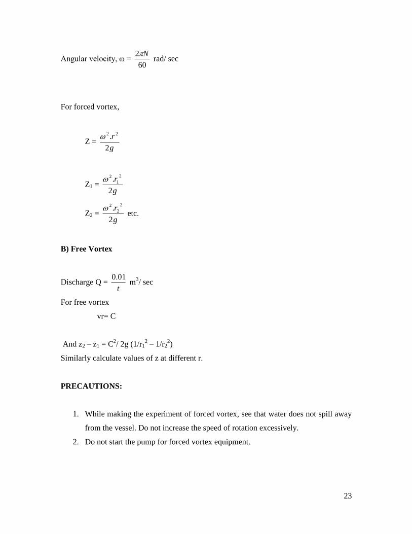
23

Angular velocity, ω = 60

2 N rad/ sec

For forced vortex,

Z = g

r

2

. 22

Z1 = g

r

2

.2

1

2

Z2 = g

r

2

.2

2

2 etc.

B) Free Vortex

Discharge Q = t

01.0 m

3/ sec

For free vortex

vr= C

And z2 – z1 = C2/ 2g (1/r1

2 – 1/r2

2)

Similarly calculate values of z at different r.

PRECAUTIONS:

1. While making the experiment of forced vortex, see that water does not spill away

from the vessel. Do not increase the speed of rotation excessively.

2. Do not start the pump for forced vortex equipment.

24

Experiment No. 08

FLOW ANALYSIS USING REYNOLD’S NUMBER

Aim

Study of different types of flow using Reynold‟s apparatus

Apparatus

TecQuipment H215 Reynolds number and Transitional Flow Demonstration Flow

Apparatus

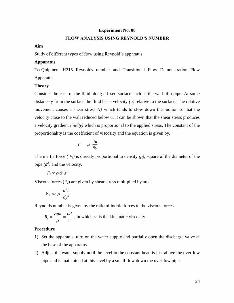
Theory

Consider the case of the fluid along a fixed surface such as the wall of a pipe. At some

distance y from the surface the fluid has a velocity (u) relative to the surface. The relative

movement causes a shear stress (τ) which tends to slow down the motion so that the

velocity close to the wall reduced below u. It can be shown that the shear stress produces

a velocity gradient (∂u/∂y) which is proportional to the applied stress. The constant of the

proportionality is the coefficient of viscosity and the equation is given by,

u

y

The inertia force ( Fi) is directly proportional to density (р), square of the diameter of the

pipe (d2) and the velocity.

Fi ∞2 2 d u

Viscous forces (Fv) are given by shear stress multiplied by area,

Fv ∞2

2

d u

dy

Reynolds number is given by the ratio of inertia forces to the viscous forces

e

ud udR

, in which is the kinematic viscosity.

Procedure

1) Set the apparatus, turn on the water supply and partially open the discharge valve at

the base of the apparatus.

2) Adjust the water supply until the level in the constant head is just above the overflow

pipe and is maintained at this level by a small flow down the overflow pipe.

25

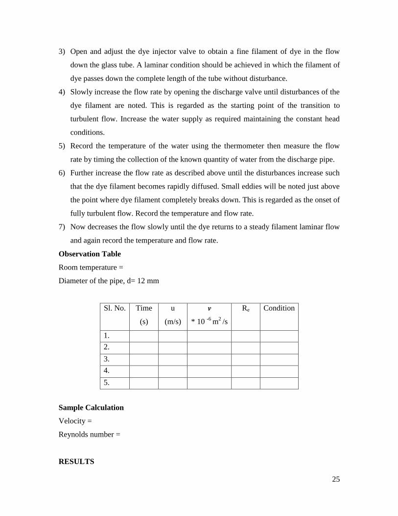
3) Open and adjust the dye injector valve to obtain a fine filament of dye in the flow

down the glass tube. A laminar condition should be achieved in which the filament of

dye passes down the complete length of the tube without disturbance.

4) Slowly increase the flow rate by opening the discharge valve until disturbances of the

dye filament are noted. This is regarded as the starting point of the transition to

turbulent flow. Increase the water supply as required maintaining the constant head

conditions.

5) Record the temperature of the water using the thermometer then measure the flow

rate by timing the collection of the known quantity of water from the discharge pipe.

6) Further increase the flow rate as described above until the disturbances increase such

that the dye filament becomes rapidly diffused. Small eddies will be noted just above

the point where dye filament completely breaks down. This is regarded as the onset of

fully turbulent flow. Record the temperature and flow rate.

7) Now decreases the flow slowly until the dye returns to a steady filament laminar flow

and again record the temperature and flow rate.

Observation Table

Room temperature =

Diameter of the pipe, d= 12 mm

Sl. No. Time

(s)

u

(m/s)

ν

* 10 -6

m2

/s

Re Condition

1.

2.

3.

4.

5.

Sample Calculation

Velocity =

Reynolds number =

RESULTS

26

Experiment No. 09

VENTURIMETER

Aim: To determine the coefficient of discharge of liquid flowing through venturimeter

Apparatus: Venturimeter, Stop watch, Collecting tank, Differential U-tube manometer,

scale etc.

Description:

Venturimeter is a device consisting of a short length of gradual convergence and a long

length of gradual divergence. Pressure tapping is provided at the location before the

convergence commences and another pressure tapping is provided at the throat section of

a Venturimeter. The difference in pressure head between the two tapping is measured by

means of a U-tube manometer. On applying the Continuity equation & Bernoulli‟s

equation between the two sections, the following relationship is obtained in terms of

governing variables.

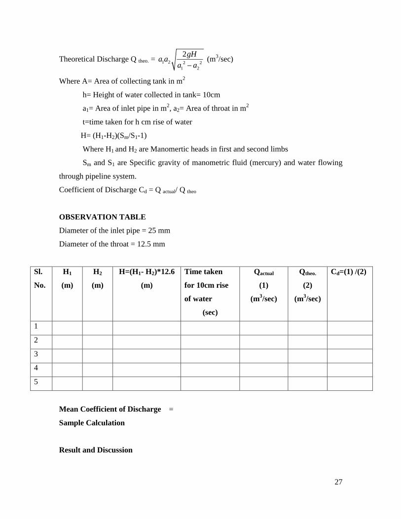
Theoretical Discharge Q theo. = 1 2 2 2

1 2

2gHa a

a a (m

3/sec)

Where, H= (H1-H2)(Sm/S1-1)

Sm and S1 are Specific gravity of manometric fluid (mercury) and water flowing through

pipeline system.

a1= Area of inlet pipe in m2

& a2= Area of throat in m2

Procedure:

The pipe is selected for conducting experiment.

The motor is switched on; as a result water flows through pipes.

The readings of H1and H2 are noted.

The time taken for 10cm rise of water in collecting tank is noted.

The experiment is repeated for different discharges in the same pipe.

Coefficient of Discharge is calculated

Observations:

Volume of Collecting tank (Ah) =30 cm (L) * 30cm (W) * 10cm (h) =

a1= Area of inlet pipe in m2 = a2= Area of throat in m

2 =

Actual Discharge: Q actual = Ah/t (m3/sec)

27

Theoretical Discharge Q theo. = 1 2 2 2

1 2

2gHa a

a a (m

3/sec)

Where A= Area of collecting tank in m2

h= Height of water collected in tank= 10cm

a1= Area of inlet pipe in m2, a2= Area of throat in m

2

t=time taken for h cm rise of water

H= (H1-H2)(Sm/S1-1)

Where H1 and H2 are Manomertic heads in first and second limbs

Sm and S1 are Specific gravity of manometric fluid (mercury) and water flowing

through pipeline system.

Coefficient of Discharge Cd = Q actual/ Q theo

OBSERVATION TABLE

Diameter of the inlet pipe = 25 mm

Diameter of the throat = 12.5 mm

Sl.

No.

H1

(m)

H2

(m)

H=(H1- H2)*12.6

(m)

Time taken

for 10cm rise

of water

(sec)

Qactual

(1)

(m3/sec)

Qtheo.

(2)

(m3/sec)

Cd=(1) /(2)

1

2

3

4

5

Mean Coefficient of Discharge =

Sample Calculation

Result and Discussion

28

Experiment No. 10

LOSSES IN PIPE FITTINGS

AIM: To determine different losses in pipe fittings.

OBJECTIVE: It comprises of the following items.

1. Test set up of the following

2. Stop watch

3. Accessories

INTRODUCTION AND THEORY:

a. Loss of head due to sudden enlargement:-

Consider a liquid flowing through a pipe. Due to sudden enlargement in

diameter from d1 to d2, the liquid flowing from smaller pipe is not able to follow the

sudden change of boundary and turbulent eddies are generated as shown in the figure

resulting in loss of head.

This head loss due to sudden enlargement is given by he= (V1 – V2)2/2g

b. Loss of head due to sudden contraction:-

29

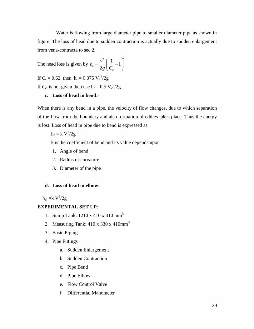
Water is flowing from large diameter pipe to smaller diameter pipe as shown in

figure. The loss of head due to sudden contraction is actually due to sudden enlargement

from vena-contracta to sec.2.

The head loss is given by

22 1

12

c

c

vh

g C

If Cc = 0.62 then hc = 0.375 V22/2g

If Cc is not given then use hc = 0.5 V22/2g

c. Loss of head in bend:-

When there is any bend in a pipe, the velocity of flow changes, due to which separation

of the flow from the boundary and also formation of eddies takes place. Thus the energy

is lost. Loss of head in pipe due to bend is expressed as

hb = k V2/2g

k is the coefficient of bend and its value depends upon

1. Angle of bend

2. Radius of curvature

3. Diameter of the pipe

d. Loss of head in elbow:-

hel =k V2/2g

EXPERIMENTAL SET UP:

1. Sump Tank: 1210 x 410 x 410 mm3

2. Measuring Tank: 410 x 330 x 410mm3

3. Basic Piping

4. Pipe Fittings

a. Sudden Enlargement

b. Sudden Contraction

c. Pipe Bend

d. Pipe Elbow

e. Flow Control Valve

f. Differential Manometer

30

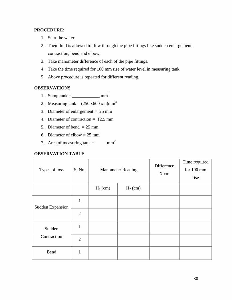
PROCEDURE:

1. Start the water.

2. Then fluid is allowed to flow through the pipe fittings like sudden enlargement,

contraction, bend and elbow.

3. Take manometer difference of each of the pipe fittings.

4. Take the time required for 100 mm rise of water level in measuring tank

5. Above procedure is repeated for different reading.

OBSERVATIONS

1. Sump tank = ____________ mm3

2. Measuring tank = (250 x600 x h)mm3

3. Diameter of enlargement = 25 mm

4. Diameter of contraction = 12.5 mm

5. Diameter of bend = 25 mm

6. Diameter of elbow = 25 mm

7. Area of measuring tank = mm2

OBSERVATION TABLE

Types of loss S. No. Manometer Reading Difference

X cm

Time required

for 100 mm

rise

H1 (cm) H2 (cm)

Sudden Expansion

1

2

Sudden

Contraction

1

2

Bend 1

31

2

Elbow

1

2

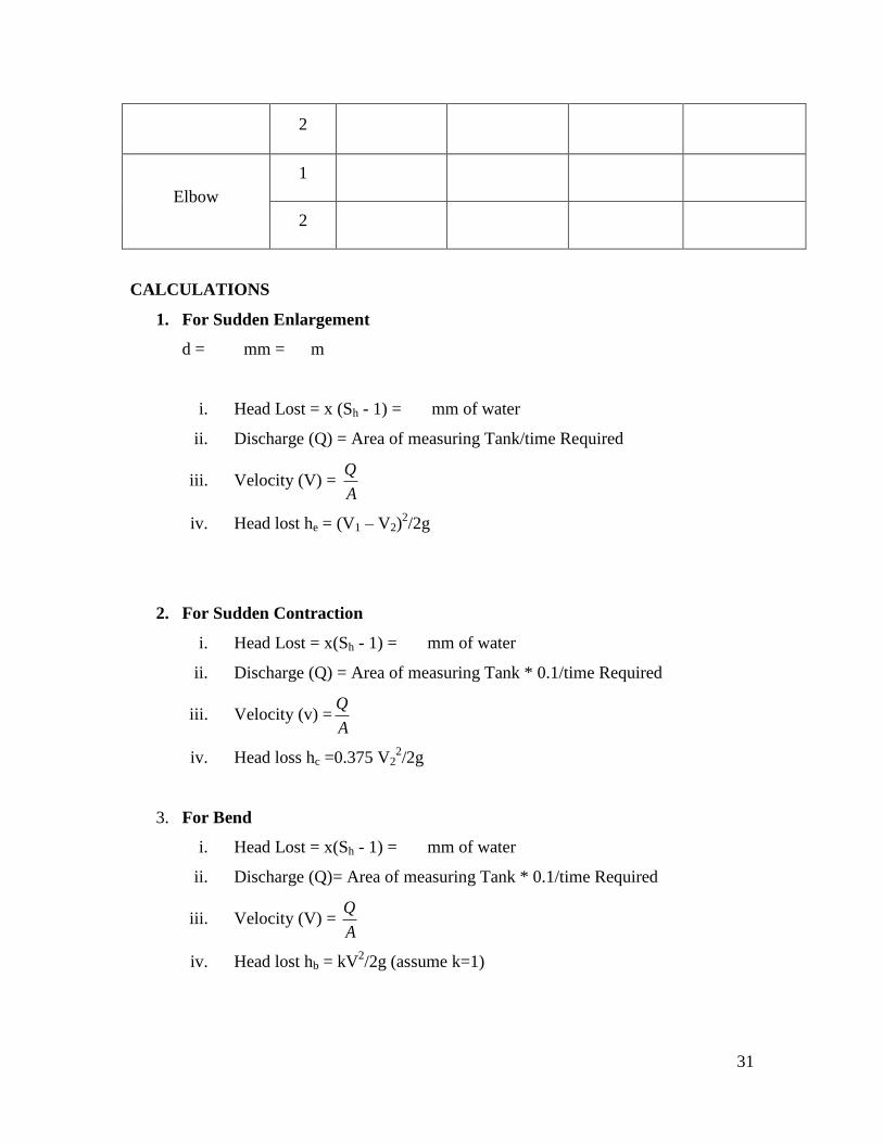
CALCULATIONS

1. For Sudden Enlargement

d = mm = m

i. Head Lost = x (Sh - 1) = mm of water

ii. Discharge (Q) = Area of measuring Tank/time Required

iii. Velocity (V) = Q

A

iv. Head lost he = (V1 – V2)2/2g

2. For Sudden Contraction

i. Head Lost = x(Sh - 1) = mm of water

ii. Discharge (Q) = Area of measuring Tank * 0.1/time Required

iii. Velocity (v) =Q

A

iv. Head loss hc =0.375 V22/2g

3. For Bend

i. Head Lost = x(Sh - 1) = mm of water

ii. Discharge (Q)= Area of measuring Tank * 0.1/time Required

iii. Velocity (V) = Q

A

iv. Head lost hb = kV2/2g (assume k=1)

32

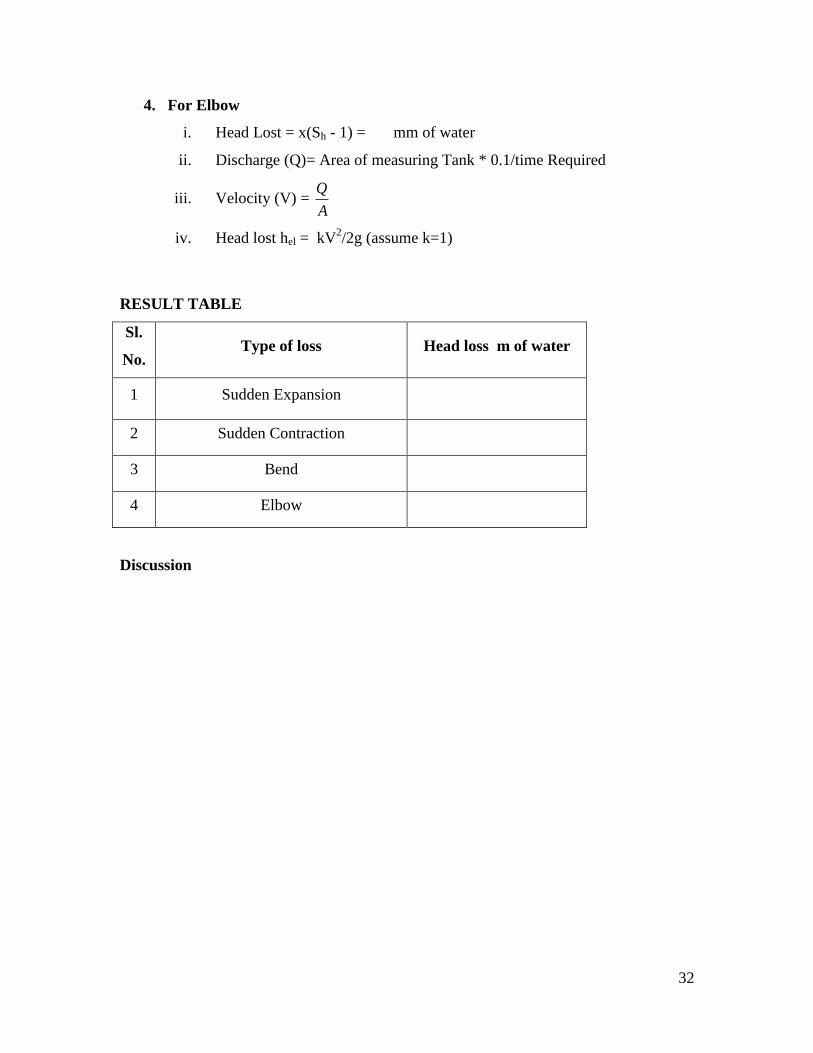
4. For Elbow

i. Head Lost = x(Sh - 1) = mm of water

ii. Discharge (Q)= Area of measuring Tank * 0.1/time Required

iii. Velocity (V) = Q

A

iv. Head lost hel = kV2/2g (assume k=1)

RESULT TABLE

Sl.

No. Type of loss Head loss m of water

1 Sudden Expansion

2 Sudden Contraction

3 Bend

4 Elbow

Discussion

33

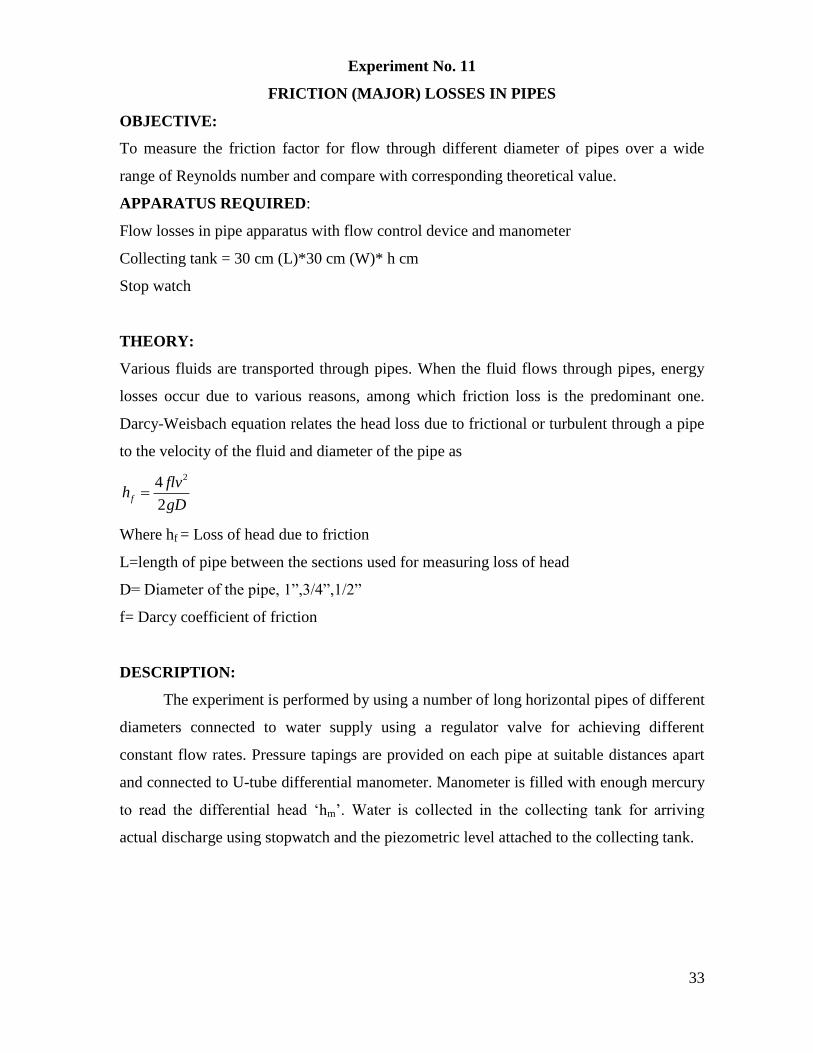
Experiment No. 11

FRICTION (MAJOR) LOSSES IN PIPES

OBJECTIVE:

To measure the friction factor for flow through different diameter of pipes over a wide

range of Reynolds number and compare with corresponding theoretical value.

APPARATUS REQUIRED:

Flow losses in pipe apparatus with flow control device and manometer

Collecting tank = 30 cm (L)*30 cm (W)* h cm

Stop watch

THEORY:

Various fluids are transported through pipes. When the fluid flows through pipes, energy

losses occur due to various reasons, among which friction loss is the predominant one.

Darcy-Weisbach equation relates the head loss due to frictional or turbulent through a pipe

to the velocity of the fluid and diameter of the pipe as

24

2f

flvh

gD

Where hf = Loss of head due to friction

L=length of pipe between the sections used for measuring loss of head

D= Diameter of the pipe, 1”,3/4”,1/2”

f= Darcy coefficient of friction

DESCRIPTION:

The experiment is performed by using a number of long horizontal pipes of different

diameters connected to water supply using a regulator valve for achieving different

constant flow rates. Pressure tapings are provided on each pipe at suitable distances apart

and connected to U-tube differential manometer. Manometer is filled with enough mercury

to read the differential head „hm‟. Water is collected in the collecting tank for arriving

actual discharge using stopwatch and the piezometric level attached to the collecting tank.

34

FORMULAE USED:

1). Darcy coefficient of friction (Friction factor)

2

2

4

fgDhf

Lv

Where * 1mf mh h

hm is differential level of manometer fluid measured in meters)

Qact =Actual discharge measured from volumetric technique.

2).Reynolds number 1D

vDRe

where is the coefficient of dynamic viscosity of

flowing fluid. The viscosity of water is 8.90*10-4

Pa-s at 250 C. Viscosity of water at

different temp is listed below:

Temperature(0C) 10 20 30 40 50 60 70 80 90 100

Viscosity ()

Pa-s *10-4

13.08 10.03 7.978 6.531 5.471 4.668 4.044 3.550 3.150 2.822

PROCEDURE:

1. Note the pipe diameter „D‟, the density of the manometer fluid(mercury) „ m‟

=13600 kg/m3 and the flowing fluid(water) „ ‟=1000 kg/m

3.

2. Make sure only required water regulator valve and required valves at tapings

connected to manometer are opened.

3. Start the pump and adjust the control valve to make pipe full laminar flow. Wait for

some time so that flow is stabilized.

4. Measure the pressure difference „hm‟ across the orifice meter.

5. Note the piezometric reading „Z0‟ in the collecting tank while switch on the

stopwatch.

6. Record the time taken „T‟ and the piezometric reading „Z1‟ in the collecting tank

after allowing sufficient quantity of water in the collecting tank.

7. Increase the flow rate by regulating the control valve and wait till flow is steady.

8. Repeat the steps 4 to 6 for different flows.

RESULTS AND DSICUSSION

35

OBSERVATION AND COMPUTATION-II DATE: _____________________

A) FOR PIPE NO. 1:

Diameter of pipe „D‟= 0.0254 m Area of pipe „A‟= m2 Length of Pipe „L‟= 1 m

Area of collecting tank Act= 0.09 m2 Coefficient of dynamic viscosity at

0C= Pa.s.

Density of the manometer liquid m= 13.6 x 1000 kg/m3 Density of the flowing liquid = 1000 kg/m

3

Tabulation 5.1- For pipe No. 1.

No. Actual Measurement Calculated values f Re No. Log (Re)

Time T

(sec)

Z1(m) Z0(m) hm(m) Collecting tank

hct(m) (3)-(4)

Volume(m3) Act*hct

Discharge Qact

(7)/(2)

Velocity (8)/A

hf(m)

(5)* 1m

2

2

4

fgDhf

Lv vD

(1) (2) (3) (4) (5) (6) (7) (8) (9) (10) (11) (12) (13)

1

2

3

4

5

6

7

8

9

10

36

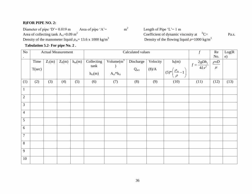
B)FOR PIPE NO. 2:

Diameter of pipe „D‟= 0.019 m Area of pipe „A‟= m2 Length of Pipe „L‟= 1 m

Area of collecting tank Act=0.09 m2 Coefficient of dynamic viscosity at

0C= Pa.s.

Density of the manometer liquid m= 13.6 x 1000 kg/m3 Density of the flowing liquid =1000 kg/m

3

Tabulation 5.2- For pipe No. 2 .

No

.

Actual Measurement Calculated values f Re

No.

Log(R

e)

Time

T(sec)

Z1(m) Z0(m) hm(m) Collecting

tank

hct(m)

(3)-(4)

Volume(m3

)

Act*hct

Discharge

Qact

(7)/(2)

Velocity

(8)/A

hf(m)

(5)* 1m

2

2

4

fgDhf

Lv

vD

(1) (2) (3) (4) (5) (6) (7) (8) (9) (10) (11) (12) (13)

1

2

3

4

5

6

7

8

9

10

37

C)FOR PIPE NO. 3:

Diameter of pipe „D‟= 0.0127 m Area of pipe „A‟= m2 Length of Pipe „L‟= 1 m

Area of collecting tank Act= 0.09 m2 Coefficient of dynamic viscosity at

0C= Pa.s.

Density of the manometer liquid m = 13.6 x 1000 kg/m3 Density of the flowing liquid =1000 kg/m

3

Tabulation 5.3- For pipe No. 3 .

Sl.

No

.

Actual Measurement Calculated values f Re

No.

Log

(Re)

Time

T(sec)

Z1(m) Z0(m) hm(m) Collecting

tank

hct(m)

(3)-(4)

Volume(m3)

Act*hct

Discharge

Qact

(7)/(2)

Velocit

y

(8)/A

hf(m)

(5)* 1m

2

2

4

fgDhf

Lv

vD

(1) (2) (3) (4) (5) (6) (7) (8) (9) (10) (11) (12) (13)

1

2

3

4

5

6

7

8

9

10

38

Experiment No. 12

ORIFICE METER

Aim: To determine the coefficient of discharge of orifice meter.

Apparatus: Orifice meter, Stop watch, Collecting tank, Differential U-tube manometer.

Description:

Orifice meter is a device used for measuring the rate of flow of a fluid through a pipe.

Orificemeter works on the same principle as that of Venturimeter i.e. by reducing the area

of flow passage a pressure difference is developed between the two sections and the

measurement of pressure difference is used to find the discharge.

It consists of a flat circular plate which has a circular sharp edge hole called orifice,

which is concentric with the pipe. The orifice diameter is kept generally 0.5 times the

diameter of the pipe, though it may vary from 0.4 to 0.8 times the pipe diameter.

A mercury U-tube manometer is connected at section (1), which is at a distance of about

1.5 to 2.0 times the pipe diameter upstream from the orifice plate, and at section (2)

which is at a distance of about half the diameter of the orifice on the downstream side

from the orifice plate to know the pressure head between the two tappings.

Procedure:

The pipe is selected for conducting experiment.

The motor is switched on; as a result water flows through pipes.

The readings of H1and H2 are noted.

The time taken for 10cm rise of water in collecting tank is noted.

The experiment is repeated for different discharges in the same pipe.

Coefficient of Discharge is calculated

Formulae

Actual Discharge: Q actual = Ah/t (m3/sec)

Theoretical Discharge Q theo. = 1 2 2 2

1 2

2gHa a

a a (m

3/sec)

Where A= Area of collecting tank in m2

39

h= Height of water collected in tank = 10cm

a1= Area of inlet pipe in m2

a2= Area of throat in m2

t=time taken for h cm rise of water

H= (H1-H2)(Sm/S1-1)

Where H1 and H2 are Manomertic heads in first and second limbs

Sm and S1 are Specific gravity of manometric fluid (mercury) and water flowing through

the pipeline system.

Density of the manometer liquid m= 13.6 x 1000 kg/m3

Density of the flowing liquid = 1000 kg/m3

Coefficient of Discharge Cd = Q actual/ Q theo

Volume of Collecting tank (Ah) =30cm (L) * 30cm (W) * 10cm (h) =

Diameter of the inlet pipe = 25 mm

Diameter of the throat = 12.5 mm

a1= Area of inlet pipe in m2 =

a2= Area of throat in m2

=

OBSERVATION TABLE

Sl.

No.

H1

(m)

H2

(m)

H=(H1H2)*12.6

(m)

Time taken for

10cm rise of water

(sec)

Qactual

(1)

Qtheo.

(2)

Cd=

(1)/(2)

1

2

3

4

5

6

Mean Coefficient of Discharge =

Sample Calculation

Result and Discussion