Gutenberg School of Management and Economics 

Discussion Paper Series

Existence, Uniqueness and Stability of Invariant Distributions in Continuous-Time

Stochastic Models  

Christian Bayer and Klaus Wälde

July 2011

Discussion paper number 1111

Johannes Gutenberg University Mainz Gutenberg School of Management and Economics

Jakob-Welder-Weg 9 55128 Mainz

Germany wiwi.uni-mainz.de

Contact details

Christian Bayer Department of Mathematics University of Vienna Nordbergstrasse 15 1090 Wien Austria

christian.bayer@univie.ac.at

Klaus Wälde Chair in Macroeconomics Johannes Gutenberg-Universität Mainz Jakob Welder-Weg 4 55128 Mainz Germany klaus.waelde@uni-mainz.de

All discussion papers can be downloaded from http://wiwi.uni-mainz.de/DP 

Existence, Uniqueness and Stabilityof Invariant Distributions

in Continuous-Time Stochastic Models

Christian Bayer(a) and Klaus Wälde(b)(a) University of Vienna and

(b) University of Mainz, CESifo and Université catholique de Louvain1

July 2011

We study a dynamic stochastic general equilibrium model in continuoustime. Related work has proven that optimal consumption in this modelis a smooth function of state variables. This allows us to describe theevolution of optimal state variables (wealth and labour market status) bystochastic di¤erential equations. We derive conditions under which aninvariant distribution for state variables exists and is unique. We alsoprovide conditions such that initial distributions converge to the long-rundistribution.

JEL Codes: C62, D91, E24, J63Keywords: uncertainty in continuous time, Poisson process,

existence, uniqueness, stability

1 Introduction

Dynamic stochastic general equilibrium models are widely used for macro economicanalysis and also for many analyses in labour economics. When the developmentof these models started with the formulation of stochastic growth models, a lot ofemphasis was put on understanding formal properties of these models. Does a uniquesolution exist, both for the control variables and general equilibrium itself? Is there astationary long-run distribution (of state variables being driven by optimally chosencontrol variables) to which initial distributions of states converge? This literatureis well developed for discrete time models (see below for a short overview). Whenit comes to continuous time models, however, only initially there were some articleslooking at stability issues (Merton, 1975; Bismut, 1975; Magill, 1977; Brock andMagill, 1979; Chang and Malliaris, 1987). In recent decades, applications to economicquestions have been the main focus. This does not mean, however, that all formalproblems have been solved. In fact, we argue in this paper that formal work is badly

1Christian Bayer: University of Vienna, Department of Mathematics, Nordbergstrasse 15, 1090Wien, Austria, christian.bayer@univie.ac.at. Klaus Wälde: University of Mainz, Gutenberg Schoolof Management and Economics, Jakob-Welder-Weg 4, 55128 Mainz, Germany. klaus@waelde.com,www.waelde.com. We are grateful to William Brock, John Stachurski and Stephen Turnovsky forcomments and suggestions.

1

missing for continuous time uncertainty which has strong implications for appliedwork.An area in economics where continuous-time stochastic models are especially pop-

ular is the labour-market search and matching literature. While all of these modelsare dynamic and stochastic by their basic structure (new job opportunities arise atrandom points in time only and/or new wage o¤ers are random), there has been verylittle e¤ort in understanding the stability properties of their distributional predic-tions.2 This might be due to two reasons. Some papers work with a law of largenumbers right from the beginning which allows to focus on means. The classic ex-ample is Pissarides (1985). Papers in the tradition of Burdett and Mortensen (1998)that do focus on distributions construct these distributions by focusing on �steadystates�, i.e. on distributions which are time-invariant.3

While this approach is extremely fruitful to understand a lot of important issues,one might also want to understand how distributions evolve over time.4 Once thisbecomes the objective, the issue of stability and uniqueness of a long-run stationarydistribution becomes central.The goal of this paper is threefold: First, we introduce methods for analysing exis-

tence and stability of distributions described by stochastic di¤erential equations fromthe mathematical literature. The approach to proving the existence and uniquenessof an invariant distribution and its ergodicity, i.e. of convergence to the said distrib-ution, builds on the work of Meyn and Tweedie (1993 a,b,c) and Down et al. (1995).Their work is especially useful for understanding properties of systems driven by jumpprocesses.5 The methods we use here would be the ones that can be applied to thesearch and matching analyses cited above.Second, we use these methods to analyse stability properties of a model of search

and matching where individuals can smooth consumption by accumulating wealth.The model was originally developed and analyzed in a companion paper (Bayer andWälde, 2011). Individuals have constant relative risk aversion and an in�nite planninghorizon.6 Optimal behaviour implies that the two state variables of an individual,wealth and employment status, follow a process described by two stochastic di¤er-ential equations. We analyse under which conditions a distribution for wealth andemployment status exists, is unique and converges to an invariant long-run distribu-

2The literature on assortative matching carefully analyses existence and uniqueness issues (see e.g.Shimer and Smith, 2000 or Lentz, 2010). These analyses do not take the dynamics of distributionsinto account.

3Papers in this tradition include Postel-Vinay and Robin (2002), Cahuc et al. (2006), Moscarini(2005) and Burdett et al. (2011), to name just a few.

4There is a very recent strand of the literature which inquires into the evolution of distribu-tions over the business cycle. Examples include Moscarini and Postel-Vinay (2008, 2010), Colesand Mortensen (2011) and Kaas and Kircher (2011). These papers all analyse the evolution ofdistributions over time.

5These methods are also used for understanding how to estimate models that contain jumps(e.g. Bandi and Nguyen, 2003) or for understanding long-term risk-return trade-o¤s (Hansen andScheinkman, 2009).

6See related work by Alvarez and Shimer (2011) who allow for risk-sharing within large house-holds, endogenous labour supply and a di¤erentiated production structure. They do not include asavings decision.

2

tion. The corresponding theorem is proven.Our third objective consists in illustrating the usefulness of the methods presented

here for other stochastic continuous-time models. The examples we have in mind (seebelow) mainly come from macro, labour, �nance and international �nance. Illus-trating how these methods can be applied in other contexts should make it easy todevelop some intuition for understanding which models with evolving distributionspredict stability.One crucial component of our proofs is a smoothing condition. As we allow for

Poisson processes, we have to use more advanced methods based on T -processes thanin the case of a stochastic di¤erential equation driven by a Brownian motion. Inthe latter case the strong smoothing properties of Brownian motion can be used toobtain the strong Feller property. In this sense, the corresponding analysis will oftenbe more straightforward than the one presented here. For the wealth-employmentprocess of Bayer and Wälde, we �nd that the wealth process is not smoothing andthe strong Feller property does not hold. However, for the economically relevantparameter case (the low-interest rate regime), we can still show a strong version ofrecurrence (namely Harris recurrence) by using a weaker smoothing property, andthus obtain uniqueness of the invariant distribution. Ergodicity is then implied byproperties of discrete skeleton chains.Let us relate our approach to the more formal literature. In discrete time models,

a classic analysis was undertaken by Brock and Mirman (1972). They analyse anin�nite-horizon optimal stochastic growth model with discounting where uncertaintyresults from total factor productivity. They show inter alia that �the sequence ofdistribution functions of the optimal capital stocks converges to a unique limitingdistribution.� Methodologically, they use parts of the classical stability theory ofMarkov chains, but mainly rely on properties of their model. A nice presentation ofstability theory for Markov processes with a general state space is by Futia (1982). Heuses an operator-theoretic approach exploiting results from the theory of continuouslinear operators on Banach spaces. Hopenhayn and Prescott (1992) analyse existenceand stability of invariant distributions exploiting monotonicity of decision rules thatresult from optimal behaviour of individuals. Their approach mainly relies on �xedpoint theorems for increasing maps and increasing operators on measures (in the senseof stochastic dominance). Bhattacharya and Majumdar (2004) provide an overview ofresults concerning the stability of random dynamic systems with a brief application tostochastic growth. Nishimura and Stachurski (2005) present a stability analysis basedon the Foster�Lyapunov theory of Markov chains. For a survey of stochastic optimalgrowth models, see Olson and Roy (2006). In the literature on precautionary savings,Huggett (1993) analyses an exchange economy with idiosyncratic risk and incompletemarkets. Agents can smooth consumption by holding an asset and endowment in eachperiod is either high or low, following a stationary Markov process. This structureis similar in spirit to our setup. Huggett provides existence and uniqueness resultsfor the value function and the optimal consumption function and shows that thereis a unique long-run distribution function to which initial distributions converge.Regarding stability, he relies on the results of Hopenhayn and Prescott (1992).The theory we will employ below provides a useful contribution to the economic

3

literature as the latter, as just presented, focuses on related, but di¤erent methods.For one, we treat Markov processes in continuous time, while references in the macro-economic literature in the context of Markov-process stability are mostly related todiscrete time.7 But even in discrete time, the theory of Meyn and Tweedie andtheir coauthors di¤ers from the approaches cited above. Indeed, Meyn and Tweedie�stheory is a direct generalization of the classical stability theory for Markov chains indiscrete time, with �nite, discrete state space.In the economic continuous�time literature, the starting point is Merton�s (1975)

analysis of the continuous-time stochastic growth model. For the case of a constantsaving rate and a Cobb-Douglas production function, the �steady-state distributionsfor all economic variables can be solved for in closed form�. No such closed formresults are available of course for the general case of optimal consumption. Changand Malliaris (1987) also allow for uncertainty that results from stochastic populationgrowth as in Merton (1975) and they assume the same exogenous saving functionwhere savings are a function of the capital stock. They follow a di¤erent route,however, by studying the class of strictly concave production functions (thus includingCES production function and not restricting their attention to the Cobb-Douglascase). They prove �existence and uniqueness of the solution to the stochastic Solowequation�. The build their proof on the so-called Re�ection Principle. More workon growth was undertaken by Brock and Magill (1979) building on Bismut (1975).Magill (1977) undertakes a local stability analysis for a many-sector stochastic growthmodel with Brownian motions using methods going back to Rishel (1970). All ofthese models use Brownian motion as their source of uncertainty and do not allowfor Poisson jumps. To the best of our knowledge, not much (no) work has been doneon these issues since then.The structure of our paper is as follows. The next section presents the model.

Section 3 introduces the mathematical background for our existence and stabilityanalysis. We remind the reader of familiar results from discrete-time stability analysisand then introduce corresponding concepts in continuous time. Section 4 appliesthese methods to our model and proves existence and uniqueness of an invariantmeasure for the process describing the state variables. Section 4 also proves thatinitial conditions converge to the long-run invariant distribution. Section 5 appliesour methods to three stochastic processes originating from a long list of other papersin the literature. Section 6 concludes.

2 The model

Consider an individual that maximizes a standard intertemporal utility function,U (t) = Et

R1te��[��t]u (c (�)) d�; where expectations need to be formed due to the

uncertainty of labour income which in turn makes consumption c (�) uncertain. Theexpectations operator is Et and conditions on the current state in t: The planninghorizon starts in t and is in�nite. The time preference rate � is positive. We assume

7As already remarked earlier, continuous time models are treated thoroughly, but under di¤erentconditions, in the �nance literature.

4

that the instantaneous utility functions has a CRRA structure u (c (�)) = c(�)1���11��

with � 6= 1: All proofs for the logarithmic case � = 1 should work accordingly.Each individual can save in an asset a. Her budget constraint reads

da (t) = fra (t) + z (t)� c (t)g dt: (1)

Per unit of time dt wealth a (t) increases (or decreases) if capital income ra (t) pluslabour income z (t) is larger (or smaller) than consumption c (t) : Labour incomez (t) is given either by constants w or b8 and is intuitively described by the secondconstraint of the household, a stochastic di¤erential equation,

dz (t) = �dq� ��dqs; � � w � b: (2)

The Poisson process qs counts how often our individual moves from employment intounemployment. The arrival rate of this process is given by s > 0 when the individualis employed and by s = 0 when the individual is unemployed. The Poisson processrelated to job �nding is denoted by q� with an arrival rate � > 0 when unemployedand � = 0 when employed (as there is no search on the job). It counts how oftenthe individual �nds a job. In e¤ect, z(t) is a continuous time Markov chain withstate space fw; bg, where the transition w ! b happens with rate s and the transitionb! w with rate �. This description of z will be used in the remainder of the paper.As usual, the wealth-employment process (a; z), is de�ned on a probability space(;F ; P ).When we allow the individual to optimally choose the consumption level c (t) ;

we make the following assumptions (see Bayer and Wälde, 2011 for details): (i) Theinterest rate is lower than the time-preference rate, r < �, (ii) optimal consumptionc (a; z) is continuously di¤erentiable on [�b=r; a�w] � fw; bg in a, (iii) relative con-sumption c(a; w)=c(a; b) is continuously di¤erentiable in a and the derivative changesits sign only �nitely often in every �nite interval and (iv) the initial wealth a(t) ischosen inside the interval [�b=r; a�w]. The discussion in Bayer and Wälde (2011, seethe phase diagram there for an illustration) has revealed that wealth a(�) 2]�b=r; a�w[is increasing when z(�) = w and decreasing when z(�) = b. Moreover, wealth willnever leave the interval [�b=r; a�w].

3 Ergodicity results for continuous time Markovprocesses

The wealth-employment process (a(�); z(�)) is a continuous-time Markov process witha non-discrete state space [�b=r; a�w]� fw; bg. Thus, we will rely on results from thegeneral stability theory of Markov processes as presented in the works of Meyn andTweedie and their coauthors cited above. In the present section, we will recapitulate

8In the full model of Bayer and Wälde (2011), w and b are endogenous functions of the equilib-rium capital stock. This is of no importance for the distributional analysis here and we thereforeimmediately assume w > b and b to be constant.

5

the most important elements of the stability for Markov processes in continuous time.Here, we will discuss the theory in full generality, i.e., we assume that we are given aMarkov process (Xt)t2R�0 on a state spaceX, which is assumed to be a locally compactseparable metric space endowed with its Borel �-algebra. All Markov processes areassumed to be time-homogeneous, i.e., the conditional distribution of Xt+s givenXt = x only depends on s, not on t.

3.1 Preliminaries

Let (Xt)t2R�0 be a (homogeneous) Markov process with the state space X, where Xis assumed to be a locally compact and separable metric space, which is endowedwith its Borel �-algebra B(X). Let P t(x;A), t � 0, x 2 X, A 2 B(X), denote thecorresponding transition kernel, i.e.

P t(x;A) � P (Xt 2 AjX0 = x) � Px(Xt 2 A); (3)

where Px is a shorthand-notation for the conditional probability P (�jX0 = x). Notethat P t(�; �) is a Markov kernel, i.e. for every x 2 X, the map A 7! P t(x;A) is a prob-ability measure on B(X) and for every A 2 B(X), the map x 7! P t(x;A) is a measur-able function. Similarly, by a kernel we understand a function K : (X;B(X))! R�0such that K(x; �) is a measure, not necessarily normed by 1, for every x and K(�; A)is a measurable function for every measurable set A. Moreover, let us denote thecorresponding semi-group by Pt, i.e.

Ptf(x) � E(f(Xt)jX0 = x) =

ZX

f(y)P t(x; dy) (4)

for f : X! R bounded measurable. For a measurable set A, we consider the stoppingtime �A and the number of visits of X in set A;

�A � infft � 0jXt 2 Ag; �A �Z 1

0

1A(Xt)dt;

De�nition 3.1 Assume that there is a �-�nite, non-trivial measure ' on B(X) suchthat, for sets B 2 B(X), '(B) > 0 implies Ex(�B) > 0, 8x 2 X. Here, similar to Px,Ex is a short-hand notation for the conditional expectation E(�jX0 = x). Then X iscalled '-irreducible.

In the more familiar case of a �nite state space and discrete time, we would simplyrequire �fxg to have positive expectation for any state x. In the continuous case, sucha requirement would obviously be far too strong, since singletons fxg usually haveprobability zero. The above de�nition only requires positive expectation for sets B,which are �large enough�, in the sense that they are non-null for some referencemeasure.A simple su¢ cient condition for irreducibility is given in Meyn and Tweedie

(1993b, prop. 2.1), which will be used to show irreducibility of the wealth-employmentprocess.

6

Proposition 3.2 Suppose that there exists a �-�nite measure � such that �(B) > 0implies that Px(�B <1) > 0. Then X is '-irreducible, where

'(A) �ZX

R(x;A)�(dx); R(x;A) �Z 1

0

P t(x;A)e�tdt:

De�nition 3.3 The process X is called Harris recurrent if there is a non-trivial �-�nite measure ' such that '(A) > 0 implies that Px(�A =1) = 1, 8x 2 X. Moreover,if a Harris recurrent process X has an invariant probability measure, then it is calledpositive Harris.

Like in the discrete case, Harris recurrence may be equivalently de�ned by theexistence of a �-�nite measure � such that �(A) > 0 implies that Px(�A < 1) = 1.As already remarked in the context of irreducibility, in the discrete framework onewould consider sets A = fyg with only one element.Let � be a measure on (X;B(X)). We de�ne a measure P t� by

P t�(A) =

ZX

P t(x;A)�(dx):

We say that � is an invariant measure, i¤P t� = � for all t. Here, the measure � mightbe in�nite. If it is a �nite measure, we may, without loss of generality, normalize itto have total mass �(X) = 1. The resulting probability measure is obviously stillinvariant, and we call it an invariant distribution. (Note that any constant multipleof an invariant measure is again invariant.) In the case of an invariant distribution,we can interpret invariance as meaning that the Markov process has always the samemarginal distribution in time, when starting with the distribution �.

3.2 Existence of an invariant probability measure

The existence of �nite invariant measures follows from a combination of two di¤erenttypes of conditions. The �rst property is a growth property. Several such proper-ties have been used in the literature, a very useful one seems to be boundedness inprobability on average.

De�nition 3.4 The process X is called bounded in probability on average if forevery x 2 X and every � > 0 there is a compact set C � X such that

lim inft!1

1

t

Z t

0

Px(Xs 2 C)ds � 1� �: (5)

The second property is a continuity condition.

De�nition 3.5 The Markov process X has the weak Feller property if for everycontinuous bounded function f : X ! R the function Ptf : X ! R from (4) isagain continuous. Moreover, if Ptf is continuous even for every bounded measurablefunction f , then X has the strong Feller property.

7

Given these two conditions, Meyn and Tweedie (1993b, th. 3.1) establish theexistence of an invariant probability measure in the following

Proposition 3.6 If a Markov process X is bounded in probability on average and hasthe weak Feller property, then there is an invariant probability measure for X.

3.3 Uniqueness

Turning to uniqueness, the following proposition is cited in Meyn and Tweedie (1993b,page 491). For a proof see Azéma, Du�o and Revuz (1969, Théorème 2.5).

Proposition 3.7 If the Markov process X is Harris recurrent and irreducible fora non-trivial �-�nite measure ', then there is a unique invariant measure (up toconstant multiples).

Proposition 3.7 gives existence and uniqueness of the invariant measure. A simpleexample shows that irreducibility and Harris recurrence do not guarantee existence ofan invariant probability measure: LetX = R and Xt = Bt denote the one-dimensionalBrownian motion. The Brownian motion is both irreducible and Harris recurrent �irreducibility is easily seen, while recurrence is classical in dimension one. Therefore,there is a unique invariant measure. By the Fokker-Planck equation, the density f ofthe invariant measure must satisfy �f = 0. By non-negativity, this implies that f isconstant, f � c for some c > 0. Thus, any invariant measure is a constant multiple ofthe Lebesgue measure, and there is no invariant probability measure for this example.Given this example and as we are only interested in invariant probability mea-

sures, we need to combine this proposition with the previous section: Boundedness inprobability on average together with the weak Feller property gives us the existence ofan invariant probability measure as used in sect. 3.2, whereas irreducibility togetherwith Harris recurrence imply uniqueness of invariant measures. Thus, for existenceand uniqueness of the invariant probability measure, we will need all four conditions.Whereas irreducibility, boundedness in probability on average and the weak Feller

property are rather straightforward to check in practical situations, this seems to beharder for Harris recurrence. Thus, we next discuss some su¢ cient conditions forHarris recurrence. If the Markov process has the strong Feller property, then Harrisrecurrence will follow from a very weak growth property, namely that Px(Xt !1) =0 for all x 2 X, see Meyn and Tweedie (1993b, th. 3.2). While the strong Fellerproperty is often satis�ed for models driven by Brownian motion (e.g., for hypo-elliptic di¤usions), it may not be satis�ed in models where randomness is driven bya pure-jump process. Thus, we will next formulate an intermediate notion betweenthe weak and strong Feller properties, which still guarantees enough smoothing forstability.

De�nition 3.8 The Markov process X is called T-process, if there is a probabilitymeasure � on R�0 and a kernel T on (X;B(X)) satisfying the following three condi-tions:

8

1. For every A 2 B(X), the function x 7! T (x;A) is continuous9.

2. For every x 2 X and every A 2 B(X) we have K� (x;A) �R10P t(x;A)�(dt) �

T (x;A).

3. T (x;X) > 0 for every x 2 X.

The kernel K� is the transition kernel of a discrete-time Markov process (Yn)n2Nobtained from (Xt)t�0 by random sampling according to the distribution �: moreprecisely, let us draw a sequence �n of independent samples from the distribution� and de�ne a discrete time process Yn � X�1+���+�n, n 2 N. Then the process Ynis Markov and has transition probabilities given by K� : Using this de�nition andtheorem 3.2 in Meyn and Tweedie (1993b), we can formulate

Proposition 3.9 Suppose that X is a '-irreducible T-process. Then it is Harrisrecurrent (with respect to ') if and only if Px(Xt !1) = 0 for every x 2 X.

Hence, in a practical sense and in order to prove existence of a unique invariantprobability measure, one needs to establish that a process X has the weak Fellerproperty and is an irreducible T -process which is bounded in probability on average(as the latter implies the growth condition Px(Xt !1) = 0 of prop. 3.9).Let us shortly compare the continuous, but compact case �where boundedness

in probability is always satis�ed �with the discrete case. In the latter situation,existence of an invariant distribution always holds, while uniqueness is then given byirreducibility. In the compact, continuous case irreducibility and Harris recurrenceonly guarantee existence and uniqueness of an invariant measure, which might bein�nite. On the other hand, existence of a �nite invariant measure is given by theweak Feller property. Thus, for existence and uniqueness of an invariant probabilitymeasure, we will need the weak Feller property, irreducibility and Harris recurrence�which we will conclude from the T-property. Thus, the situation in the continuous(but compact) case is roughly the same as in the discrete case, except for somerequired continuity property, namely the weak Feller property.

3.4 Stability

By now we have established a framework for showing existence and uniqueness of aninvariant distribution, i.e., probability measure. However, under stability we under-stand more, namely the convergence of the marginal distributions to the invariantdistribution, i.e., that for any starting distribution �, the law P �� of the Markovprocess at time � converges to the unique invariant distribution for � ! 1. In thecontext of T -processes, we are going to discuss two methods which allow to derivestability. But �rst, let us de�ne the notion of stability in a more precise way.

9A more general de�nition requires lower semi-continuity only. As we can show continuity forour applications, we do not need this more general version here.

9

De�nition 3.10 For a signed measure � consider the total variation norm

k�k � supjf j�1

����ZX

f(x)�(dx)

���� :Then we call a Markov process (Xt)t2R�0 stable or ergodic i¤ there is an invariantprobability measure � such that

8x 2 X : limt!1

kP t(x; �)� �k = 0:

Note that this implies in particular that the law P t� of the Markov process con-verges to �, which is the unique invariant probability measure.In the case of a �nite state space in discrete time, ergodicity follows (inter alia)

from aperiodicity. Down, Meyn and Tweedie (1995), also give one continuous resultin this direction.

De�nition 3.11 A -irreducible Markov process (Xt) is called aperiodic i¤ there isa measurable set C with (C) > 0 satisfying the following properties:

1. there is � > 0 and a non-trivial measure � on B(X) such that8x 2 C; 8A 2 B(X) : P � (x;A) � �(A); 10

2. there is T > 0 such that

8t � T; 8x 2 C : P t(x;C) > 0:

If we are given an irreducible, aperiodic Markov process, then stability is impliedby conditions on the in�nitesimal generator. In the following proposition we give aspecial case of Down, Meyn and Tweedie (1995, th. 5.2) suitable for the employment-wealth process in our model.

Proposition 3.12 Given an irreducible, aperiodic T-process Xt with in�nitesimalgenerator A on a compact state space. Assume we can �nd a measurable functionV 2 D(A) with V � 1 and constants d; c > 0 such that

AV � �cV + d:

Then the Markov-process is ergodic.

The problem with aperiodicity in the continuous time framework is that it seemshard to characterize the small sets appearing in def. 3.11. For this reason, we alsogive an alternative theorem, which avoids small sets (but is clearly related with thenotion of aperiodicity). Given a �xed � > 0, the process Yn � X�n, n 2 N, clearlyde�nes a Markov process in discrete time, a so-called skeleton of X. These skeletonchains are a very useful construction for transferring results from Markov processesin discrete time to continuous time. In particular, Meyn and Tweedie (1993b, th. 6.1)gives a characterization of stability in terms of irreducibility of skeleton chains.

Proposition 3.13 Given a Harris recurrent Markov process X with invariant prob-ability measure �. Then X is stable i¤ there is some irreducible skeleton chain.10Such a set C is then called small.

10

4 Stability of the wealth-employment process

Turning to our main application, we would like to understand the stability propertiesof the model developed by Bayer and Wälde (2011). Understanding stability meansunderstanding the dynamic properties of the state variables of the model. All othervariables (like control variables or e.g. factor rewards) are known deterministic func-tions of the state variables. Hence, if we understand the process governing the statevariables, we also understand the properties of all other variables in this model.As the fundamental state variables in Bayer and Wälde (2011) are wealth and the

employment status of an individual, the process we are interested in is the wealth-employment process X� � (a (�) ; z (�)) : The state-space of this process is X �[�b=r; a�w]� fw; bg and has all the properties required for the state space in sect. 3.We now follow the structure of sect. 3.

4.1 Existence

In order to show existence for an invariant probability measure for X, prop. 3.6 tellsus that we need to prove that X is (i) bounded in probability on average and (ii) hasthe weak Feller property. Showing that X is bounded in probability on average isstraightforward: According to def. 3.4 we need to �nd a compact set for any initialcondition x and any small number � such that the average probability to be in thisset is larger than 1� �: As our process X� � (a (�) ; z (�)) is bounded, we can choosethe state-space X � [�b=r; a�w] � fw; bg as our set for any x and �. Concerning theweak Feller property, we o¤er the following

Lemma 4.1 The wealth-employment process has the weak Feller property.

Proof. Let us �rst show that the wealth-employment process depends continu-ously on its initial values. To see this, �x some ! 2 , the probability space, onwhich the wealth-employment process is de�ned. Notice that z� (!) is certainly con-tinuous in the starting values, because any function de�ned on fw; bg is continuousby our choice of topology. Thus, we only need to consider the wealth process. For�xed !, a� (!) is a composition of solutions to deterministic ODEs, each of which arecontinuous functions of the respective initial value. Therefore, a� (!) is a continuousfunction of the initial wealth.Now assume, without loss of generality, that the wealth-employment process has

a deterministic initial value (a0; z0) and �x some bounded, continuous function f :[�b=r; a�w]� fw; bg ! R. For the weak Feller property, we need to show that

P�f(a0; z0) = E (f(a� ; z� ))

is a continuous function in (a0; z0). Thus, take any sequence (an0 ; zn0 ) converging

to (a0; z0) and denote the wealth-employment process started at (an0 ; zn0 ) by (a

n� ; z

n� ).

Then, by continuous dependence on the initial value, (an� (!); zn� (!))! (a� (!); z� (!)),

for every ! 2 . By continuity of f , this implies convergence of f (an� (!); zn� (!)).Since f is bounded, we may conclude convergence P�f (an0 ; z

n0 ) ! P�f(a0; z0) by

11

the dominated convergence theorem. So, P�f is, indeed, bounded and continuouswhenever f is bounded and continuous, and the weak Feller property holds.

4.2 Uniqueness

Given the result of existence, we can use the results of sect. 3.3 to establish uniquenessof the probability measure if there is a unique invariant measure for X: Followingprop. 3.7, the latter is established by proving Harris recurrence and irreducibility.We establish irreducibility in the following

Lemma 4.2 In the low-interest-regime with r < �, (a(�); z(�)) is an irreducibleMarkov process, with the non-trivial irreducibility measure ' introduced in prop. 3.2.

Proof. Let �b=r < a < a�w, z 2 fw; bg. Then, regardless of the initial pointat 2 [�b=r; a�w] and regardless of zt, it is possible to attain the state (a; z) in �nitetime with probability greater than zero. Thus, prop. 3.2 implies irreducibility, wherewe can take the Lebesgue measure on [�b=r; a�w] times the counting measure on fw; bgas measure �.We now go for the more involved proof for Harris recurrence. In order to do this,

we employ prop. 3.9 and need to prove that X is a T -process. Before we do so,consider the following useful auxiliary lemma.

Lemma 4.3 The conditional density of the time of the �rst jump in employmentgiven that there is precisely one such jump in [0; � ] and that z(0) = w is given by

g(1)� (u) =

(��s

e(��s)��1e(��s)u; 0 � u � �; � 6= s;

1=�; 0 � u � �; � = s:

Proof. Since the formula is well-known for � = s, we only prove the result for� 6= s. The joint probability of the �rst jump �1 � u � � and N� = 1, where N�denotes the number of jumps in [0; � ], is given by

P (�1 � u; N� = 1) = P (�1 � u; �2 � � � �1) =

Z u

0

P (�2 � � � v)se�svdv

=

Z u

0

e��(��v)se�svdv =s

�� se���

�e(��s)u � 1

�:

Here, �2 denotes the time between the �rst and the second jump, and we have usedindependence of �1 and �2. Dividing through the probability of N� = 1, we get

P (�1 � ujN� = 1) =e(��s)u � 1e(��s)t � 1 ;

and we obtain the above density by di¤erentiating with respect to u.Now we formulate the central technical lemma.

Lemma 4.4 Assume that the optimal consumption function c(a; z) is C1 in wealtha. Then the employment-wealth-process (a(�); z(�)) is a T-process.

12

Proof. Given (at; zt) 2 X and A 2 B(X), the probability of (a(�); z(�)) 2 A forsome � > t can naturally be decomposed as

P ((a(�); z(�)) 2 Aja(t) = at; z(t) = zt)

= �1k=0P ((a(�); z(�)) 2 Aja(t) = at; z(t) = zt; N(�) = k) � P (N(�) = k)

� �1k=0f (k)� (at; zt;A)P (N(�) = k); (6)

where obviously

f (k)� (at; zt;A) = P ((a(�); z(�)) 2 Aja(t) = at; z(t) = zt; N(�) = k)

is the probability of (a(�); z(�)) being in A conditional on initial condition and exactlyk jumps and N(�) denotes the number of jumps of the employment state between tand � . The idea of the argument is that f (0)� �corresponding to the event that nojump has occurred �has no smoothing property whatsoever, but all the other f (k)� ,k > 0, do have smoothing e¤ects, because of the random time of the jump. Therefore,we are going to prove that f (1)� (at; zt;A)P (N(�) = 1) satis�es the conditions of def. 3.8on the kernel T using the Dirac measure � = �� which implies from def. 3.8.2. thatK�((a; z) ; A) �

R10P t((a; z) ; A)�� (dt) = P � ((a; z) ; A).

For ease of notation, let us assume that zt = w and that t = 0 �of course, itis easy to extend the argument to the general case. Let g(1)� denote the density ofthe time of the �rst jump in employment conditional on the assumption that there isprecisely one such jump in [0; � ]. This density is given by

g(1)� (u) =�� s

e(��s)� � 1e(��s)u; 0 � u � �;

if � 6= s and g(1)� (u) � 1=� otherwise, see lemma 4.3 above.Given that the only jump in employment between 0 and � happens at time 0 �

u � � , let us denote the mapping between the starting value a0 and the value ofthe wealth at time � by �1(a0; u; �), i.e. �1 is the solution map of the stochasticdi¤erential equation for the wealth, given that only one jump of z happens in theconsidered time-interval. By adding the time of that single jump as a variable, �1 is adeterministic function. We can understand it as the �ow generated by the underlyingODE. Indeed, let z denote the solution map of the ODE

da(�)

d�= ra(�) + z � c(a(�); z) (7)

for z 2 fw; bg �xed. More precisely, z(a; u) denotes the solution of the ODE (7)evaluated at time u given that the starting value (at time 0) is a. Then we mayobviously write

�1(a0; u; �) = b( w(a0; u); � � u): (8)

Using the function �1 and the fact that z(�) = b (given that zt = w and that there

13

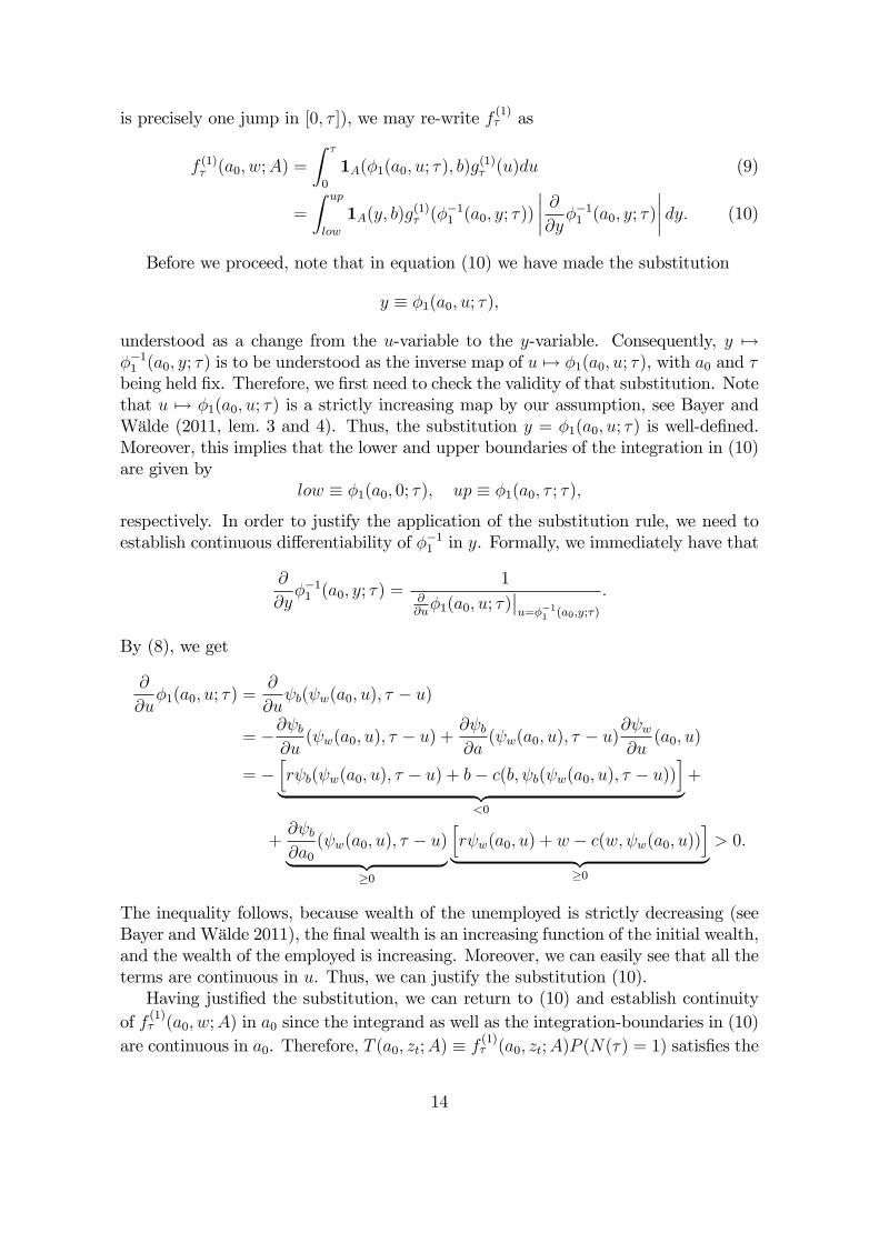
is precisely one jump in [0; � ]), we may re-write f (1)� as

f (1)� (a0; w;A) =

Z �

0

1A(�1(a0; u; �); b)g(1)� (u)du (9)

=

Z up

low

1A(y; b)g(1)� (�

�11 (a0; y; �))

���� @@y��11 (a0; y; �)���� dy: (10)

Before we proceed, note that in equation (10) we have made the substitution

y � �1(a0; u; �);

understood as a change from the u-variable to the y-variable. Consequently, y 7!��11 (a0; y; �) is to be understood as the inverse map of u 7! �1(a0; u; �), with a0 and �being held �x. Therefore, we �rst need to check the validity of that substitution. Notethat u 7! �1(a0; u; �) is a strictly increasing map by our assumption, see Bayer andWälde (2011, lem. 3 and 4). Thus, the substitution y = �1(a0; u; �) is well-de�ned.Moreover, this implies that the lower and upper boundaries of the integration in (10)are given by

low � �1(a0; 0; �); up � �1(a0; � ; �);

respectively. In order to justify the application of the substitution rule, we need toestablish continuous di¤erentiability of ��11 in y. Formally, we immediately have that

@

@y��11 (a0; y; �) =

1@@u�1(a0; u; �)

��u=��11 (a0;y;�)

:

By (8), we get

@

@u�1(a0; u; �) =

@

@u b( w(a0; u); � � u)

= �@ b@u( w(a0; u); � � u) +

@ b@a( w(a0; u); � � u)

@ w@u

(a0; u)

= �hr b( w(a0; u); � � u) + b� c(b; b( w(a0; u); � � u))

i| {z }

<0

+

+@ b@a0

( w(a0; u); � � u)| {z }�0

hr w(a0; u) + w � c(w; w(a0; u))

i| {z }

�0

> 0:

The inequality follows, because wealth of the unemployed is strictly decreasing (seeBayer and Wälde 2011), the �nal wealth is an increasing function of the initial wealth,and the wealth of the employed is increasing. Moreover, we can easily see that all theterms are continuous in u. Thus, we can justify the substitution (10).Having justi�ed the substitution, we can return to (10) and establish continuity

of f (1)� (a0; w;A) in a0 since the integrand as well as the integration-boundaries in (10)are continuous in a0. Therefore, T (a0; zt;A) � f

(1)� (a0; zt;A)P (N(�) = 1) satis�es the

14

�rst condition in def. 3.8 �continuity in the z-variable is trivial. The second and thethird conditions are obvious, and we have �nished the proof of the lemma.We can now complete our proof of uniqueness by proving the remaining conditions

of prop. 3.9.

Theorem 4.5 Suppose that r < � and that c(a; z) is continuously di¤erentiable ina. Then there is a unique invariant probability measure for the wealth-employmentprocess (a(�); z(�)).

Proof. By lemma 4.2 and lemma 4.4, the employment-wealth process (a(�); z(�))is an irreducible T -process. Thus, prop. 3.9 implies that (a(�); z(�)) is Harris recur-rent, given that Px(Xt ! 1) = 0 holds for our bounded state space. By prop. 3.7,there is a unique invariant measure (up to a constant multiplier), and prop. 3.6, �-nally, implies that we may choose the invariant measure to be a probability measure.

4.3 Stability

Using the skeleton approach of prop. 3.13, we now show stability.

Corollary 4.6 Under the assumptions of theorem 4.5, the employment-wealth processis stable in the sense of def. 3.10.

Proof. Recall that the employment-wealth-process is a T -process, see lemma 4.4.Moreover, we have shown irreducibility in lemma 4.2. Proposition 3.13 will imply thedesired conclusion, if we can show irreducibility of a skeleton chain. Take any � > 0and consider the corresponding skeleton Yn, n 2 N, with transition probabilities P � .By the proof of lemma 4.4, we see that (Yn) is also a T -process, where the de�nitionof T -processes is generalized to discrete-time processes in the obvious way. By Meynand Tweedie (1993, prop. 6.2.1), the discrete-time T -process Y is irreducible if thereis a point x 2 X such that for any open neighborhood O of x, we have

8y 2 X : �1n=1Pn� (y;O) > 0: (11)

This property, however, can be easily shown for the wealth-employment process(a; z). Indeed, take x = (�b=r; b). Then any open neighborhood O of x contains[�b=r;�b=r + �[�fbg for some � > 0. We start at some point y = (a0; z0) 2 Xand assume the following scenario: if necessary, at some time between 0 and � , theemployment status changes to b, then it stays constant until the random time N�de�ned by N � inffn j a(n�) < �b=r + �g. Note that the wealth is decreasing ina deterministic way while z = b. Thus, we can �nd a deterministic upper boundN � K(a0). The event that the employment attains the value b during the timeinterval [0; � ] and retains this value until time K(a0)� has positive probability. Inthis case, however, the trajectory of the wealth-employment process reaches O, im-plying that �1n=1P

n� (y;O) > 0. Thus, the � -skeleton chain is irreducible and thewealth-employment process is stable.

15

5 Application to other models

Let us now apply the conditions obtained above for the existence, uniqueness andstability of an invariant distribution to other models used in the literature. The mod-els are chosen as they are either widely used or they have very useful properties. Westart with a geometric Brownian motion process which is extremely popular in theeconomics literature. It is not, however, characterized by an invariant unique and sta-ble distribution. It nevertheless does have, however, some other features which makesit very attractive. The subsequent section then presents a version of the Ornstein-Uhlenbeck process. This version also implies a lognormal distribution but it has allthe properties one would wish for. While there are some recent applications of theprocess, it is not as widely used as it should. The �nal example studies propertiesof a model driven by Poisson uncertainty. The structure of this model is somewhatsimpler than the one studied above. It is therefore especially useful for illustratingthe ideas of the above proofs. The concluding subsection points out why proofs ofstable invariant and unique distributions might fail for other modeling setups.

5.1 Geometric models

5.1.1 A geometric Brownian motion model

One of the most popular fundamental structures is the geometric Brownian motionmodel. Using capital K (t) as an example, its structure is

dK (t) = K (t) [gdt+ �dB (t)] ; (12)

where B (t) is standardized Brownian motion, i.e. B (t) � N (0; t) ; � is the constantvariance parameter and g is a constant which collects various parameters dependingon the speci�c model under consideration. This reduced form can be derived from orappears in the models in Evans and Kenc (2003), Gabaix (1999), Gertler and Grinols(1982), Gokan (2002), Gong and Zou (2002, 2003), Grinols and Turnovsky (1998a,1998b), Obstfeld (1994), Prat (2007), Steger (2005) or Turnovsky (1993) and manyothers. For more background and a critique, see Wälde (2011).It is well-known that the capital stock as described by (12) for any � > t given

a �xed initial condition of K (t) = K0 is log-normally distributed (this would alsohold for a random (log-normal) initial condition): As the solution to (12) is K (�) =

K0e(g� 1

2�2)(��t)+�z(�) (see e.g. Wälde, 2010, ch. 10.4.1) and B (t) is normally distrib-

uted, K (t) is lognormally distributed,

K (�) � logN��� ; �

2�

�� f (K; �) =

1

Kp2�2��

e� (logK��� )2

2�2� (13)

where the mean and variance of K (�) are (see app. A.1)

�� � � (�;K0) � EtK (�) = K0eg[��t]; (14)

�2� � �2 (�;K0) � vartK (�) = K20e2g[��t]

�e�

2[��t] � 1�: (15)

16

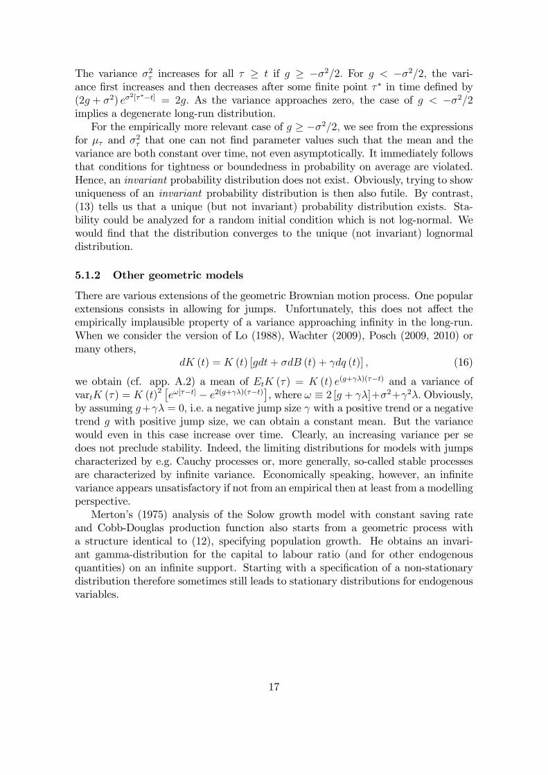
The variance �2� increases for all � � t if g � ��2=2: For g < ��2=2; the vari-ance �rst increases and then decreases after some �nite point � � in time de�ned by(2g + �2) e�

2[���t] = 2g: As the variance approaches zero, the case of g < ��2=2implies a degenerate long-run distribution.For the empirically more relevant case of g � ��2=2; we see from the expressions

for �� and �2� that one can not �nd parameter values such that the mean and thevariance are both constant over time, not even asymptotically. It immediately followsthat conditions for tightness or boundedness in probability on average are violated.Hence, an invariant probability distribution does not exist. Obviously, trying to showuniqueness of an invariant probability distribution is then also futile. By contrast,(13) tells us that a unique (but not invariant) probability distribution exists. Sta-bility could be analyzed for a random initial condition which is not log-normal. Wewould �nd that the distribution converges to the unique (not invariant) lognormaldistribution.

5.1.2 Other geometric models

There are various extensions of the geometric Brownian motion process. One popularextensions consists in allowing for jumps. Unfortunately, this does not a¤ect theempirically implausible property of a variance approaching in�nity in the long-run.When we consider the version of Lo (1988), Wachter (2009), Posch (2009, 2010) ormany others,

dK (t) = K (t) [gdt+ �dB (t) + dq (t)] ; (16)

we obtain (cf. app. A.2) a mean of EtK (�) = K (t) e(g+ �)(��t) and a variance ofvartK (�) = K (t)2

�e![��t] � e2(g+ �)(��t)

�, where ! � 2 [g + �]+�2+ 2�: Obviously,

by assuming g+ � = 0; i.e. a negative jump size with a positive trend or a negativetrend g with positive jump size, we can obtain a constant mean. But the variancewould even in this case increase over time. Clearly, an increasing variance per sedoes not preclude stability. Indeed, the limiting distributions for models with jumpscharacterized by e.g. Cauchy processes or, more generally, so-called stable processesare characterized by in�nite variance. Economically speaking, however, an in�nitevariance appears unsatisfactory if not from an empirical then at least from a modellingperspective.Merton�s (1975) analysis of the Solow growth model with constant saving rate

and Cobb-Douglas production function also starts from a geometric process witha structure identical to (12), specifying population growth. He obtains an invari-ant gamma-distribution for the capital to labour ratio (and for other endogenousquantities) on an in�nite support. Starting with a speci�cation of a non-stationarydistribution therefore sometimes still leads to stationary distributions for endogenousvariables.

17

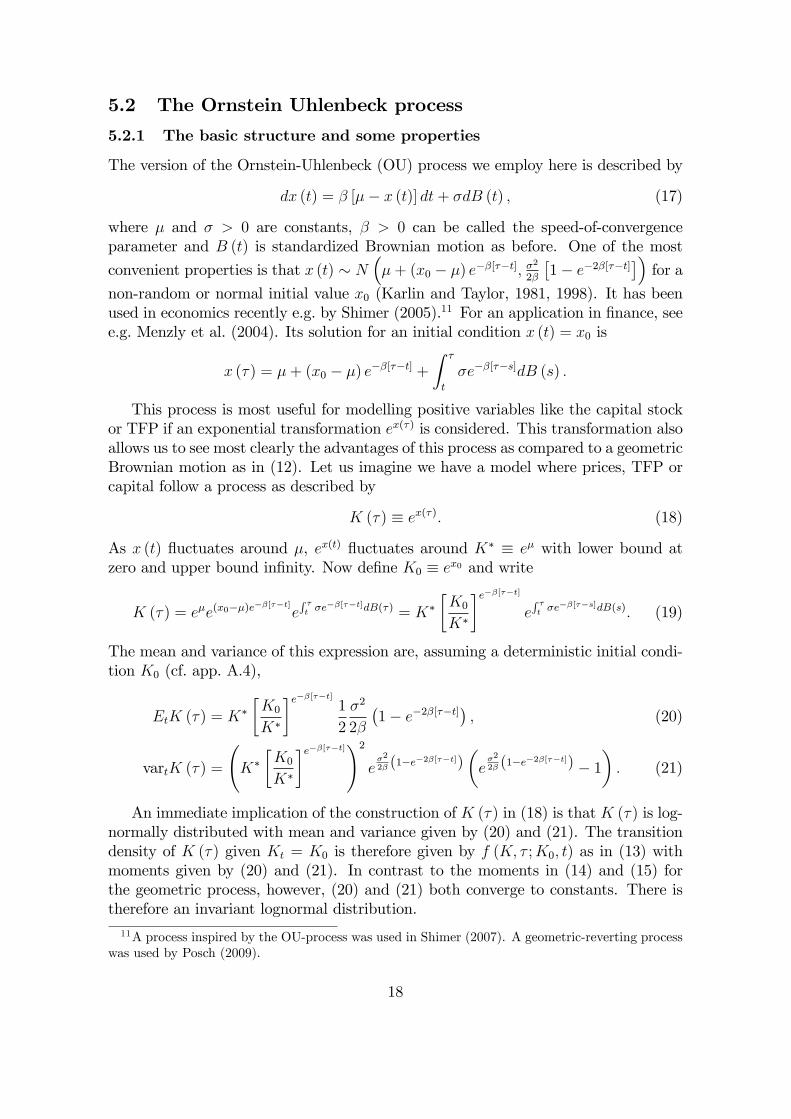
5.2 The Ornstein Uhlenbeck process

5.2.1 The basic structure and some properties

The version of the Ornstein-Uhlenbeck (OU) process we employ here is described by

dx (t) = � [�� x (t)] dt+ �dB (t) ; (17)

where � and � > 0 are constants, � > 0 can be called the speed-of-convergenceparameter and B (t) is standardized Brownian motion as before. One of the most

convenient properties is that x (t) � N��+ (x0 � �) e��[��t]; �

2

2�

�1� e�2�[��t]

��for a

non-random or normal initial value x0 (Karlin and Taylor, 1981, 1998). It has beenused in economics recently e.g. by Shimer (2005).11 For an application in �nance, seee.g. Menzly et al. (2004). Its solution for an initial condition x (t) = x0 is

x (�) = �+ (x0 � �) e��[��t] +

Z �

t

�e��[��s]dB (s) :

This process is most useful for modelling positive variables like the capital stockor TFP if an exponential transformation ex(�) is considered. This transformation alsoallows us to see most clearly the advantages of this process as compared to a geometricBrownian motion as in (12). Let us imagine we have a model where prices, TFP orcapital follow a process as described by

K (�) � ex(�): (18)

As x (t) �uctuates around �, ex(t) �uctuates around K� � e� with lower bound atzero and upper bound in�nity. Now de�ne K0 � ex0 and write

K (�) = e�e(x0��)e��[��t]

eR �t �e

��[��t]dB(�) = K��K0

K�

�e��[��t]eR �t �e

��[��s]dB(s): (19)

The mean and variance of this expression are, assuming a deterministic initial condi-tion K0 (cf. app. A.4),

EtK (�) = K��K0

K�

�e��[��t]1

2

�2

2�

�1� e�2�[��t]

�; (20)

vartK (�) =

K��K0

K�

�e��[��t]!2e�2

2� (1�e�2�[��t])�e�2

2� (1�e�2�[��t]) � 1�: (21)

An immediate implication of the construction of K (�) in (18) is that K (�) is log-normally distributed with mean and variance given by (20) and (21). The transitiondensity of K (�) given Kt = K0 is therefore given by f (K; � ;K0; t) as in (13) withmoments given by (20) and (21). In contrast to the moments in (14) and (15) forthe geometric process, however, (20) and (21) both converge to constants. There istherefore an invariant lognormal distribution.11A process inspired by the OU-process was used in Shimer (2007). A geometric-reverting process

was used by Posch (2009).

18

5.2.2 Conditions for existence, uniqueness and stability

After these preliminary steps, we will now illustrate the proofs of section 3.2 andapply them to the exponential OU process. While sections 3.2 and 4 have alreadyshown the line of thought, we brie�y recapitulate what needs to be proven. Thefollowing can also be seen as a �check-list�of conditions to be checked by authors ofother models.Consider a Markov process X:We need to investigate whether it has the following

properties.1) X is bounded in probability on average2) X has the weak Feller property3) X is a '-irreducible T -process4) There is a skeleton chain of process X which is irreducible.

Property 1 and 2 (by prop. 3.6) imply the existence of an invariant probability measure.Properties 3 and the growth condition Px(Xt ! 1) = 0 for every x 2 R imply theexistence of a unique invariant measure (by prop. 3.7 via prop. 3.9). As this growthcondition is implied by the stronger property 1, we will establish the existence of aunique invariant measure by checking properties 1 and 3. Properties 1 to 3 imply theexistence of a unique invariant probability measure. Property 4 implies stability of aninvariant distribution by prop. 3.13.Existence - The Markov process K of this application is described by (18) with

(17). It is tight as discussed after def. 3.4: Fix an initial condition K0 and an � > 0:A set C for which PK0(K (�1) 2 C) = 1� � for some �1 can trivially be found. If thevariance and mean, and thereby the entire distribution, stay constant, the same setis characterized by PK0(K (t) 2 C) � 1� � for all t. As X is tight, it is also �boundedin probability on average�.The process K also has the weak Feller property: K (t) is an Ito di¤usion (Øk-

sendal, 1998, 5th edition, ch. 7.1) and �any Ito di¤usion is Feller-continuous� (Øk-sendal, 1998, 5th edition, lem. 8.1.4). As Feller-continuous is a di¤erent name for weakFeller property, we conclude that a long-run invariant probability measure exists.Uniqueness - We now argue that K is a '-irreducible T -process. We can follow

the arguments in the proof of lemma 4.2 to �rst show '-irreducibility: For any initialcondition K0; there is a positive probability to reach any subset of the state space in�nite time, essentially by irreducibility of the underlying Brownian motion. Using asmeasure � the Lebesgue measure, for instance, we have established irreducibility ofK:12

To show that K is a T -process, def. 3.8 tells us that we need to �nd a functionT (K;A) which satis�es the three conditions of this de�nition. The function shouldbe positive, continuous and smaller than K� (K0; A) �

R10P � (K0; A) � (d�) for any

initial condition K0, any set A and a suitable probability measure �: The latter

12In contrast to our original setup of section 2, the OU-process x here is uniformly elliptic. Thisimmediately implies irreducibility for x and also K. Indeed, by the results of Kusuoka and Stroock(1987), we see that the transition density of x is bounded below (and above) by a Gaussian transitiondensity. Thus, it is positive, implying irreducibility. Of course, in the case of an OU-process, we candirectly write down the transition density and verify its positivity.

19

measure is completely unrelated to the probability measure implicit in P � (K0; A) :Let us �rst compute P � (K0; A) for (18). Using the lognormal density of (13), we

get

P � (K0; A) =

ZA

f (K; �) dK: (22)

Integrating yieldsR10P � (K0; A) � (d�) =

R10

RAf (K; �) dK�(d�): Now imagine that

v is a smooth probability measure with support [0;1[. We can then write thisexpression as

R10

RAf (K; �) dK� (�) d�: As the density f (K; �) de�ned in (13), using

the mean and variance from (20) and (21), is continuous in K0 and integrating in (22)preserves this continuity and so does integration with a smooth probability measurev (�) ; the function K� (K0; A) itself is continuous in K0: Taking it as our function

T�K̂; A

�; we found again a T -process. This establishes the existence of a unique

invariant probability measure.It is worth noting at this point that the application of T -processes for processes

driven only by Brownian motion (i.e. there are no jumps) is somewhat �unusual�.Our process K actually has the strong Feller property, which is much stronger thanthe T -property. Indeed, this is a common feature of all so-called hypo-elliptic dif-fusion processes, see, for instance, Meyn and Tweedie (1993b). Hypo-ellipticity is ageneralization of ellipticity, which is satis�ed here.Stability - The skeleton chain is constructed by �xing a � > 0 and considering

the process Yn � K (�n) with n 2 N. As we have noted above, the transitiondensities of K are strictly positive. Thus, the transition density of Y is positive,which immediately implies irreducibility.Consider the following example. We start in y = K0 and consider a neighborhood

O =��K; �K + "

�with some " > 0: Then P n�

�K0;

��K; �K + "

��=R �K+"�K

f (K;n�) :Given the density de�ned in (13) with (20) and (21), this probability is strictly posi-tive. As this works for any �K > 0; we have shown stability.

5.3 A model of natural volatility

The following model is characterized by jumps as well. The strong Feller propertytherefore does not hold and the application of the tools of section 3 and 4 is needed.

5.3.1 Basic structure and some properties

The natural volatility literature stresses that growth and volatility are two sides ofthe same coin. Determinants of long-run growth are also determinants of short-runvolatility. Both short-run volatility and long-run growth are endogenous. This pointhas been made in the papers of Bental and Peled (1996), Matsuyama (1999), Wälde(2002, 2005), Francois and Lloyd-Ellis (2003,2008), Posch and Wälde (2009) andothers. The (slightly simpli�ed) reduced form of the models by Wälde (2005) andPosch and Wälde (2009) reads

dK̂ (�) =�K̂ (�)� � �1K̂ (�)

�dt� �2K̂ (�) dq; (23)

20

where K̂ is the (stochastically detrended) capital stock, q is a Poisson process withsome constant (but endogenous) arrival rate and 0 < �; �i < 1 are constant parame-ters.This equation immediately reveals that in times without jumps (dq = 0) and an

initial capital stock of K̂0 < K̂� � ��1=(1��)1 ; the capital stock monotonically increases

over time to asymptotically approach K̂�: When there is a jump, the (stochasticallydetrended) capital stock reduces by �2 percent. We also see that the range of the

capital stock with an initial condition given by 0 < K̂0 < K̂� is given byi0; K̂�

h:

5.3.2 Conditions for existence, uniqueness and stability

The Markov process K̂ of this application is described by (23). We follow our �check-list�of ch. 5.2.2.Existence - The process K̂ is bounded in probability on average as its state spacei

0; K̂�his �nite. The process K̂ also has the weak Feller property as it has the same

properties as shown in 4.1: With �xed !; i.e. �xed jump-times, K̂ (�) is a continuousfunction of the initial condition K̂0. Second, for any bounded and continuous functionf :i0; K̂�

h! R; the mean E

�f�K̂ (�)

��is a continuous function in K̂0: The proof

follows exactly, mutatis mutandis, the same steps as the arguments in the proof oflemma 4.1. This implies existence of an invariant probability measure.Uniqueness - Let us establish that K̂ is a '-irreducible T -process. We can follow

the arguments in the proof of lemma 4.2 to �rst show '-irreducibility: Let the statespace be R�0. Regardless of the initial point K (t) 2 R�0, it is possible to attain thestate K (�) in �nite time with probability greater than zero. Thus, prop. 3.2 impliesirreducibility, where we can take the Lebesgue measure on R�0 as measure �.To show that K̂ is a T -process, def. 3.8 tells us that we need to �nd a function

T�K̂; A

�which satis�es the three conditions of this de�nition. Using the same Dirac

measure as before in the proof of lem. 4.4, v = �� , the three conditions requirethat T

�K̂; A

�be continuous with Ka

�K̂;A

��R10P t(x;A)�� (dt) = P �

�K̂; A

��

T�K̂; A

�> 0.

The idea for �nding such a function is also borrowed from lem. 4.4: We considerthe probability that K̂ (�) 2 A for some � > t. We decompose it as in (6) into

P�K̂ (�) 2 AjK̂(t) = K̂0

�= �1k=0P

�K̂ (�) 2 AjK̂(t) = K̂0; N (�) = k

�P (N(�) = k)

and argue that T�K̂;A

�� P

�K̂ (�) 2 AjK̂(t) = K̂0; N (�) = 1

�P (N(�) = 1) is

continuous in K̂0: Given that T�K̂;A

�is the product of two probabilities, it is

positive. As T�K̂;A

�� P

�K̂ (�) 2 AjK̂(t) = K̂0

�= Ka

�K̂;A

�; we are done and

21

have established that K̂ is a T -process. All of this implies that K̂ has a unique in-variant measure. Combined with the existence of an invariant probability measure,we can conclude that there is a unique invariant probability measure.Stability - This works as in the OU-case above. We construct a skeleton chain and

see that it is a T -process. Then we argue that we can reach any neighborhood witha positive probability. This establishes stability.

6 Conclusion

This paper has introduced methods that allow to prove existence, uniqueness andstability of distributions described by stochastic di¤erential equations which resultfrom the solution of an optimal control problem. These methods are �rst appliedto a matching and saving model. Existence, uniqueness and stability of the optimalprocess for the state variables, wealth and labour market status, were proven. Weproceed by applying these methods to three model classes from the literature. Weshow that proving existence, uniqueness and stability is relatively straightforward,following the steps in the detailed proofs for the matching model.We �nally provide some caveats about sensible issues for more complex models

than the ones used here. Properties 3 and 4 of our �check list� imply Harris re-currence which is crucial for uniqueness. It is well-known that Brownian motion ofdimension three or higher is not recurrent, see Øksendal (1998, Example 7.4.2). Asa consequence, one can easily �nd two functions (and any linear combination withpositive coe¢ cients) that are densities of invariant measures of the three-dimensionalBrownian motion.The T -property is especially useful for models where randomness is introduced

by �nite-activity jump processes, i.e., by compound Poisson processes. In di¤usionmodels, usually even the strong Feller property holds, which makes it easy to con-clude the T -property. On the other hand, in models driven by in�nite-activity jumpprocesses, e.g., Lévy processes with in�nite activity, it does not seem clear whetherthe T -property can lead to useful results. Indeed, in these models, the strong Fellerproperty may and may not hold, see, for instance, Picard (1995/97). On the otherhand, the weak Feller property is satis�ed for all Lévy processes, implying existenceof invariant distributions, see Applebaum (2004, theorem 3.1.9). Looking at theseissues in economic applications o¤ers many fascinating research projects for years tocome.

A Appendix

- see after references -

22

References

Alvarez, F., and R. Shimer (2011): �Search and Rest Unemployment,�Econometrica,79, 75�122.

Applebaum, D. (2004): Lévy processes and stochastic calculus, vol. 93 of CambridgeStudies in Advanced Mathematics. Cambridge University Press, Cambridge.

Azema, J., M. Du�o, and D. Revuz (1969): �Mesure invariante des processus deMarkov recurrents.,� Sem. Probab. III, Univ. Strasbourg 1967/68, Lect. NotesMath. 88, 24-33 (1969).

Bandi, F. M., and T. H. Nguyen (2003): �On the functional estimation of jump-di¤usion models,�Journal of Econometrics, 116(1-2), 293�328.

Bayer, C., and K. Wälde (2011): �Describing the Dynamics of Distributions inSearch and Matching Models by Fokker-Planck Equations,�mimeo - available atwww.waelde.com/pub.

Bental, B., and D. Peled (1996): �The Accumulation of Wealth and the CyclicalGeneration of New Technologies: A Search Theoretic Approach,� InternationalEconomic Review, 37, 687�718.

Bhattacharya, R., andM.Majumdar (2004): �Random dynamical systems: a review,�Economic Theory, 23(1), 13�38.

Bismut, J.-M. (1975): �Growth and Optimal Intertemporal Allocation of Risks,�Journal of Economic Theory, 10(2), 239�257.

Brock, W., and M. Magill (1979): �Dynamics under Uncertainty,� Econometrica,47(4), 843�868.

Brock, W., and L. Mirman (1972): �Optimal Economic Growth and Uncertainty: TheDiscounted Case,�Journal of Economic Theory, 4(3), 479�513.

Burdett, K., C. Carrillo-Tudela, and M. G. Coles (forthcoming): �Human CapitalAccumulation and Labour Market Equilibrium,�International Economic Review.

Burdett, K., and D. T. Mortensen (1998): �Wage Di¤erentials, Employer Size, andUnemployment,�International Economic Review, 39, 257�273.

Cahuc, P., F. Postel-Vinay, and J.-M. Robin (2006): �Wage Bargaining with On-the-job Search: Theory and Evidence,�Econometrica, 74, 323�365.

Chang, F.-R., and A. Malliaris (1987): �Asymptotic Growth under Uncertainty: Ex-istence and Uniqueness,�Review of Economic Studies, 54(1), 169�174.

Coles, M. G., and D. T. Mortensen (2011): �Dynamic Monopsonistic Competitionand Labor Market Equilibrium,�mimeo.

23

Down, D., S. P. Meyn, and R. L. Tweedie (1995a): �Exponential and Uniform Er-godicity of Markov Processes,�Annals of Probability, 23, 1671 �1691.

(1995b): �Exponential and uniform ergodicity of Markov processes,�Ann.Probab., 23(4), 1671�1691.

Evans, L., and T. Kenc (2003): �Welfare cost of monetary and �scal policy shocks,�Macroeconomic Dynamics, 7(2), 212�238.

Francois, P., and H. Lloyd-Ellis (2003): �Animal Spirits Trough Creative Destruc-tion,�American Economic Review, 93, 530�550.

(2008): �Implementation Cycles, Investment, And Growth,� InternationalEconomic Review, 49(3), 901�942.

Futia, C. (1982): �Invariant Distributions and the Limiting Behavior of MarkovianEconomic Models,�Econometrica, 50(2), 377�408.

Gabaix, X. (1999): �Zipf�s Law For Cities: An Explanation,�Quarterly Journal ofEconomics, 114(3), 739�767.

García, M. A., and R. J. Griego (1994): �An Elementary Theory of Stochastic Dif-ferential Equations Driven by A Poisson Process,�Communications in Statistics -Stochastic Models, 10(2), 335�363.

Gertler, M., and E. Grinols (1982): �Monetary randomness and investment,�Journalof Monetary Economics, 10(2), 239�258.

Gokan, Y. (2002): �Alternative government �nancing and stochastic endogenousgrowth,�Journal of Economic Dynamics and Control, 26(4), 681�706.

Gong, L., and H.-F. Zou (2002): �Direct preferences for wealth, the risk premium puz-zle, growth, and policy e¤ectiveness,�Journal of Economic Dynamics and Control,26(2), 247�270.

(2003): �Military spending and stochastic growth,� Journal of EconomicDynamics and Control, 28(1), 153�170.

Grinols, E. L., and S. J. Turnovsky (1998): �Consequences of debt policy in a sto-chastically growing monetary economy,� International Economic Review, 39(2),495�521.

(1998b): �Risk, Optimal Government Finance and Monetary Policies in aGrowing Economy,�Economica, 65(259), 401�427.

Hansen, L. P., and J. A. Scheinkman (2009): �Long-Term Risk: An Operator Ap-proach,�Econometrica, 77(1), 177�234.

Hopenhayn, H., and E. Prescott (1992): �Stochastic Monotonicity and StationaryDistributions for Dynamic Economies,�Econometrica, 60(6), 1387�1406.

24

Huggett, M. (1993): �The risk-free rate in heterogeneous-agent incomplete-insuranceeconomies,�Journal of Economic Dynamics and Control, 17, 953�969.

Kaas, L., and P. Kircher (2011): �E¢ cient Firm Dynamics in a Frictional LaborMarket,�mimeo Konstanz and LSE.

Karlin, S., and H. Taylor (1981): A second course in stochastic modeling. AcademicPress.

(1998): An introduction to stochastic modeling. Academic Press, 3rd ed.

Kusuoka, S., and D. Stroock (1987): �Applications of the Malliavin calculus. III,�J.Fac. Sci. Univ. Tokyo Sect. IA Math., 34(2), 391�442.

Lentz, R. (2010): �Sorting by search intensity,�Journal of Economic Theory, 145(4),1436�1452.

Lo, A. W. (1988): �Maximum likelihood estimation of generalized Ito processes withdiscretely sampled data,�Econometric Theory, 4, 231�247.

Magill, M. (1977): �A Local Analysis of N-Sector Capital Accumulation under Un-certainty,�Journal of Economic Theory, 15(1), 211�219.

Matsuyama, K. (1999): �Growing Through Cycles,�Econometrica, 67, 335�347.

Menzly, L., T. Santos, and P. Veronesi (2004): �Understanding Predictability,�Jour-nal of Political Economy, 112(1), 1�47.

Merton, R. C. (1975): �An Asymptotic Theory of Growth under Uncertainty,�TheReview of Economic Studies, 42(3), 375�393.

Meyn, S. P., and R. L. Tweedie (1993a): Markov chains and stochastic stability,Communications and Control Engineering Series. Springer-Verlag London Ltd.,London.

Meyn, S. P., and R. L. Tweedie (1993b): �Stability of Markovian processes. II.Continuous-time processes and sampled chains,� Adv. in Appl. Probab., 25(3),487�517.

(1993c): �Stability of Markovian processes. III. Foster-Lyapunov criteria forcontinuous-time processes,�Adv. in Appl. Probab., 25(3), 518�548.

Moscarini, G. (2005): �Job Matching and the Wage Distribution,� Econometrica,73(2), 481�516.

Moscarini, G., and F. Postel-Vinay (2008): �The Timing of Labor Market Expansions:New Facts and a New Hypothesis,�NBER Macroeconomic Annual 23.

(2010): �Stochastic Search Equilibrium,�mimeo Bristol and Yale.

25

Nishimura, K., and J. Stachurski (2005): �Stability of stochastic optimal growthmodels: a new approach,�Journal of Economic Theory, 122(1), 100�118.

Obstfeld, M. (1994): �Risk-Taking, Global Diversi�cation, and Growth,�AmericanEconomic Review, 84, 1310�29.

Øksendal, B. (1998): Stochastic Di¤erential Equations. Springer, Fifth Edition,Berlin.

Olson, L., and S. Roy (2006): �Theory of Stochastic Optimal Economic Growth,�inHandbook of Optimal Growth, Vol. I: Discrete Time, ed. by R. A. Dana, C. L.Van, T. Mitra, and K. Nishimura. Springer, Berlin.

Picard, J. (1995/97): �Density in small time for Levy processes,� ESAIM Probab.Statist., 1, 357�389 (electronic).

Pissarides, C. A. (1985): �Short-run Equilibrium Dynamics of Unemployment Vacan-cies, and Real Wages,�American Economic Review, 75, 676�90.

Posch, O. (2009): �Structural estimation of jump-di¤usion processes in macroeco-nomics,�Journal of Econometrics, 153, 196�210.

Posch, O., and K. Wälde (2009): �On the Non-Causal Link between Volatility andGrowth,� University of Aarhus and University of Louvain la Neuve, DiscussionPaper.

Postel-Vinay, F., and J.-M. Robin (2002): �EquilibriumWage Dispersion with Workerand Employer Heterogeneity,�Econometrica, 70, 2295�2350.

Prat, J. (2007): �The impact of disembodied technological progress on unemploy-ment,�Review of Economic Dynamics, 10, 106�125.

Rishel, R. (1970): �Necessary and Su¢ cient Dynamic Programming Conditions forContinuous Time Stochastic Optimal Control,�SIAM Journal on Control and Op-timization, 8(4), 559�571.

Scott, L. O. (1987): �Option Pricing when the Variance Changes Randomly: Theory,Estimation, and an Application,�Journal of Financial and Quantitative Analysis,22(4), 419�438.

Shimer, R. (2005): �The Cyclical Behavior of Equilibrium Unemployment and Va-cancies,�American Economic Review, 95, 25�49.

(2007): �Mismatch,�American Economic Review, 97(4), 1074�1101.

Shimer, R., and L. Smith (2000): �Assortative Matching and Search,�Econometrica,68(2), 343�369.

Steger, T. M. (2005): �Stochastic growth under Wiener and Poisson uncertainty,�Economics Letters, 86(3), 311�316.

26

Turnovsky, S. J. (1993): �Macroeconomic policies, growth, and welfare in a stochasticeconomy,�International Economic Review, 34(4), 953�981.

Wachter, J. A. (2009): �Can time-varying risk of rare disasters explain aggregatestock market volatility?,�mimeo Wharton School.

Wälde, K. (2002): �The economic determinants of technology shocks in a real businesscycle model,�Journal of Economic Dynamics and Control, 27(1), 1�28.

(2005): �Endogenous Growth Cycles,� International Economic Review, 46,867�894.

(2010): Applied Intertemporal Optimization. Gutenberg University Press,available at www.waelde.com/aio.

(2011): �Production technologies in stochastic continuous time models,�Journal of Economic Dynamics and Control, 35, 616�622.

27

A Appendix

forExistence, uniqueness and stability of invariant distributions

in continuous-time stochastic models

by

Christian Bayer(a) and Klaus Wälde(b)

July 21, 2011

This appendix contains various derivations omitted in the main part.

A.1 Mean and variance in (14) and (15)

Consider the geometric Brownian process (12). Given the solutionK (�) = K0e(g� 1

2�2)(��t)+�z(�),

we would now like to know what the expected level K (�) in � from the perspectiveof t is. To this end, apply the expectations operator Et and �nd

EtK (�) = K0E0e(g� 1

2�2)(��t)+�z(�) = K0e

(g� 12�2)(��t)E0e

�z(�); (24)

where the second equality exploited the fact that e(g�12�2)(��t) is non-random. As z (�)

is standard normally distributed, z (�) ~N (0; � � t), �z (�) is normally distributedwith N (0; �2 [� � t]) : As a consequence, e�z(�) is log-normally distributed with meane12�2[��t] (see e.g. Wälde, 2010, ch. 7.3.3). Hence,

EtK (�) = K0e(g� 1

2�2)(��t)e

12�2[��t] = K0e

g[��t]: (25)

Note that we can also determine the variance of K (�) by simply applying thevariance operator to the solution for K (�),

vartK (�) = vart�K0e

(g� 12�2)(��t)e�z(�)

�= K2

0e2(g� 1

2�2)(��t)vart

�e�z(�)

�:

We nowmake similar arguments to before when we derived (25). As �B (t) ~N (0; �2 [� � t]) ;

the term e�z(�) is log-normally distributed with variance e�2[��t]

�e�

2[��t] � 1�: Hence,

we �nd

vartK (�) = K20e2(g� 1

2�2)[��t]e�

2[��t]�e�

2[��t] � 1�= K2

0e(2(g� 1

2�2)+�2)[��t]

�e�

2[��t] � 1�

= K20e2g[��t]

�e�

2[��t] � 1�:

We see that even with g = 0 where K (�) is a martingale, i.e. for EtK (�) = K0;the variance increases over time. The variance also obviously increases for g > 0: Tounderstand the case of a negative g; we write the variance as

�2� = K20

he(2g+�

2)[��t] � e2g[��t]i:

28

This shows that as long as 2g+�2 � 0, (0 >) g � ��2=2; the variance also increasesas the �rst term, e(2g+�

2)[��t]; increases and the second term, e2g[��t]; falls and theminus sign implies that �2� unambiguously rises. For g < ��2=2; we have ambiguouse¤ects. Computing the time � derivative gives

d

d�vartK (�) = K2

0

��2g + �2

�e(2g+�

2)[��t] � 2ge2g[��t]�� 0,�

2g + �2�e�

2[��t] � 2g:

This inequality is satis�ed for � �close to�t but is violated for � su¢ ciently large. Inother words, the variance �rst increases and then falls.As a remark - life would be easier when we consider the log solution. It reads

lnK (t) = lnK0 +

�g � 1

2�2�t+ �B (t) :

The mean and variance of the log is simply

Et lnK (�) =

�g � 1

2�2�(� � t) ;

var (lnK (�)) = �2 [� � t] :

Here, the variance unambiguously increases.

A.2 The mean and variance of (16)

� The mean

Consider (16), reproduce here, dK (t) = K (t) [gdt+ �dB (t) + dq (t)] : The inte-gral version reads

K (�)�K (t) =

Z �

t

K (s) gds+

Z �

t

K (s)�dB (s) +

Z �

t

K (s) dq (s) :

Forming expectations yields with � (u) � EtK (u) and EtR �tK (s)�dB (s) = 0 from

the martingale property ofR �tK (s)�dB (s) andEt

R �tK (s) dq (s) =

R �tEtK (s) �ds

from the martingale properties of Poisson processes (e.g. Garcia and Griego, 1994 orWälde, 2010, ch. 10.5.3) with � being the arrival rate of the Poisson process

� (�)� � (t) =

Z �

t

� (s) gds+

Z �

t

� (s) �ds:

Di¤erentiating with respect to time � gives _� (�) = � (�) g + � (�) � and solvingyields

EtK (�) = K (t) e(g+ �)(��t): (26)

29

� The variance

Computing the variance is based on

vartK (�) = Et�K (�)2

�� (EtK (�))2 = Et

�K (�)2

��K (t)2 e2(g+ �)(��t): (27)

The process for K (t)2 with F (K (t)) = K (t)2 and (16) is given by (this is an appli-cation of a change-of-variable formula (CVF) for a combined jump-di¤usion process.See e.g. Wälde, 2010, ch. 10.2.4)

dK (t)2 = dF (K (t))

=

�F 0 (K (t)) gK (t) +

1

2F 00 (K (t))�2K (t)2

�dt

+ F 0 (K (t))�K (t) dB (t) + [F ((1 + )K (t))� F (K (t))] dq (t)

=�2gK (t)2 + �2K (t)2

dt+ 2�K (t)2 dB (t) +

�(1 + )2K (t)2 �K (t)2

�dq (t),

d� (t) =�2g + �2

�� (t) dt+ 2�� (t) dB (t) + (2 + ) � (t) dq (t)

where we de�ned � (t) � K (t)2 for simplicity. The integral version reads

� (�)� � (t) =�2g + �2

� Z �

t

� (s) ds+ 2�

Z �

t

� (s) dB (s) + (2 + )

Z �

t

� (s) dq (s) :

With expectations, we get

Et� (�)� � (t) =�2g + �2

� Z �

t

Et� (s) ds+ (2 + )

Z �

t

Et� (s)�ds:

The time � derivative gives

d

d�Et� (�) =

�2g + �2

�Et� (�) + (2 + ) �Et� (�) :

Solving this yields with ! � 2g + �2 + (2 + ) � = 2 [g + �] + �2 + 2�

Et� (�) = Et� (t) e![��t] , EtK (�)

2 = K (t)2 e![��t]:

The expectations operator in front of K (t)2 was dropped as the latter is known in t:Returning to (27), the variance therefore reads

vartK (�) = K (t)2�e![��t] � e2(g+ �)(��t)

�: (28)

Can we be sure that vartK (�) � 0? (We know that this must hold by de�nition, butour calculations might contain an error.) Let�s see,

vartK (�) � 0, e![��t] � e2(g+ �)(��t) , ! = 2g + �2 + (2 + ) � � 2 (g + �)

, �2 + 2 �+ 2� � 2 �, �2 + 2� � 0

which holds as the arrival rate � is positive.

30

� Is there an invariant distribution?

There are two necessary conditions for the distribution to be invariant in thelimit. The mean (26) is constant over time if g + � = 0 which is possible fornegative jump size or for a negative trend g with positive jumps. The variance (28)is constant, assuming a constant mean with g + � = 0 and the implication that! = 2g + �2 � (2 + ) g = �2 � g, if

vartK (�) = K (t)2he(�

2� g)[��t] � 1i:

Note that g + � = 0 implies that (remember that � � 0) either g or are negative(i.e. either there is a negative trend and positive jumps or a positive trend and negativejumps). This implies that g is negative and therefore �2 � g > 0: In other words,adding jumps allows to obtain a constant mean but does not allow to make thevariance converge to a constant. Adding jumps to a geometric Brownian motiontherefore does not imply an invariant distribution.

A.3 The di¤erential of (18)

To compare the process K (�) to the geometric Brownian motion in (12), we computeits di¤erential. We need to bring (18) into a form which allows us to apply theappropriate version of Ito�s Lemma (see Wälde, 2010, eq. 10.2.3). Use the expressiondx (t) = � [�� x (t)] dt+ �dB (t) from (17) and K (t) � F (x (t)) = ex(t): Ito�s lemmathen gives

dK (t) = dF (x (t)) =

�Fx (x (t)) � [�� x (t)] +

1

2Fxx (x (t))�

2

�dt+Fx (x (t))�dB (t) :

Inserting the �rst and second derivatives of F (x (t)) yields

dK (t) =

�ex(t)� [�� x (t)] +

1

2ex(t)�2

�dt+ ex(t)�dB (t),

dK (t) = K (t)

��� [�� lnK (t)] + 1

2�2�dt+ �dB (t)

�;

where the �i¤�reinserted K (t) = ex(t) and divided by K (t) :Obviously, the essential di¤erence to (12) consists in the term �� lnK (t)�. This

di¤erential representation also appears in the option pricing analysis of Scott (1987).

A.4 The mean and variance of (19)

Consider the solution of the exponentially transformed OU process in (19), i.e.

K (�) = K��K0

K�

�e��[��t]eR �t �e

��[��s]dB(s):

31

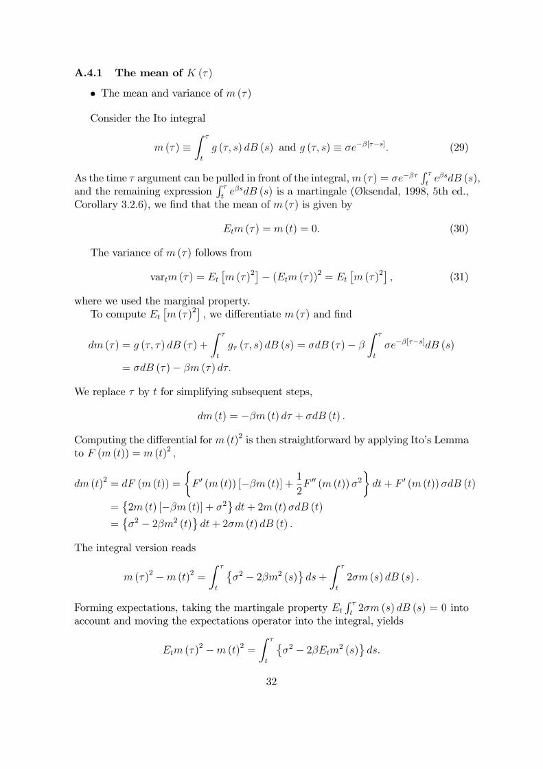
A.4.1 The mean of K (�)

� The mean and variance of m (�)

Consider the Ito integral

m (�) �Z �

t

g (�; s) dB (s) and g (�; s) � �e��[��s]: (29)

As the time � argument can be pulled in front of the integral,m (�) = �e���R �te�sdB (s),

and the remaining expressionR �te�sdB (s) is a martingale (Øksendal, 1998, 5th ed.,

Corollary 3.2.6), we �nd that the mean of m (�) is given by

Etm (�) = m (t) = 0: (30)

The variance of m (�) follows from

vartm (�) = Et�m (�)2

�� (Etm (�))2 = Et

�m (�)2

�; (31)

where we used the marginal property.To compute Et

�m (�)2

�; we di¤erentiate m (�) and �nd

dm (�) = g (�; �) dB (�) +

Z �

t

g� (�; s) dB (s) = �dB (�)� �

Z �

t

�e��[��s]dB (s)

= �dB (�)� �m (�) d�:

We replace � by t for simplifying subsequent steps,

dm (t) = ��m (t) d� + �dB (t) :

Computing the di¤erential form (t)2 is then straightforward by applying Ito�s Lemmato F (m (t)) = m (t)2 ;

dm (t)2 = dF (m (t)) =

�F 0 (m (t)) [��m (t)] + 1

2F 00 (m (t))�2

�dt+ F 0 (m (t))�dB (t)

=�2m (t) [��m (t)] + �2

dt+ 2m (t)�dB (t)

=��2 � 2�m2 (t)

dt+ 2�m (t) dB (t) :

The integral version reads

m (�)2 �m (t)2 =

Z �

t

��2 � 2�m2 (s)

ds+

Z �

t

2�m (s) dB (s) :

Forming expectations, taking the martingale property EtR �t2�m (s) dB (s) = 0 into

account and moving the expectations operator into the integral, yields

Etm (�)2 �m (t)2 =

Z �

t

��2 � 2�Etm2 (s)

ds:

32

Computing the time � derivative gives dd�Etm (�)

2 = �2 � 2�Etm2 (�) ; an ordinarydi¤erential equation in the second moment Etm (�)

2 : It can be solved to give

Etm (�)2 = Etm (t)

2 e�2�[��t] +

Z �

t

e�2�[��s]�2ds

=�2

2�

�1� e�2�[��t]

�:

The �nal equality used m (t)2 = 0 from (29).Returning to our original inquiry from (31) into determining the variance ofm (�),

we conclude

vartm (�) =�2

2�

�1� e�2�[��t]

�: (32)

The variance is zero for � = t and increases the larger � > t: It approaches �2=2� inthe limit.

� The mean of Etem(�)

Let us continue and compute Etem(�) with m (�) from (29). It is well-known thatthe Ito Integral m (�) is normally distributed. This means that em(�) is lognormallydistributed. We can then conclude that the mean of em(�) is given by

Etem(�) =

1

2

�2

2�

�1� e�2�[��t]

�(33)

� Finally, the mean of K (�)

Let us now compute the mean,

EtK (�) = K��K0

K�

�e��[��t]Ete

R �t �e

��[��s]dB(s): (34)

Given (33), we �nd

EtK (�) = K��K0

K�

�e��[��t]1

2

�2

2�

�1� e�2�[��t]

�:

A.4.2 The variance

Let us now compute the variance.

vartK (�) =

K��K0

K�

�e��[��t]!2vart

�em(�)

�:

As the Ito integral m (�) in (29) is normally distributed and mean and variance

are given by (30) and (32), we have m (�) � N�0; �

2

2�

�1� e�2�[��t]

��. Then, em(�) is

33

log-normally distributed with the mean being given by (33) and the variance of em(�)

is

vart�em(�)

�= e

�2

2� (1�e�2�[��t])�e�2

2� (1�e�2�[��t]) � 1�:

The variance of the capital stock is then

vartK (�) =

K��K0

K�

�e��[��t]!2e�2

2� (1�e�2�[��t])�e�2

2� (1�e�2�[��t]) � 1�:

34