-1-

57:020 Mechanics of Fluids & Transfer Processes

Exercise Notes for Fluid Property TM

Measurement of Density and Kinematic Viscosity Marian Muste, Surajeet Ghosh, Stuart Breczinski, and Fred Stern

1. Purpose

The purpose of this investigation is to provide Hands-on experience using a table-top facility and simple

measurement systems to obtain fluid property measurements (density and kinematic viscosity), comparing results

with manufacturer values, and implementing standard EFD uncertainty analysis. Additionally, this laboratory will

provide an introduction to camera settings and flow visualization for the ePIV system with a circular cylinder model.

2. Experimental Design

2.1 Part 1: For Determination of Fluid Properties

Common methods used for determining viscosity include the rotating-concentric-cylinder method (Engler

viscosimeter) and the capillary-flow method (Saybolt viscosimeter). In the present experiment we will measure the

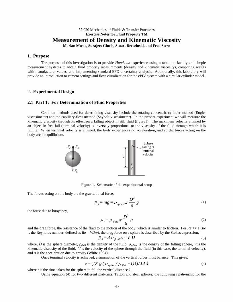
kinematic viscosity through its effect on a falling object in still fluid (figure1). The maximum velocity attained by

an object in free fall (terminal velocity) is inversely proportional to the viscosity of the fluid through which it is

falling. When terminal velocity is attained, the body experiences no acceleration, and so the forces acting on the

body are in equilibrium.

Figure 1. Schematic of the experimental setup

The forces acting on the body are the gravitational force,

g 6

D = mg = F sphereg

3

(1)

the force due to buoyancy,

g 6

D = F fluidb

3

(2)

and the drag force, the resistance of the fluid to the motion of the body, which is similar to friction. For Re << 1 (Re

is the Reynolds number, defined as Re = VD/ν), the drag force on a sphere is described by the Stokes expression,

D V 3 = F fluidd (3)

where, D is the sphere diameter, fluid is the density of the fluid, sphere is the density of the falling sphere, is the

kinematic viscosity of the fluid, V is the velocity of the sphere through the fluid (in this case, the terminal velocity),

and g is the acceleration due to gravity (White 1994).

Once terminal velocity is achieved, a summation of the vertical forces must balance. This gives:

18t 1) - /( g D = fluidsphere

2/)( (4)

where t is the time taken for the sphere to fall the vertical distance λ.

Using equation (4) for two different materials, Teflon and steel spheres, the following relationship for the

FF

F

V

Spherefalling atterminalvelocity

bd

g

-2-

density of the fluid is obtained, where subscripts s and t refer to the steel and Teflon spheres, respectively.

)/()(2

t D - tD t D - t D = s2sttss

2stt

2

tfluid (5)

In this experiment, we will drop spheres (Steel and Teflon), each set of spheres having a different density

and diameter, through a long transparent cylinder filled with glycerin (Figure 1). Two horizontal lines are marked on

the vertical cylinder. The sphere will reach terminal velocity before entering this region, and will fall between these

two lines at constant velocity. We will measure the time required for the sphere to fall through the distance . The

measurement system includes:

A transparent cylinder (beaker) containing glycerin

A scale to measure the distance the sphere has fallen

Teflon and steel spheres of different diameters

A stopwatch to measure fall time

A micrometer to measure sphere diameter

A thermometer to measure room temperature

An Excel worksheet (Lab1_Data_Reduction_Sheet under “EFD Lab1” ) is provided on class website

(http://css.engineering.uiowa.edu/~fluids)to facilitate data acquisition, data reduction, and uncertainty analysis.

2.2 Part 2: For Flow Visualization using ePIV

Particle image velocimetry, or PIV, is an advanced experimental method used for measuring the velocity

field in fluid flow. In PIV, a fluid is seeded with small particles which have similar density to the fluid, so that the

particles are able to follow the fluid motion. A laser sheet is shone through the flow being observed, causing the

seeding particles to be illuminated, and a camera is used to take rapid photographs of the seeded fluid. Software is

used to analyze the images captured, tracking the motion of the seeding particles to determine the fluid velocity at all

points in the illuminated plane.

This laboratory involves an Educational PIV system, or ePIV system, which is capable of performing PIV

analysis on a small scale, using water. The ePIV system consists of:

A box, to house all of the physical components

A closed-circuit flow channel, in which different model geometries can be inserted for testing

A variable-speed pump, to drive the water through the system.

A reservoir that holds the seeded fluid that is pumped through the system

A Class II laser, used to illuminate the seeded flow

A camera, which transmits captured images to a computer

A computer, with software to capture images and perform PIV analysis

In addition to performing PIV calculations, the ePIV system can be used for flow visualization, and it is for

this purpose that the system will be used in this investigation. The ePIV system will be fitted with a circular cylinder

insert and streamlines will be observed for different Reynolds numbers, Re = VD/ν, where V is the fluid velocity, D

is the cylinder diameter, and v is the kinematic viscosity of water. For the circular cylinder, the ePIV device can

generate Reynolds numbers ranging from approximately 2 to 90.

A number of camera parameters can be modified, using the provided “Camera Control” software, to achieve

optimal flow visualization settings. In this laboratory, the following parameters will be adjusted:

Brightness – This controls the overall brightness of the image. For the best flow visualization

results, brightness should be set to a medium-high value

Contrast – This controls the contrast ratio of the image. This should be adjusted to provide clear

distinction between seeding particles and the background of the image.

Exposure – This controls how long the camera sensors are exposed per image frame taken. Higher

values correspond to shorter exposure times, and lower values correspond to longer exposure

times. The longer the sensors are exposed per frame, the brighter the image, and the more the

individual particles will visually appear to stretch, showing an approximation of flow streamlines.

Gain – This controls the sensitivity of the sensors per unit time. Using higher gain will amplify the

signal obtained by the sensors, so typically higher gain values are needed for images taken with

short exposure times, which would otherwise be very dark.

Focus – This controls the camera focus. It should be set to provide the sharpest possible image.

3. Experimental Process

-3-

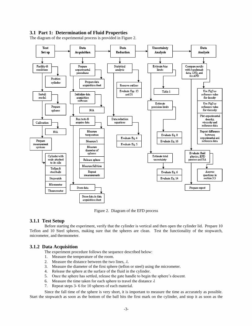
3.1 Part 1: Determination of Fluid Properties The diagram of the experimental process is provided in Figure 2.

Figure 2. Diagram of the EFD process

3.1.1 Test Setup Before starting the experiment, verify that the cylinder is vertical and then open the cylinder lid. Prepare 10

Teflon and 10 Steel spheres, making sure that the spheres are clean. Test the functionality of the stopwatch,

micrometer, and thermometer.

3.1.2 Data Acquisition The experiment procedure follows the sequence described below:

1. Measure the temperature of the room.

2. Measure the distance between the two lines, .

3. Measure the diameter of the first sphere (teflon or steel) using the micrometer.

4. Release the sphere at the surface of the fluid in the cylinder.

5. Once the sphere has settled, release the gate handle to begin the sphere’s descent.

6. Measure the time taken for each sphere to travel the distance

7. Repeat steps 3- 6 for 10 spheres of each material.

Since the fall time of the sphere is very short, it is important to measure the time as accurately as possible.

Start the stopwatch as soon as the bottom of the ball hits the first mark on the cylinder, and stop it as soon as the

-4-

bottom of the ball hits the second mark. Two people should cooperate in this measurement with one observing the

first mark and handling the stopwatch, and the other observing the second mark. A spreadsheet should be created for

data acquisition, following the example shown in Figure 3, below. The data from your spreadsheet will later be

inserted into Lab1_Data_Reduction_Sheet for data reduction and uncertainty analysis.

Figure 3. Sample data acquisition spreadsheet

3.1.3 Data Reduction

Figure 2 illustrates the block diagram of the measurement systems and data reduction equations for the

results. Use Lab1_Data_Reduction_Sheet for the data reduction procedure after importing the data from your

spreadsheet.

Data reduction includes the following steps:

1. Calculate the statistics (mean and standard deviations) of the repeated measurements.

2. Calculate the fluid density for each individual measurement using equation (5).

3. Calculate the kinematic viscosity for each individual measurement using equation (4).

3.1.4 Uncertainty Analysis

Uncertainties for the experimentally-determined glycerin

density and kinematic viscosity will be evaluated using

Lab1_Data_Reduction_Sheet. The methodology for

estimating uncertainties follows the AIAA S-071-1995

Standard (AIAA, 1995) as summarized in Stern et al.

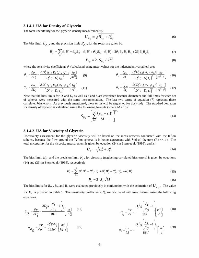
(1999), for multiple tests. Figure 4 is a block diagram

depicting error propagation methodology for the

measured density and viscosity. The data reduction

equations for density and viscosity of glycerin are

equations (5) and (4), respectively. Using these data

reduction equations, first, the elemental errors for each

independent variable, Xi, should be identified using the

best available information for bias errors, and using

repeated measurements for precision errors. Table 1

contains a summary of the elemental bias errors assumed

for the present experiment. For this investigation, we

will neglect the contribution of correlated bias errors.

Figure 4. Block diagram of the experiment, including

measurement systems, data reduction equations, and

results

Table 1. Assessment of the bias limits for the independent variables

Bias limit Bias Limit Estimation

BD= BDs = BDt 0.000005 m ½ instrument resolution

Bt = Bts = Btt 0.01 s Last significant digit

B 0.00079 m ½ instrument resolution

EXPERIMENTAL ERROR SOURCES

EXPERIMENTALRESULTS

X

B , P

SPHEREDIAMETER

FALLDISTANCE

FALLTIME

X

B , P

INDIVIDUALMEASUREMENT

SYSTEMS

MEASUREMENTOF INDIVIDUAL

VARIABLES

DATA REDUCTIONEQUATIONS

X

B , P

= (X , X ) =D t - D t

D t - D t

= (X , X , X , X ) =

D g( -1)t

18

B , P

B , P

D

D

DD

t

D t

t tt

2 2

2

2

2

tts s

s s s

sphere

s,t

s,t s,t

t

t

t

-5-

3.1.4.1 UA for Density of Glycerin

The total uncertainty for the glycerin density measurement is:

22

GGGPBU (6)

The bias limit G

B , and the precision limit G

P , for the result are given by:

tsttstttDstDsDtDststsDsDtttttDtDi

j

i

iGBBBBBBBBBB

22222222222

1

22

(7)

MSPGG

/2 (8)

where the sensitivity coefficients (calculated using mean values for the independent variables) are:

2

2 42 2t

sGD

t t t s

2 D ( - )t t D kgtt s s t

D mD t - D ts

(9)

2 2

2 32 2t

s tGt

t t t s s

D D ( - )t kgs s t t m sD t - D t

(10)

2

2 42 2s

tGD

s t t s

2 D ( - )t t D kgst s t s

D mD t - D ts

(11)

2 2

2 32 2

s tGts

s t t s s

D D ( - )t kgt t s t m sD t - D t

(12)

Note that the bias limits for Dt and Ds as well as tt and ts are correlated because diameters and fall times for each set

of spheres were measured with the same instrumentation. The last two terms of equation (7) represent these

correlated bias errors. As previously mentioned, these terms will be neglected for this study. The standard deviation

for density of glycerin is calculated using the following formula (where M = 10):

2/1

1

2

1

M

k

k

MS

G

(13)

3.1.4.2 UA for Viscosity of Glycerin

Uncertainty assessment for the glycerin viscosity will be based on the measurements conducted with the teflon

spheres, because the flow around the Teflon spheres is in better agreement with Stokes’ theorem (Re << 1). The

total uncertainty for the viscosity measurement is given by equation (24) in Stern et al. (1999), and is:

22

PBU (14)

The bias limit B , and the precision limit P , for viscosity (neglecting correlated bias errors) is given by equations

(14) and (23) in Stern et al. (1999), respectively:

222222222

1

22

BBBBBB

GGtttttDtDi

j

i

i

(15)

MSP 2 (16)

The bias limits for BDt , Btt, and B were evaluated previously in conjunction with the estimation of G

U . The value

for B is provided in Table 1. The sensitivity coefficients, i, are calculated with mean values, using the following

equations:

2 1

18

tD g tt t

mGD D st t

(17) 2

2

2 1

18t

tD gt

mGt t s

(18)

25

218

t t

G G

D g t mt

kg sG

(19)

2

2 1

18

ttD g t

tmG

s

(20)

-6-

Note that, unlike for density, there are no correlated bias errors contributing to the viscosity result, because only one

set of sphere measurements were used. The standard deviation for the viscosity of glycerin, for M=10 repeated

measurements, is calculated using the following formula:

2/1

1

2

1

M

k

k

MS

(21)

3.1.5 Data Analysis

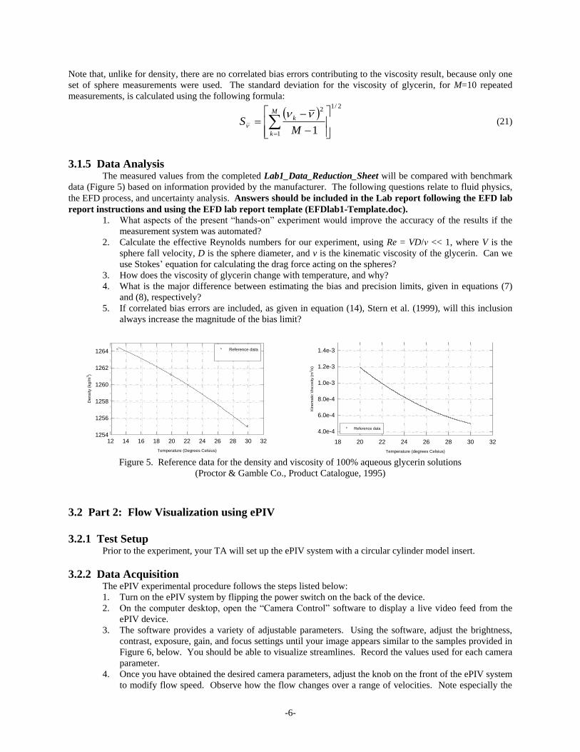
The measured values from the completed Lab1_Data_Reduction_Sheet will be compared with benchmark

data (Figure 5) based on information provided by the manufacturer. The following questions relate to fluid physics,

the EFD process, and uncertainty analysis. Answers should be included in the Lab report following the EFD lab

report instructions and using the EFD lab report template (EFDlab1-Template.doc).

1. What aspects of the present “hands-on” experiment would improve the accuracy of the results if the

measurement system was automated?

2. Calculate the effective Reynolds numbers for our experiment, using Re = VD/ν << 1, where V is the

sphere fall velocity, D is the sphere diameter, and v is the kinematic viscosity of the glycerin. Can we

use Stokes’ equation for calculating the drag force acting on the spheres?

3. How does the viscosity of glycerin change with temperature, and why?

4. What is the major difference between estimating the bias and precision limits, given in equations (7)

and (8), respectively?

5. If correlated bias errors are included, as given in equation (14), Stern et al. (1999), will this inclusion

always increase the magnitude of the bias limit?

Figure 5. Reference data for the density and viscosity of 100% aqueous glycerin solutions

(Proctor & Gamble Co., Product Catalogue, 1995)

3.2 Part 2: Flow Visualization using ePIV

3.2.1 Test Setup Prior to the experiment, your TA will set up the ePIV system with a circular cylinder model insert.

3.2.2 Data Acquisition The ePIV experimental procedure follows the steps listed below:

1. Turn on the ePIV system by flipping the power switch on the back of the device.

2. On the computer desktop, open the “Camera Control” software to display a live video feed from the

ePIV device.

3. The software provides a variety of adjustable parameters. Using the software, adjust the brightness,

contrast, exposure, gain, and focus settings until your image appears similar to the samples provided in

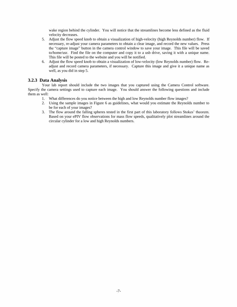
Figure 6, below. You should be able to visualize streamlines. Record the values used for each camera

parameter.

4. Once you have obtained the desired camera parameters, adjust the knob on the front of the ePIV system

to modify flow speed. Observe how the flow changes over a range of velocities. Note especially the

Temperature (Degrees Celsius)

12 14 16 18 20 22 24 26 28 30 32

De

nsity (

kg

/m3)

1254

1256

1258

1260

1262

1264 Reference data

Temperature (degrees Celsius)

18 20 22 24 26 28 30 32

Kin

em

atic V

isco

sity (

m2/s

)

4.0e-4

6.0e-4

8.0e-4

1.0e-3

1.2e-3

1.4e-3

Reference data

Temperature (Degrees Celsius)

12 14 16 18 20 22 24 26 28 30 32

Den

sity (

kg/m

3)

1254

1256

1258

1260

1262

1264 Reference data

Temperature (degrees Celsius)

18 20 22 24 26 28 30 32

Kin

em

atic V

isco

sity (

m2/s

)

4.0e-4

6.0e-4

8.0e-4

1.0e-3

1.2e-3

1.4e-3

Reference data

-7-

wake region behind the cylinder. You will notice that the streamlines become less defined as the fluid

velocity decreases.

5. Adjust the flow speed knob to obtain a visualization of high-velocity (high Reynolds number) flow. If

necessary, re-adjust your camera parameters to obtain a clear image, and record the new values. Press

the “capture image” button in the camera control window to save your image. This file will be saved

to/home/usr. Find the file on the computer and copy it to a usb drive, saving it with a unique name.

This file will be posted to the website and you will be notified.

6. Adjust the flow speed knob to obtain a visualization of low-velocity (low Reynolds number) flow. Re-

adjust and record camera parameters, if necessary. Capture this image and give it a unique name as

well, as you did in step 5.

3.2.3 Data Analysis Your lab report should include the two images that you captured using the Camera Control software.

Specify the camera settings used to capture each image. You should answer the following questions and include

them as well:

1. What differences do you notice between the high and low Reynolds number flow images?

2. Using the sample images in Figure 6 as guidelines, what would you estimate the Reynolds number to

be for each of your images?

3. The flow around the falling spheres tested in the first part of this laboratory follows Stokes’ theorem.

Based on your ePIV flow observations for mass flow speeds, qualitatively plot streamlines around the

circular cylinder for a low and high Reynolds numbers.

-8-

(a) Re = 90

(b) Re = 60

(c) Re = 30

(d) Re = 2

Figure 6. (a)-(d) Sample ePIV cylinder visualizations

4. References AIAA (1995). AIAA S-071-1995 Standard, American Institute of Aeronautics and Astronautics, Washington,

DC.

Batchelor, G.K. (1967). An Introduction to Fluid Dynamics, Cambridge University Press, London

Granger, R.A. (1988). Experiments in Fluid Mechanics, Holt, Rinehart and Winston, Inc. New York, NY

Proctor & Gamble Co., 1995, Product Catalogue.

Stern, F., Muste, M., Beninati, M-L, and Eichinger, W.E. (1999). “Summary of Experimental Uncertainty

Assessment Methodology with Example,” IIHR Report No. 406, The University of Iowa, Iowa City, IA.

White, F.M. (1994). Fluid Mechanics, 3rd edition, McGraw-Hill, Inc., New York, NY.

Visualization clips: http://css.engineering.uiowa.edu/fluidslab/referenc/concepts.html - Viscosity