EXECUTIVE SUMMARY RETURN OF THE QUANTS : … investment professionals only. Not for further...

For investment professionals only. Not for further distribution.

EXECUTIVE SUMMARY RETURN OF THE QUANTS: RISK BASED INVESTING

DECEMBER 2016

Anna Dreyer, Vice President Robert L. Harlow, Vice President

Stefan Hubrich, Vice President, Director of Asset Allocation Research

Sébastien Page, Co-Head of Asset Allocation

• Market volatility has increased in recent years. In the six decades after World War II, there were, on

average no more than three “tail events” per year. Between 2000 and 2010, the average has risen to an unprecedented nine three-sigma days per year.

• Volatility—and hence exposure to loss—is not stable through time. From 1994 to 2016, the rolling

one-year standard deviation for a 60/40 portfolio ranged from a low of less than 5% to a high of 20%. So a 60/40 portfolio is not always appropriate for a relatively risk-averse investor.

• A managed volatility strategy, by trading stock and bond futures, may adjust a 60/40 portfolio’s

exposure to stocks all the way down to 20% when markets are highly volatile and all the way up to 75% when markets are stable.

• This strategy is portable and can easily be applied as an overlay for almost any portfolio. Managed

volatility has been shown in practice to reduce exposure to loss and smooth the ride for investors, at a very low—or even positive—cost in terms of returns.

• While managed volatility is used mostly to reduce exposure to loss, we can think of covered call

writing as the other side of the coin for risk-based investing, in that investors use it mostly to generate excess returns.

• Covered call writing gives exposure to the volatility risk premium—which represents compensation

for providing insurance to market participants. • Research suggests that the volatility risk premium, which is absent from most investors’ portfolios,

has had more than double the risk-adjusted returns (Sharpe ratio) of the equity risk premium. • Managed volatility and covered call writing are negatively correlated. Therefore, combining these

risk-based investment tools may improve investment performance over time, especially when added to traditional equity or multi-asset portfolios.

• Despite our industry’s obsession with return forecasting, these two investment strategies focus on

risk. They do not require bold predictions on the direction of markets.

© 2016 CFA Institute. All rights reserved. • cfapubs.org Third Quarter 2016 • 1

Return of the Quants: Risk-Based InvestingAnna Dreyer, CFA Vice President, T. Rowe Price Baltimore

Robert L. Harlow, CFA Vice President, T. Rowe Price Baltimore

Stefan Hubrich, CFA Vice President, Director of Asset Allocation Research, T. Rowe Price Baltimore

Sébastien Page, CFACo-Head of Asset Allocation, T. Rowe Price Baltimore

Managed volatility and covered call writing are two of the few systematic investment strategies that have been shown to perform well across a variety of empirical studies and in practice. So far, they have been studied mostly as separate strategies. It turns out that when combined, these two strategies create a powerful toolset for portfolio enhancements.

The financial services industry is obsessed with return forecasting. Asset owners, investment

managers, sell-side strategists, and financial media pundits—all invest considerable time and resources to predict the direction of markets. Yet, risk-based investing may provide easier and more robust ways to improve portfolio performance, often without requiring return forecasting skill.

We will present two strategies that demonstrate the value of risk-based investing:1. Managed volatility2. Covered call writing

We will show that these strategies are nega-tively correlated. Therefore, they perform better together than as standalone portfolio enhance-ments. Such an integrated approach can improve the risk-adjusted performance of buy-and-hold

portfolios and provide a powerful toolset to bet-ter meet investor goals.1 We will also present the literature that supports

these strategies and discuss the corroborating data.

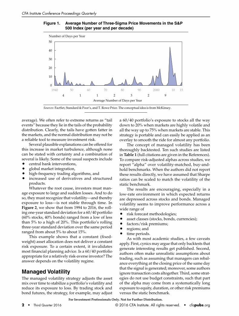
Increased VolatilityMarket volatility has increased in recent years. In Figure 1, we show that during the decade of the 1940s, on average, there were four days per year during which stocks moved by three standard devia-tions or more (“three-sigma days”).2 WWII created a lot of this turbulence. In the following six decades, the average rose no higher than three days per year. But recently, between 2000 and 2010, the average has risen to nine three-sigma days per year—more than any time in our long dataset.

According to the normal distribution, a three-sigma day should occur only 0.6 times per year (on

1Throughout the presentation, we assume that “buy-and-hold” portfolios maintain static weights over time. Therefore, strictly speaking, these portfolios or strategies are not entirely buy-and-hold, because they rebalance to target weights, either on a regular calendar basis (such as monthly) or when large deviations occur. 2Standard deviation is measured over the full sample of data.

Note: Sébastien Page, CFA, presented these remarks at the 69th CFA Institute Annual Conference. The authors would like to thank David Clewell, CFA, JJ Mignon, Charles Shriver, CFA, and Toby Thompson, CFA, for their contributions to this presentation, as well as Rich Whitney, CFA, for overseeing and supporting the development of these ideas.

This presentation comes from the 69th CFA Institute Annual Conference held in Montréal on 8–11 May 2016 in partnership with CFA Montréal.

For Investment Professionals Only. Not for Further Distribution.

CFA Institute Conference Proceedings Quarterly

2 • Third Quarter 2016 © 2016 CFA Institute. All rights reserved. • cfapubs.org

average). We often refer to extreme returns as “tail events” because they lie in the tails of the probability distribution. Clearly, the tails have gotten fatter in the markets, and the normal distribution may not be a reliable tool to measure investment risk.

Several plausible explanations can be offered for this increase in market turbulence, although none can be stated with certainty and a combination of several is likely. Some of the usual suspects include• central bank interventions,• global market integration,• high-frequency trading algorithms, and• increased use of derivatives and structured

products.Whatever the root cause, investors must man-

age exposure to large and sudden losses. And to do so, they must recognize that volatility—and thereby exposure to loss—is not stable through time. In Figure 2, we show that from 1994 to 2016, the roll-ing one-year standard deviation for a 60/40 portfolio (60% stocks, 40% bonds) ranged from a low of less than 5% to a high of 20%. This portfolio’s rolling three-year standard deviation over the same period ranged from about 5% to about 15%.

This example shows that a constant (fixed-weight) asset allocation does not deliver a constant risk exposure. To a certain extent, it invalidates most financial planning advice. Is a 60/40 portfolio appropriate for a relatively risk-averse investor? The answer depends on the volatility regime.

Managed VolatilityThe managed volatility strategy adjusts the asset mix over time to stabilize a portfolio’s volatility and reduce its exposure to loss. By trading stock and bond futures, the strategy, for example, may adjust

a 60/40 portfolio’s exposure to stocks all the way down to 20% when markets are highly volatile and all the way up to 75% when markets are stable. This strategy is portable and can easily be applied as an overlay to smooth the ride for almost any portfolio.

The concept of managed volatility has been thoroughly backtested. Ten such studies are listed in Table 1 (full citations are given in the References). To compare risk-adjusted alphas across studies, we report “alpha” over volatility-matched, buy-and-hold benchmarks. When the authors did not report these results directly, we have assumed that Sharpe ratios can be scaled to match the volatility of the static benchmark.

The results are encouraging, especially in a low-rate environment in which expected returns are depressed across stocks and bonds. Managed volatility seems to improve performance across a wide range of • risk forecast methodologies;• asset classes (stocks, bonds, currencies);• factors/risk premiums;• regions; and• time periods.

As with most academic studies, a few caveatsapply. First, cynics may argue that only backtests that generate interesting results get published. Second, authors often make unrealistic assumptions about trading, such as assuming that managers can rebal-ance everything at the closing price of the same day that the signal is generated; moreover, some authors ignore transaction costs altogether. Third, some strat-egies do not use budget constraints, such that part of the alpha may come from a systematically long exposure to equity, duration, or other risk premiums versus the static benchmark.

Figure 1. Average Number of Three-Sigma Price Movements in the S&P 500 Index (per year and per decade)

Number of Days per Year

50

40

30

20

10

01940 156050 80 2000 1070 90

2114 3 2 9

Average Number of Days per Year

Sources: FactSet, Standard & Poor’s, and T. Rowe Price. The conceptual idea is from McKinsey.


Return of the Quants


Figure 2. Rolling One- and Three-Year Volatilities for a 60/40 Portfolio

Note: The balanced strategy is 60% S&P 500 Index and 40% Bloomberg Barclays US Aggregate Index rebalanced monthly. Sources: Ibbotson Associates, Standard & Poor’s, and Barclays.

Table 1. Selected Studies on Managed Volatility

Year Study Backtest Volatility Forecast Universe Period Alpha (%)

2001 Fleming, Kirby, and Ostdiek

Daily, MVO Nonparametric daily 4 asset classes 1983–1997 1.5

2003 Fleming, Kirby, and Ostdiek

Daily, MVO Nonparametric, intraday 4 asset classes 1984–2000 2.8

2011 Kritzman, Li, Page, and Rigobon

Daily Absorption ratio 6 countries 1998–2010 4.5

2012 Kritzman, Page, and Turkington

Monthly, TAA Regime-switching 15 risk premiums 1978–2009 2.5

2012 Hallerbach Daily Trailing six-months daily EURO STOXX 50 vs. cash

2003–2011 2.2

2013 Kritzman Daily, TAA Absorption ratio 8 asset classes 1998–2013 4.9

2013 Dopfel and Ramkumar Quarterly Regime-switching S&P 500 vs. cash 1950–2011 2.0

2013 Hocquard, Ng, and Papageorgiou

Daily GARCH 7 asset classes 1990–2011 2.6

2014 Perchet, Carvalho, and Moulin

Daily GARCH 22 factors 1980–2013 3.0

2016 Moreira and Muir Monthly Trailing one-month daily 10 factors, 20 countries

1926–2015 3.5

Notes: We report the average of key results or the key results as reported by the authors. MVO refers to mean–variance optimization; TAA refers to various multi-asset portfolio shifts; all other backtests involve timing exposure to a single market or risk premiums. Countries refers to country equity markets, except for Perchet, Carvalho, and Moulin (2014), which includes value and momentum factors across 10 countries and 10 currencies. Some backtests in Fleming, Kirby, and Ostdiek (2001) and Perchet, Carvalho, and Moulin (2014) involve shorter time series because of the lack of available data. The backtest by Dopfel and Ramkumar (2013) is in-sample. The regime-switching model in Kritzman, Page, and Turkington (2012) combines turbulence, GDP, and inflation regimes. Readers should refer to the original papers for more information on the volatility forecast methodologies. Regarding transaction costs, Fleming, Kirby, and Ostdiek (2001, 2003) assume execution via futures contracts and estimate transaction costs in the 10–20 bps range. Moreira and Muir (2016) report transaction costs in the 56–183 bps range for physicals. All other studies do not report transaction costs.




Nonetheless, although these risk-adjusted alphas should be shaved to account for the usual implementation shortfall between backtests and real-ity, managed volatility has been shown in practice to reduce exposure to loss and smooth the ride for investors, at a very low—or even positive—cost in terms of returns.

Managed Volatility Model Portfolio. Consider a backtest that we have built specifically to represent real-world implementation. For this example, we set a target of 11% volatility for a balanced portfolio of 65% stocks and 35% bonds. We scaled the overlay to avoid any systematically long equity or duration exposure versus the underlying portfolio. We allowed the man-aged volatility overlay to reduce equity exposure to as low as 20% and increase it as high as 75%.3

We then applied a band of 14% and 10% volatil-ity around the target. As long as volatility remained within the band, no rebalancing was required. When volatility rose above or fell below the bands, the strategy rebalanced the overlay to meet the (expected) volatility target. We used a wider upper band because volatility tends to spike up a lot more than it tends to spike down, so the asymmetrical bands are meant to reduce noise and minimize the intrusiveness of the algorithm.

Within the portfolio, we assumed that 95% of assets were invested directly in a balanced strategy composed of actively managed mandates (i.e., within each of the asset classes, managers engaged in security selection).4 The remaining 5% were set aside as the cash collateral for the volatility management overlay, which we assumed to be invested in Treasury bills. When volatility was at target, the futures overlay was set to match the balanced portfolio at 65% stocks and 35% bonds. Equity futures were allocated 70% to the S&P 500 Index and 30% to the MSCI EAFE (Europe, Australasia, and the Far East) Index futures, to reflect the neutral US/non-US equity mix inside the bal-anced strategy. Lastly, we imposed a minimum daily trade size of 1% and maximum trade size of 10% of the portfolio’s notional.

To forecast volatility, we used a DCC–EGARCH model (dynamic conditional correlation, expo-nentially weighted generalized autoregressive conditional heteroskedasticity) with fat-tailed dis-tributions. This model replicates fairly closely the implied volatility on traded options and thus how investors in general forecast volatility. DCC relates

3Notice that the model allows for adding risk above the 65% strate-gic allocation when volatility is low. In fact, investors can calibrate managed volatility overlays to any desired risk level, including levels above the underlying portfolio’s static exposure. 4Note that we used an actual track record for an actively man-aged balanced fund. However, this example is for illustrative purposes only.

to time-varying correlations, and the ARCH category of models accounts for the time-series properties of volatility, such as its persistence or tendency to clus-ter. We re-estimated the model daily using 10 years of data ending the day prior to forecast.5 Volatility forecasts were updated daily using the most current parameter estimates. Importantly, we strictly used information known at the time to determine how to trade the overlay.

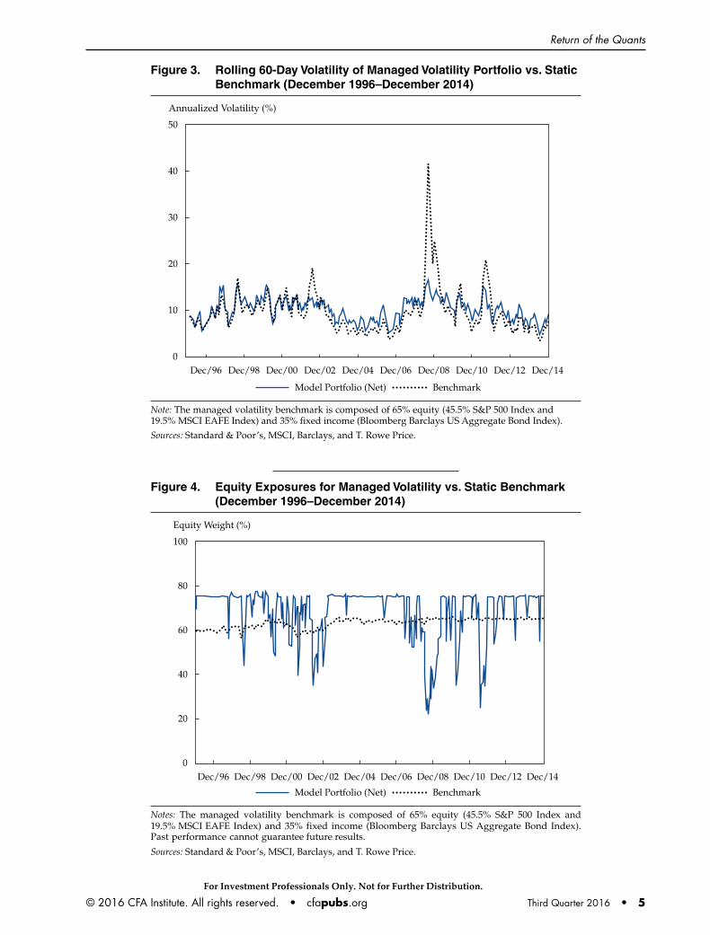
In Figure 3, we show the rolling volatility for the strategy versus a static benchmark.6

As expected, over the 18-year period studied, managed volatility has consistently stabilized real-ized volatility compared with a static benchmark—despite the relatively wide bands used in our algo-rithm and despite the fact that volatility is measured on a very short window of 60 days (shorter windows tend to show more variability in volatility). The algo-rithm worked particularly well during the 2008–09 financial crisis.

In Figure 4, we show the strategy’s equity expo-sure during the same 18-year period. The strategy is quite tactical. Although it does not trade more than 10% of the portfolio’s notional value in futures in a given day, some of the shifts in equity allocations are meaningful and occur over relatively short periods of time.

In Figure 5, we show the realized annualized return and worst drawdown for three balanced fund strategies:• “Balanced portfolio with active components” is

the static balanced fund that allocates to actively managed building blocks.

• “Balanced portfolio with active components and MVOL” is the same balanced fund with active building blocks, to which we have applied the managed volatility overlay on the entire notional.

• “Balanced portfolio with index components” is the static balanced fund allocated to passive (index) building blocks.We also show results for US bonds, US stocks

(S&P 500), and international stocks (MSCI EAFE).

In this example, active managers added returns over passive benchmarks (after fees) through secu-rity selection while slightly increasing exposure to loss. When we applied the managed volatility over-lay to this portfolio, we sacrificed a few basis points of returns, but we significantly reduced drawdown exposure.

5We used an expanding window, increasing from 3 years to 10 years, until 10 years of data became available.6Here the benchmark (static portfolio) is invested in passive (index) building blocks. The portfolio with actively managed building blocks generated similar results for the purposes of this illustration.




Figure 4. Equity Exposures for Managed Volatility vs. Static Benchmark (December 1996–December 2014)

Equity Weight (%)

100

80

60

40

20

0Dec/14Dec/00Dec/98 Dec/02 Dec/06 Dec/10Dec/96 Dec/04 Dec/08 Dec/12

Model Portfolio (Net) Benchmark

Notes: The managed volatility benchmark is composed of 65% equity (45.5% S&P 500 Index and19.5% MSCI EAFE Index) and 35% fixed income (Bloomberg Barclays US Aggregate Bond Index).Past performance cannot guarantee future results.

Sources: Standard & Poor’s, MSCI, Barclays, and T. Rowe Price.

Figure 3. Rolling 60-Day Volatility of Managed Volatility Portfolio vs. Static Benchmark (December 1996–December 2014)

Annualized Volatility (%)

50

40

30

20

10

0Dec/14Dec/00 Dec/02 Dec/06 Dec/08 Dec/12Dec/98Dec/96 Dec/04 Dec/10

Model Portfolio (Net) Benchmark

Note: The managed volatility benchmark is composed of 65% equity (45.5% S&P 500 Index and19.5% MSCI EAFE Index) and 35% fixed income (Bloomberg Barclays US Aggregate Bond Index).

Sources: Standard & Poor’s, MSCI, Barclays, and T. Rowe Price.




Why Would Managed Volatility Improve Risk-Adjusted Return? To explain this success, we must understand why volatility is persistent (and therefore predictable). Periods of low and high vola-tility—so-called risk regimes—tend to persist for a while. This persistence is crucial to the success of the strategy, and it means that simple volatility forecasts can be used to adjust risk exposures.

A fundamental argument could be made that shocks to the business cycle themselves tend to clus-ter. Bad news often follows bad news. The use of leverage—in financial markets and in the broader economy—may also contribute to volatility cluster-ing. Leverage often takes time to unwind. Other explanations may be related to behavioral aspects of investing that are common to investors across mar-kets, such as “fear contagion,” extrapolation biases, and the financial media’s overall negativity bias.

In terms of managing tail risk specifically, one way to explain how managed volatility works is to represent portfolio returns as being generated by a mixture of distributions, which is consistent with the concept of risk regimes. When we mix high-volatility and low-volatility distributions and randomly draw from either, we get a fat-tailed distribution. By adjust-ing risk exposures, managed volatility essentially

“normalizes” portfolio returns to one single distribu-tion and thereby significantly reduces tail risk.

Importantly, short-term expected (or “forward”) returns do not seem to increase after volatility spikes, which explains why managed volatility often out-performs buy-and-hold in terms of Sharpe ratio (or risk-adjusted performance in general). This phenom-enon has been studied in academia (see, for example, Moreira and Muir 2016). Most explanations focus on the time horizon mismatch between managed vola-tility and value investing. Moreira and Muir (2016) observe that expected returns adjust more slowly than volatility. Therefore, managed volatility strategies may re-risk the portfolio when market turbulence has subsided and still capture the upside from attractive valuations. The performance of managed volatility around the 2008 crisis is a good example. As Moreira and Muir (2016) put it:

Our [managed volatility] portfolios reduce risk taking during these bad times—times when the common advice is to increase or hold risk taking constant. For example, in the aftermath of the sharp price declines in the fall of 2008, it was a widely held view that those that reduced positions in equities were missing a once-in-a-generation buying

Figure 5. Simulated Risk–Return Profile of Managed Volatility Models and Market Indexes (January 1996–December 2014)

Annualized Return (%)

9

8

7

6

5

4

3

2

1

00 6010 20 30 40 50

Drawdown (%)

MSCI EAFE

Balanced Portfolio with Index Components

S&P 500

Balanced Portfolio with Active Components

Balanced Portfolio with Active Components and MVOL

Bloomberg Barclays US Aggregate

Notes: Example for illustrative purposes only. The results above are hypothetical and do not represent the returns of any T. Rowe Price product or strategy. The results of the Balanced Portfolios are shown net of a hypothetical management fee of (37.5 bps). Sources: Standard & Poor’s, MSCI, Barclays, and T. Rowe Price.




opportunity. Yet our strategy cashed out almost completely and returned to the mar-ket only as the spike in volatility receded . . . . Our simple strategy turned out to work well throughout several crisis episodes, including the Great Depression, the Great Recession, and the 1987 stock market crash. (p. 2)

Another way of thinking about how managed volatility may increase Sharpe ratios in certain mar-ket environments is to think of time diversification as being similar to cross-sectional diversification. Suppose we invest in five different stocks with the same Sharpe ratios but very different volatility levels. If we assume the stocks are uncorrelated, we should allocate equal risk (not equal value weights) to get the Sharpe ratio–maximizing portfolio. The same logic applies through time; the realized variance of the portfolio is basically the sum of the point-in-time variances. So, to get the highest Sharpe ratio through time, we should allocate equal risk to each period.

However, managed volatility does not always outperform static portfolios. For example, when spikes in volatility are followed by short-term return gains, managed volatility may miss out on those gains (versus a buy-and-hold portfolio). Also, it is possible for large market drawdowns to occur when volatility is very low. In those situations, managed volatility strategies that overweight stocks in quiet times (to a higher weight than the static portfolio) may underperform.

In sum, the empirical observations in support of managed volatility—volatility persistence and the lack of correlation between volatility spikes and short-term forward returns—hold on average but not in all market environments.

Covered Call Writing (Volatility Risk Premium)Although managed volatility is used mostly to reduce exposure to loss, we can think of covered call writing as the other side of the coin for risk-based investing, in that investors use it mostly to generate excess returns. The basics of the strategy are simple: The investor sells a call option and simultaneously buys the underlying security or index. Covered call writing gives expo-sure to the volatility risk premium, one of the best performing of the “alternative betas” that have risen in popularity recently. As mentioned by Israelov and Nielsen (2015), “The volatility risk premium, which is absent from most investors’ portfolios, has had more than double the risk-adjusted returns (Sharpe ratio) of the equity risk premium” (p. 44).

In the same article, the authors decompose the return from covered call writing into three components:

1. The equity risk premium, net of the call delta or“equity sensitivity exposure”7

2. The volatility risk premium, which is the difference between implied volatility from option pricesand realized volatility

3. A dynamic equity exposure, which is a reversalcomponent that exists if investors do not delta-hedge their equity exposure over time

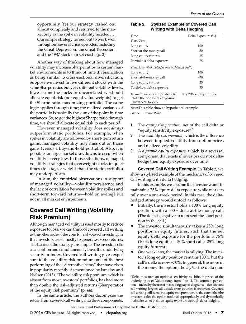
Covered Call Writing Example. In Table 2, weshow a stylized example of the mechanics of covered call writing with delta hedging.

In this example, we assume the investor wants to maintain a 75% equity delta exposure while markets rally over a one-week period. In this case, the delta-hedged strategy would unfold as follows:• Initially, the investor holds a 100% long equity

position, with a –50% delta at-the-money call.(The delta is negative to represent the short posi-tion in the call.)

• The investor simultaneously takes a 25% longposition in equity futures, such that the netequity delta exposure for the portfolio is 75%(100% long equities – 50% short call + 25% longequity futures).

• One week later, the market is rallying. The inves-tor’s long equity position remains 100%, but the call’s delta is now –70%. In general, the more inthe money the option, the higher the delta (and

7Delta measures an option’s sensitivity to shifts in prices of the underlying asset. Values range from –1 to +1. The common percep-tion—fueled by the use of misleading payoff diagrams—that covered call writing forgoes all upside from equities is incorrect. Covered call writing still earns the equity risk premium, to the extent that the investor scales the option notional appropriately and dynamically maintains a net positive equity exposure through delta hedging.

Table 2. Stylized Example of Covered Call Writing with Delta Hedging

Time Delta Exposure (%)Time: Zero

Long equity 100

Short at-the-money call –50

Long equity futures 25

Portfolio’s delta exposure 75

Time: One Week Later/Scenario: Market Rally

Long equity 100

Short at-the-money call –70

Long equity futures 25

Portfolio’s delta exposure 55

To maintain a portfolio delta to take the portfolio’s exposure from 55% to 75%

Buy 20% equity futures

Note: This table shows a hypothetical example.

Source: T. Rowe Price.




ipso facto, the more negative the delta on the short position).

• The long equity futures remains 25%. Therefore, the portfolio’s delta exposure is down to 55%(100% long equity – 70% short call + 25% longequity futures).

• To maintain a portfolio delta of 75%, the investor buys 20% in equity futures.This example shows how delta hedging works:

The investor estimates the equity sensitivity of the call at any point in time (or according to some prede-termined frequency) and adjusts the portfolio to its targeted net equity exposure using futures. Doing so isolates the volatility risk premium and negates the dynamic equity exposure/reversal timing compo-nent of covered call writing.8 As Israelov and Nielsen (2015) show, this component tends to detract from the performance of covered call writing—hence delta hedging tends to add value.

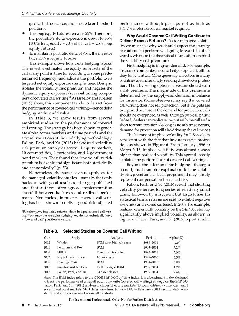
In Table 3, we show results from several empirical studies on the performance of covered call writing. The strategy has been shown to gener-ate alpha across markets and time periods and for several variations of the underlying methodology. Fallon, Park, and Yu (2015) backtested volatility risk premium strategies across 11 equity markets, 10 commodities, 9 currencies, and 4 government bond markets. They found that “the volatility risk premium is sizable and significant, both statistically and economically” (p. 53).

Nonetheless, the same caveats apply as for the managed volatility studies—namely, that only backtests with good results tend to get published and that authors often ignore implementation shortfall between backtests and realized perfor-mance. Nonetheless, in practice, covered call writ-ing has been shown to deliver good risk-adjusted

8For clarity, we implicitly refer to “delta-hedged covered call writ-ing,” but once we are delta hedging, we do not technically have a “covered call” position anymore.

performance, although perhaps not as high as 6%–7% alpha across all market regimes.

Why Would Covered Call Writing Continue to Deliver Excess Returns? As for managed volatil-ity, we must ask why we should expect the strategy to continue to perform well going forward. In other words, what are the theoretical foundations behind the volatility risk premium?

First, hedging is in great demand. For example, insurance companies need to hedge explicit liabilities they have written. More generally, investors in many countries are increasingly seeking drawdown protec-tion. Thus, by selling options, investors should earn a risk premium. The magnitude of this premium is determined by the supply-and-demand imbalance for insurance. (Some observers may say that covered call writing does not sell protection. But if the puts are overpriced because of the demand for protection, calls should be overpriced as well, through put–call parity. Indeed, dealers can replicate the put with the call and a short forward position. As long as no arbitrage occurs, demand for protection will also drive up the call price.)

The history of implied volatility for US stocks is consistent with the fact that investors crave protec-tion, as shown in Figure 6. From January 1996 to March 2016, implied volatility was almost always higher than realized volatility. This spread loosely explains the performance of covered call writing.

Beyond the “demand for hedging” theory, a second, much simpler explanation for the volatil-ity risk premium has been proposed: It may simply represent compensation for its tail risk.

Fallon, Park, and Yu (2015) report that shorting volatility generates long series of relatively small gains, followed by infrequent but large losses (in statistical terms, returns are said to exhibit negative skewness and excess kurtosis). In 2008, for example, realized one-month volatility on the S&P 500 shot up significantly above implied volatility, as shown in Figure 6. Fallon, Park, and Yu (2015) report similar

Table 3. Selected Studies on Covered Call Writing

Year Study Analysis Period Alpha (%)

2002 BXM with bid–ask costs 1988–2001 6.2%2005 BXM 2003–2004 5.2%2006 Dynamic strategies 1990–2005 7.0%2007 10 backtests 1996–2006 3.5%2008 BXM 1988–2005 5.8%2015 Delta-hedged BXM 1996–2014 1.7%2015

WhaleyFeldman and Roy

Hill et al.Kapadia and Szado

Ilya Figelman

Israelov and Nielsen Fallon, Park, and Yu 34 asset classes 1995–2014 2.4%

Notes: The BXM index refers to the CBOE S&P 500 BuyWrite Index. It is a benchmark index designed to track the performance of a hypothetical buy-write (covered call writing) strategy on the S&P 500. Fallon, Park, and Yu’s (2015) analysis includes 11 equity markets, 10 commodities, 9 currencies, and 4 government bond markets. Start dates vary from January 1995 to February 2001 based on data avail-ability, and alpha is averaged across all backtests.




tail risks in the volatility risk premium for 33 out of 34 of the asset classes they studied.

Both explanations—the demand for hedging and the compensation for tail risk—are, in fact, connected. Providers of insurance should expect negatively skewed returns, by definition. The bottom line is that if long-term investors can accept negative skewness in their returns, they should get compensa-tion through the volatility risk premium.

Combining Managed Volatility and Covered Call WritingInvestors can use managed volatility to reduce the tail risk exposure in covered call writing. In general, investors should think of risk-based investing as a set of tools, rather than standalone strategies. Low or even negative correlations between risk-based investing strategies can add a lot of value to a port-folio, even when the individual strategies’ Sharpe ratios are relatively low.

In Table 4, we show the correlation of monthly returns above cash from January 1996 to December 2015 for (1) the S&P 500, (2) covered call writing, and (3) managed volatility (overlay only, without the equity exposure). In this case, the covered call writing strategy sells at-the-money calls and main-tains an equity delta of 0. The managed volatility strategy captures the excess return above the S&P 500 by increasing and decreasing exposure to stocks based on market volatility. The strategy

• buys stocks’ futures when short-term trailingvolatility is lower than long-term volatility and

• sells stocks’ futures when the short-term volatil-ity is higher than long-term volatility.We calculated short-term realized volatility on a

60-day rolling window. For long-term volatility, weused an expanding window of out-of-sample datagoing back to January 1940.

The correlation between the S&P 500 and cov-ered call writing was 36%—a very low number for a risk premium (hence the term “alternative” beta).9 Between the S&P 500 and managed volatility, the correlation was –51%. In this case, a strong nega-tive correlation was expected because, by defini-tion, managed volatility aims to reduce exposure to loss. Importantly, the correlation between managed

9However, this correlation may increase in times of market stress.

Figure 6. Implied Market Volatility Compared with Realized Market Volatility (January 1990–March 2016)

Percent

90

80

70

60

50

40

30

20

10

01990 95 2000 05 10 15

Implied Realized

Notes: The VIX represents investors’ expectations of the S&P 500 Index’s volatility over the next 30-day period. Data are as of March 2016.

Sources: S&P 500, Bloomberg, and T. Rowe Price.

Table 4. Correlations across Strategies and the S&P 500 (January 1996–December 2015)

Monthly Returns above Cash Covered Calls Managed Volatility

Managed volatility –0.20

S&P 500 0.36 –0.51

Notes: All returns are excess of cash, which is defined as the total return of three-month US Treasury bills. The data exclude the impact of fees and trading costs.

Sources: T. Rowe Price, Ibbotson Associates, OptionMetrics, and Standard & Poor’s.




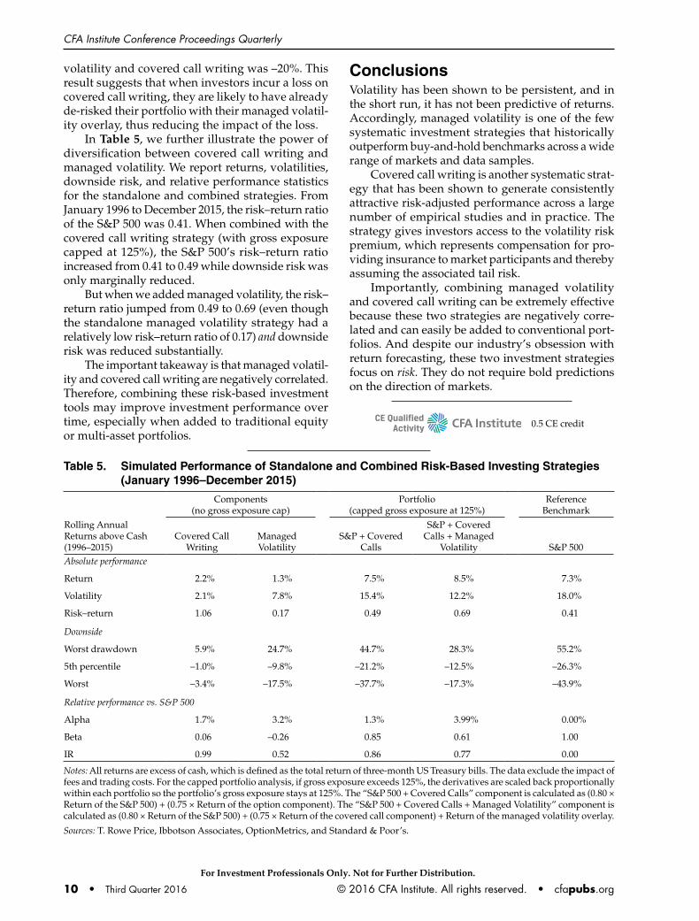
volatility and covered call writing was –20%. This result suggests that when investors incur a loss on covered call writing, they are likely to have already de-risked their portfolio with their managed volatil-ity overlay, thus reducing the impact of the loss.

In Table 5, we further illustrate the power of diversification between covered call writing and managed volatility. We report returns, volatilities, downside risk, and relative performance statistics for the standalone and combined strategies. From January 1996 to December 2015, the risk–return ratio of the S&P 500 was 0.41. When combined with the covered call writing strategy (with gross exposure capped at 125%), the S&P 500’s risk–return ratio increased from 0.41 to 0.49 while downside risk was only marginally reduced.

But when we added managed volatility, the risk–return ratio jumped from 0.49 to 0.69 (even though the standalone managed volatility strategy had a relatively low risk–return ratio of 0.17) and downside risk was reduced substantially.

The important takeaway is that managed volatil-ity and covered call writing are negatively correlated. Therefore, combining these risk-based investment tools may improve investment performance over time, especially when added to traditional equity or multi-asset portfolios.

ConclusionsVolatility has been shown to be persistent, and in the short run, it has not been predictive of returns. Accordingly, managed volatility is one of the few systematic investment strategies that historically outperform buy-and-hold benchmarks across a wide range of markets and data samples.

Covered call writing is another systematic strat-egy that has been shown to generate consistently attractive risk-adjusted performance across a large number of empirical studies and in practice. The strategy gives investors access to the volatility risk premium, which represents compensation for pro-viding insurance to market participants and thereby assuming the associated tail risk.

Importantly, combining managed volatility and covered call writing can be extremely effective because these two strategies are negatively corre-lated and can easily be added to conventional port-folios. And despite our industry’s obsession with return forecasting, these two investment strategies focus on risk. They do not require bold predictions on the direction of markets.

CE QualifiedActivity 0.5 CE credit

Table 5. Simulated Performance of Standalone and Combined Risk-Based Investing Strategies (January 1996–December 2015)

Components (no gross exposure cap)

Portfolio (capped gross exposure at 125%)

Reference Benchmark

Rolling Annual Returns above Cash (1996–2015)

Covered Call Writing

Managed Volatility

S&P + Covered Calls

S&P + Covered Calls + Managed

Volatility S&P 500Absolute performance

Return 2.2% 1.3% 7.5% 8.5% 7.3%

Volatility 2.1% 7.8% 15.4% 12.2% 18.0%

Risk–return 1.06 0.17 0.49 0.69 0.41

Downside

Worst drawdown 5.9% 24.7% 44.7% 28.3% 55.2%

5th percentile –1.0% –9.8% –21.2% –12.5% –26.3%

Worst –3.4% –17.5% –37.7% –17.3% –43.9%

Relative performance vs. S&P 500

Alpha 1.7% 3.2% 1.3% 3.99% 0.00%

Beta 0.06 –0.26 0.85 0.61 1.00

IR 0.99 0.52 0.86 0.77 0.00

Notes: All returns are excess of cash, which is defined as the total return of three-month US Treasury bills. The data exclude the impact of fees and trading costs. For the capped portfolio analysis, if gross exposure exceeds 125%, the derivatives are scaled back proportionally within each portfolio so the portfolio’s gross exposure stays at 125%. The “S&P 500 + Covered Calls” component is calculated as (0.80 × Return of the S&P 500) + (0.75 × Return of the option component). The “S&P 500 + Covered Calls + Managed Volatility” component is calculated as (0.80 × Return of the S&P 500) + (0.75 × Return of the covered call component) + Return of the managed volatility overlay.

Sources: T. Rowe Price, Ibbotson Associates, OptionMetrics, and Standard & Poor’s.




RefeRences

Dopfel, Frederick E., and Sunder R. Ramkumar. 2013. “Managed Volatility Strategies: Applications to Investment Policy.” Journal of Portfolio Management, vol. 40, no. 1 (Fall): 27–39.

Fallon, William, James Park, and Danny Yu. 2015. “Asset Allocation Implications of the Global Volatility Premium.” Financial Analysts Journal, vol. 71, no. 5 (September/October): 38–56.

Feldman, Barry E., and Dhruv Roy. 2005. “Passive Options-Based Investment Strategies: The Case of the CBOE S&P 500 Buy Write Index.” Journal of Investing, vol. 2004, no. 1 (Fall): 72–89.

Figelman, Ilya. 2008. “Expected Return and Risk of Covered Call Strategies.” Journal of Portfolio Management, vol. 34, no. 4 (Summer): 81–97.

Fleming, Jeff, Chris Kirby, and Barbara Ostdiek. 2001. “The Economic Value of Volatility Timing.” Journal of Finance, vol. 56, no. 1 (February): 329–352.

———. 2003. “The Economic Value of Volatility Timing Using ‘Realized’ Volatility.” Journal of Financial Economics, vol. 67, no. 3 (March): 473–509.

Hallerbach, Winfried G. 2012. “A Proof of the Optimality of Volatility Weighting Over Time.” Working paper (28 May): http://papers.ssrn.com/sol3/papers.cfm?abstract_id=2008176.

Hill, Joanne M., Venkatesh Balasubramanian, Krag (Buzz) Gregory, and Ingrid Tierens. 2006. “Finding Alpha via Covered Index Writing.” Financial Analysts Journal, vol. 62, no. 5 (September/October): 29–46.

Hocquard, Alexandre, Sunny Ng, and Nicolas Papageorgiou. 2013. “A Constant-Volatility Framework for Managing Tail Risk.” Journal of Portfolio Management, vol. 39, no. 2 (Winter): 28–40.

Israelov, Roni, and Lars N. Nielsen. 2015. “Covered Calls Uncovered.” Financial Analysts Journal, vol. 71, no. 6 (November/December): 44–57.

Kapadia, Nikunj, and Edward Szado. 2007. “The Risk and Return Characteristics of the Buy-Write Strategy on the Russell 2000 Index.” Journal of Alternative Investments, vol. 9, no. 4 (Spring): 39–56.

Kritzman, Mark. 2013. “Risk Disparity.” Journal of Portfolio Management, vol. 40, no. 1 (Fall): 40–48.

Kritzman, Mark, Yuanzhen Li, Sébastien Page, and Roberto Rigobon. 2011. “Principal Components as a Measure of Systemic Risk.” Journal of Portfolio Management, vol. 37, no. 4 (Summer): 112–126.

Kritzman, Mark, Sébastien Page, and David Turkington. 2012. “Regime Shifts: Implications for Dynamic Strategies.” Financial Analysts Journal, vol. 68, no. 3 (May/June): 22–39.

Moreira, Alan, and Tyler Muir. 2016. “Volatility Managed Portfolios.” NBER Working Paper No. 22208 (April).

Perchet, Romain, Raul Leote de Carvalho, and Pierre Moulin. 2014. “Intertemporal Risk Parity: A Constant Volatility Framework for Factor Investing.” Journal of Investment Strategies, vol. 4, no. 1 (December): 19–41.

Whaley, Robert E. 2002. “Return and Risk of CBOE Buy Write Monthly Index.” Journal of Derivatives, vol. 10, no. 2 (Winter): 35–42.




Question and Answer SessionSébastien Page, CFA

Question: How is managed volatility different from risk parity?

Page: Risk parity seeks to equalize risk contributions from individual portfolio components. Usually, it is done at the asset class level and assumes that Sharpe ratios are all the same across asset classes and that all correlations are identical. Low-volatility asset classes, such as bonds, are typically levered up to increase their risk contribution to the portfolio. On the surface, therefore, it is quite different. It is a way to allocate the portfolio, and it doesn’t address risk disparity through time—the fact that periods of high volatility with high exposure to loss alternate with periods of lower volatility.

However, some risk parity strategies maintain a target volatility for the entire portfolio. In a sense, this means that there can be an implied managed volatility component to risk parity investing.

Still, to believe in risk parity investing, you have to believe that Sharpe ratios are the same in all mar-kets and under all market conditions, which is not always the case, in my opinion.

Question: Why not just focus on downside volatility?

Page: Downside volatility can be calculated in many different ways. For example, you can use semi-standard deviation by calculating deviations below the mean, or you can use conditional value at risk and try to manage risk at that level. And option prices, for example, compensate for the tail of the distribution.

To focus on downside risk makes sense (is there such a thing as upside risk?), but in general, it is more difficult to forecast the directionality of volatility than volatility itself. Hence, doing so in backtests may not change the forecast that much.

Question: The volatility risk premium has nega-tively skewed returns; could you expand on the implications?

Page: Indeed, the volatility risk premium does not have a symmetrical payoff. The purpose of the strategy is to earn the premium from the dif-ference between implied and realized volatility. When those volatilities cross, losses exceed gains. That is one of the reasons for the risk premium. If you are a long-term investor and you weather this asymmetry in your risk, you should expect to be compensated for it.

Question: Is there a risk of buying low and selling high with managed volatility? And how does man-aged volatility relate to a value-based approach?

Page: This question comes up often around man-aged volatility. The goal is to lower exposure to the market on the way down and then get back in when volatility goes back down but when valua-tions are still attractive. Moreira and Muir (2016) have done an interesting test related to this ques-tion. They argue that time horizon matters. They show, across more than 20 different markets and risk premiums, that the correlation between this month’s volatility, calculated very simply on daily data, and next month’s volatility is about 60%, thus indicating persistence in the volatility.

Then they examined the correlation between volatility this month and returns next month. They found a 0% correlation. If it were negative, it would work even better, but the 0% correlation is good enough to substantially improve risk-adjusted returns by simply timing volatility.

The intuition is that value-focused investors try to buy low and sell high, but they typically do so with a longer time horizon, often waiting for market turbulence to subside before they buy low. It’s worth noting that valuation signals don’t work very well below a 1-year horizon, and they tend to work best when the horizon is relatively long, say 5 to 10 years.

The difference in time horizon between a man-aged volatility process with a one-month horizon and a longer-cycle valuation process often allows managed volatility investors to get back into risk assets at attractive valuations. The intuition is that value-based investors typically wait for market tur-bulence to subside before they “buy low.”

Moreira and Muir’s study (2016) is particularly interesting because they tested several market crises, including the crash of 1987, and the strategy with a one-month volatility forecast outperformed buy-and-hold over all crisis periods.

Question: Do liquidity issues arise when imple-menting managed volatility and covered call writ-ing strategies for very big funds?

Page: You can run managed volatility with very liquid contracts, such as S&P 500 and Treasury futures. If the portfolio is not invested in such plain-vanilla asset classes, there might be a trade-off between basis risk (how well the futures overlay represents the underlying portfolio) and liquidity, but this trade-off can be managed with a risk factor model and a tracking error minimization model.

Nonetheless, it’s irrefutable that liquidity risk can create significant gaps in markets, and some investors—for example, insurance companies—buy



Q&A: Page

S&P put options in combination with managed vola-tility to explicitly hedge this gap risk.

Regarding covered call writing, index options on the S&P 500 are liquid. However, for other options markets, investors must assess the trade-off between illiquidity and the risk premium earned.

Question: What are the costs of implementing these strategies?

Page: The trading costs for a managed volatility overlay are remarkably low because of deep liquid-ity of futures markets, perhaps 10–18 bps. If the overlay is not implemented in house, a management fee of 10–20 bps will be accrued. Accessing the vola-tility risk premium through options is probably on the order of 40–60 bps for transaction costs plus a management fee. Note that these are just estimates, and costs always depend on the size of the mandate and a variety of other factors.

Question: Can you use managed volatility to inform currency hedging decisions?

Page: With currency hedging, investors must man-age the trade-off between carry, which is driven by the interest rate differential, and the risk that cur-rencies contribute to the portfolio. Importantly, the investor’s base currency matters.

When investors in a country with low interest rates hedge their currency exposures, they typi-cally benefit from risk reduction, but it comes at the cost of negative carry. Japan, for example, has very low interest rates, which means currency hedging is a “negative carry trade.” So it is very hard to convince Japanese investors to hedge, even though from a risk perspective, it may be the right decision.

In Australia, in contrast, currency hedging offers positive carry because local interest rates are relatively high. Hence, Australian investors love to hedge their foreign currency exposures back to the home currency. But the Australian dollar tends to be a risk-on currency.

Ultimately, investors can use managed volatility to optimize this trade-off dynamically. As volatility goes up, they can adjust their hedge ratios to reduce exposure to carry (thereby reducing their “risk-on” exposures). To do so, they must recalculate the risk–return trade-offs on an ongoing basis and re-examine the correlations between currencies and the underly-ing portfolio’s assets (as well as with their liabilities when applicable).

Question: Is it better to do option writing when the Volatility Index (VIX) is high or low?

Page: It is generally better to sell options when implied volatility is overpriced relative to expected realized volatility. For example, when investors are nervous over a high-volatility event or a mar-ket drawdown, options may be overpriced. So, the determinant is not necessarily high or low volatility but rather the effect investor behavior is having on option prices relative to the real economic volatil-ity in the underlying investment. To get the timing right is not easy, of course, but active management may add value over a simple approach that keeps a constant exposure to the volatility risk premium.

Question: With so much money chasing managed volatility, do you think the alpha is likely to become more elusive?

Page: It’s true that managed volatility is harder to implement when everyone’s rushing for the door at the same time. And the risk of overcrowding—and in general, gap risk—is always there, but as men-tioned, managed volatility still works well when we slow down the algorithm.

Also, over time, profit opportunities from “overreaction” should entice value or opportunistic investors to take the other side of managed volatility trades. I think of it as an equilibrium. As managed volatility starts causing “overreaction,” the premium early value buyers during spikes in volatility will become more and more attractive, enticing those investors to provide liquidity.





Important Information

This material, including any statements, information, data and content contained within it and any materials, information, images, links, graphics or recording provided in conjunction with this material are being furnished by T. Rowe Price for general informational purposes only. The material is not intended for use by persons in jurisdictions which prohibit or restrict the distribution of the material and in certain countries the material is provided upon specific request. It is not intended for distribution to retail investors in any jurisdiction. Under no circumstances should the material, in whole or in part, be copied or redistributed without consent from T. Rowe Price. The material does not constitute a distribution, an offer, an invitation, recommendation or solicitation to sell or buy any securities in any jurisdiction. The material has not been reviewed by any regulatory authority in any jurisdiction. The material does not constitute advice of any nature and prospective investors are recommended to seek independent legal, financial and tax advice before making any investment decision. Past performance is not a reliable indicator of future performance. The value of an investment and any income from it can go down as well as up. Investors may get back less than the amount invested.

The views contained herein are as of the date of publication and may have changed since that time.

DIFC - Issued in the Dubai International Financial Centre by T. Rowe Price International Ltd. This material is communicated on behalf of T. Rowe Price International Ltd by its representative office which is regulated by the Dubai Financial Services Authority. For Professional Clients only.

EEA - Issued in the European Economic Area by T. Rowe Price International Ltd, 60 Queen Victoria Street, London EC4N 4TZ which is authorized and regulated by the UK Financial Conduct Authority. For Professional Clients only.

Switzerland - Issued in Switzerland by T. Rowe Price (Switzerland) GmbH, Talstrasse 65, 6th Floor, 8001 Zurich, Switzerland. For Qualified Investors only.

MSCI index returns are shown with gross dividends reinvested. Source for MSCI data: MSCI. MSCI makes no express or implied warranties or representations and shall have no liability whatsoever with respect to any MSCI data contained herein. The MSCI data may not be further redistributed or used as a basis for other indices or any securities or financial products. This report is not approved, reviewed or produced by MSCI.

Russell Investment Group is the source and owner of the trademarks, service marks and copyrights related to the Russell Indexes. Russell® is a trademark of Russell Investment Group.

2016-GL-5333

T. ROWE PRICE, INVEST WITH CONFIDENCE and the Bighorn Sheep design are, collectively and/or apart, trademarks or registered trademarks of T. Rowe Price Group, Inc. in the United States, European Union, and other countries. This material is intended for use only in select countries.

EXECUTIVE SUMMARY RETURN OF THE QUANTS : … investment professionals only. Not for further...

Documents

Transcript of EXECUTIVE SUMMARY RETURN OF THE QUANTS : … investment professionals only. Not for further...