Exciton condensation under high magnetic field

S.A. Moskalenko1, M.A. Liberman2, E.V. Dumanov1

1Institute of Applied Physics, Academy of Sciences of Moldova, 5,Academiei str., MD–2028, Chisinau, Republic of Moldova

2Department of Physics, Uppsala University, Box 530, SE-751 21,Uppsala, Sweden

Cambridge-ITAP Workshop for Young Scientists.September 20-29, 2009. Institute of Theoretical and Applied

Physics, Turunc/Marmaris, Turkey

Part 1

Bose-Einstein Condensation of the 2D magnetoexcitons in the frame of the lowest

Landau levels

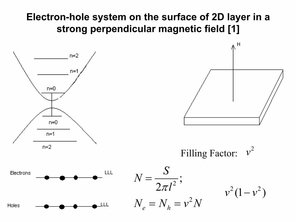
Electron-hole system on the surface of 2D layer in a strong perpendicular magnetic field [1]

2

2

;2

e h

SNl

N N v Nπ

=

= =

Filling Factor: 2v

2 2(1 )v v−

The action of the Lorentz force on the moving electron-hole pair [1]

The model of 2D magnetoexciton with wave vector k and dipole moment [1]

The most probable distances between the electron and hole inside the magnetoexciton [3]

,,

,( , , , ) ( , , , ) ( , )

( ) ( );

e h

e h

e h

e h

n nex e e h h ex n n

p q

ipx iqx

n e n h

x y x y x y C p q

e e y yL L

ψ ψ ξ η

φ φ

= = ×

×

∑

0; ; ; ; 2 2

1; ( )2

e h e he h e h e h

x

x x y yn n x x x y y y

k p q t p q

ξ η+ += = − = − = = =

= + = −

22 2 2 2

(0,0)2 2

2 2 2 22(0,0)2 2

( ) ( )( , ; , ) ;4 4

( ) ( )( , ; , ) exp4 4

yx ixikiky xl

ex

y xex

x k l y k le ex y e expl lL L

x k l y k lx yl l

ηηξ

ψ ξ η

ψ ξ η

− ⎡ ⎤− −= − −⎢ ⎥

⎢ ⎥⎣ ⎦⎡ ⎤− −− −⎢ ⎥⎢ ⎥⎣ ⎦

∼

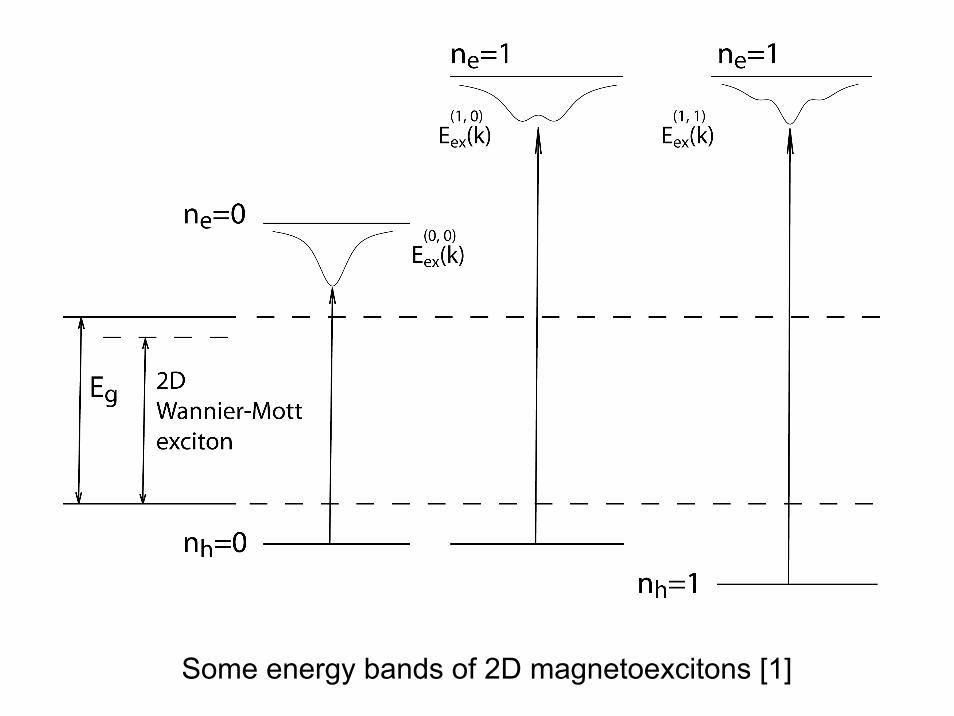
Some energy bands of 2D magnetoexcitons [1]

The dispersion laws for two 2D magnetoexciton energy bands [1]

The dispersion law and the group velocity of the lowest exciton energy band [1]

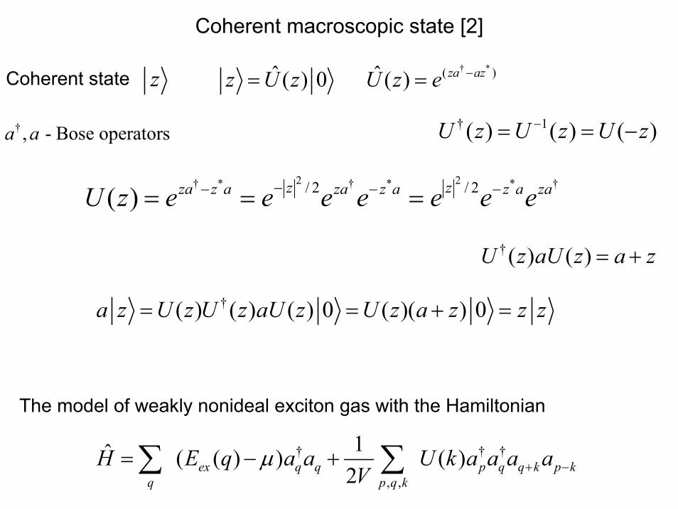
Coherent macroscopic state [2]

Coherent state z† *( )ˆ ˆ( ) 0 ( ) za azz U z U z e −= =

† 1( ) ( ) ( )U z U z U z−= = −† , - Bose operatorsa a

2 2† * † * * †/ 2 / 2( ) z zza z a za z a z a zaU z e e e e e e e−− − −= = =

† ( ) ( )U z aU z a z= +

†( ) ( ) ( ) 0 ( )( ) 0a z U z U z aU z U z a z z z= = + =

The model of weakly nonideal exciton gas with the Hamiltonian

† † †

, ,

1ˆ ( ( ) ) ( )2ex q q p q q k p k

q p q kH E q a a U k a a a a

Vμ + −= − +∑ ∑

The Bogoliubov canonical transformation introducing the coherent macroscopic state [2]

0 0 ,q k k q qa N δ α= +

00 0 0 0

0 0 0 0 0 0 0 0

†00 0 0

† † † † †0

ˆ ( ( ) ) [ ( ) ]( )2

[ ( ) ] ( ) ...2

kex k k k k

qex q q k q k q k q k q k q k q k q k q

q q

L NH E k N N E k L

LE q L

μ μ α α

μ α α α α α α α α α α+ + − − + − + −

= − + + + + +

+ + − + + + + +∑ ∑

00 0

2 2 2†4( ) ; (0) ; ( ) (0) ; ;

2k

k ex ex q q k k k k k k kex ex

N a qL U k U E q E T T u vV m mπ ξ α α+ −= = = + = = +

† 2[ ( ) ] ; ( ) 2 ;s k k k k kq

H U E k v k E k T T Lξ ξ= + + = +∑

0

**0( ) (0); ;

0k

sex ex

NE k u k k Uv um m Vk

== =

→

Keldysh-Kozlov-Kopaev method. Excitons as composite bosons [2]

2D magnetoexcitons in a strong perpendicular magnetic field [3]

† † † 2 † †1 1( ) ( ) ; ( ) 1; , - Fermi operatorsk q k q p pq q

d k q a b q a bVV α βϕ ϕ+ −= =∑ ∑

; ; e hex e h

ex ex

m m m m mm m

α β= = = +( ) †exp ( ( ) ( ))ex exD N N d k d k⎡ ⎤= −⎣ ⎦

2† † †2

2 2

1( ) ; ;2

y

x x

ik tlk kt tt

Sd k e a b NlN π

−

+ −= =∑

2 22 ; ; exex ex

N cg l n n lS eH

π= = =

( ) 2 2† †

2 2 2 2

exp y y

x x x x

ik tl ik tlex k k k kt t t tt

D N g e a b e a b−

+ − − +

⎡ ⎤⎛ ⎞= −⎢ ⎥⎜ ⎟

⎢ ⎥⎝ ⎠⎣ ⎦∏

Wave function of the new ground state [3]

( ) 2 † †

2 2

ˆ( ) 0 ; 0 0 0; ( ) 0y

x x

ik tlg ex p p g k kt tt

k D N a b k u ve a bψ ψ −

+ −

⎛ ⎞= = = = +⎜ ⎟

⎝ ⎠∏

22 2cos ; sin ; 1; ( ) yik tlu g v g u v v t ve−= = + = =

† † † †; ;2 2x xx x

p p p k p p p p k pk kDa D ua v p b Db D ub v p aα β− −

⎛ ⎞ ⎛ ⎞= = − − = = + −⎜ ⎟ ⎜ ⎟⎝ ⎠ ⎝ ⎠

† †; 2 2x xx x

p p k p p p k pk ka u v p b u v pα β β α− −

⎛ ⎞ ⎛ ⎞= + − = − −⎜ ⎟ ⎜ ⎟⎝ ⎠ ⎝ ⎠

† †( ) 0 0 0; ( ) 0 0 0;p g p p p g p pk Da D D Da k Db D D Dbα ψ β ψ= = = = = =

† 2 2 2 2 2( ) ( ) ; 2 sin ;exex g p p g ex

p

NN k a a k Nv n l g v gN

ψ ψ π= = = = = =∑ 2 1v

22 2

2 2

1 sin ; 1; ;2 2exvg g g nl lπ π

= =

Breaking of the gauge symmetry [3]

Compensation of the dangerous diagrams

†2

2 † † 2 † †2

;

( , , )( ) ( , , ) 2 2x xx x

p p p p k p p p k pp p

H DHD U H H

k kH E k v u k v v p v pμ α α β β ψ μ β α α β− −

′= = + +

⎡ ⎤⎛ ⎞ ⎛ ⎞= + − − + −⎜ ⎟ ⎜ ⎟⎢ ⎥⎝ ⎠ ⎝ ⎠⎣ ⎦∑ ∑

( ) ( )( )

2 2 2 4 2 2 2 2

2 2 2 2

( , , ) 2 ( ) ; 2

( , , ) 2 ( )

ex l

l ex

E k v u v I k I v u v u v

k v v I I k u v

μμ

ψ μ μ

= + − − −

= + − +

2 2 2 2 24

00

( ) ; 4 2

k l

ex l lk l eI k I e I I

lπ

ε− ⎛ ⎞

= =⎜ ⎟⎝ ⎠

( )

2

2

( , , ) 0;( ) 2 ( ) ; ( ) ( )HFB

ex l ex ex ex

k vE k v I I k E k I k

ψ μ

μ

=

= − − = −

( ) ( ) ( ) ( )0 0 int 0ˆ ˆE T Hλ λ λ λ= Ψ + Ψ

( ) ( )intˆ ˆ ˆ ;H T Hλ λ= + ( ) ( ) ( ) ( )0 0 0H Eλ λ λ λΨ = Ψ

( ) ( ) ( ) ( )int 0 int 0ˆ ;E Hλ λ λ λ= Ψ Ψ ( )intH λ λ≈

( ) ( )0 0 1λ λΨ Ψ =

( ) ( ) ( ) ( ) ( ) ( )0 int int0 0 0

E E EE

λ λ λλ λ λ

λ λ λ λ∂ ∂

= + Ψ Ψ =∂ ∂

( ) ( ) ( ) ( )2 2

0 20 0 int

0 0

0e eE dd E e E E

λ λλ λ λλ λ

∂= − = =

∂∫ ∫

( )2

0 int0

e

kindE E Eλ λλ

= + ∫

Pauli-Feynman’s theorem [2]

( ) ( ) †int

1ˆ ˆ ˆˆ ˆ2 e hk k k

k

H V N Nλ λ ρ ρ⎡ ⎤= − −⎣ ⎦∑

† †ˆ p pk p k p kk k

a a b bρ+ +

= −∑ ∑

†ˆ ;e p pp

N a a=∑†ˆ

h p pp

N b b=∑

( ) ( ) ( ) ( )2

†int ,0

( )

12ex k k k n

nk k

E N V Vλ

λ λ λ ρ= − +∑ ∑ ∑

( ) ( )2

†

,0( ) 0

1 12 2 ( , , )k k n

n

dV mkλ

ωλ ρπ ε ω λ

∞ ⎛ ⎞= − ℑ ⎜ ⎟

⎝ ⎠∑ ∫

( )2

†

,0,0 ,0

1 1 1( , )

kk n

n n n

Vi ik

ρω ω δ ω ω δε ω

⎡ ⎤= −⎢ ⎥

− + + +⎢ ⎥⎣ ⎦∑

The BCS-type ground state wave function of the BEC 2D magnetoexcitons and their Anderson-type coherent excited states [3]

( )( )

( )( ) ( )

1 21 23 5

2 2 2

23 5 3 3

3;

31 3

2

non cond

cond

d R d Rd dVR R

dR Rdd d dV Cos

R R R Rθ

⎡ ⎤⎢ ⎥−⎢ ⎥⎣ ⎦

⎡ ⎤⎢ ⎥− ≈ − = −⎢ ⎥⎢ ⎥⎣ ⎦

∼

∼

2 † †

2 2

( ) 0y

x x

k tlg k kt tt

k u ve a bψ −

+ −

⎛ ⎞= +⎜ ⎟

⎝ ⎠∏ †

2 2

( )2 x x

e xQ Q gq q

Qq a a kψ ψ+ −

⎛ ⎞± =⎜ ⎟⎝ ⎠

Polarizability of the Bose-Einstein condensed magnetoexcitons.Anderson-type wave functions of the coherent excited states [3]

2 2 ( , ) ( , )2 2

e ex xkr x x kr

P Qp q u v P Q p qψ ψ δ δ⎛ ⎞ ⎛ ⎞± ± =⎜ ⎟ ⎜ ⎟⎝ ⎠ ⎝ ⎠

†

2 2

( ) ;2 x x

e xQ Q gq q

Qq a a kψ ψ+ −

⎛ ⎞± =⎜ ⎟⎝ ⎠

22 2 ( );2

2 2

e ex x

xex

e ex x

P Pp H pPE p I k

P Pp p

ψ ψ

ψ ψ

⎛ ⎞ ⎛ ⎞± ±⎜ ⎟ ⎜ ⎟⎛ ⎞ ⎝ ⎠ ⎝ ⎠± = =⎜ ⎟ ⎛ ⎞ ⎛ ⎞⎝ ⎠ ± ±⎜ ⎟ ⎜ ⎟⎝ ⎠ ⎝ ⎠

( )22

† 2 2 200

[ ]( , )4 sin ; ( )2

zQ kr x x n exn

K Q lP Q u v I kρ δ ω⎛ ⎞×

= =⎜ ⎟⎝ ⎠

1 ; 0 ( )2

e xg

Pn p kuv

ψ ψ⎛ ⎞= ± =⎜ ⎟⎝ ⎠

Polarizability 04 ( , )HF Qπα ω

( ) ( )2 2

†

0 00

,0 ,0

22 2 2

4 ( , )

[ ] 1 14 sin2 ( ) ( )

Q QQ n nHF

n n n

zQ

ex ex

WQ

i i

K Q lu v W NI k i I k i

ρ ρπα ω

ω ω δ ω ω δ

ω δ ω δ

⎡ ⎤⎢ ⎥= − − =⎢ ⎥− + + +⎢ ⎥⎣ ⎦⎡ ⎤⎛ ⎞×

= − −⎜ ⎟ ⎢ ⎥− + + +⎝ ⎠ ⎣ ⎦

∑

2 222

00

1; 1 4 ( , )( , )

Q lHF

Q HF

eW e QQS Q

πα ωε ωε

−= − = −

2, ( , ) [ ( , ) ] ...

1 ( , ) ( , )Q Q

Q eff Q Q Q Q Q RPAQ

W WW W W Q W W Q W

Q W Qπ ω π ω

π ω ε ω= + + + = =

−

0( , ) 1 4 ( , );RPA HFQ Qε ω πα ω= +

1 2( , , ) ( , , ) ( , , )Q Q i Qε ω λ ε ω λ ε ω λ= +

[3]

Screening effects and correlation energy [3]

2

2210

( , , )1Im( , , ) ( , , )

e QdQ Q

ε ω λλλ ε ω λ ε ω λ

≈ −∫

0,2 0,10

2 4 ( , )4 ( , )2

HF HFcorr

Q

dE Q Qω πα ω πα ωπ

∞

= − ∑ ∫

( )

2 22 2

22 2 2 2

2 2 2 282

0 0

2 ( )2 ( ) (1 )(1 2 )( )

( ) 3 42 8

HFB lcorr ex l ex

ex

k lk l

I F klI v I I k v v vI k

k l k lF kl e I e I

μ μ μπ

−−

= + = − − − − − −

⎛ ⎞ ⎛ ⎞= + −⎜ ⎟ ⎜ ⎟

⎝ ⎠ ⎝ ⎠

Chemical potential versus filling factor v2. Solid line: total chemical potential. Dashing line: chemical potential in HFBA at

kl=4,6 [3]

a)

b)

Chemical potential versus filling factor v2. [3]

a) The same as on the previous slide.b) The taking into account of the magnetoexciton damping rate.

2

2

2

2

†

2 2

†

2 2

† † †

2 2

2 2

ˆ ( ) ;

ˆ ( ) ;

ˆ ˆ ˆ( ) ( ) ( );ˆ ˆ ˆ( ) ( ) ( );

1( ) ;

1( ) ;

y

x x

y

x x

y

x x

y

x x

iQ tle Q Qt tt

iQ tlh Q Qt tt

e h

e h

iP tlP Pt tt

iP tlP Pt tt

Q e a a

Q e b b

Q Q Q

D Q Q Q

d P e a bN

d P e b aN

ρ

ρ

ρ ρ ρ

ρ ρ

− +

+ −

−

+ − +

− + +

=

=

= − −

= + −

=

=

∑

∑

∑

∑

ˆ ˆ (0);ˆ ˆ (0);

ˆ ˆˆ (0) ;ˆ ˆ ˆ(0) ;

e e

h h

e h

e h

N

N

N N

D N N

ρ

ρ

ρ

=

=

= −

= +

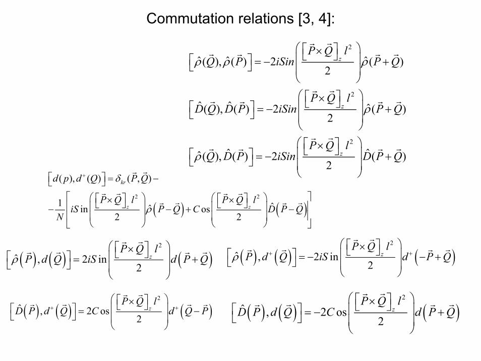
Two-particle operators describing the density fluctuations as well as the creation and annihilation of 2D magnetoexcitons [3], [4]

Collective elementary excitations

2

2

2

ˆ ˆ ˆ( ), ( ) 2 ( )2

ˆ ˆ ˆ( ), ( ) 2 ( )2

ˆ ˆˆ ( ), ( ) 2 ( )2

z

z

z

P Q lQ P iSin P Q

P Q lD Q D P iSin P Q

P Q lQ D P iSin D P Q

ρ ρ ρ

ρ

ρ

⎛ ⎞⎡ ⎤×⎣ ⎦⎜ ⎟⎡ ⎤ = − +⎣ ⎦ ⎜ ⎟⎝ ⎠⎛ ⎞⎡ ⎤×⎣ ⎦⎜ ⎟⎡ ⎤ = − +⎣ ⎦ ⎜ ⎟⎝ ⎠⎛ ⎞⎡ ⎤×⎣ ⎦⎜ ⎟⎡ ⎤ = − +⎣ ⎦ ⎜ ⎟⎝ ⎠

( ) ( )2 2

( ), ( ) ( , )

1 ˆˆin os2 2

kr

z z

d p d Q P Q

P Q l P Q liS P Q C D P Q

N

δ

ρ

+⎡ ⎤ = −⎣ ⎦⎡ ⎤⎛ ⎞ ⎛ ⎞⎡ ⎤ ⎡ ⎤× ×⎣ ⎦ ⎣ ⎦⎢ ⎥⎜ ⎟ ⎜ ⎟− − + −⎢ ⎥⎜ ⎟ ⎜ ⎟

⎝ ⎠ ⎝ ⎠⎣ ⎦

( ) ( ) ( )2

ˆ , 2 in2

zP Q l

P d Q iS d P Qρ⎛ ⎞⎡ ⎤×⎣ ⎦⎜ ⎟⎡ ⎤ = +⎣ ⎦ ⎜ ⎟⎝ ⎠

( ) ( ) ( )2

ˆ , 2 in2

zP Q l

P d Q iS d P Qρ + +⎛ ⎞⎡ ⎤×⎣ ⎦⎜ ⎟⎡ ⎤ = − − +⎣ ⎦ ⎜ ⎟⎝ ⎠

( ) ( ) ( )2

ˆ , 2 os2

zP Q l

D P d Q C d Q P+ +⎛ ⎞⎡ ⎤×⎣ ⎦⎜ ⎟⎡ ⎤ = −⎣ ⎦ ⎜ ⎟⎝ ⎠

( ) ( ) ( )2

ˆ , 2 os2

zP Q l

D P d Q C d P Q⎛ ⎞⎡ ⎤×⎣ ⎦⎜ ⎟⎡ ⎤ = − +⎣ ⎦ ⎜ ⎟⎝ ⎠

Commutation relations [3, 4]:

1ˆ ˆ ˆ ˆ ˆˆ ˆ( ) ( )2 e h e e h hQ

Q

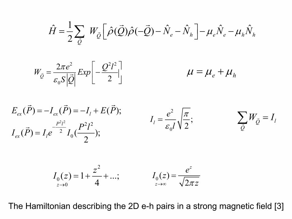
H W Q Q N N N Nρ ρ μ μ⎡ ⎤= − − − − −⎣ ⎦∑

2 2 2

0

22Q

e Q lW ExpS Qπ

ε⎡ ⎤

= −⎢ ⎥⎣ ⎦

e hμ μ μ= +

2 2 2 22

0

( ) ( ) ( );

( ) ( );2

ex ex l

P l

ex l

E P I P I E P

P lI P I e I−

= − = − +

=

2

0

;2l

eIl

πε

= lQQ

W I=∑

2

00

( ) 1 ...;4z

zI z→

= + + 0 ( )2

z

z

eI zzπ→∞

=

The Hamiltonian describing the 2D e-h pairs in a strong magnetic field [3]

( ) ( )†

1ˆ ˆ ˆ ˆ ˆ( ) ( )2

( ) ( ) ( ) ;

e h e e h hQQ

i il

W Q Q N N N N

N e d k e d k E k v Iϕ ϕ

ρ ρ μ μ

η η μ μ μ−

⎡ ⎤= − − − − − −⎣ ⎦

− + = − = +

∑H

2

2 2

ˆ( ) [ ( ), ] ( ( ) ) ( ) ( , )

[ ] ˆ2 ( ) ( )2

ˆˆ[ ] [ ]( ) ( ) ;2 2

ikr

zQ

Q

i z z

di d P d P E P d P Ne P Kdt

P Q li W Sin Q d P Q

P K l P K lP K D P Ke iSin CosN N

ϕ

ϕ

μ η δ

ρ

ρη

= = − − −

⎛ ⎞×− − +⎜ ⎟

⎝ ⎠⎡ ⎤⎛ ⎞ ⎛ ⎞× ×− −

+ +⎢ ⎥⎜ ⎟ ⎜ ⎟⎢ ⎥⎝ ⎠ ⎝ ⎠⎣ ⎦

∑

H

Equations of motion:

The breaking of the gauge symmetry as in the Bogoliubov’stheory of quasi-averages [4].

† † †

2†

2 2

ˆ(2 ) [ (2 ), ] ( (2 )) (2 )

[(2 ) ] ˆ( , ) 2 (2 ) ( )2

ˆˆ[ ] [ ]( ) ( )2 2

i zkr Q

Q

i z z

di d K P d K P E K P d K Pdt

K P Q lNe P K i W Sin d K P Q Q

P K l P K lP K D P Ke iSin CosN N

ϕ

ϕ

μ

η δ ρ

ρη

−

−

− = − = − − − +

⎛ ⎞− ×+ − − − − −⎜ ⎟

⎝ ⎠⎡ ⎛ ⎞ ⎛ ⎞× ×− −

− +⎢ ⎜ ⎟ ⎜ ⎟⎝ ⎠ ⎝ ⎠⎣

∑

H

⎤⎥

⎢ ⎥⎦

Equations of motion:

2

2†

ˆˆ ˆ( ) ( ),

[( ) ] ˆ ˆ ˆ ˆ[ ( ) ( ) ( ) ( )]2

[ ]2 ( ) (2 ) ;2

ˆˆ ˆ( ) [ ( ), ]

zQ

Q

i iz

QQ

di P K P Kdt

P K Q li W Sin P K Q Q Q P K Q

P K li NSin e d P e d K P

di D P K D P Kdt

i W Sin

ϕ ϕ

ρ ρ

ρ ρ ρ ρ

η −

⎡ ⎤− = − =⎣ ⎦

⎛ ⎞− ×= − − − + − − −⎜ ⎟

⎝ ⎠⎛ ⎞× ⎡ ⎤− − −⎜ ⎟ ⎣ ⎦⎝ ⎠

− = − =

−

∑

∑

H

H

2

2†

[( ) ] ˆ ˆˆ ˆ[ ( ) ( ) ( ) ( )]2

[ ]2 ( ) (2 ) ;2

z

i iz

P K Q l Q D P K Q D P K Q Q

P K lNCos e d P e d K Pϕ ϕ

ρ ρ

η −

⎛ ⎞− ×− − + − − +⎜ ⎟

⎝ ⎠⎛ ⎞× ⎡ ⎤+ − −⎜ ⎟ ⎣ ⎦⎝ ⎠

2

2

2

[ ] ˆ ˆ ˆ ˆ[ ( ) ( ) ( ) ( )]2

[ ]ˆ ˆ ˆ( ) ( ) 2 ( ) ( )2

[ ]ˆ ˆ ˆ( ) ( ) 2 ( ) ( ) ...2

zQ

Q

zQ

Q

zQ

Q

P Q li W Sin Q P Q P Q Q

P Q lE P P i W Sin Q P Q

P Q lE P P i W Sin P Q Q

ρ ρ ρ ρ

ρ ρ ρ

ρ ρ ρ

⎛ ⎞×− − + − =⎜ ⎟

⎝ ⎠⎛ ⎞×

= − − =⎜ ⎟⎝ ⎠⎛ ⎞×

= − − − =⎜ ⎟⎝ ⎠

∑

∑

∑

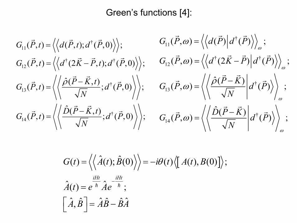
†11

† †12

†13

†14

( , ) ( , ); ( ,0) ;

( , ) (2 , ); ( ,0) ;

ˆ ( , )( , ) ; ( ,0) ;

ˆ ( , )( , ) ; ( ,0) ;

G P t d P t d P

G P t d K P t d P

P K tG P t d PN

D P K tG P t d PN

ρ

=

= −

−=

−=

[ ]ˆ ˆ( ) ( ); (0) ( ) ( ), (0) ;

ˆ ˆ( ) ;ˆ ˆ ˆˆ ˆ ˆ,

iHt iHt

G t A t B i t A t B

A t e Ae

A B AB BA

θ

−

= = −

=

⎡ ⎤ = −⎣ ⎦

†11

† †12

†13

†14

( , ) ( ) ( ) ;

( , ) (2 ) ( ) ;

ˆ ( )( , ) ( ) ;

ˆ ( )( , ) ( ) ;

G P d P d P

G P d K P d P

P KG P d PN

D P KG P d PN

ω

ω

ω

ω

ω

ω

ρω

ω

=

= −

−=

−=

Green’s functions [4]:

11

2†

2 2

13 14

12

[ ( ) ] ( , )

[ ] ˆ2 ( ) ( ) ( )2

[ ] [ ]( , ) ( , ) ;2 2

[ (2 ) ] ( , )

[(22

zQ

Q

i z z

QQ

E P i G P C

P Q li W Sin Q d P Q d P

P K l P K le iSin G P Cos G P

E K P i G P C

Ki W Sin

ω

ϕ

ω μ δ ω

ρ

η ω ω

ω μ δ ω

+ − + = −

⎛ ⎞×− − +⎜ ⎟

⎝ ⎠⎡ ⎤⎛ ⎞ ⎛ ⎞× ×

+ +⎢ ⎥⎜ ⎟ ⎜ ⎟⎢ ⎥⎝ ⎠ ⎝ ⎠⎣ ⎦

− + − + = −

−

∑

∑2

† †

2 2

13 14

) ] ˆ(2 ) ( ) ( )2

[ ] [ ]( , ) ( , ) ;2 2

z

i z z

P Q l d K P Q Q d P

P K l P K le iSin G P Cos G P

ω

ϕ

ρ

η ω ω−

⎛ ⎞− ×− − − −⎜ ⎟

⎝ ⎠⎡ ⎤⎛ ⎞ ⎛ ⎞× ×

− +⎢ ⎥⎜ ⎟ ⎜ ⎟⎢ ⎥⎝ ⎠ ⎝ ⎠⎣ ⎦13

2†

2

11 12

14

[ ] ( , )

ˆ ˆ[( ) ] ( ) ( )ˆ ˆ( ) ( ) ( )2

[ ]2 ( , ) ( , ) ;2

[ ] ( , )

[( )

zQ

Q

i iz

QQ

i G P C

P K Q l P K Q P K Qi W Sin Q Q d PN N

P K li Sin e G P e G P

i G P C

P Ki W Sin

ω

ϕ ϕ

ω δ ω

ρ ρρ ρ

η ω ω

ω δ ω

−

+ = −

⎛ ⎞ ⎡ ⎤− × − − − −− + −⎜ ⎟ ⎢ ⎥

⎣ ⎦⎝ ⎠

⎛ ⎞× ⎡ ⎤− −⎜ ⎟ ⎣ ⎦⎝ ⎠

+ = −

− ×−

∑

∑2

†

2

11 12

ˆ ˆ] ( ) ( )ˆ ˆ( ) ( ) ( )2

[ ]2 ( , ) ( , ) ;2

z

i iz

Q l D P K Q D P K QQ Q d PN N

P K lCos e G P e G P

ω

ϕ ϕ

ρ ρ

η ω ω−

⎡ ⎤⎛ ⎞ − − − −+ +⎜ ⎟ ⎢ ⎥

⎝ ⎠ ⎣ ⎦

⎛ ⎞× ⎡ ⎤+ −⎜ ⎟ ⎣ ⎦⎝ ⎠

Equations of motion for Green’s functions [4]:

22 2

11

22

22 2

21

31

ˆ ˆ( ) ( )[ ]( , ) ( ( ) ) 42 ( )

[ ]4 v( )2

;( )

[ ]4 v( )2

( , ) ;( )

(

zQ

Q

zP K

i zP K

Q QP Q lP E P i W SinE P Q i

P K lW N Sin

E K i

P K le W N SinP

E K i

P

ϕ

ρ ρω ω μ δ

ω μ δ

η

ω μ δ

ηω

ω μ δ

−

−

−⎛ ⎞×Σ = + − + − −⎜ ⎟

+ − − +⎝ ⎠⎛ ⎞×⎜ ⎟⎝ ⎠−

+ − +

⎛ ⎞×⎜ ⎟⎝ ⎠Σ =

+ − +

Σ

∑

2

2

2

2

2( )[ ], ) 12 ( )

[ ]42 [ ] ˆ( ) ( )

2( )

[( ) ( )][ ]4

2

i z P K

zP K

zR

R

z

zP KQ

Q

W NP K li e SinE K i

P K lW SinR K lW Sin R d K R N

E K i

P Q P KSinP Q lW W Sin

ϕω ηω μ δ

ρω μ δ

−

−

−

⎛ ⎞⎛ ⎞×= − − +⎜ ⎟⎜ ⎟+ − +⎝ ⎠⎝ ⎠⎛ ⎞×⎜ ⎟ ⎛ ⎞×⎝ ⎠+ − +⎜ ⎟+ − + ⎝ ⎠

− × −⎛ ⎞×

+ ⎜ ⎟⎝ ⎠

∑

∑

2

2 2

2

41

ˆ ( ) ( )2

( )

ˆ ( ) ( )[ ] [( ) )]4 ( ) ;2 2 ( )

[ ]( , ) ;2

z zP KQ Q K P

Q

i z

l Q d K Q N

E P Q i

Q K P d P Q NP Q l P K Q lW W W Sin SinE P Q i

P K lP e Cosϕ

ρ

ω μ δ

ρ

ω μ δ

ω η

−+ −

⎛ ⎞−⎜ ⎟

⎝ ⎠ ++ − − +

+ − −⎛ ⎞ ⎛ ⎞× − ×+ − ⎜ ⎟ ⎜ ⎟

+ − − +⎝ ⎠ ⎝ ⎠⎛ ⎞×

Σ = − ⎜ ⎟⎝ ⎠

∑

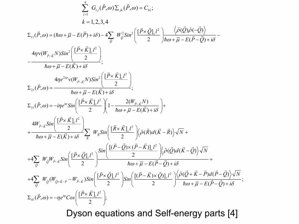
4

1 11

( , ) ( , ) ;

1, 2,3, 4

j jk kj

G P P C

k

ω ω=

∑ =

=

∑

Dyson equations and Self-energy parts [4]

22 2

12

22

222

22

[ ]v( )2

( , ) 4 ;( )

[(2 ) ] ˆ ˆ( ) ( )2

( , ) (2 ) 4(2 )

[ ]( )2

4 v(

i zK P

z

QQ

zP K

P K le W N SinP

E K i

K P Q lSin Q QP E K P i W

E K P Q i

P K lW N Sin

E

ϕ

ω ηω μ δ

ρ ρω ω μ δ

ω μ δ

ηω μ

−−

−

⎛ ⎞×⎜ ⎟⎝ ⎠Σ =

− + +

⎛ ⎞− ×−⎜ ⎟

⎝ ⎠Σ = − + − + − −− + − − +

⎛ ⎞×⎜ ⎟⎝ ⎠−

− +

∑

;)K iδ+

2

32

2

2†

2

2( )[ ]( , ) 12 ( )

[ ]2 [ ] ˆ4 ( ) ( )

2( )

[(2 ) ] [(242

i z P K

zP K

zR

R

zK PQ

Q

W NP K lP i e SinE K i

P K lW SinR K lW Sin d K R R N

E K i

K P Q lW W Sin Sin

ϕω ηω μ δ

ρω μ δ

− −

−

−

⎛ ⎞ ⎡ ⎤×Σ = + −⎜ ⎟ ⎢ ⎥− + +⎣ ⎦⎝ ⎠

⎛ ⎞×⎜ ⎟ ⎛ ⎞×⎝ ⎠− − − +⎜ ⎟− + + ⎝ ⎠

⎛ ⎞− ×+ ⎜ ⎟

⎝ ⎠

∑

∑†2

†2 2

42

ˆ( ) ( )) ( )]2 (2 )

ˆ(2 ) ( )[(2 ) ] [( ) ]4 ( ) ;2 2 (2 )

( , )

z

z zP KQ P K Q

Q

d K Q Q NK P Q K P lE K P Q i

d K P Q K P Q NK P Q l P K Q lW W W Sin SinE K P Q i

P

ρ

ω μ δ

ρ

ω μ δ

ω η

− − +

− −⎛ ⎞− − × −+⎜ ⎟

− + − − +⎝ ⎠

− − − −⎛ ⎞ ⎛ ⎞− × − ×+ − ⎜ ⎟ ⎜ ⎟

− + − − +⎝ ⎠ ⎝ ⎠

Σ =

∑2[ ] ;

2i zP K le Cosϕ− ⎛ ⎞×

⎜ ⎟⎝ ⎠

Self-energy parts

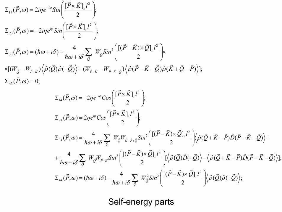
2

13

2

23

22

33

[ ]( , ) 2 ;2

[ ]( , ) 2 ;2

[( ) ]4( , ) ( )2

ˆ ˆ ˆ ˆ[( ) ( ) ( ) ( ) ( ) (

i z

i z

zQ

Q

P K P KQ P K Q

P K lP i e Sin

P K lP i e Sin

P K Q lP i W Sini

W W Q Q W W P K Q K Q

ϕ

ϕ

ω η

ω η

ω ω δω δ

ρ ρ ρ ρ

−

− − − −

⎛ ⎞×Σ = ⎜ ⎟

⎝ ⎠⎛ ⎞×

Σ = − ⎜ ⎟⎝ ⎠

⎛ ⎞− ×Σ = + − ×⎜ ⎟+ ⎝ ⎠

× − − + − − − + −

∑

43

) ];

( , ) 0;

P

P ωΣ =

2

14

2

24

22

34

22

[ ]( , ) 2 ;2

[ ]( , ) 2 ;2

[( ) ]4 ˆˆ( , ) ( ) ( )2

[( ) ]42

i z

i z

zQ K P Q

Q

zP KQ

Q

P K lP e Cos

P K lP e Cos

P K Q lP W W Sin Q K P D P K Qi

P K Q lW W Sini

ϕ

ϕ

ω η

ω η

ω ρω δ

ω δ

−

− +

−

⎛ ⎞×Σ = − ⎜ ⎟

⎝ ⎠⎛ ⎞×

Σ = ⎜ ⎟⎝ ⎠

⎛ ⎞− ×Σ = + − − − +⎜ ⎟+ ⎝ ⎠

⎛ ⎞− ×+ ⎜+ ⎝ ⎠

∑

∑2

2 244

ˆ ˆˆ ˆ[ ( ) ( ) ( ) ( ) ];

[( ) ]4 ˆ ˆ( , ) ( ) ( ) ( ) ;2

zQ

Q

Q D Q Q K P D P K Q

P K Q lP i W Sin Q Qi

ρ ρ

ω ω δ ρ ρω δ

− − + − − −⎟

⎛ ⎞− ×Σ = + − −⎜ ⎟+ ⎝ ⎠

∑

Self-energy parts

22 2 2 [ ]ˆ ˆ( ) ( ) 4 v

2zK Q lQ Q u NSinρ ρ

⎛ ⎞×− = ⎜ ⎟

⎝ ⎠

33( ; ) 0;K q ωΣ + = [ ] 0zq K× =

211 22 44 11 22( , ) ( , ) ( , ) 2 ( ( , ) ( , )) 0K q K q K q K q K qω ω ω η ω ωΣ + Σ + Σ + − Σ + +Σ + =

det ( , ) 0;ij P P K qω∑ = = +

Dispersion equations in collinear geometry [4]

The dispersion equations in the collinear geometry [4]

33( , ) 0 ; 0 ;z

k q q kω ⎡ ⎤Σ + = × =⎣ ⎦

( )

( )

211 22 44 11 22

211 22 44 11 22

( , ) ( , ) ( , ) 2 ( , ) ( , ) 0

( , ) ( , ) ( , )

( , ) ( , ) ( , ) 2 ( , ) ( , ) 0

ij ij ij

k q k q k q k q k q

k q k q i k q

k q k q k q k q k q

ω ω ω η ω ω

ω σ ω ω

σ ω σ ω σ ω η σ ω σ ω

Σ + Σ + Σ + − Σ + +Σ + =

Σ + = + + Γ +

+ + + − + + + =

; ; 0 ; 1P k q P k q Cos q Cosα α= + = + ⋅ > = ±

( )

11 22( ) ( ) ( )

( )

2 ( ) ( )g

k q k q E k q

E k q

V k q

σ σ ω μ

ω μ

ω+ −

+ −

+ + + = + − + +

+ − + − − − =

= − ⋅ − +

L L

L L

( )

( )

2

11 22

22 2

2 2

( ) ( ) ( )

( ) ( ) ( )2 ( )

( ) ( )2 ( )

g

g

k q k q V k q

qE k V k qM k

qE kM k

σ σ ω

μ ω

μ

+ −

+ − + −

+ ⋅ + = − ⋅ −

⎛ ⎞− − − − + − ⋅ +⎜ ⎟⎝ ⎠

⎛ ⎞+ − − − +⎜ ⎟

⎝ ⎠

L L

L L L L

( )

2

2 22 2

ˆ ˆ( ) ( ) ( )4

2( ) ( )

2 ( )3 4; 1

zQ

Qg

k q Q l Q QW Sin

qV k Q q E k QM k Q

kl Ql

ρ ρ

ω μ±

⎛ ⎞⎡ ⎤± × −⎣ ⎦⎜ ⎟=⎜ ⎟ ⎛ ⎞⎝ ⎠ − − ⋅ ± − − −⎜ ⎟−⎝ ⎠

− ≈

∑

∼

L

Dispersion law for free magnetoexciton [4]

2

00

v 0

00

g

kv

μη===

=

=

Energy spectrum of the ideal magnetoexciton gas moving as a whole as regards the laboratory reference frame with the group velocity

6

2

0.2360

v 1.68*10 / sec

3,60

l

g

I

cm

klv

μη= −=

=

=

=

v ( )g k [4]

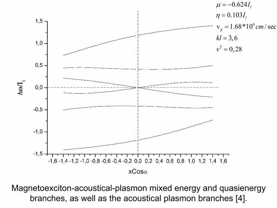
Magnetoexciton-acoustical-plasmon mixed energy and quasienergybranches, as well as the acoustical plasmon branches [4].

6

2

0.2790.000103

v 1.68*10 / sec

3,60,03

l

l

g

II

cm

klv

μη= −=

=

=

=

6

2

0.6240.103

v 1.68*10 / sec

3,60,28

l

l

g

II

cm

klv

μη= −=

=

=

=

Magnetoexciton-acoustical-plasmon mixed energy and quasienergybranches, as well as the acoustical plasmon branches [4].

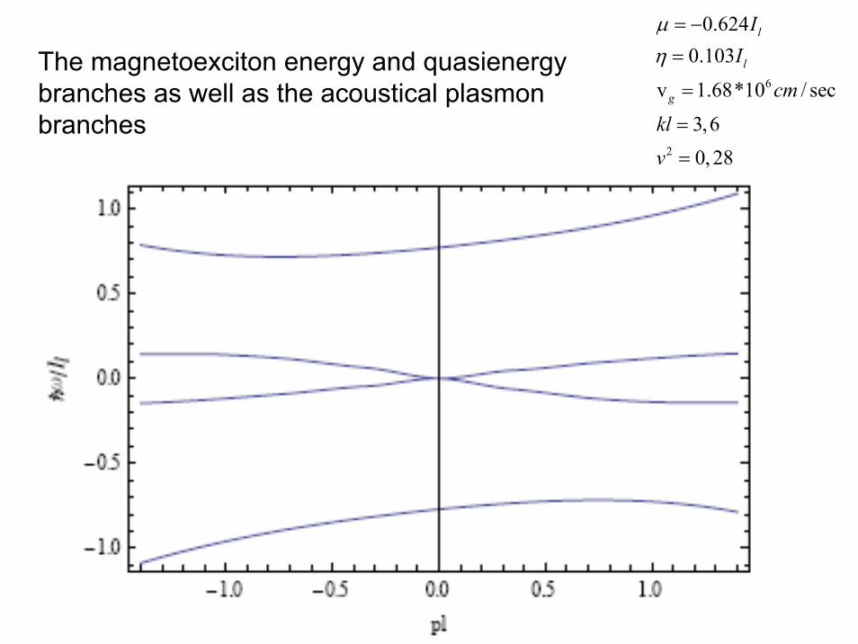
The magnetoexciton energy and quasienergybranches as well as the acoustical plasmon branches

6

2

0.6240.103

v 1.68*10 / sec

3,60,28

l

l

g

II

cm

klv

μη= −

=

=

=

=

Part 2

Collective elementary excitations oftwo-dimensional magnetoexcitons in a

state of Bose-Einstein condensation with wave vector kl=0 [5, 6]

Starting Hamiltonian [5]

Here the zero order Hamiltonian is:

0ˆ ˆ ˆ ˆLLL ELL

Coul CoulH H H H= + +

† †0

1 1

ˆce np np ch np np

n p n p

H n c c n d dω ω∞ ∞

= =

= +∑∑ ∑∑

The Coulomb interaction in the frame of the LLLs has the form [5]:

† †

, ,

† †

, ,

† †

, ,

1ˆ ( ,0; ,0; ,0; ,0)2

1 ( ,0; ,0; ,0; ,0)2

( ,0; ,0; ,0; ,0)

LLLCoul e e p q q s p s

p q s

h h p q q s p sp q s

e h p q q s p sp q s

H F p q p s q s a a a a

F p q p s q s b b b b

F p q p s q s a b b a

− + −

− + −

− + −

= − + +

+ − + −

− − +

∑

∑

∑

and the virtual quantum transitions are [5]: (0,0) ( , )n m

† †

, , ,

† †, ,

, , ,

† †

, , ,

,

1 ( , ; , ; ,0; ,0)2

1 ( ,0; ,0; , ; , )21 ( , ; , ; ,0; ,0)21 ( ,0; ,0; ,2

ELLCoul e e np mq q s p s

p q s n m

e e p q m q s n p sp q s n m

h h np mq q s p sp q s n m

h hn m

H F p n q m p s q s c c a a

F p q p s n q s m a a c c

F p n q m p s q s d d b b

F p q p s n

− + −

− + −

− + −

−

= − + +

+ − + +

+ − + +

+ −

∑∑

∑∑

∑∑

∑ † †, ,

, ,

† †

, , ,

† †, ,

, , ,

; , )

( , ; , ; ,0; ,0)

( ,0; ,0; , ; , )

p q m q s n p sp q s

e h np mq q s p sp q s n m

e h p q m q s n p sp q s n m

q s m b b d d

F p n q m p s q s c d b a

F p q p s n q s m a b d c

+ −

− + −

− + −

+ −

− − + −

− − +

∑

∑∑

∑∑

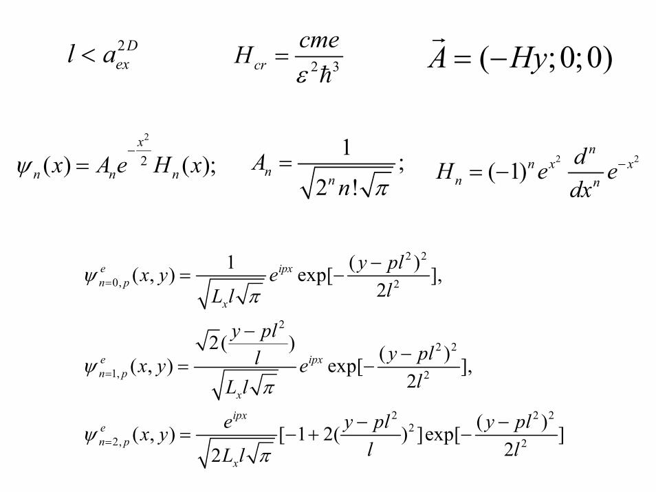
( ;0;0)A Hy= −2Dexl a< 2 3cr

cmeHε

=

2 2

0, 2

2

2 2

1, 2

2 2 22

2, 2

1 ( )( , ) exp[ ],2

2( ) ( )( , ) exp[ ],2

( )( , ) [ 1 2( ) ]exp[ ]22

e ipxn p

x

e ipxn p

x

ipxen p

x

y plx y elL l

y ply pllx y elL l

e y pl y plx yl lL l

ψπ

ψπ

ψπ

=

=

=

−= −

−−

= −

− −= − + −

2

2( ) ( );x

n n nx A e H xψ−

=1 ;

2 !n nA

n π= 2 2

( 1)n

n x xn n

dH e edx

−= −

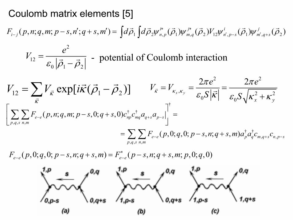
Coulomb matrix elements [5]

1 2 , 1 , 2 12 , 1 , 2( , ; , ; , ; , ) ( ) ( ) ( ) ( )i j i ji j n p m q n p s m q sF p n q m p s n q s m d d Vρ ρ ψ ρ ψ ρ ψ ρ ψ ρ∗ ∗

′ ′− − +′ ′− + = ∫ ∫2

120 1 2

eVε ρ ρ

=− - potential of Coulomb interaction

12 1 2exp[ ( )]V V iκκ

κ ρ ρ= −∑2 2

, 2 20 0

2 2x y

x y

e eV VS S

κ κ κπ π

ε κ ε κ κ= = =

+†

† †

, , ,

† †, ,

, , ,

( , ; , ; ,0; ,0)

( ,0; ,0; , ; , )

e e np mq q s p sp q s n m

e e p q m q s n p sp q s n m

F p n q m p s q s c c a a

F p q p s n q s m a a c c

− + −

− + −

⎡ ⎤− + =⎢ ⎥

⎣ ⎦= − +

∑∑

∑∑

( ,0; ,0; , ; , ) ( , ; , ; ,0; ,0)e e e eF p q p s n q s m F p s n q s m p q∗− −− + = − +

The coefficients describing the electron–hole Coulomb interaction involving the simultaneous excitation of the e-h pair

can be derived [5](0,0) ( , )n m

2

2

12

( ),

12

( ),

1( ,0; ,0; , ; , )( ! !2 )

[ ] [ ] ;

1( , ; , ; ,0; ,0)( ! !2 )

[( ) ] [( ) ] ;

e h n m

i p q l n m n mt

e h n m

i p q l n m n mt z

F p q p t n q t mn m

W e t i t i l

F p t n q t m p z q zn m

W e t z i t z i l

κκ

κ

σσ

σ

κ κ

σ σ

− +

+ +

− +

+ +−

− + = ×

× + −

− + − + = ×

× − + − −

∑

∑

2

2

( ),

( ),

( , ; , ; ,0; ,0)

( 1) ( ) ;2 ! !( ,0; ,0; , ; , )

( 1) ( ) ;2 ! !

i i

mi p q s l n m n m

sn m

i i

mi p q s l n m n m

sn m

F p n q m p s q s

W e s i ln m

F p q p s n q s m

W e s i ln m

κκ

κ

κκ

κ

κ

κ

−

− − + +

+

−

− − + +

+

− + =

−= − +

− + =

−= +

∑

∑

2 2 2( )2

, , ;t l

t s tW V eκ

κ

+−

=

2

, 2 20

2 ;teV

S tκ

πε κ

=+

The transformed Hamiltonian [5]

contains the unknown operator S, which is determined from the condition:

ˆ ˆ0 0

0

ˆˆ ˆ ˆ ˆ ˆ ,

1ˆ ˆ ˆ ˆˆ ˆ ˆ, , , , ...2

iS iS LLL ELLCoul Coul

LLL ELLCoul Coul

e He H H H i H S

i H S i H S H S S

− ⎡ ⎤= + + + +⎣ ⎦

⎡ ⎤⎡ ⎤ ⎡ ⎤ ⎡ ⎤+ + − +⎣ ⎦ ⎣ ⎦ ⎣ ⎦⎣ ⎦

0ˆˆ ˆ, 0ELL

Couli H S H⎡ ⎤ + =⎣ ⎦

The operator can be written in the form [5]S† †

, ,, , ,

† † † †, ,

† † † †, ,

ˆ { ( , , ; , )

( , , ; , ) ( , , ; , )

( , , ; , ) ( , , ; , )

( , , ; ,

e e p q m q s n p sp q s n m

e e np mq q s p s h h p q m q s n p s

h h np mq q s p s e h p q m q s n p s

e h

S S p q s n m a a c c

S p q s n m c c a a S p q s n m b b d d

S p q s n m d d b b S p q s n m a b d c

S p q s n m

− + −

− + − − + −

− + − − + −

−

= +

+ + +

+ + +

+

∑∑

† †) }np mq q s p sc d b a+ −

The coefficients are ( , , ; , ) and ( , , ; , )i j i jS p q s n m S p q s n m− −

( , , ; , ) ( ,0; ,0; , ; , )2( )

( , , ; , ) ( , ; , ; ,0; ,0)2( )

( , , ; , ) ( ,0; ,0; , ; , )( )

( , , ; , ) ( ,( )

i i i ici

i i i ici

e h e hce ch

e h e hce ch

iS p q s n m F p q p s n q s mn miS p q s n m F p n q m p s q s

n miS p q s n m F p q p s n q s m

n miS p q s n m F p

n m

ω

ω

ω ω

ω ω

− −

− −

− −

− −

= − − ++

= − ++

= − ++

= −+

; , ; ,0; ,0)

,

n q m p s q s

i e h

− +

=

The transformed Hamiltonian following [5], must be averaged using the ground state wave function of electrons and holes on the ELLs.

It is determined by the equalities0ELL

0 0 0np npELL ELLc d= =

The new transformed Hamiltonian isˆˆ0 0 0 , 0

2iS is LLL ELL

eff Coul CoulELL ELL ELL ELL

iH e He H H S− ⎡ ⎤= ≅ + ⎣ ⎦

After introducing chemical potential in the Hamiltonian It has a form:

† †

† †

, ,

† †

, ,

† †

, ,

ˆ

1 ( , , )21 ( , , )2

( , , )

LLLeff e p p h p p Coul

p p

e e p q q s p sp q s

h h p q q s p sp q s

e h p q q s p sp q s

H a a b b H

p q s a a a a

p q s b b b b

p q s a b b a

μ μ

φ

φ

φ

− + −

− + −

− + −

= − − + −

− −

− −

−

∑ ∑

∑

∑

∑

The elements of indirect interaction [5]:

( , , ; , ) ( ,0; ,0; , ; , )

( , ; , ; ,0; ,0)

i j i jt

i j

p q z n m F p q p t n q t m

F p t n q t m p z q z

φ − −

−

= − + ×

× − + − +

∑

,

( , , ; , )( , , ) ;i j

i jn m ci cj

p q z n mp q z

n mφ

φω ω

−− =

+∑

In addition, the sum of the diagonal matrix elements is also needed [5]:

( , ,0)i i p qφ −

2

1 1

( 1)!( , ,0)2 ! !( )

li i i i n m

q n mci

I n mA p qn m n m

φπ ω− − +

≥ ≥

+ −= =

+∑ ∑∑

In the case these elements of indirect interaction have a form [5]:

the modulus of equals to:

i j e= =

12 2

1 11

( , , )

2 ( 1) 1! !( ) 11

i i i iz

n m n ml

n mn mci

B p p z z

I d Kn m n m d

α

φ

απ ω α αα

− −

+ +

+≥ ≥

=

= − =

⎡ ⎤⎛ ⎞− ⎛ ⎞⎢ ⎥⎜ ⎟= ⎜ ⎟⎢ ⎥⎜ ⎟+ ++ ⎝ ⎠⎝ ⎠⎣ ⎦

∑

∑∑

( )κ α ( )K κ

12

1

1( ) ; ( )1 2α

ακ α κ αα =

⎛ ⎞= =⎜ ⎟+⎝ ⎠

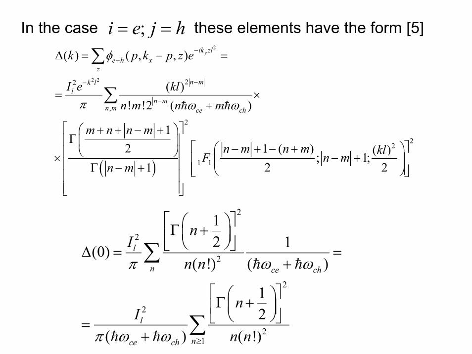
In the case these elements have the form [5];i e j h= =

( )

2

2 2 22

,

2

22

1 1

( ) ( , , )

( )! !2 ( )

12 1 ( ) ( ); 1;

2 21

yik zle h x

z

n mk ll

n mn m ce ch

k p k p z e

I e kln m n m

m n n mn m n m klF n m

n m

φ

π ω ω

−−

−−

−

Δ = − =

= ×+

⎡ ⎤⎛ + + − + ⎞Γ⎢ ⎥⎜ ⎟ ⎡ ⎤⎛ − + − + ⎞⎝ ⎠⎢ ⎥× − +⎢ ⎥⎜ ⎟⎢ ⎥Γ − + ⎢ ⎥⎝ ⎠⎣ ⎦⎢ ⎥⎢ ⎥⎣ ⎦

∑

∑

2

2

2

2

2

21

12 1(0)

( !) ( )

12

( ) ( !)

l

n ce ch

l

nce ch

nI

n n

nI

n n

π ω ω

π ω ω ≥

⎡ ⎤⎛ ⎞Γ +⎜ ⎟⎢ ⎥⎝ ⎠⎣ ⎦Δ = =+

⎡ ⎤⎛ ⎞Γ +⎜ ⎟⎢ ⎥⎝ ⎠⎣ ⎦=+

∑

∑

The chemical potential of the Bose-Einstein condensed magnetoexcitons in the HFBA equals to [5]:

where the renormalized ionization potential of magnetoexcitons is introduced:

μ

2

2

( ) 2 ( 2 ( ) )

( ) 2 ( 2 ( ) ( )),

HFBex ex l

ex

k v B A k II Ik v B A k E kI

μ = − + − + − =

− + − + Δ −

( )exI k

( ) ( ) ( );ex exI k I k k= + Δ ( ) ( );ex lI k I E k= − ( ) ( ).ex exE k I k= −

and the coefficients A, B are introduced as follows:

;i i e hA A A− −= = i iB B− =

The dependence of the chemical potential on the filling factor is determined by the coefficient [5]

HFBμ

2 2

2 ( ),( )

1 1

22

| |1 1

2

2 2

1 1

2 [ ( 1)!]2 ( )2 ! !( )

( )2 ! !( )

1( ) 1 ( )2 ( ; 1; )

( 1) 2 2

m n m nl m n

n mn mco

n mk ll

n mn mco

I A n mB A kn m n m

I e kln m n m

n m n mn m n m k lF n m

n m

π ω

π ω

+ ++

+≥ ≥

−−

−≥ ≥

− + −− +Δ =

+

+ ×+

⎡ + + − + ⎤Γ⎢ ⎥− + − +

× − +⎢ ⎥Γ − +⎢ ⎥

⎢ ⎥⎣ ⎦

∑∑

∑∑

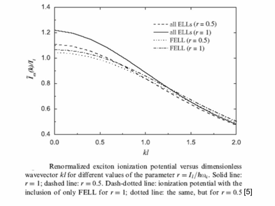
[5]

0.5l

ce

Irω

= =

1l

ce

Irω

= =

[5]

In the special cases we have

where

† †suppl

, ,

† † † †

, , , ,

1 ( , ; )2

(1)1 ( , ; ) ( , ; )2

e e p q q s p sp q s

h h p q q s p s e h p q q s p sp q s p q s

H p q s a a a a

p q s b b b b p q s a b b a

φ

φ φ

− + −

− + − − + −

= − −

− −

∑

∑ ∑

,

( , , ; , )( , , ) (2)

and( , , ; , ) ( ,0; ,0; , ; , )

(3)( , ; , ; ,0; ,0)

i ji j

n m ci cj

i j i jt

i j

p q z n mp q s

n m

p q z n m F p q p t n q t m

F p t n q t m p z q z

φφ

ω ω

φ

−−

− −

−

=+

= − + ×

× − + − +

∑

∑

( )

( )

2, ,

, ,

2

( , , ; , ) exp ( )

(4)exp ( ) ( ) ( ) and

e e t k z tt

n m n m

p q z n m W W i p q t l

i p q t z l t i t z i

σκ σ

φ κ

σ κ σ

− −

+ +

≅ − − ×

× − − − + − +

∑

The Hamiltonian of the supplementary interactions between electrons and holes lying on the LLLs [6].

The Hamiltonian (1) is a Hermitian conjugate form, if the requirements are fulfilled

The hermiticity requirement (7) can be deduced, for example, in the case of electron-electron interaction as follows

( )

( )2 2 2

2, ,

, ,

22

, , , , ,2 20

( , , ; , ) exp ( )( )

( ) ( ) ( ) ( ) , (5)where

2 , (6)

e h t k z tt

n m n m

s k l

s s k s k s k s k

p q z n m W W i p q l

t i t i t z i t z i

eW e W W W WS s k

σκ σ

κ

φ κ σ

κ κ σ σ

πε

− −

+−

− − − −

≅ + + ×

× + − − + − −

= = = =+

∑

* ( , ; ) ( , ; ), , , (7)i j i jp s q s s p q s i j e hφ φ− −− + − = =

* 2, ,

, ,

2

( , ; ; , ) exp( ( 2 ) )

exp( ( ) )( ) ( ) (8)

i i t z tt

n m n m

p z q z z n m W W i p q z t l

i p q t z l t i t z i

κ σκ σ

φ κ

σ κ σ

− − −

+ +

− + − = − − − − ×

× − − − − − + −

∑

Introducing the new summation variables [6]

and taking into account the properties (5) we will obtain exactly the expression (4), what proves the affirmation.

In the same way we can write:

which after the substitution (9) coincides with expression (5).There are another two properties of the coefficients namely their

reality and parity i.e.

They can be proved as was demonstrated above using the substitutionand , when the reality is considered and the substitution

when the parity is discussed

* 2, ,

, ,( , ; ; , ) exp( ( )( ) ) (10)

( ) ( ) ( ) ( )

e h t t zt

n m n m

p z q z z n m W W i p q l

t i t i t z i t z i

κ σκ σ

φ σ κ

κ κ σ σ

− +− + − = − + + ×

× − + + − + +

' , ', ' (9)t t z κ σ σ κ= − = − = −

∑

( , ; )i j p q sφ −

'σ σ= −'κ κ= −

', ' 't t andσ σ κ κ= − = − = −

* ( , ; ) ( , ; )

( , ; ) ( , ; ) (11)i j i j

i j i j

p q s p q s

p q s p q s

φ φ

φ φ− −

− −

=

− − − =

Side by side with three properties demonstrated above there is a another property related with the translational symmetry of the system in one in-plane direction which does exist in the Landau gauge description. As a result the coefficients do not depend separately on the variables p and q, but in their linear combination as follows [6]

( , ; )i j p q sφ −

-- ( , ; ) ( , ); ; (12)

( , ; ) ( , ); ;with the properties

i ii i

e he h

p q s s p q s

p q s s p q

φ φ κ κ

φ φ σ σ−−

= = − −

= = +

*

*

( , ) ( , );

( , ) ( , ); (13)

( , ) ( , )Their Fourier transforms are

i j i j

i j i j

i j i j

s s

s s

s s

φ σ φ σ

φ σ φ σ

φ σ φ σ

− −

− −

− −

− =

=

− − =

2( , ) ( , ) exp( ) (14)i ji j s s i lκ

ψ σ φ κ κσ−− =∑

Their symmetry properties follow directly from the previous ones [6]

These properties will be used below during the transformation of Hamiltonian the (1) written in the terms of the single particle operators to the form expressed through the two-particle operators of the electrons and holes densities of the type

*

*

*

( , ) ( , );

( , ) ( , );

( , ) ( , )

Their lead to the conclusion( , ) ( , ) (15)

i j i j

i j i j

i j i j

i j i j

s s hermiticity

s s reality

s s parity

s s

ψ σ ψ σ

ψ σ ψ σ

ψ σ ψ σ

ψ σ ψ σ

− −

− −

− −

− −

= − −

= −

− − =

=

† †, , ,p p p pa a b b( ) and ( )e hQ Qρ ρ

2

2

†

2 2

†

2 2

( )

( ) (16)

y

x x

y

x x

iQ tle Q Qt tt

iQ tlh Q Qt tt

Q e a a

Q e b b

ρ

ρ

− +

+ −

=

=

∑

∑

The relations between two sets of operators are [6]

Taking into account that

† 2

2 2

† 2 2

† 2 2

2

1 ( , ) exp( );

1 ( , ) exp ; (17)2

1 ( , ) exp ;2

where , S is the layer surface area and is the magnetic length.2

He

es sp p

ep p s

eq q s

a a s i plN

isa a s i pl lN

isa a s i ql lN

SN ll

κ

κ

κ

ρ κ κ

κρ κ κ

σρ κ σ

π

− +

−

+

= −

⎛ ⎞= − − +⎜ ⎟⎝ ⎠

⎛ ⎞= − −⎜ ⎟⎝ ⎠

=

∑

∑

∑

2

re the -symbol Kronecker was used1 exp( ( ) ) ( , ) (18)kr

p

ip lN

δ

σ κ δ σ κ− =∑

† †

, , ,

† †

1( , ; ) ( , ) ( , ) ( , ),

( , ; ) ( ,0) , (19)

; ;

e ee e p p s q q s e ep q s s

e ee e i is s

e h e hp p p pp p

p q s a a a a s s sN

p p s s s B

a a N b b N N N N

σ

φ ψ σ ρ σ ρ σ

φ φ

− − + −

−− −

= − −

− = =

= = = +

∑ ∑

∑ ∑

∑ ∑

and the similar expressions for the hole-hole interaction we can write [6]

† † † †

, , , ,

,

1 1( , ; ) ( , ; )2 2

1 1 ( , ) ( , ) ( , ) ( , ) ( , ) (20)2 2

The supplementary electron-hole interaction can be transformed a

e e p q q s p s h h p q q s p sp q s p q s

e e h hi i i is

p q s a a a a p q s b b b b

B N s s s s sN σ

φ φ

ψ σ ρ σ ρ σ ρ σ ρ σ

− + − − + −

− −

+ =

⎡ ⎤= − + − − + − −⎣ ⎦

∑ ∑

∑s follows

† †

, , ,

suppl,

1( , ; ) ( , ) ( , ) ( , ) (21)

As a result the full Hamiltonian (1) of the supplementary interaction has the form1 1 ( , ) ( , ) ( , )2 2

e he h p q q s p s e hp q s s

e ei i i is

p q s a b b a s s sN

H B N s s sN

σ

σ

φ ψ σ ρ σ ρ σ

ψ σ ρ σ ρ σ

− + − −

− −

= − − − −

= − − −

∑ ∑

∑

,

( , ) ( , )

1 ( , ) ( , ) ( , ) (22)

h h

e he hs

s s

s s sN σ

ρ σ ρ σ

ψ σ ρ σ ρ σ−

⎡ ⎤+ − − −⎣ ⎦

− − − − −∑

Instead of density operators for electrons and holes we can introduce their in-phase and in opposite-phase linear combinations [6]

where

ˆˆ ˆ ˆ ˆ ˆ( ) ( ) ( ); ( ) ( ) ( );1 1ˆ ˆˆ ˆ ˆ ˆ( ) ( ) ( ) ; ( ) ( ) ( ) (23)2 2

They lead to the following relations1ˆ ˆ ˆ ˆ ˆ ˆ( ) ( ) ( ) ( ) ( ) (2

e h e h

e h

e e h h

Q Q Q D Q Q Q

Q Q D Q Q D Q Q

Q Q Q Q Q

ρ ρ ρ ρ ρ

ρ ρ ρ ρ

ρ ρ ρ ρ ρ ρ

= − − = + −

⎡ ⎤ ⎡ ⎤= + = − − −⎣ ⎦ ⎣ ⎦

− + − = −

suppl

ˆ ˆ) ( ) ( ) ;

ˆ ˆˆ ˆ( ) ( ) ( ) ( ) ( ) (24)

ˆ ˆˆ ˆ( ) ( ) ( ) ( ) ( ) 0;

and to the final expression1 1 ˆ( )2 4

e hQ

e hQ

i iQ

Q D Q D Q

Q Q D Q D Q Q

Q Q D Q D Q Q

H B N V QN

ψ ρ ρ

ψ ρ ρ

ρ

−

−

−

⎡ ⎤+ −⎣ ⎦

⎡ ⎤− − − =⎣ ⎦

⎡ ⎤= − − − =⎣ ⎦

= −

∑

∑

∑ 1 ˆ ˆˆ( ) ( ) ( ) ( ) ( ) (25)4 Q

Q Q U Q D Q D QN

ρ − − −∑

( ) ( ) ( ); ( ) ( ) ( ); (26)i i e h i i e hU Q Q Q V Q Q Qψ ψ ψ ψ− − − −= + = −

( )†

1ˆ ˆ ˆ ˆ ˆ( ) ( )2

1 1 1 ˆ ˆˆ ˆ( ) ( ) ( ) ( ) ( ) ( )2 4 4

( ) ( )

e h e e h hQQ

i iQ Q

i i

W Q Q N N N N

B N V Q Q Q U Q D Q D QN N

N e d k e d kϕ ϕ

ρ ρ μ μ

ρ ρ

η

−

−

⎡ ⎤= − − − − − +⎣ ⎦

+ − − − − −

− +

∑

∑ ∑

H

( ( ) )v ( ( ) ( ) )v; ( ) ( ) ( ) ( ) ( );ex ex ex lE k E k k E k E k k I k E kη μ μ= − = − Δ − = − Δ = − − Δ +

22 [ ]( ) ( ); ( ) 2 ;

2z

ex l QQ

K Q lE k I E k E K W Sin⎛ ⎞×

= − + = ⎜ ⎟⎝ ⎠

∑

lIμ μ= + 2v ;v = 2v ;exN N=1( ) ( )

2QW Q W V QN

= −

2 21( ) ( , , ) ( ) exp( [ ] )yk sle h x e h z

s Q

k p p k s e Q i k Q lN

φ ψ−− −Δ = − − = ×∑ ∑

Generalized Hamiltonian taking into account the influence of the excited Landau levels and the broken gauge symmetry [6]

2

2

† †

[ ]ˆ ˆ( ) [ ( ), ] ( ( ) ( )) ( ) 2 ( ) ( ) ( )2

[ ]1 ( )( ) ( ) ( ) ( ,0) ;2

ˆ( ) [ ( ), ] ( ( )

z

Q

i izkr

Q

P Q ldi d P d P E P P d P i W Q Sin Q d P Qdt

P Q l D PU Q Cos D Q d P Q Ne P eN Ndi d P d P E Pdt

ϕ ϕ

μ ρ

η δ η

μ

⎛ ⎞×= = − + −Δ − − −⎜ ⎟

⎝ ⎠⎛ ⎞×

− − − +⎜ ⎟⎝ ⎠

− = − = − − + Δ

∑

∑

H

H †

2†

2†

( )) ( )

[ ] ˆ2 ( ) ( ) ( )2

[ ]1 ( )( ) ( ) ( ) ( ,0) ;2

z

Q

i izkr

Q

P d P

P Q li W Q Sin d P Q Q

P Q l D PU Q Cos d P Q D Q Ne P eN N

ϕ ϕ

ρ

η δ η− −

− − +

⎛ ⎞×+ − − − +⎜ ⎟

⎝ ⎠⎛ ⎞×

+ − − − + −⎜ ⎟⎝ ⎠

∑

∑

Equations of motion in the case of BEC on the state k=0 [6]

2

2

ˆˆ ˆ( ) [ ( ), ]

[ ] ˆ ˆ ˆ ˆ( ) [ ( ) ( ) ( ) ( )]2

[ ]( ) ( ) ( ) ( ) ( ) ;2 2

ˆˆ ˆ( ) [ ( ), ]

[ ]( )

z

Q

z

Q

z

Q

di P Pdt

P Q li W Q Sin P Q Q Q P Q

P Q li U Q Sin D P Q D Q D Q D P QNdi D P D Pdt

P Qi W Q Sin

ρ ρ

ρ ρ ρ ρ

= =

⎛ ⎞×= − − + − +⎜ ⎟

⎝ ⎠⎛ ⎞× ⎡ ⎤+ − + −⎜ ⎟ ⎣ ⎦⎝ ⎠

= =

×−

∑

∑

∑

H

H

2

2†

ˆ ˆˆ ˆ[ ( ) ( ) ( ) ( )]2

[ ] ˆ ˆˆ ˆ( ) [ ( ) ( ) ( ) ( )] 2 ( ) ( ) ;2 2

i iz

Q

l Q D P Q D P Q Q

P Q li U Q Sin D Q P Q P Q D Q N e d P e d PN

ϕ ϕ

ρ ρ

ρ ρ η −

⎛ ⎞− + − +⎜ ⎟

⎝ ⎠⎛ ⎞× ⎡ ⎤+ − + − + − −⎜ ⎟ ⎣ ⎦⎝ ⎠

∑

†11

† †12

†13

†14

ˆ( , ) ( , ); ( ,0) ;

ˆ( , ) ( , ); ( ,0) ;

ˆ ( , ) ˆ( , ) ; ( ,0) ;

ˆ ( , ) ˆ( , ) ; ( ,0) ;

G P t d P t X P

G P t d P t X P

P tG P t X PN

D P tG P t X PN

ρ

=

= −

=

=

†11

† †12

†13

†14

ˆ( , ) ( ) ( ) ;

ˆ( , ) ( ) ( ) ;

ˆ ( ) ˆ( , ) ( ) ;

ˆ ( ) ˆ( , ) ( ) ;

G P d P X P

G P d P X P

PG P X PN

D PG P X PN

ω

ω

ω

ω

ω

ω

ρω

ω

=

= −

=

=

[ ]ˆ ˆ( ) ( ); (0) ( ) ( ), (0) ;

ˆ ˆ( ) ;ˆ ˆ ˆˆ ˆ ˆ,

iHt iHt

G t A t B i t A t B

A t e Ae

A B AB BA

θ

−

= = −

=

⎡ ⎤ = −⎣ ⎦

ˆ ˆ( ) ( ); (0) ( ) (0), (0) ( ); (0)

ˆ ˆ ˆ( ) ( ), ; (0)

d d di G t i A t B t A B i A t Bdt dt dt

t C A t H B

δ

δ

⎡ ⎤= = + =⎣ ⎦

⎡ ⎤= + ⎣ ⎦

0 0

( ) ( ) ( )

ˆ ˆ ˆ( ) ( ) ( ), ; (0)

i t ti t i t t

i t

dG t dG t dedte i i dte i dtG tdt dt dt

i G C dt A t H B e

ω δω ω δ

ωω δ ω

∞ ∞ ∞ −−

−∞

∞

−∞

= = − =

⎡ ⎤= + = + ⎣ ⎦

∫ ∫ ∫

∫

2

1

2

4

2†

2

[ ]( ( ) ( )) ( , ) 2 ( ) ( ) ( )2

[ ]1 ( ) ( ) ( ) ( , ) ;2

[ ]( ( ) ( )) ( , ) 2 ( ) ( ) ( )2

1

z

Q

iz

Q

z

Q

P Q li E P P G P C i W Q Sin Q d P Q X

P Q lU Q Cos D Q d P Q X G P eN

P Q li E P P G P C i W Q Sin d P Q Q X

dN

ω

ϕω

ω

ω δ μ ω ρ

η ω

ω δ μ ω ρ

⎛ ⎞×+ + − + Δ = − − −⎜ ⎟

⎝ ⎠⎛ ⎞×

− − +⎜ ⎟⎝ ⎠

⎛ ⎞×+ − + − −Δ − = + − − − +⎜ ⎟

⎝ ⎠

+

∑

∑

∑

†4

2

3

2

2

4

( ) ( ) ( , ) ;

[ ] ( ) ( ) ( ) ( )( ) ( , ) ( )2

[ ] ( ) ( ) ( ) ( )( ) ;2 2

[ ] ( )( ) ( , ) ( )2

i

z

Q

z

Q

z

Q

P Q D Q X G P e

P Q l P Q Q Q P Qi G P C i W Q Sin XN N

P Q li D P Q D Q D Q D P QU Q Sin XN N N

P Q l D Qi G P C i W Q Sin

ϕ

ω

ω

ω

η ω

ρ ρ ρ ρω δ ω

ρω δ ω

−− − − −

⎛ ⎞× − −+ = − + +⎜ ⎟

⎝ ⎠

⎛ ⎞× − −+ +⎜ ⎟

⎝ ⎠

⎛ ⎞×+ = − ⎜ ⎟

⎝ ⎠

∑

∑

∑2

1 2

( ) ( ) ( )

[ ] ( ) ( ) ( ) ( )( )2 2

2 ( , ) ( , ) ;

z

Q

i i

P Q D P Q Q XN N

P Q li D Q P Q P Q D QU Q Sin XN N N

e G P e G P

ω

ω

ϕ ϕ

ρ

ρ ρ

η ω ω−

− −+ +

⎛ ⎞× − −+ + +⎜ ⎟

⎝ ⎠

⎡ ⎤+ −⎣ ⎦

∑

22 2

11 2

21

2 2

31 2

[ ]( )2( ) ( )

( , ) ( ) ( ) ;( ) ( )

( , ) 0;

[ ] [ ]( ) ( )( ) ( ) 2 2( , )

Q P

Q P

P Q lU Q CosD A D A

P i E P PN i E P Q P Q

P

P Q l P Q lU Q U Q P Cos SinD A d A NP i

N i E

ω ω δ μω δ μ

ω

ωω δ μ

≠

≠

⎛ ⎞×⎜ ⎟− ⎝ ⎠∑ = + + − + Δ −

+ + − − + Δ −

∑ =

⎛ ⎞ ⎛ ⎞× ×− ⎜ ⎟ ⎜ ⎟− ⎝ ⎠ ⎝ ⎠∑ =+ + −

∑

∑2

2

41

2

;( ) ( )

[ ]( )( ( ) ( ))( ) ( ) 2(0)( , ) ( ) 2

( ) ( )

( ) ( )

i

Q P

Q

P Q P Q

P Q lW Q U P U Q P SinD A d A NdP e U P

N i E P Q P QN

D A d A N

N

ϕω ηω δ μ≠

− + Δ −

⎛ ⎞×− − ⎜ ⎟− ⎝ ⎠∑ = − + + −+ + − − + Δ −

−−

∑2

2 [ ]( ) ( )2

;( ) ( )P

P Q lU Q U P Cos

i E P Q P Qω δ μ≠

⎛ ⎞×⎜ ⎟⎝ ⎠

+ + − − + Δ −∑12

22

22 2

2 2

†

32 2

( , ) 0;

[ ]( ) ( )2( ) ( )

( , ) ( ) ( ) ;( ) ( )

[ ] [ ]( ) ( )( ) ( ) 2 2( , )

Q P

Q P

P

P Q lU Q U Q CosD A D A

P i E P PN i E P Q P Q

P Q l P Q lU Q U Q P Cos Sind A D A NP i

N

ω

ω ω δ μω δ μ

ω

≠−

≠−

∑ =

⎛ ⎞×− ⎜ ⎟− ⎝ ⎠∑ = + − + −Δ − −

+ − + − − −Δ − −

⎛ ⎞ ⎛× ×− − ⎜ ⎟ ⎜− ⎝ ⎠ ⎝∑ =

∑

∑2

2††

42

;( ) ( )

[ ]( )( ( ) ( ))( ) ( )(0) 2( , ) ( ) 2

( ) ( )

i

Q P

i E P Q P Q

P Q lW Q U Q P U P Sind A D A NdP e U P

N i E P Q P QNϕ

ω δ μ

ω ηω δ μ

−

≠−

⎞⎟⎠

+ − + − − − Δ − −

⎛ ⎞×− − − ⎜ ⎟− ⎝ ⎠∑ = − − − −+ − + − − −Δ − −∑

22

†

2

[ ]( ) ( )( ) ( ) 2 ;

( ) ( )Q P

P Q lU Q U P Cosd A D A N

N i E P Q P Qω δ μ≠−

⎛ ⎞×− ⎜ ⎟− ⎝ ⎠−+ − + − − −Δ − −∑

13

23

22

33 2

43

( , ) 0;

( , ) 0;

( ) ( ) [ ]( , ) ( )( ( ) ( )) ;( ) 2

( , ) 0;Q P

P

P

D A D A P Q lP i U Q U Q U Q P SinN i

P

ω

ω

ω ω δω δ

ω≠

∑ =

∑ =

⎛ ⎞− ×∑ = + − − − − ⎜ ⎟+ ⎝ ⎠∑ =

∑

14

24

34

22

44

2

( , ) 2 ;

( , ) 2 ;

( , ) 0;

2 ( ) ( ) [ ]( , ) ( )( ( ) ( ))( ) 2

( ) ( ) ( )( ( )

( )

i

i

Q P

Q P

P e

P e

P

D A D A P Q lP i W Q U Q P U P SinN i

D A D AU Q U P

N i

ϕ

ϕ

ω η

ω η

ω

ω ω δω δ

ω δ

−

≠−

≠

∑ = −

∑ =

∑ =

⎛ ⎞− ×∑ = + − − − +⎜ ⎟+ ⎝ ⎠

−+

+

∑

∑2

2 [ ]( )) ;2

P Q lU Q Sin⎛ ⎞×

− − ⎜ ⎟⎝ ⎠

2 2

† 3

†

( ) ( ) 4 ;

( ) ( ) ( ) ( ) 2 ;

(0) (0) ;

D Q D Q u v N

D Q d Q N d Q D Q N uv N

d d uv N

− =

− = − = −

= =

33( ; ) 0;P ωΣ =

11 22 44

41 22 14

42 11 24

( ; ) ( ; ) ( ; )

( ; ) ( ; ) ( ; )

( ; ) ( ; ) ( ; ) 0

P P P

P P P

P P P

ω ω ω

ω ω ω

ω ω ω

Σ Σ Σ −

−Σ Σ Σ −

−Σ Σ Σ =

The energy spectrum of elementary excitations of magnetoexcitonsin the case when concentrations corrections haven’t been taken into

account, the filling factor equals to zero [6].

0.0 0.5 1.0 1.5 2.0 2.5 3.0

-0.6

-0.4

-0.2

0.0

0.2

0.4

0.6

pl

ÑwêI l

11

41

22

†

42

14

24

442

3

( , ) ( ) ( );(0)

( , ) ( ) ;

( , ) ( ) ( );

(0)( , ) ( ) ;

( , ) 2 ;

( , ) 2 ;

( , ) ;

(0) 2 ( 2 (0));

( (0) ) 2 (i i i i

P E P Pd

P U PN

P E P P

dP U P

NP

P

P i

v B A

v v B

σ ω ω μ

σ ω η

σ ω ω μ

σ ω η

σ ω η

σ ω η

σ ω ω δ

μ

η μ− −

= + − + Δ

= − +

= − + −Δ −

= − −

= −

=

= +

= −Δ + − + Δ

= − Δ + = −2 2

2 2

2 (0));

( ) (0); 0; 0; ( ) (0) , (0) 2

i i i i

P l

i i

A

P k v U P U e U A

− −

−

−

− + Δ

Δ ≈ Δ = ≠ ≅ =

The dispersion equation in this case looks as [6]

( )2 ( ) (0)( ) (0) 4

U P dE P

Nω μ η η

⎛ ⎞= ± − + Δ + −⎜ ⎟⎜ ⎟

⎝ ⎠

In the Ref [ ] the coefficient 1( 2 (0))i i i il

B AI− −− + Δ was determined

at the ratio 12

lIrω

= = as equal to 0,025. It was used in the present

calculations leading to the main parameters μ and η

2 2( (0)) 2 0,025 0,05 ,l

v vI

μ + Δ= =i 3 3( (0)) 2 0,025 0,05

l

v v vI

μη + Δ= − = − = −i

and(0) (0) 2 0,15 .i i

ll

U d A uv uvII N−= =

( )2 2

22 2 2 20,05 ( ) 0, 2 0,05 0,15P l

v E P v v uveω−⎛ ⎞

= ± − + +⎜ ⎟⎜ ⎟⎝ ⎠

Introducing the dimensionless energies

/ lIω ω= and ( ) ( ) / lE P E P I= one can transcribe the solution as follows

Two exciton branches of the energy spectrum of collective elementary excitations of the Bose-Einstein condensed

magnetoexcitons on the wave vector , calculated in HFBAusing the self-energy parts [6] and the filling factor 2 0,1.v =

0k =

Two exciton branches of the energy spectrum of collective elementary excitations of the Bose-Einstein condensed

magnetoexcitons on the wave vector , calculated in HFBA,using the self-energy parts [6] and the filling factor

0.0 0.5 1.0 1.5 2.0 2.5

-0.6

-0.4

-0.2

0.0

0.2

0.4

0.6

pl

ÑwêI l

0k =2 0,1.v =

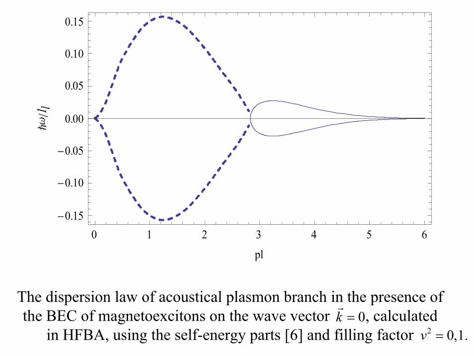
The dispersion law of acoustical plasmon branch in the presence of the BEC of magnetoexcitons on the wave vector , calculated

in HFBA, using the self-energy parts [6] and filling factor

0 1 2 3 4 5 6-0.15

-0.10

-0.05

0.00

0.05

0.10

0.15

pl

ÑwêI l

0k =2 0,1.v =

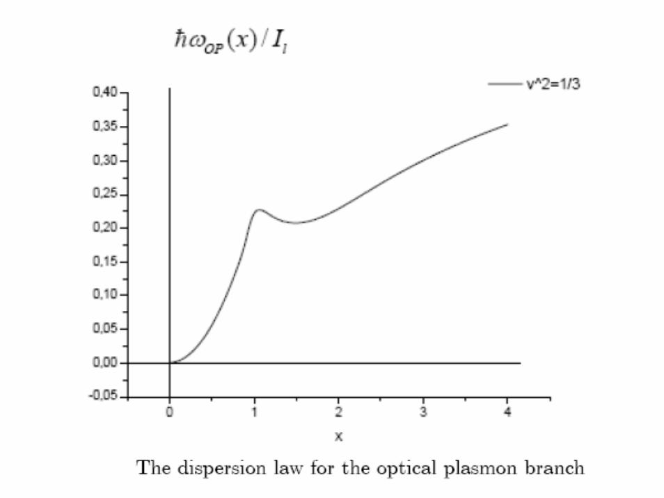
The dispersion law of optical plasmon branch in the presence of the BEC of magnetoexcitons on the wave vector , calculated in

HFBA, using the self-energy parts [6] and the filling factor

0.0 0.5 1.0 1.5 2.0 2.5 3.00.00

0.05

0.10

0.15

pl

ÑwêI l

0k =2 0,v = 1.

The comparison of the energy per one particle in the frame of four different ground states: Incompressible quantum liquid (IQL); Charge-density wave (CDW); Electron-hole liquid (EHL) and Metastable dielectric liquid

(MDL) formed by Bose-Einstein condensed magnetoexcitons [7].

1/ 5v = 1/ 3v = 2vv =

Ene

rgy

per o

ne p

artic

le

Formation of composite

bosons and composite

fermions [7]

( ) ( )

( )

( )

( ) ( )

( )

22

22

2

2 22

4( , )

[ ]( ) ( ) ( ) ( ) ( )2

[ ]1 ( )( ( ) ( )) ( ) ( ) ;2

4( , )

1 1( ) ( ) ( ) ( ) ( ) ( )4 2

OP

z

Q

z

Q

AP

Q

P ii

P Q lW Q W Q W Q P Sin Q Q

P Q lU Q U Q U Q P Sin D Q D QN i

P ii

W Q U Q W Q U Q P W Q P U QN N

Si

ω ω δω δ

ρ ρ

ω δ

ω ω δω δ

Σ = + − ×+

⎛ ⎞×× − − − −⎜ ⎟

⎝ ⎠⎛ ⎞×

− − − −⎜ ⎟+ ⎝ ⎠

Σ = + − ×+

⎡ ⎤× + + − + − ×⎢ ⎦⎣

×

∑

∑

∑2

2 [ ] ( ) ( )2

1( ) ( )2

z

Q

P Q ln Q Q

W Q W V QN

ρ ρ⎛ ⎞×

−⎜ ⎟⎝ ⎠

= −

Optical and acoustical plasmons in the electron-hole liquid (EHL) state, taking into account the excited Landau levels (ELLs).

Plasmon frequency:

3D:

2D:

2 ( ) 2p e k kk N T Vω =

2 2

;2kkTm

=2

20

4 ;keVVkπ

ε= ;eNn

V=

22

0

4 ;epe nm

πωε

=

2 2

;2kkTm

=2

0

2 ;keVSkπε

= ;eSNnS

=2

2

0

2 ;Sp

e n qm

πωε

=

( )p q qω ∼

The dispersion law for the acoustical plasmon branch:

( )2

2 2 [ ] ˆ ˆ( ) ( ) ( )2

zQ Q P Q

Q

P Q lW W W Sin Q Qω ρ ρ+

⎛ ⎞×= − −⎜ ⎟

⎝ ⎠∑

22 2 2 [ ] ˆ ˆ( ) ( ) ( )

2z

QQ

P Q lW Sin Q Qω ρ ρ⎛ ⎞×

= −⎜ ⎟⎝ ⎠

∑

ˆ ˆ( ) ( )Q Qρ ρ −The average is calculated, when the ground state represents the EHL

† † 2p p p pa a b b v= =

The dispersion law for the optical plasmon branch:

2 2ˆ ˆ( ) ( ) 2 (1 )

ˆˆ ( ) ( ) 0

Q Q Nv v

Q D Q

ρ ρ

ρ

− = −

− =

2D electron-hole system in a strong perpendicular magnetic field and a lateral electric field

;dEV cH

=

ˆ ˆ ˆ ˆ[ ( ), ( )] [ ( ), ( )]E ED Q D P D Q D P=

, ,( , ) ( )ipx

i ip n p n

x

ex y yL

ψ ϕ=2

, 0 2

( )1( )2

ipi

p n

y yy Exp

llϕ

π=

⎡ ⎤−= −⎢ ⎥

⎢ ⎥⎣ ⎦

2 ;i i i dpq mVy l pe

⎛ ⎞= − +⎜ ⎟⎝ ⎠

, ; ii e h q e= = ±

( )2

,1 ;22

i i dp n d ci

mVE V p nω= − + + +

ˆ ˆ ˆ ˆ[ ( ), ( )] [ ( ), ( )];E EQ P Q Pρ ρ ρ ρ=

( ) ( );

;

( ) ( ) ; ( );

y eiQ uEe e

di

ci

E E Ee h

Q e QVu

Q Q Q

ρ ρ

ω

ρ ρ ρ

−=

=

= − −

( ) ( );

;

( ) ( ) ( );

y hiQ uEh h

cii

E E Ee h

Q e QeHm c

D Q Q Q

ρ ρ

ω

ρ ρ

−=

=

= + −

2 2 2

00

(1 )2 2e v vcε

−=

0† †

0

0

2

ˆ ˆ ˆ ;

( );

1ˆ ˆ ˆˆ ˆ( ) ( ) ) ;2

ˆ ˆ[ ( ), ] ( );

ˆ ˆ( ) ( )

[ ] ˆ ˆ ˆ ˆ[ ( ) ( ) ( ) ( )2

E ECoul

d p p p pp

E E ECoul e eQ

Q

E Ed x

E Ed x

E E E EzQ

Q

H H H

H V p a a b b

H W Q Q N N

Q H V Q Qdi P V P Pdt

P Q li W Sin Q P Q P Q Q

ρ ρ

ρ ρ

ρ ρ

ρ ρ ρ ρ

= +

= +

⎡ ⎤= − − −⎣ ⎦

=

= −

⎛ ⎞×− − + −⎜ ⎟

⎝ ⎠

∑

∑

∑ ]

which leads to the previous self-energy parts, in which the frequency is substituted by

The drift velocity is less than the velocity c0at the condition

( )Pω ( ) d xP V Pω −

400; 2 10d

cV c E H Hc

−< < ≈ ⋅

Composite fermions and bosons in 2D e-h system with filling factor v=1/2

612

62e h

N

NN N

ν

=

=

= = =