Exchange Rate Pass-Through in Brazil: a Markov Switching ... de Economa/PORTUGAL... · example,...

1

Exchange Rate Pass-Through in Brazil: a Markov Switching DSGE

Estimation for the Inflation Targeting Period (2000-2015)

Fabrizio Almeida Marodina, Marcelo Savino Portugal

b

a Department of Economics, University of California Irvine, 3151 Social Sciences Plaza, Irvine, CA, 92697-5100,

United States of America. E-mail: [email protected]

a,b Graduate Program in Economics (PPGE), Universidade Federal do Rio Grande do Sul, Av Joao Pessoa 52 /

suite 33B, Porto Alegre, RS, 90040-000, Brazil. E-mail: [email protected]

Abstract: This paper investigates the nonlinearity of exchange rate pass-through in the Brazilian

economy during the floating exchange rate period (2000-2015) using a Markov-switching DSGE

(MS-DSGE) model. We apply the methods proposed by Baele et al. (2015) and a basic new

Keynesian model, with the addition of new elements to the AS curve and a new equation for the

exchange rate dynamics. We find evidence of two distinct regimes for the exchange rate pass-

through and for the volatility of shocks to inflation. Under the so-called “normal” regime, the

long-run pass-through to consumer prices inflation is estimated at 0.00057 percentage points,

given a 1% exchange rate shock. Comparatively, the expected pass-through under a “crisis”

regime is of 0.1035 percentage points to inflation, for the same exchange rate shock. The MS-

DSGE model outperforms the fixed parameters model according to several comparison criteria.

The results allowed us to identify the occurrence of three distinct cycles for the exchange rate

pass-through during the inflation targeting period in Brazil.

Keywords: Exchange-rate pass-through, DSGE Models, Regime Switching, Markov Chain.

JEL codes: E31, F31, C3.

2

1. Introduction

This paper assesses the exchange rate pass-through to inflation in the Brazilian economy

during the floating exchange rate period using a Markov-switching dynamic stochastic general

equilibrium (MS-DSGE) model. Our aim is to check for nonlinear behaviour of the exchange

rate pass-through, given the possibility it could further amplify inflation during external sector or

currency crisis.

The research is aligned with the recent literature in structural parameter drifting, or

nonlinear behavior of structural parameters. According to Hamilton (2014), nonlinear

mechanisms that trigger macroeconomic regime shifts are some of the most noteworthy

contemporary issues in macroeconomics. Current economies are subject to remarkable changes,

recurrent crises, recessions, and financial stress. These events produce “dramatic breaks” in

macroeconomic time series and, consequently, lead agents to create expectations under different

regimes.

Our motivation derives from the risk of underestimating the effect of an exchange rate

shock to inflation, specially under large devaluation events. The international literature has found

some meaningful evidence of nonlinear exchange rate pass-through, as we will further explore. If

that has been the case for the Brazilian economy, even after the adoption of the inflation

targeting regime, the researchers or policymakers may be incurring in a greater than expected

forecast error. Indeed, we sustain that the forecast error would be even greater during external

sector crisis, where policy decisions are of the highest importance.

The traditional approach to analyze changes in structural parameters is based on

Hamilton’s (1989) business cycle model. In this method, some parameters chosen in each

regression vary freely according to Markov processes. Sims & Zha (2006), for instance,

conducted a seminal work on regime shifts in the U.S. monetary policy by proposing and

estimating a structural MS-VAR model. However, the theoretical and empirical advances of

DSGE models, as well as their broad use in the analysis of economic policies, naturally arouse

interest in expanding the scope of these models so as to include regime-switching mechanisms.

The international literature is rife with several examples related to MS-DSGE models and

with solution and estimation methods. Justiniano & Primicieri (2008), for example, assess

regime switching in the volatility of shocks whereas Fernández-Villaverde, Guerrón-Quintana &

Rubio-Ramírez (2010), Bianchi (2013), Baele et al. (2015), and Iboshi (2016) focus on changes

in the Taylor rule parameters and their consequences for macroeconomic equilibrium. Authors

are usually keen on identifying periods during which the U.S. monetary policy has an “active”

vs. a “passive” behavior towards inflation.

Regarding solution methods for Markov-switching rational expectations models, major

contributions are given by Farmer, Waggoner & Zha (2009, 2011). These authors develop a set

of necessary and sufficient conditions for equilibria to be determinate, as well as an algorithm to

check these conditions in practice. Liu & Mumtaz (2010), and later Choi & Hur, (2015) rely on

the solution proposed by Farmer, Waggoner & Zha (2011) and utilize Bayesian estimation

methods in empirical studies on regime switching in monetary policy rules for the UK and South

Korea, respectively. More recently, Foerster et al. (2014) have proposed a new estimation

method, which uses perturbations to approximate solutions to nonlinearized MS-DSGE models,

for which Maih (2015) presents a practical implementation.

3

In Brazil, nearly all the estimated DSGE models have constant parameters, as in Silveira

(2008), Furlani, Portugal & Laurini (2010), Castro et al. (2011), and Palma & Portugal (2014).

An exception is Gonçalves, Portugal & Arágon (2016), who use the open-economy model

proposed by Justiniano & Preston (2010), the solution methods of Farmer, Waggoner & Zha

(2011), and a Bayesian estimation method similar to that of Liu & Mumtaz (2010). The authors

find a superior fit of an MS-DSGE model with changes in the Taylor rule parameters and in

volatility of shocks, comparatively to fixed parameters models.

On the other hand, there are several studies that investigate changes in structural

parameters of the Brazilian economy by applying conventional regime switching models such as

Hamilton (1989). Fasolo & Portugal (2004), for instance, find changes in the Phillips curve

parameters whereas Vieira & Pereira (2013) describe differences in the business cycle dynamics.

More recently, Rodrigues & Mori (2015) have identified different monetary policy regimes using

a model with changes in the Taylor rule parameters, and Oliveira & Feijó (2015) have

investigated the nonlinearity between unemployment and inflation using a Phillips curve with

Markov switching.

We therefore assume that the paucity of empirical studies on MS-DSGE models in Brazil

is due mainly to their recent development rather than to the belief that our economy is subject to

fixed structural parameters. Hence, we understand that our investigation into regime switching in

the exchange rate pass-through parameter should be conducted by employing this class of

models in order to contribute to their dissemination and improvement.

The variable, or nonlinear, behavior of the exchange rate pass-through is theoretically

endorsed by arguments from Dixit (1989) and Taylor (2000). Dixit (1989) attributes the

differences in pass-through to firms decision-making uncertainty. According to him, the more

uncertain the steady state of the exchange rate, the greater the incentive for firms to adopt a

waiting strategy before making the decision to adjust prices, given adjustment (menu) and

reputation costs, if the firm needs to reverse its decision. Thus, if the exchange rate shock is seen

as permanent, agents would respond with a higher pass-through to prices, compared to cases of

temporary shocks. Dixit’s (1989) assumption is part of an approach that considers the pass-

through to be incomplete as a result of firms’ behavior and of market prices denominated in local

currency, which Razafindrabe (2016) calls “positive approach.” Larue, Gervais & Rancourt

(2010), for instance, provide microeconomic evidence in favor of this assumption, relating menu

cost to different levels of incomplete pass-through.

Taylor (2000), however, sustain that differences in the level of pass-through are related to

price rigidity. In periods of higher inflation, firms transfer their costs more frequently, including

costs associated with imported inputs, as overall price rigidity is smaller. Razafindrabe (2016)

clarifies that nominal price rigidity of imported goods is the main explanation to incomplete

pass-through under the so-called normative approach. The author introduces a DSGE model in

which the problem with optimal price adjustment by importing firms, through a Calvo (1983)

mechanism, causes a deviation from the law of one price and, therefore, incomplete exchange

rate pass-through to inflation. Figueiredo & Gouvea (2011) support this viewpoint by giving

empirical evidence of heterogeneity in the pass-through between disaggregated prices negatively

linked to the level of price rigidity. Also, the DSGE model proposed by Choudhri & Hakura

(2015) is based on price rigidity to explain the differences in the level of pass-through between

the prices of imported and exported goods. Besides providing a theoretically consistent

explanation, the authors manage to reproduce some characteristics of time series observed for

several countries.

4

From an empirical standpoint, variable or nonlinear exchange rate pass-through has been

investigated by the literature, but, in the case of Brazil, not within the DSGE framework. For

example, Goldfajn & Werlang (2000) confirm that the intensity of pass-through in cases of

exchange rate depreciation is not fixed, but depends upon a series of economic state variables.

The key factors would be the cyclical component of output, the initial overvaluation of the real

exchange rate, the initial inflation rate, and the level of economic openness. In the Brazilian

economy, Albuquerque & Portugal (2005) asseverate that the intensity of exchange rate pass-

through varies over time and depends on macroeconomic factors, which is also supported by

Tombini & Alves (2006). Minella et al. (2003) and Kohlscheen (2010) affirm that exchange rate

volatility is associated with variance of inflation and with higher pass-through. Moreover, the

nonlinear or asymmetric behavior of exchange rate pass-through is verified in the empirical

studies undertaken by Correa & Minella (2006), Nogueira Jr (2010), and Pimentel, Modenesi &

Luporini (2015).

In other countries, Holmes (2009) and Khemiri & Ali (2012) assess regime switching in

exchange rate pass-through by means of regressions based on the Phillips curve for New Zealand

and Tunisia, respectively. Donayre & Panovska (2016) gather strong evidence of nonlinear

behavior between the pass-through and economic activity for Canada and Mexico in a Bayesian

threshold VAR model. In particular, the authors find a higher pass-through in expansionary

periods, corroborating again Goldfajn & Werlang (2000). The influence of the macroeconomic

environment and of inflation stability on the observation of smaller pass-throughs is also

advocated by Winkelried (2014) in an empirical study for Peru.

In this paper, our goal is to estimate a basic new Keynesian model subject to regime

switching in the exchange rate pass-through parameter and in the volatility of shocks to inflation

by applying the methods developed by Baele et al. (2015). One of the peculiarities of this

method is the use of survey data on market expectations, making the estimation of the MS-

DSGE model easier. At the same time, Baele et al. (2015) suggest Cho’s (2014) recursive

solution method for regime switching rational expectations models, which circumvents some

problems of convergence observed in Farmer, Waggoner & Zha (2011). Our study differs from

that of Baele et al. (2015), who investigate regime switching in the monetary policy rule, as our

focus lies in the exchange rate pass-through. To achieve that, we expand the original model by

adding new elements to the AS curve and a new equation for exchange rate dynamics.

The MS-DSGE model estimation allows us to identify two possible regimes for the

exchange rate pass-through and the volatility of shocks to inflation. During a “normal” cycle, the

expected long-run pass-through is of 0.00057 percentage points to consumer prices inflation,

given a 1% exchange rate shock. Comparatively, the expected effect during a “crisis” cycle is

much higher, of 0.1035 percentage points to inflation, given the same exchange rate shock. In

addition, we verified that the volatility of shocks to inflation is larger during the “crisis” period.

The MS-DSGE model outperforms the linear model according to several comparison criteria.

We therefore understand that the results are useful to enrich models of inflation forecasting and

economic policy analysis.

The paper is organized into five sections, apart from this introduction. Section 2 describes

the basic new Keynesian model and its extensions, introduce regime switching, assess the

equilibrium conditions and presents our identification strategy. Section 3 presents the data and

the estimation method. Section 4 describes the results and their implications. Finally, Section 5

makes the concluding remarks.

5

2. The Model

This section describes the basic macroeconomic model, with the introduction of

exogenous exchange rate shocks. We expand the model by adding a regime-switching

mechanism. Then, we assess the rational expectations equilibrium and finally describe the

strategy for including survey expectations.

2.1 The new Keynesian model

Let us first consider the following macroeconomic new Keynesian structural model with

three variables and three equations, which is a benchmark for research in this area and was used

by Baele et al. (2015).

𝜋𝑡 = 𝛿𝐸𝑡𝜋𝑡+1 + (1 − 𝛿)𝜋𝑡−1 + 𝜆𝑦𝑡 + 𝜖𝜋,𝑡 𝜖𝜋,𝑡~𝑁(0, 𝜎𝐴𝑆2 ) (1a)

𝑦𝑡 = 𝜇𝐸𝑡𝑦𝑡+1 + (1 − 𝜇)𝑦𝑡−1 − 𝜙(𝑖𝑡 − 𝐸𝑡𝜋𝑡+1) + 𝜖𝑦,𝑡 𝜖𝑦,𝑡~𝑁(0, 𝜎𝐼𝑆2 ) (2)

𝑖𝑡 = 𝜌𝑖𝑖𝑡−1 + (1 − 𝜌𝑖)[𝛽𝐸𝑡𝜋𝑡+1 + 𝛾𝑦𝑡] + 𝜖𝑖,𝑡 𝜖𝑖,𝑡~𝑁(0, 𝜎𝑀𝑃2 ) (3)

We follow the notation of Baele et al. (2015) where 𝜋𝑡 is the inflation rate, 𝑦𝑡 is the

output gap and 𝑖𝑡 is the nominal interest rate. The operator 𝐸𝑡 refers to conditional expectations.

Each equation is amenable to unexpected shocks, respectively: 𝜖𝜋,𝑡 is the aggregate supply shock

(AS shock); 𝜖𝑦,𝑡 is the aggregate demand shock (IS shock); 𝜖𝑖,𝑡 is the monetary policy shock

(MP shock).

As to the structural parameters of the model, 𝛿 and 𝜇 stand for the forward-looking

behavior of firms (AS curve) and consumers (IS curve), respectively. The model allows for

endogenous persistence if these parameters are different from 1, with weight attached to the past

values of each variable. Parameter 𝜆 is the response of inflation to the output gap whereas 𝜙 is

the response of output to the real interest rate. The monetary authority’s reaction function is a

Taylor rule with smoothing parameter 𝜌𝑖, which reacts to inflation expectation with response 𝛽

and to deviations in output gap with parameter 𝛾. It is assumed that the monetary policy should

not react to temporary shocks, which affect only the current inflation rate without affecting its

future path.

The equations presented in this simple DSGE model are derived from the first-order log-

linearized conditions of the optimization problems of each representative agent: consumers,

firms, and monetary authority. A thorough description of the microfoundations of the basic new

Keynesian model can be seen in Galì (2008) or Romer (2011). The model describes the

dynamics of endogenous macroeconomic variables, in which current decisions are a function of

future expectations for these variables and their past values. As a closed economy model, it does

not deal with exchange rate pass-through. We found two alternatives to circumvent this problem.

The first option would be to add the full dynamics of a small open economy to the model,

as proposed by Adolfson et al. (2007), to estimate the incomplete pass-through. In this case, the

model is expanded to include nominal rigidity in the import and export sectors, the Phillips curve

is decomposed into domestic price and imported price curves, and capital, investment,

6

government sector, in addition to prices, output, and external interest rate, are included. We

would naturally also add the regime-switching parameters, and the transition probabilities. This

results in a complex model with dozens of parameters to be estimated or calibrated.

Since our focus is on the effect of pass-through during the floating exchange rate period

in Brazil, we have a relatively short time series and, therefore, we prefer to opt for a less

complex modeling strategy. We decided to model exchange rate shock as an observable

“demand shock” to non-produced inputs. So, we were inspired by Blanchard & Galí (2007), who

included a demand shock in the Phillips curve – called ∆𝑚.

We are aware that we are choosing to prioritize the direct effects on inflation of the

adjustment of input prices, as a consequence of exchange rate fluctuations. Therefore, we are

disregarding the indirect effects on aggregate demand, such as the change in the relative prices of

domestic and imported goods, the effect on the domestic interest rate, and the possibility of a

wealth effect. Our decision is justifiable for at least two reasons. First, exchange rate

depreciations in relatively closed economies, just as Brazil, tend to cause a relatively smaller

change in spending on domestic and imported goods. This argument is advocated by

Albuquerque & Portugal (2005) and also discussed in the empirical findings of Goldfajn &

Werlang (2000). Second, the estimation of a model with multiple regimes and small observed

time series would be hindered if the number of parameters increased considerably. In what

follows, we then describe the argument used by Blanchard & Galí (2007) to include a demand

shock in the new Keynesian Phillips curve.

Blanchard & Galí (2007) demonstrate that the optimizing behavior of consumers and

firms in an environment with real wage rigidity and price rigidity similar to that of the Calvo

(1983) model implies the following equilibrium relationship between inflation and output gap.

We keep the original notation used by the authors, which differs from that shown in our

equations (1)-(3).

𝜋𝑡 = 𝛿𝐸𝑡𝜋𝑡+1 + Φ1𝑥1𝑡 − Φ2[∆𝑚𝑡 + (1 + 𝜙)−1Δ𝜉]

In this equation, 𝑥1 is a linear combination between output gap - relevant for the current

welfare - and its lagged terms. The demand shock is represented by ∆𝑚 while Δ𝜉 represents a

preference shock. Parameter 𝜙, in the authors’ notation, stands for disutility of labor and is

included in the equation for the marginal rate of substitution between labor and leisure. The

operator Φ2 is a nonlinear combination of structural parameters and the lag operator. The

economic interpretation of this relationship is that inflation depends on its future expectation, on

a combination between output gap and its lags, and on a combination of demand shocks and

preference shocks and their own lags. The difference between the Phillips curve obtained by

Blanchard & Galí (2007) and our equation (1) lies, therefore, in the terms on the right-hand side,

chiefly ∆𝑚 and Δ𝜉. As we disregard preference shocks, the next step is to alter equation (1) to

include ∆𝑚.

𝜋𝑡 = 𝛿𝐸𝑡𝜋𝑡+1 + (1 − 𝛿)𝜋𝑡−1 + 𝜆𝑦𝑡 − Φ2∆𝑚𝑡 + 𝜖𝜋,𝑡 𝜖𝜋,𝑡~𝑁(0, 𝜎𝐴𝑆2 )

Our pass-through modeling strategy, as described, takes into account the direct effect of

the exchange rate shock on the price of imported goods, which leads us to replace the positive

demand shock ∆𝑚 with a negative shock at the nominal price of the foreign currency −∆𝑒. Note

7

that variable ∆𝑒 corresponds, here, to exchange rate fluctuation or first difference between the

price of foreign currency 𝑒 in a given period.

𝜋𝑡 = 𝛿𝐸𝑡𝜋𝑡+1 + (1 − 𝛿)𝜋𝑡−1 + 𝜆𝑦𝑡 + Φ2∆𝑒𝑡 + 𝜖𝜋,𝑡 𝜖𝜋,𝑡~𝑁(0, 𝜎𝐴𝑆2 )

The last step consists in describing the operator Φ2 and defining the scope and method

for its measurement in our model. Blanchard & Galí (2007) set Φ2 as a nonlinear combination of

structural parameters associated with nominal price rigidity 𝜆, with real wage rigidity 𝛾, with the

productivity of non-produced inputs 𝛼, combined with the lag operator of the variable of interest

∆𝑒. Note that we are using the original notation, which differs from that in our equations (1)-(3).

Φ2 = 𝜆𝛾𝛼

1 − 𝛾𝐿

In order to verify the nonlinearity of exchange rate pass-through, we chose a simple

empirical strategy, i.e., to estimate the aggregate parameter that represents the effect of the

exchange rate shock on inflation, Φ2, for several lags. Again, we put aside some details of the

model for the sake of simplicity. In practice, we do not identify which structural parameter is

subject to regime switching, but we observe its aggregate set. Theoretically, regime switching is

expected to occur due to the variation in nominal price rigidity 𝜆.

Hence, the Phillips curve is expressed in equation (1) below, taking into account, for

instance, two lags that are relevant for the demand shock. The most appropriate number of lags

to describe the dynamics of the variables will be checked empirically. In addition, it is assumed

that the exchange rate shock follows a first-order autoregressive process, which is described by

equation (4), where 𝜖𝑒,𝑡 is an identically distributed exogenous exchange rate shock. Together

with equations (2) and (3), these make up the four equations of our empirical model.

𝜋𝑡 = 𝛿𝐸𝑡𝜋𝑡+1 + (1 − 𝛿)𝜋𝑡−1 + 𝜆𝑦𝑡 + κ0∆𝑒𝑡 + κ1∆𝑒𝑡−1 + 𝜖𝜋,𝑡 𝜖𝜋,𝑡~𝑁(0, 𝜎𝐴𝑆2 ) (1)



∆𝑒𝑡 = 𝜌𝑒∆𝑒𝑡 + 𝜖𝑒,𝑡 𝜖𝑒,𝑡~𝑁(0, 𝜎𝑒2) (4)

Our model differs from that of Baele et al. (2015) in equation (1) as we included the

demand shock, and in equation (4) for the inclusion of the exchange rate path. Note that the

Phillips curve represented by equation (1) is similar to the specifications used in previous studies

on exchange rate pass-through in the Brazilian economy, such as Carneiro, Monteiro & Wu

(2004), Correa & Minella (2006), Tombini & Alves (2006) and Nogueira Jr (2010). Our

approach, however, differs as it considers structural and equilibrium constraints derived from the

DSGE model1.

1 Some small open economy DSGE models include the exchange rate variation in the Taylor rule, as for example

Furlani, Portugal & Laurini (2010). Other single equation estimations of the Central Bank of Brazil reaction

function, such as Rodrigues & Mori (2015), even find statistical significance for the reaction to the exchange rate,

8

In matrix notation, the DSGE model can be written as:

𝐴𝑋𝑡 = 𝐵𝐸𝑡𝑋𝑡+1 + 𝐷𝑋𝑡−1 + 𝜖𝑡 𝜖𝑡~𝑁(0, Σ) (6)

Here, 𝑋𝑡 is the vector of macroeconomic variables and 𝜖𝑡 is the vector of structural

shocks. Matrices 𝐴, 𝐵, 𝐷 contain the values of the structural parameters and Σ represents the

diagonal matrix with the variances of 𝜖𝑡. In our case, we have 𝑋𝑡 = [𝜋𝑡 𝑦𝑡 𝑖𝑡 Δ𝑒𝑡]′. We follow Baele et al. (2015) considering that the rational expectations equilibrium

(REE) of the DSGE model is the one that depends solely on minimal state variables, also known

as fundamental solution. The solution to model (6) follows the VAR(1) law of motion, where

matrices Ω and Γ are highly nonlinear functions of the structural parameters:

𝑋𝑡 = Ω𝑋𝑡−1 + Γ𝜖𝑡 𝜖𝑡~𝑁(0, Σ) (7)

Baele et al. (2015) underscore that a model written in this format can be solved by several

methods, such as the one described by Sims (2002) or Cho & Moreno (2011). The inclusion of

regime shifts in the model, however, requires a new characterization of the rational expectations

equilibrium, which will be dealt with further ahead.

It is widely known that log-linearized DSGE models fail to reproduce some empirical

characteristics of macroeconomic series. The first problem is intrinsic on the linearization

method itself. As explained by Fernández-Villaverde (2009), linearization derives from first-

order terms of a Taylor expansion, and when solved by conventional perturbation methods, it

gives us an approximate, simpler solution to the original model. Perturbation, calculated around

the steady state, will not predict stronger shocks that pull the system away from this state. It is

possible to obtain higher-order expansions, but these require more complex solution and

estimation methods. Fernández-Villaverde (2009) discusses the use of the particle filter, a

simulation algorithm based on the Monte Carlo method, which allows exploring the likelihood

function of nonlinear models, even those with non-Gaussian shocks. Second, there is ample

evidence of instability in structural parameters, both in developed economies and in Brazil; for

example, the works by Sims & Zha (2006), Fernández-Villaverde, Guerrón-Quintana & Rubio-

Ramírez (2010), and Bianchi (2013). We believe that the use of a Markov-switching DSGE

model such as ours is a reasonable approach to improve the empirical fit, as well as to deal with

the instability of structural parameters.

Our study follows Gonçalves, Portugal & Arágon (2016), Liu & Mumtaz (2010), and

Bianchi (2013) by estimating a linearized Markov-switching DSGE model. Nevertheless, we use

a different identification and estimation strategy, proposed by Baele et al. (2015), which employs

survey-based expectations instead of estimating state-space models, in which the expectations

are unobserved variables. Also, our aim is to assess changes in the exchange rate pass-through to

inflation whereas most studies focus on investigating the monetary policy dynamics.

The use of survey-based expectations for the estimation of DSGE models is rather

uncommon, even though it is relatively simple. Admittedly, market surveys may contain missing

information bias or reflect the opportunistic behavior from agents. Notwithstanding, for Baele et

al. (2015), survey-based expectations represent different perceptions of economic agents based

during some periods of time. We have tried this type of specification for equation (3). However, our solution method

was unable to find a stable solution to the rational expectations model in this case.

9

on a potentially richer set of information, and hence they could be useful to improve estimation.

The authors mention the high predictive power of market surveys. In Brazil, the inflation

forecast exercise of Altug & Çakmakli (2016) do confirm the high predictive power of survey-

based expectations. On the practical side, as will be seen further ahead, the calculation of the

likelihood function and the identification of regime shifts in the MS-DSGE model become a lot

easier, since only the state variable and transition probabilities will be regarded as unobserved.

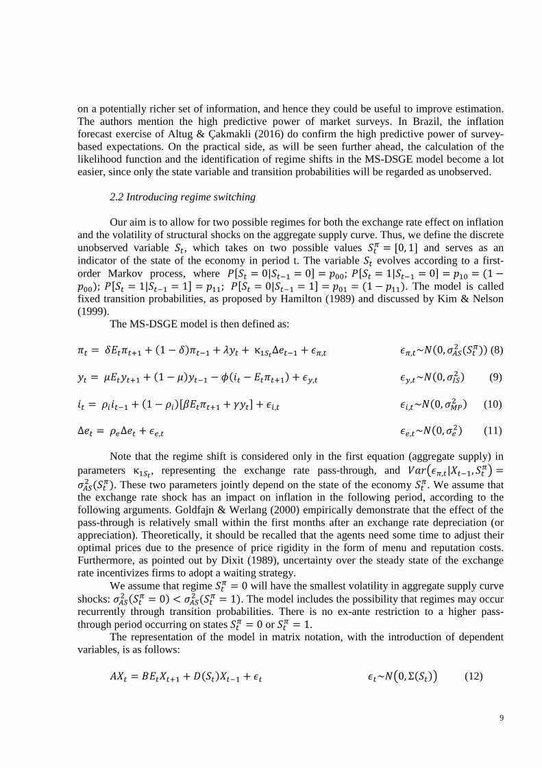
2.2 Introducing regime switching

Our aim is to allow for two possible regimes for both the exchange rate effect on inflation

and the volatility of structural shocks on the aggregate supply curve. Thus, we define the discrete

unobserved variable 𝑆𝑡, which takes on two possible values 𝑆𝑡𝜋 = [0, 1] and serves as an

indicator of the state of the economy in period t. The variable 𝑆𝑡 evolves according to a first-

order Markov process, where 𝑃[𝑆𝑡 = 0|𝑆𝑡−1 = 0] = 𝑝00; 𝑃[𝑆𝑡 = 1|𝑆𝑡−1 = 0] = 𝑝10 = (1 −𝑝00); 𝑃[𝑆𝑡 = 1|𝑆𝑡−1 = 1] = 𝑝11; 𝑃[𝑆𝑡 = 0|𝑆𝑡−1 = 1] = 𝑝01 = (1 − 𝑝11). The model is called

fixed transition probabilities, as proposed by Hamilton (1989) and discussed by Kim & Nelson

(1999). The MS-DSGE model is then defined as:

𝜋𝑡 = 𝛿𝐸𝑡𝜋𝑡+1 + (1 − 𝛿)𝜋𝑡−1 + 𝜆𝑦𝑡 + κ1𝑆𝑡∆𝑒𝑡−1 + 𝜖𝜋,𝑡 𝜖𝜋,𝑡~𝑁(0, 𝜎𝐴𝑆

2 (𝑆𝑡𝜋)) (8)



∆𝑒𝑡 = 𝜌𝑒∆𝑒𝑡 + 𝜖𝑒,𝑡 𝜖𝑒,𝑡~𝑁(0, 𝜎𝑒2) (11)

Note that the regime shift is considered only in the first equation (aggregate supply) in

parameters κ1𝑆𝑡, representing the exchange rate pass-through, and 𝑉𝑎𝑟(𝜖𝜋,𝑡|𝑋𝑡−1, 𝑆𝑡

𝜋) =

𝜎𝐴𝑆2 (𝑆𝑡

𝜋). These two parameters jointly depend on the state of the economy 𝑆𝑡𝜋. We assume that

the exchange rate shock has an impact on inflation in the following period, according to the

following arguments. Goldfajn & Werlang (2000) empirically demonstrate that the effect of the

pass-through is relatively small within the first months after an exchange rate depreciation (or

appreciation). Theoretically, it should be recalled that the agents need some time to adjust their

optimal prices due to the presence of price rigidity in the form of menu and reputation costs.

Furthermore, as pointed out by Dixit (1989), uncertainty over the steady state of the exchange

rate incentivizes firms to adopt a waiting strategy.

We assume that regime 𝑆𝑡𝜋 = 0 will have the smallest volatility in aggregate supply curve

shocks: 𝜎𝐴𝑆2 (𝑆𝑡

𝜋 = 0) < 𝜎𝐴𝑆2 (𝑆𝑡

𝜋 = 1). The model includes the possibility that regimes may occur

recurrently through transition probabilities. There is no ex-ante restriction to a higher pass-

through period occurring on states 𝑆𝑡𝜋 = 0 or 𝑆𝑡

𝜋 = 1.

The representation of the model in matrix notation, with the introduction of dependent

variables, is as follows:

𝐴𝑋𝑡 = 𝐵𝐸𝑡𝑋𝑡+1 + 𝐷(𝑆𝑡)𝑋𝑡−1 + 𝜖𝑡 𝜖𝑡~𝑁(0, Σ(𝑆𝑡)) (12)

10

Where matrix 𝐷(𝑆𝑡) takes on a different value in each regime, and so do the variance-

covariance matrices between structural shocks Σ(𝑆𝑡). Note that the regime shift could also occur

in matrices 𝐴 and 𝐵; however, this will not be necessary in our case. Baele et al. (2015), for

instance, assume regime switching in Taylor rule parameters, which are represented in matrices

𝐴 and 𝐵.

One of the advantages of the representation method adopted by Baele et al. (2015) lies in

its simplicity. Liu & Mumtaz (2010) and Gonçalves, Portugal & Arágon (2016), for example,

follow the state-space representation of the MS-DSGE model to solve the regime-switching

rational expectations model by the extended state vector method proposed by Farmer, Waggoner

& Zha (2011). This yields a state-space MS-VAR model, which uses the algorithm of Kim &

Nelson (1999) for its estimation. Later on, we will describe how the strategy adopted by Baele et

al. (2015) allows solving and assessing the rational expectations equilibrium, in addition to

estimating its parameters in a simpler way.

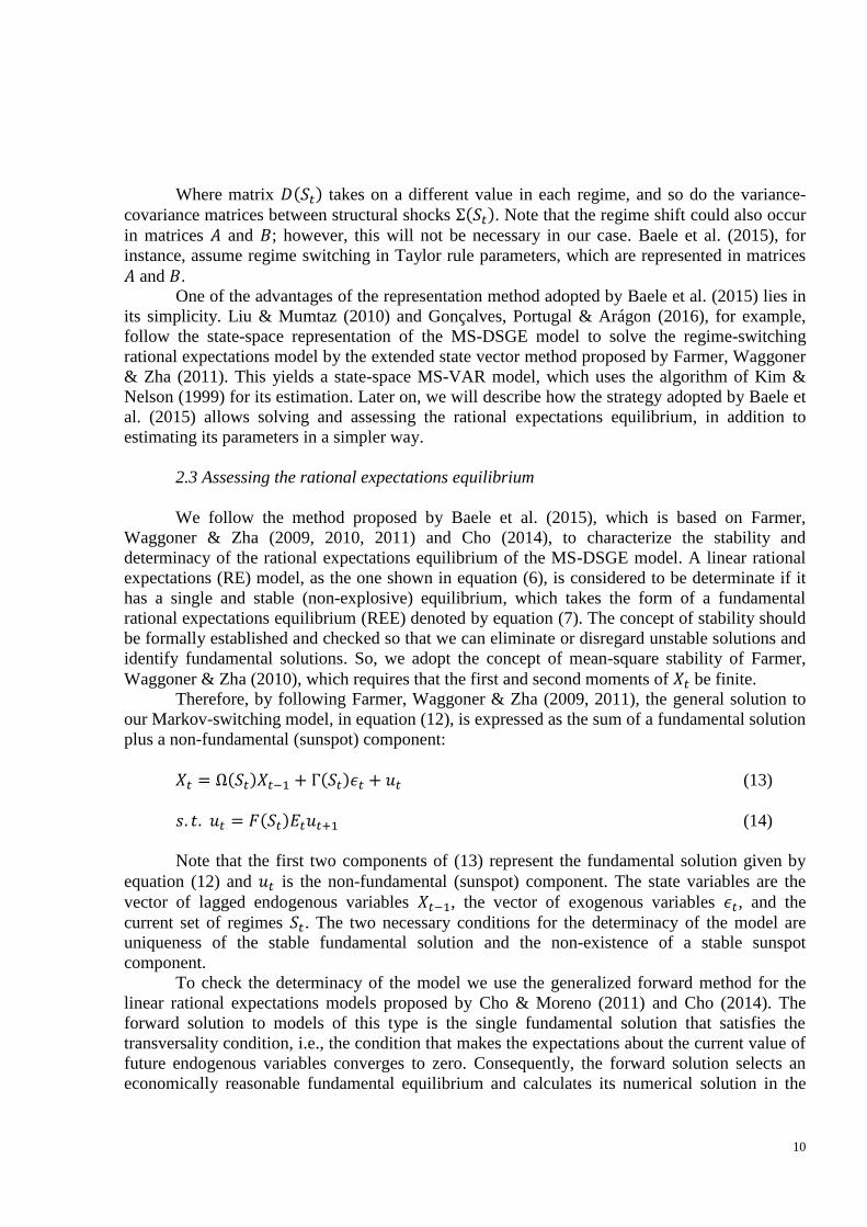
2.3 Assessing the rational expectations equilibrium

We follow the method proposed by Baele et al. (2015), which is based on Farmer,

Waggoner & Zha (2009, 2010, 2011) and Cho (2014), to characterize the stability and

determinacy of the rational expectations equilibrium of the MS-DSGE model. A linear rational

expectations (RE) model, as the one shown in equation (6), is considered to be determinate if it

has a single and stable (non-explosive) equilibrium, which takes the form of a fundamental

rational expectations equilibrium (REE) denoted by equation (7). The concept of stability should

be formally established and checked so that we can eliminate or disregard unstable solutions and

identify fundamental solutions. So, we adopt the concept of mean-square stability of Farmer,

Waggoner & Zha (2010), which requires that the first and second moments of 𝑋𝑡 be finite.

Therefore, by following Farmer, Waggoner & Zha (2009, 2011), the general solution to

our Markov-switching model, in equation (12), is expressed as the sum of a fundamental solution

plus a non-fundamental (sunspot) component:

𝑋𝑡 = Ω(𝑆𝑡)𝑋𝑡−1 + Γ(𝑆𝑡)𝜖𝑡 + 𝑢𝑡 (13)

𝑠. 𝑡. 𝑢𝑡 = 𝐹(𝑆𝑡)𝐸𝑡𝑢𝑡+1 (14)

Note that the first two components of (13) represent the fundamental solution given by

equation (12) and 𝑢𝑡 is the non-fundamental (sunspot) component. The state variables are the

vector of lagged endogenous variables 𝑋𝑡−1, the vector of exogenous variables 𝜖𝑡, and the

current set of regimes 𝑆𝑡. The two necessary conditions for the determinacy of the model are

uniqueness of the stable fundamental solution and the non-existence of a stable sunspot

component.

To check the determinacy of the model we use the generalized forward method for the

linear rational expectations models proposed by Cho & Moreno (2011) and Cho (2014). The

forward solution to models of this type is the single fundamental solution that satisfies the

transversality condition, i.e., the condition that makes the expectations about the current value of

future endogenous variables converges to zero. Consequently, the forward solution selects an

economically reasonable fundamental equilibrium and calculates its numerical solution in the

11

same step. Cho (2014) demonstrates that the rationale behind the forward solution also applies to

Markov-switching models, providing easily treatable formal conditions using the mean-square

stability concept.

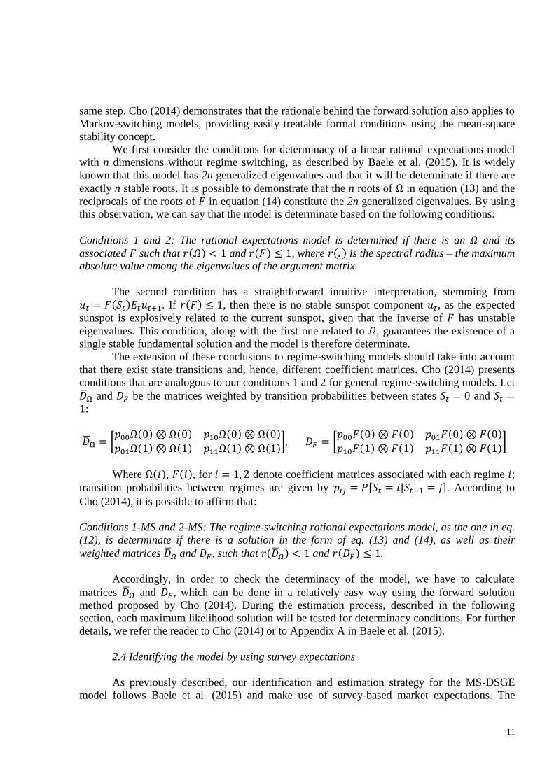
We first consider the conditions for determinacy of a linear rational expectations model

with n dimensions without regime switching, as described by Baele et al. (2015). It is widely

known that this model has 2n generalized eigenvalues and that it will be determinate if there are

exactly n stable roots. It is possible to demonstrate that the n roots of Ω in equation (13) and the

reciprocals of the roots of 𝐹 in equation (14) constitute the 2n generalized eigenvalues. By using

this observation, we can say that the model is determinate based on the following conditions:

Conditions 1 and 2: The rational expectations model is determined if there is an 𝛺 and its

associated 𝐹 such that 𝑟(𝛺) < 1 and 𝑟(𝐹) ≤ 1, where 𝑟(. ) is the spectral radius – the maximum

absolute value among the eigenvalues of the argument matrix.

The second condition has a straightforward intuitive interpretation, stemming from

𝑢𝑡 = 𝐹(𝑆𝑡)𝐸𝑡𝑢𝑡+1. If 𝑟(𝐹) ≤ 1, then there is no stable sunspot component 𝑢𝑡, as the expected

sunspot is explosively related to the current sunspot, given that the inverse of 𝐹 has unstable

eigenvalues. This condition, along with the first one related to 𝛺, guarantees the existence of a

single stable fundamental solution and the model is therefore determinate.

The extension of these conclusions to regime-switching models should take into account

that there exist state transitions and, hence, different coefficient matrices. Cho (2014) presents

conditions that are analogous to our conditions 1 and 2 for general regime-switching models. Let

�̅�Ω and 𝐷𝐹 be the matrices weighted by transition probabilities between states 𝑆𝑡 = 0 and 𝑆𝑡 =1:

�̅�Ω = [𝑝00Ω(0) ⊗ Ω(0) 𝑝10Ω(0) ⊗ Ω(0)

𝑝01Ω(1) ⊗ Ω(1) 𝑝11Ω(1) ⊗ Ω(1)], 𝐷𝐹 = [

𝑝00𝐹(0) ⊗ 𝐹(0) 𝑝01𝐹(0) ⊗ 𝐹(0)

𝑝10𝐹(1) ⊗ 𝐹(1) 𝑝11𝐹(1) ⊗ 𝐹(1)]

Where Ω(𝑖), 𝐹(𝑖), for 𝑖 = 1, 2 denote coefficient matrices associated with each regime 𝑖; transition probabilities between regimes are given by 𝑝𝑖𝑗 = 𝑃[𝑆𝑡 = 𝑖|𝑆𝑡−1 = 𝑗]. According to

Cho (2014), it is possible to affirm that:

Conditions 1-MS and 2-MS: The regime-switching rational expectations model, as the one in eq.

(12), is determinate if there is a solution in the form of eq. (13) and (14), as well as their

weighted matrices �̅�𝛺 and 𝐷𝐹, such that 𝑟(�̅�𝛺) < 1 and 𝑟(𝐷𝐹) ≤ 1.

Accordingly, in order to check the determinacy of the model, we have to calculate

matrices �̅�Ω and 𝐷𝐹, which can be done in a relatively easy way using the forward solution

method proposed by Cho (2014). During the estimation process, described in the following

section, each maximum likelihood solution will be tested for determinacy conditions. For further

details, we refer the reader to Cho (2014) or to Appendix A in Baele et al. (2015).

2.4 Identifying the model by using survey expectations

As previously described, our identification and estimation strategy for the MS-DSGE

model follows Baele et al. (2015) and make use of survey-based market expectations. The

12

authors assume that market expectations for inflation and for output gap follow the law of

motion below:

𝜋𝑡𝑓

= 𝛼𝐸𝑡𝜋𝑡+1 + (1 − 𝛼)𝜋𝑡−1𝑓

+ 𝑤𝑡𝜋 𝑤𝑡

𝜋~𝑁(0, 𝜎𝑓𝜋) (15)

𝑦𝑡𝑓

= 𝛼𝐸𝑡𝑦𝑡+1 + (1 − 𝛼)𝑦𝑡−1𝑓

+ 𝑤𝑡𝑦

𝑤𝑡𝑦~𝑁(0, 𝜎𝑓

𝑦) (16)

These two equations allow for a slow adjustment mechanism in expectations formation,

in which survey expectations potentially react to rational expectations one to one only when

parameter 𝛼 is equal to 1. Otherwise, the adjustment of expectations is slower and depends on

past values. The process is inspired in Mankiw & Reis’s (2002) model of the Phillips curve in

which the information disseminates slowly.

Baele et al. (2015) simplify the estimation mechanism by assuming that the volatility of

shocks 𝜎𝑓𝜋 and 𝜎𝑓

𝑦 in the equations for expectations movement is equal to zero. In this case, the

survey-based expectations are the exact function of current rational expectations and of the past

values from the survey. Substituting both equations above into our main model, we have:

𝜋𝑡 = 𝛿

𝛼(𝜋𝑡

𝑓− (1 − 𝛼)𝜋𝑡−1

𝑓) + (1 − 𝛿)𝜋𝑡−1 + 𝜆𝑦𝑡 + κ1𝑆𝑡

∆𝑒𝑡−1 + 𝜖𝜋,𝑡 (17)

𝑦𝑡 = 𝜇

𝛼(𝑦𝑡

𝑓− (1 − 𝛼)𝑦𝑡−1

𝑓) + (1 − 𝜇)𝑦𝑡−1 − 𝜙𝑖𝑡 +

𝜙

𝛼(𝜋𝑡

𝑓− (1 − 𝛼)𝜋𝑡−1

𝑓) + 𝜖𝑦,𝑡 (18)

𝑖𝑡 = 𝜌𝑖𝑖𝑡−1 + (1 − 𝜌𝑖) [𝛽

𝛼(𝜋𝑡

𝑓− (1 − 𝛼)𝜋𝑡−1

𝑓) + 𝛾𝑦𝑡] + 𝜖𝑖,𝑡 (19)

∆𝑒𝑡 = 𝜌𝑒∆𝑒𝑡 + 𝜖𝑒,𝑡 (20)

Where 𝜖𝜋,𝑡~𝑁(0, 𝜎𝐴𝑆2 (𝑆𝑡)), 𝜖𝑦,𝑡~𝑁(0, 𝜎𝐼𝑆

2 ), 𝜖𝑖,𝑡~𝑁(0, 𝜎𝑀𝑃2 ), 𝜖𝑒,𝑡~𝑁(0, 𝜎𝑒

2). Note that

when 𝛼 = 1, it is assumed that the rational expectations are equivalent to the survey

expectations. Defining 𝑋𝑡𝑓

= [𝜋𝑡𝑓 𝑦𝑡

𝑓]′, we can write the model in matrix form:

𝐴𝑋𝑡 = 𝐵𝑋𝑡𝑓+ 𝐷𝑋𝑡−1

𝑓+ 𝐺𝑆𝑡

𝑋𝑡−1 + 𝜖𝑡 𝜖𝑡~𝑁(0, Σ(𝑆𝑡)) (21)

Where the matrices are specified as follows:

𝐴 = [

1 −𝜆 0 00 1 𝜙 0

0 −(1 − 𝜌𝑖)𝛾 1 00 0 0 1

]

𝐺𝑆𝑡=

[ (1 − 𝛿) 0 0 κ1𝑆𝑡

0 (1 − 𝜇) 0 00 0 𝜌𝑖 00 0 0 𝜌𝑒 ]

13

𝐵 =

[

𝛿

𝛼0

𝜙

𝛼

𝜇

𝛼(1 − 𝜌𝑖)𝛽

𝛼0

0 0]

𝐷 =

[ −

𝛿(1 − 𝛼)

𝛼0

−𝜙(1 − 𝛼)

𝛼

−𝜇(1 − 𝛼)

𝛼−(1 − 𝜌𝑖)(1 − 𝛼)𝛽

𝛼0

0 0 ]

Σ(𝑆𝑡) =

[ 𝜎𝐴𝑆

2 (𝑆𝑡) 0 0 0

0 𝜎𝐼𝑆2 0 0

0 0 𝜎𝑀𝑃2 0

0 0 0 𝜎𝑒2]

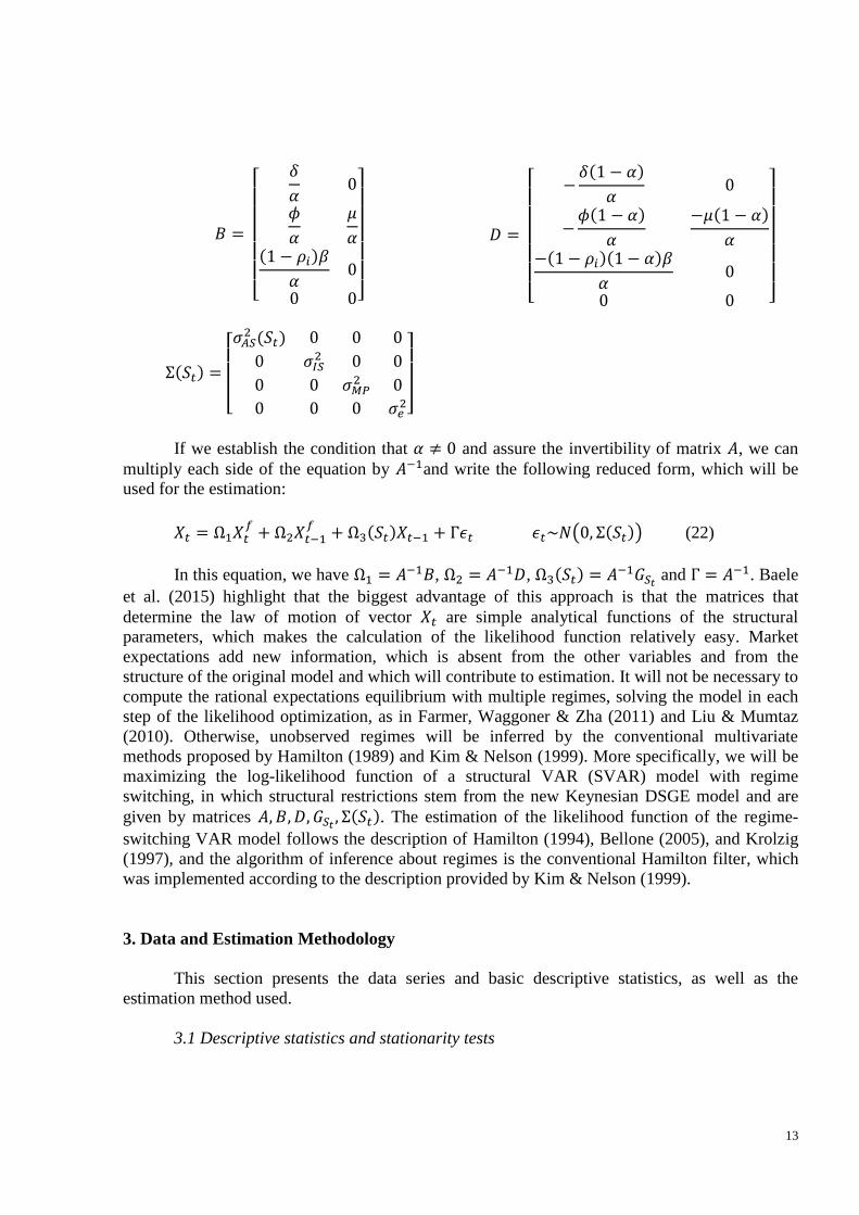
If we establish the condition that 𝛼 ≠ 0 and assure the invertibility of matrix 𝐴, we can

multiply each side of the equation by 𝐴−1and write the following reduced form, which will be

used for the estimation:

𝑋𝑡 = Ω1𝑋𝑡𝑓

+ Ω2𝑋𝑡−1𝑓

+ Ω3(𝑆𝑡)𝑋𝑡−1 + Γ𝜖𝑡 𝜖𝑡~𝑁(0, Σ(𝑆𝑡)) (22)

In this equation, we have Ω1 = 𝐴−1𝐵, Ω2 = 𝐴−1𝐷, Ω3(𝑆𝑡) = 𝐴−1𝐺𝑆𝑡 and Γ = 𝐴−1. Baele

et al. (2015) highlight that the biggest advantage of this approach is that the matrices that

determine the law of motion of vector 𝑋𝑡 are simple analytical functions of the structural

parameters, which makes the calculation of the likelihood function relatively easy. Market

expectations add new information, which is absent from the other variables and from the

structure of the original model and which will contribute to estimation. It will not be necessary to

compute the rational expectations equilibrium with multiple regimes, solving the model in each

step of the likelihood optimization, as in Farmer, Waggoner & Zha (2011) and Liu & Mumtaz

(2010). Otherwise, unobserved regimes will be inferred by the conventional multivariate

methods proposed by Hamilton (1989) and Kim & Nelson (1999). More specifically, we will be

maximizing the log-likelihood function of a structural VAR (SVAR) model with regime

switching, in which structural restrictions stem from the new Keynesian DSGE model and are

given by matrices 𝐴, 𝐵, 𝐷, 𝐺𝑆𝑡, Σ(𝑆𝑡). The estimation of the likelihood function of the regime-

switching VAR model follows the description of Hamilton (1994), Bellone (2005), and Krolzig

(1997), and the algorithm of inference about regimes is the conventional Hamilton filter, which

was implemented according to the description provided by Kim & Nelson (1999).

3. Data and Estimation Methodology

This section presents the data series and basic descriptive statistics, as well as the

estimation method used.

3.1 Descriptive statistics and stationarity tests

14

The estimation of the model requires six observed variables: inflation, output gap, interest

rate, exchange rate movement, and the survey expectations for inflation and output gap. Sixty-

four quarterly observations – from the first quarter of 2000 to the fourth quarter of 2015 – were

considered for the sample. We opted to leave the year 1999 out of the sample due to the large

fluctuations observed shortly after the transition to the floating exchange rate regime, and also

because data on survey expectations are not readily available.

The seasonally adjusted quarterly IPCA (%), Indice de Precos ao Consumidor Amplo,

was used for consumer price inflation. First, the monthly series2 was accumulated quarterly and

then we applied a multiplicative moving average seasonal adjustment. The output gap was

obtained from the quarterly GDP logarithm at seasonally adjusted market values3 and the trend

was estimated by the Hodrick-Prescott (HP) filter. The remaining component (business cycle)

was considered to be the output gap. A broader window, beginning in 1996, was used for

extracting the gap so as to avoid the tail effect at the beginning of the period. In turn, the

quarterly exchange rate movement is calculated as the first difference of the nominal exchange

rate value, BRL (Brazilian Reais) vis-à-vis USD (United States Dollars), at the end of the

period.4

We choose to use as the quarterly interest rate it the nominal interest rate discounted for

the long-run real interest rate. In this sense, we try to account for the fact that the Brazilian

economy experienced a sharp reduction in its long-run real interest rate between 2005 and 2012.

Thus, the data we are taking to the model is the nominal rate in excess of the long run interest

rate, and we should obviously consider this characteristic when analysing our estimation results.

In order to calculate our series it, we first took the quarterly equivalent of the monthly Selic Over

rate (% p.a.)5 at end of the period. The long-run real interest rate was built from the trend of an

HP filter under the real interest rate, which is determined by the nominal rate minus the observed

inflation. We then discount the long-run real interest rate from our quarterly nominal interest

rate.

Finally, the Central Bank of Brazil’s6 survey-based market expectations were used to

calculate inflation and output gap expectations for the subsequent quarter. Inflation expectation

was measured as the median value of the survey for the consumer prices inflation (IPCA) for the

three months of the subsequent quarter, observed on the first business day of the current quarter.

The monthly values were accumulated to obtain the quarterly inflation expectation. Data

observed on the first business day is used to circumvent the endogeneity problem between

inflation in the current quarter and inflation expectations for the subsequent period, without

having to rely on instrumental variables. In fact, one avoids the correlation between exogenous

shock to inflation in the current period 𝜖𝜋,𝑡 and future expectations 𝐸𝑡𝜋𝑡+1 as basically

information from the current period is not included in the measure.

On the other hand, it was necessary to use a calculation procedure to obtain the output

gap expectations for the subsequent quarter. The variable observed by the market survey is the

real growth of GDP (% per year) for the subsequent quarter. The first step consisted in extracting

the equivalent quarterly growth rate, and then estimating the real domestic product expected for

t+1. The seasonally adjusted series observed in the past was included up to period t, under the

2 Source: Series 433 (monthly IPCA). Central Bank of Brazil Time Series.

3 Source: Series 22109 (seasonally adjusted GDP). Central Bank of Brazil Time Series.

4 Source: Series 3696 (free exchange rate). Central Bank of Brazil Time Series.

5 Source: Monthly Over/Selic interest rate (% p.a.) series. IPEA Data System.

6 Source: Central Bank of Brazil Market Expectations System (Focus Report).

15

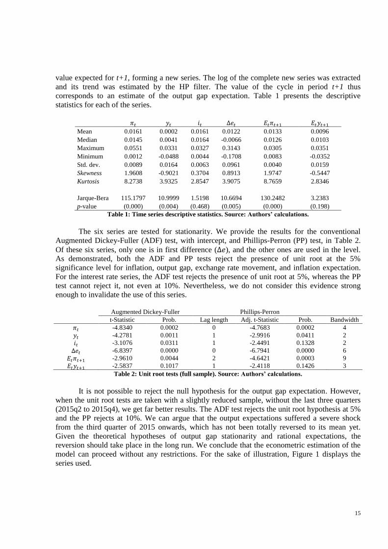
value expected for t+1, forming a new series. The log of the complete new series was extracted

and its trend was estimated by the HP filter. The value of the cycle in period t+1 thus

corresponds to an estimate of the output gap expectation. Table 1 presents the descriptive

statistics for each of the series.

𝜋𝑡 𝑦𝑡 𝑖𝑡 ∆𝑒𝑡 𝐸𝑡𝜋𝑡+1 𝐸𝑡𝑦𝑡+1

Mean 0.0161 0.0002 0.0161 0.0122 0.0133 0.0096

Median 0.0145 0.0041 0.0164 -0.0066 0.0126 0.0103

Maximum 0.0551 0.0331 0.0327 0.3143 0.0305 0.0351

Minimum 0.0012 -0.0488 0.0044 -0.1708 0.0083 -0.0352

Std. dev. 0.0089 0.0164 0.0063 0.0961 0.0040 0.0159

Skewness 1.9608 -0.9021 0.3704 0.8913 1.9747 -0.5447

Kurtosis 8.2738 3.9325 2.8547 3.9075 8.7659 2.8346

Jarque-Bera 115.1797 10.9999 1.5198 10.6694 130.2482 3.2383

p-value (0.000) (0.004) (0.468) (0.005) (0.000) (0.198)

Table 1: Time series descriptive statistics. Source: Authors’ calculations.

The six series are tested for stationarity. We provide the results for the conventional

Augmented Dickey-Fuller (ADF) test, with intercept, and Phillips-Perron (PP) test, in Table 2.

Of these six series, only one is in first difference (∆𝑒), and the other ones are used in the level.

As demonstrated, both the ADF and PP tests reject the presence of unit root at the 5%

significance level for inflation, output gap, exchange rate movement, and inflation expectation.

For the interest rate series, the ADF test rejects the presence of unit root at 5%, whereas the PP

test cannot reject it, not even at 10%. Nevertheless, we do not consider this evidence strong

enough to invalidate the use of this series.

Augmented Dickey-Fuller Phillips-Perron

t-Statistic Prob. Lag length Adj. t-Statistic Prob. Bandwidth

𝜋𝑡 -4.8340 0.0002 0 -4.7683 0.0002 4

𝑦𝑡 -4.2781 0.0011 1 -2.9916 0.0411 2

𝑖𝑡 -3.1076 0.0311 1 -2.4491 0.1328 2

∆𝑒𝑡 -6.8397 0.0000 0 -6.7941 0.0000 6

𝐸𝑡𝜋𝑡+1 -2.9610 0.0044 2 -4.6421 0.0003 9

𝐸𝑡𝑦𝑡+1 -2.5837 0.1017 1 -2.4118 0.1426 3

Table 2: Unit root tests (full sample). Source: Authors’ calculations.

It is not possible to reject the null hypothesis for the output gap expectation. However,

when the unit root tests are taken with a slightly reduced sample, without the last three quarters

(2015q2 to 2015q4), we get far better results. The ADF test rejects the unit root hypothesis at 5%

and the PP rejects at 10%. We can argue that the output expectations suffered a severe shock

from the third quarter of 2015 onwards, which has not been totally reversed to its mean yet.

Given the theoretical hypotheses of output gap stationarity and rational expectations, the

reversion should take place in the long run. We conclude that the econometric estimation of the

model can proceed without any restrictions. For the sake of illustration, Figure 1 displays the

series used.

16

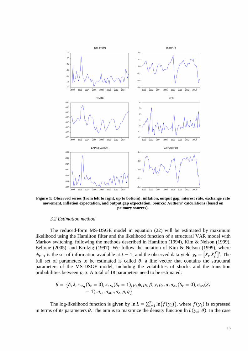
Figure 1: Observed series (from left to right, up to bottom): inflation, output gap, interest rate, exchange rate

movement, inflation expectation, and output gap expectation. Source: Authors’ calculations (based on

primary sources).

3.2 Estimation method

The reduced-form MS-DSGE model in equation (22) will be estimated by maximum

likelihood using the Hamilton filter and the likelihood function of a structural VAR model with

Markov switching, following the methods described in Hamilton (1994), Kim & Nelson (1999),

Bellone (2005), and Krolzig (1997). We follow the notation of Kim & Nelson (1999), where

𝜓𝑡−1 is the set of information available at 𝑡 − 1, and the observed data yield 𝑦𝑡 = [𝑋𝑡 𝑋𝑡𝑓]′. The

full set of parameters to be estimated is called 𝜃, a line vector that contains the structural

parameters of the MS-DSGE model, including the volatilities of shocks and the transition

probabilities between 𝑝, 𝑞. A total of 18 parameters need to be estimated:

𝜃 = {𝛿, 𝜆, 𝜅1𝑆𝑡(𝑆𝑡 = 0), 𝜅1𝑆𝑡

(𝑆𝑡 = 1), 𝜇, 𝜙, 𝜌𝑖 , 𝛽, 𝛾, 𝜌𝑒 , 𝛼, 𝜎𝐴𝑆(𝑆𝑡 = 0), 𝜎𝐴𝑆(𝑆𝑡

= 1), 𝜎𝐼𝑆, 𝜎𝑀𝑃, 𝜎𝑒 , 𝑝, 𝑞}

The log-likelihood function is given by ln 𝐿 = ∑ ln (𝑓(𝑦𝑡))𝑇𝑡=1 , where 𝑓(𝑦𝑡) is expressed

in terms of its parameters 𝜃. The aim is to maximize the density function ln 𝐿(𝑦𝑡; 𝜃). In the case

.00

.01

.02

.03

.04

.05

.06

2000 2002 2004 2006 2008 2010 2012 2014

INFLATION

-.06

-.04

-.02

.00

.02

.04

2000 2002 2004 2006 2008 2010 2012 2014

OUTPUT

.000

.005

.010

.015

.020

.025

.030

.035

2000 2002 2004 2006 2008 2010 2012 2014

RRATE

-.2

-.1

.0

.1

.2

.3

.4

2000 2002 2004 2006 2008 2010 2012 2014

DFX

.008

.012

.016

.020

.024

.028

.032

2000 2002 2004 2006 2008 2010 2012 2014

EXPINFLATION

-.04

-.02

.00

.02

.04

2000 2002 2004 2006 2008 2010 2012 2014

EXPOUTPUT

17

of regime-switching models, we do not observe regimes 𝑆𝑡, but we can infer about them in every

time period. Kim & Nelson (1999) describe the following steps to determine the log-likelihood

function of a general regime-switching model.

Step 1: First, one should consider the joint density of 𝑦𝑡 and the unobserved variable 𝑆𝑡, based on

the information up to 𝑡 − 1, which is given by the product of conditional and marginal density:

𝑓(𝑦𝑡, 𝑆𝑡|𝜓𝑡−1) = 𝑓(𝑦𝑡|𝑆𝑡, 𝜓𝑡−1)𝑓(𝑆𝑡| 𝜓𝑡−1)

Step 2: Then, in order to obtain the marginal density of 𝑦𝑡, the variable 𝑆𝑡 is included in the joint

density by the sum of all the possible values for 𝑆𝑡:

𝑓(𝑦𝑡|𝜓𝑡−1) = ∑ 𝑓(𝑦𝑡, 𝑆𝑡| 𝜓𝑡−1)

1

𝑆𝑡=0

= ∑ 𝑓(𝑦𝑡|𝑆𝑡, 𝜓𝑡−1)𝑓(𝑆𝑡| 𝜓𝑡−1)

1

𝑆𝑡=0

In the case of only two regimes, we have 𝑓(𝑆𝑡 = 𝑗| 𝜓𝑡−1) = 𝑃𝑟[𝑆𝑡 = 𝑗| 𝜓𝑡−1], and the

log-likelihood function is given by:

ln 𝐿 = ∑ ln{∑ 𝑓(𝑦𝑡|𝑆𝑡, 𝜓𝑡−1)1𝑆𝑡=0 𝑃𝑟[𝑆𝑡| 𝜓𝑡−1]}

𝑇𝑡=1 (23)

Kim & Nelson (1999) underscore that the marginal density above can be interpreted as a

weighted average between conditional densities, in the cases where 𝑆𝑡 = 0 and 𝑆𝑡 = 1. To derive

the marginal density and also the log-likelihood, it is necessary to calculate the weighting factors

𝑃𝑟[𝑆𝑡 = 0| 𝜓𝑡−1] and 𝑃𝑟[𝑆𝑡 = 1| 𝜓𝑡−1]. At this moment, we assume that the discrete variable 𝑆𝑡

follows a first-order Markov process, where its state at 𝑡 depends only on its previous state 𝑆𝑡−1.

We again follow Kim & Nelson (1999) to define the transition probabilities 𝑝 and 𝑞: 𝑝 = 𝑃𝑟[𝑆𝑡 = 1|𝑆𝑡−1 = 1], and 𝑞 = 𝑃𝑟[𝑆𝑡 = 0|𝑆𝑡−1 = 0].

In the case of the Markov process, we use a filter to calculate the weighting factors

𝑃𝑟[𝑆𝑡 = 𝑗| 𝜓𝑡−1], 𝑗 = 0, 1, which takes into account the transition probabilities between states:

Step 1: Given 𝑃𝑟[𝑆𝑡−1 = 𝑖| 𝜓𝑡−1], for 𝑖 = 0, 1, at the beginning of period 𝑡, the weighting term

is calculated as

𝑃𝑟[𝑆𝑡 = 𝑗| 𝜓𝑡−1] = ∑ 𝑃𝑟[𝑆𝑡 = 𝑗, 𝑆𝑡−1 = 𝑖| 𝜓𝑡−1]1

𝑖=0= ∑ 𝑃𝑟[𝑆𝑡 = 𝑗|𝑆𝑡−1 = 𝑖]𝑃𝑟[𝑆𝑡−1 = 𝑖| 𝜓𝑡−1]

1

𝑖=0

Where 𝑃𝑟[𝑆𝑡 = 𝑗|𝑆𝑡−1 = 𝑖] are the transition probabilities between states.

Step 2: Once 𝑦𝑡, is observed at the end of period 𝑡, we can update the probability term as follows

𝑃𝑟[𝑆𝑡 = 𝑗| 𝜓𝑡] = 𝑃𝑟[𝑆𝑡 = 𝑗| 𝜓𝑡−1, 𝑦𝑡] =𝑓(𝑆𝑡 = 𝑗, 𝑦𝑡|𝜓𝑡−1)

𝑓(𝑦𝑡|𝜓𝑡−1)

=𝑓(𝑦𝑡|𝑆𝑡 = 𝑗, 𝜓𝑡−1)𝑃𝑟[𝑆𝑡 = 𝑗| 𝜓𝑡−1]

∑ 𝑓(𝑦𝑡|𝑆𝑡 = 𝑗, 𝜓𝑡−1)1𝑗=0 𝑃𝑟[𝑆𝑡 = 𝑗| 𝜓𝑡−1]

18

Where 𝜓𝑡 = { 𝜓𝑡−1, 𝑦𝑡}. The steps above are performed iteratively to calculate 𝑃𝑟[𝑆𝑡 =𝑗| 𝜓𝑡], 𝑡 = 1,2, … , 𝑇, i.e., the filtered probabilities for the whole sampling period. To initiate the

filter at 𝑡 = 1, we assume unconditional probabilities, or steady state, at 𝑡 = 0:

𝑃𝑟[𝑆0 = 0| 𝜓0] =1 − 𝑝

2 − 𝑝 − 𝑞 𝑃𝑟[𝑆0 = 1| 𝜓0] =

1 − 𝑞

2 − 𝑝 − 𝑞

The description of the steps above and of the probability update filter makes it clear that

the marginal density 𝑓(𝑦𝑡|𝜓𝑡−1) is a function of parameters 𝜃, which include the traditional

likelihood parameters, the parameters that vary across states, in addition to the transition

probabilities for state 𝑝, 𝑞. In the case of the Markov-switching model, the log-likelihood

function of equation (23) is then given by:

ln 𝐿 = ∑ ln{∑ 𝑓(𝑦𝑡|𝑆𝑡, 𝜓𝑡−1)1𝑆𝑡=0 𝑃𝑟[𝑆𝑡| 𝜓𝑡−1]}

𝑇𝑡=1 (24)

In what follows, we describe some peculiarities about the algorithm implemented for our

estimation.7 We begin by assigning an initial value to each parameter of vector 𝜃0. The initial

values were chosen based on estimation results obtained by Baele et al. (2015) and are displayed

in Table 3.

From the value of 𝜃0, we maximize the log-likelihood function with a numerical

constraint optimization algorithm. In each optimization step, the parameters of the candidate

vector 𝜃𝑖 are used for the construction of matrices 𝐴, 𝐵, 𝐷, 𝐺𝑆𝑡, Σ(𝑆𝑡), which represent the model

in its structural form. We proceeded directly with the computation of matrices Ω1, Ω2,Ω3(𝑆𝑡), Γ to

change the model into its reduced form. With the matrices in reduced form and transition

probabilities, the log-likelihood calculation was then made using the Hamilton filter, described

previously, and the sample likelihood function of an MS-VAR model, shown next

(HAMILTON, 1994; BELLONE, 2005; KROLZIG, 1997). At last, we check whether the

determinacy conditions for the rational expectations equilibrium are met with each candidate

solution vector 𝜃𝑖, and we penalize the objective function if that is not the case. This procedure

will guarantee that the search will be made along a stable solution path.

Let 𝑛 = 4 be the number of endogenous variables, 𝑚 = 8 the number of regressors of

the reduced model, and 𝑇 = 64 the number of observations. Following Hamilton’s (1994)

notation, consider:

𝑦𝑡 = [𝑋𝑡] the vector of endogenous variables, 𝑛𝑥1;

𝑥𝑡 = [𝑋𝑡𝑓 𝑋𝑡−1

𝑓 𝑋𝑡−1] the vector containing the grouped regressors of the reduced model,

𝑚𝑥1;

Ω𝑉𝑎𝑟(𝑆𝑡) = Γ Σ(𝑆𝑡)Γ′ the variance-covariance matrix of the reduced model for each state

obtained from Σ(𝑆𝑡) and from Γ, 𝑛𝑥𝑛;

Π(𝑆𝑡)′ = [Ω1 Ω2 Ω3(𝑆𝑡)] the state-dependent coefficient matrix of the reduced model, 𝑛𝑥𝑚.

The same reduced model in equation (22) can be written as a regime-switching VAR

model:

𝑦𝑡 = Π(𝑆𝑡)′𝑥𝑡 + 𝑢𝑡 𝑢𝑡~𝑁(0, Ω𝑉𝑎𝑟(𝑆𝑡)) (25)

7 The estimation algorithm was implemented using Matlab R2011 and is available upon request.

19

After defining this notation for each filtering step, the marginal density of the VAR

model, given 𝜃, 𝑆𝑡, 𝜓𝑡−1, is as follows:

𝑓(𝑦𝑡|𝜃, 𝑆𝑡 , 𝜓𝑡−1) = (2𝜋)−𝑛/2√|(Ω𝑉𝑎𝑟(𝑆𝑡))−1

| exp {−1

2[𝑦𝑡 − (Π(𝑆𝑡)

′𝑥𝑡)]′(Ω𝑉𝑎𝑟(𝑆𝑡))−1

[𝑦𝑡 − (Π(𝑆𝑡)′𝑥𝑡)]}

The log-likelihood maximization yields a vector of optimal estimated parameters 𝜃.

Parameter Initial value Minimum Maximum

𝛿 0.425 0.00001 1

𝜆 0.102 0.00001 +∞

𝜅1𝑆𝑡(𝑆𝑡 = 0) 0.005 −∞ +∞

𝜅1𝑆𝑡(𝑆𝑡 = 1) 0.09 −∞ +∞

𝜇 0.675 0.00001 1

𝜙 0.10 0.00001 +∞

𝜌𝑖 0.834 0.00001 0.99999

𝛽 1.10 0.00001 +∞

𝛾 0.80 0.00001 +∞

𝜌𝑒 0.16 −∞ 0.99999

𝛼 0.90 0.00001 1

𝜎𝐴𝑆(𝑆𝑡 = 0) 0.0038 0.00001 +∞

𝜎𝐴𝑆(𝑆𝑡 = 1) 0.0098 0.00001 +∞

𝜎𝐼𝑆 0.0108 0.00001 +∞

𝜎𝑀𝑃 0.0043 0.00001 +∞

𝜎𝑒 0.0950 0.00001 +∞

𝑝 0.90 0 1

𝑞 0.76 0 1

Table 3: Initial parameters and restrictions of the MS-DSGE model. Source: Authors’ calculations.

It should be underscored that the parameters are restricted to a domain of possible values,

which are also shown in Table 3, and which stem from the theoretical constraints of the original

DSGE model. Our constraints are similar, but lighter than those of Baele et al. (2015). The

referenced authors initially allow the parameters to be free, but latter present a set of values for

each parameter (domain), calculated by grid search, for which the solution to the model is more

likely. We opted to implement a simpler process by applying some basic theoretical constraints

directly to the initial parameter domain, which will be used in the numerical constrained

optimization. Note that the estimated vector 𝜃 was calculated by verifying the determinacy

conditions for rational expectations solution at each step of the optimization in both cases.

4. Empirical results

In this section, we first discuss the estimation results for the MS-DSGE model, which

allows for joint Markov switching in the exchange rate pass-through coefficient and in the

volatility of shocks to inflation, and then we compare them with the results obtained for the

conventional fixed coefficients model. In what follows, we introduce some specification and

20

linearity tests and we analyze the impulse response functions. Finally, we describe the regimes

identified by the MS-DSGE model and their relationship with economic periods.

4.1 Parameter estimation in the MS-DSGE model

Table 4 shows the estimates for each parameter in the MS-DSGE model, as well as their

standard deviation and corresponding p-value obtained in the conventional t test. The variance-

covariance matrix of the maximum likelihood estimates was calculated using the information

matrix outer product method, as suggested by Hamilton (1994). The solution offered by the

model characterizes a fundamental stable rational expectations equilibrium, as shown in detail in

Section 2.3. The determinacy conditions for the regime-switching rational expectations model

were assessed and confirmed: 𝑟(�̅�𝛺) < 1 and 𝑟(𝐷𝐹) ≤ 1.

Most parameters are statistically significant. Recall that the signs of the parameters are

guaranteed by the constraints imposed on the likelihood function optimization and that no

parameter was calibrated. The parameters for which joint regime switching was allowed were the

pass-through coefficient 𝜅1𝑆𝑡 and the volatility of shocks 𝜎𝐴𝑆(𝑆𝑡

𝜋) to inflation.

In the aggregate supply (AS) equation of the MS-DSGE model we estimated 𝛿 =0.6971, demonstrating a relatively heavier weight to inflation expectations in comparison to the

endogenous persistence (backward-looking) term. This value is quite close to the estimates made

by Silveira (2008), who found 𝛿 = 0.61 in his model with price indexation. In the demand curve

(IS), however, a lighter weight was attached to the expectations element, with 𝜇 = 0.1234, and a

higher standard deviation. This finding suggests, on the one hand, higher output persistence and,

on the other hand, smaller predictive power of market expectations about output performance in

the subsequent periods perhaps as a result of the high volatility of shocks to demand (𝜎𝐼𝑆).

Silveira (2008), in his model with habit formation in consumption, found parameters that would

correspond to 𝜇 = 0.26, and a confidence interval that would include our value of 𝜇 = 0.12. By

and large, we may assume that the model provides evidence in favor of endogenous persistence

of both output and inflation.

The response of inflation to the output gap is estimated at the value of 𝜆 = 0.0722, which

is in line with Bayesian estimations of more complex DSGE models such as Gonçalves, Portugal

& Arágon (2016) who yielded 𝜆 = 0.0654. Our result, however, does not display statistical

significance due to a relatively high standard deviation. Actually, several studies on the Phillips

curve for the Brazilian economy do not demonstrate a statistically significant impact of the

output gap, or of marginal cost, on inflation (Alves & Areosa, 2005; Areosa & Medeiros, 2007;

Arruda, Ferreira & Castelar, 2008), prompting Sachsida (2013) to put the validity of this

assumption into question. An exception is seen in Mazali & Divino (2010), who estimate the

new Keynesian curve with General Method of Moments (GMM), controlling for the exchange

rate pass-through and observe a significant effect of unemployment on inflation. Estimations that

use other series to represent the output gap, such as the Beveridge-Nelson decomposition

suggested by Tristão & Torrent (2015), were tested; however, none of them provided a better fit

than the one introduced herein. Anyway, further investigation into this topic is not within the

scope of this paper.

The MS-DSGE model identifies two distinct regimes regarding the behavior of the

exchange rate pass-through, confirming the major assumption of our paper. We refer to the

regimes as 𝑆𝑡 = 0 and 𝑆𝑡 = 1, which correspond to low and high exchange rate pass-through

periods, respectively. The value estimated in the AS curve for the pass-through in regime 𝑆𝑡 = 0

21

is statistically zero, with 𝜅1𝑆𝑡(𝑆𝑡 = 0) = 0.0004. The point estimate would correspond to a long-

run effect of 0.00057 percentage points on inflation, considering a 1% exchange rate shock

(depreciation of the domestic currency). On the other hand, the estimate for regime 𝑆𝑡 = 1 is

𝜅1𝑆𝑡(𝑆𝑡 = 1) = 0.0722, with strong statistical significance. The long-run effect, considering a

1% exchange rate shock during the high pass-through regime, is 0.1035 percentage points on

inflation. Note that the point estimate for the pass-through is several times higher during regime

𝑆𝑡 = 1, compared to the other regime.

1. Parameters for the inflation curve

𝛿 𝜆 κ1𝑆𝑡(𝑆𝑡

𝜋 = 0) κ1𝑆𝑡(𝑆𝑡

𝜋 = 1)

0.6971 0.0722 0.0004 0.0722

0.1189 (0.000) 0.0508 (0.145) 0.0153 (0.397) 0.0316 (0.026)

2. Parameters for the output gap curve

𝜇 𝜙

0.1234 0.6740

0.1056 (0.199) 0.3043 (0.037)

3. Monetary policy parameters

𝜌𝑖 𝛽 𝛾

0.2515 0.7852 0.0117

0.0711 (0.001) 0.1692 (0.000) 0.0680 (0.390)

4. Parameters for exchange rate dynamics 5. Expectations formation

𝜌𝑒 𝛼

0.1488 0.9999

0.1685 (0.267) 0.2583 (0.000)

6. Volatilities

𝜎𝐴𝑆(𝑆𝑡𝜋 = 0) 𝜎𝐴𝑆(𝑆𝑡

𝜋 = 1) 𝜎𝐼𝑆 𝜎𝑀𝑃 𝜎𝑒

0.0043 0.0096 0.0108 0.0043 0.0950

0.0024 (0.002) 0.0063 (0.028) 0.0040 (0.000) 0.0023 (0.001) 0.0425 (0.000)

7. Transition probabilities

𝑞 𝑝

0.9583 0.9559

0.0608 (0.000) 0.0412 (0.000)

8. Statistics

𝑅𝐴𝑆2 𝑅𝐼𝑆

2 𝑅𝑀𝑃2 𝑅𝑒

2 Log-likelihood

0.4728 0.5112 0.5384 0.0063 752.0262

Table 4: Parameters estimated for the MS-DSGE model. Source: Authors’ calculations. Note: The first row

contains the parameter estimation; the second row contains the standard deviation and p-values in brackets.

In addition to a smaller pass-through regime 𝑆𝑡 = 0 demonstrated smaller volatility in

shocks to inflation, with a standard deviation estimated at 𝜎𝐴𝑆(𝑆𝑡𝜋 = 0) = 0.0043, compared to

𝜎𝐴𝑆(𝑆𝑡𝜋 = 1) = 0.0096. The transition probabilities reveal relatively high and very similar

persistence for both regimes. Consequently, the economy is expected to remain for several

quarters in one specific regime, once the transition occurs. Parameter 𝑞 = 0.9583 corresponds to

the probability of the economy remaining in regime 𝑆𝑡 = 0 when it is already in it, i.e., 𝑃𝑟[𝑆𝑡 =

22

0|𝑆𝑡−1 = 0]. Additionally, parameter 𝑝 = 0.9559 is equivalent to the probability of remaining in

regime 𝑆𝑡 = 1, that is 𝑃𝑟[𝑆𝑡 = 1|𝑆𝑡−1 = 1]. In brief, the model estimates that periods of high

pass-through and high volatility in the shocks will be slightly shorter than periods of low pass-

through and low volatility, an issue that will be dealt with in a forthcoming section of this paper.

For the sake of simplicity, we will, henceforth, refer to regime 𝑆𝑡 = 1 as “crisis” and to

regime 𝑆𝑡 = 0 as “normal.”

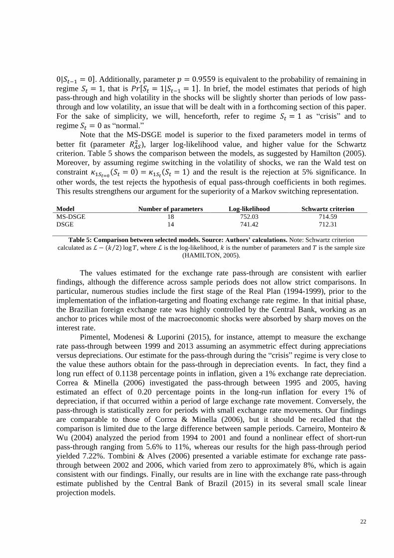
Note that the MS-DSGE model is superior to the fixed parameters model in terms of

better fit (parameter 𝑅𝐴𝑆2 ), larger log-likelihood value, and higher value for the Schwartz

criterion. Table 5 shows the comparison between the models, as suggested by Hamilton (2005).

Moreover, by assuming regime switching in the volatility of shocks, we ran the Wald test on

constraint 𝜅1𝑆𝑡=0(𝑆𝑡 = 0) = 𝜅1𝑆𝑡

(𝑆𝑡 = 1) and the result is the rejection at 5% significance. In

other words, the test rejects the hypothesis of equal pass-through coefficients in both regimes.

This results strengthens our argument for the superiority of a Markov switching representation.

Model Number of parameters Log-likelihood Schwartz criterion

MS-DSGE 18 752.03 714.59

DSGE 14 741.42 712.31

Table 5: Comparison between selected models. Source: Authors’ calculations. Note: Schwartz criterion

calculated as ℒ − (𝑘 2⁄ ) log 𝑇, where ℒ is the log-likelihood, 𝑘 is the number of parameters and 𝑇 is the sample size

(HAMILTON, 2005).

The values estimated for the exchange rate pass-through are consistent with earlier

findings, although the difference across sample periods does not allow strict comparisons. In

particular, numerous studies include the first stage of the Real Plan (1994-1999), prior to the

implementation of the inflation-targeting and floating exchange rate regime. In that initial phase,

the Brazilian foreign exchange rate was highly controlled by the Central Bank, working as an

anchor to prices while most of the macroeconomic shocks were absorbed by sharp moves on the

interest rate.

Pimentel, Modenesi & Luporini (2015), for instance, attempt to measure the exchange

rate pass-through between 1999 and 2013 assuming an asymmetric effect during appreciations

versus depreciations. Our estimate for the pass-through during the “crisis” regime is very close to

the value these authors obtain for the pass-through in depreciation events. In fact, they find a

long run effect of 0.1138 percentage points in inflation, given a 1% exchange rate depreciation.

Correa & Minella (2006) investigated the pass-through between 1995 and 2005, having

estimated an effect of 0.20 percentage points in the long-run inflation for every 1% of

depreciation, if that occurred within a period of large exchange rate movement. Conversely, the

pass-through is statistically zero for periods with small exchange rate movements. Our findings

are comparable to those of Correa & Minella (2006), but it should be recalled that the

comparison is limited due to the large difference between sample periods. Carneiro, Monteiro &

Wu (2004) analyzed the period from 1994 to 2001 and found a nonlinear effect of short-run

pass-through ranging from 5.6% to 11%, whereas our results for the high pass-through period

yielded 7.22%. Tombini & Alves (2006) presented a variable estimate for exchange rate pass-

through between 2002 and 2006, which varied from zero to approximately 8%, which is again

consistent with our findings. Finally, our results are in line with the exchange rate pass-through

estimate published by the Central Bank of Brazil (2015) in its several small scale linear

projection models.

23

Note that our long-run pass-through estimate (10.35%), even in a “crisis” period, is

considered relatively low by the criteria established by Goldfajn & Werlang (2000) and Belaisch

(2003), which implies that the economy has exhibited reasonable capacity to absorb exchange

rate shocks without direct pass-through to consumer inflation.

In order to analyze the results of the aggregate demand (IS) and the monetary policy

(MP) curves we should recall that our measure of the interest rate 𝑖𝑡 is calculated as the nominal

interest rate discounted for the long term real interest rate. In other words 𝑖𝑡 is the interest rate

“in excess” of the long term real rate. With that in mind, we find that the IS curve demonstrates

a strong response of output to the interest rate “in excess”, with parameter 𝜙 = 0.64740. In fact,

a relatively high value should be expected by theory. Our estimated parameter is much higher

than the calibration of Baele et al. (2015), of 𝜙 = 0.1, or the estimation of Gonçalves, Portugal

& Arágon (2016) who obtain 𝜙 = 0.4063, as both of these works use purely the nominal interest

rate as input to their models. Our findings indicate a strong reaction of aggregate demand to the

interest rate “in excess” of the long term real rate, which, in turn, shows an efficient channel for

monetary policy transmission in Brazil.

Regarding the monetary policy rule, we obtain an interest rate smoothing value of

𝜌𝑖 = 0.2515, which is relatively small in comparison to Bayesian estimations of DSGE models

such as Furlani, Portugal & Laurini (2010). Again, the difference in our interest rate input series

could explain a much slower smoothing coefficient. The Central Bank would be aiming to

smooth the nominal interest rate, which leads to a smaller smoothing of the interest rate that is

“in excess” of the long term real rate.

Parameter 𝛽, which stands for the response of the interest rate to inflation expectation,

was estimated at 0.7852 and indicates an activist response to inflation as it is significantly

different from zero.8 The interpretation that arises, in our case, is that the Central Bank would be

willing to raise the interest rate above the long term real rate for every positive shock in inflation

expectations. Anyway, our result is higher than the value estimated by Gonçalves, Portugal &

Arágon (2016), who used the nominal interest rate as input and obtained 𝛽 = 0.56 in their model

with fixed coefficient in the Taylor rule. These authors only manage to identify an activist

regime, with 𝛽 > 1 in their case, using a regime-switching model in the parameter 𝛽 itself.

The response of monetary policy to output is estimated at 𝛾 = 0.0117, and due to its high

standard deviation, it is not statistically different from zero. In any case, a positive value would

indicate that the Central Bank responds to output gap deviations, but that estimate should be

smaller than those of Palma & Portugal (2014) and Gonçalves, Portugal & Arágon (2016), for

example, again due to difference on the series for interest rates.

The exchange rate dynamics shows some positive autocorrelation in exchange rate

movements, with 𝜌𝑒 = 0.1488, but it is not significant. The volatility of shocks to the exchange

rate equation is by far the largest and the fit of the curve is almost irrelevant.

Parameter 𝛼 describes the law of motion of market expectations, and is very close to one,

implying that the model disregards market expectations assessed in the previous period.

According to Baele et al. (2015), this finding indicates that market expectations fully adjust to

rational expectations, and the slow dissemination of information does not appear to be important

in this process.

8 Note that, if we used the nominal interest rate as 𝑖𝑡 instead of the rate “in excess” of the long term real rate, the

activist regime would be characterized by 𝛽 > 1.

24

Table 6 shows the estimation results for the DSGE model without regime switching, for

the sake of comparison. The exchange rate pass-through coefficient, estimated in the AS curve,

is κ1 = 0.0419, which corresponds to a long-run effect of 0.0762 percentage points on inflation,

considering an exchange rate shock of 1%. Naturally, this value is within the interval between

the smallest and largest pass-through values estimated in the two-regime model. The other AS

curve parameters have similar values to those obtained for the MS-DSGE model. The relative

weight of endogenous persistence of inflation is a bit larger (𝛿 = 0.5497). In the meantime, the

output gap parameter has a heavier weight (𝜆 = 0.0887), but that is still nonsignificant. As

observed earlier, the Markov-switching model has larger log-likelihood value, larger value for

the Schwartz criterion, and better fit for the AS curve, indicating its superiority.

1. Parameters for the inflation curve

𝛿 𝜆 κ1

0.5497 0.0887 0.0419

0.1029 (0.000) 0.0776 (0.206) 0.0158 (0.014)

2. Parameters for the output gap curve

𝜇 𝜙

0.1231 0.6718

0.1015 (0.189) 0.3167 (0.044)

3. Monetary policy parameters

𝜌𝑖 𝛽 𝛾

0.2513 0.7857 0.0110

0.0711 (0.001) 0.1614 (0.000) 0.0541 (0.389)

4. Exchange rate dynamics parameters 5. Expectations formation

𝜌𝑒 𝛼

0.1488 1

0.1556 (0.250) 0.2819 (0.001)

6. Volatilities

𝜎𝐴𝑆 𝜎𝐼𝑆 𝜎𝑀𝑃 𝜎𝑒

0.0073 0.0108 0.0043 0.0950

0.0000 (0.000) 0.0000 (0.000) 0.0000 (0.003) 0.0017 (0.000)

7. Statistics

𝑅𝐴𝑆2 𝑅𝐼𝑆

2 𝑅𝑀𝑃2 𝑅𝑒

2 Log-likelihood

0.2688 0.5111 0.5383 0.0063 741.4227

Table 6: Parameters estimated for the structural model without regime switching. Source: Authors’

calculations. Note: the first row contains the parameter estimation and the second row contains the standard

deviation and p-values in brackets.

4.2 Specification and linearity tests

We ran the basic univariate specification tests on the standardized residuals of each

equation – serial autocorrelation, normality, and conditional variance – and linearity tests on the

MS-DSGE model. The results of the specification tests on standardized residuals are shown in

25

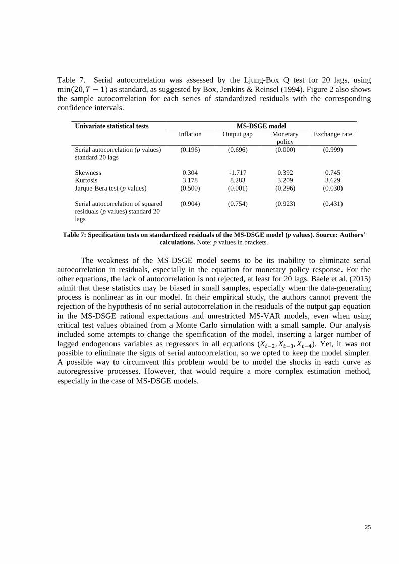
Table 7. Serial autocorrelation was assessed by the Ljung-Box Q test for 20 lags, using

min (20, 𝑇 − 1) as standard, as suggested by Box, Jenkins & Reinsel (1994). Figure 2 also shows

the sample autocorrelation for each series of standardized residuals with the corresponding

confidence intervals.

Univariate statistical tests MS-DSGE model

Inflation Output gap Monetary

policy

Exchange rate

Serial autocorrelation (p values)

standard 20 lags

(0.196) (0.696) (0.000) (0.999)

Skewness 0.304 -1.717 0.392 0.745

Kurtosis 3.178 8.283 3.209 3.629

Jarque-Bera test (p values) (0.500) (0.001) (0.296) (0.030)

Serial autocorrelation of squared

residuals (p values) standard 20

lags

(0.904) (0.754) (0.923) (0.431)

Table 7: Specification tests on standardized residuals of the MS-DSGE model (p values). Source: Authors’

calculations. Note: p values in brackets.

The weakness of the MS-DSGE model seems to be its inability to eliminate serial

autocorrelation in residuals, especially in the equation for monetary policy response. For the

other equations, the lack of autocorrelation is not rejected, at least for 20 lags. Baele et al. (2015)

admit that these statistics may be biased in small samples, especially when the data-generating

process is nonlinear as in our model. In their empirical study, the authors cannot prevent the

rejection of the hypothesis of no serial autocorrelation in the residuals of the output gap equation

in the MS-DSGE rational expectations and unrestricted MS-VAR models, even when using

critical test values obtained from a Monte Carlo simulation with a small sample. Our analysis

included some attempts to change the specification of the model, inserting a larger number of

lagged endogenous variables as regressors in all equations (𝑋𝑡−2, 𝑋𝑡−3, 𝑋𝑡−4). Yet, it was not

possible to eliminate the signs of serial autocorrelation, so we opted to keep the model simpler.

A possible way to circumvent this problem would be to model the shocks in each curve as

autoregressive processes. However, that would require a more complex estimation method,

especially in the case of MS-DSGE models.

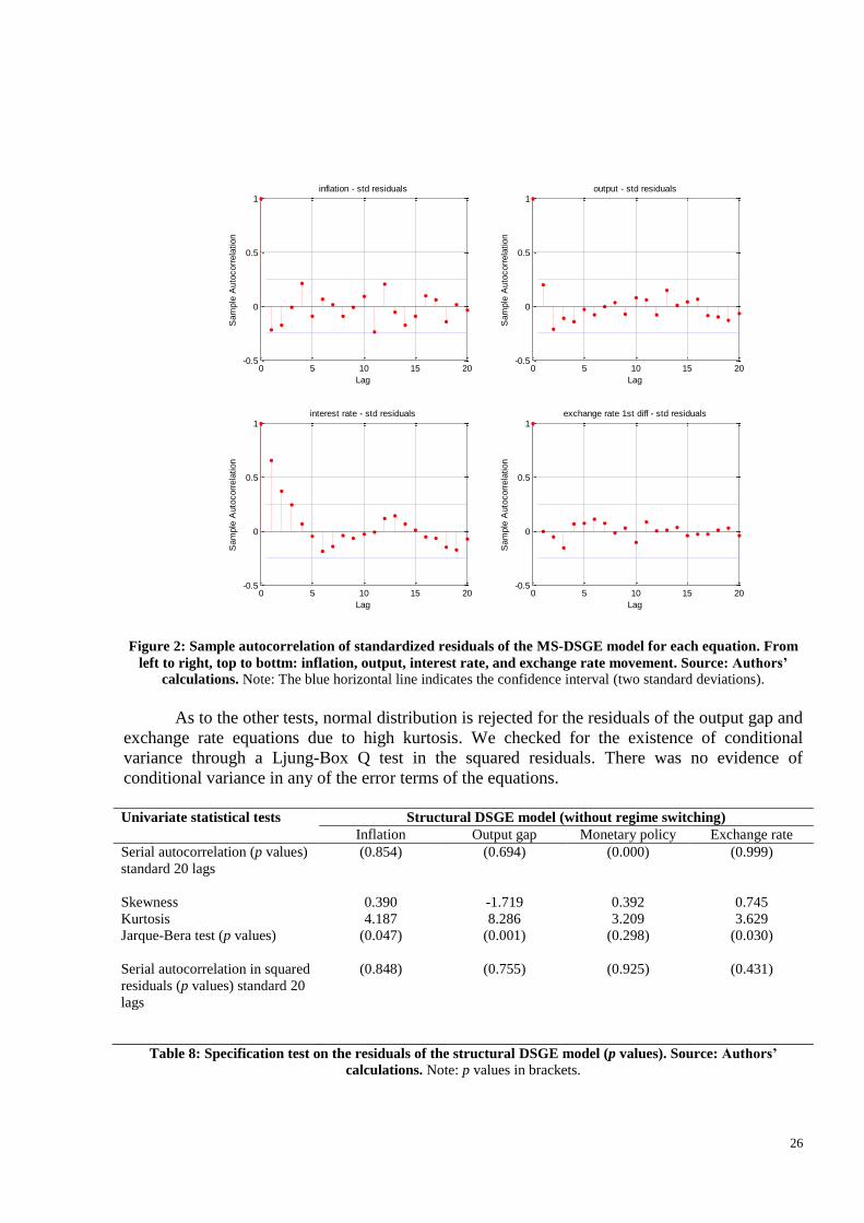
26

Figure 2: Sample autocorrelation of standardized residuals of the MS-DSGE model for each equation. From

left to right, top to bottm: inflation, output, interest rate, and exchange rate movement. Source: Authors’

calculations. Note: The blue horizontal line indicates the confidence interval (two standard deviations).

As to the other tests, normal distribution is rejected for the residuals of the output gap and

exchange rate equations due to high kurtosis. We checked for the existence of conditional

variance through a Ljung-Box Q test in the squared residuals. There was no evidence of

conditional variance in any of the error terms of the equations.

Univariate statistical tests Structural DSGE model (without regime switching)

Inflation Output gap Monetary policy Exchange rate

Serial autocorrelation (p values)

standard 20 lags

(0.854) (0.694) (0.000) (0.999)

Skewness 0.390 -1.719 0.392 0.745

Kurtosis 4.187 8.286 3.209 3.629

Jarque-Bera test (p values) (0.047) (0.001) (0.298) (0.030)

Serial autocorrelation in squared

residuals (p values) standard 20

lags

(0.848) (0.755) (0.925) (0.431)

Table 8: Specification test on the residuals of the structural DSGE model (p values). Source: Authors’

calculations. Note: p values in brackets.

0 5 10 15 20-0.5

0

0.5

1

Lag

Sam

ple

Auto

corr

ela

tion

inflation - std residuals

0 5 10 15 20-0.5

0

0.5

1

Lag

Sam

ple

Auto

corr

ela

tion

output - std residuals

0 5 10 15 20-0.5

0

0.5

1

Lag

Sam

ple

Auto

corr

ela

tion

interest rate - std residuals

0 5 10 15 20-0.5

0

0.5

1

Lag

Sam

ple

Auto

corr

ela

tion

exchange rate 1st diff - std residuals

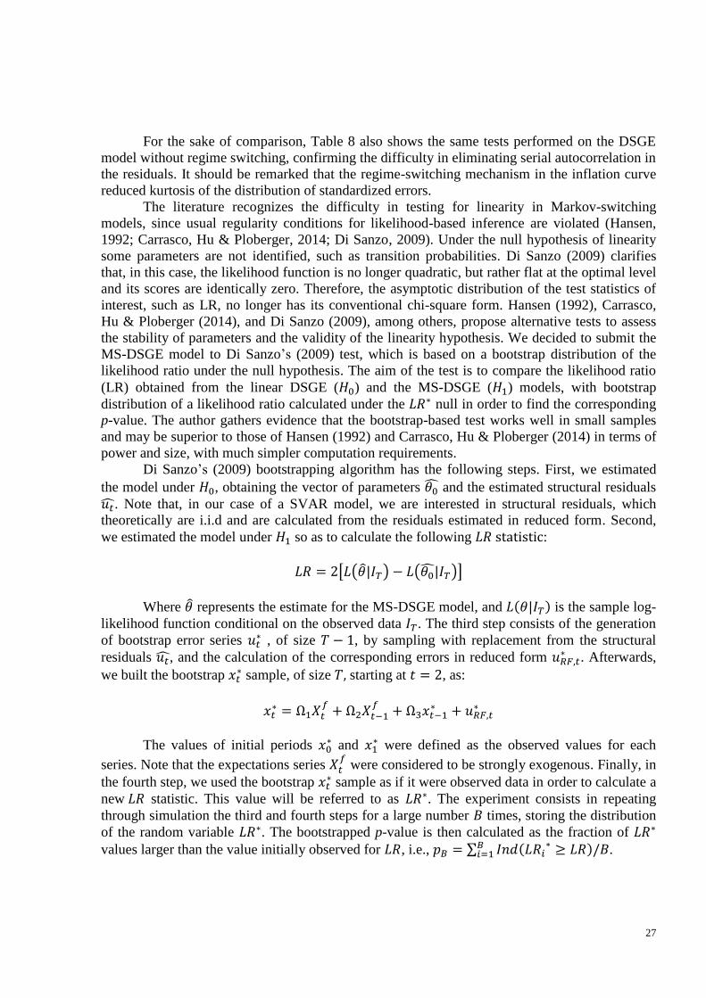
27

For the sake of comparison, Table 8 also shows the same tests performed on the DSGE

model without regime switching, confirming the difficulty in eliminating serial autocorrelation in

the residuals. It should be remarked that the regime-switching mechanism in the inflation curve

reduced kurtosis of the distribution of standardized errors.

The literature recognizes the difficulty in testing for linearity in Markov-switching

models, since usual regularity conditions for likelihood-based inference are violated (Hansen,

1992; Carrasco, Hu & Ploberger, 2014; Di Sanzo, 2009). Under the null hypothesis of linearity

some parameters are not identified, such as transition probabilities. Di Sanzo (2009) clarifies

that, in this case, the likelihood function is no longer quadratic, but rather flat at the optimal level

and its scores are identically zero. Therefore, the asymptotic distribution of the test statistics of

interest, such as LR, no longer has its conventional chi-square form. Hansen (1992), Carrasco,

Hu & Ploberger (2014), and Di Sanzo (2009), among others, propose alternative tests to assess

the stability of parameters and the validity of the linearity hypothesis. We decided to submit the

MS-DSGE model to Di Sanzo’s (2009) test, which is based on a bootstrap distribution of the

likelihood ratio under the null hypothesis. The aim of the test is to compare the likelihood ratio

(LR) obtained from the linear DSGE (𝐻0) and the MS-DSGE (𝐻1) models, with bootstrap

distribution of a likelihood ratio calculated under the 𝐿𝑅∗ null in order to find the corresponding

p-value. The author gathers evidence that the bootstrap-based test works well in small samples

and may be superior to those of Hansen (1992) and Carrasco, Hu & Ploberger (2014) in terms of

power and size, with much simpler computation requirements.

Di Sanzo’s (2009) bootstrapping algorithm has the following steps. First, we estimated

the model under 𝐻0, obtaining the vector of parameters 𝜃0̂ and the estimated structural residuals

𝑢�̂�. Note that, in our case of a SVAR model, we are interested in structural residuals, which

theoretically are i.i.d and are calculated from the residuals estimated in reduced form. Second,

we estimated the model under 𝐻1 so as to calculate the following 𝐿𝑅 statistic:

𝐿𝑅 = 2[𝐿(𝜃|𝐼𝑇) − 𝐿(𝜃0̂|𝐼𝑇)]

Where 𝜃 represents the estimate for the MS-DSGE model, and 𝐿(𝜃|𝐼𝑇) is the sample log-

likelihood function conditional on the observed data 𝐼𝑇. The third step consists of the generation

of bootstrap error series 𝑢𝑡∗ , of size 𝑇 − 1, by sampling with replacement from the structural

residuals 𝑢�̂�, and the calculation of the corresponding errors in reduced form 𝑢𝑅𝐹,𝑡∗ . Afterwards,

we built the bootstrap 𝑥𝑡∗ sample, of size 𝑇, starting at 𝑡 = 2, as:

𝑥𝑡∗ = Ω1𝑋𝑡

𝑓+ Ω2𝑋𝑡−1

𝑓+ Ω3𝑥𝑡−1

∗ + 𝑢𝑅𝐹,𝑡∗

The values of initial periods 𝑥0∗ and 𝑥1

∗ were defined as the observed values for each

series. Note that the expectations series 𝑋𝑡𝑓 were considered to be strongly exogenous. Finally, in

the fourth step, we used the bootstrap 𝑥𝑡∗ sample as if it were observed data in order to calculate a

new 𝐿𝑅 statistic. This value will be referred to as 𝐿𝑅∗. The experiment consists in repeating

through simulation the third and fourth steps for a large number 𝐵 times, storing the distribution

of the random variable 𝐿𝑅∗. The bootstrapped p-value is then calculated as the fraction of 𝐿𝑅∗

values larger than the value initially observed for 𝐿𝑅, i.e., 𝑝𝐵 = ∑ 𝐼𝑛𝑑(𝐿𝑅𝑖∗ ≥ 𝐿𝑅)/𝐵𝐵

𝑖=1 .

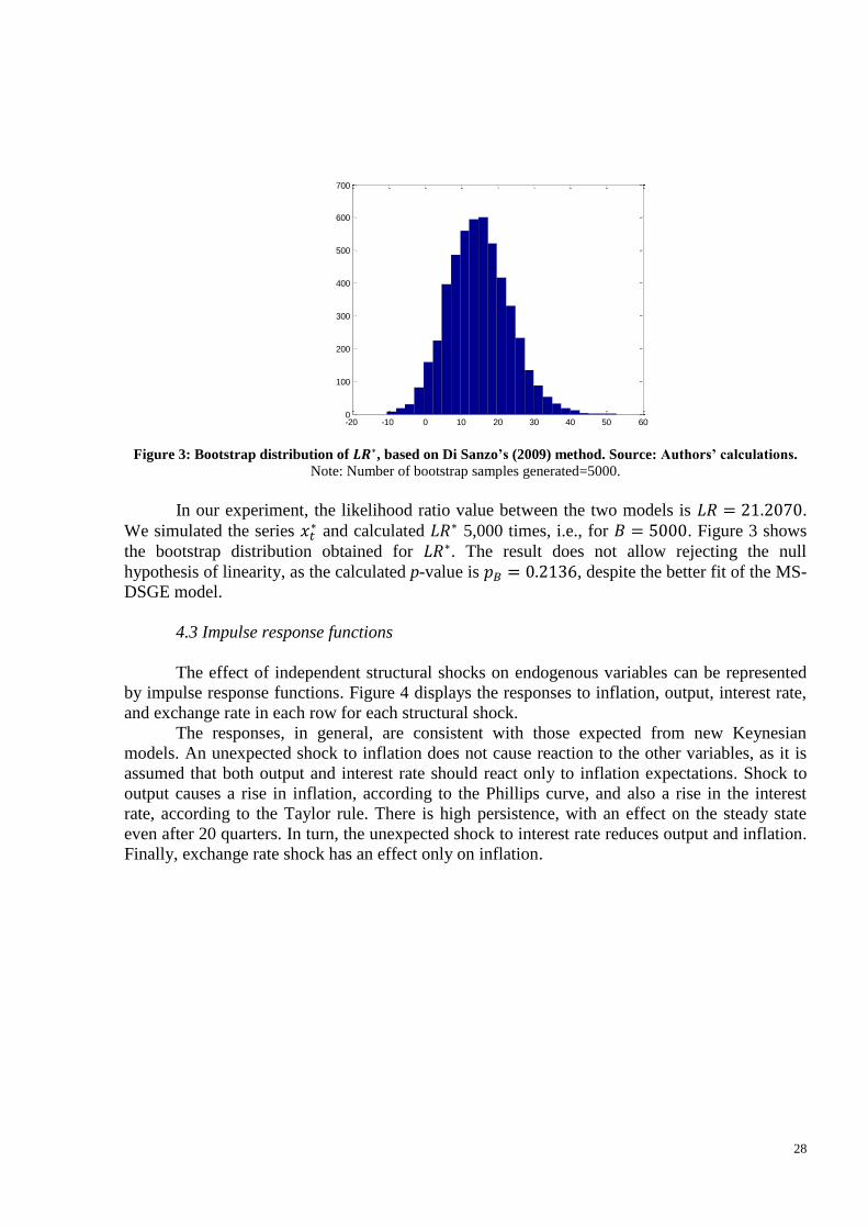
28

Figure 3: Bootstrap distribution of 𝑳𝑹∗, based on Di Sanzo’s (2009) method. Source: Authors’ calculations.

Note: Number of bootstrap samples generated=5000.

In our experiment, the likelihood ratio value between the two models is 𝐿𝑅 = 21.2070.

We simulated the series 𝑥𝑡∗ and calculated 𝐿𝑅∗ 5,000 times, i.e., for 𝐵 = 5000. Figure 3 shows

the bootstrap distribution obtained for 𝐿𝑅∗. The result does not allow rejecting the null

hypothesis of linearity, as the calculated p-value is 𝑝𝐵 = 0.2136, despite the better fit of the MS-

DSGE model.

4.3 Impulse response functions

The effect of independent structural shocks on endogenous variables can be represented

by impulse response functions. Figure 4 displays the responses to inflation, output, interest rate,

and exchange rate in each row for each structural shock.

The responses, in general, are consistent with those expected from new Keynesian

models. An unexpected shock to inflation does not cause reaction to the other variables, as it is

assumed that both output and interest rate should react only to inflation expectations. Shock to

output causes a rise in inflation, according to the Phillips curve, and also a rise in the interest

rate, according to the Taylor rule. There is high persistence, with an effect on the steady state

even after 20 quarters. In turn, the unexpected shock to interest rate reduces output and inflation.

Finally, exchange rate shock has an effect only on inflation.

-20 -10 0 10 20 30 40 50 600

100

200

300

400

500

600

700

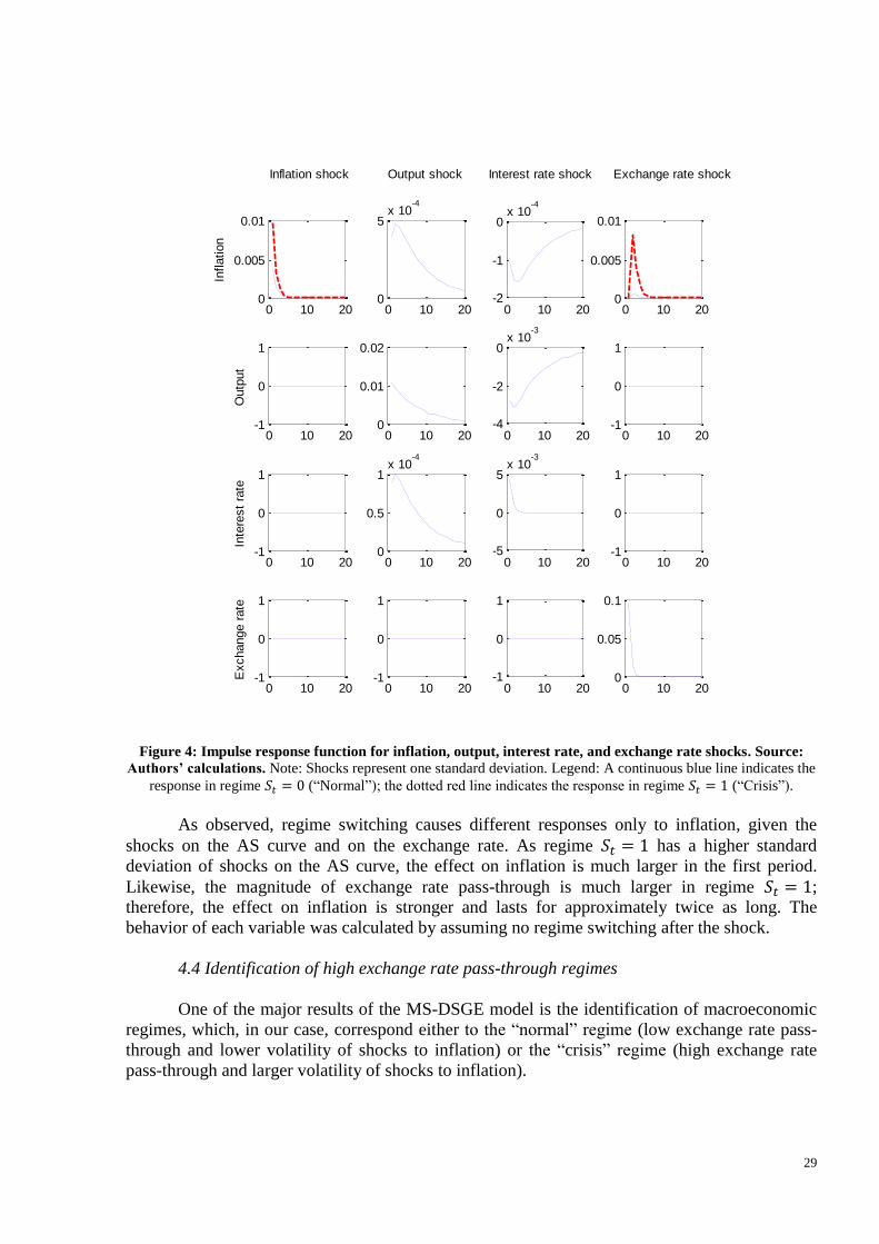
29

Figure 4: Impulse response function for inflation, output, interest rate, and exchange rate shocks. Source:

Authors’ calculations. Note: Shocks represent one standard deviation. Legend: A continuous blue line indicates the

response in regime 𝑆𝑡 = 0 (“Normal”); the dotted red line indicates the response in regime 𝑆𝑡 = 1 (“Crisis”).

As observed, regime switching causes different responses only to inflation, given the

shocks on the AS curve and on the exchange rate. As regime 𝑆𝑡 = 1 has a higher standard

deviation of shocks on the AS curve, the effect on inflation is much larger in the first period.

Likewise, the magnitude of exchange rate pass-through is much larger in regime 𝑆𝑡 = 1;

therefore, the effect on inflation is stronger and lasts for approximately twice as long. The

behavior of each variable was calculated by assuming no regime switching after the shock.

4.4 Identification of high exchange rate pass-through regimes

One of the major results of the MS-DSGE model is the identification of macroeconomic

regimes, which, in our case, correspond either to the “normal” regime (low exchange rate pass-

through and lower volatility of shocks to inflation) or the “crisis” regime (high exchange rate

pass-through and larger volatility of shocks to inflation).

0 10 200

0.005

0.01In

flation

0 10 20-1

0

1

Outp

ut

0 10 20-1

0

1

Inte

rest

rate

0 10 20-1

0

1

Exchange r

ate

0 10 200

5x 10

-4

0 10 200

0.01

0.02

0 10 200

0.5

1x 10

-4

0 10 20-1

0

1

0 10 20-2

-1

0x 10

-4

0 10 20-4

-2

0x 10

-3

0 10 20-5

0

5x 10

-3

0 10 20-1

0

1

0 10 200

0.005

0.01

0 10 20-1

0

1

0 10 20-1

0

1

0 10 200

0.05

0.1

Inflation shock Output shock Interest rate shock Exchange rate shock

30

As previously commented, both regimes demonstrate strong persistence, with a slightly

higher value attributed to the “normal” regime. In effect, the expected duration for the “normal”

cycle is 𝐸(𝐷|𝑆𝑡 = 0) = 24.0 quarters against 𝐸(𝐷|𝑆𝑡 = 1) = 22.7 quarters for the “crisis”

cycle.

The graphs in Figure 5 show filtered and smoothed probabilities for each regime

throughout the period. Note that the probabilities tend to concentrate around 1 or zero most of

the time, allowing for a plausible identification of regimes and confirming the usefulness of the

model. We are able to clearly identify two periods of high exchange rate pass-through and high

volatility of shocks to inflation, with duration between 6 and 14 quarters. Table 9 summarizes the

information on the beginning and end of each period, as well as on exchange rate movements

and accumulated inflation. The “crisis” regime totals 20 quarters, whereas the “normal” one

extends for 44 consecutive quarters.

Beginning End Duration

(quarters)

Identification Larger exchange rate

depreciation (in one

quarter)

Inflation

accumulated in

the period (IPCA)

2000/q1 2003/q2 14 Internet bubble (USA) and

domestic electoral crisis

31.4% 36.3%

2014/q3 2015/q4 6 Domestic political crisis 24.7% 12.9%

Table 9: Periods of high exchange rate pass-through and high volatility of shocks to inflation

identified by the MS-DSGE model. Source: Authors’ calculations.

During each cycle of the “crisis” regime, we find events of large exchange rate

depreciations, between 24.7% and 31.4%, in at least one of the quarters. Exchange rate shocks

above certain limits is one of the arguments presented by Correa & Minella (2006) for the

nonlinear behavior of the exchange rate pass-through, and this feature appears to be relevant

here. Note that mean exchange rate depreciation per quarter in “crisis” regimes reaches 5.22%

against a mean appreciation of 0.6% in “normal” regimes. Taken the whole sample, we observe a

mean depreciation of 1.2% per quarter. Notwithstanding, we identified some quarters in which

large exchange rate depreciations (above 10%) were not enough to characterize for a regime

switching in the pass-through. In other words, in a few cases, the economy appears to be able to

absorb the exchange rate shock without significant pass-through to inflation. For example, we

mention quarters 2011/q3 and 2012/q2, which had exchange rate depreciations of 17.2% and

10.3%, respectively.

As expected owing to the volatility of shocks on the AS curve, the mean inflation per

quarter during the “crisis” regime was 2.19%, a much higher value than the overall sample mean

of 1.60%, or the “normal” regime mean of 1.34%. Note that quarterly inflation exceeded 2% in

only one occasion (2004/q3) out of 44 in which the “normal” regime was active.

The first “crisis” cycle begins in 2000/q1 and lasts until mid-2003. The period is

characterized by several events that affected confidence in the Brazilian economy. First, the

transition to the floating exchange rate regime and the resulting sharp exchange rate depreciation

of 1999 launched a sudden increase in inflation for the following quarters. Second, the burst of

the US stock market bubble for high-tech companies in 2000 triggered considerable uncertainty

in international financial markets. Emerging market economies such as Brazil suffered capital

outflows, exchange rate depreciations and increased country risk premium. For instance, in the

third quarter of 2000, the Brazilian exchange rate depreciation amounted to 8.42%, with a peak

in inflation of 3.82%. In 2001/q3, we observe another strong exchange rate shock with further

31

increase in country risk premium9. Third, the Brazilian presidential elections of 2002 were

marked by a harsh confidence crisis. Markets were skeptical about the economic policy

intentions of the labour’s party presidential candidate, which was winning by far at the opinion

polls. The country risk premium increased considerably, reaching its peak in October 2002.10

The domestic currency experienced more than 50% depreciation in 2002 whereas yearly

inflation exceeded 12%. Indeed, inflation volatility only decreased at the end of 2003, as the new

government’s monetary and economic policies became consolidated as orthodox and adherent to

the principles of inflation-targeting.

0.0

0.2

0.4

0.6

0.8

1.0

2000 2001 2002 2003 2004 2005 2006 2007 2008 2009 2010 2011 2012 2013 2014 2015

Regime 0 - Filtered Prob.

Regime 0 - Smoothed Prob.

0.0

0.2

0.4

0.6

0.8

1.0

2000 2001 2002 2003 2004 2005 2006 2007 2008 2009 2010 2011 2012 2013 2014 2015

Regime 1 - Filtered Prob.

Regime 1 - Smoothed Prob.

Figure 5: Probabilities estimated for the MS-DSGE model for Regime 0 (at the top) and Regime 1 (at the

bottom). Source: Authors’ calculations. Note: Filtered probabilities in bars and smoothed probabilities in lines.

The following period, a long “normal” cycle, starts from mid-2003 and lasts until the end

of 2014, totaling 44 quarters in a row. Note that the exchange rate had quite a significant

appreciation from the beginning to the end of the period, 32% from 2003/q2 to 2014/q2,

although we observe a few quarters with depreciations higher than 10%.

The fact that the exchange rate pass-through was low in that period is consistent with the

assumption of Pimentel, Modenesi & Luporini (2015) about the asymmetric effect of exchange

rate movements. These authors found that appreciations tend to exhibit a much lower pass-

through level than depreciations of the same size. The total appreciation of 32% contributed to

keep inflation in low levels during this period. What is a striking fact is how come depreciations

9 The Embi+BR country risk premium index, measured by JP Morgan, had an average monthly value of 1,165 basis

points in October 2001. 10

The Embi+BR index had an average monthly value of 2,039 basis points in October 2002.

32

greater than 10% in some quarters did not triggered a higher level of pass-through? For example,

in the second and third quarters of 2008, during the onset of the international financial crisis, the

MS-DSGE model indicates an increase in the probability of a “crisis” cycle. The exchange rate

depreciation reaches 42% between 2008/q3 and q4, even though inflation is kept at relatively

low levels for both 2008 and the following year. As a result, the smoothed probabilities signal

that the economy appears to continue under a “normal” cycle. Thus, according to the model, the

sharp depreciation was not enough in order to substantially raise the level of pass-through. This

finding is in contrast with Correa & Minella (2006) who argue that exchange rate shocks above a

certain threshold would lead to a non-linear elevation on the level of pass-through. In our

opinion, there are two possible explanations for this phenomena. First, the sudden negative shock

in economic activity during 2008-2009 could be helping to alleviate inflation pressures, in line

with the Phillips curve assumptions. Second, there appears to be a role for confidence. The

“crisis” cycle is being signalled by the model during phases when the Brazilian economy appears

to be in distress, as it was the case from 2000-2003 and during the final cycle described below.

From the beginning of 2015, the MS-DSGE model began to clearly indicate a new

“crisis” cycle. We see a strong exchange rate depreciation (18.9%) in 2015/q1 and a constant rise

in inflation levels. The period is characterized by a deep downturn on economic activity in

Brazil, political crisis at the federal government level, and fiscal hardships. As a matter of fact,

the high persistence of inflation combined with an expansionary government budget, though

unsustainable, have hindered the actions of the monetary authority. Based on model findings,

one can expect that the 24.7% exchange rate shock of 2015/q3 will drag substantial effect on

inflation during the following quarters.

5. Conclusion

The present paper investigates the exchange rate pass-through in the Brazilian economy

during the floating exchange rate period using a Markov-switching DSGE (MS-DSGE) model.

Our basic hypothesis is of nonlinear behavior in the pass-through coefficient, combined with

regime switching in the volatility of shocks to the aggregate supply curve.

The estimated new Keynesian MS-DSGE model consists of four basic equations: the

aggregate supply (AS) curve or Phillips curve, the demand curve (IS), the reaction function of

the monetary authority, and one equation to describe the exchange rate dynamics. We propose to

model the exchange rate pass-through as a supply shock in the Phillips curve, following

Blanchard & Galí (2007). Our specification and estimation strategy was based on Baele et al.

(2015), although these authors analyse monetary policy regimes in the US in a closed economy

setting. Hence, the original model was extended to account for pass-through effects.

In particular, the estimation approach of Baele et al. (2015) uses survey market

expectations for inflation and output, in addition to observed macroeconomic series. The authors

argue that market agents have a rich information set, which may be useful in improving the

estimation. This reasoning is confirmed by Altug & Çakmakli (2016) who found a high

predictive power of survey-based expectations for inflation in Brazil. The method proposed by

Baele et al. (2015) allows us to transform the Markov-switching DSGE model in a structural

MS-VAR model, which can thus be estimated through conventional multivariate methods such

as Hamilton (1989, 1994) and Kim & Nelson (1999).

33

Our empirical results indicate that the exchange rate pass-through assumed two possible

states, or regimes, during the period. In the first regime, conveniently referred to as “normal”, the

pass-through is very low and statistically nonsignificant while, at the same time, the volatility of

shocks to inflation is also relatively low. On the other hand, in the second regime the pass-

through is relevant and significant, of about 10.3% in the long run, while the volatility of shocks

to inflation is also relatively higher. The high pass-through regime was named “crisis” as it

appears to occur in periods when the Brazilian economy was facing different types of distress, or

confidence crisis. The MS-DSGE model outperformed the linear specification by some usual

econometric criteria, such as the Schwartz criterion.

More specifically, the long-run effect estimated for the pass-through during “crisis”,

amounts to 0.1035 percentage points for consumer inflation, given a 1% exchange rate shock,

compared to 0.00057 percentage points in the “normal” regime. The standard deviation of the

shocks on the AS curve is estimated at 0.0096 for the “crisis” regime against 0.0043 in the

normal regime. The transition probabilities of the Markov chain indicate high persistence of both

regimes, with a slightly longer mean expected duration for “normal” cycles.

Our estimates for the nonlinear exchange rate pass-through in the Brazilian economy are

consistent with those obtained by Carneiro, Monteiro & Wu (2004), Correa & Minella (2006),

and Pimentel, Modenesi & Luporini (2015), taking into account the differences between the

periods of interest and the estimation method. It should be highlighted that the long-run pass-

through, of 10.3% even in the “crisis” regime, is relatively low according to the criteria set by

Goldfajn & Werlang (2000) and Belaisch (2003), which implies some reasonable capacity of the

economy to absorb exchange rate shocks without greater effect to consumer inflation.

The presence of regime switching in the volatility of shocks to inflation could be related

to the heteroskedasticity of inflation itself (Engle, 1982; Brunner & Hess, 1993) or to theoretical

arguments, such as Ball & Cecchetti’s (1990) and Owyang’s (2001). These authors point out that

higher inflation levels lead to higher volatility and greater uncertainty over future inflation

expectations. That is, unexpected inflation shocks increase uncertainty over future inflation and

causes larger volatility in inflation in the subsequent periods. The system would tend to remain

in a high volatility regime for some periods, which is well described in our findings.

The econometric specification tests indicate that the estimation method could not

eliminate serial autocorrelation of standardized residuals, especially from the interest rate curve.

We recognize that due to the simplicity of the method it cannot capture a possible autoregressive

structure of the shocks in each equation. Even Baele et al. (2015) faced this problem in their

empirical exercise. Moreover, the MS-DSGE model was submitted to Di Sanzo’s (2009)

bootstrapping linearity test, which could not reject the null hypothesis of linearity. In summary,

we should be cautious when interpreting the results.

Most of the remaining structural parameters of the MS-DSGE model yielded results in

line with theory. The AS curve parameters confirm the relevance of inflation expectations and

also indicate endogenous persistence. However, we cannot confirm a statistically significant

influence of output gap on inflation. The IS curve shows a smaller effect of output gap

expectations, and at the same time higher persistence of output. The response of output to the

real interest rate is remarkable, as expected, indicating an efficient monetary policy transmission

mechanism. The Taylor rule parameters reveal an active response of the interest rate to inflation

expectations. We note that our estimates differ from the usual literature as we use an interest rate

measure that is adjusted for the long term real interest rate.

34

The present study innovates in terms of methodology by using an MS-DSGE model for

the identification of nonlinearity of exchange rate pass-through in the Brazilian economy.

Previous studies usually sought to measure exchange rate pass-through directly in the Phillips

curve (Carneiro, Monteiro & Wu, 2004; Correa & Minella, 2006; Nogueira Jr, 2010; Pimentel,

Modenesi & Luporini, 2015) or in regressions specifically derived from microfoundations, such

as in Albuquerque & Portugal (2005). From an econometric perspective, the literature utilizes

nonlinear least squares (Carneiro, Monteiro & Wu, 2004), threshold models (Correa & Minella,

2006), smooth transition regression (Nogueira Jr, 2010), asymmetric SVAR models (Pimentel,

Modenesi & Luporini, 2015), or models with variable parameters (Albuquerque & Portugal,

2005). Our review of the extant literature did not find any publication that has used regime

switching models to assess exchange rate pass-through in the Brazilian economy, either for

modeling of the Phillips curve only or in broader models. On the other hand, our study differs

from that of Baele et al. (2015) as it assesses exchange rate pass-through instead of focusing on

the monetary policy rule. To achieve that end, we extended the original model by adding new

elements to the AS curve and a new equation to describe the exchange rate dynamics.

We make a novel contribution by identifying three phases, or cycles, for the pass-through

behaviour in the Brazilian economy during the inflation targeting period. Under our

interpretation, two “crisis” cycles, one at the beginning of the sample period (2000-2003) and the

other at the end (2015), are separated by a long “normal” cycle (2003-2014). The “crisis” cycles

appear to occur during periods where the Brazilian economy is under different types of stress. In

some cases, the economic strain was due to external factors, such as the emerging markets

confidence runs of 2000-2001. In other cases, political facts such as the crisis of 2002, triggered

by uncertainty during the presidential elections, or the political crisis of 2015, appear to be

related to exchange rate shocks complemented with a higher level of pass-through.

We conclude that the overall results of the MS-DSGE model are useful to the economic

analysis and interpretation of the exchange rate pass-through dynamics and its nonlinear effects

to a great extent. The model have shown to provide relevant information for inflation forecast,

especially during large exchange rate shocks, when there is more uncertainty about the effect of

the pass-through. For example, the econometrician forecasting inflation with a linear model

would assume a 7.6% level of pass-through in the long run. On the other hand, if the

econometrician is using a nonlinear model of our kind, there is room for a more subtle

interpretation. If the economy is under a “crisis” regime, the MS-DSGE model indicates that the

expected pass-through is substantially higher, of 10.35%. However, under a “normal” regime,

one could expect a long run pass-through roughtly null, of 0.57%. The difference between the

two model types carry obvious consequences for policy analysis and design.

Finally, our findings underscore the importance of assessing regime switching in certain

structural parameters of the Brazilian economy in new Keynesian models, corroborating, to some

extent, Gonçalves, Portugal & Arágon (2016). However, there exist some limitations concerning

the estimation method and the simple basic model used, with just four equations. The extension

to a more complete open economy model, such as proposed by Adolfson et al. (2007) or

Choudhri & Hakura (2015), and the application of more sophisticated econometric techniques

such as those of Foerster et al. (2014) would allow for more robust conclusions, and are thus

suggestions for future research.

35

References

ADOLFSON, M.; LASÉEN, S.; LINDÉ, J.; VILLANI, M. (2007) Bayesian estimation of an

open economy DSGE model with incomplete pass-through. Journal of International Economics,

v.72, p. 481-455, 2007.

ALBUQUERQUE, C. R.; PORTUGAL, M. S. (2005) Pass-through from exchange rate to prices

in Brazil: an analysis using time-varying parameters for the 1980-2002 period. Revista de

Economia, vol 12, n. 1, Banco Central del Uruguay, Mai. 2005.

ALTUG, S.; ÇAKMAKLI, C. (2016) Forecasting inflation using survey expectations and target

inflation: evidence for Brazil and Turkey. International Journal of Forecasting, v. 32, issue 1,

pp. 138-153, Jan.-Mar. 2016.

ALVES, S. A. L.; AREOSA, W. D. (2005) Targets and inflation dynamics. Banco Central do

Brasil Working Papers Series, n. 100, Oct. 2005.

AREOSA, W. D.; MEDEIROS, M. (2007). Inflation dynamics in Brazil: the case of a small open

economy. Brazilian Review of Econometrics, Vol. 27, n. 1, 2007, pp.131-166.

ARRUDA, E.; FERREIRA, R.; CASTELAR, I. (2008) Modelos lineares e não lineares da curva

de Phillips para previsão da taxa de inflação no Brasil. Anais do XXXVI Encontro Nacional de

Economia, Salvador, BA, Brasil. Dez. 2008.

BAELE, L.; BEKAERT, G.; CHO, S.; INGHELBRECHT, K.; MORENO, A. (2015)

Macroeconomic regimes. Journal of Monetary Economics, v. 70, Mar. 2015, pp. 51-71.

BALL, L.; CECCHETTI, S. (1990) Inflation and uncertainty at short and long horizons.

Brookings Papers on Economic Activity, v. 1, pp. 215-54, 1990.

BANCO CENTRAL DO BRASIL (2015). Relatório de Inflação. Brasilia: Banco Central do

Brasil, v. 17, n. 2, Jun. 2015.

BELAISCH, A. (2003) Exchange rate pass-through in Brazil. IMF Working Papers, WP/03/141,

Jul. 2003.

BELLONE, B. (2005) Classical estimation of multivariate Markov-switching models using

MSVARlib. EconWPA, Econometrics 0508017, 2005.

BIANCHI, F. (2013). Regime switches, agents’ beliefs, and post-World War II U.S.

macroeconomic dynamics. Review of Economic Studies, 80 (2), pp. 463-490.

BLANCHARD, O.; GALÍ, J. (2007) Real wage rigidities and the New Keynesian model.

Journal of Money, Credit and Banking, v. 39, pp. 35-65, 2007.

BOX, G. E. P.; JENKINS, G. M. ; REINSEL, G. C. (1994) Time Series Analysis: forecasting

and control. 3rd ed. Englewood Cliffs, NJ: Prentice Hall, 1994.

36

BRUNNER, A. D.; HESS, G. D. (1993) Are Higher Levels of Inflation Less Predictable? A

State-Dependent Conditional Heteroscedasticity Approach. Journal of Business & Economic

Statistics, vol. 11, Issue. 2, 1993.

CALVO, G. A. (1983) Staggered Prices in a Utility-Maximizing Framework. Journal of

Monetary Economics, v. 12 (3), pp. 383-398, 1983.

CARNEIRO, D. D.; MONTEIRO, A. M. D.; WU, T. Y. H. (2004) Mecanismos não-lineares de

repasse cambial para o IPCA. Revista de Economia e Administração, v.3, n.1, pp.01-14, Jan-Mar

2004.

CARRASCO, M.; HU, L.; PLOBERGER, W. (2014) Optimal test for Markov switching

parameters. Econometrica, v. 82, n. 2, Mar. 2014, pp. 765-784.

CHO, S. (2014) Characterizing Markov-switching rational expectation models. University of

Indiana Economics Department Spring Working Papers. Available at: http:

//www.indiana.edu/~econdept/workshops/Spring_2013_Papers/SEONGHOON%20CHO.pdf.

CHO, S.; MORENO, A. (2011) The forward method as a solution refinement in rational

expectations models. Journal of Economic Dynamics and Control, v. 25 (3), pp. 257-327.

CHOI, J.; HUR, J. (2015) An examination of macroeconomic fluctuations in Korea exploiting a

Markov-switching DSGE approach. Economic Modelling, v. 51, Dec. 2015, pp. 183-199.

CHOUDHRI, E. U.; HAKURA, D. S. (2015) The exchange rate pass-through to import and

export prices: the role of nominal rigidities and currency choice. Journal of International Money

and Finance, v. 51, Mar. 2015, pp. 1-25.

CORREA, A. S.; MINELLA, A. (2006) Nonlinear mechanisms of the exchange rate pass-

through: a Phillips Curve model with threshold for Brazil. Banco Central do Brasil Working

Papers Series, n. 122, Nov. 2006.

DE CASTRO, M.; GOUVEA, S.; MINELLA, A.; SANTOS, R.; SOBRINHO, N. (2011)

SAMBA: Stochastic analytical model with a Bayesian approach. Banco Central do Brasil

Working Papers Series, n. 239.

DI SANZO, S. (2009) Testing for linearity in Markov switching models: a bootstrap approach.

Statistical Methods and Applications, v. 18, issue 2, Jul. 2009, pp. 153-168.

DIXIT, A. (1989) Hysteresis, import penetration, and exchange rate pass-through. The Quarterly

Journal of Economics, v. 104, n. 2, pp. 205-228, May 1989.

DONAYRE, L.; PANOVSKA, I. (2016) State-dependent exchange rate pass-through behavior.

Journal of International Money and Finance, v. 64, Jun. 2016, pp. 170-195.

ENGLE, R. F. (1982) Autoregressive conditional heteroscedasticity with estimates of the

variance of United Kingdom inflation. Econometrica, vol. 50, no. 4, July, 1982, pp.987-1007.

FARMER, R. E. A.; WAGGONER, D. F.; ZHA, T. (2009) Understanding Markov-switching

rational expectations models. Journal of Economic Theory, v. 144, pp. 1849-1867, 2009.

FARMER, R. E. A.; WAGGONER, D. F.; ZHA, T. (2010) Generalizing the Taylor principle: a

comment. American Economic Review, 100 (1), pp. 608-617, 2010.

37

FARMER, R. E. A.; WAGGONER, D. F.; ZHA, T. (2011) Minimal state variable solutions to

Markov-switching rational expectations models. Journal of Economic Dynamics & Control, v.

35, pp. 2150-2166, 2011.

FASOLO, A. M.; PORTUGAL, M. S. (2004) Imperfect rationality and inflationary inertia: a

new estimation of the Phillips curve for Brazsil. Estudos Econômicos, v. 34, n. 4, pp. 725-779,

Out-Dez, 2004.

FERNÁNDEZ-VILLAVERDE, J. (2009) The econometrics of DSGE models. NBER Working

Paper, No. 14677, Jan. 2009.

FERNÁNDEZ-VILLAVERDE, J.; GUERRÓN-QUINTANA, P.; RUBIO-RAMÍREZ, J. F.

(2010) Fortune or virtue: time-variant volatilities versus parameter drifting in U.S. data. NBER

Working Paper, No. 15928, Apr. 2010.

FIGUEIREDO, F. M. R.; GOUVEA, S. (2011) Repasse Cambial para a Inflação: o papel da

rigidez de preços. In: BANCO CENTRAL DO BRASIL (2011). Dez Anos de Metas para

Inflação 1999-2009. Brasília: Banco Central do Brasil, 2011.

FOERSTER, A.; RUBIO-RAMÍREZ, J. F.; WAGGONER, D.; ZHA, T. (2014) Perturbation

methods for Markov-switching models. NBER Working Paper, No. 20390, Aug. 2014.

FURLANI, L. G. C.; PORTUGAL, M. S.; LAURINI, M. P. (2010) Exchange rate movements

and monetary policy in Brazil: econometric and simulation evidence. Economic Modelling, v. 7,

issue 1, PP. 284-295, Jan. 2010.

GALÍ, J. (2008) Monetary Policy, Inflation, and the Business Cycle: an introduction to the New

Keynesian framework. Princeton University Press: Princeton, NJ, 2008.

GOLDFAJN, I.; WERLANG, S. R. C. (2000) The pass-through from depreciation to inflation: a

panel study. Banco Central do Brasil Working Papers Series, n. 5, Set. 2000.

GONÇALVES, C. C. S.; PORTUGAL, M. S.; ARÁGON, E. K. S. B. (2016) Assessing Brazilian

macroeconomic dynamics using a Markov-switching DSGE model. EconomiA, Mar. 2016.

HAMILTON, J. D. (1989) A new approach to the economic analysis of nonstationary time series

and the business cycle. Econometrica, v. 57, n. 2, pp 357-384, Mar. 1989.

HAMILTON, J. D. (1994) Time Series Analysis. Princeton University Press, 1994.

HAMILTON, J. D. (2005) What’s real about the Business Cycle? Federal Reserve Bank of St.

Louis Review, 87 (4), pp. 435-452, Jul-Aug 2005.

HAMILTON, J. D. (2014) Macroeconomic regimes and regime shifts, in Taylor, J. B. & Uhlig,

H. (Eds.) Handbook of Macroeconomics, Vol. 2.

HANSEN, B. E. (1992) The likelihood ratio test under nonstandard conditions: testing the

Markov switching model of GNP. Journal of Applied Econometrics, v. 7, Dec. 1992, pp. S61-

S82.

HOLMES, M. J. (2009) The response of exchange rate pass-through to the macroeconomic

environment. The Open Business Journal, v. 2, pp. 1-6, 2009.

38

IBOSHI, H. (2016) Monetary policy regime shifts under the zero lower bound: an application of

a stochastic rational expectations equilibrium to a Markov switching DSGE model. Economic

Modelling, v. 52, part A, Jan. 2016, pp. 186-205.

KHEMIRI, R.; ALI, M. S. B. (2012) Exchange rate pass-through and inflation dynamics in

Tunisia: a Markov-switching approach. Economics E-journal Discussion Paper, n. 2012-39,

Aug., 2012.

KOHLSCHEEN, E. (2010) Emerging Floaters: pass-throughs and (some) new commodity

currencies. Banco Central do Brasil Working Papers Series, n. 224, Nov. 2010.

KROLZIG, H.M. (1997) Markov-Switching Vector Autoregressions: modelling, statistical

inference and application to business cycle analysis. Springer-Verlag: Berlin, 1997.

LARUE, B.; GERVAIS, J.; RANCOURT, Y. (2010) Exchange rate pass-through, menu costs

and threshold cointegration. Empirical Economics, v. 38, issue 1, Feb. 2010, pp. 171-192.

LIU, P.; MUMTAZ, H. (2010) Evolving macroeconomic dynamics in a small open economy: an

estimated Markov-switching DSGE model for the United Kingdom. Bank of England Working

Paper No. 397.

MAIH, J. (2015) Efficient perturbation methods for solving regime-switching DSGE models.

Norges Bank Working Paper, Jan. 2015.

MANKIW, N. G.; REIS, R. (2002) Sticky information versus sticky prices: a proposal to replace

the new Keynesian Phillips curve. Quarterly Journal of Economics, 117 (4), pp. 251-301.

MAZALI, A. A.; DIVINO, J. A. (2010) Real wage rigidity and the new Phillips curve: the

Brazilian case. Revista Brasileira de Economia, v.64, n.3, pp. 291-306, Jul-Sep 2010.

MINELLA, A.; DE FREITAS, P. S.; GOLDFAJN, I.; MUINHOS, M. K. (2003) Inflation

Targeting in Brazil: Constructing Credibility under Exchange Rate Volatility. Banco Central do

Brasil Working Papers Series, n. 77, Jul. 2003.

NOGUEIRA JR, R. P. (2010) Inflation environment and lower exchange rate pass-through in

Brazil: is there a relationship? Revista Brasileira de Economia, v. 64, n. 1, pp. 49-56, Jan.-Mar.

2010.

OLIVEIRA, L.; FEIJÓ, F. T. (2015) Curva de Phillips com mudança de regime markoviano:

uma análise da economia brasileira para o período 1995-2014. Anais do XLIII Encontro

Nacional de Economia da ANPEC. Florianópolis, SC, Brasil. Dez., 2015.

OWYANG, M. T. (2001) Persistence, excess volatility, and volatility clusters in inflation.

Federal Reserve Bank of St. Louis Review, v. 83, n. 6, pp. 41-52, Nov-Dec 2001.

PALMA, A. A.; PORTUGAL, M. S. (2014) Preferences of the Central Bank of Brazil under the

inflation targeting regime: estimation using a DSGE model for a small open economy. Journal of

Policy Modeling, v. 36, issue 5, pp. 824-839, Sep-Oct 2014.

PIMENTEL, D. M.; MODENESI, A. M.; LUPORINI, V. (2015) Assimetrias no repasse cambial

para a inflação: uma análise empírica para o Brasil (1999 a 2013). Anais do XVIII Encontro de

Economia da Região Sul ANPEC Sul. Porto Alegre, RS, Brasil. Jun., 2015.

39

RAZAFINDRABE, T. M. (2016) A multi-country DSGE model with incomplete exchange rate

pass-through: an application for the Euro-area. Economic Modelling, v. 52, part A, Jan. 2016, pp.

78-100.

RODRIGUES, W. G.; MORI, R. (2015) Mudanças de regimes na função de reação do Banco

Central do Brasil: uma abordagem utilizando Markov regime switching. Anais do XLIII

Encontro Nacional de Economia da ANPEC. Florianópolis, SC, Brasil. Dez., 2015.

ROMER, D. (2011) Advanced Macroeconomics, 4th Edition. McGraw-Hill: New York, 2011.

SACHSIDA, A. (2013) Inflação, desemprego e choques cambiais: uma revisão da literatura

sobre a Curva de Phillips no Brasil. Revista Brasileira de Economia, v. 67, n.4, pp. 521-531,

Out.-Dez. 2013.

SILVEIRA, M. A. C. (2008) Using a Bayesian approach to estimate and compare New

Keynesian DSGE models for the Brazilian economy: the role for endogenous persistence.

Revista Brasileira de Economia, v. 62, n. 3, pp. 333-357, Jul-Sep 2008.

SIMS, C. (2002) Solving linear rational expectations models. Computational Economics, v. 20

(1-2), pp. 1-20.

SIMS, C.; ZHA, T. (2006) Were there regime switches in U.S. monetary policy? American

Economic Review, 91(1), pp.54-81.

TAYLOR, J. (2000) Low inflation, pass-through and the pricing power of firms. European

Economic Review, 44, pp. 1389-1408, 2000.

TOMBINI, A. A.; ALVES, S. A. L. (2006) The recent Brazilian disinflation process and costs.

Banco Central do Brasil Working Papers Series, n. 109, Jun. 2006.

TRISTÃO, T. S.; TORRENT, H. S. (2015) Relações não lineares na curva de Phillips: uma

abordagem semi-paramétrica. Economia Aplicada, v. 19, n. 4, 2015, pp. 679-703.

VIEIRA, H. P.; PEREIRA, P. V. (2013) A study of the Brazilian business cycles (1900-2012).

Brazilian Review of Econometrics, v. 33, no 2, pp. 123-143, Nov. 2013.

WINKELRIED, D. (2014) Exchange rate pass-through and inflation targeting in Peru. Empirical

Economics, v. 46, issue 4, Jun. 2014, pp. 1181-1196.

Exchange Rate Pass-Through in Brazil: a Markov Switching ... de Economa/PORTUGAL... · example,...

Documents

Transcript of Exchange Rate Pass-Through in Brazil: a Markov Switching ... de Economa/PORTUGAL... · example,...