Excel Windows & MacÞItZ Excel 50 Excel Windows & MacÞItZ ...
Upload
pauline-bogador-mayordomoCategory
view
4download
0description
ICT Skills Enhancement Training for Brgy. Officials of Municipality of Badiangan July 5, 12, 19, 26,
August 2 & 9 2013
Lesson 1: Entering Text and NumbersThe Microsoft Excel WindowMicrosoft Excel is an electronic spreadsheet. You can use it to organize your data into rows and columns. You can also use it to perform mathematical calculations quickly. This tutorial teaches Microsoft Excel basics. Although knowledge of how to navigate in a Windows environment is helpful, this tutorial was created for the computer novice.This lesson will introduce you to the Excel window. You use the window to interact with Excel. To begin this lesson, start Microsoft Excel 2007. The Microsoft Excel window appears and your screen looks similar to the one shown here.
The Microsoft Office ButtonIn the upper-left corner of the Excel 2007 window is the Microsoft Office button. When you click the button, a menu appears. You can use the menu to create a new file, open an existing file, save a file, and perform many other tasks.
The Quick Access ToolbarNext to the Microsoft Office button is the Quick Access toolbar. The Quick Access toolbar gives you with access to commands you frequently use. By default, Save, Undo, and Redo appear on the Quick Access toolbar. You can use Save to save your file, Undo to roll back an action you have taken, and Redo to reapply an action you have rolled back.
The Title Bar
Basic Computer Operation Skills Training (BCOST)
ICT Skills Enhancement Training for Brgy. Officials of Municipality of Badiangan July 5, 12, 19, 26,
August 2 & 9 2013
Next to the Quick Access toolbar is the Title bar. On the Title bar, Microsoft Excel displays the name of the workbook you are currently using. At the top of the Excel window, you should see "Microsoft Excel - Book1" or a similar name.
The RibbonYou use commands to tell Microsoft Excel what to do. In Microsoft Excel 2007, you use the Ribbon to issue commands. The Ribbon is located near the top of the Excel window, below the Quick Access toolbar. At the top of the Ribbon are several tabs; clicking a tab displays several related command groups. Within each group are related command buttons. You click buttons to issue commands or to access menus and dialog boxes. You may also find a dialog box launcher in the bottom-right corner of a group. When you click the dialog box launcher, a dialog box makes additional commands available.
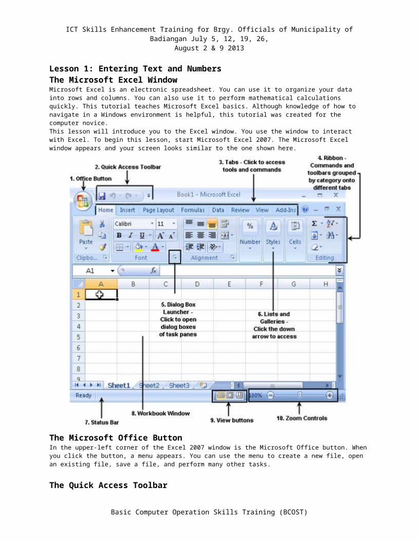
Worksheets
Microsoft Excel consists of worksheets. Each worksheet contains columns and rows. The columns are lettered A to Z and then continuing with AA, AB, AC and so on; the rows are numbered 1 to 1,048,576. The number of columns and rows you can have in a worksheet is limited by your computer memory and your system resources.The combination of a column coordinate and a row coordinate make up a cell address. For example, the cell located in the upper-left corner of the worksheet is cell A1, meaning column A, row 1. Cell E10 is located under column E on row 10. You enter your data into the cells on the worksheet.
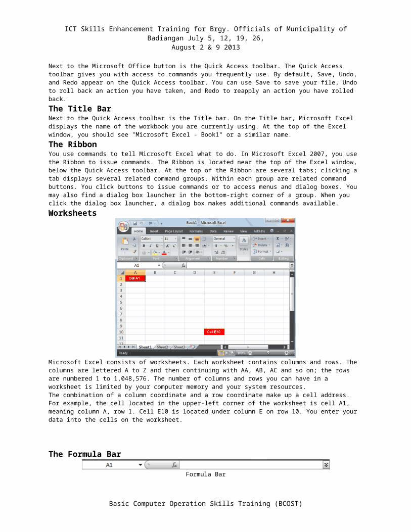
The Formula Bar
Formula BarIf the Formula bar is turned on, the cell address of the cell you are in displays in the Name box which is located on the left side of the Formula bar. Cell entries display on the right side of the Formula bar. If you do not see the Formula bar in your window, perform the following steps:
1. Choose the View tab.2. Click Formula Bar in the Show/Hide group. The Formula bar appears.
Note: The current cell address displays on the left side of the Formula bar.
The Status Bar
The Status bar appears at the very bottom of the Excel window and provides such information as the sum, average, minimum, and maximum value of selected numbers. You can change what displays on the Status bar by right-clicking on the Status bar and selecting the options you want from the Customize Status Bar menu. You click a menu item to select it. You click it again to deselect it. A check mark next to an item means the item is selected.
Basic Computer Operation Skills Training (BCOST)

ICT Skills Enhancement Training for Brgy. Officials of Municipality of Badiangan July 5, 12, 19, 26,
August 2 & 9 2013
Move Around a WorksheetBy using the arrow keys, you can move around your worksheet. You can use the down arrow key to move downward one cell at a time. You can use the up arrow key to move upward one cell at a time. You can use the Tab key to move across the page to the right, one cell at a time. You can hold down the Shift key and then press the Tab key to move to the left, one cell at a time. You can use the right and left arrow keys to move right or left one cell at a time. The Page Up and Page Down keys move up and down one page at a time. If you hold down the Ctrl key and then press the Home key, you move to the beginning of the worksheet.
Go To Cells QuicklyThe following are shortcuts for moving quickly from one cell in a worksheet to a cell in a different part of the worksheet.EXERCISE 1Go to -- F5The F5 function key is the "Go To" key. If you press the F5 key, you are prompted for the cell to which you wish to go. Enter the cell address, and the cursor jumps to that cell.
1. Press F5. The Go To dialog box opens.2. Type J3 in the Reference field.3. Press Enter. Excel moves to cell J3.
Go to -- Ctrl+GYou can also use Ctrl+G to go to a specific cell.
1. Hold down the Ctrl key while you press "g" (Ctrl+g). The Go To dialog box opens.2. Type C4 in the Reference field.3. Press Enter. Excel moves to cell C4.
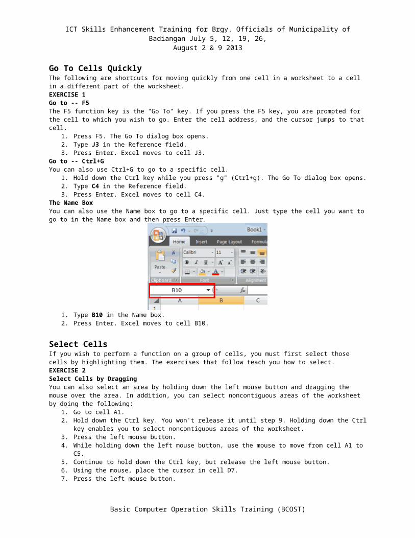
The Name BoxYou can also use the Name box to go to a specific cell. Just type the cell you want to go to in the Name box and then press Enter.
Basic Computer Operation Skills Training (BCOST)
ICT Skills Enhancement Training for Brgy. Officials of Municipality of Badiangan July 5, 12, 19, 26,
August 2 & 9 2013
1. Type B10 in the Name box.2. Press Enter. Excel moves to cell B10.
Select CellsIf you wish to perform a function on a group of cells, you must first select those cells by highlighting them. The exercises that follow teach you how to select.EXERCISE 2Select Cells by DraggingYou can also select an area by holding down the left mouse button and dragging the mouse over the area. In addition, you can select noncontiguous areas of the worksheet by doing the following:
1. Go to cell A1.2. Hold down the Ctrl key. You won't release it until step 9. Holding down the Ctrl key enables you to select
noncontiguous areas of the worksheet.3. Press the left mouse button.4. While holding down the left mouse button, use the mouse to move from cell A1 to C5.5. Continue to hold down the Ctrl key, but release the left mouse button.6. Using the mouse, place the cursor in cell D7.7. Press the left mouse button.8. While holding down the left mouse button, move to cell F10. Release the left mouse button.9. Release the Ctrl key. Cells A1 to C5 and cells D7 to F10 are selected.10. Press Esc and click anywhere on the worksheet to remove the highlighting.
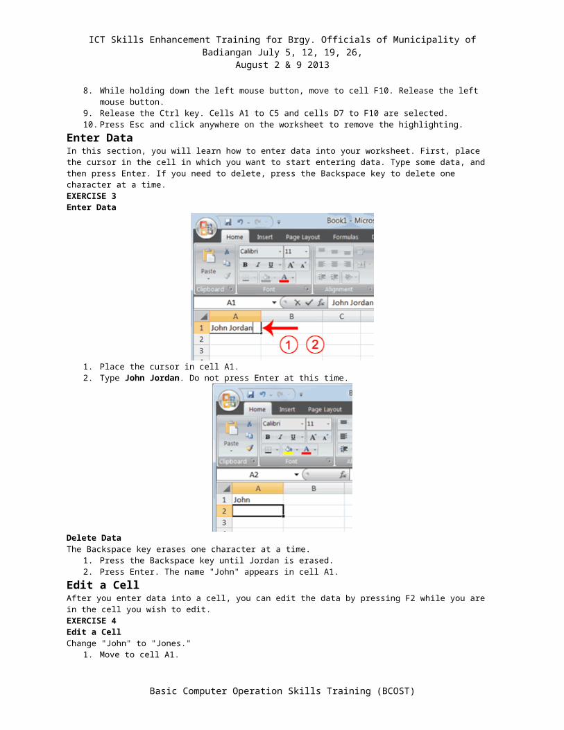
Enter DataIn this section, you will learn how to enter data into your worksheet. First, place the cursor in the cell in which you want to start entering data. Type some data, and then press Enter. If you need to delete, press the Backspace key to delete one character at a time.EXERCISE 3Enter Data
1. Place the cursor in cell A1.2. Type John Jordan. Do not press Enter at this time.
Basic Computer Operation Skills Training (BCOST)
ICT Skills Enhancement Training for Brgy. Officials of Municipality of Badiangan July 5, 12, 19, 26,
August 2 & 9 2013
Delete DataThe Backspace key erases one character at a time.
1. Press the Backspace key until Jordan is erased.2. Press Enter. The name "John" appears in cell A1.
Edit a CellAfter you enter data into a cell, you can edit the data by pressing F2 while you are in the cell you wish to edit.EXERCISE 4Edit a CellChange "John" to "Jones."
1. Move to cell A1.2. Press F2.3. Use the Backspace key to delete the "n" and the "h."4. Type nes.5. Press Enter.
Alternate Method: Editing a Cell by Using the Formula BarYou can also edit the cell by using the Formula bar. You change "Jones" to "Joker" in the following exercise.
1. Move the cursor to cell A1.2. Click in the formula area of the Formula bar.3. Use the backspace key to erase the "s," "e," and "n."4. Type ker.5. Press Enter.
Alternate Method: Edit a Cell by Double-Clicking in the CellYou can change "Joker" to "Johnson" as follows:
1. Move to cell A1.2. Double-click in cell A1.3. Press the End key. Your cursor is now at the end of your text.4. Use the Backspace key to erase "r," "e," and "k."5. Type hnson.6. Press Enter.
Change a Cell EntryTyping in a cell replaces the old cell entry with the new information you type.
1. Move the cursor to cell A1.2. Type Cathy.3. Press Enter. The name "Cathy" replaces "Johnson."
Wrap TextWhen you type text that is too long to fit in the cell, the text overlaps the next cell. If you do not want it to overlap the next cell, you can wrap the text.EXERCISE 5Wrap Text
1. Move to cell A2.2. Type Text too long to fit.
Basic Computer Operation Skills Training (BCOST)

ICT Skills Enhancement Training for Brgy. Officials of Municipality of Badiangan July 5, 12, 19, 26,
August 2 & 9 2013
3. Press Enter.
4. Return to cell A2.5. Choose the Home tab.
6. Click the Wrap Text button . Excel wraps the text in the cell.
Delete a Cell EntryTo delete an entry in a cell or a group of cells, you place the cursor in the cell or select the group of cells and press Delete.EXERCISE 6Delete a Cell Entry
1. Select cells A1 to A2.2. Press the Delete key.
Save a FileThis is the end of Lesson1. To save your file:
1. Click the Office button. A menu appears.2. Click Save. The Save As dialog box appears.3. Go to the directory in which you want to save your file.4. Type Lesson1 in the File Name field.5. Click Save. Excel saves your file.
Close ExcelClose Microsoft Excel.
1. Click the Office button. A menu appears.2. Click Close. Excel closes.
Lesson 2: Entering Excel Formulas and Formatting Data
Lesson 1 familiarized you with the Excel 2007 window, taught you how to move around the window, and how to enter data. A major strength of Excel is that you can perform mathematical calculations and format your data. In this lesson, you learn how to perform basic mathematical calculations and how to format text and numerical data. To start this lesson, open Excel.
Perform Mathematical CalculationsIn Microsoft Excel, you can enter numbers and mathematical formulas into cells. Whether you enter a number or a formula, you can reference the cell when you perform mathematical calculations such as addition, subtraction, multiplication, or division. When entering a mathematical formula, precede the formula with an equal sign. Use the following to indicate the type of calculation you wish to perform:+ Addition- Subtraction* Multiplication/ Division^ ExponentialIn the following exercises, you practice some of the methods you can use to move around a worksheet and you learn how to perform mathematical calculations. Refer to Lesson 1 to learn more about moving around a worksheet.EXERCISE 1Addition
Basic Computer Operation Skills Training (BCOST)
ICT Skills Enhancement Training for Brgy. Officials of Municipality of Badiangan July 5, 12, 19, 26,
August 2 & 9 2013
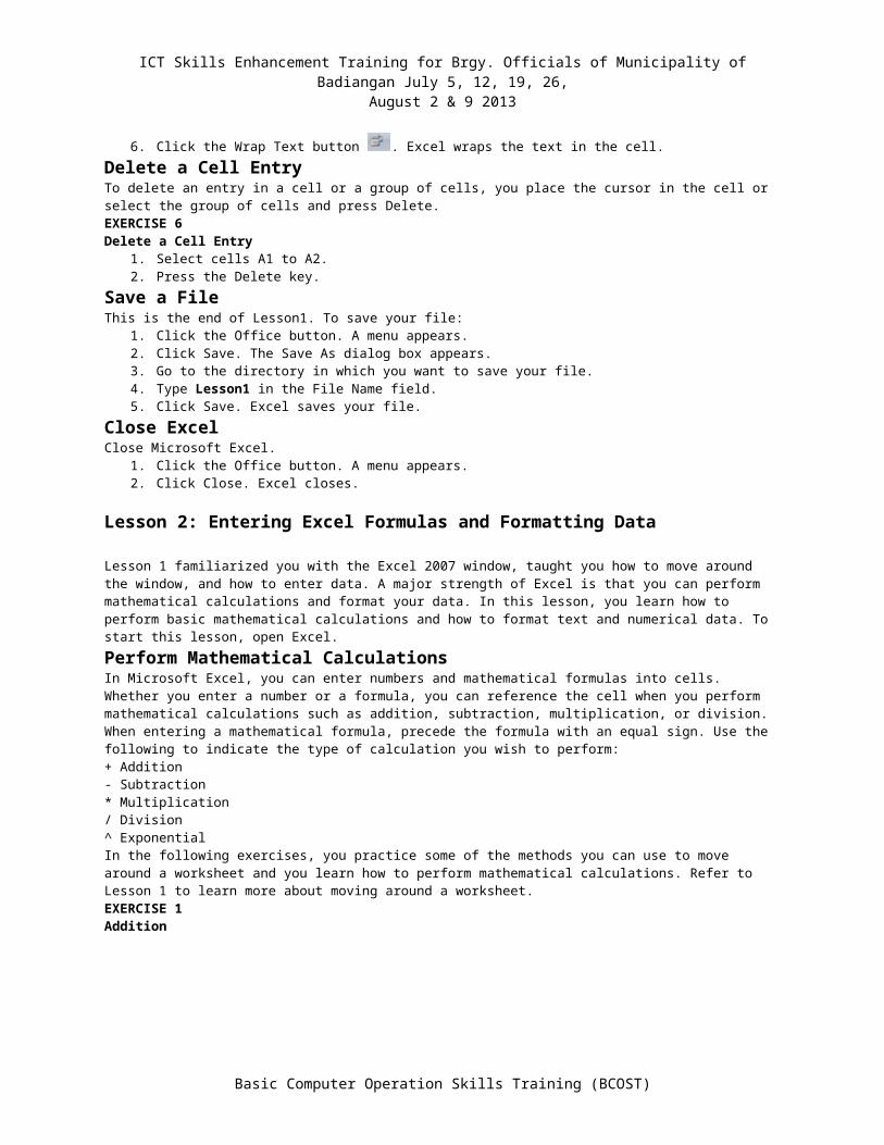
1. Type Add in cell A1.2. Press Enter. Excel moves down one cell.3. Type 1 in cell A2.4. Press Enter. Excel moves down one cell.5. Type 1 in cell A3.6. Press Enter. Excel moves down one cell.7. Type =A2+A3 in cell A4.8. Click the check mark on the Formula bar. Excel adds cell A1 to cell A2 and displays the result in cell A4. The
formula displays on the Formula bar.Note: Clicking the check mark on the Formula bar is similar to pressing Enter. Excel records your entry but does not move to the next cell.Subtraction
1. Press F5. The Go To dialog box appears.2. Type B1 in the Reference field.3. Press Enter. Excel moves to cell B1.
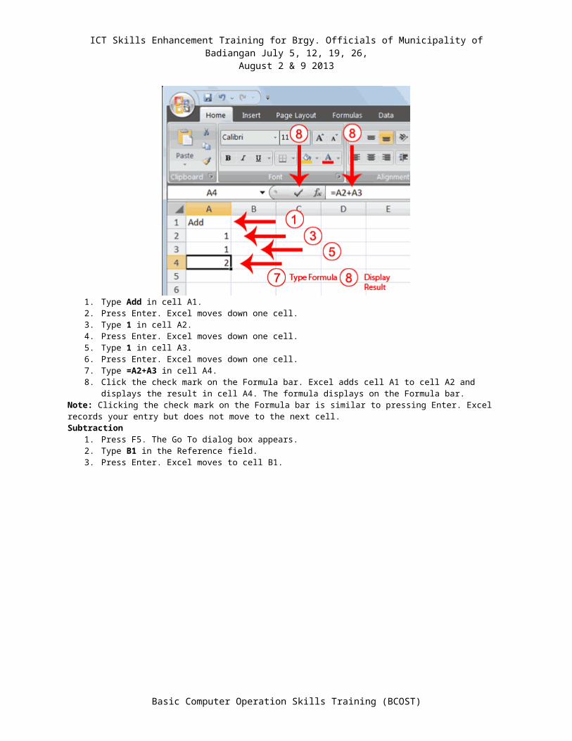
4. Type Subtract.5. Press Enter. Excel moves down one cell.6. Type 6 in cell B2.
Basic Computer Operation Skills Training (BCOST)
ICT Skills Enhancement Training for Brgy. Officials of Municipality of Badiangan July 5, 12, 19, 26,
August 2 & 9 2013
7. Press Enter. Excel moves down one cell.8. Type 3 in cell B3.9. Press Enter. Excel moves down one cell.10. Type =B2-B3 in cell B4.11. Click the check mark on the Formula bar. Excel subtracts cell B3 from cell B2 and the result displays in cell
B4. The formula displays on the Formula bar.Multiplication
1. Hold down the Ctrl key while you press "g" (Ctrl+g). The Go To dialog box appears.2. Type C1 in the Reference field.3. Press Enter. Excel moves to cell C14. Type Multiply.5. Press Enter. Excel moves down one cell.6. Type 2 in cell C2.7. Press Enter. Excel moves down one cell.8. Type 3 in cell C3.9. Press Enter. Excel moves down one cell.10. Type =C2*C3 in cell C4.11. Click the check mark on the Formula bar. Excel multiplies C1 by cell C2 and displays the result in cell C3.
The formula displays on the Formula bar.Division
1. Press F5.2. Type D1 in the Reference field.3. Press Enter. Excel moves to cell D1.4. Type Divide.5. Press Enter. Excel moves down one cell.6. Type 6 in cell D2.7. Press Enter. Excel moves down one cell.8. Type 3 in cell D3.9. Press Enter. Excel moves down one cell.10. Type =D2/D3 in cell D4.11. Click the check mark on the Formula bar. Excel divides cell D2 by cell D3 and displays the result in cell D4.
The formula displays on the Formula bar.When creating formulas, you can reference cells and include numbers. All of the following formulas are valid:=A2/B2=A1+12-B3=A2*B2+12=24+53
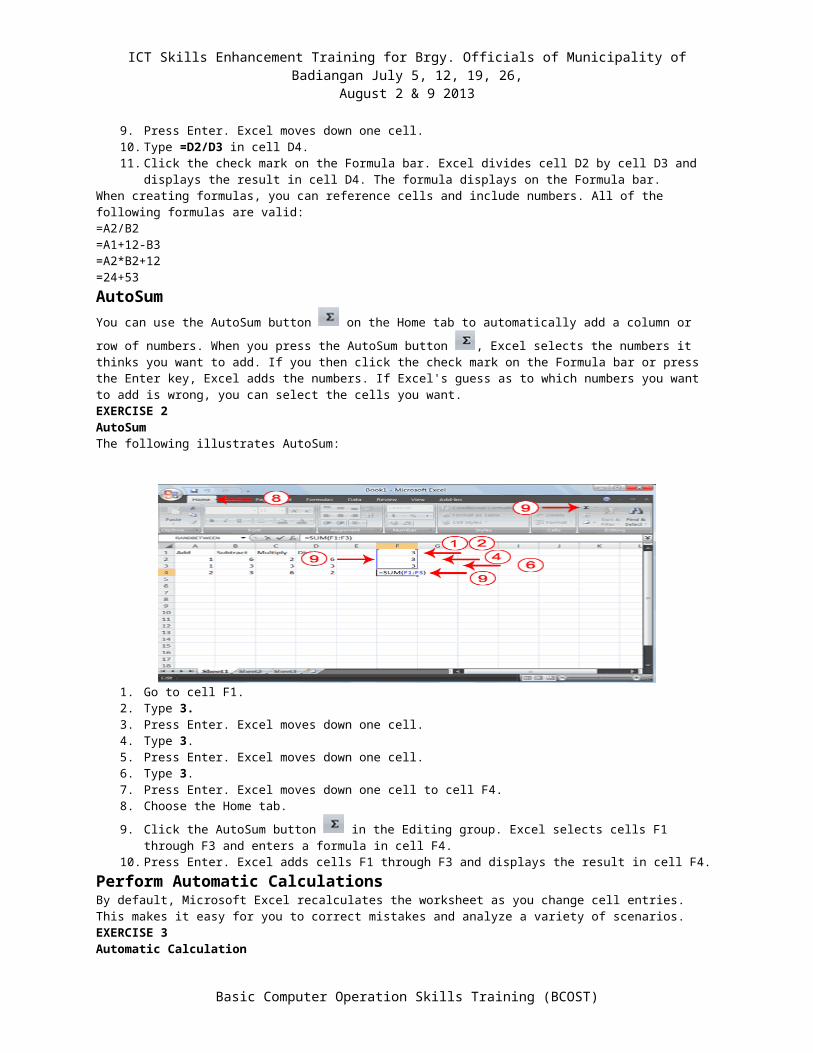
AutoSum
You can use the AutoSum button on the Home tab to automatically add a column or row of numbers. When you
press the AutoSum button , Excel selects the numbers it thinks you want to add. If you then click the check mark on the Formula bar or press the Enter key, Excel adds the numbers. If Excel's guess as to which numbers you want to add is wrong, you can select the cells you want.EXERCISE 2AutoSumThe following illustrates AutoSum:
Basic Computer Operation Skills Training (BCOST)
ICT Skills Enhancement Training for Brgy. Officials of Municipality of Badiangan July 5, 12, 19, 26,
August 2 & 9 2013
1. Go to cell F1.2. Type 3.3. Press Enter. Excel moves down one cell.4. Type 3.5. Press Enter. Excel moves down one cell.6. Type 3.7. Press Enter. Excel moves down one cell to cell F4.8. Choose the Home tab.
9. Click the AutoSum button in the Editing group. Excel selects cells F1 through F3 and enters a formula in cell F4.
10. Press Enter. Excel adds cells F1 through F3 and displays the result in cell F4.
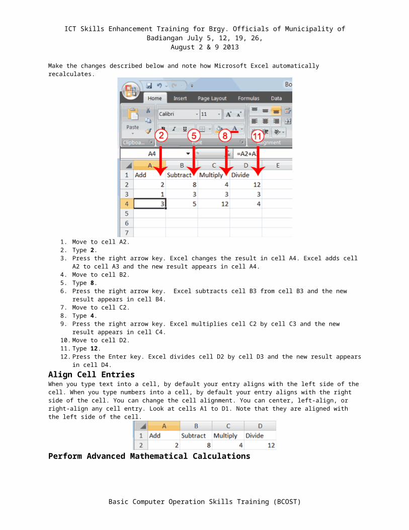
Perform Automatic CalculationsBy default, Microsoft Excel recalculates the worksheet as you change cell entries. This makes it easy for you to correct mistakes and analyze a variety of scenarios.EXERCISE 3Automatic CalculationMake the changes described below and note how Microsoft Excel automatically recalculates.
1. Move to cell A2.2. Type 2.3. Press the right arrow key. Excel changes the result in cell A4. Excel adds cell A2 to cell A3 and the new
result appears in cell A4.4. Move to cell B2.
Basic Computer Operation Skills Training (BCOST)
ICT Skills Enhancement Training for Brgy. Officials of Municipality of Badiangan July 5, 12, 19, 26,
August 2 & 9 2013
5. Type 8.6. Press the right arrow key. Excel subtracts cell B3 from cell B3 and the new result appears in cell B4.7. Move to cell C2.8. Type 4.9. Press the right arrow key. Excel multiplies cell C2 by cell C3 and the new result appears in cell C4.10. Move to cell D2.11. Type 12.12. Press the Enter key. Excel divides cell D2 by cell D3 and the new result appears in cell D4.
Align Cell EntriesWhen you type text into a cell, by default your entry aligns with the left side of the cell. When you type numbers into a cell, by default your entry aligns with the right side of the cell. You can change the cell alignment. You can center, left-align, or right-align any cell entry. Look at cells A1 to D1. Note that they are aligned with the left side of the cell.
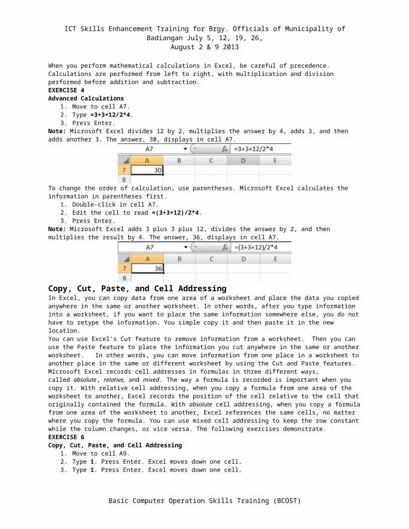
Perform Advanced Mathematical CalculationsWhen you perform mathematical calculations in Excel, be careful of precedence. Calculations are performed from left to right, with multiplication and division performed before addition and subtraction.EXERCISE 4Advanced Calculations
1. Move to cell A7.2. Type =3+3+12/2*4.3. Press Enter.
Note: Microsoft Excel divides 12 by 2, multiplies the answer by 4, adds 3, and then adds another 3. The answer, 30, displays in cell A7.
To change the order of calculation, use parentheses. Microsoft Excel calculates the information in parentheses first.1. Double-click in cell A7.2. Edit the cell to read =(3+3+12)/2*4.3. Press Enter.
Note: Microsoft Excel adds 3 plus 3 plus 12, divides the answer by 2, and then multiplies the result by 4. The answer, 36, displays in cell A7.
Copy, Cut, Paste, and Cell AddressingIn Excel, you can copy data from one area of a worksheet and place the data you copied anywhere in the same or another worksheet. In other words, after you type information into a worksheet, if you want to place the same information somewhere else, you do not have to retype the information. You simple copy it and then paste it in the new location.You can use Excel's Cut feature to remove information from a worksheet. Then you can use the Paste feature to place the information you cut anywhere in the same or another worksheet. In other words, you can move information from one place in a worksheet to another place in the same or different worksheet by using the Cut and Paste features.Microsoft Excel records cell addresses in formulas in three different ways, called absolute, relative, and mixed. The way a formula is recorded is important when you copy it. With relative cell addressing, when you copy a formula from one area of the worksheet to another, Excel records the position of the cell relative to the cell that originally contained the formula. With absolute cell addressing, when you copy a formula from one area of the worksheet to another, Excel references the same cells, no matter where you copy the formula. You can use mixed cell addressing to keep the row constant while the column changes, or vice versa. The following exercises demonstrate.EXERCISE 6
Basic Computer Operation Skills Training (BCOST)
ICT Skills Enhancement Training for Brgy. Officials of Municipality of Badiangan July 5, 12, 19, 26,
August 2 & 9 2013
Copy, Cut, Paste, and Cell Addressing1. Move to cell A9.2. Type 1. Press Enter. Excel moves down one cell.3. Type 1. Press Enter. Excel moves down one cell.4. Type 1. Press Enter. Excel moves down one cell.5. Move to cell B9.6. Type 2. Press Enter. Excel moves down one cell.7. Type 2. Press Enter. Excel moves down one cell.8. Type 2. Press Enter. Excel moves down one cell.
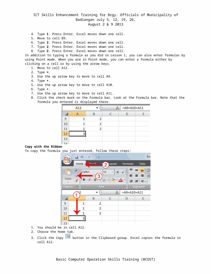
In addition to typing a formula as you did in Lesson 1, you can also enter formulas by using Point mode. When you are in Point mode, you can enter a formula either by clicking on a cell or by using the arrow keys.
1. Move to cell A12.2. Type =.3. Use the up arrow key to move to cell A9.4. Type +.5. Use the up arrow key to move to cell A10.6. Type +.7. Use the up arrow key to move to cell A11.8. Click the check mark on the Formula bar. Look at the Formula bar. Note that the formula you entered is
displayed there.
Copy with the RibbonTo copy the formula you just entered, follow these steps:
1. You should be in cell A12.2. Choose the Home tab.
3. Click the Copy button in the Clipboard group. Excel copies the formula in cell A12.
Basic Computer Operation Skills Training (BCOST)
ICT Skills Enhancement Training for Brgy. Officials of Municipality of Badiangan July 5, 12, 19, 26,
August 2 & 9 2013
4. Press the right arrow key once to move to cell B12.
5. Click the Paste button in the Clipboard group. Excel pastes the formula in cell A12 into cell B12.6. Press the Esc key to exit the Copy mode.
Compare the formula in cell A12 with the formula in cell B12 (while in the respective cell, look at the Formula bar). The formulas are the same except that the formula in cell A12 sums the entries in column A and the formula in cell B12 sums the entries in column B. The formula was copied in a relative fashion.Before proceeding with the next part of the exercise, you must copy the information in cells A7 to B9 to cells C7 to D9. This time you will copy by using the Mini toolbar.Copy with the Mini Toolbar
1. Select cells A9 to B11. Move to cell A9. Press the Shift key. While holding down the Shift key, press the down arrow key twice. Press the right arrow key once. Excel highlights A9 to B11.
2. Right-click. A context menu and a Mini toolbar appear.3. Click Copy, which is located on the context menu. Excel copies the information in cells A9 to B11.
Basic Computer Operation Skills Training (BCOST)
ICT Skills Enhancement Training for Brgy. Officials of Municipality of Badiangan July 5, 12, 19, 26,
August 2 & 9 2013
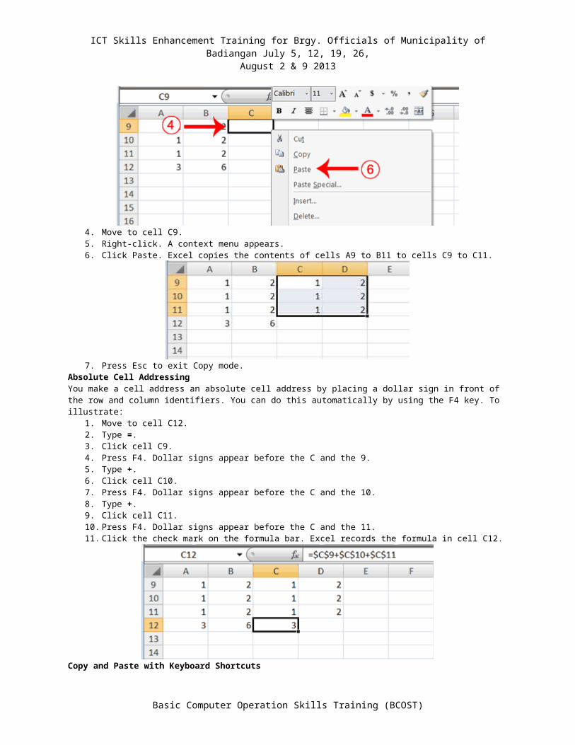
4. Move to cell C9.5. Right-click. A context menu appears.6. Click Paste. Excel copies the contents of cells A9 to B11 to cells C9 to C11.
7. Press Esc to exit Copy mode.Absolute Cell AddressingYou make a cell address an absolute cell address by placing a dollar sign in front of the row and column identifiers. You can do this automatically by using the F4 key. To illustrate:
1. Move to cell C12.2. Type =.3. Click cell C9.4. Press F4. Dollar signs appear before the C and the 9.5. Type +.6. Click cell C10.7. Press F4. Dollar signs appear before the C and the 10.8. Type +.9. Click cell C11.10. Press F4. Dollar signs appear before the C and the 11.11. Click the check mark on the formula bar. Excel records the formula in cell C12.
Copy and Paste with Keyboard ShortcutsKeyboard shortcuts are key combinations that enable you to perform tasks by using the keyboard. Generally, you press and hold down a key while pressing a letter. For example, Ctrl+c means you should press and hold down the Ctrl key while pressing "c." This tutorial notates key combinations as follows:Press Ctrl+c.Now copy the formula from C12 to D12. This time, copy by using keyboard shortcuts.
1. Move to cell C12.
Basic Computer Operation Skills Training (BCOST)

ICT Skills Enhancement Training for Brgy. Officials of Municipality of Badiangan July 5, 12, 19, 26,
August 2 & 9 2013
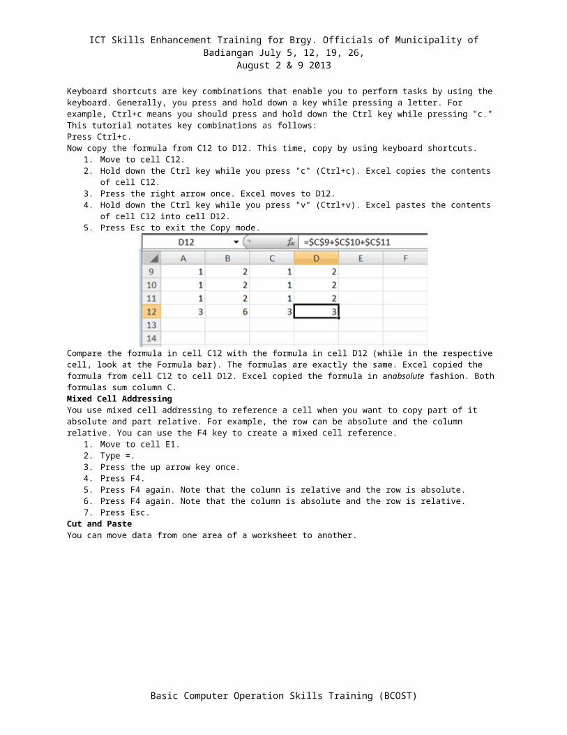
2. Hold down the Ctrl key while you press "c" (Ctrl+c). Excel copies the contents of cell C12.3. Press the right arrow once. Excel moves to D12.4. Hold down the Ctrl key while you press "v" (Ctrl+v). Excel pastes the contents of cell C12 into cell D12.5. Press Esc to exit the Copy mode.
Compare the formula in cell C12 with the formula in cell D12 (while in the respective cell, look at the Formula bar). The formulas are exactly the same. Excel copied the formula from cell C12 to cell D12. Excel copied the formula in anabsolute fashion. Both formulas sum column C.Mixed Cell AddressingYou use mixed cell addressing to reference a cell when you want to copy part of it absolute and part relative. For example, the row can be absolute and the column relative. You can use the F4 key to create a mixed cell reference.
1. Move to cell E1.2. Type =.3. Press the up arrow key once.4. Press F4.5. Press F4 again. Note that the column is relative and the row is absolute.6. Press F4 again. Note that the column is absolute and the row is relative.7. Press Esc.
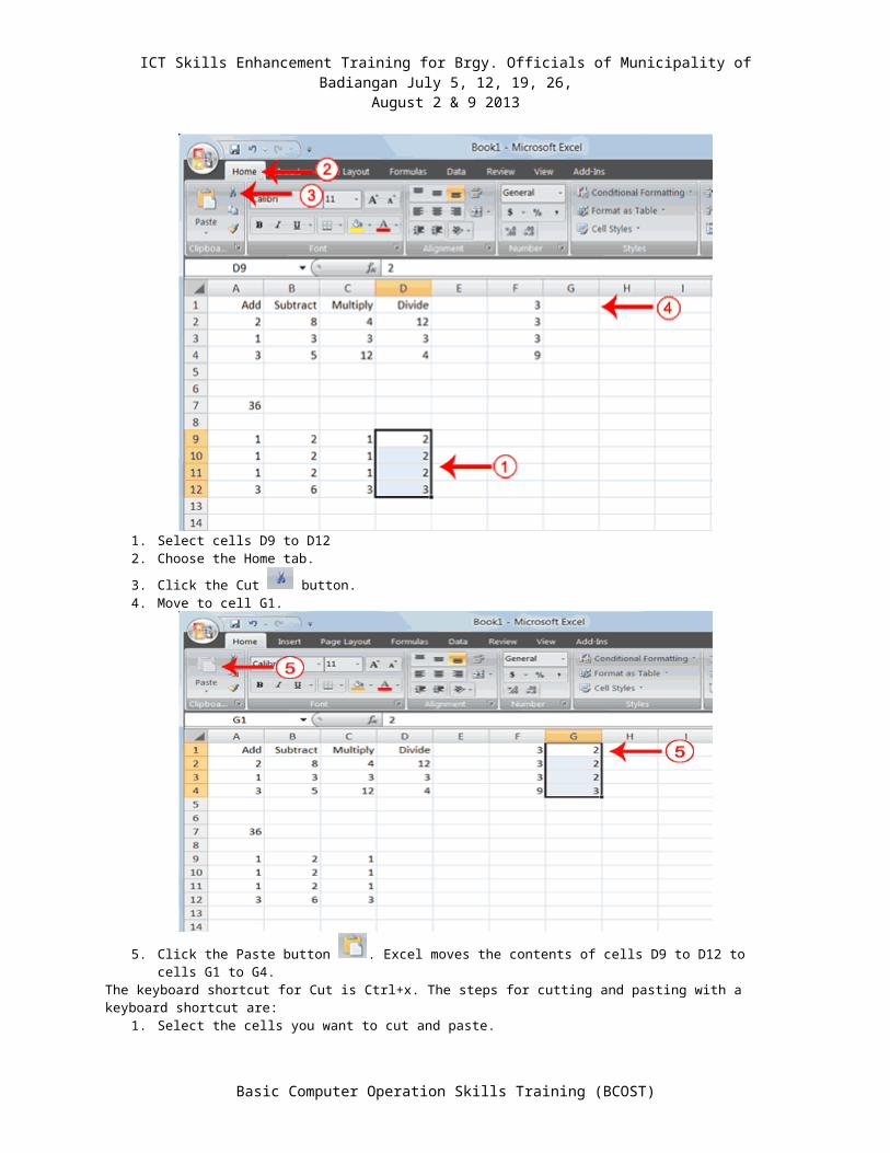
Cut and PasteYou can move data from one area of a worksheet to another.
1. Select cells D9 to D122. Choose the Home tab.
3. Click the Cut button.
Basic Computer Operation Skills Training (BCOST)
ICT Skills Enhancement Training for Brgy. Officials of Municipality of Badiangan July 5, 12, 19, 26,
August 2 & 9 2013
4. Move to cell G1.
5. Click the Paste button . Excel moves the contents of cells D9 to D12 to cells G1 to G4.The keyboard shortcut for Cut is Ctrl+x. The steps for cutting and pasting with a keyboard shortcut are:
1. Select the cells you want to cut and paste.2. Press Ctrl+x.3. Move to the upper-left corner of the block of cells into which you want to paste.4. Press Ctrl+v. Excel cuts and pastes the cells you selected.
Insert and Delete Columns and RowsYou can insert and delete columns and rows. When you delete a column, you delete everything in the column from the top of the worksheet to the bottom of the worksheet. When you delete a row, you delete the entire row from left to right. Inserting a column or row inserts a completely new column or row.EXERCISE 7Insert and Delete Columns and RowsTo delete columns F and G:
Basic Computer Operation Skills Training (BCOST)
ICT Skills Enhancement Training for Brgy. Officials of Municipality of Badiangan July 5, 12, 19, 26,
August 2 & 9 2013
1. Click the column F indicator and drag to column G.2. Click the down arrow next to Delete in the Cells group. A menu appears.3. Click Delete Sheet Columns. Excel deletes the columns you selected.4. Click anywhere on the worksheet to remove your selection.
To delete rows 7 through 12:
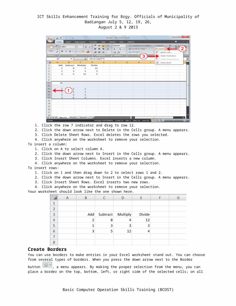
1. Click the row 7 indicator and drag to row 12.2. Click the down arrow next to Delete in the Cells group. A menu appears.3. Click Delete Sheet Rows. Excel deletes the rows you selected.4. Click anywhere on the worksheet to remove your selection.
To insert a column:1. Click on A to select column A.2. Click the down arrow next to Insert in the Cells group. A menu appears.3. Click Insert Sheet Columns. Excel inserts a new column.
Basic Computer Operation Skills Training (BCOST)
ICT Skills Enhancement Training for Brgy. Officials of Municipality of Badiangan July 5, 12, 19, 26,
August 2 & 9 2013
4. Click anywhere on the worksheet to remove your selection.To insert rows:
1. Click on 1 and then drag down to 2 to select rows 1 and 2.2. Click the down arrow next to Insert in the Cells group. A menu appears.3. Click Insert Sheet Rows. Excel inserts two new rows.4. Click anywhere on the worksheet to remove your selection.
Your worksheet should look like the one shown here.
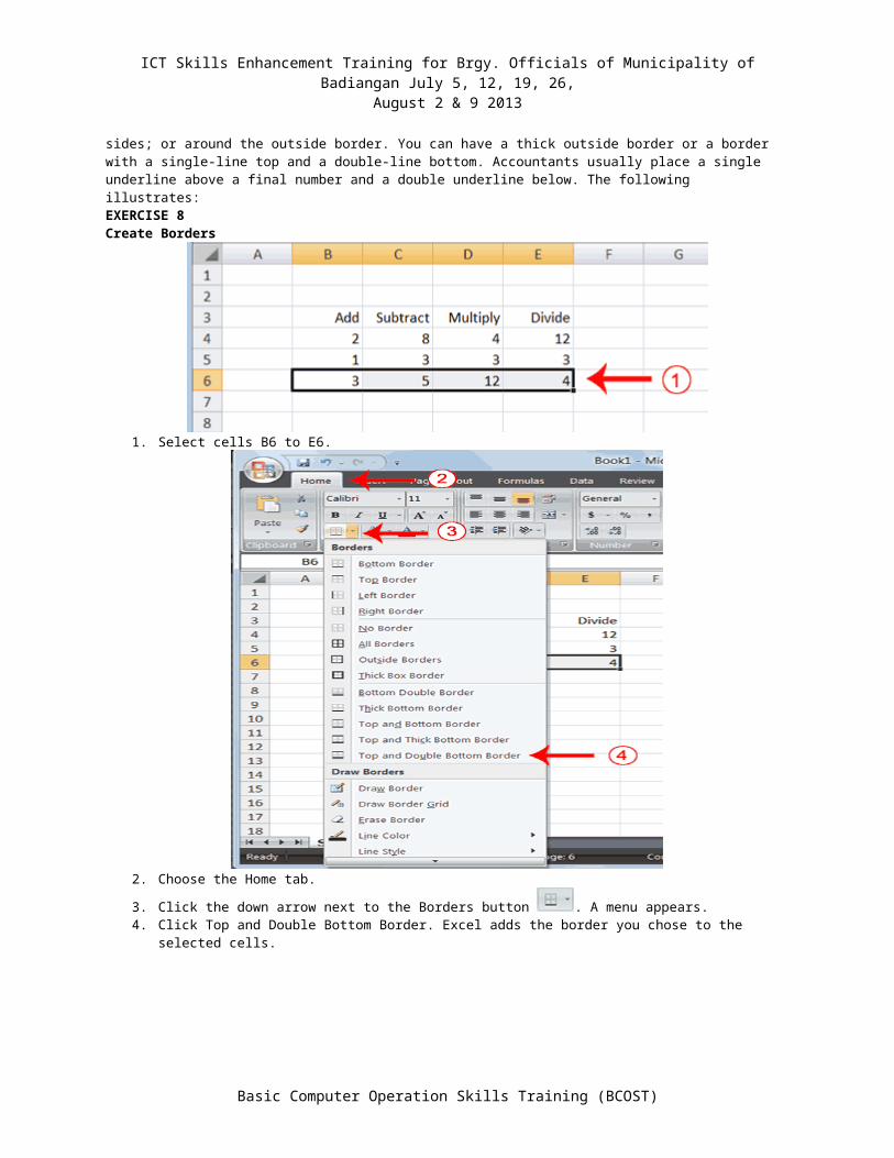
Create BordersYou can use borders to make entries in your Excel worksheet stand out. You can choose from several types of
borders. When you press the down arrow next to the Border button , a menu appears. By making the proper selection from the menu, you can place a border on the top, bottom, left, or right side of the selected cells; on all sides; or around the outside border. You can have a thick outside border or a border with a single-line top and a double-line bottom. Accountants usually place a single underline above a final number and a double underline below. The following illustrates:EXERCISE 8Create Borders
1. Select cells B6 to E6.
Basic Computer Operation Skills Training (BCOST)

ICT Skills Enhancement Training for Brgy. Officials of Municipality of Badiangan July 5, 12, 19, 26,
August 2 & 9 2013
2. Choose the Home tab.
3. Click the down arrow next to the Borders button . A menu appears.4. Click Top and Double Bottom Border. Excel adds the border you chose to the selected cells.
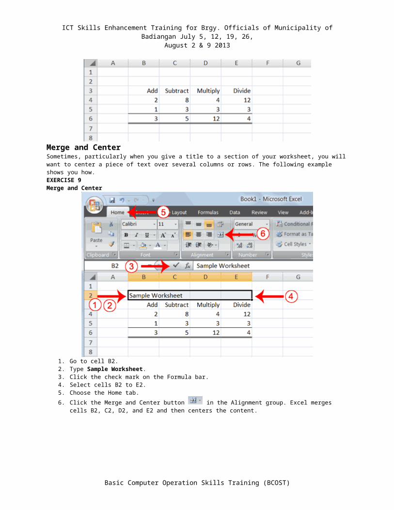
Merge and CenterSometimes, particularly when you give a title to a section of your worksheet, you will want to center a piece of text over several columns or rows. The following example shows you how.EXERCISE 9Merge and Center
Basic Computer Operation Skills Training (BCOST)
ICT Skills Enhancement Training for Brgy. Officials of Municipality of Badiangan July 5, 12, 19, 26,
August 2 & 9 2013
1. Go to cell B2.2. Type Sample Worksheet.3. Click the check mark on the Formula bar.4. Select cells B2 to E2.5. Choose the Home tab.
6. Click the Merge and Center button in the Alignment group. Excel merges cells B2, C2, D2, and E2 and then centers the content.
Note: To unmerge cells:1. Select the cell you want to unmerge.2. Choose the Home tab.
3. Click the down arrow next to the Merge and Center button. A menu appears.4. Click Unmerge Cells. Excel unmerges the cells.
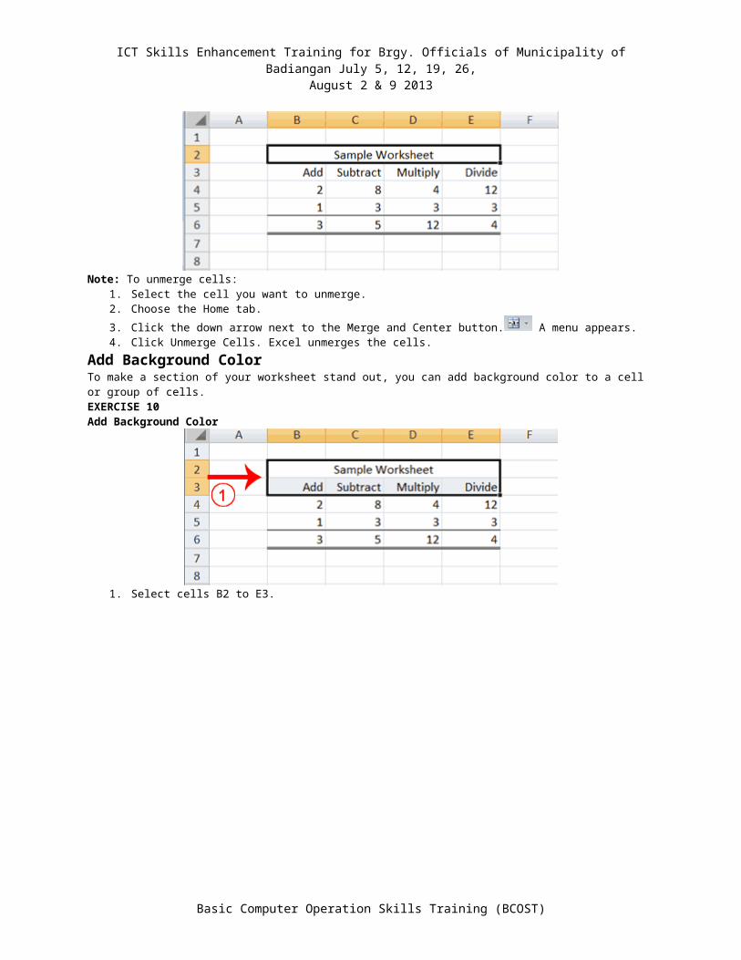
Add Background ColorTo make a section of your worksheet stand out, you can add background color to a cell or group of cells.EXERCISE 10Add Background Color
Basic Computer Operation Skills Training (BCOST)
ICT Skills Enhancement Training for Brgy. Officials of Municipality of Badiangan July 5, 12, 19, 26,
August 2 & 9 2013
1. Select cells B2 to E3.
2. Choose the Home tab.
3. Click the down arrow next to the Fill Color button .4. Click the color dark blue. Excel places a dark blue background in the cells you selected.
Change the Font, Font Size, and Font ColorA font is a set of characters represented in a single typeface. Each character within a font is created by using the same basic style. Excel provides many different fonts from which you can choose. The size of a font is measured in points. There are 72 points to an inch. The number of points assigned to a font is based on the distance from the top
Basic Computer Operation Skills Training (BCOST)
ICT Skills Enhancement Training for Brgy. Officials of Municipality of Badiangan July 5, 12, 19, 26,
August 2 & 9 2013
to the bottom of its longest character. You can change the Font, Font Size, and Font Color of the data you enter into Excel.EXERCISE 11Change the Font
1. Select cells B2 to E3.
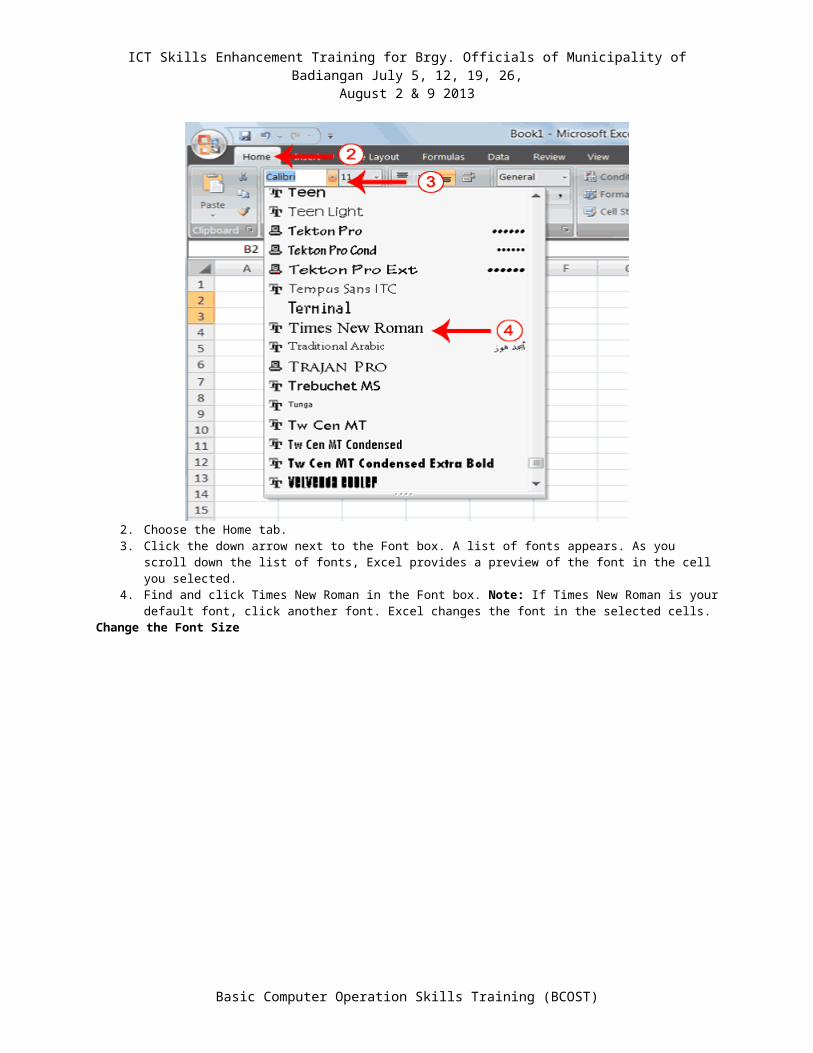
2. Choose the Home tab.3. Click the down arrow next to the Font box. A list of fonts appears. As you scroll down the list of fonts, Excel
provides a preview of the font in the cell you selected.4. Find and click Times New Roman in the Font box. Note: If Times New Roman is your default font, click
another font. Excel changes the font in the selected cells.Change the Font Size
Basic Computer Operation Skills Training (BCOST)
ICT Skills Enhancement Training for Brgy. Officials of Municipality of Badiangan July 5, 12, 19, 26,
August 2 & 9 2013
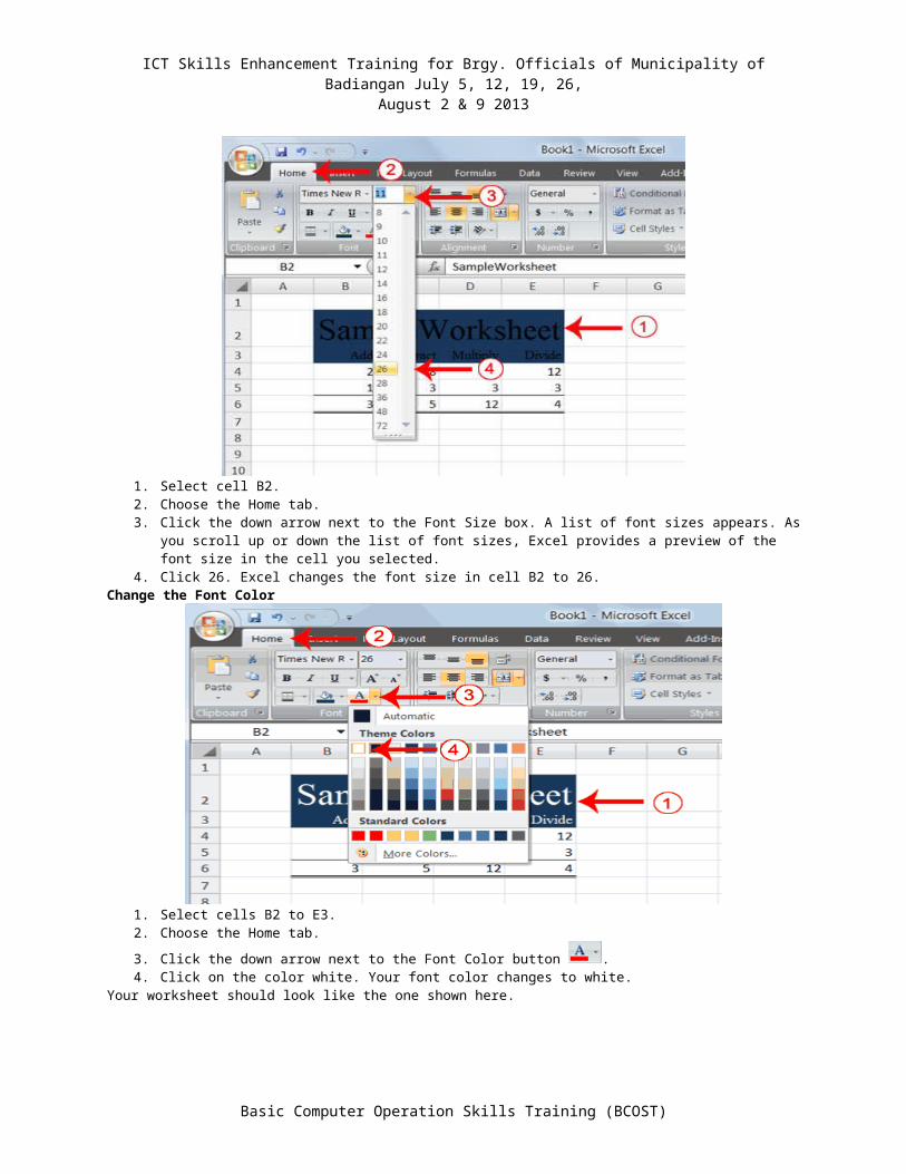
1. Select cell B2.2. Choose the Home tab.3. Click the down arrow next to the Font Size box. A list of font sizes appears. As you scroll up or down the list
of font sizes, Excel provides a preview of the font size in the cell you selected.4. Click 26. Excel changes the font size in cell B2 to 26.
Change the Font Color
1. Select cells B2 to E3.2. Choose the Home tab.
3. Click the down arrow next to the Font Color button .4. Click on the color white. Your font color changes to white.
Your worksheet should look like the one shown here.
Basic Computer Operation Skills Training (BCOST)

ICT Skills Enhancement Training for Brgy. Officials of Municipality of Badiangan July 5, 12, 19, 26,
August 2 & 9 2013
Move to a New WorksheetIn Microsoft Excel, each workbook is made up of several worksheets. Each worksheet has a tab. By default, a workbook has three sheets and they are named sequentially, starting with Sheet1. The name of the worksheet appears on the tab. Before moving to the next topic, move to a new worksheet. The exercise that follows shows you how.EXERCISE 12Move to a New Worksheet
Click Sheet2 in the lower-left corner of the screen. Excel moves to Sheet2.
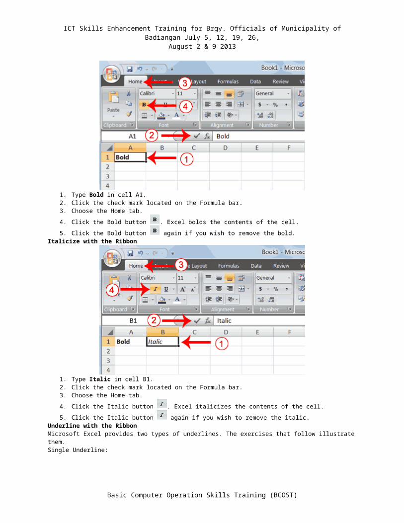
Bold, Italicize, and UnderlineWhen creating an Excel worksheet, you may want to emphasize the contents of cells by bolding, italicizing, and/or underlining. You can easily bold, italicize, or underline text with Microsoft Excel. You can also combine these features—in other words, you can bold, italicize, and underline a single piece of text.In the exercises that follow, you will learn different methods you can use to bold, italicize, and underline.EXERCISE 13Bold with the Ribbon
1. Type Bold in cell A1.2. Click the check mark located on the Formula bar.3. Choose the Home tab.
Basic Computer Operation Skills Training (BCOST)
ICT Skills Enhancement Training for Brgy. Officials of Municipality of Badiangan July 5, 12, 19, 26,
August 2 & 9 2013
4. Click the Bold button . Excel bolds the contents of the cell.
5. Click the Bold button again if you wish to remove the bold.Italicize with the Ribbon
1. Type Italic in cell B1.2. Click the check mark located on the Formula bar.3. Choose the Home tab.
4. Click the Italic button . Excel italicizes the contents of the cell.
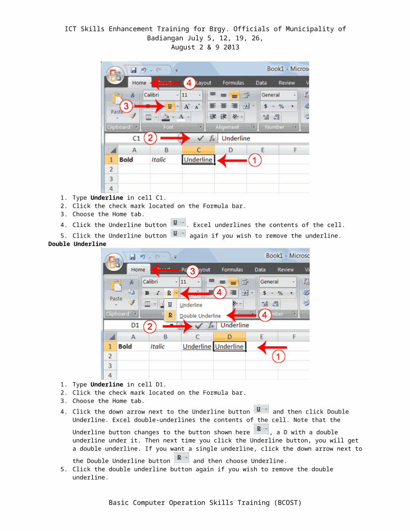
5. Click the Italic button again if you wish to remove the italic.Underline with the RibbonMicrosoft Excel provides two types of underlines. The exercises that follow illustrate them.Single Underline:
1. Type Underline in cell C1.2. Click the check mark located on the Formula bar.3. Choose the Home tab.
4. Click the Underline button . Excel underlines the contents of the cell.
5. Click the Underline button again if you wish to remove the underline.Double Underline
Basic Computer Operation Skills Training (BCOST)
ICT Skills Enhancement Training for Brgy. Officials of Municipality of Badiangan July 5, 12, 19, 26,
August 2 & 9 2013
1. Type Underline in cell D1.2. Click the check mark located on the Formula bar.3. Choose the Home tab.
4. Click the down arrow next to the Underline button and then click Double Underline. Excel double-
underlines the contents of the cell. Note that the Underline button changes to the button shown here , a D with a double underline under it. Then next time you click the Underline button, you will get a double
underline. If you want a single underline, click the down arrow next to the Double Underline button and then choose Underline.
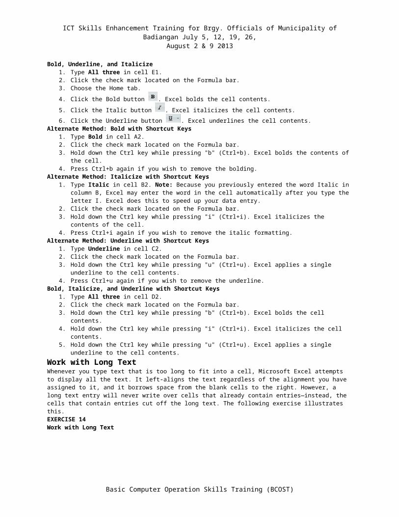
5. Click the double underline button again if you wish to remove the double underline.Bold, Underline, and Italicize
1. Type All three in cell E1.2. Click the check mark located on the Formula bar.3. Choose the Home tab.
4. Click the Bold button . Excel bolds the cell contents.
5. Click the Italic button . Excel italicizes the cell contents.
6. Click the Underline button . Excel underlines the cell contents.Alternate Method: Bold with Shortcut Keys
1. Type Bold in cell A2.2. Click the check mark located on the Formula bar.3. Hold down the Ctrl key while pressing "b" (Ctrl+b). Excel bolds the contents of the cell.4. Press Ctrl+b again if you wish to remove the bolding.
Alternate Method: Italicize with Shortcut Keys1. Type Italic in cell B2. Note: Because you previously entered the word Italic in column B, Excel may enter
the word in the cell automatically after you type the letter I. Excel does this to speed up your data entry.2. Click the check mark located on the Formula bar.3. Hold down the Ctrl key while pressing "i" (Ctrl+i). Excel italicizes the contents of the cell.4. Press Ctrl+i again if you wish to remove the italic formatting.
Alternate Method: Underline with Shortcut Keys1. Type Underline in cell C2.2. Click the check mark located on the Formula bar.3. Hold down the Ctrl key while pressing "u" (Ctrl+u). Excel applies a single underline to the cell contents.4. Press Ctrl+u again if you wish to remove the underline.
Bold, Italicize, and Underline with Shortcut Keys1. Type All three in cell D2.2. Click the check mark located on the Formula bar.3. Hold down the Ctrl key while pressing "b" (Ctrl+b). Excel bolds the cell contents.4. Hold down the Ctrl key while pressing "i" (Ctrl+i). Excel italicizes the cell contents.5. Hold down the Ctrl key while pressing "u" (Ctrl+u). Excel applies a single underline to the cell contents.
Basic Computer Operation Skills Training (BCOST)

ICT Skills Enhancement Training for Brgy. Officials of Municipality of Badiangan July 5, 12, 19, 26,
August 2 & 9 2013
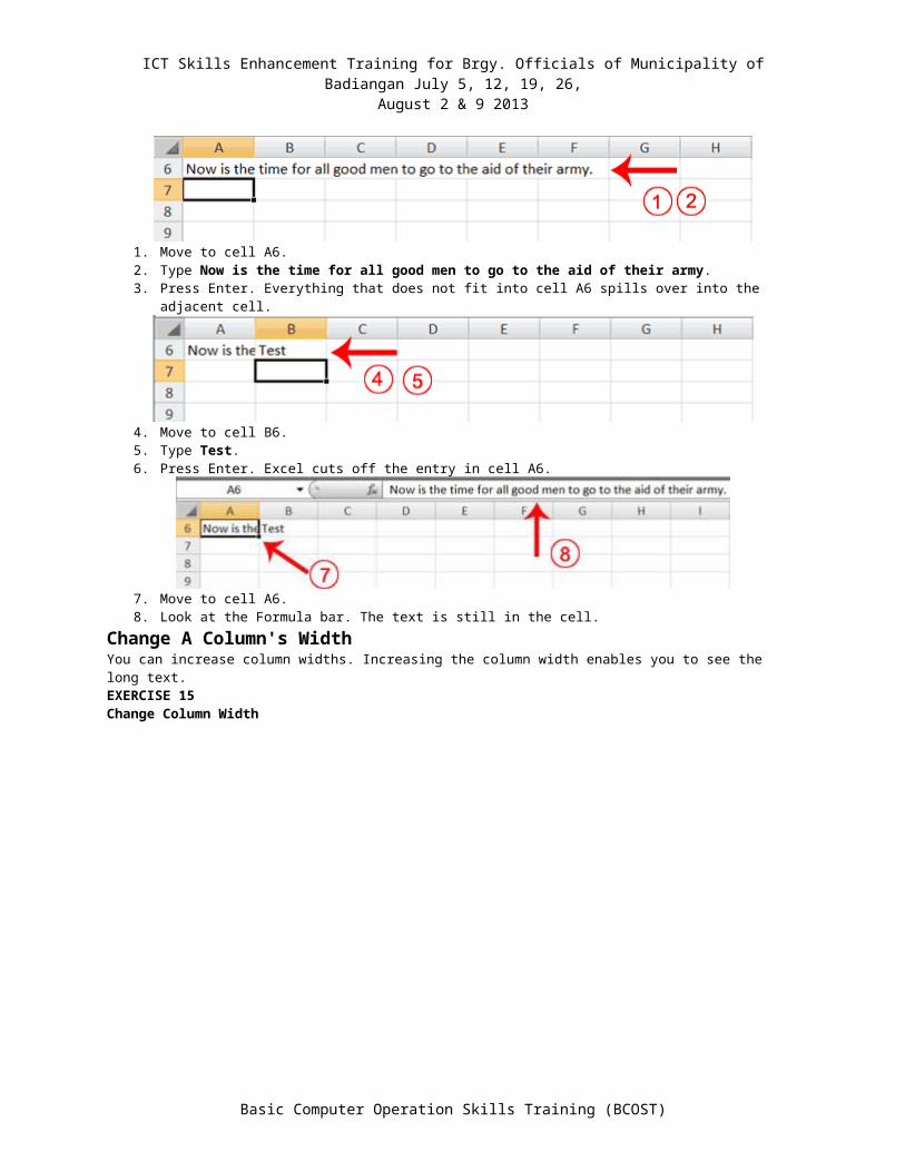
Work with Long TextWhenever you type text that is too long to fit into a cell, Microsoft Excel attempts to display all the text. It left-aligns the text regardless of the alignment you have assigned to it, and it borrows space from the blank cells to the right. However, a long text entry will never write over cells that already contain entries—instead, the cells that contain entries cut off the long text. The following exercise illustrates this.EXERCISE 14Work with Long Text
1. Move to cell A6.2. Type Now is the time for all good men to go to the aid of their army.3. Press Enter. Everything that does not fit into cell A6 spills over into the adjacent cell.
4. Move to cell B6.5. Type Test.6. Press Enter. Excel cuts off the entry in cell A6.
7. Move to cell A6.8. Look at the Formula bar. The text is still in the cell.
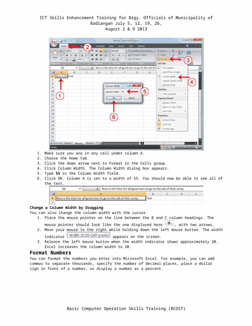
Change A Column's WidthYou can increase column widths. Increasing the column width enables you to see the long text.EXERCISE 15Change Column Width
Basic Computer Operation Skills Training (BCOST)
ICT Skills Enhancement Training for Brgy. Officials of Municipality of Badiangan July 5, 12, 19, 26,
August 2 & 9 2013
1. Make sure you are in any cell under column A.2. Choose the Home tab.3. Click the down arrow next to Format in the Cells group.4. Click Column Width. The Column Width dialog box appears.5. Type 55 in the Column Width field.6. Click OK. Column A is set to a width of 55. You should now be able to see all of the text.
Change a Column Width by DraggingYou can also change the column width with the cursor.
1. Place the mouse pointer on the line between the B and C column headings. The mouse pointer should look
like the one displayed here , with two arrows.2. Move your mouse to the right while holding down the left mouse button. The width
indicator appears on the screen.3. Release the left mouse button when the width indicator shows approximately 20. Excel increases the
column width to 20.
Format NumbersYou can format the numbers you enter into Microsoft Excel. For example, you can add commas to separate thousands, specify the number of decimal places, place a dollar sign in front of a number, or display a number as a percent.
EXERCISE 16Format Numbers
Basic Computer Operation Skills Training (BCOST)
ICT Skills Enhancement Training for Brgy. Officials of Municipality of Badiangan July 5, 12, 19, 26,
August 2 & 9 2013
1. Move to cell B8.2. Type 1234567.3. Click the check mark on the Formula bar.
4. Choose the Home tab.5. Click the down arrow next to the Number Format box. A menu appears.6. Click Number. Excel adds two decimal places to the number you typed.
Basic Computer Operation Skills Training (BCOST)
ICT Skills Enhancement Training for Brgy. Officials of Municipality of Badiangan July 5, 12, 19, 26,
August 2 & 9 2013
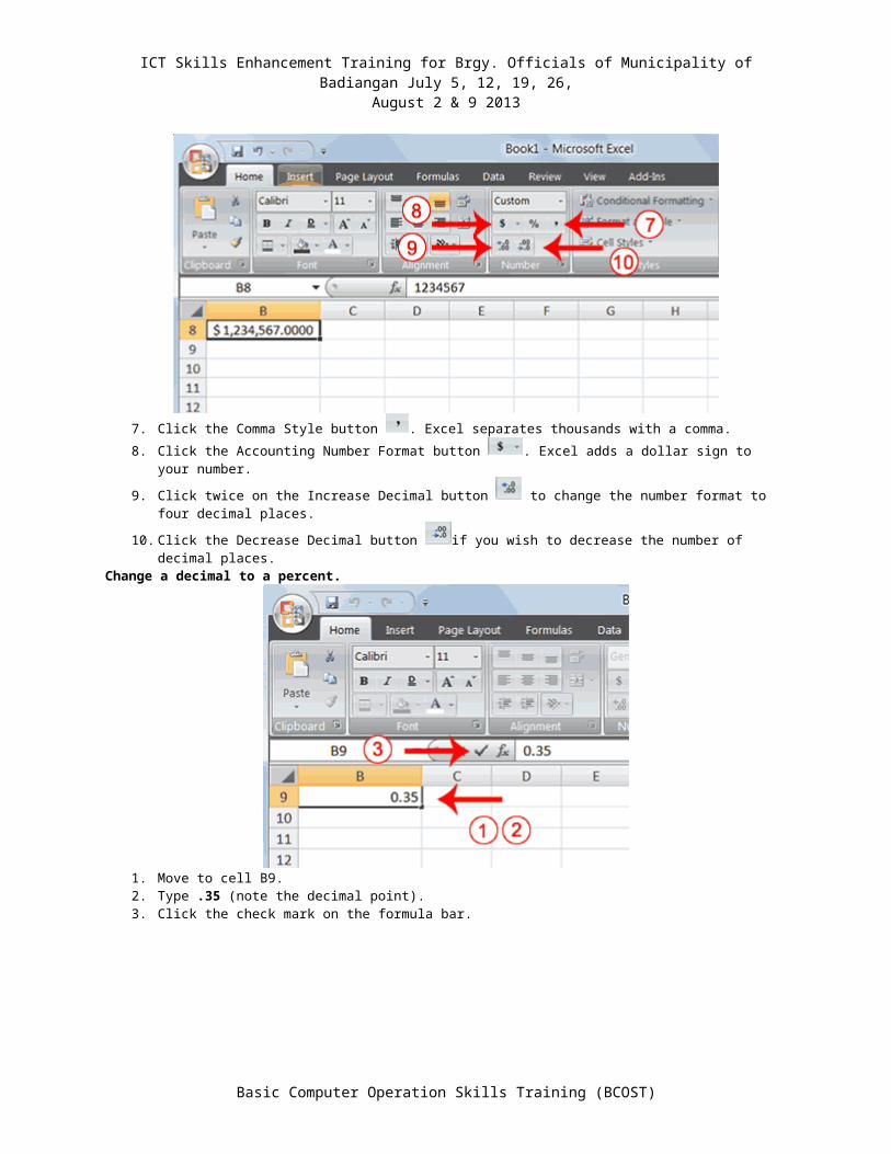
7. Click the Comma Style button . Excel separates thousands with a comma.
8. Click the Accounting Number Format button . Excel adds a dollar sign to your number.
9. Click twice on the Increase Decimal button to change the number format to four decimal places.
10. Click the Decrease Decimal button if you wish to decrease the number of decimal places.Change a decimal to a percent.
1. Move to cell B9.2. Type .35 (note the decimal point).3. Click the check mark on the formula bar.
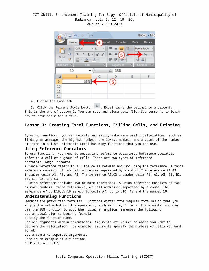
4. Choose the Home tab.
5. Click the Percent Style button . Excel turns the decimal to a percent.This is the end of Lesson 2. You can save and close your file. See Lesson 1 to learn how to save and close a file.
Lesson 3: Creating Excel Functions, Filling Cells, and Printing
By using functions, you can quickly and easily make many useful calculations, such as finding an average, the highest number, the lowest number, and a count of the number of items in a list. Microsoft Excel has many functions that you can use.
Using Reference Operators
Basic Computer Operation Skills Training (BCOST)
ICT Skills Enhancement Training for Brgy. Officials of Municipality of Badiangan July 5, 12, 19, 26,
August 2 & 9 2013
To use functions, you need to understand reference operators. Reference operators refer to a cell or a group of cells. There are two types of reference operators: range andunion.A range reference refers to all the cells between and including the reference. A range reference consists of two cell addresses separated by a colon. The reference A1:A3 includes cells A1, A2, and A3. The reference A1:C3 includes cells A1, A2, A3, B1, B2, B3, C1, C2, and C3.A union reference includes two or more references. A union reference consists of two or more numbers, range references, or cell addresses separated by a comma. The reference A7,B8:B10,C9,10 refers to cells A7, B8 to B10, C9 and the number 10.
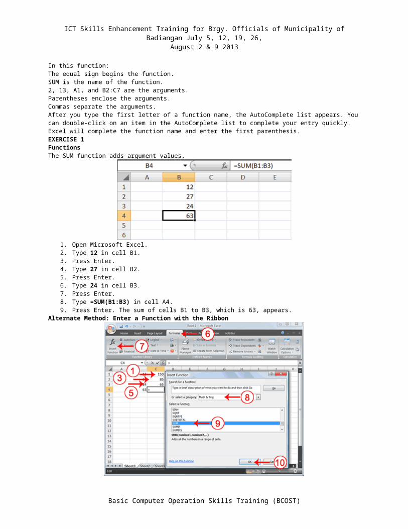
Understanding FunctionsFunctions are prewritten formulas. Functions differ from regular formulas in that you supply the value but not the operators, such as +, -, *, or /. For example, you can use the SUM function to add. When using a function, remember the following:Use an equal sign to begin a formula.Specify the function name.Enclose arguments within parentheses. Arguments are values on which you want to perform the calculation. For example, arguments specify the numbers or cells you want to add.Use a comma to separate arguments.Here is an example of a function:=SUM(2,13,A1,B2:C7)In this function:The equal sign begins the function.SUM is the name of the function.2, 13, A1, and B2:C7 are the arguments.Parentheses enclose the arguments.Commas separate the arguments.After you type the first letter of a function name, the AutoComplete list appears. You can double-click on an item in the AutoComplete list to complete your entry quickly. Excel will complete the function name and enter the first parenthesis.EXERCISE 1FunctionsThe SUM function adds argument values.
1. Open Microsoft Excel.2. Type 12 in cell B1.3. Press Enter.4. Type 27 in cell B2.5. Press Enter.6. Type 24 in cell B3.7. Press Enter.8. Type =SUM(B1:B3) in cell A4.9. Press Enter. The sum of cells B1 to B3, which is 63, appears.
Alternate Method: Enter a Function with the Ribbon
Basic Computer Operation Skills Training (BCOST)
ICT Skills Enhancement Training for Brgy. Officials of Municipality of Badiangan July 5, 12, 19, 26,
August 2 & 9 2013
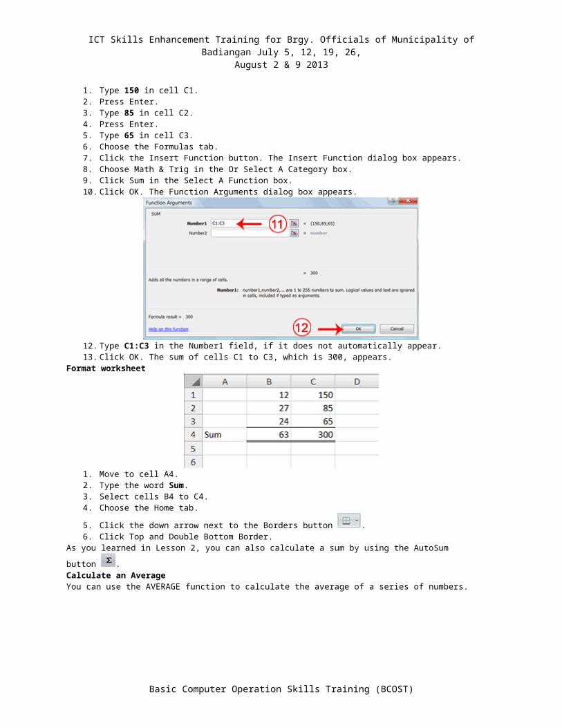
1. Type 150 in cell C1.2. Press Enter.3. Type 85 in cell C2.4. Press Enter.5. Type 65 in cell C3.6. Choose the Formulas tab.7. Click the Insert Function button. The Insert Function dialog box appears.8. Choose Math & Trig in the Or Select A Category box.9. Click Sum in the Select A Function box.10. Click OK. The Function Arguments dialog box appears.
12. Type C1:C3 in the Number1 field, if it does not automatically appear.13. Click OK. The sum of cells C1 to C3, which is 300, appears.
Format worksheet
1. Move to cell A4.
Basic Computer Operation Skills Training (BCOST)

ICT Skills Enhancement Training for Brgy. Officials of Municipality of Badiangan July 5, 12, 19, 26,
August 2 & 9 2013
2. Type the word Sum.3. Select cells B4 to C4.4. Choose the Home tab.
5. Click the down arrow next to the Borders button .6. Click Top and Double Bottom Border.
As you learned in Lesson 2, you can also calculate a sum by using the AutoSum button .Calculate an AverageYou can use the AVERAGE function to calculate the average of a series of numbers.
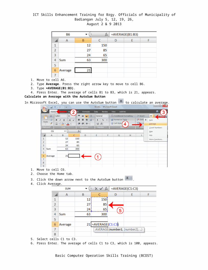
1. Move to cell A6.2. Type Average. Press the right arrow key to move to cell B6.3. Type =AVERAGE(B1:B3).4. Press Enter. The average of cells B1 to B3, which is 21, appears.
Calculate an Average with the AutoSum Button
In Microsoft Excel, you can use the AutoSum button to calculate an average.
1. Move to cell C6.2. Choose the Home tab.
3. Click the down arrow next to the AutoSum button .4. Click Average.
Basic Computer Operation Skills Training (BCOST)
ICT Skills Enhancement Training for Brgy. Officials of Municipality of Badiangan July 5, 12, 19, 26,
August 2 & 9 2013
5. Select cells C1 to C3.6. Press Enter. The average of cells C1 to C3, which is 100, appears.
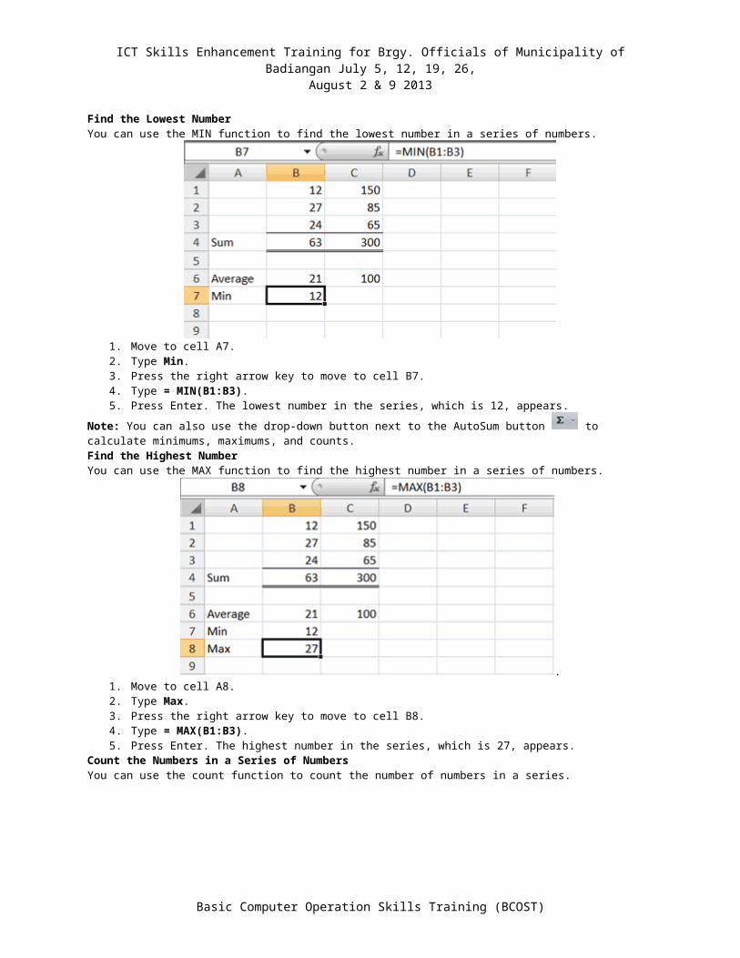
Find the Lowest NumberYou can use the MIN function to find the lowest number in a series of numbers.
1. Move to cell A7.2. Type Min.3. Press the right arrow key to move to cell B7.4. Type = MIN(B1:B3).5. Press Enter. The lowest number in the series, which is 12, appears.
Note: You can also use the drop-down button next to the AutoSum button to calculate minimums, maximums, and counts.Find the Highest NumberYou can use the MAX function to find the highest number in a series of numbers.
.1. Move to cell A8.
Basic Computer Operation Skills Training (BCOST)
ICT Skills Enhancement Training for Brgy. Officials of Municipality of Badiangan July 5, 12, 19, 26,
August 2 & 9 2013
2. Type Max.3. Press the right arrow key to move to cell B8.4. Type = MAX(B1:B3).5. Press Enter. The highest number in the series, which is 27, appears.
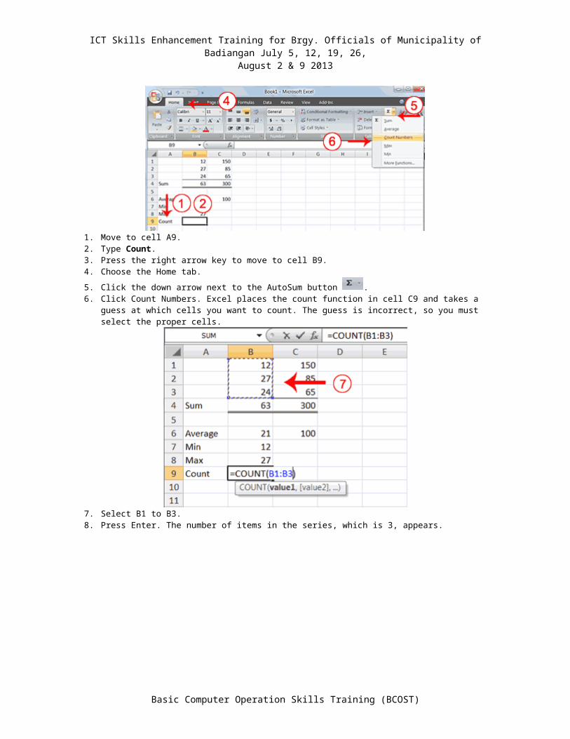
Count the Numbers in a Series of NumbersYou can use the count function to count the number of numbers in a series.
1. Move to cell A9.2. Type Count.3. Press the right arrow key to move to cell B9.4. Choose the Home tab.
5. Click the down arrow next to the AutoSum button .6. Click Count Numbers. Excel places the count function in cell C9 and takes a guess at which cells you want
to count. The guess is incorrect, so you must select the proper cells.
7. Select B1 to B3.8. Press Enter. The number of items in the series, which is 3, appears.
Basic Computer Operation Skills Training (BCOST)
ICT Skills Enhancement Training for Brgy. Officials of Municipality of Badiangan July 5, 12, 19, 26,
August 2 & 9 2013
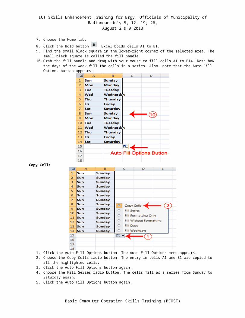
Fill Cells AutomaticallyYou can use Microsoft Excel to fill cells automatically with a series. For example, you can have Excel automatically fill your worksheet with days of the week, months of the year, years, or other types of series.EXERCISE 2Fill Cells AutomaticallyThe following demonstrates filling the days of the week:
1. Click the Sheet2 tab. Excel moves to Sheet2.2. Move to cell A1.3. Type Sun.4. Move to cell B1.5. Type Sunday.6. Select cells A1 to B1.7. Choose the Home tab.
8. Click the Bold button . Excel bolds cells A1 to B1.9. Find the small black square in the lower-right corner of the selected area. The small black square is called
the fill handle.
Basic Computer Operation Skills Training (BCOST)
ICT Skills Enhancement Training for Brgy. Officials of Municipality of Badiangan July 5, 12, 19, 26,
August 2 & 9 2013
10. Grab the fill handle and drag with your mouse to fill cells A1 to B14. Note how the days of the week fill the cells in a series. Also, note that the Auto Fill Options button appears.
Copy Cells
1. Click the Auto Fill Options button. The Auto Fill Options menu appears.2. Choose the Copy Cells radio button. The entry in cells A1 and B1 are copied to all the highlighted cells.3. Click the Auto Fill Options button again.4. Choose the Fill Series radio button. The cells fill as a series from Sunday to Saturday again.5. Click the Auto Fill Options button again.6. Choose the Fill Without Formatting radio button. The cells fill as a series from Sunday to Saturday, but the
entries are not bolded.7. Click the Auto Fill Options button again.8. Choose the Fill Weekdays radio button. The cells fill as a series from Monday to Friday.
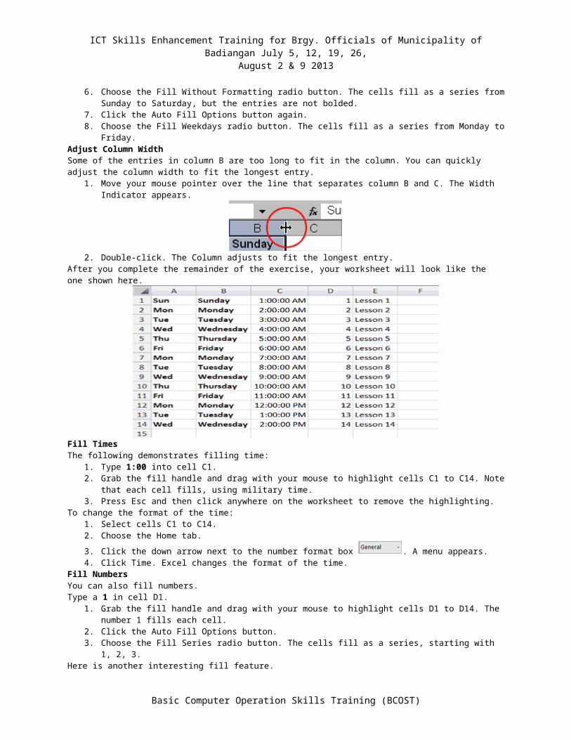
Adjust Column WidthSome of the entries in column B are too long to fit in the column. You can quickly adjust the column width to fit the longest entry.
1. Move your mouse pointer over the line that separates column B and C. The Width Indicator appears.
Basic Computer Operation Skills Training (BCOST)
ICT Skills Enhancement Training for Brgy. Officials of Municipality of Badiangan July 5, 12, 19, 26,
August 2 & 9 2013
2. Double-click. The Column adjusts to fit the longest entry.After you complete the remainder of the exercise, your worksheet will look like the one shown here.
Fill TimesThe following demonstrates filling time:
1. Type 1:00 into cell C1.2. Grab the fill handle and drag with your mouse to highlight cells C1 to C14. Note that each cell fills, using
military time.3. Press Esc and then click anywhere on the worksheet to remove the highlighting.
To change the format of the time:1. Select cells C1 to C14.2. Choose the Home tab.
3. Click the down arrow next to the number format box . A menu appears.4. Click Time. Excel changes the format of the time.
Fill NumbersYou can also fill numbers.Type a 1 in cell D1.
1. Grab the fill handle and drag with your mouse to highlight cells D1 to D14. The number 1 fills each cell.2. Click the Auto Fill Options button.3. Choose the Fill Series radio button. The cells fill as a series, starting with 1, 2, 3.
Here is another interesting fill feature.1. Go to cell E1.2. Type Lesson 1.3. Grab the fill handle and drag with your mouse to highlight cells E1 to E14. The cells fill in as a series: Lesson
1, Lesson 2, Lesson 3, and so on.
Create Headers and FootersYou can use the Header & Footer button on the Insert tab to create headers and footers. A header is text that appears at the top of every page of your printed worksheet. A footer is text that appears at the bottom of every page of your printed worksheet. When you click the Header & Footer button, the Design context tab appears and Excel changes to Page Layout view. A context tab is a tab that only appears when you need it. Page Layout view structures your worksheet so that you can easily change the format of your document. You usually work in Normal view.You can type in your header or footer or you can use predefined headers and footers. To find predefined headers and footers, click the Header or Footer button or use the Header & Footer Elements group's buttons. When you choose a header or footer by clicking the Header or Footer button, Excel centers your choice. The table shown here describes each of the Header & Footer Elements group button options.
Header & Footer Elements
Button Purpose
Basic Computer Operation Skills Training (BCOST)
ICT Skills Enhancement Training for Brgy. Officials of Municipality of Badiangan July 5, 12, 19, 26,
August 2 & 9 2013
Page Number Inserts the page number.
Number of Pages Inserts the number of pages in the document.
Current Time Inserts the current time.
File Path Inserts the path to the document.
File Name Inserts the file name.
Sheet Name Inserts the name of the worksheet.
Picture Enables you to insert a picture.
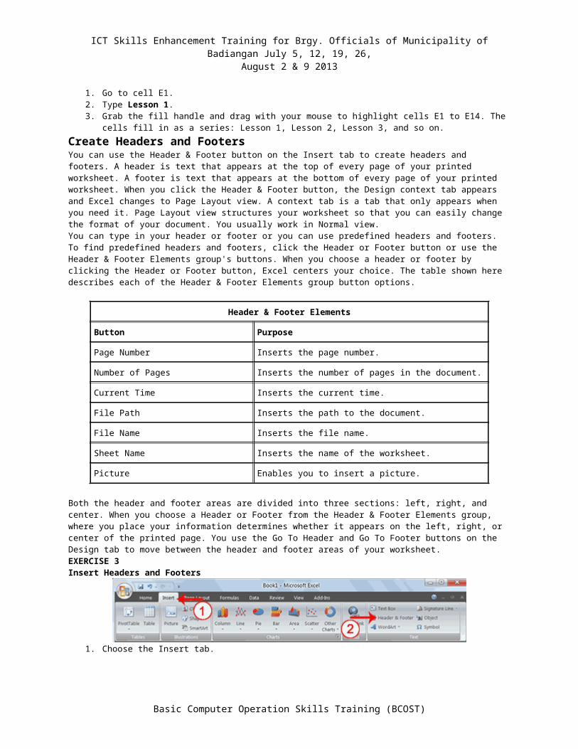
Both the header and footer areas are divided into three sections: left, right, and center. When you choose a Header or Footer from the Header & Footer Elements group, where you place your information determines whether it appears on the left, right, or center of the printed page. You use the Go To Header and Go To Footer buttons on the Design tab to move between the header and footer areas of your worksheet.EXERCISE 3Insert Headers and Footers
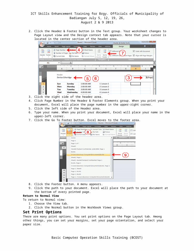
1. Choose the Insert tab.2. Click the Header & Footer button in the Text group. Your worksheet changes to Page Layout view and the
Design context tab appears. Note that your cursor is located in the center section of the header area.
3. Click the right side of the header area.4. Click Page Number in the Header & Footer Elements group. When you print your document, Excel will place
the page number in the upper-right corner.5. Click the left side of the Header area.6. Type your name. When you print your document, Excel will place your name in the upper-left corner.7. Click the Go To Footer button. Excel moves to the footer area.
Basic Computer Operation Skills Training (BCOST)
ICT Skills Enhancement Training for Brgy. Officials of Municipality of Badiangan July 5, 12, 19, 26,
August 2 & 9 2013
8. Click the Footer button. A menu appears.9. Click the path to your document. Excel will place the path to your document at the bottom of every printed
page.Return to Normal ViewTo return to Normal view:
1. Choose the View tab.2. Click the Normal button in the Workbook Views group.
Set Print OptionsThere are many print options. You set print options on the Page Layout tab. Among other things, you can set your margins, set your page orientation, and select your paper size.Margins define the amount of white space that appears on the top, bottom, left, and right edges of your document. The Margin option on the Page Layout tab provides several standard margin sizes from which you can choose.There are two page orientations: portrait and landscape. Paper, such as paper sized 8 1/2 by 11, is longer on one edge than it is on the other. If you print in Portrait, the shortest edge of the paper becomes the top of the page. Portrait is the default option. If you print in Landscape, the longest edge of the paper becomes the top of the page.
Portrait
Landscape
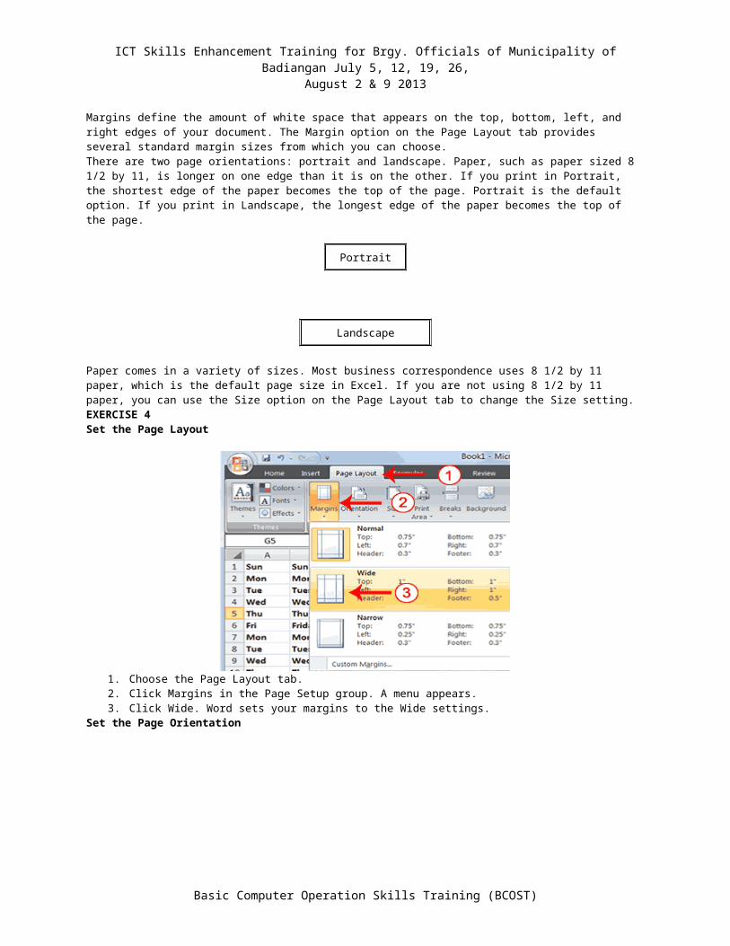
Paper comes in a variety of sizes. Most business correspondence uses 8 1/2 by 11 paper, which is the default page size in Excel. If you are not using 8 1/2 by 11 paper, you can use the Size option on the Page Layout tab to change the Size setting.EXERCISE 4Set the Page Layout
Basic Computer Operation Skills Training (BCOST)

ICT Skills Enhancement Training for Brgy. Officials of Municipality of Badiangan July 5, 12, 19, 26,
August 2 & 9 2013
1. Choose the Page Layout tab.2. Click Margins in the Page Setup group. A menu appears.3. Click Wide. Word sets your margins to the Wide settings.
Set the Page Orientation
1. Choose the Page Layout tab.2. Click Orientation in the Page Setup group. A menu appears.3. Click Landscape. Excel sets your page orientation to landscape.
Set the Paper Size
Basic Computer Operation Skills Training (BCOST)
ICT Skills Enhancement Training for Brgy. Officials of Municipality of Badiangan July 5, 12, 19, 26,
August 2 & 9 2013
1. Choose the Page Layout tab.2. Click Size in the Page Setup group. A menu appears.3. Click the paper size you are using. Excel sets your page size.
PrintThe simplest way to print is to click the Office button, highlight Print on the menu that appears, and then click Quick Print in the Preview and Print the Document pane. Dotted lines appear on your screen, and your document prints. The dotted lines indicate the right, left, top, and bottom edges of your printed pages.You can also use the Print Preview option to print. When using Print Preview, you can see onscreen how your printed document will look when you print it. If you click the Page Setup button while in Print Preview mode, you can set page settings such as centering your data on the page.If your document is several pages long, you can use the Next Page and Previous Page buttons to move forward and backward through your document. If you check the Show Margins check box, you will see margin lines on your document. You can click and drag the margin markers to increase or decrease the size of your margins. To return to Excel, click the Close Print Preview button.You click the Print button when you are ready to print. The Print dialog box appears. You can choose to print the entire worksheet or specific pages. If you want to print specific pages, enter the page numbers in the From and To fields. You can enter the number of copies you want to print in the Number of Copies field.EXERCISE 5Open Print Preview
Basic Computer Operation Skills Training (BCOST)
ICT Skills Enhancement Training for Brgy. Officials of Municipality of Badiangan July 5, 12, 19, 26,
August 2 & 9 2013
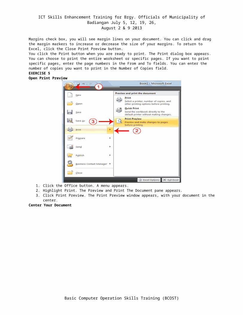
1. Click the Office button. A menu appears.2. Highlight Print. The Preview and Print The Document pane appears.3. Click Print Preview. The Print Preview window appears, with your document in the center.
Center Your Document
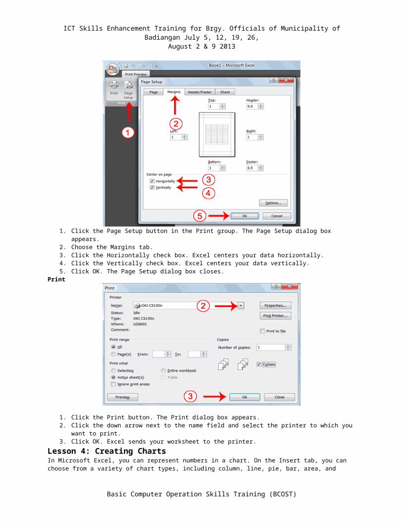
1. Click the Page Setup button in the Print group. The Page Setup dialog box appears.2. Choose the Margins tab.3. Click the Horizontally check box. Excel centers your data horizontally.4. Click the Vertically check box. Excel centers your data vertically.5. Click OK. The Page Setup dialog box closes.
Basic Computer Operation Skills Training (BCOST)
ICT Skills Enhancement Training for Brgy. Officials of Municipality of Badiangan July 5, 12, 19, 26,
August 2 & 9 2013
1. Click the Print button. The Print dialog box appears.2. Click the down arrow next to the name field and select the printer to which you want to print.3. Click OK. Excel sends your worksheet to the printer.
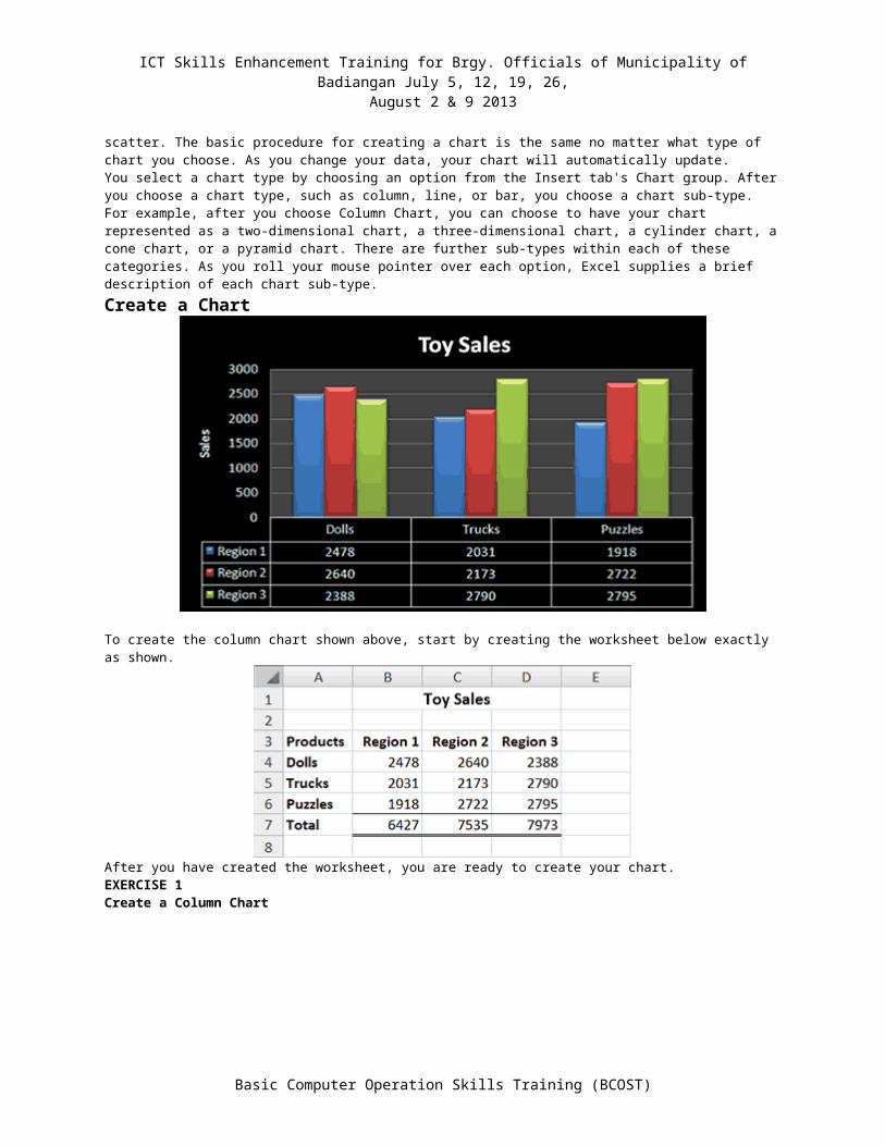
Lesson 4: Creating ChartsIn Microsoft Excel, you can represent numbers in a chart. On the Insert tab, you can choose from a variety of chart types, including column, line, pie, bar, area, and scatter. The basic procedure for creating a chart is the same no matter what type of chart you choose. As you change your data, your chart will automatically update.You select a chart type by choosing an option from the Insert tab's Chart group. After you choose a chart type, such as column, line, or bar, you choose a chart sub-type. For example, after you choose Column Chart, you can choose to have your chart represented as a two-dimensional chart, a three-dimensional chart, a cylinder chart, a cone chart, or a pyramid chart. There are further sub-types within each of these categories. As you roll your mouse pointer over each option, Excel supplies a brief description of each chart sub-type.
Create a Chart
To create the column chart shown above, start by creating the worksheet below exactly as shown.
Basic Computer Operation Skills Training (BCOST)
ICT Skills Enhancement Training for Brgy. Officials of Municipality of Badiangan July 5, 12, 19, 26,
August 2 & 9 2013
After you have created the worksheet, you are ready to create your chart.EXERCISE 1Create a Column Chart
.1. Select cells A3 to D6. You must select all the cells containing the data you want in your chart. You should
also include the data labels.2. Choose the Insert tab.3. Click the Column button in the Charts group. A list of column chart sub-types types appears.4. Click the Clustered Column chart sub-type. Excel creates a Clustered Column chart and the Chart Tools
context tabs appear.
Apply a Chart LayoutContext tabs are tabs that only appear when you need them. Called Chart Tools, there are three chart context tabs: Design, Layout, and Format. The tabs become available when you create a new chart or when you click on a chart. You can use these tabs to customize your chart.You can determine what your chart displays by choosing a layout. For example, the layout you choose determines whether your chart displays a title, where the title displays, whether your chart has a legend, where the legend displays, whether the chart has axis labels and so on. Excel provides several layouts from which you can choose.EXERCISE 2Apply a Chart Layout
Basic Computer Operation Skills Training (BCOST)
ICT Skills Enhancement Training for Brgy. Officials of Municipality of Badiangan July 5, 12, 19, 26,
August 2 & 9 2013
1. Click your chart. The Chart Tools become available.2. Choose the Design tab.3. Click the Quick Layout button in the Chart Layout group. A list of chart layouts appears.4. Click Layout 5. Excel applies the layout to your chart.
Add LabelsWhen you apply a layout, Excel may create areas where you can insert labels. You use labels to give your chart a title or to label your axes. When you applied layout 5, Excel created label areas for a title and for the vertical axis.EXERCISE 3Add labels
Before After
1. Select Chart Title. Click on Chart Title and then place your cursor before the C in Chart and hold down the Shift key while you use the right arrow key to highlight the words Chart Title.
2. Type Toy Sales. Excel adds your title.3. Select Axis Title. Click on Axis Title. Place your cursor before the A in Axis. Hold down the Shift key while
you use the right arrow key to highlight the words Axis Title.4. Type Sales. Excel labels the axis.5. Click anywhere on the chart to end your entry.
Switch DataIf you want to change what displays in your chart, you can switch from row data to column data and vice versa.EXERCISE 4Switch Data
Basic Computer Operation Skills Training (BCOST)

ICT Skills Enhancement Training for Brgy. Officials of Municipality of Badiangan July 5, 12, 19, 26,
August 2 & 9 2013
Before After
1. Click your chart. The Chart Tools become available.2. Choose the Design tab.3. Click the Switch Row/Column button in the Data group. Excel changes the data in your chart.
Change the Style of a ChartA style is a set of formatting options. You can use a style to change the color and format of your chart. Excel 2007 has several predefined styles that you can use. They are numbered from left to right, starting with 1, which is located in the upper-left corner.EXERCISE 5Change the Style of a Chart
1. Click your chart. The Chart Tools become available.2. Choose the Design tab.
3. Click the More button in the Chart Styles group. The chart styles appear.
Basic Computer Operation Skills Training (BCOST)
ICT Skills Enhancement Training for Brgy. Officials of Municipality of Badiangan July 5, 12, 19, 26,
August 2 & 9 2013
4. Click Style 42. Excel applies the style to your chart.
Change the Size and Position of a ChartWhen you click a chart, handles appear on the right and left sides, the top and bottom, and the corners of the chart. You can drag the handles on the top and bottom of the chart to increase or decrease the height of the chart. You can drag the handles on the left and right sides to increase or decrease the width of the chart. You can drag the handles on the corners to increase or decrease the size of the chart proportionally. You can change the position of a chart by clicking on an unused area of the chart and dragging.EXERCISE 6Change the Size and Position of a Chart
1. Use the handles to adjust the size of your chart.2. Click an unused portion of the chart and drag to position the chart beside the data.
Move a Chart to a Chart SheetBy default, when you create a chart, Excel embeds the chart in the active worksheet. However, you can move a chart to another worksheet or to a chart sheet. A chart sheet is a sheet dedicated to a particular chart. By default Excel names each chart sheet sequentially, starting with Chart1. You can change the name.EXERCISE 7Move a Chart to a Chart Sheet
Basic Computer Operation Skills Training (BCOST)
ICT Skills Enhancement Training for Brgy. Officials of Municipality of Badiangan July 5, 12, 19, 26,
August 2 & 9 2013
1. Click your chart. The Chart Tools become available.2. Choose the Design tab.3. Click the Move Chart button in the Location group. The Move Chart dialog box appears.
4. Click the New Sheet radio button.5. Type Toy Sales to name the chart sheet. Excel creates a chart sheet named Toy Sales and places your
chart on it.
Change the Chart TypeAny change you can make to a chart that is embedded in a worksheet, you can also make to a chart sheet. For example, you can change the chart type from a column chart to a bar chart.EXERCISE 8Change the Chart Type
Basic Computer Operation Skills Training (BCOST)
ICT Skills Enhancement Training for Brgy. Officials of Municipality of Badiangan July 5, 12, 19, 26,
August 2 & 9 2013
1. Click your chart. The Chart Tools become available.2. Choose the Design tab.3. Click Change Chart Type in the Type group. The Chart Type dialog box appears.4. Click Bar.5. Click Clustered Horizontal Cylinder.6. Click OK. Excel changes your chart type.
You have reached the end of Lesson 4. You can save and close your file.
Basic Computer Operation Skills Training (BCOST)