Excel 2013

EXCEL® 2013

PART 1

Formula listings:

Formulas usually appear on a separate line in monospace font. For example, I might list the following formula:

=VLOOKUP(StockNumber,PriceList,2,False)

FUNCTIONS, PROCEDURES, AND NAMED RANGES

The names of the Excel worksheet functions appear in all uppercase letters: for example, “Use the SUM function to add the values in column A.”

=SUM(A1:A50)

=sum(a1:a50)

WORKBOOKS AND FILES

Changing the Look of Excel:

choose File. Options to display the Excel Options dialog box. Click the General tab and use the Office Theme drop-down list:

HIDING THE RIBBON

USING OPTIONS ON THE VIEW TAB

Workbook Views group: These options control the overall view. Most of the time, you’ll use

Normal view. Page Layout view is useful if you require precise control over how the pages are laid out. Page Break Preview also shows page breaks, but the display isn’t nearly as nice. The status bar has icons for each of these views. Custom Views enable you to create named views of worksheet settings (for example, a view in which certain columns are hidden).

Show group: The four checkboxes in this group control the visibility of the Ruler (relevant only in Page Layout view), the Formula bar, worksheet gridlines, and row and column headings.

. Zoom group: These commands enable you to zoom the worksheet in or out. Another way to zoom is to use the Zoom slider on the status bar.

CONTROLS ON THE VIEW TAB.

HIDING OTHER ELEMENTS

To hide other elements, you must make a trip to the Advanced tab of the Excel Options dialog box (choose File➜Options).

HIDING THE STATUS BAR

You can also hide the status bar, at the bottom of the Excel window. Doing so, however, requires VBA code.

1. Press Alt+F11 to display the Visual Basic Editor.

2. Press Ctrl+G to display the Immediate window.

3. Type this statement and press Enter:

Application.DisplayStatusBar = False

The status bar will be removed from all open workbook windows. To redisplay the status bar, repeat those instructions, but specify True in the statement

CUSTOMIZING THE QUICK ACCESS TOOLBAR

If you find that you continually need to switch Ribbon tabs because a frequently used command never seems to be on the Ribbon that’s displayed, this tip is for you. The Quick Access toolbar is always visible, regardless of which Ribbon tab is selected. After you customize the Quick Access toolbar, your frequently used commands will always be one click away.

About the Quick Access toolbar

By default, the Quick Access toolbar is located on the left side of the Excel title bar, and it includes three tools:

Save: Saves the active workbook.

Undo: Reverses the effect of the last action.

Redo: Reverses the effect of the last undo

ADDING NEW COMMANDS TO THE QUICK ACCESS TOOLBAR

You can add a new command to the Quick Access toolbar in three ways:

Click the Quick Access toolbar drop-down control, which displays a down-pointing arrow and is located on the right side of the Quick Access toolbar.

Right-click any control on the Ribbon and choose Add to Quick Access Toolbar. The control is added to your Quick Access toolbar, positioned after the last control.

Use the Quick Access Toolbar tab of the Excel Options dialog box. A quick way to access this dialog box is to right-click any Quick Access toolbar or Ribbon control and choose Customize Quick Access Toolbar

THE QUICK ACCESS TOOLBAR DROP-DOWN MENU IS ONE WAY TO ADD A NEW COMMAND TO THE QUICK ACCESS TOOLBAR.

SHOWS THE QUICK ACCESS TOOLBAR TAB OF THE EXCEL OPTIONS DIALOG BOX. THE LEFT SIDE OF THE DIALOG BOX DISPLAYS A LIST OF EXCEL COMMANDS, AND THE RIGHT SIDE SHOWS THE COMMANDS THAT ARE NOW ON THE QUICK ACCESS TOOLBAR. ABOVE THE COMMAND LIST ON THE LEFT IS A DROP-DOWN CONTROL THAT LETS YOU FILTER THE LIST. SELECT AN ITEM FROM THE DROP-DOWN LIST, AND THE LIST DISPLAYS ONLY THE COMMANDS FOR THAT ITEM.

Some of the items in the drop-down list are described here:

Popular Commands: Displays commands that Excel users commonly use.

Commands Not in the Ribbon: Displays a list of commands that you cannot access from the Ribbon.

All Commands: Displays a complete list of Excel commands.

Macros: Displays a list of all available macros.

File Tab: Displays the commands available in the back stage window.

Home Tab: Displays all commands that are available when the Home tab is active.

CUSTOMIZING THE RIBBON

You can customize the Ribbon in these ways:

➤Add a new tab.

➤Add a new group to tab.

➤Add commands to a group.

➤ Remove groups from a tab.

➤ Remove commands from custom groups.

➤Change the order of the tabs.

➤Change the order of the groups within a tab.

➤Change the name of a tab.

➤Change the name of a group.

➤ Reset the Ribbon to remove all customizations

THE CUSTOMIZE RIBBON TAB OF THE EXCEL OPTIONS DIALOG BOX.

UNDERSTANDING PROTECTED VIEW

View. Although it may seem like Excel is trying to keep you from opening your own files, Protected View is all about protecting you from malware.

Malware refers to something that can harm your system. Hackers have figured out several ways to manipulate Excel files so that harmful code can execute. Protected View essentially prevents these types of attacks by opening a file in a protected environment (sometimes called a sandbox).

If you open an Excel workbook that you downloaded from the web, you’ll see a colorful message above the Formula bar (see Figure 4-1). In addition, Excel’s title bar displays the text [Protected View].

THIS MESSAGE TELLS YOU THE WORKBOOK WAS OPENED IN PROTECTED VIEW.

WHAT CAUSES PROTECTED VIEW?

Protected View kicks in for the following:

➤ Files downloaded from the Internet

➤Attachments opened from Outlook

➤ Files that open from potentially unsafe locations, such as your Temporary Internet Files

folder

➤ Files that are blocked by File Block Policy (a feature that allows administrators to define

potentially dangerous files)

➤ Files that were digitally signed, but the signature has expired

You have some control over how Protected View works. To change the settings, choose File➜Options and click Trust Center.

CHANGE THE PROTECTED VIEW SETTINGS IN THE TRUST CENTER DIALOG BOX.

FORCING A WORKBOOK TO OPEN IN NORMAL VIEW

UNDERSTANDING AUTORECOVER

This feature consists of two components:

➤Versions of a workbook are saved automatically, and you can view them.

➤Workbooks that you close without saving are saved as draft versions.

Recovering versions of the current workbook

To see whether any previous versions of the current workbook are available, choose File➜Info. The section labeled Versions lists the available old versions (if any) of the current workbook.

TWO AUTOSAVED VERSIONS OF THIS WORKBOOK ARE AVAILABLE.

USING A WORKBOOK IN A BROWSER

Microsoft’s Office Web Apps enable you to create, view, and edit workbooks directly in a browser. The experience isn’t exactly the same as using the desktop version of Excel, but it’s very similar. A key advantage is that you can access your workbooks from any location, and Excel need not be installed on the computer you use.

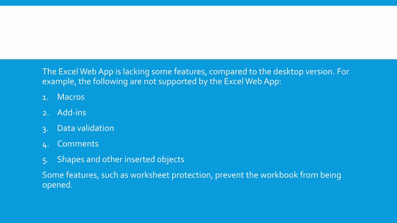
The Excel Web App is lacking some features, compared to the desktop version. For example, the following are not supported by the Excel Web App:

1. Macros

2. Add-ins

3. Data validation

4. Comments

5. Shapes and other inserted objects

Some features, such as worksheet protection, prevent the workbook from being opened.

VIEWING A WORKBOOK IN A WEB BROWSER.

THE DOWNSIDE TO STORING YOUR WORK IN THE CLOUD.

SAVING TO A READ-ONLY FORMAT

If you need to share information in a workbook with someone — and be assured that the information remains intact and isn’t altered — you have several choices.

Send a printed copy

Printing a workbook on paper is the low-tech approach. If the recipient is not nearby, this option may also require some type of delivery service.

Send an electronic copy in the form of a PDF file

PDF files (for Portable Document Format) is a common file format, and just about everyone has software

installed that displays PDF files.

To save a workbook as a PDF file, choose File➜Export➜Create PDF/XPS Document and click the

Create PDF/XPS button to display the Publish as PDF or XPS dialog box. Click the Options button for

additional options:

➤ Choose the pages

➤ Specify what to save (the current range selection, the selected sheet(s), or the entire

workbook

➤ Save document properties and accessibility information

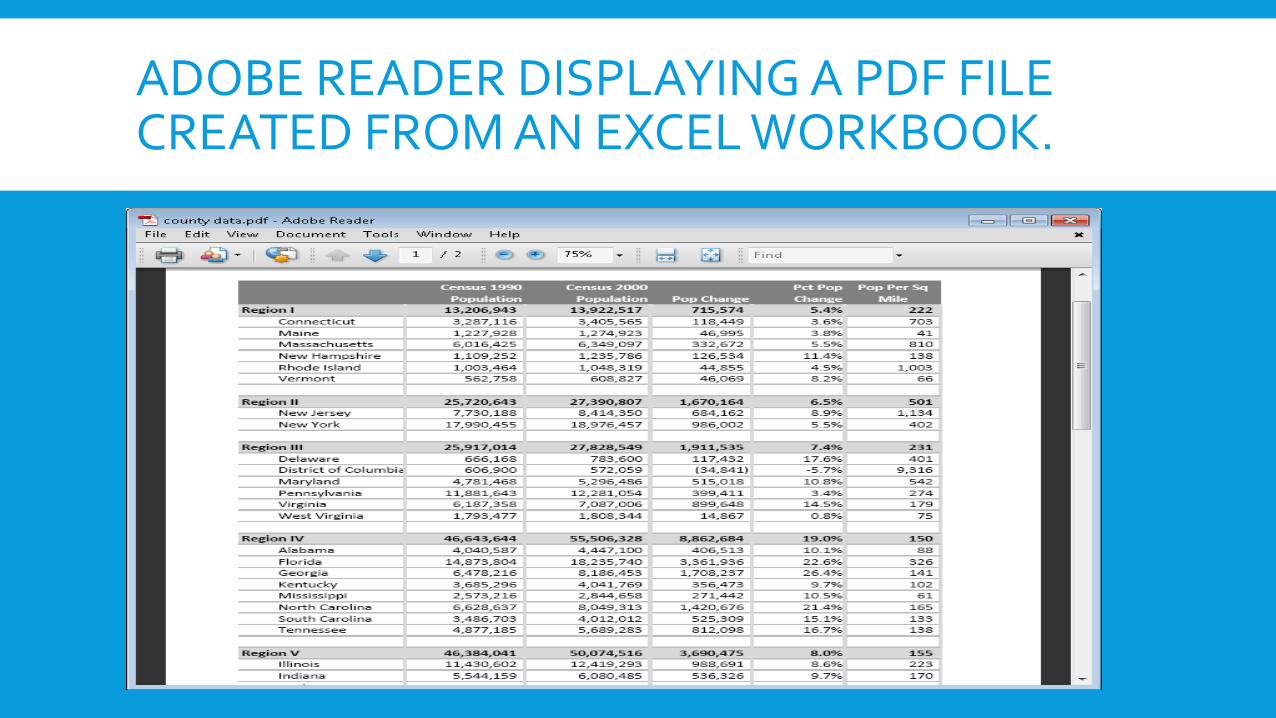
ADOBE READER DISPLAYING A PDF FILE CREATED FROM AN EXCEL WORKBOOK.

SEND AN MHTML FILE

Choose File➜Save As to display the Save As dialog box. Then select Single File Web Page (*.mht, *.mhtl) from the Save As Type drop-down menu.

An Excel workbook saved as an MHTML file and displayed in a web browser.

GENERATING A LIST OF FILENAMES

This tip describes how to retrieve a list of filenames in a folder and display them in a worksheet.

This technique uses an Excel 4 XLM macro function in a named formula. It’s useful because it’s a relativelysimple way of getting a list of filenames into a worksheet — something that normally requires a complex VBA macro.

Start with a new workbook and then follow these steps to create a named formula:

1. Choose Formulas➜Define Name to display the New Name dialog box.

2. Type FileList in the Name field.

3. Enter the following formula in the Refers To field (see Figure 8-1):

=FILES(Sheet1!$A$1)

4. Click OK to close the New Name dialog box.

USING THE NEW NAME DIALOG BOX TO CREATE A NAMED FORMULA.

Note that the FILES function is not a normal worksheet function. Rather, it’s an old XLM style macro function that is intended to be used on a special macro sheet. This function takes one argument (a directory path and a file specification) and returns an array of filenames in that directory that match the file specification.

A normal worksheet formula cannot use these old XLM functions, but named formulas can. After defining the named formula, enter a directory path and file specification into cell A1. For example:

E:\Backup\Excel\*.xl*

Then this formula displays the first file found:

=INDEX(FileList, 1)

If you change the second argument to 2, it displays the second file found, and so on.

The path and file specification is in cell A1. Cell A2 contains this formula,

copied down the column:

=INDEX(FileList,ROW()-1)

The ROW function, as used here, generates a series of consecutive integers: 1, 2, 3, and so on. These

integers are used as the second argument for the INDEX function. Note that cell A21 (and cells below it) displays an error. That’s because the directory has only 19 files, and the formula is attempting to display files that don’t exist. When you change the directory or filespec in cell A1, the formulas update to display the new filenames.

USING AN XLM MACRO IN A NAMED FORMULA CAN GENERATE A LIST OF FILENAMES IN A WORKSHEET

GENERATING A LIST OF SHEET NAMES

Start with a workbook that has lots of worksheets or chart sheets. Then follow these steps to create a

list of the sheet names:

1. Insert a new worksheet to hold the list of sheet names.

2. Choose Formulas➜Define Name to display the New Name dialog box.

3. Type SheetList in the Name field.

4. Enter the following formula in the Refers To field (see Figure 9-1):

=REPLACE(GET.WORKBOOK(1),1,FIND(“]”,GET.WORKBOOK(1)),””)

5. Click OK to close the New Name dialog box.

USING THE NEW NAME DIALOG BOX TO CREATE A NAMED FORMULA.

To generate the sheet names, enter this formula in cell A1, and then copy it down the column:

=INDEX(SheetList,ROW())

shows this formula in the range A1:A10. The workbook has seven sheets, so the formula returns a #REF! error when it attempts to display a nonexistent sheet name. To eliminate this error, modify the formula as follows:

=IFERROR(INDEX(SheetList,ROW()),””)

USING A FORMULA TO DISPLAY A LIST OF SHEET NAMES.

The list of sheet names will adjust if you add sheets, delete sheets, or rename sheets — but the adjustment doesn’t happen automatically. To force the formulas to update, press Ctrl+Alt+F9. If you want the sheet names to adjust automatically when the workbook is calculated, edit the named formula to make it “volatile.”

=REPLACE(GET.WORKBOOK(1),1,FIND(“]”,GET.WORKBOOK(1)),””)&T(NOW())

=HYPERLINK(“#”&A1&”!A1”,”Go to sheet”)

Clicking a hyperlink activates the worksheet and selects cell A1. Unfortunately, Excel doesn’t support hyperlinking to a chart sheet, so you get an error if a hyperlink points to a chart sheet.

THE EXCEL 2013 FILE FORMATS

. xlsx: A workbook file that doesn’t contain macros

.xlsm: A workbook file that contains macros

.xltx: A workbook template file that doesn’t contain macros

.xltm: A workbook template file that contains macros

.xlsa: An add-in file

.xlsb: A binary file that’s similar to the old .xls format but able to accommodate the new features

. xlsk: A backup file

FORMATTING

Working with Merged Cells

To merge cells, just select them and choose Home➜Alignment➜Merge & Center.

For example, shows a worksheet with four sets of merged cells: C2:I2, J2:P2, B4:B8, and B9:B13. The merged cells in column B also use vertical text

This worksheet has four sets of merged cells.

OTHER MERGE ACTIONS

Notice that the Merge and Center button is a drop-down menu. If you click the arrow, you see three additional commands:

➤Merge Across: Lets you select a range and then creates multiple merged cells — one for each row in the selection.

➤Merge Cells: Works just like Merge and Center, except that the content of the upper-left cell is not centered. (It retains its original horizontal alignment.)

➤Unmerge Cells: Unmerges the selected merged cell.

Wrapping text in merged cells is an easy way to display lengthy text. To make text wrap in merged cells, select the merged cells and choose Home.Alignment.WrapText. Use the vertical and horizontal alignment controls in Home.Alignment group to adjust the text position.

LOCATING ALL MERGED CELLS

To find out whether a worksheet contains merged cells, follow these steps:

1. Press Ctrl+F to open the Find and Replace dialog box.

2. Check to be sure the Find What field is empty.

3. Click the Options button to expand the dialog box.

4. Click the Format button to open the Find Format dialog box, where you specify the formatting to find.

5. In the Find Format dialog box, choose the Alignment tab and place a check mark next to

Merged Cells.

6. Click OK to close the Find Format dialog box.

7. In the Find and Replace dialog box, click Find All.

FINDING ALL MERGED CELLS IN A WORKSHEET.

UNMERGING ALL MERGED CELLS

Here’s a quick way to unmerge all merged cells in a worksheet:

1. Select all cells in the worksheet.

A quick way to do so is to click the triangle at the intersection of the row headers and column headers.

2. Click the Home tab.

3. If the Merge & Center command is highlighted, click it.

ALTERNATIVES TO MERGED CELLS

In some cases, you can use Excel’s Center Across Selection command as an alternative to merged cells. This command is useful for centering text across several columns.

1. Enter the text to be centered in a cell.

2. Select the cell that has the text and additional cells to the right of it.

3. Press Ctrl+1 to display the Format Cells dialog box.

4. In the Format Cells dialog box, choose the Alignment tab.

5. In the Text Alignment section, choose the Horizontal drop-down and select Center Across Selection.

6. Click OK to close the Format Cells dialog box.

INDENTING CELL CONTENTS

The legibility of this table can be improved by indenting the text.

THE ALIGNMENT TAB OF THE FORMAT CELLS DIALOG BOX.

SHOWS THE ORIGINAL TABLE AFTER INDENTING THE TEXT. MUCH MORE LEGIBLE!

Indenting the text makes the table easier to read.

USING NAMED STYLES

Throughout the years, one of the most underused features in Excel has been named styles. Named styles make it very easy to apply a set of predefined formatting options to a cell or range. In addition to saving time, using named styles helps to ensure a consistent look across your worksheets. A style can consist of settings for up to six different attributes (which correspond to the tabs in the Format Cells dialog box):

➤Number format

➤Alignment (vertical and horizontal)

➤ Font (type, size, and color)

➤ Borders

➤ Fill (background color)

➤ Protection (locked and hidden)

USING THE STYLE GALLERY

Excel comes with dozens of predefined styles, and you apply these styles in the Style gallery (located in the Home➜Styles group).

Use the Style gallery to work with named styles.

MODIFYING AN EXISTING STYLE

To change an existing style, activate the Style gallery, right-click the style you want to modify, and choose Modify from the shortcut menu. Excel displays the Style dialog box:

Use the Style dialog box to modify named styles.

Cells, by default, use the Normal style. Here’s a quick example of how you can use styles to change

the default font used throughout your workbook:

1. Choose Home➜Styles➜Cell Styles.

Excel displays the list of styles for the active workbook.

2. Right-click Normal in the Styles list and choose Modify.

The Style dialog box opens with the current settings for the Normal style.

3. Click the Format button.

The Format Cells dialog box opens.

4. Click the Font tab and choose the font and size that you want as the default.

5. Click OK to return to the Style dialog box.

6. Click OK again to close the Style dialog box.

The font for all cells that use the Normal style changes to the font that you specified. You can change

any formatting attributes for any style.

Creating new styles

In addition to using the built-in Excel styles, you can create your own styles. This flexibility can be quite handy because it enables you to apply your favorite formatting options very quickly and consistently. To create a new style from an existing formatted cell, follow these steps:

1. Select a cell and apply all the formatting that you want to include in the new style. You can use any of the formatting that’s available in the Format Cells dialog box.

2. After you format the cell to your liking, activate the Style gallery and choose New Cell Style. The Style dialog box opens, along with a proposed generic name for the style. Note that Excel displays the words “By Example” to indicate that it’s basing the style on the current cell.

3. Enter a new style name in the Style Name box. The check boxes show the current formats for the cell. By default, all check boxes are checked.

4. If you don’t want the style to include one or more format categories, remove the check marks from the appropriate boxes.

5. Click OK to create the style and close the dialog box.

CREATING CUSTOM NUMBER FORMATS

Although Excel provides a good variety of built-in number formats, you may find that none of them suits your needs. In such a case, you can probably create a custom number format.

Many Excel users — even advanced users — avoid creating custom number formats because they think that the process is too complicated. In reality, custom number formats tend to look more complex

than they are.

You construct a number format by specifying a series of codes as a number format string. To enter a

custom number format, follow these steps:

1. Press Ctrl+1 to display the Format Cells dialog box.

2. Click the Number tab and select the Custom category.

3. Enter your custom number format in the Type field.

See Tables 16-1 and 16-2 for examples of codes you can use to create your own, custom

number formats.


Parts of a number format string

A custom format string enables you to specify different format codes for four categories of values: positive numbers, negative numbers, zero values, and text. You do so by separating the codes for each category with a semicolon. The codes are arranged in four sections, separated by semicolons:

Positive format; Negative format; Zero format; Text format The following general guidelines determine how many of these four sections you need to specify: . If your custom format string uses only one section, the format string applies to all values.

. If you use two sections, the first section applies to positive values and zeros, and the second section applies to negative values. . If you use three sections, the first section applies to positive values, the second section applies to negative values, and the third section applies to zeros.

. If you use all four sections, the last section applies to text stored in the cell. The following example of a custom number format specifies a different format for each of these types:

[Green]General;[Red]-General;[Black]General;[Blue]General

CODES USED TO CREATE CUSTOM NUMBER FORMATS

Code What It Does

General Displays the number in General format.

# Serves as a digit placeholder that displays only significant digits and doesn’t displayinsignificant zeros.

0 (zero) Serves as a digit placeholder that displays insignificant zeros if a number has fewer digitsthan there are zeros in the format.

? Serves as a digit placeholder that adds spaces for insignificant zeros on either side of thedecimal point so that decimal points align when formatted with a fixed-width font; alsoused for fractions that have varying numbers of digits.

CODES USED IN CREATING CUSTOM FORMATS FOR DATES AND TIMES

Code What It Displays

M The month as a number without leading zeros (1–12)

mm The month as a number with leading zeros (01–12)

mmm The month as an abbreviation (Jan–Dec)

mmmm The month as a full name (January–December)

CREATING A BULLETED LIST

Using a bullet character

You can generate a bullet character by pressing Alt, and typing 0149 on the numeric keypad. If your keyboard lacks a numeric keypad, press the Function key and type numbers using the normal keys.

General”. “

Using an additional column for the bullet characters, or for numbers

SHADING ALTERNATE ROWS USING CONDITIONAL FORMATTING

When you create a table (using Insert➜Tables➜Table), you have the option of formatting the table in such a way that alternate rows are shaded. Alternate row shading can make your spreadsheets easier to read.

Displaying alternate row shading

1. Select the range to format.

2. Choose Home➜Conditional Formatting➜New Rule.

The New Formatting Rule dialog box appears.

3. For the rule type, choose Use a Formula to Determine Which Cells to Format.

4. Enter the following formula in the box labeled Format Values Where This Formulas Is True:

=MOD(ROW(),2)=0


The Format Cells dialog box appears.

6. In the Format Cells dialog box, click the Fill tab and select a background fill color.

7. Click OK to close the Format Cells dialog box, and click OK again to close the New Formatting

Rule dialog box.

USING CONDITIONAL FORMATTING TO APPLY FORMATTING TO ALTERNATE ROWS.

1. Select the range to format.

2. Choose Home.Conditional Formatting.New Rule.

The New Formatting Rule dialog box appears.

3. For the rule type, choose Use a Formula to Determine Which Cells to Format.

4. Enter the following formula in the box labeled Format Values Where This Formulas Is True:

=MOD(ROW(),2)=0



6. In the Format Cells dialog box, click the Fill tab and select a background fill color.

7. Click OK to close the Format Cells dialog box, and click OK again to close the New Formatting

Rule dialog box.

This conditional formatting formula uses the ROW function (which returns the row number) and the MOD function (which returns the remainder of its first argument divided by its second argument). For cells in even-numbered rows, the MOD function returns 0, and cells in that row are formatted.

CREATING CHECKERBOARD SHADING

SHADING GROUPS OF ROWS

Here’s another row shading variation. The following formula shades alternate groups of rows. It produces four rows of shaded rows, followed by four rows of unshaded rows, followed by four more shaded rows, and so on.

=MOD(INT((ROW()-1)/4)+1,2)

For different sized groups, change the 4 to some other value. For example, use this formula to shade alternate groups of two rows:

=MOD(INT((ROW()-1)/2)+1,2)

CONDITIONAL FORMATTING PRODUCES THESE GROUPS OF ALTERNATE SHADED ROWS.

FORMATTING INDIVIDUAL CHARACTERS IN A CELL

To apply formatting to characters within a text string, select those characters first. You can select

them by clicking and dragging your mouse on the Formula bar, or you can double-click the cell and

then click and drag the mouse to select specific characters directly in the cell. A more efficient way to

select individual characters is to press F2 first and then use the arrow keys to move between characters

and use the Shift+arrow keys to select characters.

When the characters are selected, use formatting controls to change the formatting. For example,

you can make the selected text bold, italic, or a different color; you can even apply a different font. If

you right-click, the Mini Toolbar appears, and you can use those controls to change the formatting of

the selected characters.

USING THE FORMAT PAINTER

You’ve probably seen that little Format Painter paint brush icon in the Home➜Clipboardgroup.

Painting basics

Here’s how to use the Format Painter tool in its basic form:

1. Select a cell that contains the formatting that you want to duplicate.

2. Choose Home➜Clipboard➜Format Painter.

The mouse cursor displays a paintbrush to remind you that you’re in Format Painter mode

3. Drag the mouse over another range.

4. Release the mouse button, and the formatting is copied.

Note that the Format Painter is mouse-centric. You cannot use the keyboard to do your painting.

USING THE FORMAT PAINTER TO COPY SHAPE FORMATTING.

INSERTING A WATERMARK

A watermark is an image (or text) that appears on a printed page. A watermark can be a faint company logo or a word, such as DRAFT.

Excel doesn’t have an official command to print a watermark, but you can add a watermark by inserting a picture in the page header or footer. Here’s how to do it:

1. Locate an image on your hard drive that you want to use for the watermark.

2. Choose View.Workbook Views.Page Layout View to enter Page Layout view.

3. Click the center section of the header.

4. Choose Header & Footer Tools.Header & Footer Elements.Picture.

The Insert Picture dialog box appears.

5. Click Browse and locate and select the image you picked in Step 1 (or locate a suitable image

from other sources listed); then click Insert to insert the image.

6. Click outside the header to see your image.

7. To center the image vertically on the page, click the center section of the header and press

Enter a few times before the &[Picture] code.

You¡¯ll need to experiment to determine the number of carriage returns required to push the

image into the body of the document.

8. If you need to adjust the image (for example, to make it lighter), click the center section of

the header and then choose Header & Footer Tools.Header & Footer Elements.Format

Picture; use the Image controls on the Picture tab of the Format Picture dialog box to adjust

the image.

You may need to experiment with the settings to make sure that the worksheet text is legible.

SHOWS AN EXAMPLE OF A HEADER IMAGE (A COPYRIGHT SYMBOL) USED AS A WATERMARK. YOU CANCREATE A SIMILAR EFFECT WITH PLAIN TEXT IN THE HEADER (FOR EXAMPLE, THE WORD DRAFT).

SHOWING TEXT AND A VALUE IN A CELL

If you need to display a number and text in a single cell, Excel gives you three options:

➤Concatenation

➤The TEXT function

➤A custom number format

Assume that cell A1 contains a value, and in a cell somewhere else in your worksheet, you want to display the text Total: along with that value. It looks something like this:

Total: 594.34

You could, of course, put the text Total: in the cell to the left. This section describes the three methods for accomplishing this task using a single cell.

Using concatenation

The following formula concatenates the text Total: with the value in cell A1:

=”Total: “&A1

This solution is the simplest, but it has a problem. The result of the formula is text, rather than a numeric value. Therefore, the cell cannot be used in a numeric formula. Also, the numeric portion will display with no formatting. For example, the formula might return

Total: 1594.34320933

Using the TEXT function

Another solution uses the TEXT function, which displays a value by using a specified number format:

=TEXT(A1,”””Total: “”$#,0.00”)

This formula returns something like this:

Total: $1,594.34

The second argument for the TEXT function is a number format string — the same type of string that

you use when you create a custom number format. Because the number portion is formatted, this

approach looks good. But besides being a bit unwieldy (because of the extra quotation marks), this

formula suffers from the same problem mentioned in the previous section: The result is not numeric.

Using a custom number format

If you want to display text and a value — and still be able to use that value in a numeric formula — the solution is to use a custom number format.

To add text, just create the number format string as usual and put the text within quotation marks.

For this example, the following custom number format does the job:

“Total: “$#,0.00

Even though the cell displays text, Excel still considers the cell contents to be a numeric value. Therefore, you can use this cell in other formulas that perform calculations.

AVOIDING FONT SUBSTITUTION FOR SMALL POINT SIZES

When you specify a font size smaller than eight points, you may notice that the numbers in a column no longer line up correctly. That’s because Excel uses a different (non-proportional) font for small text. Normally, each numeric character takes the same amount of horizontal space — that’s why numbers line up so nicely. But with a proportional font, numeric characters vary in width. The “1”

character is more narrow than the “0” character, for example.

VARIOUS FONT SIZES, WITH FONT SUBSTITUTION ENABLED.

1. Close Excel.

2. Click the Windows Start button and run regedit.exe, the Registry Editor program.

3. In the Registry Editor, navigate to this registry key:

HKEY_CURRENT_USER\Software\Microsoft\Office\15.0\Excel\Options

4. With that registry key selected, choose Edit➜New➜DWORD.

The entry will be named New Value #1.

5. Right-click the entry and choose Rename. Specify FontSub for the entry name.

6. Double-click the FontSub entry.

The Edit DWORD dialog box appears.

7. Specify 0 as the Value Data (the Base, Hexadecimal, or Decimal doesn’t matter), as shown in

Figure 24-2.

8. Click OK to close the Edit DWORD dialog box.

9. Choose File➜Exit to quit Registry Editor.

USING REGISTRY EDITOR TO ADD A NEW VALUE TO THE WINDOWS REGISTRY.

When you restart Excel, you’ll find that Excel no longer uses font substitution for small fonts. When font substitution is disabled, small text will be a bit more difficult to read, but the numbers will continue to line up, and you won’t see the #### display when you zoom out.

Various font sizes, with font substitution disabled.

FORMULAS

Resizing the Formula Bar

In earlier versions of Excel, editing a cell that contains a lengthy formula or lots of text often obscures the worksheet

In older versions of Excel, editing a lengthy formula or a cell that contains lots of text often obscures the worksheet.

CHANGING THE HEIGHT OF THE FORMULA BAR MAKES IT MUCH EASIER TO EDIT LENGTHY FORMULAS AND TEXT, AND YOU CAN STILL VIEW ALL CELLS IN YOUR

WORKSHEET.

MONITORING FORMULA CELLS FROM ANY LOCATION

If you have a large spreadsheet model, you might find it helpful to monitor the values in a few key cells as you change various input cells. The Watch Window feature makes this task very simple. Using the Watch Window, you can keep an eye on any number of cells, regardless of which worksheet or workbook is active. Using this feature can save time and eliminate scrolling and switching among

worksheet tabs and workbook windows.

About the Watch Window

To display the Watch Window, choose Formulas➜Formula Auditing➜WatchWindow. To watch a cell, click the Add Watch button in the Watch Window and then specify the cell in the Add Watch dialog box. When the Add Watch dialog box opens, you can add multiple cells by selecting a range or by pressing Ctrl and clicking individual cells.

For each cell, the Watch Window displays the workbook name, the worksheet name, the cell name (if it has one), the cell address, the current value, and the formula (if it has one).

Excel remembers the cells in a Watch Window, even between sessions. If you close a workbook that contains cells being monitored in the Watch Window, those cells are removed from the Watch Window. But if you reopen that workbook, the cells are displayed again.

About the Watch Window

To display the Watch Window, choose Formulas.Formula Auditing.Watch Window. To watch a cell, click the Add Watch button in the Watch Window and then specify the cell in the Add Watch dialog box. When the Add Watch dialog box opens, you can add multiple cells by selecting a range or by pressing Ctrl and clicking individual cells.

For each cell, the Watch Window displays the workbook name, the worksheet name, the cell name (if it has one), the cell address, the current value, and the formula (if it has one).

Excel remembers the cells in a Watch Window, even between sessions. If you close a workbook that contains cells being monitored in the Watch Window, those cells are rem

Customizing the Watch Window

The Watch Window is a task pane, and you can customize the display by doing any of the following:

➤Click and drag a border to change the size of the task pane.

➤Drag the task pane to an edge of an Excel workbook window, and it becomes docked rather

than free floating.

➤Click and drag the borders in the header to change the width of the columns displayed. By

dragging a column border all the way to the left, you can hide the column.

➤Click one of the headers to sort the contents by that column.

AUTOSUM TRICKS

In the Home➜Editing group and in the Formulas➜Function Library group.

Just activate a cell and click the button, and Excel analyzes the data surrounding the active cell and proposes a SUM formula. If the proposed range is correct, click the AutoSum button again (or press Enter), and the formula is inserted. If you change your mind, press Esc.

Be careful if the range to be summed contains any blank cells. A blank cell will cause Excel to misidentify the complete range. If Excel incorrectly guesses the range to be summed, just select the correct range to be summed and press Enter.

You can also access AutoSum using your keyboard. Pressing Alt+= has exactly the same effect as clicking the AutoSum button.

The AutoSum button can insert other types of formulas. Notice the little arrow on the right side of that button? Click it, and you see four other functions: AVERAGE, COUNT, MAX, and MIN

Using the AutoSum button to insert other functions.

Following are some additional tricks related to AutoSum:

➤ If you need to enter a similar SUM formula into a range of cells, select the entire range before you click the AutoSum button. In this case, Excel inserts the functions for you without asking you — one formula in each of the selected cells. ➤To sum both across and down a table of numbers, select the range of numbers plus an additional column to the right and an additional row at the bottom. Click the AutoSum button, and Excel inserts the formulas that add the rows and the columns. In Figure 28-2, the range

to be summed is D4:G15, so I selected an additional row and column: D4:H16. Clicking the AutoSum buttons puts formulas in row 16 and column H. ➤ If you’re working with a table (created by choosing Insert➜Tables➜Table), using the AutoSum button after selecting the row below the table inserts a Total row for the table and creates formulas that use the SUBTOTAL function rather than the SUM function. The SUBTOTAL function sums only the visible cells in the table, which is useful if you filter the data.

➤Unless you applied a different number format to the cell that will hold the SUM formula, AutoSum applies the same number format as the first cell in the range to be summed.

➤To create a SUM formula that uses only some of the values in a column, select the cells to be summed and then click the AutoSum button. Excel inserts the SUM formula in the first empty cell below the selected range. The selected range must be a contiguous group of cells — a

multiple selection isn’t allowed.

USING AUTOSUM TO INSERT SUM FORMULAS FOR ROWS AND COLUMNS.

ABSOLUTE AND MIXED REFERENCES

When you create a formula that refers to another cell or range, the cell references are usually relative references. When you copy a formula that uses relative references, the cell references adjust to their new location in a relative manner. Assume this formula (which uses relative references) is in cell A13:

=SUM(A1:A12)

If you copy the formula to cell B13, the copied formula is =SUM(B1:B12)

Most of the time, you want cell references to adjust when you copy formulas. That’s why most of the time you use relative references in formulas. But some situations require either absolute or relative references

USING ABSOLUTE REFERENCES

in front of the row part). Here are two examples of formulas that use absolute references:

=$A$1

=SUM($A$1:$F$24)

An absolute cell reference in a formula does not change, even when the formula is copied elsewhere.

For example, assume the following formula is in cell B13:

=SUM($B$1:$B$12)

When you copy this formula to a different cell, the references do not adjust. The copied formula

refers to the same cells as the original, and both formulas return the same result.

When do you use an absolute reference? The answer is simple: The only time you even need to think

about using an absolute reference is if you plan to copy the formula — and you need the copied formula

to refer to the same range as the original.

sheet.

The formula in cell D2 is

=(B2*C2)*$B$7

FORMULA REFERENCES TO THE SALES TAX CELL SHOULD BE ABSOLUTE.

This formula uses relative cell references (B2 * C2) and also an absolute reference to the sales tax cell ($B$7). This formula can be copied to the cells below, and all of the references will be correct. For example, after copying the formula in cell D2, cell D3 contains this formula:

=(B3*C3)*$B$7

The references to the cells in columns B and C are adjusted, but the reference to cell B7 is not — which is exactly what you want.

Using mixed references

In a mixed cell reference, either the column part or the row part of a reference is absolute (and therefore doesn’t change when the formula is copied and pasted). Mixed cell references aren’t used often, but as you see in this tip, in some situations, using mixed references makes your job much easier. Here are two examples of mixed references:

=$A1

=A$1

USING MIXED CELL REFERENCES

The formulas in the table calculate the area for various lengths and widths of a rectangle. Here’s the

formula in cell C3:

=$B3*C$2

Notice that both cell references are mixed. The reference to cell B3 uses an absolute reference for the

column ($B), and the reference to cell C2 uses an absolute reference for the row ($2). As a result, this

formula can be copied down and across, and the calculations are correct. For example, the formula in

cell F7 is

=$B7*F$2

If C3 used either absolute or relative references, copying the formula would produce incorrect

results.

AVOIDING ERROR DISPLAYS IN FORMULAS

Sometimes a formula returns an error, such as #REF! or #DIV/0!. Usually, you want to know when a formula error occurs so you can fix it. But in some cases, you might prefer to simply avoid displaying the error messages.

Column D contains formulas that calculate the average sales volume. For example, cell D2 contains this formula:

=B2/C2

Using the IFERROR function As you can see, the formula displays an error if the cells used in the calculation are empty. If you prefer to hide those error values, you can do so by using an IFERROR function. This function takes two arguments: The first argument is the expression that’s checked for an error, and the second is the

value to return if the formula evaluates to an error. The formula presented earlier can be rewritten as

=IFERROR(B2/C2,””)

USING AN IFERROR FUNCTION TO HIDE ERROR VALUES.

USING THE ISERROR FUNCTION

in cell D1:

=IF(ISERROR(B2/C2),””,B2/C2)

The ISERROR function returns TRUE if its argument evaluates to an error. In such a case, the IF function returns an empty string. Otherwise, the IF function returns the calculated value.

This method of avoiding an error display is a bit more complicated, and it’s also less efficient because the formula is actually evaluated two times if it doesn’t return an error. Therefore, unless you require compatibility with Excel 2003 or earlier versions, you should use the IFERROR functions.

CREATING WORKSHEET-LEVEL NAMES

THE NAME MANAGER MAKES IT EASY TO DISTINGUISH BETWEEN WORKBOOK-LEVEL NAMES AND WORKSHEETLEVEL NAMES.

USING NAMED CONSTANTS

This tip describes a useful technique that can remove some clutter from your worksheets: named constants.

Consider a worksheet that generates an invoice and calculates sales tax for a sales amount. The common approach is to insert the sales tax rate value into a cell and then use this cell reference in your formulas. To make things easier, you probably would name this cell something like SalesTax.

You can store your sales tax rate by using a name (and avoid using a cell).

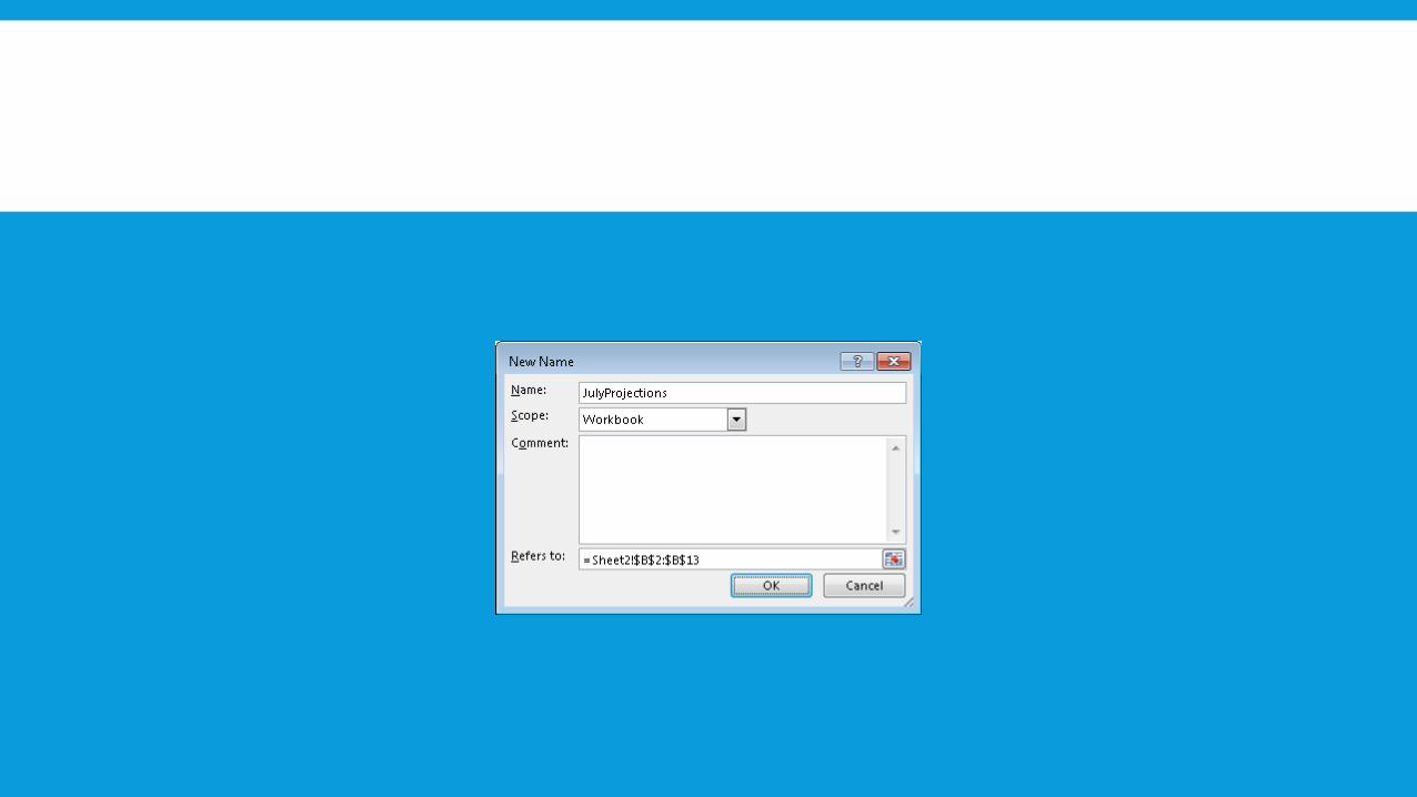
1. Choose Formulas➜Defined Names➜Define Name to open the New Name dialog box.

2. Type the name (in this case, SalesTax) into the Name field.

3. Specify Workbook as the scope for the name. If you want the name to be valid only on a particular worksheet, specify the worksheet in the Scope field of the New Name dialog box.

4. Click the Refers To field, delete its contents, and replace it with a simple formula, such as =7.5%.

5. Click OK to close the dialog box.

DEFINING A NAME THAT REFERS TO A CONSTANT

The preceding steps create a named formula that doesn’t use any cell references. To try it out, enter the following formula into any cell:

=SalesTax

This simple formula returns .075, the result of the formula named SalesTax. Because this named formula always returns the same result, you can think of it as a named constant. And you can use this constant in a more complex formula, such as this one:

=A1*SalesTax

A named constant can also consist of text. For example, you can define a constant for a company’s name. You can use the New Name dialog box to create the following formula, named MSFT:

=”Microsoft Corporation”

Then you can use a cell formula, such as this one:

=”Annual Report: “&MSFT

This formula returns the text Annual Report: Microsoft Corporation.

SENDING PERSONALIZED E-MAIL FROM EXCEL

About the HYPERLINK function

The HYPERLINK function creates a link that, when clicked, activates your default browser and navigates to a web page. The function takes two arguments: the URL and the text that’s displayed in the cell. For example, this formula creates a link to my website:

=HYPERLINK(“http://spreadsheetpage.com”,”Spreadsheet Page”)

A URL can also contain an e-mail address. When clicked, the hyperlink opens the new message window of your default e-mail client, with the e-mail address in the “To” field. Here’s an example:

=HYPERLINK(“mailto:[email protected]”,”Email support”)

You can also include a subject line. Here’s an example of the first argument for the HYPERLINK function

that includes an e-mail subject line:

“mailto:[email protected]?subject=Help!”

In addition, you can include a short default message:

“mailto:[email protected]?subject=Help me!&body=I don’t understand this.”

Things get a bit more complicated if you want to include a line break in the message body. If that’s the case, you need to “percent encode” the line break by using this code: %0A. Here’s an example that inserts two line breaks into the e-mail body:

“mailto:[email protected]?subject=Help me!&body=I don’t understand

this.%0A%0AYour customer”

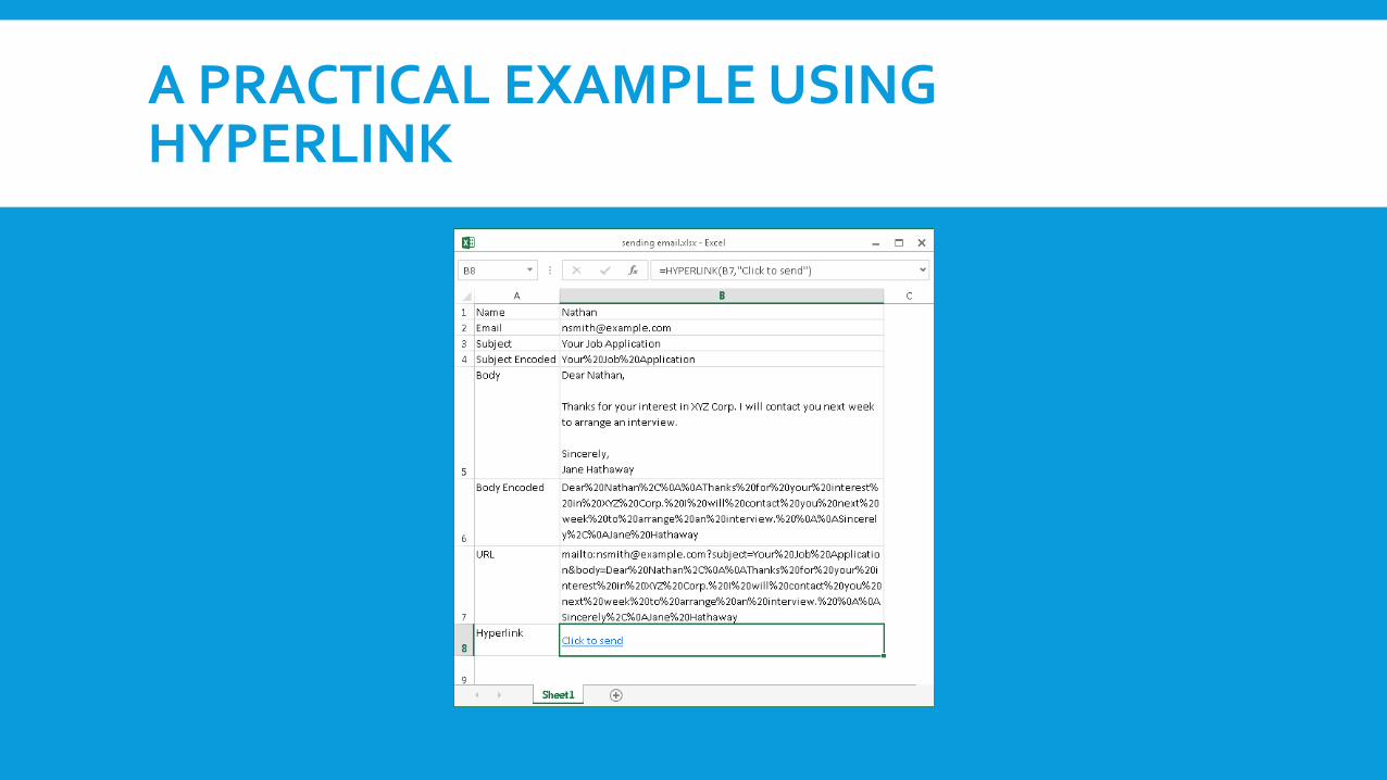
A PRACTICAL EXAMPLE USING HYPERLINK

Here’s a description of each cell:

➤ B1: The first name of the e-mail recipient.

➤ B2: The e-mail address.

➤ B3: The subject line for the e-mail address.

➤ B4: The subject line, encoded using this formula:

=ENCODEURL(B3)

➤ B5: The body of the message. This cell uses wrap text formatting, and line breaks were

entered by using Alt+Enter.

➤ B6: The body text, encoded using this formula:

=ENCODEURL(B5)

➤ B7: The first argument for the HYPERLINK function, constructed by concatenating text and

cells. The formula is

=”mailto:”&B2&”?subject=”&(B4)&”&body=”&B6&””

➤ B8: This cell contains a formula that uses the HYPERLINK function:

=HYPERLINK(B7,”Click to send”)

LOOKING UP AN EXACT VALUE

The VLOOKUP and HLOOKUP functions are useful if you need to return a value from a table (in a range) by looking up another value.

The classic example of a lookup formula involves an income tax rate schedule

The tax rate schedule shows the income tax rates for various income levels. The following formula (in cell B3) returns the tax rate for the income value in cell B2:

=VLOOKUP(B2,D2:F7,3)

The tax table example demonstrates that VLOOKUP and HLOOKUP don’t require an exact match between the value to be looked up and the values in the lookup table. In some cases, though, you might require a perfect match. For example, when looking up an employee number, close doesn’t count. You require an exact match for the number. To look up only an exact value, use the VLOOKUP (or HLOOKUP) function with the optional fourth argument set to FALSE.

shows a worksheet with a lookup table that contains employee numbers (column D) and employee names (column E). The formula in cell B2, which follows, looks up the employee number entered in cell B1 and returns the corresponding employee name:

=VLOOKUP(B1,D1:E11,2,FALSE)

If you prefer to see something other than #N/A when the employee number isn’t found, you can use the IFERROR function to test for the #N/A result (using the ISNA function) and substitute a different string. The following formula displays the text “Not Found” rather than #N/A:

=IFERROR(VLOOKUP(B2,D1:E11,2,FALSE),”Not Found”)

The IFERROR function was introduced in Excel 2007, so if your workbook must be compatible with Excel 2003 and earlier versions, use this formula:

=IF(ISERROR(VLOOKUP(B2,D1:E11,2,FALSE)),”Not Found”,

VLOOKUP(B2,D1:E11,2,FALSE)

PERFORMING A TWO-WAY LOOKUP

A two-way lookup identifies the value at the intersection of a column and a row. This tip describes two methods to perform a two-way lookup.

Using a formula

A worksheet with a range that displays product sales by month. To retrieve sales

for a particular month and product, the user enters a month in cell B1 and a

product name in cell B2.

TO SIMPLIFY THE PROCESS, THE WORKSHEET USES THE NAMED RANGES SHOWN IN THE FOLLOWING MINITABLE.

The following formula (in cell B4) uses the MATCH function to return the position of the Month

within the MonthList range. For example, if the month is January, the formula returns 2 because January is the second item in the MonthList range (the first item is a blank cell, D1):

=MATCH(Month,MonthList,0)

The formula in cell B5 works similarly but uses the ProductList range:

=MATCH(Product,ProductList,0)

The final formula, in cell B6, returns the corresponding sales amount. It uses the INDEX function with

the results from cells B4 and B5:

=INDEX(Table,B4,B5)

You can combine these formulas into a single formula, as shown here:

=INDEX(Table,MATCH(Month,MonthList,0),MATCH(Product,ProductList,0))

Using implicit intersection

The second method to accomplish a two-way lookup is quite a bit simpler, but it requires that you create a name for each row and column in the table.

A quick way to name each row and column is to select the table and choose Formulas➜Defined Names➜Create from Selection. In the Create Names from Selection dialog box, specify that the names are in the top row and left column (see Figure 35-2). Click OK, and Excel creates the names.

After creating the names, you can use a simple formula to perform the two-way lookup, such as

=Sprockets July

This formula, which uses the range intersection operator (a space), returns July sales data for Sprockets.

PERFORMING A TWO-COLUMN LOOKUP

Some situations may require a lookup based on the values in two columns.

The following array formula displays the corresponding code for an automobile make and model:

=INDEX(Code,MATCH(Make&Model,Range1&Range2,0))

After you create this new table, you can use a simpler formula to perform the lookup:

=VLOOKUP(Make&Model,H2:I12,2)

CALCULATING HOLIDAYS

Determining the date for a particular holiday can be tricky. Some holidays, such as New Year’s Day and Independence Day (U.S.), are no-brainers because they always occur on the same date. For these kinds of holidays, you can simply use the DATE function. For example, to calculate New Year’s Day (which always falls on January 1) for a specific year stored in cell A1, you can enter this function:

=DATE(A1,1,1)

Other holidays are defined in terms of a particular occurrence of a particular weekday in a particular month. For example, Labor Day in the U.S. falls on the first Monday in September.The formulas that follow all assume that cell A1 contains a year value (for example, 2013). Notice that because New Year’s Day, Independence Day, Veterans Day, and Christmas Day all fall on the same days of the year, their dates can be calculated by using the simple DATE function.

New Year’s Day

This holiday always falls on January 1:

=DATE(A1,1,1)

Martin Luther King Jr. Day

This holiday occurs on the third Monday in January. The following formula calculates Martin Luther

King Jr. Day for the year in cell A1

=DATE(A1,1,1)+IF(2<WEEKDAY(DATE(A1,1,1)),7-WEEKDAY(DATE(A1,1,1))

+2,2-WEEKDAY(DATE(A1,1,1)))+((3-1)*7)

Presidents’ Day

Presidents’ Day occurs on the third Monday in February. This formula calculates Presidents’ Day for

the year in cell A1:


+2,2-WEEKDAY(DATE(A1,2,1)))+((3-1)*7)

Easter

Calculating the date for Easter is difficult because of the complicated manner in which Easter is determined.

Easter Day is the first Sunday after the next full moon occurs after the vernal equinox. I found

these formulas to calculate Easter on the web. I have no idea how they work. They don’t work if your

workbook uses the 1904 date system.

=DOLLAR((“4/”&A1)/7+MOD(19*MOD(A1,19)-7,30)*14%,)*7-6

This one is slightly shorter, but equally obtuse:

=FLOOR(“5/”&DAY(MINUTE(A1/38)/2+56)&”/”&A1,7)-34

Memorial Day

The last Monday in May is Memorial Day. This formula calculates Memorial Day for the year in cell A1:


+2,2-WEEKDAY(DATE(A1,6,1)))+((1-1)*7)-7

Notice that this formula calculates the first Monday in June and then subtracts 7 from the result, to

return the last Monday in May.

Independence Day

The Independence Day holiday always falls on July 4:

=DATE(A1,7,4)

Labor Day

Labor Day occurs on the first Monday in September. This formula calculates Labor Day for the year in cell A1:

=DATE(A1,9,1)+IF(2<WEEKDAY(DATE(A1,9,1)),7-WEEKDAY(DATE(A1,9,1)) +2,2-WEEKDAY(DATE(A1,9,1)))+((1-1)*7)

Columbus Day

The Columbus Day holiday occurs on the second Monday in October. The following formula calculates Columbus Day for the year in cell A1:

=DATE(A1,10,1)+IF(2<WEEKDAY(DATE(A1,10,1)),7-WEEKDAY(DATE(A1,10,1)) +2,2-WEEKDAY(DATE(A1,10,1)))+((2-1)*7)

Veterans Day

The Veterans Day holiday always falls on November 11:

=DATE(A1,11,11)

Thanksgiving Day

Thanksgiving Day is celebrated on the fourth Thursday in November. This formula calculates Thanksgiving Day for the year in cell A1:


+5,5-WEEKDAY(DATE(A1,11,1)))+((4-1)*7)

Christmas Day

Christmas Day always falls on December 25:

=DATE(A1,12,25)

Calculating a Person’s Age

Calculating a person’s age is a bit tricky because the calculation depends on not only the current year but also the current day. And then you have to consider the complications resulting from leap years. In this tip, I present three methods to calculate a person’s age. These formulas assume that cell B1

contains the date of birth (for example, 2/16/1952) and that cell B2 contains the current date (calculated with the TODAY function).

Method 1

The following formula subtracts the date of birth from the current date and divides by 365.25. The INT function then eliminates the decimal part of the result: =INT((B2-B1)/365.25) This formula isn’t 100 percent accurate because it divides by the average number of days in a year.

For example, consider a child who is exactly one year old. This formula returns 0, not 1. Method 2 A more accurate way to calculate age uses the YEARFRAC function:

=INT(YEARFRAC(B2, B1))

The YEARFRAC function is normally used in financial calculations, but it works just fine for calculating ages. This function calculates the fraction of the year represented by the number of whole days

between two dates. Using the INT function eliminates the fraction and returns an integer that represents full years.

Method 3

The third method for calculating age uses the DATEDIF function. This undocumented function isn’t described in the Excel Help system:

=DATEDIF(B1,B2,”Y”)

RETURNING THE LAST NONBLANK CELL IN ACOLUMN OR ROW

Suppose that you update a worksheet frequently by adding new data to its columns. You might need a way to reference the last value in a particular column (the value most recently entered). This tip presents three ways to accomplish this.

Use a formula to return the last non-empty cell in columns B:D.

sCell counting method

The formulas in G4, G5, and G6 are

=INDEX(B:B,COUNTA(B:B))

=INDEX(C:C,COUNTA(C:C))

=INDEX(D:D,COUNTA(D:D))

These formulas use the COUNTA function to count the number of non-empty cells in column C. This value is used as the second argument for the INDEX function. For example, in column B the last value is in row 6, COUNTA returns 6, and the INDEX function returns the 6th value in the column. The preceding formulas work in most, but not all, situations. If the column has one or more empty cells interspersed, determining the last nonblank cell is a bit more challenging because the COUNTA function doesn’t count the empty cells.

Array formula method

The following array formula returns the contents of the last non-empty cell in the first 500 rows of

column B, even if column B contains blank cells:

=INDEX(B:B,MAX(ROW(B:B)*(B:B<>””)))

Press Ctrl+Shift+Enter (not just Enter) to enter an array formula

You can, of course, modify the formula to work with a column other than column B. To use a different column, change the four column references from B to whatever column you need. You can’t use this formula, as written, in the same column in which it’s working. Attempting to do so generates a circular reference. You can, however, modify it. For example, to use the function in cell B1, change the references so that they begin with row 2 rather than the entire columns. For example, use B2:B1000 to return the last non-empty cell in the range B2:B1000. The following array formula is similar to the previous formula, but it returns the last non-empty cell in a row (in this case, row 1):

=INDEX(1:1,MAX(COLUMN(1:1)*(1:1<>””))) To use this formula for a different row, change the three 1:1 row references to correspond to the correct row number.

Standard formula method

The final method uses a standard (non-array) formula, and is rather cryptic. This formula returns the

last non-empty cell in column B:

=LOOKUP(2,1/(B:B<>””),B:B)

This formula ignores error values, so if the last non-empty cell contains an error (such as #DIV/0!), the formula returns the last non-empty, non-error cell.

The following formula returns the last non-empty, non-error cell in row 1:

=LOOKUP(2,1/(1:1<>””),1:1)

Rounding currency values

Often, you need to round currency values. For example, a calculated price might be a number like $45.78923. In such a case, you want to round the calculated price to the nearest penny. This process might sound simple, but you can round this type of value in one of three ways:

. Round it up to the nearest penny. . Round it down to the nearest penny. . Round it to the nearest penny (the rounding can be up or down). The following formula assumes that a dollar-and-cents value is in cell A1. The formula rounds the value to the nearest penny. For example, if cell A1 contains $12.421, the formula returns $12.42. =ROUND(A1,2)

If you need to round up the value to the nearest penny, use the CEILING.MATH function. The following formula rounds up the value in cell A1 to the nearest penny (if, for example, cell A1 contains $12.421, the formula returns $12.43):

=CEILING.MATH(A1,0.01)

To round down a dollar value, use the FLOOR.MATH function. The following formula, for example, rounds down the dollar value in cell A1 to the nearest penny (if cell A1 contains $12.421, the formula returns $12.42):

=FLOOR.MATH(A1,0.01)

To round up a dollar value to the nearest nickel, use this formula:

=CEILING.MATH(A1,0.05)

Using the INT and TRUNC functions

On the surface, the INT and TRUNC functions seem similar. Both convert a value to an integer. The TRUNC function simply removes the fractional part of a number. The INT function rounds down a number to the nearest integer, based on the value of the fractional part of the number.

In practice, INT and TRUNC return different results only when using negative numbers. For example,

the following formula returns –14.0:

=TRUNC(-14.2)

The next formula returns –15.0 because –14.2 is rounded down to the next lower integer:

=INT(-14.2)

The TRUNC function takes an additional (optional) argument that’s useful for truncating decimal values.

For example, the following formula returns 54.33 (the value truncated to two decimal places):

=TRUNC(54.3333333,2)

Rounding to n significant digits

In some situations, you may need to round a value to a particular number of significant digits. For example, you may want to express the value 1,432,187 in terms of two significant digits (that is, as 1,400,000). The value 84,356 expressed in terms of three significant digits is 84,300.

If the value is a positive number with no decimal places, the following formula does the job. This formula rounds the number in cell A1 to two significant digits. To round to a different number of significant digits, replace the 2 in this formula with a different number:

=ROUNDDOWN(A1,2-LEN(A1))

For non-integers and negative numbers, the solution is a bit trickier. The following formula provides a more general solution that rounds the value in cell A1 to the number of significant digits specified in cell A2. This formula works for positive and negative integers and non-integers:

=ROUND(A1,A2-1-INT(LOG10(ABS(A1))))

For example, if cell A1 contains 1.27845 and cell A2 contains 3, the formula returns 1.28000 (the value, rounded to three significant digits).

Converting Between Measurement

Systems

You know the distance from New York to London in miles, but your European office needs the numbers in kilometers. What’s the conversion factor?

The Excel CONVERT function can convert between a variety of measurements in these categories:

. Area

. Distance

. Energy

. Force

. Information

. Magnetism

. Power

. Pressure

. Speed

(or liquid measure)

abbreviations are commonly used, but others aren’t. And, of course, you must use the exact abbreviation.

The CONVERT function is even more versatile than it seems. When using metric units, you can apply a multiplier. In fact, the first example I presented uses a multiplier. The unit abbreviation for the third argument is m, for meters. I added the kilo-multiplier (k) to express the result in kilometers.

In some situations, the CONVERT function requires some creativity. For example, if you need to convert 100 km/hour into miles/sec, the formula requires two uses of the CONVERT function:

=CONVERT(100,”km”,”mi”)/CONVERT(1,”hr”,”sec”)

The CONVERT function has been significantly enhanced in Excel 2013 and supports dozens of new measurement units.

COUNTING NONDUPLICATED ENTRIES IN ARANGE

Column A has a list of animals, and the goal is to count the number of different

animals in the list. The formula in cell B2 returns 6, which is the number of nonduplicated animals.

This formula (an array formula, by the way) is

=SUM(1/COUNTIF(A1:A10,A1:A10))

USE AN ARRAY FORMULA TO COUNT THE NUMBER OF NONDUPLICATED ENTRIES IN A RANGE.

The preceding array formula works fine unless the range contains one or more empty cells. The following modified version of this array formula uses the IFERROR function to overcome this problem:

=SUM(IFERROR(1/COUNTIF(A1:A10,A1:A10),0))

The preceding formulas work with both values and text. If the range contains only numeric values or blank cells (but no text), you can use the following formula (which isn’t an array formula) to count the number of nonduplicated values:

=SUM(N(FREQUENCY(A1:A10,A1:A10)>0))

USING THE AGGREGATE FUNCTION

One of the most versatile functions available in Excel is AGGREGATE, which was introduced in Excel

2010. You can use this multipurpose function to sum values, calculate an average, count entries, and

more. What makes this function useful is that it can (optionally) ignore values in hidden rows and

error values. In some cases, you can use AGGREGATE to replace a complex array formula.

The AGGREGATE function takes three arguments, but for some functions, an additional argument is

required.

The first argument for the AGGREGATE function is a value between 1 and 19 that determines the

type of calculation to perform. The calculation type, in essence, is one of Excel’s other functions.

Table 45-1 contains a list of these values, with the function it mimics.

1 AVERAGE

2 COUNT

3 COUNTA

4 MAX

5 MIN

6 PRODUCT

7 STDEV.S

8 STDEV.P

9 SUM

10 VAR.S

11 VAR.P

12 MEDIAN

13 MODE.SNGL

14* LARGE

=AVERAGE(D2:D9)

The formula in cell D12 uses the AGGREGATE function, with the option to ignore error values:

=AGGREGATE(1,6,D2:D9)

MAKING AN EXACT COPY OF A RANGE OFFORMULAS

that cell D1 contains this formula:

=A1*B1

When you copy this cell, the two cell references are changed relative to the destination. If you copy

D1 to D12, for example, the copied formula is

=A12*B12

1. Put Excel in Formula view mode.

To toggle Formula view mode, choose Formulas.Formula Auditing.Show Formulas.

2. Select the range to copy. In this case, A1:D10 on Sheet1.

3. Press Ctrl+C to copy the range.

4. Launch the Windows Notepad text editor.

5. Press Ctrl+V to paste the copied data into Notepad.

6. In Notepad, press Ctrl+A to select all of the text, followed by Ctrl+C to copy the text.

7. Activate Excel and activate the upper-left cell where you want to paste the formulas (in this

example, A13 on Sheet2) and make sure that the sheet you¡¯re copying to is in Formula view

mode.

8. Press Ctrl+V to paste.

9. Choose Formulas.Formula Auditing.Show Formulas to toggle out of Formula view mode.

USING THE BACKGROUND ERROR-CHECKINGFEATURES

To display this dialog box, choose File➜Options.

You turn error checking on or off by using the Enable Background Error Checking check box. In addition, you can specify which types of errors to check by selecting check boxes in the Error Checking Rules section.

the cell from subsequent error checks. You can select a range of formulas, and then choose Ignore Error to ignore them all. All previously ignored errors can be reset so that they appear again. (Click the Reset Ignored Errors button in the Excel Options dialog box.)

Even if you don’t use the automatic error-checking option, you can choose the Formulas➜Formula Auditing➜Error Checking command to open a dialog box that displays each potential error cell in sequence, much like using a spell-checking feature. the Error Checking dialog box. Note that because it’s a modeless dialog box, you can still access your worksheet when the Error

Checking dialog box is open.

USING THE ERROR CHECKING DIALOG BOX TO CYCLE THROUGH POTENTIAL ERRORS IDENTIFIED BY EXCEL.

USING THE INQUIRE ADD-IN

Office 2013 Professional Plus includes a handy auditing add-in called Inquire. To install this add-in,follow these steps:

1. Choose File➜Options to display the Excel Options dialog box.

2. Click the Add-Ins tab.

3. Choose COM Add-Ins from the Manage drop-down list and click Go to display the COM Add-Ins dialog box.

4. In the COM Add-Ins dialog box, select the Inquire item and click OK.

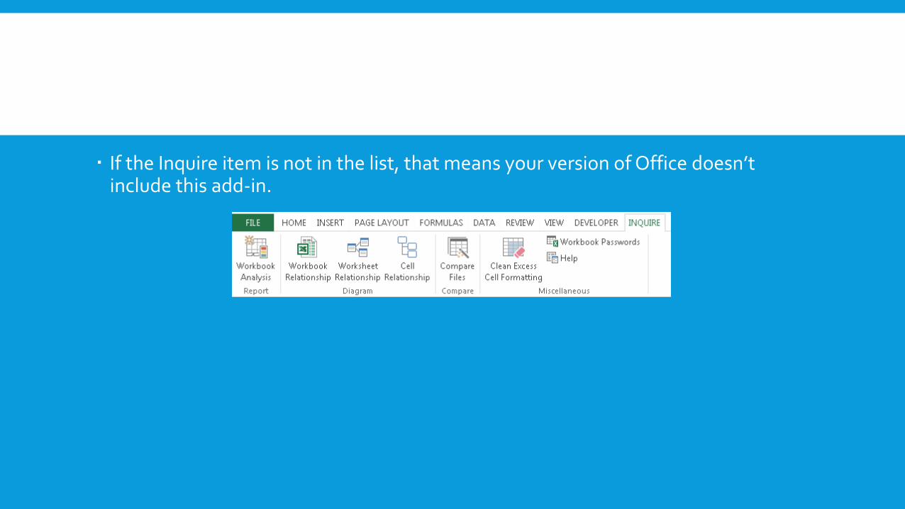
If the Inquire item is not in the list, that means your version of Office doesn’t include this add-in.

Workbook analysis

To analyze the active workbook, choose Inquire➜Report➜Workbook Analysis to display the Workbook Analysis Report dialog box shown in Figure 48-2. Use the Items list on the left to select an analysis item, and the results (if any) appear in the Results section on the right. To create a report (in a new workbook), select the items to include in the report and choose Excel Export. The report is very detailed and is a good way to document an Excel workbook.

HIDING AND LOCKING YOUR FORMULAS

Hiding and locking formula cells

Follow these steps to hide all of the formula cells on the active worksheet:

1. Select a single cell, and choose Home➜Editing➜Find & Select➜Go To Special. Excel displays

the Go To Special dialog box.

2. In the Go To Special dialog box, choose the Formulas option and make sure all four check

boxes are checked (see Figure 49-1).

3. Click OK, and Excel selects all of the formula cells.

4. Right-click any of the selected formula cells and choose Format Cells from the shortcut menu.


5. Click the Protection tab to display the Locked and Hidden checkboxes.

6. Check both the Locked and the Hidden check boxes.


UNLOCKING NONFORMULA CELLS

Follow these steps to unlock all of the nonformula cells:

1. Select a single cell, and choose Home➜Editing➜Find & Select➜Go To Special. Excel displays

the Go To Special dialog box.

2. In the Go To Special dialog box, choose the Constants option and make sure all four check

boxes are checked.

3. Click OK, and Excel selects all of the constant (nonformula) cells.

4. Right-click any of the selected formula cells and choose Format Cells from the shortcut

menu.


5. Click the Protection tab to display the Locked and Hidden check boxes.

6. Uncheck both the Locked and the Hidden check boxes.


Protecting the worksheet

The steps in the two previous sections have no effect unless the worksheet is protected. Follow these

steps to protect the worksheet:

1. Choose Review➜Changes➜Protect Sheet to access the Protect Sheet dialog box

2. In the Protect Sheet dialog box, specify a password (if desired). If you don’t specify a password,anyone can unprotect the sheet and see (or modify) the formulas.

3. Click OK, and you will be prompted to reenter the password.

USING THE INDIRECT FUNCTION

To make a formula more flexible, you can use the Excel INDIRECT function to create a range reference.This rarely used function accepts a text argument that resembles a range reference and then converts the argument to an actual range reference. When you understand how this function works, you can use it to create more powerful interactive spreadsheets.

Specifying rows indirectly

=SUM(INDIRECT(“B”&E2&”:B”&E3))

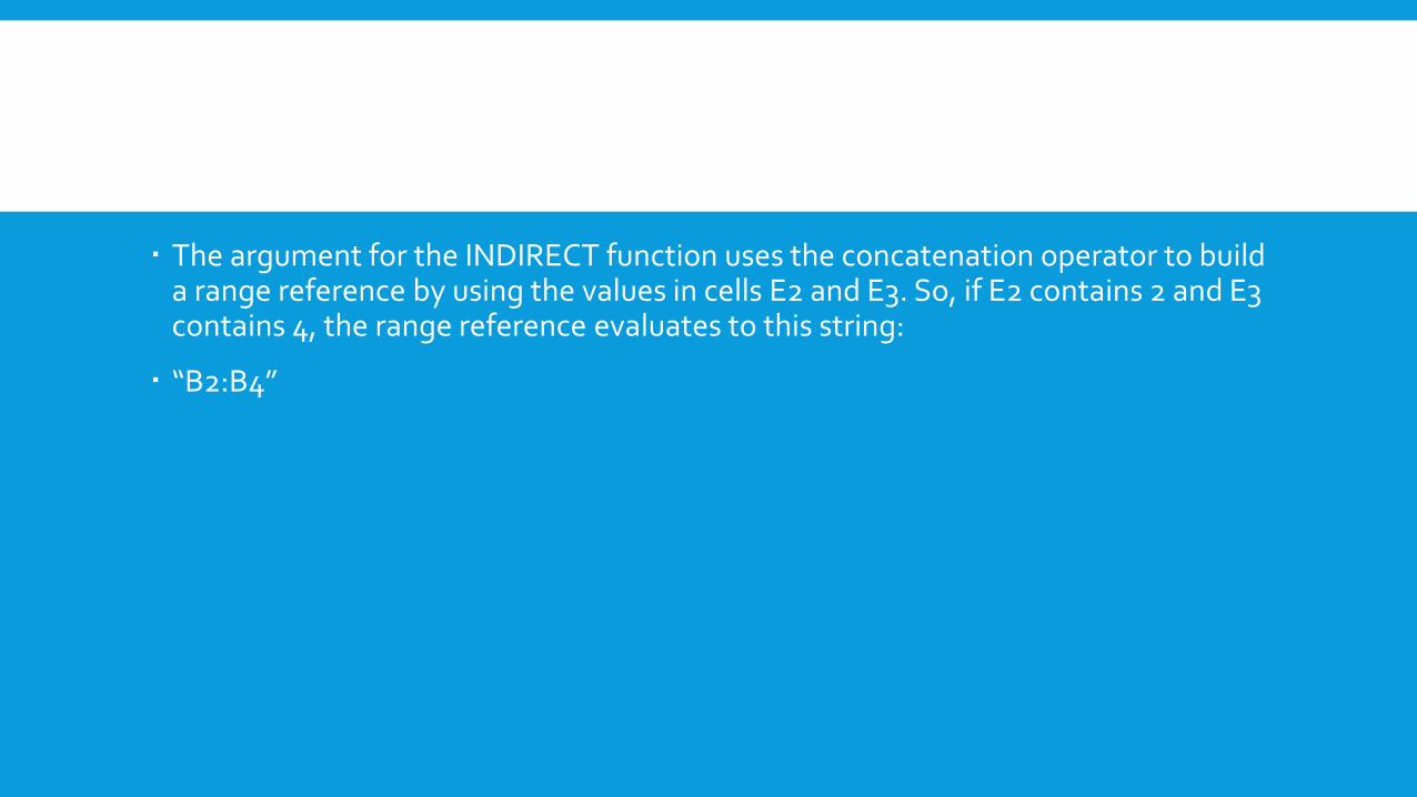
The argument for the INDIRECT function uses the concatenation operator to build a range reference by using the values in cells E2 and E3. So, if E2 contains 2 and E3 contains 4, the range reference evaluates to this string:

“B2:B4”

The INDIRECT function converts that string to an actual range reference, which is then passed to the

SUM function. In effect, the formula returns

=SUM(B2:B4)

When you change the values in E2 or E3, the formula is updated to display the sum of the specified rows.

SPECIFYING WORKSHEET NAMES INDIRECTLY

Column A, on the Summary worksheet, contains text that corresponds to other worksheets in the

workbook. Column B contains formulas that reference these text items. For example, the formula in

cell B2 is

=SUM(INDIRECT(A2&”!F1:F10”))

This formula concatenates the text in A2 with a range reference. The INDIRECT function evaluates the

result and converts it to an actual range reference. The result is equivalent to this formula:

=SUM(North!F1:F10)

This formula is copied down the column. Each formula returns the sum of range F1:F10 on the corresponding

worksheet.

Making a cell reference unchangeable

Another use for the INDIRECT function is to create a reference to a cell that never changes. For example,

consider this formula, which sums the values in the first 12 rows of column A:

=SUM(A1:A12)

If you insert a new row 1, Excel changes the formula to

=SUM(A2:A13)

In other words, the formula adjusts so that it continues to refer to the original data (and it no longer

sums the first 12 rows of column A). To prevent Excel from changing the cell references, use the

INDIRECT function:

=SUM(INDIRECT(“A1:A12”))

This formula always returns the sum of the first 12 rows in column A.

FORMULA EDITING IN DIALOG BOXES

This is a simple tip, but one that most users don’t know about.

When Excel displays a dialog box that accepts a range reference, the field that contains the range reference is always in point mode. For example, consider the New Name dialog box,This dialog box appears when you choose Formulas➜Defined Names➜Define Name.

If you activate the Refers to Field and use the arrow keys to edit the range reference, you’ll find that you’re actually pointing to a range in the worksheet —not editing the reference text. The solution:

Press F2.

The F2 key toggles between point mode and edit mode. In edit mode, the arrow keys work the same as when you’re editing a formula. Also notice that the current mode is displayed in the left corner of the status bar.

CONVERTING A VERTICAL RANGE TO A TABLE

You can convert this type of data several ways, but here’s a method that’s fairly easy. It uses a single

formula, which is copied to a range.

Enter the following formula in cell C1, and then copy it down and across.

=INDIRECT(“A” &COLUMN()-2 + (ROW()-1)*3)

The formula works for vertical data that uses three cells per record, but it can be modified to handle

vertical data that uses any number of cells per record by changing the “3” in the formula. For example,

if the vertical data has five fields, use this formula:

=INDIRECT(“A” &COLUMN()-2 + (ROW()-1)*5)

WORKING WITH DATA

Selecting Cells Efficiently

Many Excel users think that the only way to select a range of cells is to drag over the cells with the mouse. Although selecting cells with a mouse works, it’s rarely the most efficient way to accomplish the task. A better way is to use your keyboard to select ranges.

Selecting a range by using the Shift and arrow keys

The simplest way to select a range is to press (and hold) Shift and then use the arrow keys to highlight the cells. For larger selections, you can use PgDn or PgUpwhile pressing Shift to move in larger increments.

A RANGE OF CELLS.

Excel 2013

Education

Transcript of Excel 2013