3/23/2011

Excel 2010, Level IIIThank You For Attending The

COMPUTER TRAINING CENTERMore Computer Classes Available:

www.ConejoAdultSchool.org

Conejo Valley Adult School1025 Old Farm Road

Thousand Oaks, CA 91360

Excel 2010: Advanced

1. Logical and statistical functions

2. Financial and date functions

3. Lookups and data tables

4. Advanced data management

5. Exporting and importing

6. Analytical tools

7. Macros and custom functions

3/23/2011

The IF function

IF(logical_test,value_if_true,value_if_false)

AND, OR, and NOT functionsIF(AND(logical1, logical2),

value_if_true, value_if_false)

IF(OR(logical1, logical2),value_if_true, value_if_false)

IF(NOT(logical),value_if true, value_if_false)

3/23/2011

Nested IF functions • Use the nested IF function to evaluate multiple conditions

• Example: Use a second IF function as the value_if_false argument for the first IF function

The IFERROR function

IFERROR(value,value_if_error)

3/23/2011

The SUMIF function

SUMIF(range,criteria,sum_range)

The COUNTIF function

COUNTIF(range,criteria)

3/23/2011

The AVERAGEIF function

AVERAGEIF(range,criteria,average_range)

SUMIFS, COUNTIFS, AVERAGEIFS

SUMIFS(sum_range,criteria_range1,criteria1,criteria_range2,criteria2)

COUNTIFS(range1,criteria1,range2,criteria2)

AVERAGEIFS(average_range,criteria_range1,criteria1,criteria_range2,criteria2)

3/23/2011

The ROUND function

ROUND(value,num_digits)

Evaluate Formula dialog box

3/23/2011

The PMT function

PMT(rate,nper,pv,fv,type)

Date functions• Various built-in date functions can be used to insert dates

or perform date calculations

• To insert a date function:

– On the Formulas tab, in the Function Library group, click Date & Time and select the desired function

– Click the Insert Function button to open the Insert Function dialog box

3/23/2011

Calculating time• To find the difference between a start time and an end

time, use a basic subtraction formula=end_time-start_time

• Format the cell as Number or General to see the difference in hours

• If formatted as Time, the result will be displayed as hh:mm:ss

Array formulas• Syntax is the same as for any other Excel formula

• Start with = and use built-in functions

• Must press Ctrl+Shift+Enter to enter the array formula

• Array formulas are enclosed in braces: {}

• You cannot manually enter the braces to create an array formula

3/23/2011

Creating an array formula

Applying arrays to functions

3/23/2011

Modify an array formula1. Select the cell containing the array formula to be modified

2. Press F2

3. Edit the cell references as needed

4. Press Ctrl+Shift+Enter

Displaying formulas in cells• On the Formulas tab, click Show Formulas

• Press Ctrl +` (grave accent)

• When formulas are shown in the worksheet, they will print that way

3/23/2011

Hide formulas from users1. Select the cells whose formulas you want to hide2. On the Home tab, click Format and choose

Format Cells3. Click the Protection tab, check Hidden, and click

OK4. Click Format and choose Protect Sheet5. Ensure that “Protect worksheet and contents of

locked cells” is checked6. Click OK

Show hidden formulas1. On the Review tab, click Unprotect Sheet

2. Select the range of cells whose formulas you want to unhide

3. On the Home tab, click Format and choose Format Cells

4. Click the Protection tab, clear the Hidden checkbox, and click OK

3/23/2011

Automatic recalculation• Automatic recalculation in a large worksheet, with

numerous formulas, might be time-consuming and cumbersome

• Disable automatic recalculation in the Excel Options dialog box

– In the Formulas category, under Calculation, select Manual

• Press F9 or click Calculate Now to manually calculate formulas

Edit iteration calculation options

1. In the Excel Options dialog box, select Formulas

2. Under Calculation, check “Enable iterative calculation”

3. Specify the maximum number of iterations allowed

4. Specify the acceptable amount of change between calculations

5. Click OK

3/23/2011

The HLOOKUP function

HLOOKUP(lookup_value,table_array,row_index_num,range_lookup)

The VLOOKUP function

VLOOKUP(lookup_value, table_array,col_index_num,range_lookup)

3/23/2011

VLOOKUP for exact matches• Lookup value must always be in first column of lookup table

• If range_lookup argument is TRUE (exact match), values in first column of lookup range must be in ascending order

• Uppercase and lowercase text are equivalent

VLOOKUP for approximate matches

• Specify the range_lookup argument as TRUE

• If the function doesn’t find an exact match, it looks for the largest value that is less than the lookup value

• If the lookup value is less than the smallest value in the table, an error (#N/A) is returned

3/23/2011

HLOOKUP for exact matches• Lookup value must always be in first row of lookup table

• If range_lookup argument is TRUE, values in first row of lookup range must be in ascending order

• Uppercase and lowercase text are equivalent

HLOOKUP for approximate matches• Specify range_lookup argument as TRUE

• If the function doesn’t find an exact match, it looks for the largest value that is less than the lookup value, and returns its corresponding data

• If the lookup value is less than the smallest value in the table, an error (#N/A) is returned

3/23/2011

The MATCH function

MATCH(lookup_value,lookup_array,match_type)

The INDEX function

INDEX(range,row_num,col_num)

3/23/2011

One-variable data tables

Formula (in the row above the first input value and one column to the right of the input values)

Input values

Two-variable data tables

PMT function

Row input values (to the right of the formula)

Column input values (below the formula)

3/23/2011

Data validation• Ensures that the entered data matches a specified format

• Displays an input message that prompts users for correct entries

• Displays a specific error message when incorrect data is entered

• Circles invalid entries in the worksheet

Set data validation rules1. Select the cells for which you want to create a

validation rule2. On the Data tab, click Data Validation3. Click the Settings tab4. Select a data validation option5. Select the operator and complete the remaining

entries6. Enter a message to prompt users7. Enter a message for when invalid data is entered8. Click OK

3/23/2011

Use date criteria1. Select the cells you want to validate

2. Click Data Validation

3. From the Allow list, select Date

4. From the Data list, select the operator

5. Complete the remaining criteria entries

6. Define input and error messages

7. Click OK

Structure of database functionsDfunction(database,field,

criteria)

• database — Range containing the list of related information

• field — Column to be used by the function

• criteria — Range that contains the conditions a row must meet to be included in the calculation

3/23/2011

DSUM and DAVERAGEDSUM(database,field,criteria)

• Adds only the values in a database column that meet specific criteria

DAVERAGE(database,field,criteria)

• Calculates the average of values in a database column that meet specific criteria

Using the Save As command• Use Save As to export Excel data in other file

formats

– Some original formatting might be lost

• Commonly used formats:

– Text (Tab delimited)

– XML Paper Specification (XPS)

– Portable Document Format (PDF)

– Open Document Spreadsheet (ODS)

3/23/2011

Import data1. In the Open dialog box, specify the type of file you want to

import

2. Select the file

3. Click Open

The Text Import Wizard

3/23/2011

Converting text to columns

Removing duplicates

3/23/2011

The XML Maps dialog box

The XML Source pane

3/23/2011

Import XML data1. Click the Developer tab

2. In the XML group, click Import

3. Select the XML file containing the data

– Use the Address bar to find the file

4. Click Import

– Values in the XML file appear in the corresponding cells in the workbook

Export data to an XML file• Click Export in the XML group on the Developer tab

– The workbook should contain a valid XML map

– Before exporting the worksheet data, Excel will validate it against the map

3/23/2011

Delete an XML map1. In the XML Source pane, click XML Maps

2. Select the XML map you want to delete

3. Click Delete

– A message warns that you won’t be able to import or export XML data by using the XML map; click OK

4. Click OK

Use Microsoft Query1. Click the Data tab

2. Click From Other Sources and choose From Microsoft Query

3. Select <New Data Source> and click OK; specify the data-source name and select a driver; click Connect

4. Click Select to open the Select Database dialog box; select the source database; click OK twice

continued

3/23/2011

Use Microsoft Query, continued5. Select the data source and click OK; add the

desired tables and fields; click Next.

6. Specify the conditions you want the data to meet; click Next

7. Specify the sort order; click Next

8. Select Return Data to Microsoft Office Excel; click Finish

9. Specify whether to place the data in the existing worksheet or a new worksheet

10. Click OK

Web queries• To analyze data on the Web, such as online currency rates

or stock quotes, use a Web query

• When you run a Web query, Excel retrieves data that has been formatted with HTML or XML

3/23/2011

Retrieve data from a Web page1. On the Data tab, click From Web

2. Specify the address of the Web page containing the data you want to retrieve

3. Click the arrow next to the table you want to select

4. Click Options; select a format; click OK

5. Click Import; specify an existing or new worksheet; click OK

Use the Goal Seek utility 1. Click the Data tab

2. Click What-If Analysis and choose Goal Seek

3. Specify the cell that contains the formula you want to solve

4. Enter the result you want

5. Specify the cell that contains the value you want to adjust

6. Click OK

3/23/2011

Activate add-ins1. Open the Excel Options dialog box

2. In the category list, select Add-Ins

3. From the Manage list, select Excel Add-ins, and click Go

4. Check the add-ins you want to activate, and click OK

Excel add-ins are automatically installed with Office Tools; if you haven’t installed Office Tools yet, you must do so now

The Add-Ins dialog box

3/23/2011

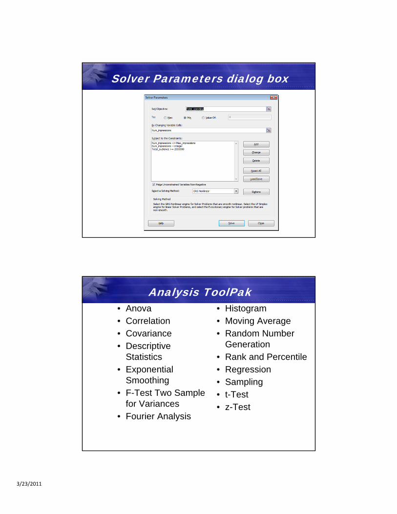
Solver Parameters dialog box

Analysis ToolPak• Anova• Correlation• Covariance• Descriptive

Statistics• Exponential

Smoothing• F-Test Two Sample

for Variances• Fourier Analysis

• Histogram• Moving Average• Random Number

Generation• Rank and Percentile• Regression• Sampling• t-Test• z-Test

3/23/2011

Use the Sampling analysis tool1. Click the Data tab

2. In the Analysis group, click Data Analysis

3. Select Sampling and click OK

4. Specify the range of data from which you want to select samples

5. Specify a sampling method and an output option

6. Click OK

Create a scenario1. Click the Data tab

2. From the What-If Analysis list, select Scenario Manager

3. Click the Add button

4. Specify the name of the scenario

5. Specify the cells containing the values you want to change, and click OK

6. Specify values for the changing cells, and click OK

3/23/2011

Add a Scenario Manager button

1. Open the Excel Options dialog box, and select Quick Access Toolbar

2. From the “Choose commands from” list, select Data tab

3. In the list of commands, select Scenario Manager, and click Add

4. Click OK

Merge scenarios1. Click the worksheet where you want to merge scenarios

2. Open the Scenario Manager dialog box

3. Click Merge

4. Select the worksheet that contains the scenarios you want to merge

5. Click OK

3/23/2011

A sample Scenario Summary

Run a macro1. Click the Developer tab

2. In the Code group, click Macros to open the Macro dialog box

3. Select the desired macro and click Run

3/23/2011

Record a macro1. Click the Record Macro button

2. Enter a macro name and shortcut key

– Macro names must begin with a letter and cannot contain spaces

– Macro names can include letters, numbers, and underscores

3. Click OK to start recording the macro

4. Perform the actions you want to include in the macro

5. Click the Stop Recording button

Assign macros to command buttons

1. Click Customize Quick Access Toolbar and choose More Commands

2. From the “Choose commands from” list, select Macros

3. Select the desired macro and click Add

4. Click OK

3/23/2011

Add macro buttons to the Ribbon

1. Right-click the Ribbon and choose Customize the Ribbon

2. From the “Choose commands from” list, select Macros

3. Under Main Tabs, select the Developer tab and click New Group

4. Click Rename and enter a new name for the group5. From the macro list, select the macro you want to

add, and click Add6. Click OK

Insert a button1. On the Developer tab, in the Controls group, click Insert

2. From the Form Controls menu, choose Button (Form Control)

3. In the worksheet, drag to draw the button

4. When the Assign Macro dialog box opens, select the macro

5. Click OK

3/23/2011

Change button propertiesRight-click the button and:

• Choose Edit Text to change the button text

• Choose Assign Macro to change the assigned macro

• Choose Format Control to change the control properties

Create an Auto_Open macro1. On the Developer tab, click Record Macro

2. In the Name box, enter Auto_Open

3. Select the desired location

4. Enter a description and click OK

5. Perform the steps you want the macro to record

6. Click Stop Recording

7. Save and close the workbook

3/23/2011

VBA code• Stored in sheets called modules

– Module — Might contain one or more sub procedures

– Sub procedure — A named block of lines of code that perform a sequence of steps

• VBA code consists of statements and comments

– Statements — Instructions that perform certain actions

– Comments — Text used to describe a section of code

Observe VBA code1. Open the Macro dialog box

2. Click Edit to open the Microsoft Visual Basic window

3. Choose File, Close and Return to Microsoft Excel

3/23/2011

Example of editing VBA code• You might have a macro that calculates the monthly

deduction at an interest rate of 12%

• You want to change the interest rate to 11%

• Instead of recording a new macro, you can edit the macro’s VBA code to reflect the new interest rate

Function procedures• Function procedure — Similar to sub procedure, but returns

a value on execution

• Built-in Excel functions, such as SUM and AVERAGE, are written with function procedures

• You can create custom functions

3/23/2011

Creating a custom functionSyntax

Function function name (arguments)Return valueEnd function

ExampleFunction Profit(sales, cost)Profit=sales-costEnd function