Maria Glymour Department of Society, Human Development and Health

Harvard School of Public Health mglymour@hsph.harvard.edu

SPER Conference

June 25, 2012 1

Examples of Instrumental Variable Analyses

Outline

06-25-2012 Session 2.2 Findings Instruments 2

• Finding an instrumental variable • IVs in randomized trials: Moving To Opportunity • Answering a parallel question with a natural experiment (lottery) • IVs from natural experiments: compulsory schooling law changes • IVs from genes: FTO as an IV for maternal obesity

• Goals:

1. Recognize contexts in which IV analyses might be feasible and useful

2. Recognize the limitations and assumptions of the IV analysis

3

How do you find an Instrumental Variable? 1. Randomize 2. Some other possible sources of exogenous variation:

a. Geography of city b. Policy variations c. Institutional features (banking policies, loan guarantees) d. Timing of newly available resources e. Wait lists or lotteries for subsidies f. Genetic polymorphisms

Randomizing is generally preferable, because the IV assumptions are more plausible and the 1st stage effects

are often larger.

Example 1, Moving To Opportunity Trial Families with children in urban public housing developments invited and randomized

to: Control section 8, or “low poverty” section 8 (must move to neighborhood with <10% poverty)

Once randomized: 60% of section 8 group moved 47% of low poverty group moved.

This may sound bad, but compare to a drug-based trials: Women’s Health Initiative: “At the time the trial was stopped, 54.0% of study

participants assigned to receive CEE and 53.5% of those assigned to receive placebo had discontinued use of their study medication.” –Hsia 2006

TODAY: “Adherence to the medication regimen before the primary outcome was reached or the study was completed ranged from 84% at month 8 to 57% at month 60” -TODAY study group, NEJM 2012

4

Example 1, Moving To Opportunity

5

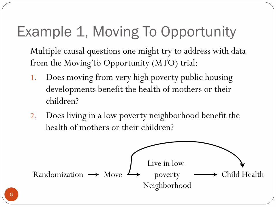
Multiple causal questions one might try to address with data from the Moving To Opportunity (MTO) trial:

1. Does moving from very high poverty public housing

developments benefit the health of mothers or their children?

2. Does living in a low poverty neighborhood benefit the health of mothers or their children?

Move Child Health Randomization Live in low-

poverty Neighborhood

Example 1, Moving To Opportunity

6

Multiple causal questions one might try to address with data from the Moving To Opportunity (MTO) trial: 1. Does moving from very high poverty public housing

developments benefit the health of mothers or their children?

2. Does living in a low poverty neighborhood benefit the health of mothers or their children?

Move Child Health Randomization Live in low-

poverty Neighborhood

Design Families with children in urban public housing developments

invited and randomized to: Control section 8, or “low poverty” section 8

Once randomized: 60% of section 8 group moved 47% of low poverty group moved.

This is the “first stage” estimate if you think of moving from

the development as the endogenous variable. 7

Did the trial affect neighborhood environment?

8 From ludwig 2011

This is the “first stage” estimate if you think of neighborhood poverty as the endogenous variable.

Poverty Rate Control ITT (Low Poverty) Mean Difference P-value

Baseline 53.1% -0.4 0.41

At 1 Year 50.0% -17.1 <.001

At 5 Years 39.9% -9.9 <.001

At 10 Years 33.0% -4.9 <.0001

IV analyses in MTO

9

• Standard 2-stage least squares • In most IV analyses, we think the “treated” group includes

some “always treated” people and some “compliers”. • The IV estimate refers to effect in the “complier” subgroup

who received treatment because of the value of the IV. • However, primary analyses of MTO define the endogenous

variable as moving from the development with the voucher given by the trial.

• In this definition of the treatment, it is impossible to be treated if you are not randomized to receive a voucher.

• Therefore, everyone who is “treated” is a “complier” and the IV effect estimate = effect of treatment on the treated (TOT)

Whose Causal Effect?

10

Never-Takers

Compliers

Contrarians/Defiers

Always Takers

Response if assigned to receive a voucher:

Don’t Move Move

Response if assigned to

not receive a voucher:

Mov

e D

on’t

Mov

e

10

Whose Causal Effect?

11

Never-Takers

Compliers

Contrarians/Defiers

Always Takers

Response if assigned to receive a voucher:

Don’t Move Move

Response if assigned to

not receive a voucher:

Mov

e D

on’t

Mov

e

11

Early Results for Behavioral Problems, Boston 2 Year Low Poverty Group vs Controls

12

Control Mean

ITT Difference (SE)

TOT/IV Difference (SE)

Boys .326 -.090 -.184

(.041) (.088)

Girls .193 -.023 -.046

(.030) (.056)

From Katz QJE 2001

Mid-Term (5-7 year) Results for Children’s Mental Health (K6)

13

Control Mean

ITT Difference (SE)

TOT/IV Difference (SE)

Boys -.162 .069 .167

(.091) (.223)

Girls .268 -.246 -.508

(.091) (.060)

Trial challenges

14

Mixed effects, attributable to Small samples? Heterogeneous effects?

Uncertainty about the salient component of the treatment Social disruption associated with moving? Changes in residential environment? Changes in schooling?

Who are the compliers?

Most of these issues arise whether you use IV or ITT to analyze the data

Example 1a:

Session 2.2 Findings Instruments 15

Causal question: Does moving from very high poverty public housing developments benefit the health of mothers or their children? We did a trial, but do you believe the results? Can we get more evidence? Voucher lottery

Jacob & Ludwig 2011

06-19-2012 Session 2.2 Findings Instruments 16

We match mortality data to information on every child in public housing that applied for a housing voucher in Chicago in 1997(N=11,848).

Families were randomly assigned to the voucher wait list, and only some families were offered vouchers.

Families randomized to the voucher moved to census tracts with an average of 7 points lower poverty.

Jacob & Ludwig 2011

06-19-2012 Session 2.2 Findings Instruments 17

Match mortality data to information on every child in public housing that applied for a housing voucher in Chicago in 1997(N=11,848).

Families were randomly assigned to the voucher wait list, and only some families were offered vouchers.

Jacob & Ludwig 2011

06-19-2012 Session 2.2 Findings Instruments 18

Match mortality data to information on every child in public housing that applied for a housing voucher in Chicago in 1997(N=11,848).

Families were randomly assigned to the voucher wait list, and only some families were offered vouchers.

Families randomized to the voucher moved to census tracts with an average of 7 points lower poverty.

Jacob & Ludwig 2011

06-19-2012 Session 2.2 Findings Instruments 19

Treatment group= children whose families were assigned a waitlist number from 1 to 18,110, and so were offered a voucher by May 2003

Control group = everyone assigned a higher lottery number. OLS with a person-quarter panel dataset for 1997:Q3 through

2005:Q4 yit measures child i’s outcome in quarter t, PostOfferit =1 if child

i’s family was offered a voucher prior to t, else PostOfferit = 0 X =control variables (whether the family is offered a voucher

some time after quarter t, gender, splines for baseline age (kinks at 1, 2, 5, 8 and 15) and calendar time (kinks every 6 calendar quarters). Clustered standard errors.

Jacob & Ludwig 2011

20

ITT:

IV:

IV analyses of a housing voucher lottery

06-19-2012 Session 2.2 Findings Instruments 21

ITT IV

Same analytic approach to natural experiment generated by a lottery and randomized experiment. Similar message re gender effect modification. Note large CIs.

Example 2, natural experiment based on policy change

06-19-2012 Session 2.2 Findings Instruments 22

Causal question: Does completing additional years of education improve memory in old age?

Substantive Question

Multiple studies show that years of education predicts old age cognitive function, cognitive change, and

dementia.

Causality questionable.

Childhood SES Childhood IQ

Personality

Years of schooling

Old Age Cognitive Outcomes

Natural Experiments for Education

Schooling Old Age Cognitive

Outcomes

Childhood SES Childhood IQ

Personality

?

Quarter of Birth, Compulsory School

Laws, School Term Length,

Kindergarten

Natural Experiments: UK Education Reform Effect on Education

From Banks and Mazzona, 2012 25

Natural Experiments: UK Education Reform Effect on Education

From Banks and Mazzona, 2012 26

Reform had a powerful and immediate effect on about half the population of 14 years olds.

Natural Experiments: IV Estimates for Education effect on EF

From Banks and Mazzona, 2012 27

Natural Experiments: IV Estimates for Education Effect on EF

From Banks and Mazzona, 2012 28

Note sensitivity to model for temporal trends.

Estimating the IV effect

29

Banks & Mazzona call this a “fuzzy regression discontinuity design” and estimate with 2SLS.

Males Females Year

band=1 Year

band=3 Year band=1 Year

band=3

Memory .60 (.35) .43 (.19) .51 (.34) .35 (.19)

Exec Fx .64 (.36) .37 (.19) -.10 (.39) .09 (.21)

IV Estimates Using US Policy Changes

06-19-2012 Session 2.2 Findings Instruments 30

Banks and Mazzona replicated earlier findings in the US Advantage of the US context: Education is decentralized, so there were more places that

changed policies Allows for better control of secular trends: you can rule out a

sudden change in 1947.

Disadvantage of the US context: Effect of the laws was very small Generally not well enforced, most people would have attended

more school than required anyway Complier group is small.

Early 20th Century CSL Changes

5

6

7

8

9

10

11

1909

1911

1913

1915

1917

1919

1921

1923

1925

1927

1929

1931

1933

1935

1937

1939

1941

1943

1945

1947

Com

puls

ory

Scho

ol

SC-CSL

IV Analyses State schooling policies Compulsory school to drop out (CSL) or receive a work-permit

(CSL-W) Based on policy in state of birth when school-age 2-Sample least squares analysis

Exposure (endogenous) variable: Years of education (self-report)

Data Set: 1st Stage

IPUMS (Census) 5% 1980 sample, Birth years 1900-1947 Years of education linked to CSLs and CSL-Ws based on state

of birth Link predictions from 1st stage regression model to individual

data in the 2nd stage based on state of birth and all covariates.

33

Data Set: 2nd stage

Health & Retirement Study, 1992-2000: panel enrollment by birth cohort (whites only due to evidence on enforcement)

Cognitive assessments and state of birth on 21,041

individuals born 1900-1947

CSLs and CSL-Ws

34

Two-Sample Least Squares

CSLs in each state and year, 1906-1961.

Sample 1: 5% Census sample.

Predicted education

(Ê).

Sample 2: HRS data.

Stage 1: Regress education on CSLs, with other covariates.

Stage 2: Regress health outcomes on Ê, with other stage 1 covariates. Regression coefficient for Ê is the IV effect estimate.

35

Covariates

Unadjusted

Sex Birthyear (indicators for every year)

State of birth indicators

State characteristics: age 6 % black, % urban, and % foreign born; age 14 manufacturing jobs per capita and wages per manufacturing job

1

2

3

4

36

Do the Instruments Predict Education?

1. Unadjusted Model

2. Birthyear and sex

3. Model 2 + state of birth

4. Model 3 + state condns

CSLs 0.238 0.110 0.062 0.037(0.236, 0.240) (0.108, 0.112) (0.059, 0.064) (0.034, 0.040)

CSL-Ws 0.143 -0.032 0.063 0.044(0.146, 0.141) (-0.034, -0.029) (0.060, 0.066) (0.040, 0.048)

CSL-Ws UNR -1.397 -0.282 -0.204 0.034(-1.429, -1.365) (-0.315, -0.249) (-0.238, -0.17) (0.000, 0.069)

First stage regression results (from IPUMS 5% sample)

37

How Strong is the 1st Stage?

β 95% CI β 95% CI β 95% CI β 95% CI

Model r2 without instrumental variables

Model r2 including instrumental variables

Variance explained by instrumental variables

4. Model 3 + state

characteristics#

2. Birthyear*

and sex.

3. Model 2 + state of birth

indicators

1. Unadjusted Model

0.0000

0.0465

0.0465

0.1626

0.1631

0.0005

0.1080

0.1127

0.0047

0.1599

0.1613

0.0014

Not technically “weak” instruments, but clear that a small violation of the IV assumptions could introduce a large amount of bias.

38

IV Estimates for Education: CSLs

Model covariates βIV 95% CI^ βIV 95% CI^

1. Unadjusted 0.33 (0.27, 0.39) 0.19 (0.12, 0.26)

2. Birthyear, and sex 0.30 (0.14, 0.46) 0.34 (0.05, 0.63)

3. Model 2 + birth state 0.18 (0.02, 0.33) 0.03 (-0.22, 0.27)

4. Model 3 + state condns 0.34 (0.11, 0.57) -0.06 (-0.37, 0.26)

Memory CognitionEstimated effect of 1 year ed’n on cognitive test scores.

5. OLS estimates 0.09 (0.08, 0.10) 0.15 (0.14, 0.16) 39

Evaluating Instruments Is the dependent variable independent of the instrument

conditional on the endogenous variable? Over-identification tests, if you have multiple instruments Inequality constraints (for categorical endogenous variables) Evaluate the association between the instrument and the

outcome across environments that modify the 1st stage association

40

Sensitivity Analyses Including education >13 years βIV (memory, model 3): 0.15 (-0.01, 0.31)

Restricting to education > 13 years Instruments do not predict education or memory for

individuals with >13 years of school βIV (memory, model 3): -1.04 (-3.70, 1.62)

Inverse probability weighted for missing Memory (parental SES, self-report chronic condns at baseline) βIV (memory, model 3): 0.19 (0.03, 0.36)

41

Example 3: Maternal FTO as an IV for effect of mom’s BMI on child’s BMI

42

Mom BMI During

Pregnancy

Child BMI

Mom FTO

Child FTO

42

Goal was to test developmental overnutrition hypothesis: exposure during gestation affects child BMI

IV effect estimates for Maternal BMI on Offspring total fat mass

06-19-2012 Session 2.2 Findings Instruments 43

OLS IV P-value for test of difference OLS vs IV

Total Fat Mass 0.26 (0.23, 0.29

-0.08 (-0.56, 0.41)

.17

From Lawlor PLoS Medicine 2008

Example 3: Maternal FTO as an IV for effect of mom’s BMI on child’s BMI

44

Mom BMI During

Pregnancy

Child BMI

Mom FTO

Child FTO

44

Mom’s Diet

Doubting Instruments Do they have other pathways to the outcome? Quarter of birth

Is there a common cause of the instrument and the outcome? State of birth

Do they actually affect anyone’s exposure? Tax policies

45

Thinking of Instruments, Creating Instruments

Often ecological Policy changes Policy discontinuities Differences in “expert” opinion Encouragement designs: randomize the incentive Ask: What is the process that determines exposure? Is

any part of this process arbitrary/random? Content matter experts are very valuable team members

46

Conclusions

Many important questions not convincingly answered with observational evidence

Abandon the difficult questions? Or learn what we can from fraught methods?

IV adds: A way forward with observational data Sometimes a parameter estimate of special interest Pushes us to identify interventions that change exposures

Not a replacement for evidence from observational research or RCTs, but a useful supplement

47

end

06-19-2012 Session 2.2 Findings Instruments 48