1

Exercise 4. Terrain Analysis12

Spring 2017

Prepared by Ayse Kilic - revised March 8, 2017

Goal

The goal of this exercise is to serve as an introduction to Spatial Analysis with ArcGIS.

Objectives Use surface and hydrology tools to calculate terrain attributes Use raster data and raster calculator functionality to calculate watershed attributes such as mean

elevation, mean annual precipitation and runoff ratio. Interpolate data values at points to create a spatial field to use in hydrologic calculations

Computer and Data Requirements

To carry out this exercise, you need to have a computer that runs ArcGIS for Desktop 10.3.0. The necessary data are provided in a zipped file (Exe4Data.zi) at the course web site:http://snr.unl.edu/kilic/gisrs/2017/

Readings

Handout on "Computation of Slope" at http://snr.unl.edu/kilic/gisrs/2017/Slope.pdf

1 The structure of this exercise originated from Dr. David Tarbon, Utah State University. 2 Assistance in organizing data sets used in this exercise and testing of ArcGIS applications was provided by Mr. Bhavnet Soni, Ph.D. Candidate, UNL.

2

Part 1 . Upper Klamath Lake ( U K L ) Elevation and Precipitation.

The purpose of this part of the exercise is to use a DEM to calculate average watershed elevation for subwatersheds of the Upper Klamath Lake (UKL) basin, and to calculate average precipitation over each of these subwatersheds using different interpolation methods. We will also use the terrain analysis model/toolbox that you developed in previous exercise (Flow Direction_from_Tiff) to calculate slopes and flow directions for the UKL.

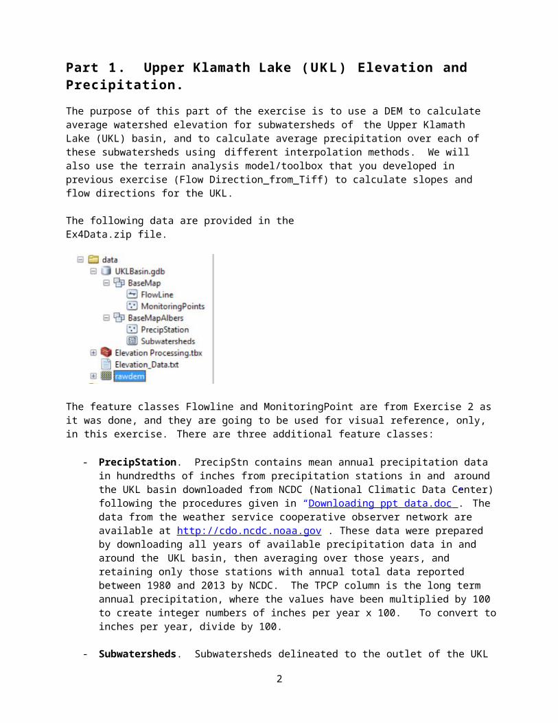
The following data are provided in the Ex4Data.zip file.

The feature classes Flowline and MonitoringPoint are from Exercise 2 as it was done, and they are going to be used for visual reference, only, in this exercise. There are three additional feature classes:

- PrecipStation. PrecipStn contains mean annual precipitation data in hundredths of inches from precipitation stations in and around the UKL basin downloaded from NCDC (National Climatic Data Center) following the procedures given in “Downloading ppt data.doc ” . The data from the weather service cooperative observer network are available at http://cdo.ncdc.noaa.gov . These data were prepared by downloading all years of available precipitation data in and around the UKL basin, then averaging over those years, and retaining only those stations with annual total data reported between 1980 and 2013 by NCDC. The TPCP column is the long term annual precipitation, where the values have been multiplied by 100 to create integer numbers of inches per year x 100. To convert to inches per year, divide by 100.

- Subwatersheds. Subwatersheds delineated to the outlet of the UKL as well as each of the stream gages in MonitoringPoint following the procedures that will be learned in a future exercise. The stream gages are reporting mean annual flow in cubic feet per second (cfs).

- RawDEM. A digital elevation model from the National Elevation dataset is provided in the feature named RawDEM.

The PrecipStation and subwatersheds feature classes are in a feature dataset named BaseMapAlbers as it works best to make area calculations for hydrologic analysis using an equal area projected coordinate system.

3

1. Loading the DataOpen ArcMap (blank document) and from the geodatabase UKLBasin.gdb (double click on it), add the contents of the BaseMapAlbers feature dataset to the map display (the PrecipStation and SubWatersheds feature classes). The following map should load showing the subwatersheds in green and the precipitation stations as black points.

If you right click on one of these two feature classes, you’ll see that this is the NAD_83_Albers map projection – an Albers Equal Area projection using the NAD 83 datum.

4

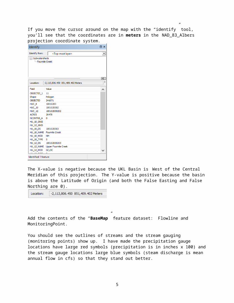
If you move the cursor around on the map with the “identify” tool, you’ll see that the coordinates are in meters in the NAD_83_Albers projection coordinate system.

The X-value is negative because the UKL Basin is West of the Central Meridian of this projection. The Y-value is positive because the basin is above the Latitude of Origin (and both the False Easting and False Northing are 0).

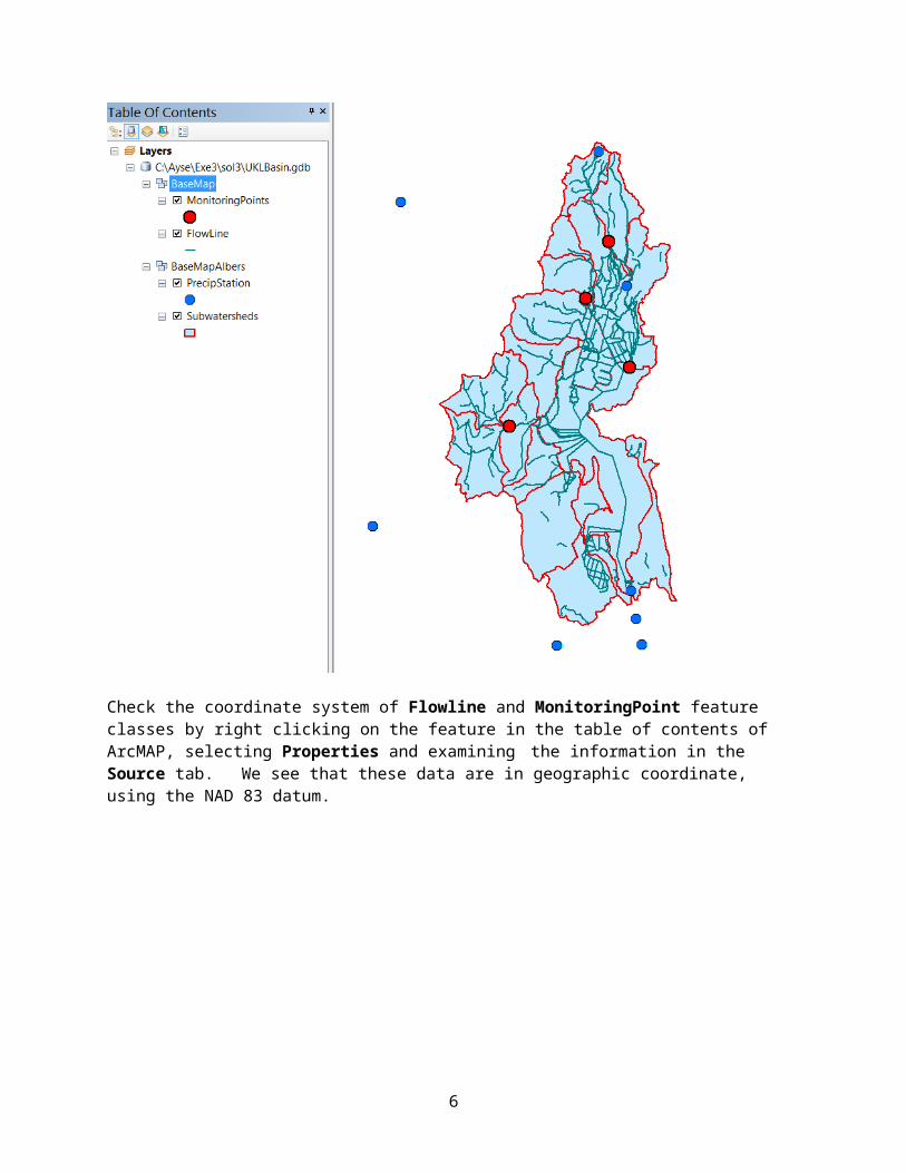
Add the contents of the “BaseMap” feature dataset: Flowline and MonitoringPoint.

You should see the outlines of streams and the stream gauging (monitoring points) show up. I have made the precipitation gauge locations have large red symbols (precipitation is in inches x 100) and the stream gauge locations large blue symbols (steam discharge is mean annual flow in cfs) so that they stand out better.

5

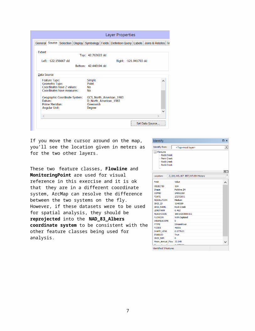
Check the coordinate system of Flowline and MonitoringPoint feature classes by right clicking on the feature in the table of contents of ArcMAP, selecting Properties and examining the information in the Source tab. We see that these data are in geographic coordinate, using the NAD 83 datum.

6

If you move the cursor around on the map, you’ll see the location given in meters as for the two other layers.

These two feature classes, Flowline and MonitoringPoint are used for visual reference in this exercise and it is ok that they are in a different coordinate system, ArcMap can resolve the difference between the two systems on the fly. However, if these datasets were to be used for spatial analysis, they should be reprojected into the NAD_83_Albers coordinate system to be consistent with the other feature classes being used for analysis.

7

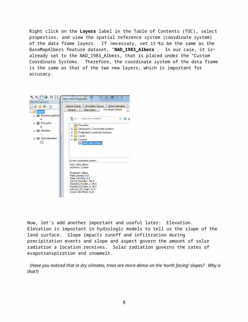
Right click on the Layers label in the Table of Contents (TOC), select properties, and view the spatial reference system (coordinate system) of the data frame layers. If necessary, set it to be the same as the BaseMapAlbers feature dataset, "NAD_1983_Albers”. In our case, it is already set to the NAD_1983_Albers, that is placed under the “Custom” Coordinate Systems. Therefore, the coordinate system of the data frame is the same as that of the two new layers, which is important for accuracy.

Now, let’s add another important and useful later: Elevation. Elevation is important in hydrologic models to tell us the slope of the land surface. Slope impacts runoff and infiltration during precipitation events and slope and aspect govern the amount of solar radiation a location receives. Solar radiation governs the rates of evapotranspiration and snowmelt.

(Have you noticed that in dry climates, trees are more dense on the ‘north facing’ slopes? Why is that?)

8

Add the grid Rawdem to ArcMap. This is a digital elevation model that was downloaded from the National Map viewer, http://viewer.nationalmap.gov/viewer/. DEMs generally come in small area frames depending up on the size of area and the resolution. For the purpose of this exercise we have mosaiced smaller DEMs into one single DEM for easier use. Your map should look similar to the following:

The DEM grid is skewed in this display because it was obtained in geographic coordinates. The legend informs us that the brighter tones indicate high elevations and darker tones indicate low elevations. Note (beneath the basin shape (you can turn subwatersheds off) that there are relatively high mountains in the west and northern parts of the UKL basin. Also note how the terrain slopes toward the west when moving west of our basin. That area is part of a different water basin. The Crater Lake National Park is visible in the north of the UKL basin. Crater Lake is an extinct volcano with a large lake in the crater. The UKL originates at the southern rim of the volcano.

9

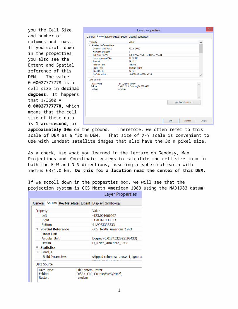
Let’s investigate whether the DEM is in the same coordinate system as our other layers. Right click on the rawdem layer in the table of contents and select properties. Click on the Source tab. This shows you the Cell Size and number of columns and rows. If you scroll down in the properties you also see the Extent and Spatial reference of this DEM. The value 0.00027777778 is a cell size in decimal degrees. It happens that 1/3600 = 0.00027777778, which means that the cell size of these data is 1 arc-second, or approximately 30m on the ground. Therefore, we often refer to this scale of DEM as a “30 m DEM.” That size of X-Y scale is convenient to use with Landsat satellite images that also have the 30 m pixel size.

As a check, use what you learned in the lecture on Geodesy, Map Projections and Coordinate systems to calculate the cell size in m in both the E-W and N-S directions, assuming a spherical earth with radius 6371.0 km. Do this for a location near the center of this DEM.

If we scroll down in the properties box, we will see that the projection system is GCS_North_American_1983 using the NAD1983 datum:

To turn in: A snapshot of your screen showing the five data layers; a table showing the number of columns and rows, cell size in the E-W and N-S directions in m, extent (in degrees) and spatial reference information for the UKL elevation dataset 'Rawdem'.

10

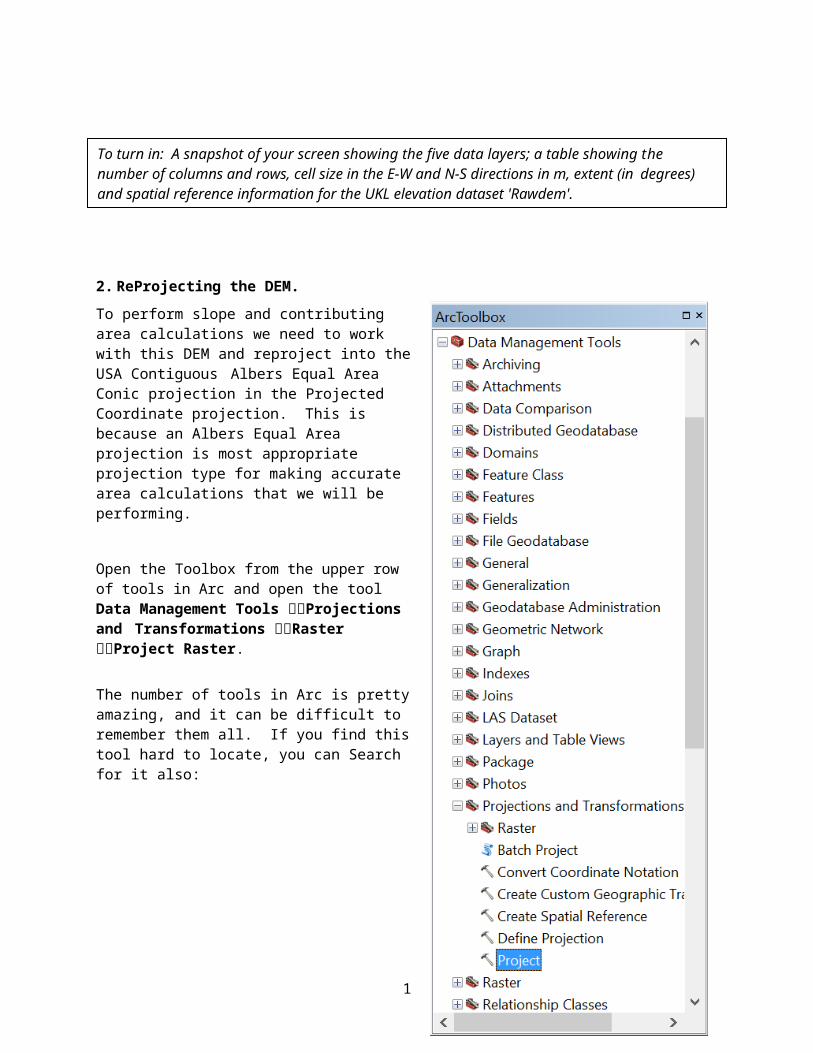
2. ReProjecting the DEM.To perform slope and contributing area calculations we need to work with this DEM and reproject into the USA Contiguous Albers Equal Area Conic projection in the Projected Coordinate projection. This is because an Albers Equal Area projection is most appropriate projection type for making accurate area calculations that we will be performing.

Open the Toolbox from the upper row of tools in Arc and open the tool Data Management Tools Projections and Transformations Raster Project Raster.

The number of tools in Arc is pretty amazing, and it can be difficult to remember them all. If you find this tool hard to locate, you can Search for it also:

11

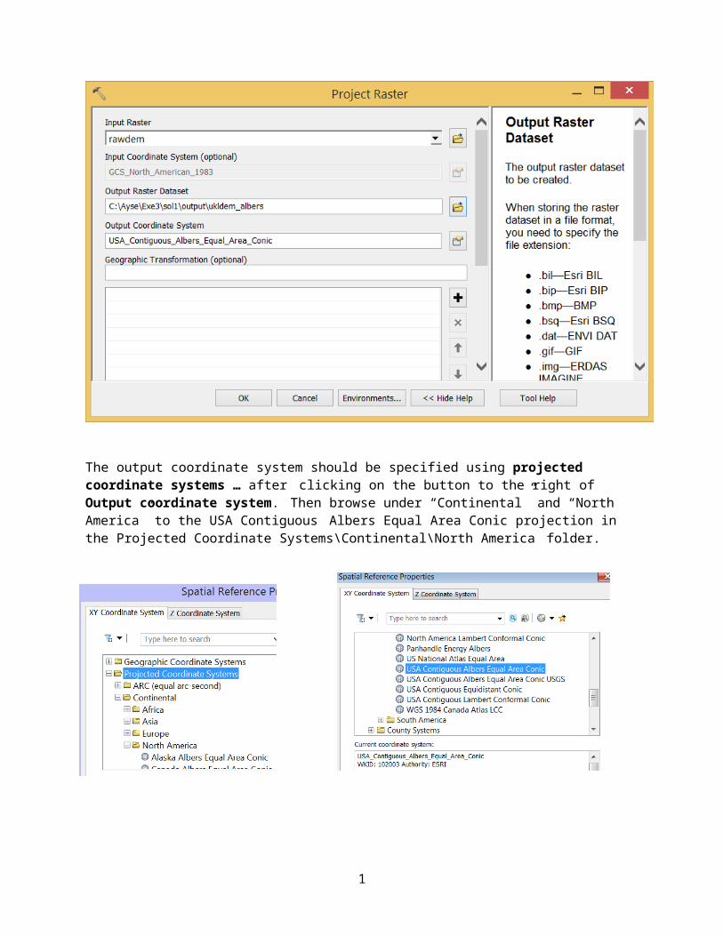
Set the inputs as follows:

The output coordinate system should be specified using projected coordinate systems … after clicking on the button to the right of Output coordinate system. Then browse under “Continental” and “North America” to the USA Contiguous Albers Equal Area Conic projection in the Projected Coordinate Systems\Continental\North America folder.

12

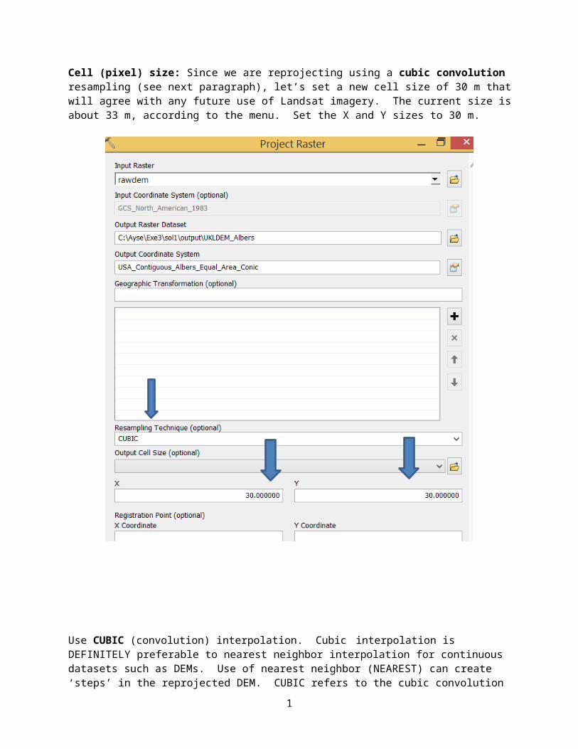
Cell (pixel) size: Since we are reprojecting using a cubic convolution resampling (see next paragraph), let’s set a new cell size of 30 m that will agree with any future use of Landsat imagery. The current size is about 33 m, according to the menu. Set the X and Y sizes to 30 m.

Use CUBIC (convolution) interpolation. Cubic interpolation is DEFINITELY preferable to nearest neighbor interpolation for continuous datasets such as DEMs. Use of nearest neighbor (NEAREST) can create ‘steps’ in the reprojected DEM. CUBIC refers to the cubic convolution method that determines the new cell value by fitting a smooth curved surface through the surrounding points using a predefined weighting function. This works best for a continuous surface like topography. The NEAREST neighbor resampling method simply grabs the value for the ‘old pixel’ that lies closest to the center location of the reprojected pixel. That can cause some ‘old pixel’ values to be used for two or more ‘new pixels’, creating a ‘plateau’ of elevation. That causes problems later in calculating slope, and can cause artificial "striping" that can appear in a shaded relief map (we will construct a shaded relief map below).

Click "OK" to invoke the tool. After the process is complete, the projected DEM, UKLDEM_albers, is added to ArcMap.

13

Examine the properties of the projected dataset. You should now have TWO DEM layers. The original “RawDEM” layer and the reprojected layer. Before you remove the RawDEM layer, turn off and on and off and on the reprojected (UKLDEM_albers) layer to expose the original RawDEM layer to insure that they are ‘identical.’ In actuality, if you were to zoom in closely, you would see differences caused by the resampling and the resizing to 30 m. Answer the questions in the box below.

You can now remove the RawDEM layer. It has served its purpose

3. Exploring the DEMThe spatial information about the DEM can be found by right clicking on the UKLDEM_albers layer, then clicking on PropertiesSource. This will confirm the 30 m size for X and Y rasters and the projection system.

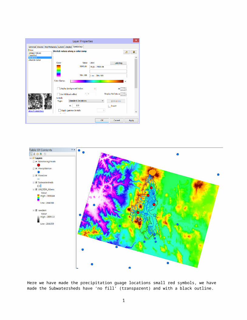
Similarly, the symbology of the DEM can be changed by right clicking on the layer, PropertiesSymbology. This is useful for adding some color to the feature graphic. For example, select the “Color Ramp” drop down and select a new color scheme. For example:

To turn in: The number of columns and rows in the reprojected DEM. The minimum and maximum elevations in the projected DEM. Explain why the minimum and maximum elevations are different from the minimum and maximum elevations in the original DEM.

14

Here we have made the precipitation guage locations small red symbols, we have made the Subwatersheds have ‘no fill’ (transparent) and with a black outline.

15

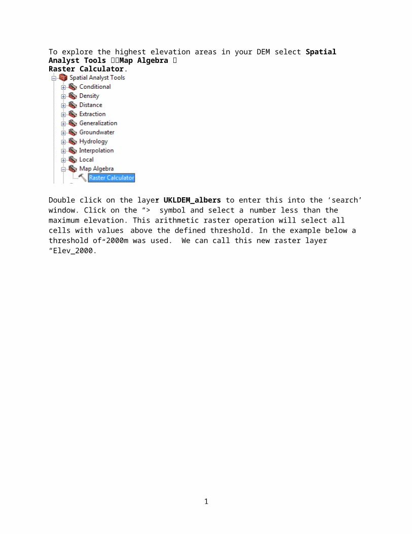
To explore the highest elevation areas in your DEM select Spatial Analyst Tools Map Algebra Raster Calculator.

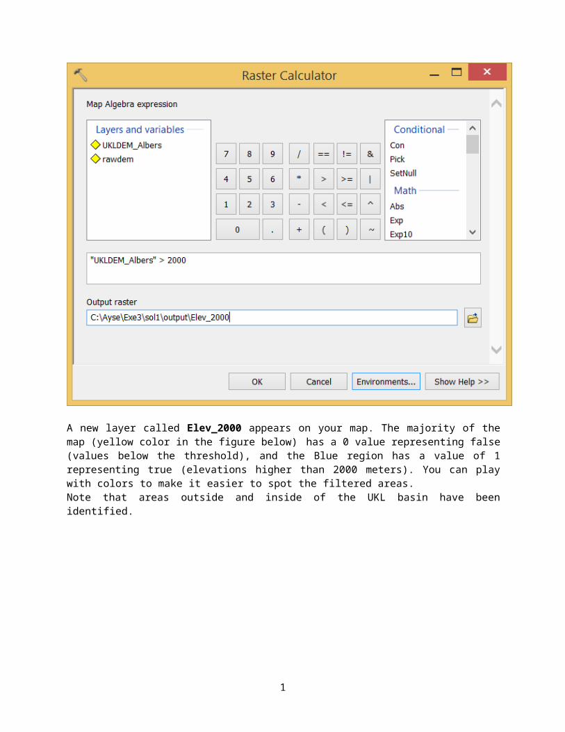
Double click on the layer UKLDEM_albers to enter this into the ‘search’ window. Click on the “>” symbol and select a number less than the maximum elevation. This arithmetic raster operation will select all cells with values above the defined threshold. In the example below a threshold of 2000m was used. We can call this new raster layer “Elev_2000.”

A new layer called Elev_2000 appears on your map. The majority of the map (yellow color in the figure

16

below) has a 0 value representing false (values below the threshold), and the Blue region has a value of 1 representing true (elevations higher than 2000 meters). You can play with colors to make it easier to spot the filtered areas.Note that areas outside and inside of the UKL basin have been identified.

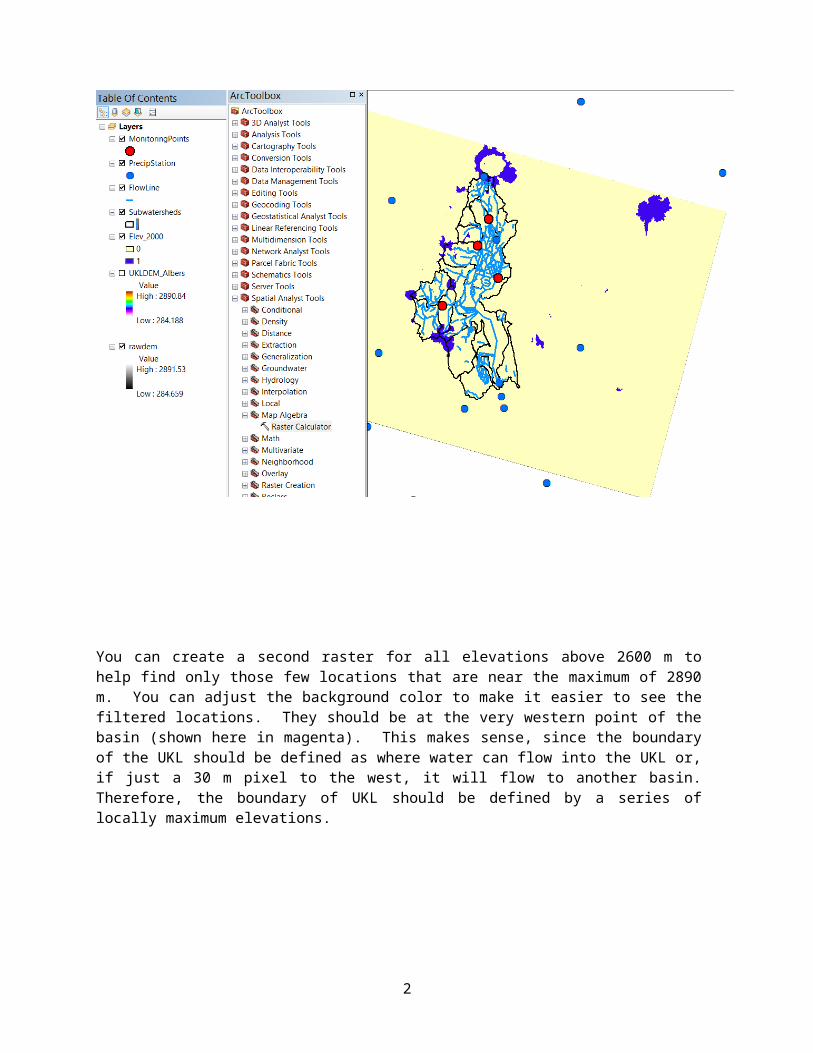
You can create a second raster for all elevations above 2600 m to help find only those few locations that are near the maximum of 2890 m. You can adjust the background color to make it easier to see the filtered locations. They should be at the very western point of the basin (shown here in magenta). This makes sense, since the boundary of the UKL should be defined as where water can flow into the UKL or, if just a 30 m pixel to the west, it will flow to another basin. Therefore, the boundary of UKL should be defined by a series of locally maximum elevations.

17

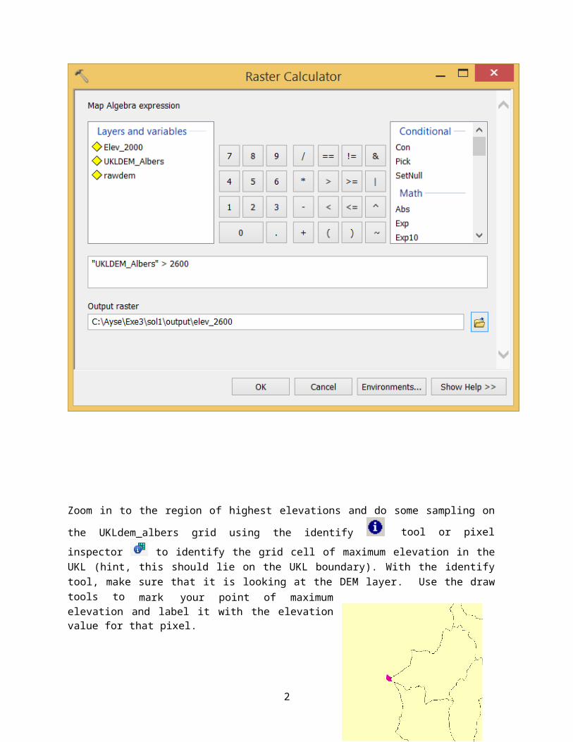
Zoom in to the region of highest elevations and do some sampling on the UKLdem_albers grid using

the identify tool or pixel inspector to identify the grid cell of maximum elevation in the UKL (hint, this should lie on the UKL boundary). With the identify tool, make sure that it is looking at the DEM layer. Use the draw tools to mark your point of maximum elevation and label it with the elevation value for that pixel.

18

4. Using our Custom Flow Direction tool with the UKL DEM

Now that we have reprojected the DEM for our study area, let’s use the Flow Direction tool that we created earlier, and modified to use a TIF file as input.

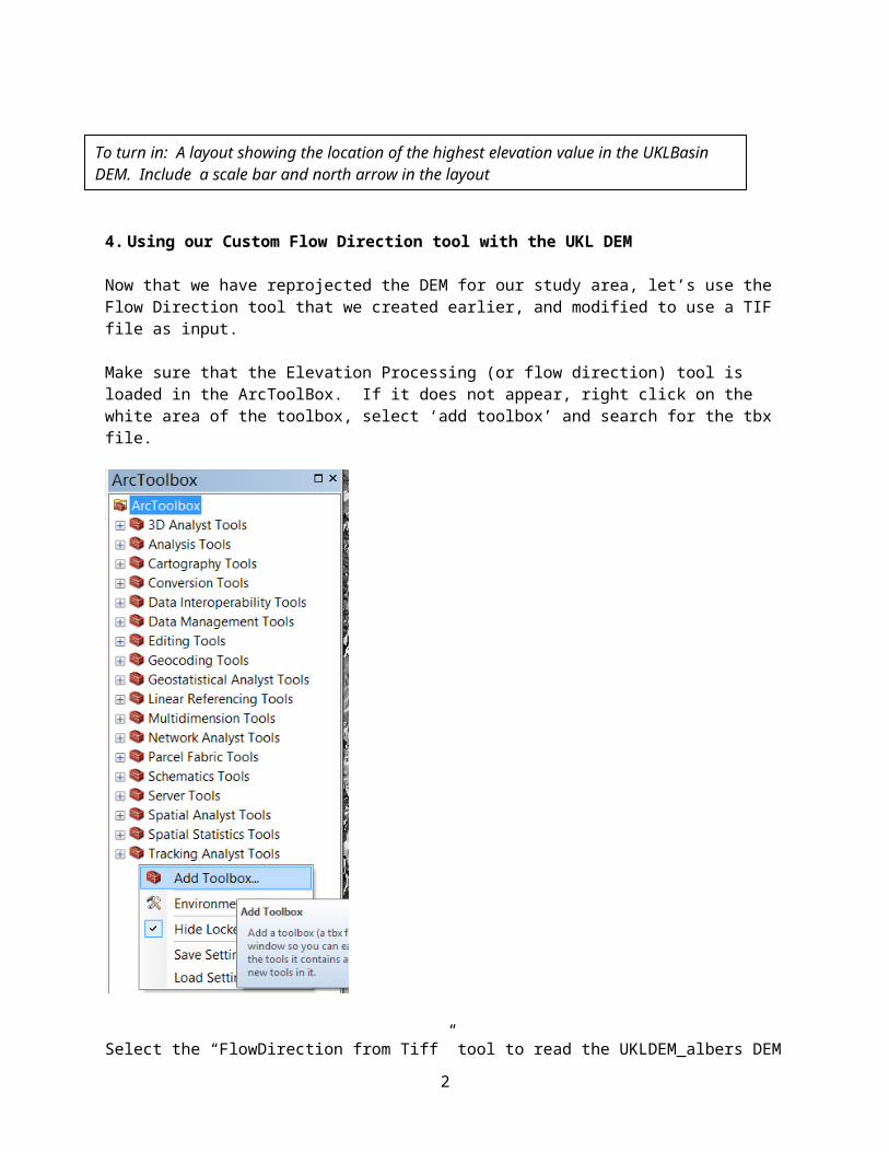
Make sure that the Elevation Processing (or flow direction) tool is loaded in the ArcToolBox. If it does not appear, right click on the white area of the toolbox, select ‘add toolbox’ and search for the tbx file.

To turn in: A layout showing the location of the highest elevation value in the UKLBasin DEM. Include a scale bar and north arrow in the layout

19

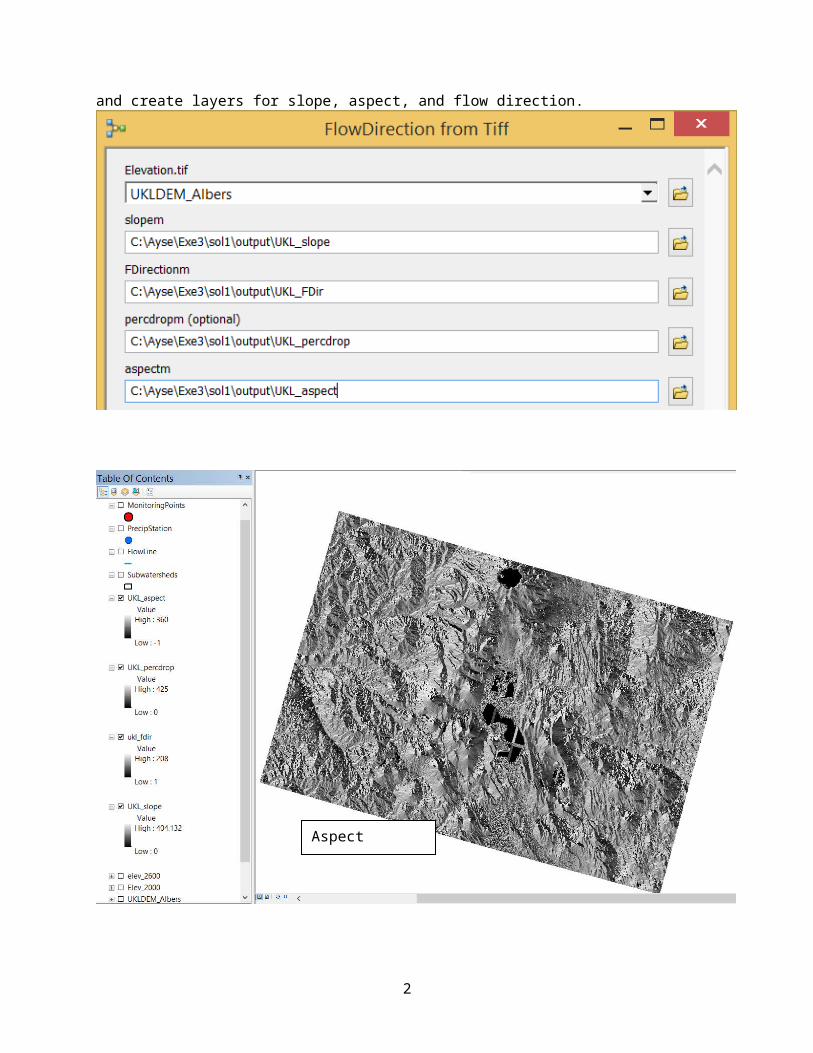
Select the “FlowDirection from Tiff” tool to read the UKLDEM_albers DEM and create layers for slope, aspect, and flow direction.

20

You should create the output layers in the same folder as your exercise 3.

Press OK, and wait a few minutes for the tool to process the entire DEM file. If successful, you should see a window like that to the right, after all four model components have run.

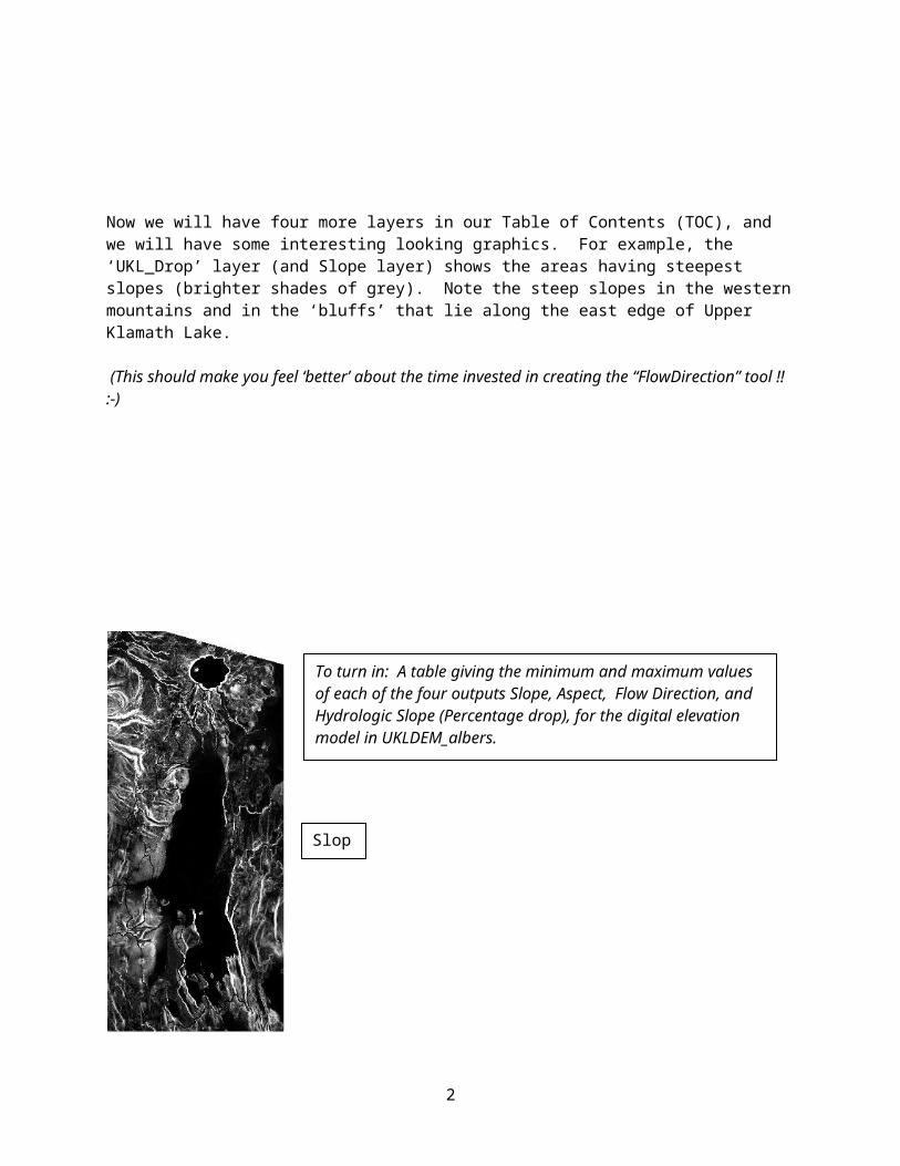
Now we will have four more layers in our Table of Contents (TOC), and we will have some interesting looking graphics. For example, the ‘UKL_Drop’ layer (and Slope layer) shows the areas having steepest slopes (brighter shades of grey). Note the steep slopes in the western mountains and in the ‘bluffs’ that lie along the east edge of Upper Klamath Lake.

(This should make you feel ‘better’ about the time invested in creating the “FlowDirection” tool !! :-)

Slope

To turn in: A table giving the minimum and maximum values of each of the four outputs Slope, Aspect, Flow Direction, and Hydrologic Slope (Percentage drop), for the digital elevation model in UKLDEM_albers.

Aspect

21

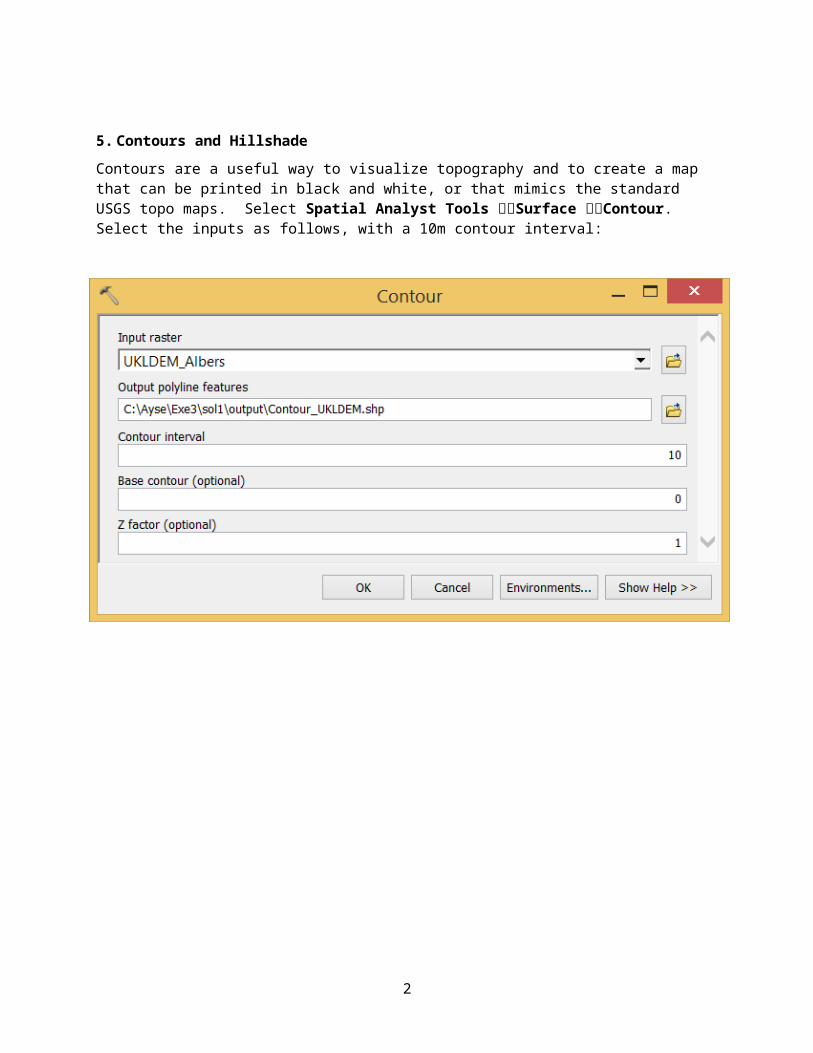
5. Contours and HillshadeContours are a useful way to visualize topography and to create a map that can be printed in black and white, or that mimics the standard USGS topo maps. Select Spatial Analyst Tools Surface Contour. Select the inputs as follows, with a 10m contour interval:

22

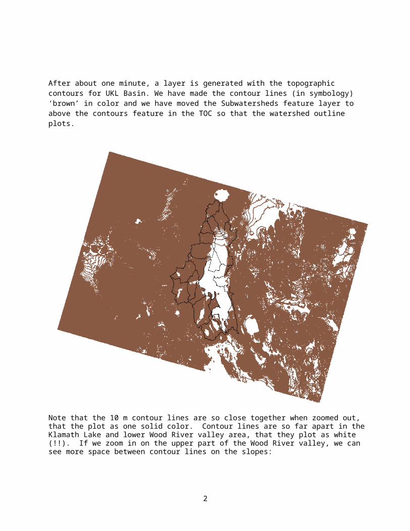
After about one minute, a layer is generated with the topographic contours for UKL Basin. We have made the contour lines (in symbology) ‘brown’ in color and we have moved the Subwatersheds feature layer to above the contours feature in the TOC so that the watershed outline plots.

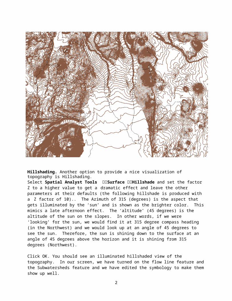
Note that the 10 m contour lines are so close together when zoomed out, that the plot as one solid color. Contour lines are so far apart in the Klamath Lake and lower Wood River valley area, that they plot as white (!!). If we zoom in on the upper part of the Wood River valley, we can see more space between contour lines on the slopes:

23

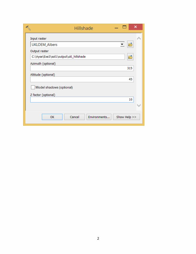
Hillshading. Another option to provide a nice visualization of topography is Hillshading.Select Spatial Analyst Tools Surface Hillshade and set the factor Z to a higher value to get a dramatic effect and leave the other parameters at their defaults (the following hillshade is produced with a Z factor of 10).. The Azimuth of 315 (degrees) is the aspect that gets illuminated by the ‘sun’ and is shown as the brighter color. This mimics a late afternoon effect. The ‘altitude’ (45 degrees) is the altitude of the sun on the slopes. In other words, if we were ‘looking’ for the sun, we would find it at 315 degree compass heading (in the Northwest) and we would look up at an angle of 45 degrees to see the sun. Therefore, the sun is shining down to the surface at an angle of 45 degrees above the horizon and it is shining from 315 degrees (Northwest).

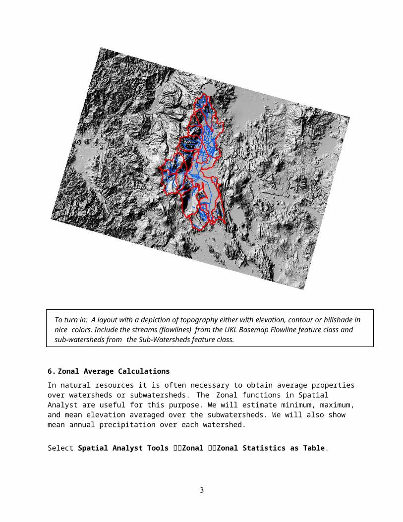
Click OK. You should see an illuminated hillshaded view of the topography. In our screen, we have turned on the flow line feature and the Subwatersheds feature and we have edited the symbology to make them show up well.

24

25

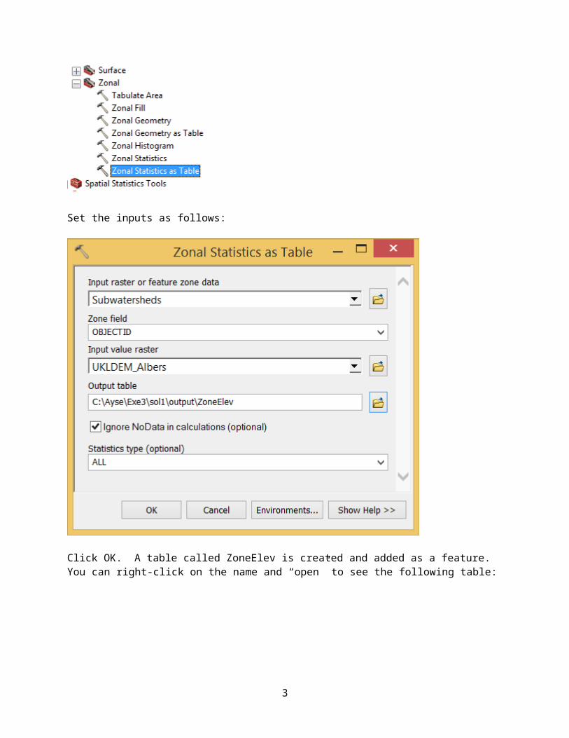
6. Zonal Average CalculationsIn natural resources it is often necessary to obtain average properties over watersheds or subwatersheds. The Zonal functions in Spatial Analyst are useful for this purpose. We will estimate minimum, maximum, and mean elevation averaged over the subwatersheds. We will also show mean annual precipitation over each watershed.

Select Spatial Analyst Tools Zonal Zonal Statistics as Table.

To turn in: A layout with a depiction of topography either with elevation, contour or hillshade in nice colors. Include the streams (flowlines) from the UKL Basemap Flowline feature class and sub-watersheds from the Sub-Watersheds feature class.

26

Set the inputs as follows:

Click OK. A table called ZoneElev is created and added as a feature. You can right-click on the name and “open” to see the following table:

27

This table contains statistics of the value raster, in this case elevation from ukldem_albers over the zones defined by the polygon feature class Subwatershed. Remember that there are 18 subwatersheds identified in the Subwatershed feature.

The Value field in this zone table contains the ObjectID from the subwatershed layer and may be used to join these values with attributes of the Subwatershed feature class.

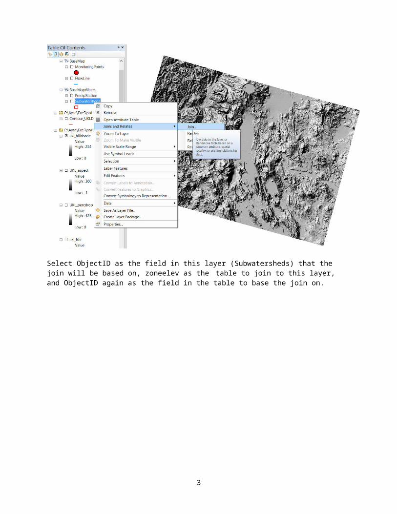
Right click on Subwatersheds and select Joins and Relates Join.

Question: what units are the “Area” values in? What units are the “Min” and “Max” units in?

28

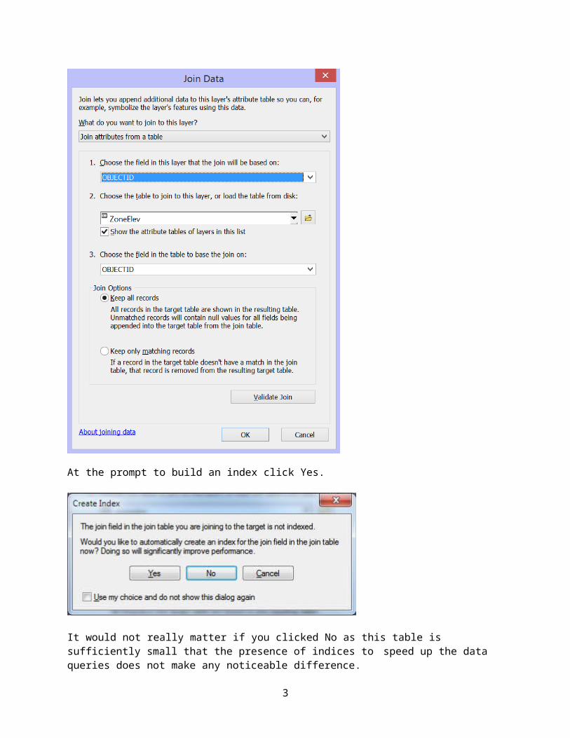
Select ObjectID as the field in this layer (Subwatersheds) that the join will be based on, zoneelev as the table to join to this layer, and ObjectID again as the field in the table to base the join on.

29

At the prompt to build an index click Yes.

It would not really matter if you clicked No as this table is sufficiently small that the presence of indices to speed up the data queries does not make any noticeable difference.

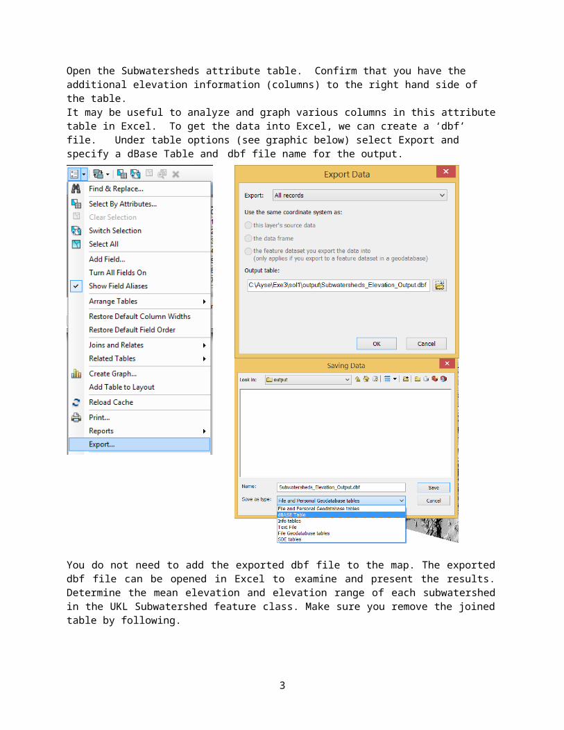
Open the Subwatersheds attribute table. Confirm that you have the additional elevation information (columns) to the right hand side of the table.

30

It may be useful to analyze and graph various columns in this attribute table in Excel. To get the data into Excel, we can create a ‘dbf’ file. Under table options (see graphic below) select Export and specify a dBase Table and dbf file name for the output.

You do not need to add the exported dbf file to the map. The exported dbf file can be opened in Excel to examine and present the results. Determine the mean elevation and elevation range of each subwatershed in the UKL Subwatershed feature class. Make sure you remove the joined table by following.

31

To turn in: A table giving the ObjectID, Name, mean elevation, and elevation range for each subwatershed in the UKL Subwatershed feature class. Which subwatershed has the highest mean elevation? Which subwatershed has the largest elevation range?

32

7. Calculation of Area Average Precipitation using Thiessen PolygonsNow we will make some calculations that are really useful in hydrologic studies. We will calculate the area average mean annual precipitation over the watershed using Thiessen polygons. Thiessen polygons associate each point in a watershed with the nearest rain gages.

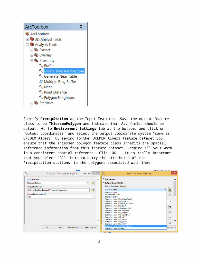
Select the tool Analysis Tools Proximity Create Thiessen Polygons

Specify PrecipStation as the Input Features. Save the output feature class to be ThiessenPolygon and indicate that ALL fields should be output. Go to Environment Settings tab at the bottom, and click on “Output coordinates” and select the output coordinate system “same as UKLDEM_Albers. By saving to

33

the UKLDEM_Albers feature dataset you ensure that the Thiessen polygon feature class inherits the spatial reference information from this feature dataset, keeping all your work in a consistent spatial reference. Click OK. It is really important that you select “All” here to carry the attributes of the Precipitation stations to the polygons associated with them.

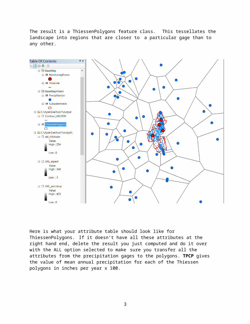
The result is a ThiessenPolygons feature class. This tessellates the landscape into regions that are closer to a particular gage than to any other.

34

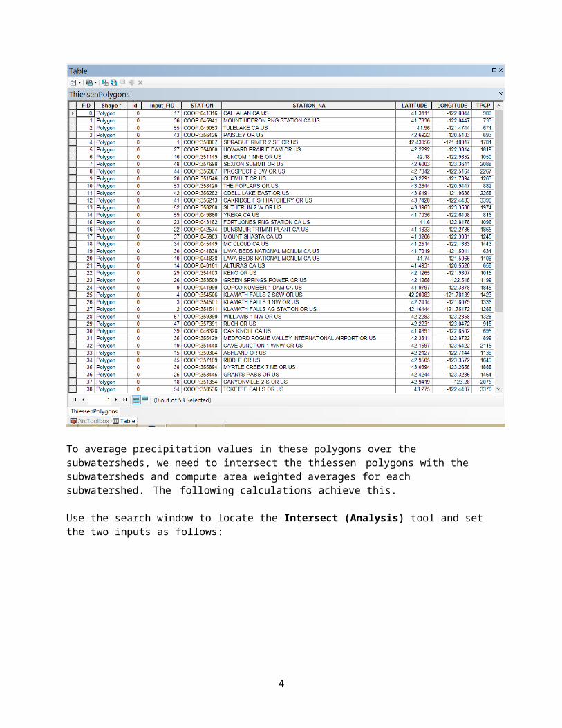
Here is what your attribute table should look like for ThiessenPolygons. If it doesn’t have all these attributes at the right hand end, delete the result you just computed and do it over with the ALL option selected to make sure you transfer all the attributes from the precipitation gages to the polygons. TPCP gives the value of mean annual precipitation for each of the Thiessen polygons in inches per year x 100.

35

To average precipitation values in these polygons over the subwatersheds, we need to intersect the thiessen polygons with the subwatersheds and compute area weighted averages for each subwatershed. The following calculations achieve this.

Use the search window to locate the Intersect (Analysis) tool and set the two inputs as follows:

36

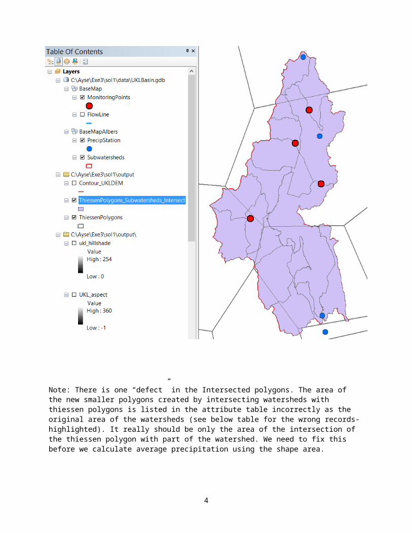
Following is the result:

37

Note: There is one “defect” in the Intersected polygons. The area of the new smaller polygons created by intersecting watersheds with thiessen polygons is listed in the attribute table incorrectly as the original area of the watersheds (see below table for the wrong records- highlighted). It really should be only the area of the intersection of the thiessen polygon with part of the watershed. We need to fix this before we calculate average precipitation using the shape area.

38

We will create a new attribute (column) in the attribute table for the Thiessen Polygons_subwatersheds_intersect layer. Inside attribute table, select “Add field” from table options icon in the upper left part of the table.

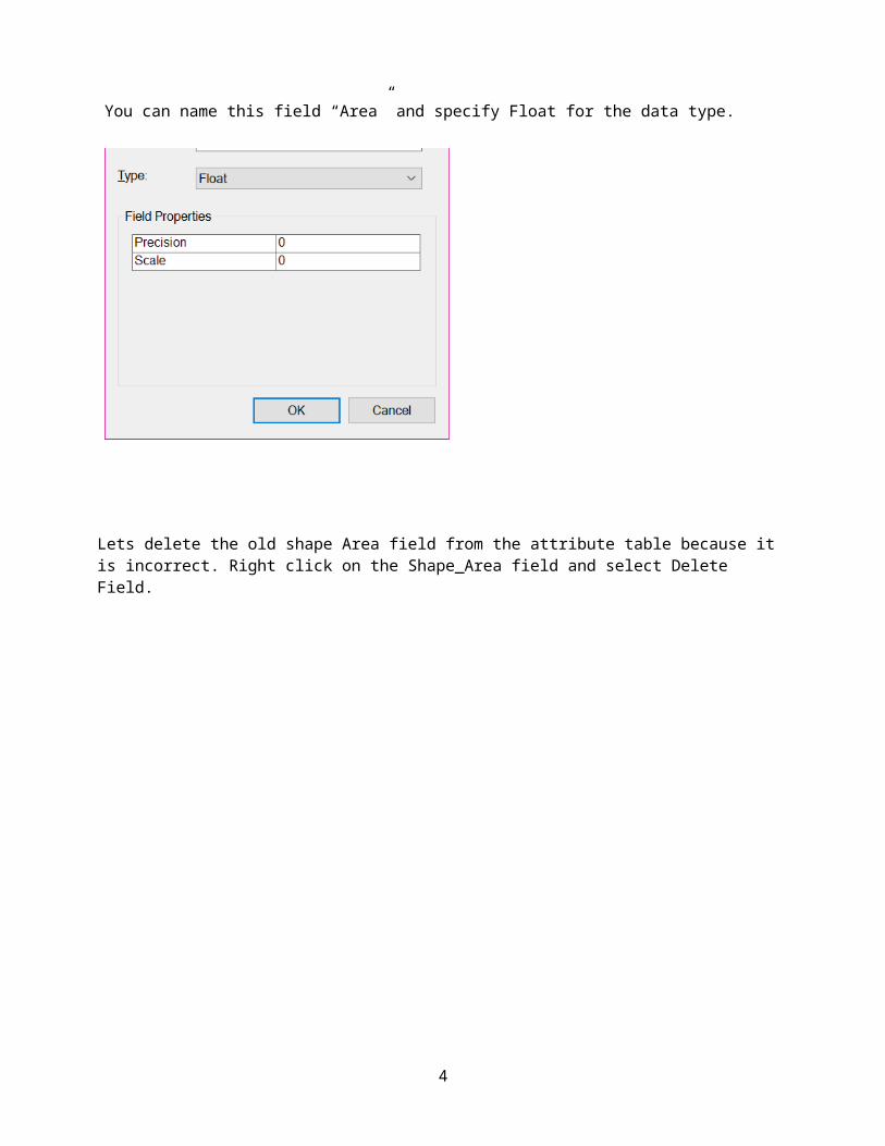
You can name this field “Area” and specify Float for the data type.

39

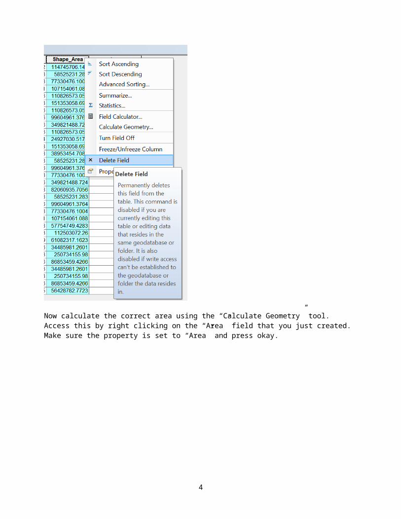
Lets delete the old shape Area field from the attribute table because it is incorrect. Right click on the Shape_Area field and select Delete Field.

40

Now calculate the correct area using the “Calculate Geometry” tool. Access this by right clicking on the “Area” field that you just created. Make sure the property is set to “Area” and press okay.

41

Now the areas shown represent the smaller shapes that were formed by intersecting thiessen polygons with subwatersheds.

The resulting table should look like the one below. I have turned off the attributes that I don’t want to see by going to layer properties by right clicking on the layer name and unchecking the fields I don’t want to see.

42

43

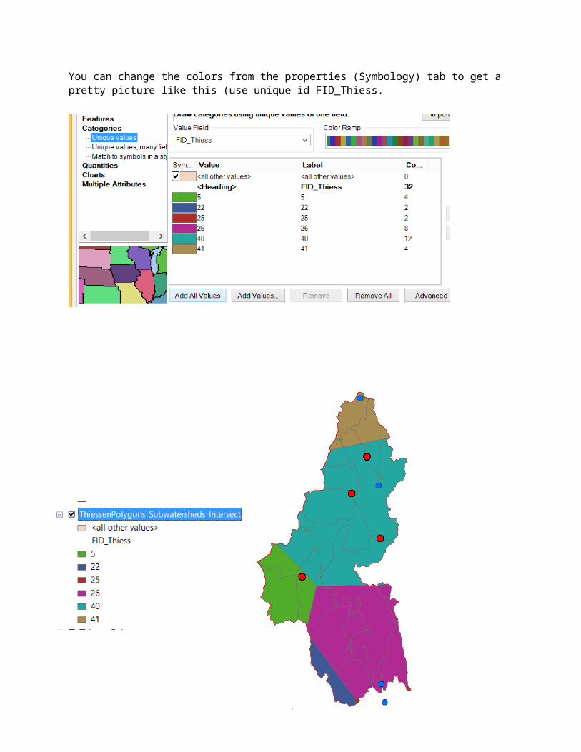
You can change the colors from the properties (Symbology) tab to get a pretty picture like this (use unique id FID_Thiess.

44

If you open the ThiessenSubwatershedsIntersect attribute table, you will see that from the 18 subwatersheds, there are now 32 polygons, each contributing to part of a subwatershed and associated with a single rain gage.

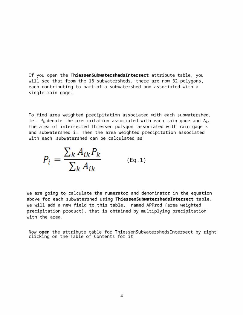
To find area weighted precipitation associated with each subwatershed, let Pk denote the precipitation associated with each rain gage and Aik the area of intersected Thiessen polygon associated with rain gage k and subwatershed i. Then the area weighted precipitation associated with each subwatershed can be calculated as

We are going to calculate the numerator and denominator in the equation above for each subwatershed using ThiessenSubwatershedsIntersect table. We will add a new field to this table, named APProd (area weighted precipitation product), that is obtained by multiplying precipitation with the area.

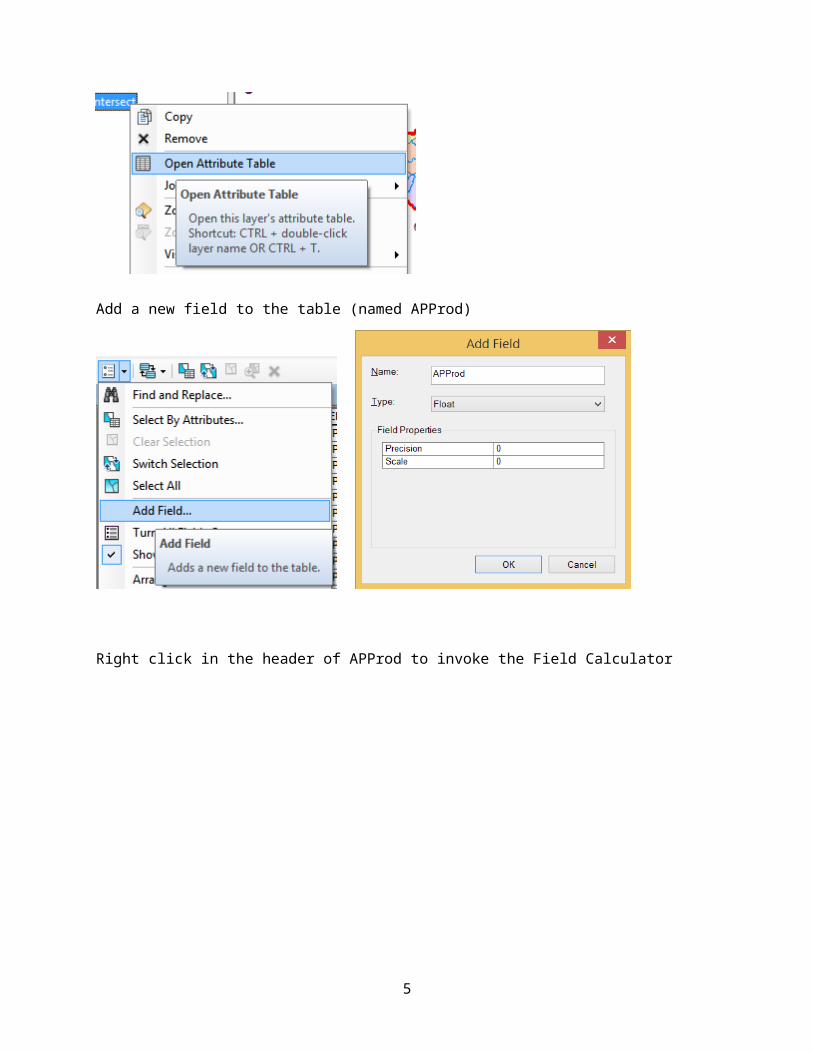
Now open the attribute table for ThiessenSubwatershedsIntersect by right clicking on the Table of Contents for it

Add a new field to the table (named APProd)

(Eq.1)

45

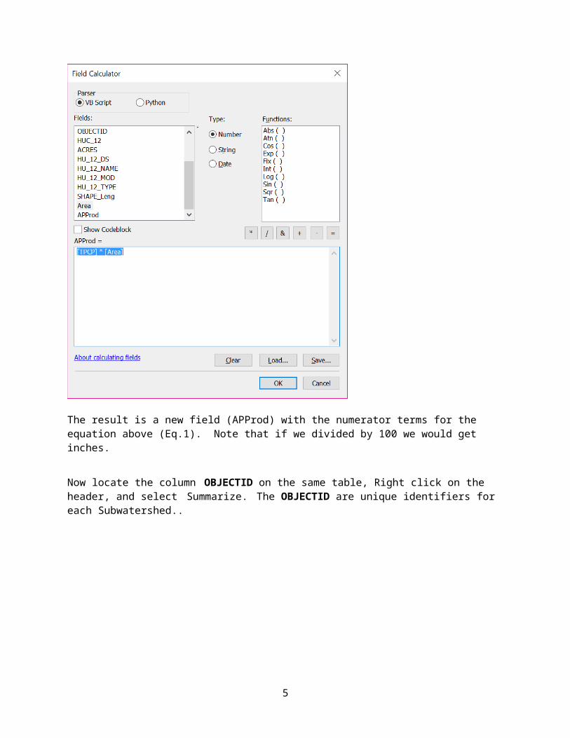
Right click in the header of APProd to invoke the Field Calculator

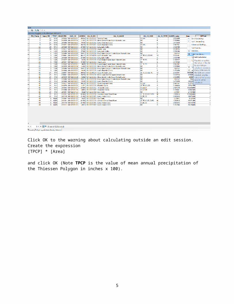
Click OK to the warning about calculating outside an edit session. Create the expression[TPCP] * [Area]

and click OK (Note TPCP is the value of mean annual precipitation of the Thiessen Polygon in inches x 100).

46

The result is a new field (APProd) with the numerator terms for the equation above (Eq.1). Note that if we divided by 100 we would get inches.

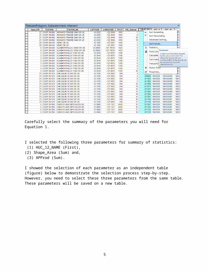
Now locate the column OBJECTID on the same table, Right click on the header, and select Summarize. The OBJECTID are unique identifiers for each Subwatershed..

47

Carefully select the summary of the parameters you will need for Equation 1.

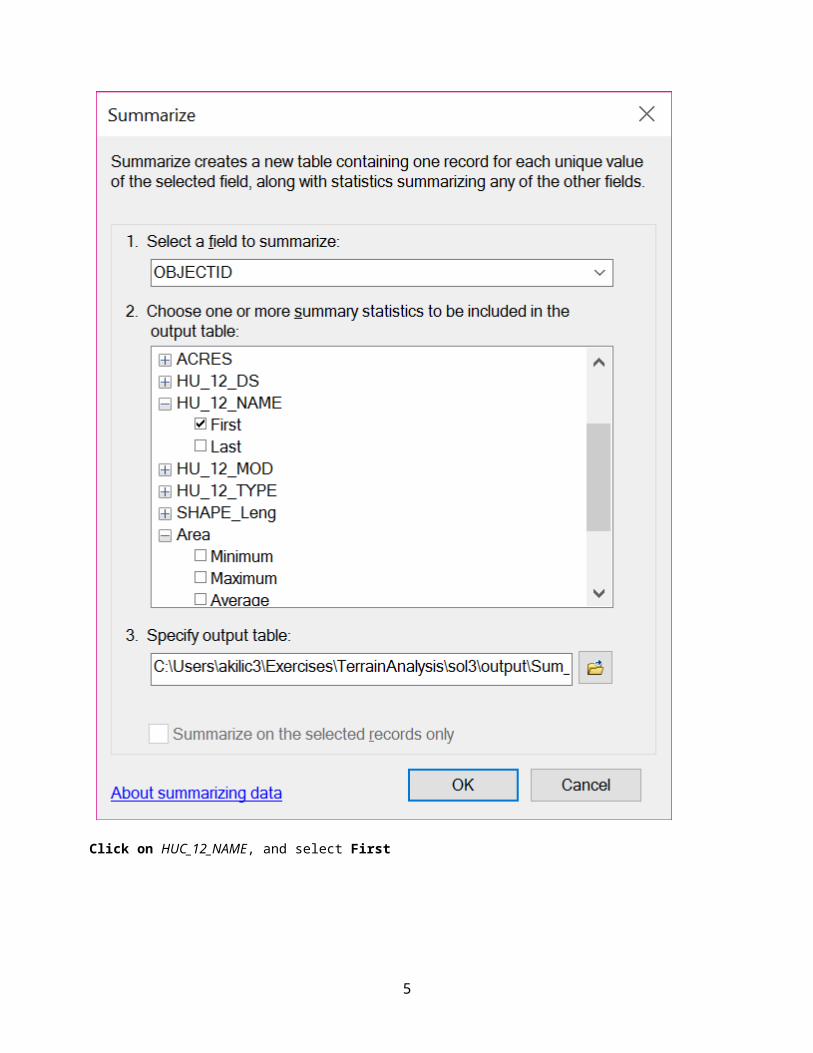
I selected the following three parameters for summary of statistics: (1) HUC_12_NAME (First), (2) Shape_Area (Sum) and, (3) APProd (Sum).

I showed the selection of each parameter as an independent table (figure) below to demonstrate the selection process step-by-step. However, you need to select these three parameters from the same table. These parameters will be saved on a new table.

48

Click on HUC_12_NAME, and select First

49

On the same table, Click on Shape Area, and check the Sum

On the same table, click on APProd and select Sum

50

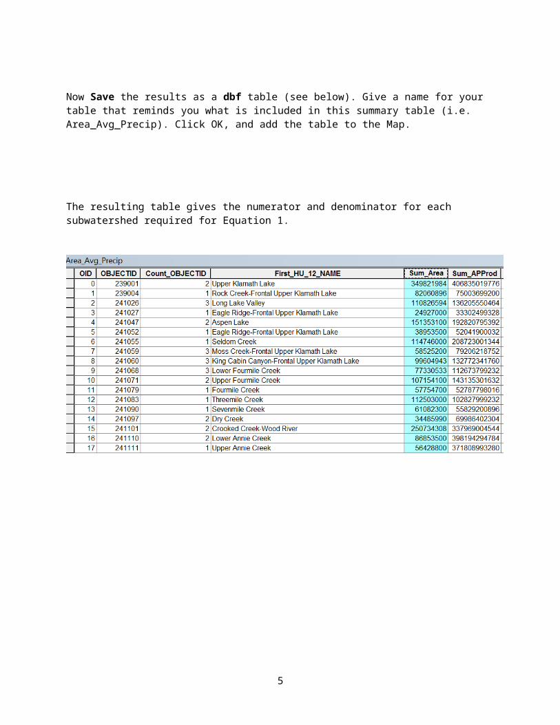
Now Save the results as a dbf table (see below). Give a name for your table that reminds you what is included in this summary table (i.e. Area_Avg_Precip). Click OK, and add the table to the Map.

The resulting table gives the numerator and denominator for each subwatershed required for Equation 1.

51

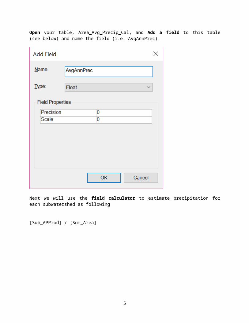
Open your table, Area_Avg_Precip_Cal, and Add a field to this table (see below) and name the field (i.e. AvgAnnPrec).

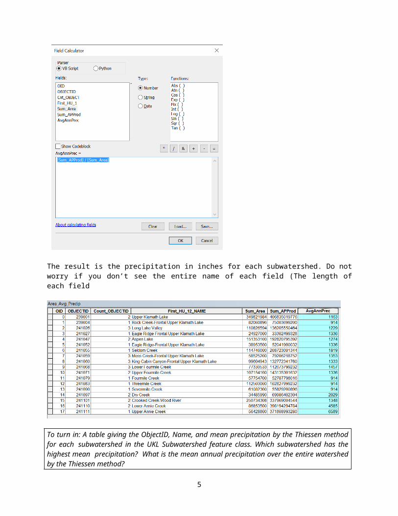
Next we will use the field calculator to estimate precipitation for each subwatershed as following

[Sum_APProd] / [Sum_Area]

52

The result is the precipitation in inches for each subwatershed. Do not worry if you don’t see the entire name of each field (The length of each field

To turn in: A table giving the ObjectID, Name, and mean precipitation by the Thiessen method for each subwatershed in the UKL Subwatershed feature class. Which subwatershed has the highest mean precipitation? What is the mean annual precipitation over the entire watershed by the Thiessen method?

53

8. Estimate basin average mean annual precipitation using Spatial Interpolation/Surface fitting.Thiessen polygons were effectively a way of defining a field based on discrete data, by associating with each point the precipitation at the nearest gage. This is probably the simplest and least sophisticated form of spatial interpolation. ArcGIS provides other spatial interpolation capabilities in the Interpolation toolbox in Spatial Analyst Tools.

We will not, in this exercise, concern ourselves too much with the theory behind each of these methods. You should however be aware that there is a lot of statistical theory on the subject of interpolation, which is an active area of research. This theory should be considered before practical use of these methods.

Select Spatial Analyst Tools Interpolation Spline. Use the input points from "PrecipStation" and Z value field as "TPCP", and set the spline type as Regularized with parameters as follows:

54

The result is as follows:

However, note that the ‘red’ and ‘orange’ areas are actually negative precipitation (as much as -43 inches!) (remember that TPCP is in inches x 100). Therefore, let’s use a spline with ‘tension’ instead. The tension will keep the peaks and valleys from getting too far beyond the measured data.

Select Spatial Analyst Tools Interpolation Spline. Use the input points from "PrecipStation" and Z value field as "TPCP", and set the spline type as Tension with parameters as follows. The default weighting for the tension is 0.1:

55

The result is illustrated:

56

The results are better, but still there is a small amount of negative (red color) area with a low of -1.8 inches. Let’s rerun one more time with a tension weight of 10:

57

Now the minimum value in the surface is 1.44 inches. One can experiment with different weights. Clearly, the ‘normal’ (regularized) spline should not be trusted, without review, for precipitation data.

Note how much more ‘realistic’ and continuous the splined surface is as compared to the Thiessen surface. The Thiessen surface is a series of ‘stair steps’ or ‘terraces’. There is no need to use the Thiessen with ArcMAP.

58

Statistics on the precipitation surfaceWe can produce statistics on the precipitation raster that we have created.Select Spatial Analyst Tools Zonal Zonal Statistics as Table. Set the inputs as follows:

59

Click OK. A table with zonal statistics is created. This contains statistics of the value raster, in this case mean annual precipitation from Spline over the zones defined by the polygon feature class Subwatershed. The ObjectID in this table may be used to join it to the attribute table for the Subwatershed feature class.

As for the elevations above this joined table can be exported and examined and presented in Excel.

To turn in: A table giving the ObjectID, Name, and mean precipitation by the Tension Spline method for each subwatershed in the UKL Subwatershed feature class.

Which subwatershed has the highest mean precipitation using a Tension Spline interpolation?

What is the mean annual precipitation over the entire watershed by the tension-spline method?

Experiment with some (at least one) of the other methods available (Natural Neighbor, Kriging, Inverse distance weighting) to see if you think that they are more accurate.To turn in. A layout giving a nicely colored map of the interpolated mean annual precipitation surface over the UKL Basin for one of the methods used and a table showing the mean annual precipitation for the same method in each Subwatershed. Report what method you used.

Summary of Items to turn in:

1. A table showing the number of columns and rows, cell size in the E-W and N-S directions in m, extent (in degrees) and spatial reference information for the UKL elevation dataset, 'rawdem'.

2. The number of columns and rows in the projected DEM. The minimum and maximum elevations in the projected DEM. Explain why the minimum and maximum elevations are different from the minimum and maximum elevations in the original DEM.3. A layout showing the location of the highest elevation value in the UKL DEM. Include a scale bar and north arrow in the layout.

4. A layout with a depiction of topography either with elevation, contour or hillshade in nice colors. Include the streams from the UKL Basemap Flowline feature class and sub-watersheds from the Sub-Watersheds feature class.

60

5. A table giving the ObjectID, Name, mean elevation, and elevation range for each subwatershed in the UKL Subwatershed feature class. Which subwatershed has the highest mean elevation? Which subwatershed has the largest elevation range?

6. A table giving the ObjectID, Name, and mean precipitation by the Thiessen method for each subwatershed in the UKL Subwatershed feature class. Which subwatershed has the highest mean precipitation? What is the mean annual precipitation over the entire watershed by the Thiessen method?

7. To turn in: A table giving the ObjectID, Name, and mean precipitation by the Tension Spline method for each subwatershed in the UKL Subwatershed feature class. Which subwatershed has the highest mean precipitation using a Tension Spline interpolation? What is the mean annual precipitation over the entire watershed by the tension-spline method?

8. A layout giving a nicely colored map of the interpolated mean annual precipitation surface over the UKL Basin for one of the methods used and a table showing the mean annual precipitation for the same method in each Subwatershed. Report what method you used.

Runoff Coefficients (Optional)

Runoff ratio, defined as the fraction of precipitation that becomes streamflow at a subbasin outlet is a useful measure in quantifying the hydrology of a watershed. Mathematically runoff ratio is defined as

w = Q/P

where Q is streamflow, and P is precipitation. In this formula, P and Q need to be in consistent units such as depth per unit area or volume. The flow field in the Monitoring point feature class gives the average streamflow at four monitoring points in the Klamath watershed in ft3/s. To convert these to volume units (say ft3) they should be multiplied by the number of seconds in a year (60 x 60 x 24 x 365.25). In the current exercise mean annual precipitation has been evaluated for each subwatershed, in inches. To convert these to volume units (say ft3) these quantities should be multiplied by 1/12 ft in-1

and multiplied by the subwatershed area in ft2. The subwatershed feature class includes subwatershed area, in the units of the spatial reference frame being used, which are m2. (Remember, 1 ft = 0.3048 m). The necessary calculations are most easily performed in Excel. Use the Options/Export function to export the subwatershed featureclass attribute table that includes your Thiessen basin average subwatershed precipitation results to dbf format that can be read by Excel, as was done above. Similarly export the Monitoring Point featureclass attribute table that includes mean annual streamflow at each monitoring point. In Excel multiply gage streamflow by 60 x 60 x 24 x 365.25 to obtain streamflow volume, Q, in ft3. Multiply subwatershed average precipitation (in inches) by subwatershed area (in m2)/(12 x 0.30482) to obtain subwatershed precipitation volume, P, in ft3. On the maps you have that show subwatersheds and streams identify the subwatersheds upstream of each gauge. Do this visually by looking at the Flowlines. Add up the precipitation volumes over these subwatersheds then divide Q/P to obtain an estimate of runoff ratio for the watershed upstream of each stream gage.

To turn in. A table giving runoff ratio for the watershed upstream of each stream gage.