Examining the advantages and disadvantages of pilot ...

University of New MexicoUNM Digital Repository

Psychology ETDs Electronic Theses and Dissertations

2-1-2012

Examining the advantages and disadvantages ofpilot studies : Monte-Carlo simulationsMasato Nakazawa

Follow this and additional works at: https://digitalrepository.unm.edu/psy_etds

This Dissertation is brought to you for free and open access by the Electronic Theses and Dissertations at UNM Digital Repository. It has beenaccepted for inclusion in Psychology ETDs by an authorized administrator of UNM Digital Repository. For more information, please [email protected].

Recommended CitationNakazawa, Masato. "Examining the advantages and disadvantages of pilot studies : Monte-Carlo simulations." (2012).https://digitalrepository.unm.edu/psy_etds/104

https://digitalrepository.unm.edu?utm_source=digitalrepository.unm.edu%2Fpsy_etds%2F104&utm_medium=PDF&utm_campaign=PDFCoverPages

https://digitalrepository.unm.edu/psy_etds?utm_source=digitalrepository.unm.edu%2Fpsy_etds%2F104&utm_medium=PDF&utm_campaign=PDFCoverPages

https://digitalrepository.unm.edu/etds?utm_source=digitalrepository.unm.edu%2Fpsy_etds%2F104&utm_medium=PDF&utm_campaign=PDFCoverPages

https://digitalrepository.unm.edu/psy_etds?utm_source=digitalrepository.unm.edu%2Fpsy_etds%2F104&utm_medium=PDF&utm_campaign=PDFCoverPages

https://digitalrepository.unm.edu/psy_etds/104?utm_source=digitalrepository.unm.edu%2Fpsy_etds%2F104&utm_medium=PDF&utm_campaign=PDFCoverPages

mailto:[email protected]

Examining the Advantages and Disadvantages of Pilot Studies: Monte-

Carlo Simulations

BY

Masato Nakazawa

B.S., History, the University of California, Los Angeles, 2000

M.A., Psychology, the University of New Mexico, 2006

DISSERTATION

Submitted in Partial Fulfillment of the

Requirements for the Degree of

Doctor of Philosophy

Psychology

The University of New Mexico

Albuquerque, New Mexico

December, 2011

iii

©2011, Masato Nakazawa

iv

ACKNOWLEDGMENTS

I heartily acknowledge Dr. Harold Delaney, my advisor and dissertation chair, for

continuing to encourage me through the years of classroom teachings and for his infinite

patience in reading my manuscript and giving me feedback. His guidance and

professionalism will remain with me as I continue my career.

I also thank my committee members, Dr. Angela Bryan, Dr. Timothy Goldsmith,

and Dr. Jay Parkes, for their valuable suggestions and encouragement that played an

important role in shaping this study and my professional development.

And finally to my wife, Yea-Wen Chen. You bestowed the greatest gifts of love

and encouragement upon me. This dissertation is our accomplishment.

Examining the Advantages and Disadvantages of Pilot Studies: Monte-

Carlo Simulations

BY

Masato Nakazawa

ABSTRACT OF DISSERTATION

Submitted in Partial Fulfillment of the

Requirements for the Degree of

Doctor of Philosophy

Psychology

The University of New Mexico

Albuquerque, New Mexico

December, 2011

vi

Examining the Advantages and Disadvantages of Pilot Studies: Monte-Carlo

Simulations

By

Masato Nakazawa

B.A. in History, University of California, Los Angeles, 2000

M.S. in Psychology, University of New Mexico, 2006

Ph.D. in Psychology, University of New Mexico, 2011

Abstract

Estimating population effect size accurately and precisely plays a vital role in

achieving a desired level of statistical power as well as drawing correct conclusions from

empirical results. While a number of common practices of effect-size estimation have

been documented (e.g., relying on one’s experience and intuition, and conducting pilot

studies), their relative advantages and disadvantages have been insufficiently

investigated. To establish a practical guideline for researchers in this respect, this project

compared the accuracy and precision of effect-size estimation, resulting power, and

economic implications across pilot and non-pilot conditions. Furthermore, to model the

potential advantages of conducting pilot studies in finding and correcting flaws before

main studies are run, varying amounts of random error variance and varying degrees of

vii

success at its removal – often neglected aspects in simulation studies – were introduced in

Experiment 2.

The main findings include the following. First, pilot studies with up to 30 subjects

were utterly ineffective in achieving the desired power of 0.80 at a small population

effect size even under the best-case scenario. At this effect size, intuitive estimation

without pilot studies appears to be the preferred method of achieving the desired power.

Second, the pilot studies performed better at medium and large population effect sizes,

achieving comparable or even greater power to that in the non-pilot condition. The

relative advantages of pilot studies were particularly evident when moderate to large error

variances were present, and a portion of it had been removed through conducting pilot

studies. These broad findings are discussed in the context of flexible design: study design

can be modified flexibly in accordance with the researcher’s particular goals.

viii

TABLE OF CONTENTS

LIST OF FIGURES………………………………………………………………...… …xii

LIST OF TABLES……………………………………………………………………... xiii

CHAPTER 1 INTRODUCTION…………………………………………………….…… 1

Importance of Power…………………………………………………………………. 1

Practices of Effect-Size Estimation………………………………………………...… 5

CHAPTER 2 OBJECTIVES OF THE CURRENT STUDY……………………………. 11

Objective 1…………………………………………………………………………... 11

Objective 2…………………………………………………………………………... 11

Objective 3…………………………………………………………………………... 12

CHAPTER 3 GENERAL METHOD…………………………………………………….15

Procedure……………………………………………………………………………. 15

Independent Variables………………………………………………………………. 17

Dependent Variables………………………………………………………………... 18

Estimated required sample size………………………………………………….18

Power deviation………………………………………………………………….18

Measures of accuracy and precision of effect-size estimation…………………..19

Measures of economic performance…………………………………………….20

Cost per percentage point………………………………………………… 20

Expected wasted resources…………………………………………………21

CHAPTER 4 EXPERIMENT 1………………………………………………………… 23

Method……………………………………………………………………………… 23

Effect-size Estimation methods………………………………………………….23

Hedges formula………………………………………………………………25

ix

Wherry formula……………………………………………………………. 25

Maxwell-Delaney (MD) formula…………………………………………... 25

Upper one-sided confidence limit (UCL)………………………………….. 26

Results……………………………………………………………………………….. 27

Observed effect sizes …………………………………………………27

Measures of accuracy of effect-size estimation…………………………... ..27

Overall impression……………………………………………………… .28

Cohen’s d………………………………………………………………... 28

Hedges formula………………………………………………………….. 31

Wherry formula…………………………………………………………. 31

Maxwell-Delaney (MD) formula………………………………………... 31

Upper one-sided confidence limit (UCL)……………………………….. 32

Measures of precision of effect-size estimation………………………..….. .32

Overall impression………………………………………………………. 32

Cohen’s d………………………………………………………………... 34

Hedges formula and UCL………………………………………………. 34

Wherry and MD formulae……………………………………………….. 35

Ninety-five percent confidence interval around observed effect size…………… 35

Estimated required sample size………………………………………………. ….38

Overall impression…………………………………………………………. 39

Cohen’s d…………………………………………………………………… 41

Hedges formula……………………………………………………………...41

Wherry and MD formulae…………………………………………………...42

UCL…………………………………………..……………………………...42

Probability of the main study being aborted…………………………………..…43

x

Power Deviation………………………………………………………………….43

Power deviation – total power……………………………………………….45

Power deviation – valid power………………………………………………48

Measures of economic performance……………………………………………..48

Power, EWR, and CCP of studies conducted without pilot studies……………...53

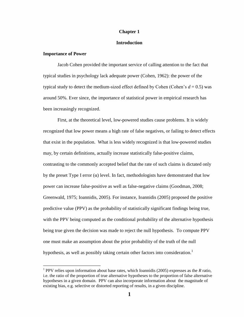
Null effect size…………………………………………………………………...58

Discussion……………………………………………………………………………59

CHAPTER 5 EXPERIMENT 2………………………………………………………….64

Method……………………………………………………………………………….64

Size of population error variance………………………………………………...67

Size of reduction in the error variance…………………………………………...69

Results………………………………………………………………………………..70

Observed effect sizes ……………………………………………………………70

Measures of accuracy of effect-size estimation……………………………...71

Error variance of 56%……………………………………………………71

Error variance of 125% and 300%……………………………………….72

Measures of precision of effect-size estimation……………………………...73

Estimated required sample size…………………………………………………..73

Probability of the main study being aborted……………………………………..75

Power Deviation………………………………………………………………….77

Power deviation – total power……………………………………………….77

Power deviation – valid power………………………………………………80

Measures of economic performance……………………………………………..80

Power, EWR, and CCP of studies conducted without pilot studies……………..83

Null effect size…………………………………………………………………...88

xi

Discussion……………………………………………………………………………89

CHAPTER 6 SUMMARY AND CONCLUDING DISCUSSION ……………………..92

Objective 1…………………………………………………………………………...92

Accuracy and precision in estimating population effect sizes…………………...92

Accuracy and precision in estimating required sample sizes and the resulting

power …………………………………………………………………..……92

Comparison with the non-pilot condition…………………..……………………93

Objective-1 conclusion…………………………………………………………..94

Objective 2…………………………………………………………………………..95

Objective-1 conclusion………………………………………………………….97

Objective 3…………………………………………………………………………..98

Accuracy and precision in estimating population effect sizes and required

sample sizes…………………………………………………………………99

Effects of the error variance and its removal on power…………………..…….99

Comparison with the non-pilot condition…………………..………………….100

Effects of the error variance and its removal on economic performance……..100

Objective-3 conclusion………………………………………………………...101

Limitations…………………………………………………………………………102

Concluding remarks………………………………………………………………..105

APPENDICES………………………………………………………………………….108

Appendix A Formulae for Computing the Variance of the Sampling Distribution

of Cohen’s d……………………………………………………………………109

Appendix B R Code Used to Carry Out Simulations for the Current Study……..111

REFERENCES…………………………………………………………………………115

xii

LIST OF TABLES

Table 4.1. Descriptive Statistics for Estimated Effect Size in Experiment 1……………27

Table 4.2. Descriptive Statistics for 95% Confidence Intervals around Observed Effect

Size in Experiment 1………………………………………………………………..36

Table 4.3. Quantiles of the Distribution of Estimated Required Sample Size in

Experiment 1………………………………………………………………………..40

Table 4.4. Measures of Economic Efficiency in Experiment 1……………………….…49

Table 4.5. Effects of Pilot Sample Size and Estimation Methods on Type-I Error Rates in

Experiment 1………………………………………………………………………..59

Table 5.1. Descriptive Statistics for Estimated Effect Size in Experiment 2 – No Error

Variance Removed …………………………………………………………………70

Table 5.2. Quantiles of the Distribution of Estimated Required Sample Size ( ) in

Experiment 2 – No Error Variance Removed………………………………………74

Table 5.3. Expected Wasted Resources in Experiment 2………………………….…….81

Table 5.4. Cost per Percentage Point in Experiment 2…………………………………..81

Table 5.5. Effects of Sample Size and δ on Power, Expected Wasted Resources, and Cost

per Percentage Point in Main Studies Conducted without Pilot Studies in Experiment

2……………………………………………………………………………………..87

Table 5.6. Effects of Pilot Sample Size, Error-Variance Size, and Proportion of Error

Variance Removed on Type-I Error Rates in Experiment 2 (10000

Replications)………………………………………………………………………..89

xiii

LIST OF FIGURES

Figure 4.1. Procedural Steps for Experiment-1 Pilot Condition…………………………24

Figure 4.2. Procedural Steps for Experiment-1 Non-Pilot Condition……………………24

Figure 4.3. Effects of Estimation Methods and Pilot Sample Size (NPilot) on the Mean

Observed Effect Size (d)……………………………………………………………29

Figure 4.4. Effects of Estimation Methods and Pilot Sample Size (NPilot) on the Median

Observed Effect Size (d)……………………………………………………………30

Figure 4.5. Effects of Estimation Methods and Pilot Sample Size (NPilot) on the

Distribution of Observed Effect Size (d) in Experiment 1………………………….33

Figure 4.6. Probability of the Main Study being Aborted Based on Pilot Results……....44

Figure 4.7. Power Deviation Derived from the Power Based on All Studies (Total Power

– 0.8)……………………………………………………………………………..46

Figure 4.8. Power Deviation Derived from the Power Based on Valid Studies (Valid

Power – 0.8)…………………………………………………………………………47

Figure 4.9. Wasted Resources ([Median Total Study Cost] * [1 – Total Power])……….51

Figure 4.10. Cost per Percentage Point ([Median Total Study Cost] / [Total Power *

100])………………………………………………………………………………...52

Figure 4.11. The Tolerance Range of Underestimated Population Effect Size for Studies

Conducted without Pilot Studies……………………………………………………55

Figure 4.12. Effects of Sample Size (N) and Population Effect Size (δ) on: (a) Power, (b)

Expected Wasted Resources (EWR), and (c) Cost per Percentage Point (CPP) in

Main Studies Conducted without Pilot Studies in Experiment 1…………………...57

xiv

Figure 4.13. Different proportions of the theoretical distribution of Cohen’s d…..……..61

Figure 5.1. Procedural Steps for Experiment 2 Pilot Condition…………………………65

Figure 5.2. Procedural Steps for Experiment 2 Non-Pilot Condition……………………66

Figure 5.3. Probability of the Main Study Being Aborted Based on Pilot Results in

Experiment 2………………………………………………………………………..76

Figure 5.4. Power Deviation Based on Total Power (Total Power – 0.8) in Experiment

2……………………………………………………………………………………..78

Figure 5.5. Power Deviation Based on Valid Power (Valid Power – 0.8) in Experiment

2……………………………………………………………………………………..78

1

Chapter 1

Introduction

Importance of Power

Jacob Cohen provided the important service of calling attention to the fact that

typical studies in psychology lack adequate power (Cohen, 1962): the power of the

typical study to detect the medium-sized effect defined by Cohen (Cohen’s d = 0.5) was

around 50%. Ever since, the importance of statistical power in empirical research has

been increasingly recognized.

First, at the theoretical level, low-powered studies cause problems. It is widely

recognized that low power means a high rate of false negatives, or failing to detect effects

that exist in the population. What is less widely recognized is that low-powered studies

may, by certain definitions, actually increase statistically false-positive claims,

contrasting to the commonly accepted belief that the rate of such claims is dictated only

by the preset Type I error (α) level. In fact, methodologists have demonstrated that low

power can increase false-positive as well as false-negative claims (Goodman, 2008;

Greenwald, 1975; Ioannidis, 2005). For instance, Ioannidis (2005) proposed the positive

predictive value (PPV) as the probability of statistically significant findings being true,

with the PPV being computed as the conditional probability of the alternative hypothesis

being true given the decision was made to reject the null hypothesis. To compute PPV

one must make an assumption about the prior probability of the truth of the null

hypothesis, as well as possibly taking certain other factors into consideration.1

1 PPV relies upon information about base rates, which Ioannidis (2005) expresses as the R ratio,

i.e. the ratio of the proportion of true alternative hypotheses to the proportion of false alternative

hypotheses in a given domain. PPV can also incorporate information about the magnitude of

existing bias, e.g. selective or distorted reporting of results, in a given discipline.

2

Conversely, negative predictive value (NPV) was defined as 1 – PPV, an index of the

false-positive error rate. Although NPV is somewhat similar to the Type I error rate, in

that the numerator reflects the number of true null hypotheses falsely rejected, the key

difference between these two indices is that NPV is the conditional probability of being

wrong given the null hypothesis was rejected, i.e. the denominator reflects the number of

rejected hypotheses, not the number of true null hypotheses tested as in the computation

of Type I error rates. Low power, with everything else being equal, also increases NPV:

lowering power from 0.8 to 0.5 (which lowers the number of false null hypotheses that

are correctly rejected) increased NPV by 0.03~0.05. Thus, low power increases not only

the false-negative error rates (i.e., the Type II error rate, β) but also could potentially

increase false-positive error rates (i.e., NPV), thereby limiting the value of the results

from low-powered studies. This problem of low power poses a serious challenge to

researchers, who are mainly concerned with discovering causal relationships and

explaining natural phenomena (Shadish, Cook, & Campbell, 2001): increased error rates

can compromise the validity of their findings.

Furthermore, the practice of conducting low-powered (LP) studies has been

criticized by various methodologists because such studies potentially waste valuable

resources and mislead participants (Breau, Carnat, & Gaboury, 2006; Legg & Nagy,

2006; Turner, Matthews, Linardatos, Tell, & Rosenthal, 2008). To demonstrate this

numerically, consider a research scenario where the base cost of conducting a particular

experiment is $5,000, and recruiting subjects costs $100 each. Also suppose that

researcher A, trying to reduce the overall cost of the study, recruits only 60 subjects; thus,

the total cost of his experiment is $5,000 + 60 x $100 = $11,000. On the other hand,

3

researcher B, being power conscious, recruits 170 subjects to achieve sufficient power,

costing the total of $22,000. Assuming the typical α level of 0.05 and population effect

size (standardized mean difference) of 0.5, the power of experiment A is merely 0.49

whereas that of experiment B is 0.90. If both researchers A and B were to repeat the

experiments under the same configurations, more than 50% (1 – 0.49 = 0.51) of

replicated experiments A would yield statistically non-significant results, whereas that is

true in only 10% of replicated experiments B. Now let us assume that all of the

significant results are “used, published” but all of the non-significant results are

“wasted.” Then, for each experiment A conducted, (1 - 0.4906) x $11,000 = $5,603

would be wasted in the long run, whereas the comparable figure for B would only be (1 -

.9) x $22,000 = $2,200. Taking this argument to the extreme, a few methodologists even

call low powered, potentially wasteful studies unethical (Halpern, Karlawish, & Berlin,

2002).

At the practical level, high statistical power is more desirable because low-

powered studies tend to produce non-significant results. Because non-significant results

are hard to publish, conducting a series of LP studies can impact negatively the

researcher’s career (Hojat, Gonnella, & Caelleigh, 2003). At the same time, researchers’

primary sources of funding, i.e., granting agencies, increasingly require sufficient

statistical power before funding large scale studies (Lilford, Thornton, & Braunholtz,

1995; Sherrill et al., 2009). Designing low-powered studies may prevent researchers from

obtaining funding, further compromising their productivity. Thus, from both theoretical

and practical perspectives, achieving desired power plays a vital role in empirical

research.

4

A crucial step in achieving desired power is accurate sample size calculation,

which involves three components: α (the Type I error rate), a desired level of power (1 –

β, where β is the Type II error rate), and estimated population effect size (Kraemer,

1991). Of these components, α and desired power are typically fixed by convention (Legg

& Nagy, 2006). Therefore, required sample size is determined by estimated population

effect size whose true value is rarely known in the social sciences. This statement has an

important implication: how accurately one estimates the population effect size of his/her

interest can dramatically influence the estimated required sample size, which in turn

affects the resulting power of the main study greatly (Browne, 2001; Johnston, Hays, &

Hui, 2009; Julious & Owen, 2006).

How an inaccurate and imprecise estimation of population effect size could

invalidate the conclusion of one’s study is illustrated here. If the estimation were

imprecise, for instance, researchers could estimate a null population effect size as small

to medium and conduct a study in pursuit of a treatment effect that does not truly exist

(Kraemer, Gardner, Brooks, & Yesavage, 1998). Conversely, researchers may

misestimate medium to large population effect sizes as close to null; as a result, they may

be discouraged by the inappropriately small estimated effect size and abandon the study

altogether (Kraemer, Mintz, Noda, Tinklenberg, & Yesavage, 2006).

Imprecise estimation processes can result in effect sizes that are overestimated

(i.e., estimated effect size is greater than its population counterpart) or underestimated

(i.e., estimated effect size smaller). Overestimation results in a calculated sample size

smaller than the true sample size needed to achieve the desired level of power. As a

result, the actual power of the study is lower than the desired power (underpowered

5

studies). If the effect size is underestimated, the calculated sample size will be larger than

true sample size required, resulting in overpowered studies. Overpowered studies may

appear advantageous compared to underpowered studies since they achieve higher-than-

desired power. But such studies may waste resources for a small increase in power,

especially when the effect size is small (e.g., in a two-group study, given a population

effect size of 0.2, increasing power from 0.85 to 0.90 requires 152 additional participants,

because the required total sample size increases from 902 to 1054). Thus, inaccurately

and/or imprecisely estimating effect size potentially has serious repercussions for the

study and its outcomes.

Practices of Effect-Size Estimation

Despite the vital importance of accuracy and precision in estimating effect-size

while designing a study, there is no consensus regarding how it should best be estimated,

and researchers are often left wondering which of the several commonly used approaches

would be the most appropriate. To illustrate how pervasive this lack of guidance is it may

be noted that even the Consolidated Standards of Reporting Trials statement, requiring

researchers to report how they estimated the population effect size and calculated the

required sample size (Altman et al., 2001; Begg et al., 1996; Moher et al., 2010), does not

inform researchers about what may be the best practice of estimation. In the following

section, a number of common practices of effect-size estimation will be reviewed.

First, researchers may choose values based on their experience and intuition.

Assume that researchers are attempting to estimate population effect sizes for

experimental studies consisting of multiple groups. They initially define a likely

outcome, typically in a form of a difference in means between two or more groups. They

6

subsequently estimate the population parameter of variability (e.g., the standard

deviation) associated with the outcome and divide the mean difference by the standard

deviation to derive a standardized mean difference (Altman, Moher, & Schulz, 2002;

Lenth, 2001, 2007; Schulz & Grimes, 2005). Based on this value of estimated effect size,

a necessary sample size to achieve a desired power (typically 0.80) is calculated.

Researchers may skip directly to estimating the standardized mean difference of interest

if a unit of measurement does not have a particularly well defined meaning. For instance,

while a number of standard drinks consumed per week or a number of cigarettes smoked

per day is based on a well defined, meaningful unit of measurement, the total score of the

Beck Depression Inventory or the score of a pain scale is not.

One obvious advantage of using one’s intuition and experience is that those may

be the only available source of estimation especially if there are no published studies

similar to a planned study. The estimation method based on one’s intuition may further

be enhanced by supplementing and restraining the range of estimation by the commonly

found effect size in a particular discipline (e.g., 0.5 in social sciences, Lipsey & Wilson,

1993) or criteria such as a minimally important difference2 (Harris & Quade, 1992;

Scales & Rubenfeld, 2005).

Second, researchers may consult published results from studies similar to their

own (Kraemer et al., 2006). The assumption here is that, if the targeted constructs and

research procedures employed in the published studies are similar enough to theirs, the

estimated population effect size reported in the studies should be used as the estimate of

2 Harris and Quade (1992) suggested the use of minimally important difference as a criterion for

sample size with which researchers would achieve power of 0.50. They argued that if the

population effect size were actually larger than the minimally important difference, the power

would be greater than 0.50; otherwise, it would be smaller than 0.50.

7

their own effect size. This value of the estimated effect is used as a guide to calculate a

necessary sample size to achieve a desired power. If an appropriate meta-analyses is

available, researchers can find a range of potential estimated effect sizes (Cohn &

Becker, 2003). One advantage of consulting published studies is that, because these

studies typically are well powered, the estimated population effect size reported tends to

be accurate (Kraemer et al., 2006), even though this is not always the case (Ioannidis,

2005; Ioannidis & Trikalinos, 2007; Kraemer et al., 1998).

Third, researchers may wish to conduct a small-scale pilot study (Browne, 1995;

Kraemer et al., 2006). The basic process of using a pilot study to estimate population

effect size is as follows. Initially researchers run a small-scale study following the same

study protocol as the main study. From the pilot study they obtain sample statistics such

as the mean and the standard deviation to estimate population parameters based on which

they compute estimated population effect sizes and calculate required sample size to

achieve the desired power level. 3

The size of the pilot studies is rarely discussed in the

literature, but one article recommends at least around 30 subjects for studies with two

independent groups (Hertzog, 2008). This sample size was used in at least one published

study (C. J. Wu, Chang, Courtney, Shortridge-Baggett, & Kostner, 2011a).

The advantages of conducting pilot studies over the other options have been well

documented. It allows researchers to estimate the effect size for their particular treatment.

3 This practice of conducting pilot studies is called external pilot studies because the pilot data are

assumed to be excluded from the final analysis. In contrast, if pilot data are incorporated into the

final analysis with appropriate α modifications, such study design is called internal pilot design

(Wittes & Brittain, 1990; Zucker, Wittes, Schabenberger, & Brittain, 1999) or adaptive design

(Brown et al., 2009). Though valid and potentially valuable, internal pilot design was not

included in the current project because this design assumes that the pilot and main studies share

the same protocol. This assumption is not held in the current project, especially in Experiment 2

where the main study is assumed to be deliberately modified, based on pilot results, to improve

study design.

8

This aspect of conducting pilot studies is particularly important if researchers cannot find

any published articles on studies similar to theirs. It also allows researchers to test

instruments and to assess the integrity of their study protocol. That is, before the actual

studies, researchers are able to find and eliminate any glitches using the results from the

pilot studies, making sure that the proposed studies are feasible as well as of high quality

(Arain, Campbell, Cooper, & Lancaster, 2010; Arnold et al., 2009; Hertzog, 2008;

Kraemer et al., 2006; Lancaster, Dodd, & Williamson, 2004; Thabane et al., 2010; S. S.

Wu & Yang, 2007).

On the other hand, conducting small-scale pilot studies to estimate effect size has

major disadvantages. First, its small sample size (N may be as small as 5, Arain et al.,

2010) can introduce bias in estimating effect size. For instance, Cohen’s d, an effect size

index for the popular independent-sample t test, is a positively biased estimator of its

population parameter, δ (Hedges & Olkin, 1985; Hunter & Schmidt, 2004). While this

bias is negligible with medium to large sample size (i.e., N > 50), its magnitude increases

as N decreases, reaching 11% with N = 8 (Hedges & Olkin, 1985, p. 84). Second,

Cohen’s d derived from small pilot studies tends to be imprecise in estimating δ (Hedges

& Olkin, 1985). In an two-group equal-n study, the variance of the sampling distribution

of Cohen’s d may be approximated as

(1)

(adapted from Hedges & Olkin, 1985, pp. 80, 104; see Appendix A ). According to this

formula, the standard deviation of Cohen’s d is larger than 0.73 at N = 10 and larger than

1.15 at N = 6 regardless of the size of δ. These are huge standard deviations considering

the mean effect size of 0.2~0.8! Because of these disadvantages – bias and imprecision

9

inherent in small-scale studies – some researchers caution against the use of pilot studies

in estimating effect size and hence calculating sample size (Kraemer et al, 1998, 2006).

Despite these disadvantages, the pilot-study approach is popular, especially in clinical

fields (Arain et al., 2010; Conn, Algase, Rawl, Zerwic, & Wyman, 2011; Hertzog, 2008;

Lancaster et al., 2004; C. J. Wu et al., 2011a).

As we have seen, conducting small-scale pilot studies is a biased and imprecise

method of estimating effect size. At the same time, the other methods mentioned above –

consulting appropriate meta-analyses and intuitively choosing values – can pose certain

challenges to researchers in accurately estimating population effect size. Even in

published studies, estimated population effect size can be biased especially if the studies

have small sample sizes and are low powered (Ioannidis, 2005, 2008), or if they employ

questionable statistical practices such as multiple testing without appropriate correction

(Maxwell, 2004) and hypothesizing after data are obtained and explored (Kerr, 1998).

Meta-analyses – even if available on a researcher’s particular research areas – also can

suffer from positive biases: publication bias (Rothstein, Sutton, & Borenstein, 2005) and

significant-result bias (Ioannidis & Trikalinos, 2007). These biases can inflate the

population effect size estimated in meta-analyses. This inflation is particularly severe if

the meta-analyses primarily include results from low-powered, small-sample studies

(Kraemer et al., 1998). Thus, published studies and meta-analyses, if not used with

caution, will give rise to underpowered studies.

Even intuitively estimating population effect size is not free of errors. It has been

reported that researchers tend to underestimate the population standard deviation

associated with the effect of their interest, thereby overestimating the effect size and

10

underpowering their studies (Charles, Giraudeau, Dechartres, Baron, & Ravaud, 2009;

Vickers, 2003). For instance, Vickers (2003) reported that, of the 30 studies examined, 24

studies reported sample standard deviations larger than the predicted standard deviations

based on which estimated required sample sizes had been calculated. He also reported

that 13 out of the 30 studies had less than 50% of the original required sample size. That

is, these studies would have achieved less than 50% power, instead of 80% even if the

predicted standard deviations had been true. Similarly, Charles and colleagues (2009)

reported that one fourth of the 145 studies examined underestimated the standard

deviations by at least 24%. These studies would have achieved power of less than 0.61 if

their predicted standard deviations had been true. While the sources of these biases are

unknown, these findings demonstrate that intuitive estimation can result in

overestimation of the targeted population effect size, resulting in underpowered studies.

While the current project will be focused on standardized effect size measures and

statistical significance, it should be noted that neither of these is equivalent to clinical or

scientific significance (Kraemer & Kupfer, 2006; Thompson, 2002). For example, a

large Cohen’s d may represent a trivial effect in some research contexts, while a small d

in other contexts could represent a large effect in terms of clinical significance (e.g.,

McCartney & Rosenthal, 2000).

If all methods of estimating population effect size have flaws, researchers may

ask which method may be the best under what circumstances. The purpose of this

dissertation project is to empirically examine this question.4

4 The method of consulting published studies is excluded from the current project because it

contains a greater number of assumptions and variables (e.g., how many studies are published,

sample sizes of these studies, how many studies are contained in a meta-analytic article, and the

extent of publication bias, to name a few) than the estimation methods based on pilot studies and

11

Chapter 2

Objectives of the Current Study

This project used Monte Carlo simulation studies to examine whether conducting

pilot studies to estimate an unknown population effect size would improve the accuracy

and precision of estimates of the required sample size or power of the main studies,

compared to intuitively assuming a population effect size. In addition, this project

attempted to determine which of five selected estimation methods would perform best.

Furthermore, it attempted to model one major benefit of conducting pilot studies –

improving study design by finding and correcting potential sources of errors.

Objective 1

The current study employed a series of Monte Carlo simulations to investigate the

effect of varying sample sizes of pilot studies and various effect-size estimation methods

on the accuracy and precision of sample-size estimation and the resulting power. For this

purpose, this project compared the results of the pilot condition with those of the non-

pilot conditions.

Objective 2

This project examines whether the merits of pilot studies justify their costs by

comparing the economic performance of the pilot condition with a non-pilot condition.

Researchers are increasingly pressured to address the issue of statistical power of their

studies; at the same time, simply increasing sample size may no longer be a viable option

to achieve this goal because the amount of funding, already difficult to acquire, is

becoming still smaller (Zerhouni, 2006). That is, researchers are pressured to reduce costs

intuition. Future studies will hopefully compare this method with the other two.

12

of their studies while increasing power (Allison, Allison, Faith, Paultre, & Pi-Sunyer,

1997). Under such financial pressure, researchers may find pilot studies, which cost extra

resources and time, pure luxury if they do not contribute to the improvement of overall

study design. On the other hand, pilot studies will be worth conducting if researchers can

sufficiently reduce the costs of their final studies by doing so.

Objective 3

This project also attempts to model an important aspect of conducting pilot

studies – namely, they can potentially improve the quality of the final study. To do so,

this project assumes that running a pilot study would allow researchers to find and correct

glitches in their study design and procedure, thereby improving their study. The project

examines whether this improvement in the study quality could also improve the

estimation of effect size and observed power as well.

As mentioned above, pilot studies allow researchers to test protocols and

instruments before the final studies, and this is exactly the advantage of pilot studies that

some methodologists underscore (Hertzog, 2008; Kraemer et al., 2006; Lancaster et al.,

2004). Let me elaborate this point borrowing terminology from the reliability literature.

Recall that the true population effect size is typically assumed to be fixed (Williams &

Zimmerman, 1989) and is given as , where μi is the population

mean of the ith group and σ2

T is population true variance, free of measurement error

(Crocker & Algina, 1986). Also recall that, according to classical test theory, score

reliability ρ is expressed as ρ = σ2

T/σ2

O = σ2

T/(σ2

T + σ2

E), where σ2

O is population

observed variance, and σ2

E is error variance (Crocker & Algina, 1986). Furthermore, the

population effect size, attenuated by measurement error, can be expressed as

13

(2)

(Hunter & Schmidt, 2004). This expression has two implications. First, assuming that σ2

T

is fixed, δ0 and σ2

E are negatively correlated: the larger σ2

E is, the smaller δ0 becomes.

Second, unless score reliability is perfect (i.e., σ2

E = 0), δ0 is always less than δ. In other

words, eliminating σ2

E would “restore” δ.

In real-world studies, the sources of σ2

E are ubiquitous: coders/raters not exactly

following protocols, technicians not analyzing samples systematically, and experimenters

making careless mistakes. Thus, it is more realistic to assume that σ2

E will almost always

be introduced, thereby inflating population observed variance and attenuating population

effect size. Even though estimating the amount of σ2

E would be difficult, the presence of

σ2

E allows researchers to potentially improve the overall quality of studies (i.e.,

improving observed effect size in the final study by reducing or eliminating σ2

E) through

pilot studies.

How would conducting pilot studies allow one to reduce or eliminate σ2

E?

Imagine a possible research scenario where researchers have recently developed

experimental protocols and instruments by themselves. In this case researchers are more

likely to make mistakes in implementing the new protocols, the reliabilities of the locally

developed instruments may be low, and coder/rater training procedures may not be well

established. These are sources of random error5, introducing and inflating σ

2E and

attenuating δ. After conducting a pilot study, however, researchers may be able to

identify these sources of error. Then, they may have a chance to standardize the

5 It is acknowledged that some procedural errors may result in systematic biases rather than being perfectly

modeled by the introduction of random error. Nonetheless, it is hoped that the random error model may

serve as a suggestive analog of the process of identifying and reducing errors in general.

14

procedure and eliminate unnecessary steps to avoid the mistakes, to train coders and

raters systematically, and to improve the instrument reliabilities by adding more items.

Theoretical and empirical examples of such improvements can be achieved through

increasing the number of items in instruments (e.g., Kraemer, 1991; Maxwell, Cole,

Arvey, & Salas, 1991; Perkins, Wyatt, & Bartko, 2000; Williams & Zimmerman, 1989),

training raters to improve inter-rater reliability (e.g., Jeglic et al., 2007; Muller & Wetzel,

1998; Shiloach et al., 2010) or increasing the number of raters (Perkins et al., 2000),

increasing the number of measurement waves (e.g., Boyle & Pickles, 1998; Kraemer &

Thiemann, 1989), and applying statistical-modeling techniques such as analysis of

covariance (e.g., Maxwell & Delaney, 2004; Maxwell, Delaney, & Dill, 1984) and

structural equation modeling (e.g., Boyle & Pickles, 1998; DeShon, 1998), just to name a

few. All these efforts potentially reduce σ2

E, thereby restoring δ. Of course, researchers

will not receive such a “second chance” unless they conduct a pilot study.

This aspect of pilot studies has not explicitly been modeled in the literature;

instead, simulation experiments typically assume that studies are “perfect” (i.e., σ2

E = 0),

no inflation of variance is introduced and no reduction in variability as a result of

improved standardization of procedures is anticipated in the final study. But it may be

more realistic to assume that various sources of error may inflate error variance. If

conducting a pilot study allows a researcher to reduce error variance, perhaps as a result

of eliminating some of the sources of such variance, how should this affect the estimation

of effect size or the estimation of needed sample size?

15

Chapter 3

General Method

Procedure

This project examined the advantages and disadvantages of conducting pilot

studies to estimate effect sizes compared to choosing effect sizes intuitively. This project

looked only at two independent groups in the context of the two-sample t test assuming

homogeneity of variance and normally distributed data for the following reasons. First,

even though violations of these assumptions are known to affect power and effect-size

estimation (Kelley, 2005; Zimmerman, 1987, 2000), this project attempted to establish a

baseline using a simple yet important test, with all the assumptions met. Further studies

might include more sophisticated techniques such as multi-level modeling and investigate

effects of different degrees and combinations of violations of assumptions. Second, the

standardized mean difference as a measure of effect size often derived from the two-

sample t test is one of the most commonly used measures in medical as well as social

science research (Borenstein, Hedges, Higgins, & Rothstein, 2009; Hunter & Schmidt,

2004); therefore, any studies on effect-size estimation for this test are likely to be of

practical interest to researchers. Third, this project attempted to expand the findings

reported in similar simulation studies by Algina and Olejnik (Algina & Olejnik, 2003)

and Kraemer and colleagues (2006). These studies used ANOVA/ANCOVA and the one-

sample t-test, respectively.

Throughout the study, different types of effect size are computed as follows.

Population true effect size, δ (no additional random error, σ2

E, introduced) is

. (3)

16

Population attenuated effect size, δ0 (with σ2

E introduced) is

. (4)

Population restored effect size, δ1 (with σ2

E reduced or removed) is

(5)

where X, a variance removal factor (proportion of σ2

E removed), is 0, 0.5, or 1. Observed

effect size, Cohen’s d is computed as:

. (6)

Different values of effect size are computed following Wu and Yang’s procedure (2007):

μ2 will always be fixed to 0, and σ2

T will be fixed to 1. Thus, different values of δ will be

obtained by manipulating μ1: 0, 0.2, 0.5, and 0.8. All simulations were conducted by

programs written in the computer language R; the specific code utilized is presented in

Appendix B. Within each simulated pilot study, NPilot/2 numbers were pseudo-randomly

generated by an R function rnorm()for each group. These numbers were drawn from

normally distributed possible values around the population means of μ1 and μ2 with the

population variance of σ2

T (or σ2

T + σ2

E in Experiment 2). Based on these numbers, sample

means 1 2 and Y Y and sample variances s

21 and s

22 were computed. Within each simulated

main study, /2 numbers were generated in each group instead of NPilot/2, and the same

process was repeated.

Only one population variance (i.e., σ2

T) will be used, instead of two (i.e., σ2

T1 and

σ2

T2), for the following reasons. First, calculation of Cohen’s d assumes equal variance

(σ2

T1 = σ2

T2 = σ2

T). Second, throughout this project homogeneity of variance is assumed to

17

allow examination of the effects of other factors such as sample size on estimation of

population effect size. The effects of heterogeneity of variance and non-normal

distributions hopefully will be examined in future studies.

Independent Variables

The following variables were manipulated, and notation similar to the ones

used in Wu and Yang (S. S. Wu & Yang, 2007) and Algina and Olejnik (Algina &

Olejnik, 2003) will be used to describe them. Four levels of population effect size were

used (δ: 0, 0.2, 0.5, 0.8).6 These latter three values represent the most commonly used

effect sizes: small, medium, and large (Cohen, 1988). The effect size of 0, the true null

hypothesis, was also used to check the program. Three levels of total sample size of pilot

study were used (Npilot: 6, 10, 30). These values were chosen for the following reasons.

First, the smallest value 6 was chosen because 5 was the minimum pilot sample size

reported in a survey of 54 pilot studies published in 2007 and 2008 (Arain et al., 2010).

Therefore, a similar even number was chosen. Second, the sample size of 30 was chosen

because some articles recommend this size for a pilot study (Hertzog, 2008; C. J. Wu,

Chang, Courtney, Shortridge-Baggett, & Kostner, 2011b). These two values represent the

empirical minimum sample size and a recommended sample size, and the sample size of

10 was chosen as an in-between value. In the non-pilot condition, correct required sample

sizes were used (N: 788, 128, or 52) instead of estimated required sample size used in the

pilot condition. These values were derived from the true population effect size, the

desired power of 0.8, and the nominal Type I error rate of 0.05. To verify the simulation

6 Researchers should be aware that statistical significance and large effect size do not equal

clinical/scientific significance (Kraemer & Kupfer, 2006; Thompson, 2002). A large Cohen’s d

may represent a trivial effect in some research contexts, while a small d could represent a large

effect in terms of clinical significance (e.g., McCartney & Rosenthal, 2000).

18

program, the resulting power for the population effect size of 0 will be summarized at the

end of each experiment.

Dependent Variables

Estimated required sample size. In the pilot condition, estimated required

sample size ( ) for a main study was computed based on the observed sample size (d),

the desired level of power, and the nominal Type I error rate (α). Throughout this

dissertation project, the power level of 0.80 and the α level of 0.05 were used. The mean

or the median of estimated sample sizes within each combination of the independent

variables was compared with correct required sample size (N) at a given population effect

size to examine the effect of pilot-study sample size and estimation methods on the

accuracy and precision of estimation.

Power deviation. Another dependent variable, a power deviation was computed

as follows. First, in each simulated main study with the total sample size ( ) estimated

from its corresponding pilot study, two samples were drawn based on the population

means and the population variance at a given population effect size. The size of each

sample was a half of the estimated sample size ( /2 = ). Second, a t test was performed

based on these sample data. This process was repeated 10,000 times within each cell, and

the number of p values smaller than 0.05 were counted and divided by 10,000 to compute

observed power. Finally, the desired level of power, 0.80, was subtracted from each

observed power value to derive a power deviation value: positive values indicate varying

degrees of overpowering whereas negative values indicate degrees of underpowering. In

the non-pilot condition, observed power was derived from combinations of the three

levels of population effect size (0.2, 0.5, and 0.8) and required sample size (788, 128, and

19

52) using an R function power.t.test. Simulations were not performed for the non-

pilot condition because empirically derived values from a large number of simulations

(e.g., 10,000) would be quite close to analytically derived values using an R function.

Measures of accuracy and precision of effect-size estimation. Accuracy of

effect-size estimation was measured with the mean and the median of observed effect

size. Similar to McKinnon and colleague’s study (2002), a measure of inaccuracy,

relative bias, was computed as the ratio of bias to the true population effect size:

Relative Bias = (7)

is the central-tendency measure (the mean or the median) of the simulated observed

effect sizes. Biased estimators were defined as estimators with its mean and/or median

deviating from the population effect size by more than10%. This cutoff point of 10% was

chosen because 10% bias, regardless of its direction, can have substantial consequences.

Overestimation in an effect size will result in an approximately 23% increase in an

estimated required sample size, accompanied by a 10% increase in the resulting power. A

23% increase in a sample size can be substantial, especially at a small effect size (i.e.,

from 788 to 972). Conversely, 10% underestimation will result in an approximately 17%

decrease in an estimated required sample size, accompanied by a 10% decrease in the

resulting power. A reduction in the power from 0.80 to 0.72 will mean committing one

Type II error out of less than four replications, instead of five replications.

Precision of effect-size estimation was measured with two variables: the standard

deviation and the interquartile range. These two measures of precision were computed

over 10,000 replications within each cell. In addition, this study examined the effect of

the estimation methods and pilot sample sizes on the width of the 95% confidence

20

interval (CI95) around observed effect size. The rationale underlying the use of the

confidence interval is that methodologists increasingly underscore the importance of

precision as well as accuracy of effect-size estimation (for review, see Kelley, Maxwell,

& Rausch, 2003; Maxwell, Kelley, & Rausch, 2008). As a result, researchers are advised

– in some cases required – to report not only effect-size indices but also confidence

intervals around the estimated effect size, along with p values and test statistics (Algina

& Keselman, 2003). In this project a 95% confidence interval was formed around each

observed effect size using an R package MBESS (Kelley & Lai, 2010). Afterwards, the

width of the CI95 was computed by subtracting the lower confidence limit from the upper

confidence limit.

Measures of economic performance. Two variables are used to estimate how

different procedures would affect different aspects of costs of the study: cost per

percentage point and expected wasted resources.7

Cost per percentage point. As described above, underestimation of effect size

tends to inflate sample size, thereby increasing the power of the study. Such a practice

may appear advantageous today when the importance of power is very much emphasized.

However, because of funding constraints under current economic conditions (e.g.,

Collins, Dziak, & Li, 2009), researchers are required to improve the efficiency of their

study in terms of both costs and power (Allison et al., 1997). Thus, this project examines

whether the use of the pilot study could improve the efficiency of the study by measuring

the cost per percentage point of power (CPP) of the study, which is defined as follows:

7 In this project, the measurements of costs were conceptualized in terms of costs to the researchers.

Instead, the measurement of costs could be conceptualized in terms of costs and/or risks to participants

(Halpern et al., 2002; Rosnow, Rotheram-Borus, Ceci, Blanck, & Koocher, 1993). The same argument can

be made even when animals are used in research (Gluck & Bell, 2003).

21

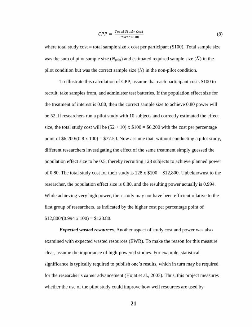
(8)

where total study cost = total sample size x cost per participant ($100). Total sample size

was the sum of pilot sample size (Npilot) and estimated required sample size ( ) in the

pilot condition but was the correct sample size (N) in the non-pilot condition.

To illustrate this calculation of CPP, assume that each participant costs $100 to

recruit, take samples from, and administer test batteries. If the population effect size for

the treatment of interest is 0.80, then the correct sample size to achieve 0.80 power will

be 52. If researchers run a pilot study with 10 subjects and correctly estimated the effect

size, the total study cost will be (52 + 10) x $100 = $6,200 with the cost per percentage

point of $6,200/(0.8 x 100) = $77.50. Now assume that, without conducting a pilot study,

different researchers investigating the effect of the same treatment simply guessed the

population effect size to be 0.5, thereby recruiting 128 subjects to achieve planned power

of 0.80. The total study cost for their study is 128 x $100 = $12,800. Unbeknownst to the

researcher, the population effect size is 0.80, and the resulting power actually is 0.994.

While achieving very high power, their study may not have been efficient relative to the

first group of researchers, as indicated by the higher cost per percentage point of

$12,800/(0.994 x 100) = $128.80.

Expected wasted resources. Another aspect of study cost and power was also

examined with expected wasted resources (EWR). To make the reason for this measure

clear, assume the importance of high-powered studies. For example, statistical

significance is typically required to publish one’s results, which in turn may be required

for the researcher’s career advancement (Hojat et al., 2003). Thus, this project measures

whether the use of the pilot study could improve how well resources are used by

22

measuring expected wasted resources. If one considers the Type II error rate to be the

probability that the resources invested in the study will be wasted, the expected wasted

resources could be defined as follows:

(9)

where the Type II error rate (β) is 1 – resulting power in the pilot condition, and 1 - 0.8 =

0.2 in the non-pilot condition.

Assume the following research scenario: each participant costs $100 and the

population effect size for the treatment of interest is 0.5. One research group used a pilot

study of 10 subjects to correctly estimate the population effect size and planned their

study accordingly to achieve 0.80 power. The total study cost for this group will be (128

+ 10) x $100 = $13,800 with wasted resources of $13,800 x (1 - 0.8) = $2,760. Another

group of researchers intuitively assumed the population effect size to be 0.80, and

planned their study with the total cost of 52 x 100 = $5,200. Unbeknownst to the

researchers, the population effect size is 0.5, and the resulting power actually is only

0.442. Thus, the researchers’ expected wasted resources would be $5,200 x (1 - 0.442) =

$2901, or more than half of their resources in such studies in the long run!

23

Chapter 4

Experiment 1

Method

In this project two separate experiments were conducted. Experiment 1 examined

the effect of conducting pilot studies with various estimation methods. The basic logic of

the study is schematized for the pilot condition in Figure 4.1, and that for the non-pilot

condition in Figure 4.2. In the pilot condition, the number of cells will be 60 = 4

(Population Effect Size δ: 0, 0.2, 0.5, 0.8) x 3 (Pilot-Study Sample Size Npilot: 6, 10, 30) x

5 (Estimation methods (the five methods are defined in the next section)), in each of

which 10,000 simulations were run. In the non-pilot condition, the number of cells will

be 12 = 4 (Population Effect Size δ: 0, 0.2, 0.5, 0.8) x 3 (Required Sample Size for

Detecting Effect Size of 0.2, 0.5, 0.8: 788, 128, 52). Thus, a total of 60+12 = 72 cells

were examined.

Effect size estimation methods. Experiment 1 used five estimation methods as

independent variables (Cohen’s d, Hedges, Wherry, Maxwell-Delaney [MD], Upper One-

Sided Confidence limit [UCL]).8 Because Cohen’s d is known to be a biased estimator of

δ (Hedges & Olkin, 1985; Hunter & Schmidt, 2004), methodologists recommend that

researchers “correct” Cohen’s d obtained from a pilot study before using it for sample-

size calculation (Maxwell & Delaney, 2004; Thompson, 2002), even though some

caution against this practice because of possible overcorrection (Roberts & Henson,

2002). While about 10 estimation methods have been proposed, this project picks three

popular estimation methods – Hedges, Wherry, and Maxwell-Delaney – to examine

8 In this project all observed effect sizes were denoted as d, regardless of estimation methods

used. This is to simplify notation even though all d’s, whether “corrected” or not, are estimates of

the population effect size which might have been denoted more formally as .

24

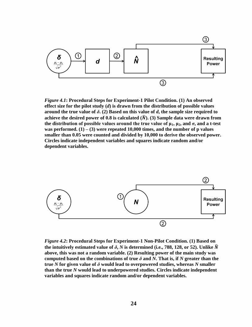
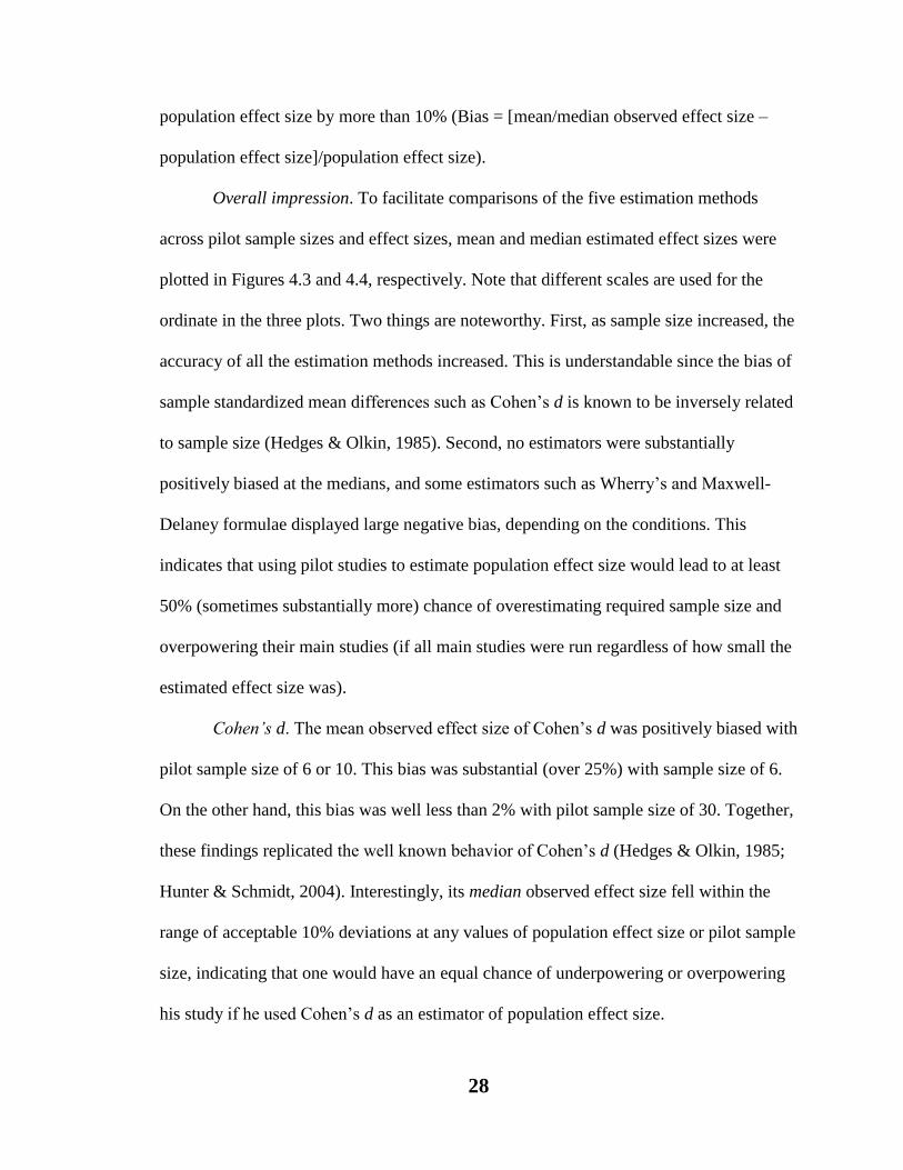
Figure 4.1: Procedural Steps for Experiment-1 Pilot Condition. (1) An observed

effect size for the pilot study (d) is drawn from the distribution of possible values

around the true value of δ. (2) Based on this value of d, the sample size required to

achieve the desired power of 0.8 is calculated ( ). (3) Sample data were drawn from

the distribution of possible values around the true value of μ1, μ2, and σ, and a t-test

was performed. (1) – (3) were repeated 10,000 times, and the number of p values

smaller than 0.05 were counted and divided by 10,000 to derive the observed power.

Circles indicate independent variables and squares indicate random and/or

dependent variables.

Figure 4.2: Procedural Steps for Experiment-1 Non-Pilot Condition. (1) Based on

the intuitively estimated value of δ, N is determined (i.e., 788, 128, or 52). Unlike

above, this was not a random variable. (2) Resulting power of the main study was

computed based on the combinations of true δ and N. That is, if N greater than the

true N for given value of δ would lead to overpowered studies, whereas N smaller

than the true N would lead to underpowered studies. Circles indicate independent

variables and squares indicate random and/or dependent variables.

25

whether applying an estimation method improves effect-size estimation in small-scale

pilot studies, and whether one performs better than the others.

Hedges formula. Hedges and Olkin (1985) discovered that Cohen’s d (originally

called g) was greater than its population counterpart δ approximately by 3δ/(4N-9) (p.

80). Thus, to correct for this bias, they proposed the following formula:

. (10)

Wherry formula The Wherry formula was originally proposed to adjust R2, and is

currently implemented in commonly used statistical packages as part of the standard

output for regression analyses (Yin & Fan, 2001). Correlational indices such as R2

are

biased and Cohen’s d can be converted into and from these indices (Roberts & Henson,

2002). Therefore, some researchers recommended that the Wherry formula be applied to

“shrink” the positive bias of Cohen’s d (e.g., Thompson, 2002). This adjustment is

achieved by first converting Cohen’s d into R2. The Wherry formula is then applied to R

2

to produce , which is subsequently converted back into .

.

(11)

Notice that this formula does not allow to have negative values. Whenever

becomes

less than 0, mainly due to sampling errors (Schmidt & Hunter, 1999), is replaced with

0.

Maxwell-Delaney (MD) formula. The MD formula was introduced to correct the

bias inherent in estimating the proportion of population variance accounted for by the

independent variable in analyses of variance when working with data from small samples

26

(Maxwell & Delaney, 2004). The original formula (p.125) estimates f from an F ratio, as

it was designed for use in one-way ANOVA where typically more than two groups would

be employed. Here, the formula is modified to estimate from a t-ratio:

. (12)

Whenever the t2 value was less than 1, is replaced with 0.

Upper one-sided confidence limit (UCL). Alternatively, techniques have been

proposed to estimate σ2 from pilot data (e.g., Browne, 1995, 2001; Julious & Owen,

2006; Shiffler & Adams, 1987). In these techniques σ2 is typically overestimated from

measures of variability such as s2 (Browne, 1995) for the following reasons. First,

because the sampling distribution of s2 of small pilot studies is positively skewed, s

2

would be smaller than σ2

more than 50% of the time. Therefore, if one were to use the

pilot s2 directly to estimate σ

2, observed power would be lower than planned power more

than 50% of the time Second, the distribution of s2

with small N is very wide, resulting in

imprecise estimation of σ2. To alleviate these difficulties in estimating σ

2, proposed

techniques of using s2 as an estimator of σ

2 involve multiplying s

2 by a certain factor, and

this factor increases as the sample size of the pilot study decreases. As an example of

such a multiplying factor, Browne proposed to use the upper one-sided confidence limit

(UCL) of pilot s2 (Browne, 1995). Because the UCL of s

2 is greater than s

2 itself, it is

most likely to prevent underestimation of required sample size and power deficits.

The current study employed a series of Monte Carlo simulations to investigate the

effect of varying sample sizes of pilot studies and various effect-size estimation methods

on the accuracy and precision of sample-size estimation and power. Specifically, three

pilot sample sizes (NPilot: 6, 10, 30) and five estimation methods (Cohen’s d, Hedges,

27

Wherry, Maxwell-Delaney, UCL) were crossed with three population effect sizes (δ: 0.2,

0.5, 0.8), and measures of central tendency and variability of observed effect size (d) and

power deviation (observed power – 0.8) were examined.

Results

Observed effect size. Descriptive statistics for the performance of the estimation

methods at the varying sample sizes are presented in Table 4.1. Each row summarizes

descriptive statistics (the mean, the standard deviation, the median, the interquartile

range, and maximum and minimum values) of a given estimation method across 10,000

replications at each combination of pilot sample size and population effect size.

Table 4.1: Descriptive Statistics for Estimated Effect Size in Experiment 1

Note. M = mean, SD = standard deviation, Mdn = median, IQR = interquartile range, MD

= Maxwell-Delaney formula, UCL = Upper Confidence Limit, δ = population effect size,

NPilot = pilot sample size.

Measures of accuracy of effect-size estimation. In this analysis, a biased

estimator is defined as an estimation method whose mean or median deviated from the

Estimation

Method

δ = .2 δ = .5 δ = .8

M (SD) Mdn (IQR) Min/Max M (SD) Mdn (IQR) Min/Max M (SD) Mdn (IQR) Min/Max

Npilot = 6

Cohen's d .25 (1.21) .21 (1.21) -9.5/22.8

.63 (1.24) .54 (1.25) -29.4/14.0

.97 (1.27) .83 (1.28) -5.7/25.7

Hedges .20 (.97) .16 (.97) -7.6/18.3

.50 (1.00) .43 (1.00) -23.5/11.2

.78 (1.01) .66 (1.03) -4.5/20.6

Wherry .38 (.84) .00 (.48) .0/20.4

.49 (.94) .00 (.75) .0/26.3

.66 (1.05) .00 (1.08) .0/23.0

MD .50 (.95) .00 (.79) .0/22.8

.64 (1.06) .00 (1.02) .0/29.4

.83 (1.18) .39 (1.34) .0/25.7

UCL .09 (.42) .07 (.42) -3.3/7.8

.22 (.43) .18 (.43) -10.1/4.8

.33 (.43) .28 (.44) -1.9/8.8

Npilot = 10

Cohen's d .22 (.73) .20 (.90) -3.6/4.5

.56 (.75) .52 (.92) -2.9/5.2

.88 (.78) .82 (.95) -2.4/5.9

Hedges .20 (.66) .18 (.81) -3.3/4.1

.51 (.68) .47 (.83) -2.6/4.7

.80 (.70) .74 (.86) -2.2/5.3

Wherry .26 (.48) .00 (.39) .0/4.2

.39 (.60) .00 (.70) .0/4.9

.62 (.73) .41 (1.07) .0/5.5

MD .31 (.52) .00 (.52) .0/4.5

.46 (.64) .00 (.81) .0/5.2

.70 (.77) .54 (1.17) .0/5.8

UCL .12 (.41) .11 (.50) -2.0/2.5

.31 (.42) .29 (.51) -1.6/2.9

.49 (.43) .46 (.53) -1.3/3.3

Npilot = 30

Cohen's d .21 (.38) .20 (.50) -1.4/2.6

.52 (.38) .51 (.50) -1.1/2.2

.82 (.40) .81 (.51) -.7/2.6

Hedges .20 (.37) .20 (.49) -1.4/2.5

.50 (.37) .49 (.48) -1.0/2.1

.80 (.39) .79 (.50) -.6/2.5

Wherry .17 (.28) .00 (.31) .0/2.5

.38 (.38) .33 (.65) .0/2.1

.70 (.44) .70 (.58) .0/2.5

MD .18 (.28) .00 (.33) .0/2.6

.40 (.39) .35 (.67) .0/2.2

.72 (.44) .72 (.59) .0/2.6

UCL .16 (.30) .16 (.39) -1.1/2.0 .40 (.30) .39 (.39) -.8/1.7 .63 (.31) .62 (.40) -.5/2.0

28

population effect size by more than 10% (Bias = [mean/median observed effect size –

population effect size]/population effect size).

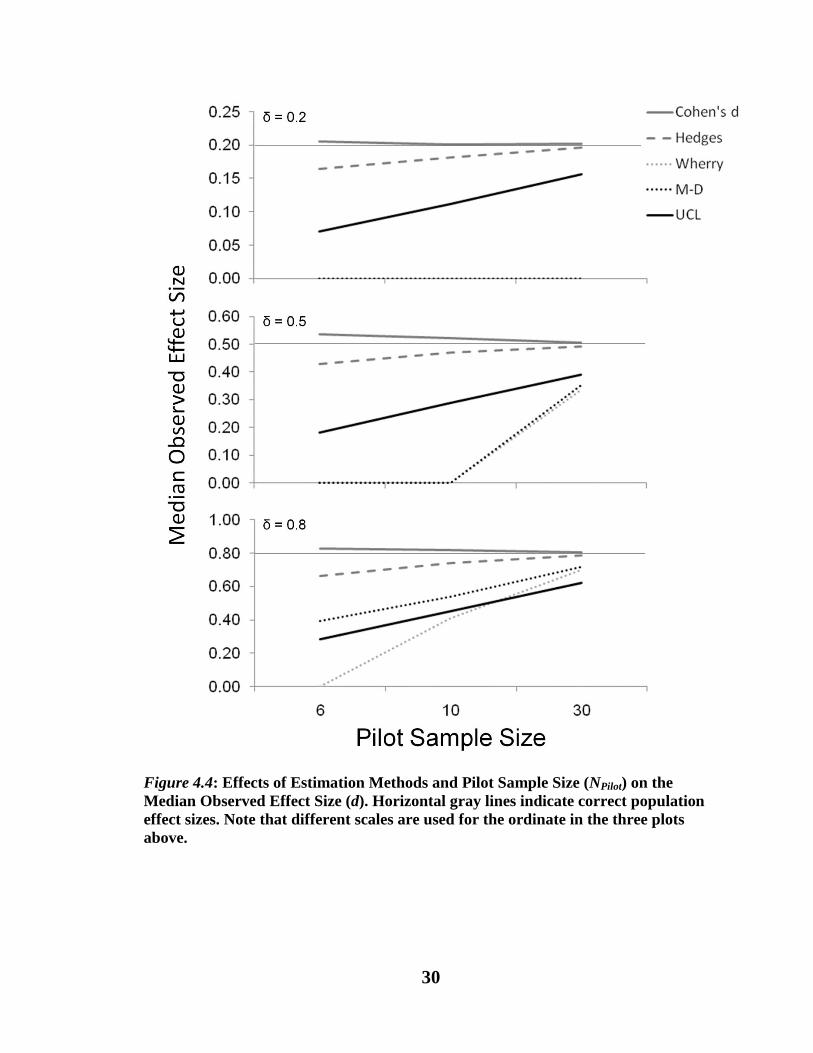
Overall impression. To facilitate comparisons of the five estimation methods

across pilot sample sizes and effect sizes, mean and median estimated effect sizes were

plotted in Figures 4.3 and 4.4, respectively. Note that different scales are used for the

ordinate in the three plots. Two things are noteworthy. First, as sample size increased, the

accuracy of all the estimation methods increased. This is understandable since the bias of

sample standardized mean differences such as Cohen’s d is known to be inversely related

to sample size (Hedges & Olkin, 1985). Second, no estimators were substantially

positively biased at the medians, and some estimators such as Wherry’s and Maxwell-

Delaney formulae displayed large negative bias, depending on the conditions. This

indicates that using pilot studies to estimate population effect size would lead to at least

50% (sometimes substantially more) chance of overestimating required sample size and

overpowering their main studies (if all main studies were run regardless of how small the

estimated effect size was).

Cohen’s d. The mean observed effect size of Cohen’s d was positively biased with

pilot sample size of 6 or 10. This bias was substantial (over 25%) with sample size of 6.

On the other hand, this bias was well less than 2% with pilot sample size of 30. Together,

these findings replicated the well known behavior of Cohen’s d (Hedges & Olkin, 1985;

Hunter & Schmidt, 2004). Interestingly, its median observed effect size fell within the

range of acceptable 10% deviations at any values of population effect size or pilot sample

size, indicating that one would have an equal chance of underpowering or overpowering

his study if he used Cohen’s d as an estimator of population effect size.

29

Figure 4.3: Effects of Estimation Methods and Pilot Sample Size (NPilot) on the Mean

Observed Effect Size (d). Horizontal gray lines indicate correct population effect

sizes. Note that different scales are used for the ordinate in the three plots above.

30

Figure 4.4: Effects of Estimation Methods and Pilot Sample Size (NPilot) on the

Median Observed Effect Size (d). Horizontal gray lines indicate correct population

effect sizes. Note that different scales are used for the ordinate in the three plots

above.

31

Hedges’ formula. The mean observed effect size of the Hedges’ formula was

unbiased at any levels of the independent variables. On the other hand, its median was

negatively biased with sample size of 6 at all effect sizes, indicating that more than 50%

of the main studies would be overpowered.

Wherry’s formula. The mean observed effect size was positively biased at effect

size of 0.2: the means were 0.377 and 0.255 with pilot sample sizes of 6 and 10,

respectively. This was because Wherry’s formula does not allow observed effect size to

take any negative values. That is, all negative values were converted to 0, which in turn

were shifting the mean upward. In the other conditions, the mean of Wherry’s formula

resulted in negative bias, ranging from -13.1% to -23.6%. At the median, Wherry’s

formula resulted in gross underestimation. Specifically, all the median observed effect

sizes were 0, except for two conditions (at effect size of 0.5 with sample size of 30 and

effect size of 0.8 with sample sizes of 10 and 30). This could be very problematic for

researchers because too small an observed effect size may lead them to abort their main

studies (Algina & Olejnik, 2003; Kraemer et al., 2006). With Wherry’s formula, that

could happen more than 50% of the time in many of the situations examined.

Maxwell-Delaney (MD) formula. Similar to the results in Wherry’s formula, the

mean observed effect size was positively biased: at population effect size of 0.2, the

means were 0.53 and 0.306 with pilot sample sizes of 6 and 10, respectively, and at effect

size of 0.5, the mean was 0.635 with sample size of 6. This was because the MD formula,

given it was designed for use with any number of groups, does not allow observed effect

size to take any negative values. In the other conditions, the formula resulted in negative

32

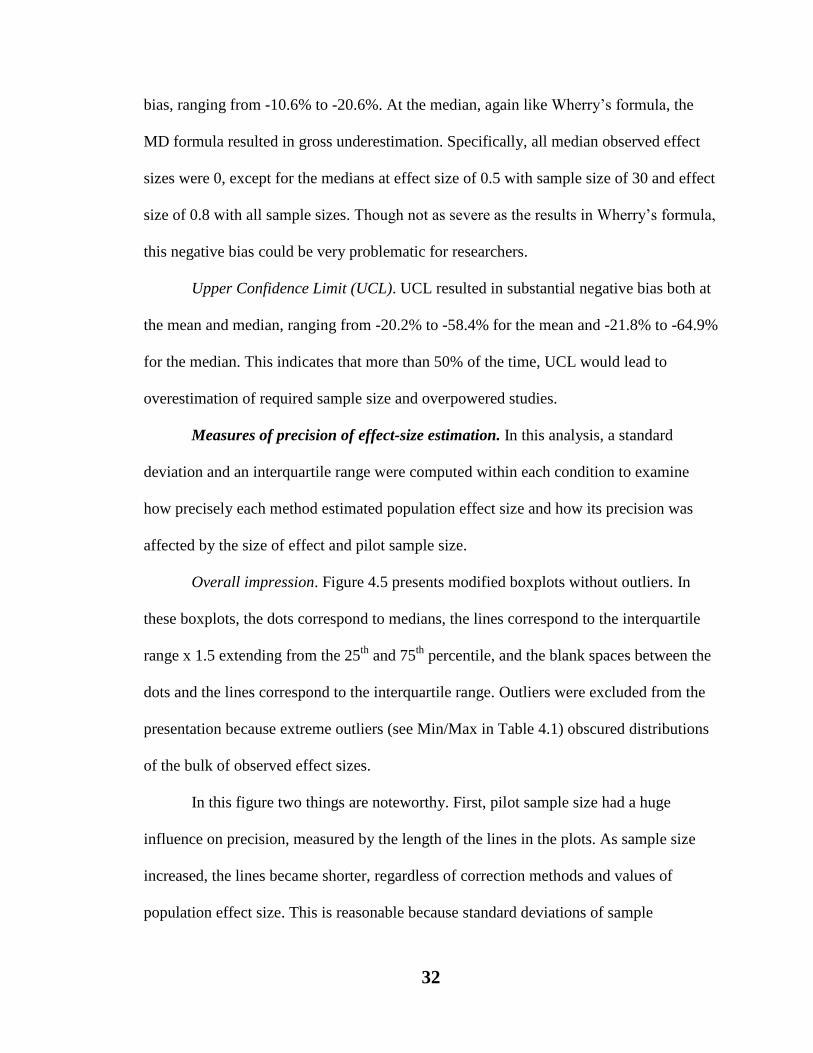
bias, ranging from -10.6% to -20.6%. At the median, again like Wherry’s formula, the

MD formula resulted in gross underestimation. Specifically, all median observed effect

sizes were 0, except for the medians at effect size of 0.5 with sample size of 30 and effect

size of 0.8 with all sample sizes. Though not as severe as the results in Wherry’s formula,

this negative bias could be very problematic for researchers.

Upper Confidence Limit (UCL). UCL resulted in substantial negative bias both at

the mean and median, ranging from -20.2% to -58.4% for the mean and -21.8% to -64.9%

for the median. This indicates that more than 50% of the time, UCL would lead to

overestimation of required sample size and overpowered studies.

Measures of precision of effect-size estimation. In this analysis, a standard

deviation and an interquartile range were computed within each condition to examine

how precisely each method estimated population effect size and how its precision was

affected by the size of effect and pilot sample size.

Overall impression. Figure 4.5 presents modified boxplots without outliers. In

these boxplots, the dots correspond to medians, the lines correspond to the interquartile

range x 1.5 extending from the 25th

and 75th

percentile, and the blank spaces between the

dots and the lines correspond to the interquartile range. Outliers were excluded from the

presentation because extreme outliers (see Min/Max in Table 4.1) obscured distributions

of the bulk of observed effect sizes.

In this figure two things are noteworthy. First, pilot sample size had a huge

influence on precision, measured by the length of the lines in the plots. As sample size

increased, the lines became shorter, regardless of correction methods and values of

population effect size. This is reasonable because standard deviations of sample

33

Figure 4.5: Effects of Estimation Methods and Pilot Sample Size (NPilot) on the

Distribution of Observed Effect Size (d) in Experiment 1.

34

standardized mean differences such as Cohen’s d are known to be inversely related to

sample size (Hedges & Olkin, 1985). Even though the sampling distributions of the

interquartile ranges of Cohen’s d and the other estimators are not known, it is reasonable

to assume that it behaves similar to their standard deviations. Second, Wherry and

Maxwell-Delaney formula displayed asymmetric distributions in many conditions: when

the median sat at 0, there were no lines extending downward from the median. This is

because these formulae did not allow negative values, which were all converted to 0.

In addition, one can compare the widths of the standard deviations and

interquartile ranges in Table 4.1. While the widths of the standard deviations and

interquartile ranges were similar with sample size of six, regardless of estimation

methods and population effect size, the standard deviations became narrower than the

ranges as sample size grew. This is probably because some pilot studies with small

sample size yielded extreme values of observed effect size, inflating the standard

deviation (e.g., Max[dNPilot=6] = 4.8~29.4). On the other hand, these extreme values

disappeared as sample size increased (Max[dNPilot=30] = 1.7~2.6), making the standard

deviation much narrower.

Cohen’s d. Cohen’s d turned out to be the least precise estimation method in

terms of both measures of precision: it had the widest standard deviation and interquartile

range across all sample sizes and effect sizes (see Table 4.1 and Figure 4.5). While its

precision improved as sample size increased, its estimation was still less precise than

other estimators in most cases.

Hedges’ formula and UCL. Hedges’ formula estimated population effect size

consistently more precisely than Cohen’s d, indicated by its narrower standard deviations

35

and interquartile ranges. This is understandable because the values of the observed effect

size based on Hedges’ formula were obtained by shrinking Cohen’s d, thereby narrowing

its standard deviation as well. Likewise, the UCL, which shrinks Cohen’s d to a much

greater extent than Hedges’ formula, displayed narrower standard deviations and

interquartile ranges.

Wherry and MD formulae. Because the distributions of observed effect size

estimated by Wherry’s and MD formulae were not symmetric, interpreting measures of

variability such as standard deviation and interquartile range that assumes some degree of

symmetric distributions is not meaningful, especially given the median observed effect

size was 0.

Ninety-five percent confidence interval around observed effect size.

Methodologists increasingly highlight the importance of precision as well as accuracy of

effect-size estimation (Kelley, 2005; Maxwell et al., 2008). Consequently, researchers are

advised or are in some instances required to report confidence intervals around the

estimated effect size, while a smaller emphasis is placed on p values and test statistics

(Algina & Keselman, 2003; Cummings, 2007). Even in the case of pilot studies, it may

be useful for researchers to be aware of how precise or imprecise small pilot studies

estimate population effect size. Therefore, how different effect-size estimation methods

and pilot sample size modified the width of 95% confidence interval (CI95) was

examined.

To obtain empirical distributions of CI95’s, a CI95 for each observed effect size

in a pilot study was obtained using an R package MBESS (Kelley & Lai, 2010). One of

the functions implemented in the package, ci.smd(), computes a CI95 around a

36

standardized mean difference such as Cohen’s d by first estimating a non-centrality

parameter for the t test (λ) using the sample mean, the standard deviation, and the sample

size. Then, it forms a CI95 around the λ, and finally estimates a CI95 for the population

effect size δ by dividing the upper and lower confidence limits around the λ by the square

root of the sample size. The width of the CI95 (upper confidence limit – lower confidence

limit) was used as the dependent variable in this analysis.

Table 4.2 summarizes the descriptive statistics for the width of the CI95. For each

combination of population effect size and pilot sample size, the “correct” width is shown;

that is, if an observed effect size matches its population counterpart, the observed width

would match the correct width. The correct width is inversely related with sample size

but positively related with population effect size.

Table 4.2: Descriptive Statistics for 95% Confidence Intervals around Observed Effect

Size in Experiment 1


= Maxwell-Delaney formula, UCL = Upper Confidence Limit, δ = population effect size

NPilot = pilot sample size.

Estimation

Method

δ = .2 δ = .5 δ = .8


Npilot = 6

CI Correct Width = 3.21



Cohen's d 3.52 (.74) 3.31 (.32) 3.2/29.5

3.60 (.83) 3.35 (.42) 3.2/37.8

3.73 (.93) 3.42 (.57) 3.2/33.2

Hedges 3.42 (.55) 3.27 (.21) 3.2/24.3

3.48 (.61) 3.29 (.27) 3.2/30.3

3.56 (.68) 3.34 (.38) 3.2/26.6

Wherry 4.29 (.67) 4.53 (.50) 3.2/26.4

4.28 (.71) 4.53 (.72) 3.2/33.8

4.24 (.78) 4.53 (.91) 3.2/29.7

MD 4.25 (.76) 4.53 (.87) 3.2/29.4

4.24 (.82) 4.53 (.93) 3.2/37.8

4.22 (.89) 4.53 (.98) 3.2/33.1

UCL 3.25 (.16) 3.21 (.04) 3.2/10.8

3.26 (.17) 3.22 (.05) 3.2/13.7

3.28 (.19) 3.23 (.07) 3.2/12.1

Npilot = 10




Cohen's d 2.58 (.17) 2.52 (.11) 2.5/5.0

2.63 (.23) 2.55 (.18) 2.5/5.6

2.71 (.30) 2.61 (.28) 2.5/6.1

Hedges 2.56 (.14) 2.51 (.09) 2.5/4.6

2.60 (.19) 2.53 (.14) 2.5/5.2

2.67 (.25) 2.58 (.23) 2.5/5.7

Wherry 2.83 (.17) 2.92 (.20) 2.5/4.7

2.82 (.20) 2.92 (.28) 2.5/5.3

2.82 (.25) 2.92 (.30) 2.5/5.8

MD 2.82 (.19) 2.92 (.27) 2.5/5.0

2.81 (.22) 2.92 (.30) 2.5/5.5

2.82 (.27) 2.92 (.31) 2.5/6.1

UCL 2.51 (.06) 2.49 (.04) 2.5/3.5

2.53 (.08) 2.50 (.06) 2.5/3.7

2.56 (.11) 2.52 (.09) 2.5/4.0

Npilot = 30




Cohen's d 1.45 (.03) 1.44 (.02) 1.4/2.0

1.47 (.04) 1.46 (.05) 1.4/1.8

1.51 (.06) 1.49 (.08) 1.4/2.0

Hedges 1.45 (.03) 1.44 (.02) 1.4/2.0

1.47 (.04) 1.45 (.04) 1.4/1.8

1.50 (.06) 1.49 (.07) 1.4/1.9

Wherry 1.48 (.03) 1.50 (.04) 1.4/2.0

1.48 (.04) 1.49 (.04) 1.4/1.8

1.50 (.06) 1.50 (.06) 1.4/1.9

MD 1.48 (.03) 1.50 (.04) 1.4/2.0

1.48 (.04) 1.49 (.04) 1.4/1.8

1.50 (.06) 1.50 (.06) 1.4/2.0

UCL 1.44 (.02) 1.44 (.01) 1.4/1.8 1.45 (.03) 1.45 (.03) 1.4/1.7 1.48 (.04) 1.47 (.05) 1.4/1.8

37

With pilot sample size of 30, all estimators performed similarly well: their means

and medians were less than 3% away from the correct values, and their standard

deviations and interquartile ranges were all less than 0.08. With smaller sample sizes, the

UCL method performed consistently better than the rest of the methods. Specifically, the

means and medians of the UCL’s CI widths had the smallest deviations from the correct

CI widths, and the UCL’s distribution of CI widths had the smallest standard deviations

and interquartile ranges. Keep it in mind that, even though the UCL method produced

confidence intervals that were narrower than those produced by the other methods, its

point estimation was negatively biased by 20 to 65%.

On the other hand, Wherry and MD did not perform as well as the other three

with pilot sample sizes of 6 and 10. Wherry had the mean CI widths furthest away from

the correct values, while the distribution of MD CI widths had the widest standard

deviations and interquartile ranges. These results may be because these two estimators

convert so many observed effect sizes into 0’s. The width of CI95 at an effect size of 0 is

4.534, which is far away from any of the correct values.

In any case, these results together demonstrate how imprecise the estimation of

population effect size using pilot studies can be. Even in the best case scenario of

population effect size of 0.8, pilot sample size of 30, and the best estimator UCL, the

mean width was 1.48, far larger than the effect size itself and reaching below 0.10. These

results together are consistent with the notion that precise estimation of population effect

size requires study design qualitatively different from a design to maximize power of an

individual study, and that it typically requires hundreds of subjects, if not thousands

38

(Kelley et al., 2003). It is impossible to achieve precise estimation of population effect

size in small pilot studies.

Estimated required sample size. Based on the observed effect sizes obtained

initially, estimated required sample sizes ( ) for achieving power of 0.8 at α = 0.05 were

calculated. One of the concerns in using pilot studies to estimate required sample size for

the main studies is that, because the sampling distribution of observed effect size with

small sample size is so wide, a certain proportion of estimated effect sizes can be so small

that the estimated required sample size must be impractically large to achieve desired

power. Even worse, if the observed effect size is zero, the required sample size will be

infinity (Algina & Olejnik, 2003; Kraemer et al., 2006). Therefore, the minimum

observed effect size estimated by any of the five estimation methods was set at 0.05; that

is, when a simulated pilot study yielded an estimated effect size below this threshold, the

population effect size was deemed too small. As a consequence, the corresponding main

study was aborted, expressed by an NA (Kraemer et al., 2006). This value of 0.05 was

chosen for two reasons. First, an effect size of 0.05 requires a sample size (N) of 12,562

to achieve power of 0.8. While large multi-center clinical trials with over 10,000 subjects

are presently not unusual, only the best funded research projects can achieve such a huge

sample size. Thus, even though observed effect size of 0.05, equivalent to point biserial

correlation of 0.025, can be practically significant in some situations (e.g., a 2.5

percentage points reduction in mortality rate, Rosenthal & Rosnow, 1985), such a small

effect size may be deemed too small in most social scientific applications, especially

given the huge required sample size. Second, this value of 0.05 could represent the

practical lower limit to the threshold of observed effect size estimated in a small pilot

39

study. That is, if the threshold of observed effect size were higher, many more main

studies would be aborted, as Kraemer and colleagues set the threshold at 0.5 (Kraemer et

al., 2006). Such a high value may be unreasonable especially when the purpose of the

main study was exploratory or when one would expect a small population effect size. If

the threshold of observed effect size were set to values lower than 0.05, such as 0, fewer

studies would be aborted. Yet, some pilot studies would yield observed effect size so low

that estimated required sample size would be astronomical (e.g., at observed effect size of

0.005, estimated required sample size would be over 120,000!). In addition, adopting the

procedure described in Kraemer and colleague’s study (2006), all negative observed

effect sizes led to aborted main studies, even though they might have been large enough

in absolute value. This is because, even though detecting and publishing the harm of a

particular treatment is important (e.g., Rothstein et al., 2005; Turner et al., 2008), seeing a

negative treatment effect at the pilot stage would discourage researchers from carrying

out their main study.

Because some cases had NA’s in the required-sample size column, the

distributions of estimated required sample size was a mixture of two variables:

categorical (NA’s) and numeric (non-NA values ranging from 2 to 12,562). Thus, this

variable did not allow the mean and the standard deviation as measures of central

tendency and variability; instead, five percentile points (10th

, 25th

, 50th

, 75th

, and 90th

)

were computed. These points allow readers to extract the median (the 50th

percentile) and

interquartile range (75th

percentile – 25th

percentile).

Overall impression. Table 4.3 presents the five percentile points of estimated

required sample sizes ( ) at each level of the five estimation methods and three

40

population effect sizes along with correct sample size to achieve power of 0.8. The first

striking impression is that there are many cells with NA’s in the table. In some

conditions, NA’s appeared even at the 50th

percentile (the median), indicating that pilot

studies in those conditions yielded observed effect size below the threshold of 0.05,

which led to aborting their main studies in more than 50% of the 10,000 replications. The

second impression is that in general estimated required sample sizes were far below the

correct sample size. For instance, at population effect size of 0.2, the correct sample size

to achieve power of 0.8 is 788. Nevertheless, none of the estimation methods with any of

the pilot sample sizes reached that sample size at the 75th

percentile. Only at the 90th

percentile did some estimation methods reach that value. This gap between estimated and

Table 4.3: Quantiles of the Distribution of Estimated Required Sample Size in

Experiment 1

Note. NA indicates that the main study was aborted because of too small or negative

observed effect size (d < 0.05), MD = Maxwell-Delaney formula, UCL = Upper

Confidence Limit, δ = population effect size, NPilot = pilot sample size.

Estimation

Method

δ = .2 (N = 788) δ = .5 (N = 128) δ = .8 (N = 52)

10 / 25 / 50 / 75 / 90 10 / 25 / 50 / 75 / 90 10 / 25 / 50 / 75 / 90

Npilot = 6

Cohen's d NA / NA / 12 / 82 / 426

NA / NA / 20 / 82 / 384

NA / 8 / 22 / 72 / 286

Hedges NA / NA / 18 / 120 / 626

NA / NA / 28 / 122 / 542

NA / 10 / 32 / 110 / 422

Wherry NA / NA / NA / 12 / 64

NA / NA / NA / 16 / 66

NA / NA / NA / 22 / 78

MD NA / NA / NA / 20 / 78

NA / NA / NA / 24 / 82

NA / NA / 8 / 26 / 82

UCL NA / NA / 40 / 464 / 1931

NA / NA / 118 / 508 / 1868

NA / 26 / 140 / 484 / 1640

Npilot = 10

Cohen's d NA / NA / 28 / 146 / 728

NA / 8 / 36 / 126 / 538

NA / 14 / 32 / 94 / 338

Hedges NA / NA / 32 / 174 / 846

NA / 8 / 44 / 152 / 632

NA / 16 / 40 / 114 / 408

Wherry NA / NA / NA / 26 / 122

NA / NA / NA / 38 / 140

NA / NA / 14 / 46 / 132

MD NA / NA / NA / 36 / 142

NA / NA / NA / 42 / 146

NA / NA / 16 / 46 / 140

UCL NA / NA / 68 / 390 / 1660

NA / NA / 102 / 354 / 1340

NA / 36 / 94 / 274 / 936

Npilot = 30

Cohen's d NA / NA / 98 / 392 / 1496

NA / 40 / 88 / 230 / 714

20 / 30 / 48 / 96 / 234

Hedges NA / NA / 104 / 412 / 1551

NA / 42 / 92 / 242 / 748

20 / 30 / 52 / 100 / 248

Wherry NA / NA / NA / 116 / 440

NA / NA / 48 / 142 / 398

NA / 24 / 48 / 100 / 240

MD NA / NA / NA / 120 / 442

NA / NA / 50 / 144 / 414

NA / 24 / 46 / 96 / 232

UCL NA / NA / 148 / 594 / 2072 NA / 64 / 142 / 374 / 1094 30 / 46 / 79 / 156 / 382

41

correct sample sizes became narrower at larger population effect sizes. Together, these

results indicate that main studies designed to detect small population effect size would be

either underpowered or aborted more than 75% of the repeated attempts if they relied on

pilot studies in estimating a small effect size. This is a replication of the results reported

in Kraemer and colleagues (2006) and Algina and Olejnik (2003), even though they used

different effect-size thresholds and different statistical tests (Kraemer and colleagues:

threshold = 0.5, one-sample t-test; Algina and Olejnik: threshold = 0, one-way ANOVA).

Cohen’s d. At a population effect size of 0.2, Cohen’s d underestimated required

sample size or led to abandonment of the main study in more than 90% of the simulated

pilot studies with pilot sample size of or 10, and in more than 75% of the studies with

pilot sample size of 30. At an effect size of 0.5, it underestimated required sample size or

led to abortion in more than 75% of the simulated studies with sample size of 6 or 10, and

more than 50% with sample size of 30. At 0.8, it still underestimated required sample size

or led to abortion in more than 50% of the simulated studies with all sample sizes.

Hedges’ formula. Hedges’ formula, proposed to correct the overestimation of

Cohen’s d, performed slightly better. At a population effect size of 0.2, it underestimated

required sample size or led to abortion of the main study in more than 90% of the

simulated pilot studies with pilot sample size of 6, and in more than 75% of the studies

with 10 or 30. At 0.5, it underestimated required sample size or led to abandonment in

more than 75% of the simulated studies with 6, and in more than 50% with 10 or 30. At δ

= 0.8, it yielded required sample size greater than the correct sample size or led to

abortion in less than 75% of the studies with pilot sample size of 6 or 10, and less than

50% of the studies with 30.

42

Wherry and MD Formulae. At a population effect size of 0.2, Wherry’s and

Maxwell-Delaney formulae underestimated required sample size or led to abandonment

of the main study in more than 90% of the simulated pilot studies with all pilot sample

sizes. Even with pilot sample size of 30, their estimated required sample sizes at the 90th

percentile were 440 and 420, respectively, far below the correct sample size of 788. At

0.5, it underestimated sample size or led to abandonment in more than 90%, 75%, and

50% of the simulated studies with pilot sample size of 6, 10, amd 30, respectively. At 0.8,

it underestimated sample size or led to abandonment in more than 75% of the simulated

studies with pilot sample size of 6 or 10, and in more than 50% with 30.

UCL. Even though the UCL led to abortions of main studies to an extent similar

to Cohen’s d and Hedges’ formula, the UCL was the only formula that overestimated

required sample size of the main study at a small population effect size. At a population

effect size of 0.2, it underestimated required sample size or led to abortion of the main

study in more than 90% of the simulated pilot studies with pilot sample size of 6, and in

more than 75% of the studies with 10 or 30. But it led overestimated sample size in more

than 10% of the time with all sample sizes. At 0.5, it underestimated required sample size

or led to abandonment in more than 75% of the simulated studies with Npilot of 6, and in

more than 50% with 10 and more than 25% with 30. It again led to overestimation of

sample size more than 25% to 50% of the time, depending on the pilot sample size. At

0.8, it yielded required sample size greater than the correct sample size or led to abortion

in less than 50% of the studies with all pilot sample sizes. It overestimated sample size in

more than 25% to 50% of the time, depending on the pilot sample size.

43

Probability of the main study being aborted. Many pilot studies yielded an

estimated effect size below the threshold of 0.05; as a result, instances of aborted main

studies were likewise pervasive. To quantify the proportion of aborted main studies to all

simulated studies, the instances of aborted studies were counted and divided by the

number of replications (10,000). Results are summarized in Figure 4.6.

Two points are noteworthy. First, Cohen’s d, Hedges’ formula, and UCL showed

similar patterns. With these methods, the probability of the main study aborted was

primarily a function of population effect size: as effect size increased, the probability

rapidly decreased from 0.35~0.45 at 0.2 to 0.05~0.2 at 0.8. Surprisingly, pilot sample size

appears to have been less of an important factor: increasing pilot sample size from 6 to 30

decreased the probability by 10~15 percentage points, a smaller reduction than the

reduction achieved by increasing population effect size from 0.2 to 0.8. Among these

three methods, Cohen’s d, with its positive bias, led to the fewest aborted main studies.

Second, Wherry’s and Maxwell-Delaney formulae showed similar patterns. At

small effect size, applying these estimation methods led to aborted main studies in more

than 60% of the simulated pilot studies, regardless of pilot sample size. Even at 0.5, more

than 40% of the studies were aborted with all pilot sample sizes. Only at the large effect

size, combined with sample size of 30, did the probability become smaller than 20%.

Power deviation. Because some main studies were aborted because observed

effect size did not reach the threshold value in their pilot counterparts, power analysis

was not straight forward. To deal with this problem, two types of power were computed:

total power and valid power. Total power was defined as: (number of main studies with p

< 0.05 / number of all simulated pilot studies). This value can be conceptualized as the

44

Figure 4.6: Probability of the Main Study being Aborted Based on Pilot Results.

45

probability of successfully rejecting the null if one chooses to conduct a pilot study to

estimate population effect size at the risk of aborting one’s main study. In other words, if

the observed effect size did not reach the threshold value and if one aborted one’s study,

it can be considered that one committed a Type II error: even though the population

effect size was greater than 0 (i.e., the null hypothesis was false), it would not be possible

to reject the false null. On the other hand, valid power is defined as: (number of main

studies with p < 0.05 / number of valid pilot studies) where a valid pilot study is defined

as a pilot study with observed effect size greater than or equal to the threshold value of

0.05, thus leading to the main study actually being carried out. This power can be

considered as the probability of successfully rejecting the null hypothesis in the main

study conditional upon the estimated effect size reaching the threshold value in a pilot

study. After these powers were computed within each condition, the power deviation was

calculated by subtracting the desired level of power of 0.8 from both powers. The value

of 0 indicates the estimated power matching the desired power, while positive and

negative values indicate overpowering and underpowering, respectively. Figures 4.7 and

4.8 summarize the result of power deviations based on total power and valid power.

Power deviation - total power. The first striking impression is the pervasiveness

of underpowered studies. This is surprising because pilot studies were designed to

estimate the population effect size so that the main studies would on average achieve

power of 0.8. (The role played by the large proportion of aborted studies in this

surprising result will be noted in the Discussion below.) The underpowering was

particularly pervasive at small population effect size: all correction methods led to

considerable underpowered main studies, regardless of pilot sample size. The worst

46

Figure 4.7: Power Deviation Derived from the Power Based on All Studies (Total

Power - 0.8).

47

Figure 4.8: Power Deviation Derived from the Power Based on Valid Studies (Valid

Power - 0.8).

48

performing estimator was Wherry’s formula, with power deviations ranging from -0.65 to

-0.75. This result may not be surprising given that so many of the main studies were

aborted if this estimator was used (see Figure 4.6), resulting in very low overall power.

Even the best performer, UCL, resulted in underpowering by ~0.5 at a small effect size.

The performance of the other estimators fell in between.

At a population effect size of 0.5, all estimators still produced considerable

numbers of underpowered main studies, yet the magnitude of underpowering was smaller

especially with large pilot sample size. The worst performing estimator was again

Wherry’s formula, with power deviations ranging from -0.35 to -0.65, while the best

performer, UCL, resulted in underpowering by 0.05 to 0.20. At a large population effect

size, performances of all correction methods continue to improve, especially when

combined with a pilot sample size of 30. With this sample size, power deviations for all

methods were less than 0.15 in absolute value, and UCL even resulted in overpowering.

Power deviation - valid power. Figure 4.8 summarizes the results of power

analysis based on valid pilot studies and resulting power deviations. Overall patterns

were similar to the patterns based on total power deviations, with all biases being shifted

upward. The mean power deviation of all 45 conditions was -0.40 for total power

deviations and -0.24 for valid power deviations. Yet, all estimation methods displayed

considerable underpowering at a population effect size of 0.2 regardless of pilot sample

size (the mean deviations of the 15 conditions at effect size of 0.2 was -0.44).

Measures of economic performance. To compute the economic efficiency of

conducting pilot studies, an index called expected wasted resources was computed as

follows. First, total sample size (pilot sample size + estimated required sample size) was

49

computed for each pair of a pilot study and its corresponding main study. If a pilot result

led to an aborted main study, pilot sample size was used as the total sample size. Second,

the total study cost was computed by multiplying the cost per subject of $100 by the total

sample size. Third, the median of the total study costs was computed across the 10,000

simulated pilot/main study pairs. This value represents the hypothetical cost of a typical

study (i.e., a pilot study with or without a main study) over many replications. The

median was used because means were inflated by outliers (with pilot sample size of 6, the

mean of max estimated required sample size across 15 conditions was 12,229). Fourth,

the median study cost was multiplied by (1 – total power) to derive expected wasted

resources within each condition. Likewise, a cost per percentage point was computed for

each condition by dividing the median total study cost by (total power * 100),

representing a typical cost of increasing power by one percentage point. Table 4.4

presents effects of pilot sample size and estimation methods on the median total study

Table 4.4: Measures of Economic Efficiency in Experiment 1

Note. Mdn Cost = Median Total Study Cost, EWR = Expected Wasted Resources, CPP =

Cost per Percentage Point, MD = Maxwell-Delaney formula, UCL = Upper Confidence

Limit, δ = population effect size, NPilot = pilot sample size.

Estimation

Method

δ = .2 δ = .5 δ = .8

Mdn Cost EWR CPP Mdn Cost EWR CPP Mdn Cost EWR CPP

NPilot = 6

Cohen's d $ 1,800 $ 1,518 $ 115

$ 2,600 $ 1,726 $ 77

$ 2,800 $ 1,420 $ 57

Hedges $ 2,400 $ 1,965 $ 133

$ 3,400 $ 2,067 $ 87

$ 3,800 $ 1,668 $ 68

Wherry $ 600 $ 571 $ 125

$ 600 $ 517 $ 43

$ 600 $ 449 $ 24

MD $ 600 $ 565 $ 104

$ 600 $ 498 $ 35

$ 1,400 $ 1,001 $ 49

UCL $ 4,600 $ 3,240 $ 156

$ 12,400 $ 5,423 $ 220

$ 14,600 $ 4,004 $ 201

NPilot = 10

Cohen's d $ 3,800 $ 3,045 $ 191

$ 4,600 $ 2,657 $ 109

$ 4,200 $ 1,753 $ 72

Hedges $ 4,200 $ 3,302 $ 196

$ 5,400 $ 2,950 $ 119

$ 5,000 $ 1,911 $ 81

Wherry $ 1,000 $ 929 $ 141

$ 1,000 $ 787 $ 47

$ 2,400 $ 1,507 $ 65

MD $ 1,000 $ 922 $ 129

$ 1,000 $ 772 $ 44

$ 2,600 $ 1,588 $ 67

UCL $ 7,800 $ 5,579 $ 274

$ 11,200 $ 4,804 $ 196

$ 10,400 $ 2,418 $ 136

NPilot = 30

Cohen's d $ 12,800 $ 8,848 $ 415

$ 11,800 $ 4,584 $ 193

$ 7,800 $ 2,107 $ 107

Hedges $ 13,400 $ 9,242 $ 432

$ 12,200 $ 4,641 $ 197

$ 8,200 $ 2,080 $ 110

Wherry $ 3,000 $ 2,574 $ 211

$ 7,800 $ 4,363 $ 177

$ 7,800 $ 2,534 $ 116

MD $ 3,000 $ 2,541 $ 196

$ 8,000 $ 4,470 $ 181

$ 7,600 $ 2,516 $ 114

UCL $ 17,800 $ 11,454 $ 499 $ 17,200 $ 5,048 $ 243 $ 10,900 $ 1,725 $ 129

50

cost, expected wasted resources, and cost per percentage point at each effect size.

To depict the relationship among the variables, expected wasted resources were

plotted in Figure 4.9. Three things are note worthy. First, as population effect size

increased from 0.2 to 0.8, overall expected wasted resources decreased. This is because,

at a large effect size, fewer subjects were required to achieve high power than at smaller

effect sizes. Second, as pilot sample size increased from 6 to 30, expected wasted

resources in general increased (except for UCL with sample size of 10 and 30 at effect

sizes of 0.5 and 0.8). This may appear counterintuitive because as pilot sample size

increased, estimated required sample size increased as well (Table 4.3), which in turn

improved power (Figures 4.7 and 4.8). Yet, this positive relationship between pilot

sample size and expected wasted resources make sense because the improvement in

power was not as rapid as the increase in the total study cost. For example, at the small

effect size, Cohen’s d achieved total power of only 0.199 based on a pilot sample of 10,

and its median total study cost was $3,800. With a sample size of 30, its study cost

increased more than 200% to $12,800, yet the corresponding power increase was only

55% to 0.309. The third impression is that the UCL method yielded the greatest expected

wasted resources whereas Wherry’s formula yielded the smallest (mean expected wasted

resources over the nine conditions: UCL = $4,855; Wherry = $1,581). Also in UCL, pilot

sample size was inversely related to expected wasted resources at effect sizes of 0.5 and

0.8, while in the other four methods, the relationship was positive. This is because total

power improved for UCL as pilot sample size increased (i.e., fewer main studies were

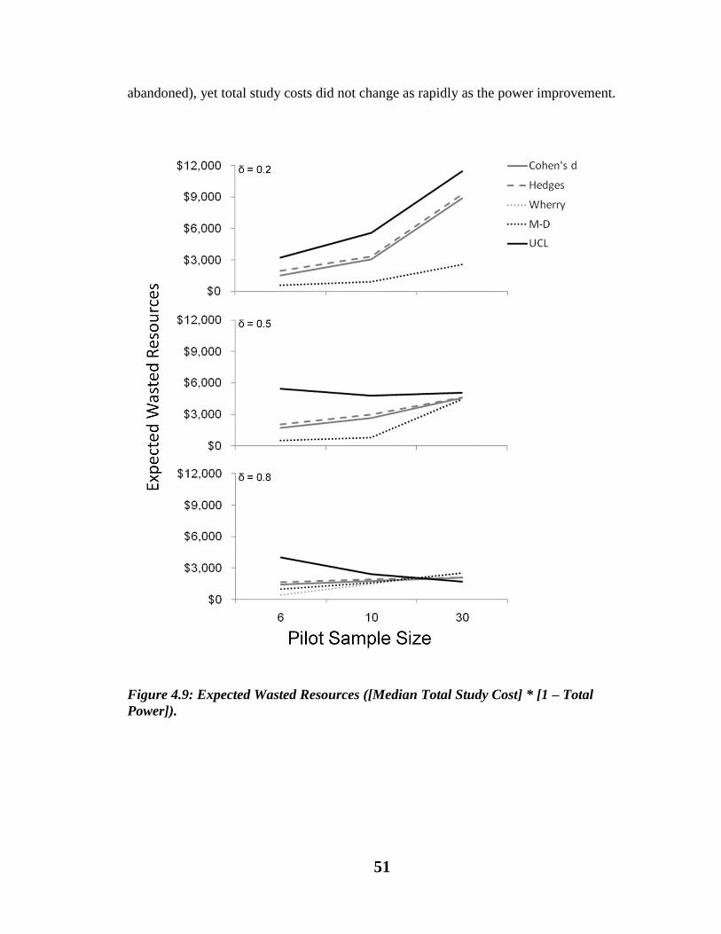
51

abandoned), yet total study costs did not change as rapidly as the power improvement.

Figure 4.9: Expected Wasted Resources ([Median Total Study Cost] * [1 – Total

Power]).

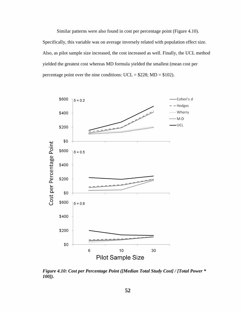
52

Similar patterns were also found in cost per percentage point (Figure 4.10).

Specifically, this variable was on average inversely related with population effect size.

Also, as pilot sample size increased, the cost increased as well. Finally, the UCL method

yielded the greatest cost whereas MD formula yielded the smallest (mean cost per

percentage point over the nine conditions: UCL = $228; MD = $102).

Figure 4.10: Cost per Percentage Point ([Median Total Study Cost] / [Total Power *

100]).

53

Power, EWR, and CCP of studies conducted without pilot studies. The

purpose of conducting a pilot study prior to a main study is to estimate the unknown

population effect size for calculating sample size necessary to achieve a desired level of

power. Yet, the above results suggest that, if a pilot study of small sample size (30 or

less) were used, the desired power was rarely achieved. Now researchers may be asking

whether they may be better off if they simply estimate population effect size based on

other criteria (e.g., based on their experience, minimally-important difference, past

publications, meta-analysis). These means of estimating effect size are advocated by

some methodologists (e.g., Kraemer et al., 2006).

Yet, some studies report that, in estimating a particular population effect size a

priori, researchers tend to underestimate the standard deviation of the effect, thereby

overestimating the effect size and underpowering their studies (Charles et al., 2009;

Vickers, 2003). That is, if a researcher recruits 788 subjects believing that the population

effect size of interest is 0.2, but if the effect size actually is 0.10 (he underestimated the

population standard deviation by 50% of its true value), his study will be severely

underpowered. In fact, the power of his study will be only 0.29, a serious power deviation

of -0.51. Yet, as we have seen, estimating small population effect size in pilot studies can

result in power deviations even more severe than -0.51 (e.g., Wherry with pilot sample

size of 6). In this case, 50% underestimation of the standard deviation (or 100% over

estimation of effect size) may still be acceptable compared with conducting a pilot study

since the latter tends to achieve even smaller power. Then, a pertinent question may be to

ask: which method of estimation would be better in achieving power close to a desired

level, conducting a pilot study, or intuitively predicting population effect size? In other

54

words, what is the acceptable degree of overestimating population effect size, compared

with the best effect-size estimator?

This question was answered by taking the following steps. First, sample sizes of

788, 128, and 52 were chosen as the levels of an independent variable. These sample

sizes correspond to the correct sample size to achieve power of 0.8 at population effect

sizes of 0.2, 0.5, 0.8, respectively. Second, power analysis was performed with each of

these sample sizes, varying effect sizes around the correct ones. For example, with

sample size of 788, the desired power of 0.8 was achieved when population effect size

was 0.2, but if the actual population effect size were lower, the power would be lower

than 0.8 as well. That is, one overestimated the population effect size of interest,

underpowering his study. Then, for each sample size, the minimally acceptable

population effect size was computed by finding an effect size such that one would

achieve the same level of power as the best effect-size estimator achieved using pilot

studies under the best circumstance. For instance, at population effect size of 0.2 the best

estimator was the UCL method with sample size of 30, which achieved the total power of

0.357. With sample size of 788, the minimum population effect size to achieve power of

0.357 is 0.114, almost half as small as the predicted population effect size. That is, if a

researcher overestimated population effect size as 0.2 and planned his study accordingly,

as long as the actual population effect size was above 0.114, he would on average achieve

higher power than conducting a pilot study with 30 subjects using the best estimator

(UCL). In other words, even if his predicted population standard deviation was only 57%

as large as the true population value, his study would still achieve the same degree of

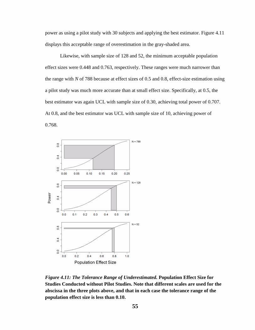
55

power as using a pilot study with 30 subjects and applying the best estimator. Figure 4.11

displays this acceptable range of overestimation in the gray-shaded area.

Likewise, with sample size of 128 and 52, the minimum acceptable population

effect sizes were 0.448 and 0.763, respectively. These ranges were much narrower than

the range with N of 788 because at effect sizes of 0.5 and 0.8, effect-size estimation using

a pilot study was much more accurate than at small effect size. Specifically, at 0.5, the

best estimator was again UCL with sample size of 0.30, achieving total power of 0.707.

At 0.8, and the best estimator was UCL with sample size of 10, achieving power of

0.768.

Figure 4.11: The Tolerance Range of Underestimated. Population Effect Size for

Studies Conducted without Pilot Studies. Note that different scales are used for the

abscissa in the three plots above, and that in each case the tolerance range of the

population effect size is less than 0.10.

56

Figure 4.12 summarizes the power, expected wasted resources, and cost per

percentage point as a function of sample size (52, 128, and 788) and population effect

size (0.2, 0.5, 0.8). In terms of power, if a researcher predicted a large effect size but an

actual effect size turned out to be 0.5 or 0.2, the power of his study was only 0.424 and

0.105, respectively. On the other extreme, if a researcher planned a sample size for

detecting a small effect and the actual population effect size turned out to be 0.5 or 0.8,

he would achieve power of 1, but would waste many of his subjects to overpower the

study.

Figure 4.12 b&c depict the relationship between the economic measures and

population effect size and sample size. On one extreme, with a sample size of 788, a

researcher would be wasting nearly $16,000 per study even if he correctly planned his

study to achieve desired power of 0.8 to detect a small population effect. This may appear

surprising since he planned his study correctly. Yet keep it in mind that his β is still 0.2,

which means that he would fail to reject a null hypothesis once every five replications,

thereby wasting 788*100*0.2 = $15,760 per study. Because detecting a small population

effect already requires a huge sample size, to minimize expected wasted resources the

desired power may have to reach a 0.90 or even a 0.95 level. On the other hand, with this

sample size of 788 and a population effect that turned out to be bigger than 0.2, expected

wasted resources becomes 0 because such a study would achieve power of 1 (i.e., β of 0).

The other extreme would be a very underpowered study. When a study was

designed to detect large effect size (i.e., sample size of 52), even when the true

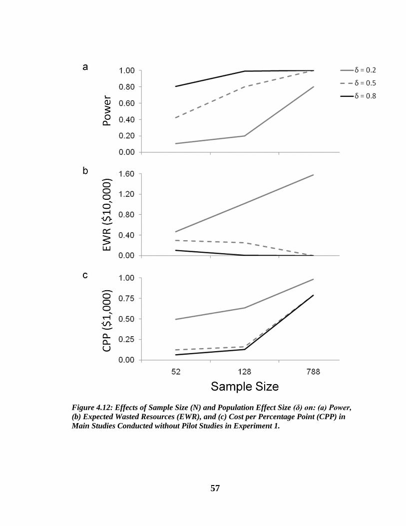
57

Figure 4.12: Effects of Sample Size (N) and Population Effect Size (δ) on: (a) Power,

(b) Expected Wasted Resources (EWR), and (c) Cost per Percentage Point (CPP) in

Main Studies Conducted without Pilot Studies in Experiment 1.

58

population effect size turned out to be small its expected wasted resources were relatively

small, approximately $5,000. Because the total study cost of the small study is relatively

inexpensive ($52,000), even though it has minimal power for detecting a small effect

(0.105). As a result, expected wasted resources were relatively low.

In terms of cost per percentage point, again a large study with sample size of 788

designed to detect a small effect was the most expensive (CPP = $985). Interestingly, a

small study with 52 subjects that attempts to detect a small effect is much more cost

efficient (CPP = 0.495). This is because, while increasing sample size from 52 to 788

increased the cost by a factor of 15 (788/52), the corresponding increase in power was

less than 8 fold (0.80/0.105).

With this CPP measure, the inefficiency of overpowered studies was also

demonstrated. For example, in detecting a population effect size of 0.5, the cost per

percentage point for a study with 52 subjects was $123, and with 128 subjects it was

$160. Again in terms of cost, smaller, underpowered studies were more efficient than

larger studies, even though the latter achieved the correct power. On the other hand,

detecting the same effect size with 788 subjects leads to CPP of $788, a nearly 400%

increase.

Null effect size. To examine whether different methods of estimating population

effect size would affect Type I error, resulting powers based on valid power and total

power at the population effect size of 0 were summarized in Table 4.5. In terms of valid

power, Type I error rates were quite well controlled, regardless of the estimation

methods, the size of error variance, and the proportion of variance removed (range =

0.043 ~ 0.055). On the other hand, Type I error rates were lower than the nominal 0.05

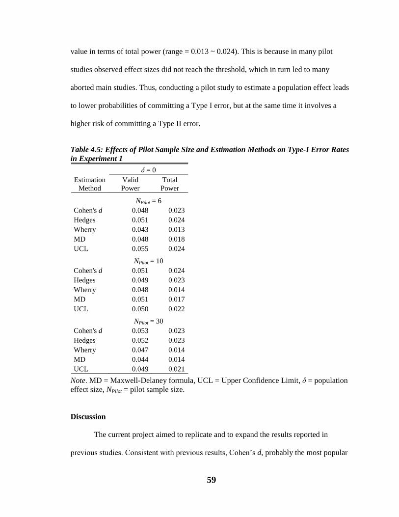
59

value in terms of total power (range = 0.013 ~ 0.024). This is because in many pilot

studies observed effect sizes did not reach the threshold, which in turn led to many

aborted main studies. Thus, conducting a pilot study to estimate a population effect leads

to lower probabilities of committing a Type I error, but at the same time it involves a

higher risk of committing a Type II error.

Table 4.5: Effects of Pilot Sample Size and Estimation Methods on Type-I Error Rates

in Experiment 1

Note. MD = Maxwell-Delaney formula, UCL = Upper Confidence Limit, δ = population

effect size, NPilot = pilot sample size.

Discussion

The current project aimed to replicate and to expand the results reported in

previous studies. Consistent with previous results, Cohen’s d, probably the most popular

Estimation

Method

δ = 0

Valid

Power

Total

Power

NPilot = 6

Cohen's d 0.048 0.023

Hedges 0.051 0.024

Wherry 0.043 0.013

MD 0.048 0.018

UCL 0.055 0.024

NPilot = 10

Cohen's d 0.051 0.024

Hedges 0.049 0.023

Wherry 0.048 0.014

MD 0.051 0.017

UCL 0.050 0.022

NPilot = 30

Cohen's d 0.053 0.023

Hedges 0.052 0.023

Wherry 0.047 0.014

MD 0.044 0.014

UCL 0.049 0.021

60

effect size measure, was a positively biased estimator of its population counterpart, and

its estimation was the least precise of the all estimation methods examined (i.e., it had the

largest standard deviations and interquartile ranges). Applying the Hedges’ formula

improved the mean bias, but this formula was negatively biased at the median. The UCL

formula was an even more negatively biased estimator then the Hedges’ formula. Its

magnitude of bias is understandable since its purpose is to ensure that a main study will

have adequate power by overestimating the standard deviation (Browne, 1995). Applying

these three formulae led to fewer aborted studies than the Wherry and MD formula. Still,

at the small population effect size of 0.2, 35~45% of the main studies were aborted.

The Wherry and MD formulae often overcorrected observed effect sizes,

converting them to 0. As a result, these formule produced very skewed, asymmetrical

distributions of observed effect size. Applying these formulae led to aborting more

studies than applying the other formulae, especially at a small effect size.

Perhaps the most important finding in this experiment is that the resulting power

was far below the desired power of 0.8, especially at the small population effect size:

power deviations ranged from -0.45 to -0.75. These degrees of power deviations were

surprising because pilot studies were designed to estimate the population effect size to

achieve the desired power over many replications, even though some of the estimators

were more biased than the others. Why was the resulting power so small?

The distribution of Cohen’s d is portrayed in Figure 4.13 to explain why this was

the case. To simplify, its distribution is assumed to be normal (Hedges & Olkin, 1985),

even though its empirical distribution could be skewed and/or leptokurtic, because of

outliers. According to the formulae (1) and (10), at the population effect size (δ) of 0.2

61

and with the pilot sample size of 6, the mean of the sampling distribution of Cohen’s d

(μd) is 0.25 with the standard deviation (σd) of 1.16.

Figure 4.13: Different proportions of the theoretical distribution of Cohen’s d at the

population effect size (δ) of 0.2. Pilot sample size is 6. The lighter gray area indicates

the proportion of the main studies aborted [i.e., p(Aborted) = p(d < dThreshold) = 0.43].

The darker gray area indicates p(Underpowered) = p(d > δ) = 0.52. The white area

indicates p(Overpowered) = p(δ ≥ d ≥ dThreshold) = 0.05.

Four things are noteworthy. First, because Cohen’s d is positively biased (i.e., μd –

δ = 0.05), the probability of the main study being underpowered is greater than 0.5: in

this case, 0.52. That is, more than half of the main studies over many replications will

have power smaller than 0.80. The darker gray area in the figure corresponds to this

probability p(Underpowered) = p(d > δ) = 0.52. Second, with the pilot sample size of 6,

the standard deviation is 1.16, far larger than the value of the population effect size. As a

result, a substantial portion of the distribution will be below the threshold value (dThreshold)

of 0.05. The lighter gray area in Figure 4.13 indicates this probability, p(Aborted) = p(d <

dThreshold) = 0.43. In other words, 43% of the main studies will be aborted because the

62

observed effect size is deemed too small or even negative. Third, the probability of d

estimated between 0.05 and 0.20 is only 1 – 0.52 – 0.43 = 0.05. That is, the probability of

the main study having the desired power of 0.80 or greater is only 5% (i.e.,

p(Overpowered) = p(δ ≥ d ≥ dThreshold) = 0.05). Of 57% of all main studies ever

conducted, 91% (i.e., 0.52/0. 57) will be underpowered, while the rest, only 9% of the

main studies, will be overpowered. Thus, positive bias and imprecise estimation, inherent

in small sample size, led to a large proportion of aborted and underpowered studies. As a

result, the resulting power described in the Results section was far below the desired level

of power. Finally, Figure 4.13 implies that the imprecision of effect-size estimation based

on a small pilot study may lead researchers to extremely erroneous conclusions. For

instance, fully 88% of this sampling distribution of Cohen’s d deviates from the

population value by more than 100% (i.e., (d < 0.0) or (0.4 < d)), and 77% deviates by

more than 200% (i.e., (d < -0.2) or (0.6 < d)). Thus, even though the true effect size is

0.2, researchers may often be led to believe that the estimated effect size would be larger

than a medium effect, and they may often be led to believe that the effect was either

practically null or a small effect in the opposite direction. This is an extreme example, but

researchers need to be aware of the very poor precision of estimation of effects based on

a small pilot study (Kraemer et al., 2006).

Applying the other methods changed these probabilities. The Hedges’ or UCL

formula alleviated this negative power deviation somewhat because these formulae

shifted the mean to the population value. In the case of the UCL, its mean was even

smaller than the population value. By doing so, they decreased the probability of main

studies being underpowered and increased the probability of main studies being

63

overpowered. As a result, the resulting power based on these methods was higher than the

power based on Cohen’s d. Even though the Hedges’ and UCL formulae had much

smaller mean observed effect size than Cohen’s d, their probabilities of aborted studies

were not substantially greater than that of Cohen’s d (see Figure 4.6). This is because

these two formulae also reduced the size of the standard deviation (see Table 4.1),

making the distribution narrower. On the other hand, applying the Wherry and MD

formulae resulted in greater power deviations than Cohen’s d. This is because these

formulae converted observed effect sizes to 0 in up to 70% of the pilot studies, which in

turn led to many aborted studies. These results suggest that if one’s purpose of

conducting a pilot study is to estimate effect size in such a way as to maximize the power

of one’s study, one’s best choice would be the UCL method.

Both measures of economic performance demonstrated the cost inefficiency of

large studies, especially if they were overpowered. This is mainly because, even though

statistical power and sample size are positively correlated, they do not increase at the

same rate. If the purpose of a study is to maximize the tradeoff between the amount of

information obtained in a study and its cost, then small, low-powered studies appeared to

be more efficient than large, high-powered studies. These results are consistent with the

notion that the goal of a study should be to maximize the ratio of the study’s scientific

value of information to the study’s total cost, instead of power (Bacchetti, 2010).

64

Chapter 5

Experiment 2

Method

Experiment 2 examined the effect of conducting pilot studies based on the

assumption that pilot studies improve the quality of the actual study (See Figures 5.1 &

5.2). This potential benefit of pilot studies will be examined by introducing two new

factors: (1) σ2

E and (2) reduction in σ2

E as a result of conducting pilot studies. In the pilot

condition, the number of cells will be 108 = 4 (Population Effect Size δ: 0, 0.2, 0.5, 0.8) x

3 (Pilot-Study Sample Size Npilot: 6, 10, 30) x 3 (Size of σ2

E: 56%, 125%, 300% of σ2

T) x

3 (Size of Reduction in σ2

E: 0%, 50%, 100%), in each of which 10,000 simulations were

run. In the non-pilot condition, the number of cells will be 36 = 4 (Population Effect Size

δ: 0, 0.2, 0.5, 0.8) x 3 (Required Sample Size for Detecting Effect Size of 0.2, 0.5, 0.8:

788, 128, 52) x 3 (Size of σ2

E: 25%, 50%, 100% of σ2

T). Thus, a total of 108+36 = 144

cells were produced.

In this experiment only Cohen’s d estimator was used because Cohen’s d, with its

positive bias, could be counteracting the attenuation of effect size caused by the error

variance. In addition, the number of cells in the pilot condition was already much larger

than Experiment 1 (108 vs. 36). If all the five estimation methods were examined, the

number of cells would have been 540. Also, the 95% confidence interval was excluded

from Experiment 2 because its width is primarily a function of sample size. For instance,

decreasing the population effect size from 0.5 to 0.2 with the sample size of 10 narrows

the width of the 95% confidence interval from 1.78 to 1.76, a small change of only 1.4%.

65

Figure 5.1: Procedural Steps for Experiment 2 Pilot Condition. (1) A value of σ

2E was

added to σ2T , increasing σ

2T by 56%, 125%, or 300%. As a result, population effect

size δ0 was attenuated by 20%, 33%, or 50% from δ. (2) An observed effect size for

the pilot study (d) was drawn from the distribution of possible values around the

true value of δ0. (3) Based on this value of d, the sample size required to achieve the

desired power of 0.8 was calculated ( ). (4) After conducting the pilot study, σ2

E was

assumed to be reduced by X (0%, 50%, or 100%), resulting in disattenuated

population effect size δ1. (5) Sample data were drawn from the distribution of

possible values around the true value of μ1, μ2, and

, and a t test was

performed. Circles indicate independent variables and squares indicate random

variables. (1) – (5) were repeated 10,000 times, and the number of p values smaller

than 0.05 were counted and divided by 10,000 to derive the observed power. Circles

indicate independent variables and squares indicate random variables.

66

Figure 5.2: Procedural Steps for Experiment 2 Non-Pilot Condition. (1) A value of σ

2E

was added to σ2T , increasing σ

2T by 56%, 125%, or 300%. As a result, population

effect size δ0 was attenuated by 20%, 33%, or 50% from δ. (2) Based on the

intuitively estimated value of δ, N is determined (i.e., 788, 128, or 52). Unlike

above, this was not a random variable. (3) Resulting power of the main study was

computed based on the combinations of δ, levels, sizes of σ2E, and N. Circles indicate

independent variables and squares indicate random variables.

On the other hand, increasing the sample size from 10 to 30 at the population effect size

of 0.5 narrows the width from 1.78 to 1.03, a reduction of over 40%.

In Experiment 2, the following independent variables were added to model the

potential procedural advantages of implementing a pilot study before its corresponding

main study. This part of the current project is predicated on the potential importance in

actual research of two additional factors not considered in Experiment 1. First, random

errors were introduced to inflate the true variance, thereby attenuating population effect

size. In this project, errors are broadly defined as any random variations caused by

different sources at any given point of data measurement, handling, and analysis. Hunter,

Schmidt, and their colleagues (e.g., Schmidt & Hunter, 1996; Schmidt & Hunter, 1999;

Schmidt, Le, & Ilies, 2003) list four major types of measurement errors: transient,

67

random-response, specific-factor, and rater-bias errors. In addition, Viswanathan (2005)

categorizes method-related sources of errors into item content, response format, and

administration.

The second factor incorporated into Experiment 2 is based on the recognition that

conducting a pilot study often allows researchers to improve the way the subsequent main

study is carried out. This point is emphasized by Kraemer and colleagues (2006) who

state:

Pilot studies are important in the preparation of proposals for hypothesis-testing

studies. They serve to check on the availability of eligible and willing subjects

using the recruitment methods proposed, to test the feasibility of the treatment and

measurement protocols, to train researchers in study tasks, and to set up data

collection, checking, storage, and retrieval capabilities. Glitches in the research

design are often found and corrected during pilot testing, leading to a better-

designed main study. (p. 489)

In other words, only by conducting pilot studies can researchers potentially find

“glitches” (different sources of random, procedural errors), correct them (eliminate or

reduce errors), and qualitatively as well as quantitatively improve the main study. One

such improvement may be reducing measurement error variance by training raters to

achieve more consistent rating (e.g., Muller & Wetzel, 1998. For other examples, see

below). The two additional independent variables in Study 2 serve to model this aspect of

pilot studies’ potential benefits.

Size of population error variance. The first independent variable unique to

Study 2 is different sizes of population error variance (σ2

E: 56.25%, 125%, 300% of σ2

T)

68

to model the attenuation of population effect size. Based on the formula of attenuated

population effect size δ0 = (μ1 – μ2)/2 2

T E , the three levels of error variance would

result in attenuations of population effect size [(δ – δ0)*100] by 20%, 33%, and 50%,

respectively. These attenuations would be found in the pilot study in the pilot condition

and in the main study in the non-pilot condition. To put these values in perspective, these

sizes of attenuation could be translated into degrees of reliability: corresponding

reliability coefficients would be 0.64, 0.44, and 0.25 (Williams & Zimmerman, 1989).

The score reliability of 0.64, only slightly below the conventional accepted level, could

introduce error variance larger than half of the true population variance. Reliabilities

ranging from 0.4 to 0.5 are said to be common among scores collected with locally

developed instruments (Kraemer, 1991), could introduce error variance 125% as large as

the true variance, thereby attenuating effect size by 33%. Finally, an single-item

instrument could result in reliability as low as 0.25 (Schmidt & Hunter, 1996),

attenuating the population effect size by more than 50%. Thus, these levels of error

variance, though seemingly high, may well creep into empirical research.

Keep in mind that, even if one achieves high score reliability in some aspects of

measurement, one’s score reliability in other aspects may well be low. For example, in

terms of Schmidt and Hunter’s conceptualization, Cronbach’s coefficient α – the most

commonly used measure of reliability in social sciences (Hogan, Benjamin, & Brezinski,

2000; Raykov & Shrout, 2002) – measures only specific-factor and random-response

errors, but not transient errors, or rater-bias errors if multiple raters are used (Schmidt &

Hunter, 1999; Schmidt et al., 2003). Thus, even if one achieves high Cronbach’s α of

69

0.90, one’s overall reliability might be much lower if the reliability in other aspects of

measurement were low (for such an example, see Schmidt & Hunter, 1996).

Size of reduction in the error variance. The second independent variable

introduced in Experiment 2 is the size of reduction in the error variance (0%, 50%, 100%

of σ2

E removed). This variable represents consequences of applying different means to

reduce error variance, as described previously.

One hundred percent removal of error variance represents the maximum possible

advantage of conducting pilot studies, whereas 0% removal represents no advantage.

Fifty percent removal represents an in-between value. Specifically, if the true variance

were inflated by 56%, 125%, and 300% but 50% of this inflation were removed, it would

result in 11%, 20%, and 33% attenuation, respectively (instead of 20%, 33%, and 50%

without disattenuation). The corresponding reliability coefficients would be 0.79, 0.64,

and 0.44. A 50% reduction in error variance can be achieved, for example, by doubling

the length of a survey instrument or the number of raters used, according to the

Spearman-Brown formula (Maxwell et al., 1991; Williams & Zimmerman, 1989).

The purpose of Experiment 2 is summarized here. Typical simulation studies

investigating effect-size estimation or power analysis assume perfect reliability (i.e., σE =

0). This is unrealistic because no measurement is perfect; there always are known or

unknown sources of variance (Hunter & Schmidt, 2004; Schmidt & Hunter, 1996;

Viswanathan, 2005). This project attempted to examine this aspect – often overlooked in

simulation studies – of effect-size estimation with pilot studies by varying the size of

error variance. Another often overlooked aspect of actual research in simulated pilot

studies is the qualitative benefits resulting from conducting small pilot studies in

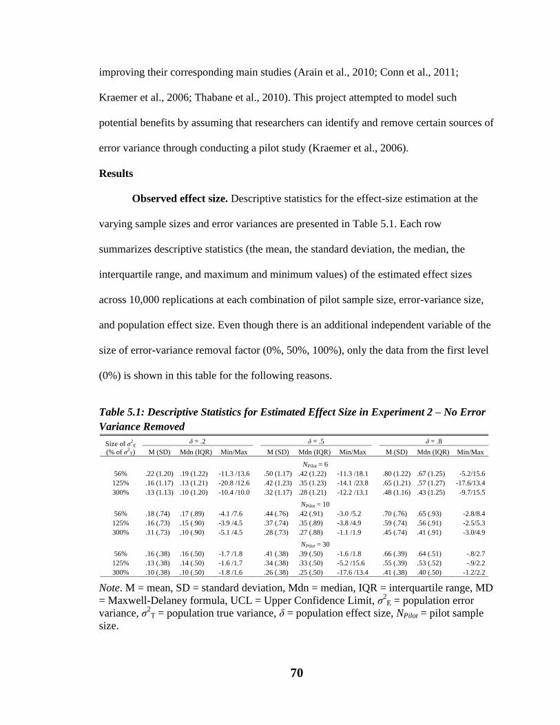
70

improving their corresponding main studies (Arain et al., 2010; Conn et al., 2011;

Kraemer et al., 2006; Thabane et al., 2010). This project attempted to model such

potential benefits by assuming that researchers can identify and remove certain sources of

error variance through conducting a pilot study (Kraemer et al., 2006).

Results

Observed effect size. Descriptive statistics for the effect-size estimation at the

varying sample sizes and error variances are presented in Table 5.1. Each row

summarizes descriptive statistics (the mean, the standard deviation, the median, the

interquartile range, and maximum and minimum values) of the estimated effect sizes

across 10,000 replications at each combination of pilot sample size, error-variance size,

and population effect size. Even though there is an additional independent variable of the

size of error-variance removal factor (0%, 50%, 100%), only the data from the first level

(0%) is shown in this table for the following reasons.

Table 5.1: Descriptive Statistics for Estimated Effect Size in Experiment 2 – No Error

Variance Removed


= Maxwell-Delaney formula, UCL = Upper Confidence Limit, σ2

E = population error

variance, σ2

T = population true variance, δ = population effect size, NPilot = pilot sample

size.

Size of σ2

E

(% of σ2

T)

δ = .2 δ = .5 δ = .8


NPilot = 6

56% .22 (1.20) .19 (1.22) -11.3 /13.6

.50 (1.17) .42 (1.22) -11.3 /18.1

.80 (1.22) .67 (1.25) -5.2/15.6

125% .16 (1.17) .13 (1.21) -20.8 /12.6

.42 (1.23) .35 (1.23) -14.1 /23.8

.65 (1.21) .57 (1.27) -17.6/13.4

300% .13 (1.13) .10 (1.20) -10.4 /10.0

.32 (1.17) .28 (1.21) -12.2 /13.1

.48 (1.16) .43 (1.25) -9.7/15.5

NPilot = 10

56% .18 (.74) .17 (.89) -4.1 /7.6

.44 (.76) .42 (.91) -3.0 /5.2

.70 (.76) .65 (.93) -2.8/8.4

125% .16 (.73) .15 (.90) -3.9 /4.5

.37 (.74) .35 (.89) -3.8 /4.9

.59 (.74) .56 (.91) -2.5/5.3

300% .11 (.73) .10 (.90) -5.1 /4.5

.28 (.73) .27 (.88) -1.1 /1.9

.45 (.74) .41 (.91) -3.0/4.9

NPilot = 30

56% .16 (.38) .16 (.50) -1.7 /1.8

.41 (.38) .39 (.50) -1.6 /1.8

.66 (.39) .64 (.51) -.8/2.7

125% .13 (.38) .14 (.50) -1.6 /1.7

.34 (.38) .33 (.50) -5.2 /15.6

.55 (.39) .53 (.52) -.9/2.2

300% .10 (.38) .10 (.50) -1.8 /1.6 .26 (.38) .25 (.50) -17.6 /13.4 .41 (.38) .40 (.50) -1.2/2.2

71

First, this error-variance removal variable affects only the results in the main

study, not in the pilot study, so theoretically the results across the three levels within this

variable should not havehad any impact on the estimate derived from the pilot study.

Second, the results were in fact very similar across the three levels within this variable:

the descriptive statistics for the observed effect sizes were all within a range of 0.01 from

each other. Thus, this section focuses on the results from the first level of 0% error

reduction, unless the results from the main studies are being described.

Measures of accuracy of effect-size estimation. As expected, various sizes of

error variance, introduced in Experiment 2, inflated the total observed variance, thereby

attenuating the means and the medians of the observed effect sizes. In this analysis,

relative attenuation is defined as [(δ - )/δ], where is the mean or the median observed

effect size, and δ is the value of the population effect size. As noted above, with error

variances equal to 56%, 125%, and 300% of the true score variance, the population

effect size would be expected to be attenuated by 20%, 33%, and 50%, respectively.

Error variance of 56%. With a pilot sample size of six, the relative attenuation of

the mean observed effect sizes across the three levels of population effect size was -3%,

meaning that the mean of the observed effect sizes was greater than 0.2. In fact, with this

sample size, as shown in the top row of Table 5.1, the mean observed effect sizes were

0.22, 0.50, 0.80. This is because Cohen’s d is known to be a positively biased estimator

of the population effect size, and the magnitude of positive bias can be computed from

Equation x above as

Relative Positive Bias = (4df – 1)/(4df – 4) (13)

72

With a sample size of six the Relative Positive Bias would be 15/12 = 1.25, for an

inflation of 25%. Thus, this effectively canceled out the 20% attenuation resulting from

the introduction of error variance (i.e., 1.25 x 0.80 = 1.00). On the other hand, the mean

relative attenuation of the median observed effect sizes across the three levels of the

population effect size was 12%. This is because the median of Cohen’s d is a much less

biased estimator of the population effect size than its mean, and thus did not offset as

completely the introduction of error variance.

With a pilot sample size of 10, the relative attenuation of the means across the

three levels of population effect size was 12% for the means and 17% for the medians.

With a pilot sample size of 30, the relative attenuation of the means across the three

levels of population effect size was 19% for the means and 21% for the medians. Thus,

the pilot sample size and the size of attenuation were positively correlated. This is

because the magnitude of the positive bias of Cohen’s d is known to decrease as the

sample size increases. From the above formula, positive biases with pilot sample sizes of

10 and 30 are 11% and 3%, respectively. Thus, overall theoretical attenuations are 1.11 x

0.80 = 0.88, and 1.03 x 0.80 = 0.82. These values are in fact very similar to the empirical

values obtained for the mean in this experiment (i.e., .88 and .81, respectively).

Error variance of 125% and 300%. As expected, greater error variances led to

greater attenuations. With the error variance as 125% as large as the true variance, the

mean relative attenuation across nine conditions (3 Pilot Sample Sizes x 3 Population

Effect Sizes) was 25% for the means and 31% for the medians. With the error variance

300% as large as the true variance, the mean relative attenuation across nine conditions

was 43% for the means and 48% for the medians.

73

Measures of precision of effect-size estimation. To examine the effect of

introducing different sizes of error variances on the precision of effect-size estimation,

standard deviations and interquartile ranges of observed effect sizes were compared

across the three different sizes of error variances. Interestingly, as shown by entries

within parentheses in Table 5.1, the standard deviations were influenced very little by the

differing sizes of error variances. For instance, with a pilot sample size of six, the mean

standard deviations across the three population-effect-size conditions were 1.20, 1.20,

and 1.15 with 56%, 125%, and 300% error variances, respectively. The mean

interquartile ranges were 1.23, 1.24, and 1.22. With a pilot sample size of 10, the range of

the comparable mean standard deviations was only from 0.73 to 0.75, and the range of

the mean interquartile ranges was only from 0.90 to 0.91. With a pilot sample size of 30,

the mean standard deviations were all 0.38 to 2 significant digits, and the mean

interquartile range ranged just from 0.50 to 0.51. Thus, the sample-size variable had a

much greater effect on the size of the variability measures than the size of error variance.

This is explained by Formula 1: according to this formula, increasing a population effect

size from 0.2 to 0.5 based on the sample size of 10 will increase the standard deviation of

Cohen’s d from 0.73 to 0.74, only by 0.01 point. On the other hand, increasing the sample

size from 10 to 30 at the population effect size of 0.2 will decrease the standard deviation

from 0.73 to 0.38. That is, introducing error variance into the population variance will

inflate the observed variance and attenuate the effect size, but will hardly affect the

precision of effect-size estimation.

Estimated required sample size. Based on the observed effect sizes obtained

initially, estimated required sample sizes ( ) for achieving power of 0.8 at α = 0.05 were

74

calculated. As in Experiment 1, the threshold of the observed effect size (dThreshold) was

set to 0.05. That is, any observed effect size in a pilot study smaller than 0.05 was

deemed too small, which in turn led to an aborted main study. Also, five percentile points

(10th

, 25th

, 50th

, 75th

, and 90th

) were computed instead of the mean/median and the

standard deviation/interquartile range.

Table 5.2: Quantiles of the Distribution of Estimated Required Sample Size ( ) in

Experiment 2 – No Error Variance Removed

Note. NA indicates that the main study was aborted because of too small or negative

observed effect size (d < 0.05), σ2

E = population error variance, σ2

T = population true

variance, δ = population effect size, NPilot = pilot sample size.

Table 5.2 presents the five percentile points of estimated required sample sizes at

each level of the three error-variance sizes and three population effect sizes along with

the correct sample sizes to achieve power of 0.8. First, notice that many cells had NA’s in

the table, and that the prevalence of the NA’s in each row is a function of the error-

variance size. For instance, with 56% error variance and a pilot sample size of 30, an NA

appeared at both the 10th

and 25th

percentiles at a population effect size of 0.2, appeared

at only the 10th

percentile at a population effect size of 0.5, but did not appear at any

percentile for a population effect size of 0.8. On the other hand, with 300% error

variance and a pilot size of 30, an NA appeared at the 25th

percentile at the population

Size of σ2

E

(% of σ2

T)

δ = .2 (N = 788) δ = .5 (N = 128) δ = .8 (N = 52)

10 / 25 / 50 / 75 / 90 10 / 25 / 50 / 75 / 90 10 / 25 / 50 / 75 / 90

NPilot = 6

56% NA / NA / 12 / 82 / 420

NA / NA / 20 / 88 / 426

NA / 6 / 22 / 82 / 328

125% NA / NA / 10 / 84 / 438

NA / NA / 18 / 88 / 446

NA / NA / 20 / 78.5 / 376

300% NA / NA / 8 / 76 / 454

NA / NA / 14 / 86 / 410

NA / NA / 20 / 84 / 410

NPilot = 10

56% NA / NA / 24 / 148 / 708

NA / NA / 36 / 134 / 582

NA / 12 / 36 / 114 / 428

125% NA / NA / 24 / 142 / 714

NA / NA / 36 / 138 / 608

NA / 10 / 38 / 126 / 522

300% NA / NA / 18 / 130 / 746

NA / NA / 34 / 150 / 708

NA / NA / 36 / 138 / 620

NPilot = 30

56% NA / NA / 90 / 406 / 1567

NA / 38 / 104 / 312 / 1086

20 / 36 / 68 / 156 / 464

125% NA / NA / 80 / 390 / 1490

NA / 30 / 106 / 350 / 1276

12 / 38 / 82 / 208 / 678

300% NA / NA / 62 / 372 / 1446

NA / NA / 102 / 364 / 1432

NA / 40 / 100 / 302 / 970

75

effect sizes of 0.2 and 0.5, and at the 10th

percentile at the population effect size of 0.8.

This is understandable because, while the median observed effect size was on average

attenuated by 20% with the error variance of 56% (Table 5.1), the size of attenuation was

50% with the variance of 300%. Thus, greater error variance, resulting in greater

attenuation, also led to more aborted main studies.

In terms of estimated required sample size, Cohen’s d tended either to lead to

abandonment of the main study or to an underestimation of the required sample size or

led to abandonment of the main study, similar to the results in Experiment 1. This

underestimation of N by Cohen’s d appeared to have been moderated by the independent

variables. For instance, at the population effect size of 0.2, Cohen’s d underestimated the

required sample size in more than 90% of the simulated pilot studies with the pilot

sample sizes of six and 10, and in more than 75% of the studies with the pilot sample size

of 30. At this effect size the degree of underestimation did not differ across levels of the

error-variance size. As the population effect size increased, Cohen’s d started

overestimating the required sample size, at least at the 75th

and 90th

percentiles of the

distribution of N̂ for Npilot of 6 or 10, and also at the 50th

percentile and above for Npilot of

30, and the degree of overestimation was positively correlated with the size of the error

variance. For instance, with the 56% variance and with pilot sample size of 30, the

median required sample size at a population effect size of 0.8 was overestimated as 68 by

Cohen’s d, but with the 300% variance the median required sample size was 100.

Probability of the main study being aborted. Similar to Experiment 1, many

pilot studies yielded an estimated effect size below the threshold of 0.05; as a result,

instances of aborted main studies were likewise pervasive. To quantify the proportion of

76

aborted main studies to all simulated studies, the instances of aborted studies were

counted and divided by the number of replications (10,000). Results are summarized in

Figure 5.3.

Figure 5.3: Probability of the Main Study Being Aborted Based on Pilot Results in

Experiment 2.

The figure suggests that the independent variables interact to influence the

probability of main studies being aborted. At a population effect size of 0.2, the error-

variance size had little effect on the probability: regardless of the variance size, the

77

probability hovered around 40%. At larger population effect sizes, the variance size had

larger effects, but not as large as the effects of the pilot sample size on the probability of

aborting the study. For instance, increasing the error variance from 52% to 300% resulted

in an approximately 9 percentage-point increase in the probability of the main studies

being aborted at the population effect size of 0.5, and an 11 percentage-point increase at

the effect size of 0.8. In contrast, increasing the pilot sample size from six to 30 resulted

in a reduction of the probability by around 13 and 17 percentage points at the medium

and large effect sizes, respectively. While the three independent variables interacted to

influence the probability, the population effect size and pilot sample size had a greater

influence than the error-variance size.

Power deviation. As in Experiment 1, some main studies were aborted because

the observed effect sizes did not reach the threshold value in their pilot-study

counterparts, which complicated power analysis. To deal with this problem, two types of

power, total power and valid power, were again computed. After these powers had been

computed within each condition, power deviations were calculated by subtracting the

desired level of power of 0.8 from both powers. The value of 0 indicates that the resulting

power matched the desired power, while positive and negative values indicate

overpowering and underpowering, respectively. Figures 5.4 and 5.5 summarize the result

of power deviations based on total power and valid power.

Power deviation - total power. Similar to the Experiment 1 results, underpowered

studies were pervasive, indicated by many downward lines. Recall that this is in large

part because most of the studies that would have been overpowered were aborted and

78

thus combined with those studies that were underpowered and actually carried out. In

fact there was no single condition that resulted in overpowering. Also similar to

Figure 5.4: Power Deviation Based on Total Power in Experiment 2.

Figure 5.5: Power Deviation Based on Valid Power in Experiment 2.

79

Experiment 1, the most influential factor apparently was the size of the population effect. For

instance, at the small effect size power deviations were up to -70 percentage points, while at the

large effect size deviations were up to -50 percentage points. The pilot sample size was also an

influential factor, especially at larger effect sizes: within each panel an increase in pilot sample

size was accompanied by a decrease in a negative power deviation, and this reduction was

greater at medium and large effect sizes.

The error-variance size, though not as influential as the two factors described above, did

affect power deviations, especially at larger effect sizes. When no error variance was removed,

increasing the error-variance size led to greater negative power deviations by five to 20

percentage points, and its effect was particularly large at medium and large population effect

sizes and with the pilot sample size of 30. At the population effect size of 0.2, the effect of the

variance size was less pronounced with any of the pilot sample sizes.

Removing part or all of the error variance understandably improved resulting power.

Overall, greater removal led to greater improvement. The magnitude of this improvement

depended on all the other factors. First, the magnitude of improvement was positively associated

with the population effect size. While removing all of the error variance reduced negative power

deviations by up to 10 percentage points compared to the no-removal condition when the

population effect size was small, this reduction was up to 30 percentage points when the

population effect size was large. Second, larger error-variance sizes and pilot sample sizes were

associated with greater improvement. For instance, at the population effect size of 0.8, greater

improvements occurred with the pilot sample size of 30 and the error variance of 300% than any

80

other conditions. These results indicate that researchers may benefit from conducting pilot

studies if they expect a medium to large population effect, employ a pilot sample size of around

30, and suspect a moderate to large error variance which might subsequently be reduced based

on the experience gained in the pilot study.

Power deviation - valid power. Figure 5.5 summarizes the results of power analysis

based on valid pilot studies and resulting power deviations. Overall patterns were similar to the

patterns based on total power deviations, with all deviations shifted upward. The mean power

deviation of all 81 conditions was -0.43 for total power deviations and -0.29 for valid power

deviations. Yet, all estimation methods displayed considerable underpowering at a population

effect size of 0.2 regardless of the levels of the other variables (the mean valid power deviations

across the 27 conditions was -0.49 at the population effect size of 0.2).

Measures of economic performance. To compute the economic efficiency of

conducting pilot studies, expected wasted resources and cost per percentage point were

computed in the same way as in Experiment 1. Tables 5.3 and 5.4 summarize how the

independent variables interacted to influence expected wasted resources and cost per percentage

point, respectively.

In term of expected wasted resources, four things are noteworthy. First, as the pilot

sample size increased from six to 30, expected wasted resources also increased, which is

consistent with the results from Experiment 1. Again, this positive relationship between pilot

sample sizes and expected wasted resources makes sense because the improvement in power was

not as rapid as the increase in the total study cost. Second, as

Table 5.3: Expected Wasted Resources in Experiment 2

81

Note. Expected Wasted Resources = ([Median Total Study Cost] * [1 – Total Power]), σ

2E =

population error variance, σ2

T = population true variance, δ = population effect size, NPilot = pilot

sample size.

Table 5.4: Cost per Percentage Point in Experiment 2

Note. Cost per Percentage Point = ([Median Total Study Cost] / [Total Power * 100]), σ

2E =

population error variance, σ2

T = population true variance, δ = population effect size, NPilot = pilot

sample size.

the population effect size increased from 0.2 to 0.8, overall expected wasted resources decreased,

particularly with larger pilot sample sizes. This is because, at a large effect size, fewer subjects

were required to achieve high power than at smaller effect sizes.

Third, as the error variance increased from 56% to 300% of the population true variance,

the rate of change in expected wasted resources depended on the population effect size. For

Size of σ2

E

(% of σ2

T)

δ = .2 δ = .5 δ = .8

σ2

E Removed 0% 50% 100%

0% 50% 100%

0% 50% 100%

NPilot = 6

56%

$ 1,577 $ 1,551 $ 1,513

$ 1,851 $ 1,792 $ 1,709

$ 1,631 $ 1,542 $ 1,452

125%

$ 1,426 $ 1,393 $ 1,350

$ 1,814 $ 1,739 $ 1,601

$ 1,664 $ 1,644 $ 1,472

300%

$ 1,286 $ 1,432 $ 1,352

$ 1,627 $ 1,658 $ 1,491

$ 1,874 $ 1,563 $ 1,319

NPilot = 10

56%

$ 2,856 $ 2,641 $ 2,573

$ 2,978 $ 2,823 $ 2,681

$ 2,277 $ 2,087 $ 1,895

125%

$ 2,936 $ 2,697 $ 2,583

$ 3,188 $ 2,837 $ 2,596

$ 2,666 $ 2,361 $ 2,025

300%

$ 2,513 $ 2,422 $ 2,272

$ 3,327 $ 2,791 $ 2,475

$ 2,950 $ 2,583 $ 2,070

NPilot = 30

56%

$ 8,974 $ 8,821 $ 8,166

$ 6,183 $ 5,695 $ 5,059

$ 3,092 $ 2,644 $ 2,077

125%

$ 8,749 $ 8,852 $ 7,778

$ 7,256 $ 6,296 $ 5,411

$ 4,243 $ 3,321 $ 2,318

300% $ 7,820 $ 7,040 $ 7,020 $ 8,340 $ 7,263 $ 5,771 $ 6,160 $ 4,666 $ 3,219

Size of σ2

E

(% of σ2

T)

δ = .2 δ = .5 δ = .8

σ2

E Removed 0% 50% 100% 0% 50% 100% 0% 50% 100%

NPilot = 6

56%

$ 145 $ 130 $ 113

$ 90 $ 84 $ 76

$ 67 $ 62 $ 58

125%

$ 148 $ 124 $ 103

$ 98 $ 87 $ 72

$ 72 $ 68 $ 59

300%

$ 172 $ 153 $ 103

$ 107 $ 89 $ 68

$ 93 $ 69 $ 53

NPilot = 10

56%

$ 213 $ 183 $ 163

$ 130 $ 119 $ 110

$ 91 $ 84 $ 78

125%

$ 249 $ 204 $ 166

$ 150 $ 124 $ 107

$ 108 $ 94 $ 83

300%

$ 273 $ 207 $ 149

$ 180 $ 132 $ 102

$ 128 $ 105 $ 84

NPilot = 30

56%

$ 476 $ 453 $ 392

$ 249 $ 233 $ 214

$ 143 $ 134 $ 123

125%

$ 538 $ 472 $ 376

$ 292 $ 253 $ 227

$ 180 $ 161 $ 141

300% $ 614 $ 440 $ 345 $ 359 $ 293 $ 235 $ 247 $ 203 $ 175

82

example, the mean expected wasted resources across nine conditions (3 Pilot Sizes x 3 Removal

Sizes) at the small population effect size decreased from $4,297 with 56% error variance to

$3,684 with 300%, a decrease of 14%. On the other hand, the mean expected wasted resources at

the large population effect size increased from $2,077 with 56% error variance to $2,934 with

300%, an increase of 41%. At the medium population effect size, the change was a 14% increase.

It appears that a complex interplay among the factors examined contributed to this observed

pattern. Although the resulting total power decreased, as expected, regardless of the population

effect size as the error variance increased, the effect of the error variance on the total cost was

moderated by the effect size. For instance, the median total cost was negatively associated with

the error-variance size at small and medium effect sizes, but the direction was opposite at the

large effect size. This differential effect of the error variance on the cost may be at least partially

mediated by the interaction between the rate of studies being aborted and estimated required

sample sizes.

Fourth, the removal of the error variance was negatively correlated with expected wasted

resources; that is, the greater the portion of error variance removed, the greater the reduction in

expected wasted resources became. This effect of variance removal was moderated by the

population effect size. For example, the mean expected wasted resources across nine conditions

(3 Pilot Sizes x 3 Error-Variance Sizes) at the small population effect size decreased from $4,237

with no error-variance removal to $3,845 with 100% error removal, a decrease by 9%. On the

other hand, at the large effect size the mean wasted resources decreased from $2,951 to $1,983, a

33% reduction. Similarly, the effect of error-variance removal was greater when the size of the

error variance was larger. The reduction in mean expected wasted resource (across 9 conditions:

83

3 Population Effect Sizes x 3 Sample Sizes) by eliminating the error variance was 14% with the

56% error variance and 25% with the 300% variance. It is also interesting to note that expected

wasted resources displayed certain non-linear behavior. At the small population effect size with

the pilot sample size of 6, the relationship between the variance removal and the wasted

resources was an inverted U with the 300% error variance. The same pattern was observed at the

medium effect size, but not at the large effect. This may be caused by unreliability in the

computational results: with this sample size and error variance size, many studies were aborted at

medium and large effect sizes; therefore, small random variations in the results may have caused

certain erratic behaviors. At any rate, these results underscore how adding variables such as error

variance and its removal – practical yet often neglected in simulation studies – could increase the

complexity of the power analysis as well as economic performance.

Similar patterns were also found in cost per percentage point (Table 5.4). Specifically,

this variable was on average inversely related with population effect size. Also, as pilot sample

size increased, the cost increased as well. Finally, the error variance was positively correlated

with cost per percentage point (larger variance led to greater cost), while the amount of error-

variance removal was negatively associated with cost (i.e., larger removal led to smaller cost).

These results again indicate that researchers may be able to improve the economic efficiency of

their studies by conducting pilot studies when they expect a medium to large population effect

size, employ a pilot sample size of around 30, and suspect a moderate to large error variance.

Power, EWR, and CCP of studies conducted without pilot studies. The purpose of

conducting a pilot study prior to a main study is to estimate an unknown population effect size

for calculating the sample size necessary to achieve a desired level of power. Yet, the above

84

results suggest that, if a pilot study of small sample size (30 or less) was used and/or if the

population effect size of interest is small, the desired power was rarely achieved, either because

of overestimation of d or severe underestimation leading to abandonment of the main study.

Larger error variances tended to exacerbate this power deviation. While removing or eliminating

the error variance generally improved the resulting power, the improvement was modest,

especially at small to medium population effect sizes. Now researchers may be asking whether

they may be better off if they simply estimate the population effect size of interest, in the

presence of random error variance, using other means (e.g., based on their experience,

minimally-important difference, past publications, meta-analysis) because these means are

advocated by certain methodologists (e.g., Kraemer et al., 2006).

As stated in Experiment 1, researchers tend to underestimate the standard deviation of the

effect when estimating a particular population effect a priori, thereby overestimating the effect

size and underpowering their studies (Charles et al., 2009; Vickers, 2003). Yet, the results

reported above indicated that, because the effect-size estimation based on pilot studies was so

inaccurate and imprecise that researchers had considerable room for overestimation to achieve a

similar degree of power. Recall that, at the small population effect size, researchers could

underestimate the standard deviation by 57% and still achieve the same level of power as using a

pilot study of 30 participants and the best UCL estimator.

The following section attempted to answer the question: in the presence of a certain

amount of error variance, which method of estimation would be better in achieving power,

conducting a pilot study or intuitively predicting population effect size? In other words, what is

85

the acceptable degree of overestimating population effect size, assuming that conducting pilot

studies would result in a certain degree of variance removal and improvement in power?

This question was answered by taking the following steps. First, sample sizes of 788,

128, and 52 were chosen as the levels of an independent variable (the correct sample sizes to

achieve power of 0.8 at population effect sizes of 0.2, 0.5, 0.8). Second, power analysis was

performed for each combination of these sample sizes with different error-variance sizes. Then

minimally acceptable non-attenuated population effect size was computed by finding an effect

size such that one would achieve the same level of power using pilot results under a realistic

circumstance: the error variance was reduced by 50% after conducting a pilot study. For

instance, at a population effect size of 0.2 with the error variance of 56%, conducting a pilot

study with 30 participants achieved the total power of 0.265 assuming 50% removal of the error

variance. With sample size of 788 and the error variance of 56%, the minimum population effect

size to achieve the power of 0.265 is 0.119, only a little more than half the predicted population

effect size. That is, if a researcher overestimated population effect size as 0.2 and planned his

study accordingly, as long as the actual population effect size was above 0.119 (and thus

attenuated population effect size of 0.119 x 0.8 = 0.095), he would on average achieve higher

power than conducting a pilot study with 30 subjects assuming 50% removal of the error

variance. In other words, even if his predicted population standard deviation was only 60% as

large as the true population value, his study would still achieve the same degree of power as

using a pilot study with 30 subjects and assuming that 50% of the error variance would be

removed after conducting a pilot study. With error variances of 125% and 300%, such minimum

population effect sizes were 0.138 and 0.160, respectively.

86

Likewise, minimum accepted population effect sizes were computed with the samples

sizes of 128 and 52. With a sample size of 128, the minimum acceptable non-attenuated

population effect sizes with error variances of 56%, 125%, and 300% were 0.479, 0.544, and

0.661, respectively. With sample size of 52, the minimum acceptable population effect sizes

were 0.910, 1.065, and 1.313, respectively. That is, if one planned his study to detect the

population effect size of 0.5 without knowing that the error variance would be 125% as large as

the true population variance, he would not achieve the same level of power (0.530) based on a

pilot result unless the non-attenuated population effect size was actually 0.544, greater than his

predicted 0.5. These results suggest that conducting a pilot study offers no advantage when one

attempts to detect a small population effect, regardless of the size of error variance, at least as far

as the pilot sizes examined in this project are concerned. On the other hand, when detecting

medium to large population effect sizes, conducting a pilot study may offer certain advantages in

achieving desired power, especially when the error variance is large.

Table 5.5 summarizes the power, expected wasted resources, and cost per percentage

point as a function of sample sizes (52, 128, and 788), population effect sizes (0.2, 0.5, 0.8), and

error-variance sizes (52%, 125%, 300%). In terms of power, if a researcher predicted a large

effect size but the actual effect size turned out to be 0.5 or 0.2, the power of his study was only

0.29 and 0.08 with the 56% error variance, and 0.14 and 0.05 with the 300% error variance,

respectively. At the other extreme, if a researcher planned a sample size for detecting a small

effect and the actual population effect size turned out to be 0.5 or 0.8, he would achieve power of

at least 0.94 regardless of the error-variance size, but would waste many of his subjects to

overpower the study.

87

Table 5.5: Effects of Sample Size and δ on Power, Expected Wasted Resources, and Cost per

Percentage Point in Main Studies Conducted without Pilot Studies in Experiment 2

Note. EWR = Expected Wasted Resources, CPP = Cost per Percentage Point, σ

2E = population

error variance, σ2

T = population true variance, δ = population effect size, N = Sample Size.

The relationship of the economic measures with the independent variables is presented in

Table 5.5. At one extreme, with a sample size of 788, a researcher will be wasting $56,075 per

study in the long run if the error variance is 300% as large as the population variance. This is

because his β is 0.71, which means that he would fail to reject a null hypothesis three times out

of every five replications, thereby wasting 788*100*0.71 = $56,075 per study over many

replications. Because detecting a small population effect already requires a huge sample size, to

minimize expected wasted resources the desired power may have to reach a 0.90 or even a 0.95

level especially if one suspects a moderate to large error variance. On the other hand, with this

sample size of 788, if a population effect turned out to be bigger than 0.2, expected wasted

resources becomes much smaller because such a study would achieve power close to 1.

The other extreme would be a very underpowered study. When a study was designed to

detect a large effect size (i.e., sample size of 52) and when the true population effect size turned

out to be small, its expected wasted resources were relatively small, less than $5,000. This is

Size of σ2

E

(% of σ2

T)

δ = .2 δ = .5 δ = .8

Power EWR CPP Power EWR CPP Power EWR CPP

N = 52

56% 0.08 $ 4,775 $ 637

0.29 $ 3,678 $ 178

0.62 $ 1,981 $ 84

125% 0.07 $ 4,845 $ 761

0.22 $ 4,070 $ 239

0.47 $ 2,753 $ 111

300% 0.05 $ 4,919 $ 961

0.14 $ 4,467 $ 369

0.29 $ 3,678 $ 178

N = 128

56% 0.14 $ 10,955 $ 888

0.61 $ 4,962 $ 209

0.95 $ 656 $ 135

125% 0.11 $ 11,355 $ 1,134

0.46 $ 6,852 $ 275

0.85 $ 1,927 $ 151

300% 0.08 $ 11,764 $ 1,581

0.29 $ 9,102 $ 443

0.61 $ 4,962 $ 209

N = 788

56% 0.61 $ 30,621 $ 1,289

1.00 $ 10 $ 788

1.00 $ - $ 788

125% 0.46 $ 42,251 $ 1,699

1.00 $ 263 $ 791

1.00 $ - $ 788

300% 0.29 $ 56,075 $ 2,732 0.94 $ 4,824 $ 839 1.00 $ 10 $ 788

88

because the total study cost of such a small study is relatively inexpensive ($5,200), even though

it has minimal power for detecting a small effect (0.05). As a result, expected wasted resources

would be relatively low.

In terms of cost per percentage point, again a large study with sample size of 788

designed to detect a small effect was the most expensive (CPP = $1,289~$2,732). Interestingly, a

small study with 52 subjects that attempts to detect a small effect turned out to be much more

cost efficient (CPP = $637~$961). With this CPP measure, the inefficiency of overpowered

studies was also demonstrated. For example, in detecting a population effect size of 0.5, the cost

per percentage point for a study with 52 subjects ranged $178~$369, and with 128 subjects

$209~$443. Again in terms of cost, smaller, underpowered studies were more efficient than

larger studies, even though the latter achieved the correct power. On the other hand, detecting the

same effect size with 788 subjects leads to much greater costs per percentage point of

$788~$839.

Null effect size. To examine whether different methods of estimating population effect

size would affect Type I error, resulting powers based on valid power and total power at the

population effect size of 0 were summarized in Table 5.6. Similar to the results in Experiment 1,

Type I error rates were quite well controlled in terms of valid power, regardless of the estimation

methods, the size of error variance, and the proportion of variance removed (range = 0.047 ~

0.058). On the other hand, Type I error rates were lower than the nominal 0.05 value in terms of

total power (range = 0.021 ~ 0.027). This is again because in many pilot studies observed effect

sizes did not reach the threshold, which in turn led to many aborted main studies. Thus,

conducting a pilot study to estimate a population effect leads to lower probabilities of

89

committing a Type I error, but at the same time it involves a higher risk of committing a Type II

error.

Table 5.6: Effects of Pilot Sample Size, Error-Variance Size, and Proportion of Error

Variance Removed on Type-I Error Rates in Experiment 2 (10000 Replications).

Note. σ

2E = population error variance, σ

2T = population true variance, NPilot = pilot sample size

Discussion

Experiment 2 attempted to examine two aspects of effect-size estimation based on pilot

studies that are typically neglected in simulation studies: 1) introducing an error variance to

inflate the true population variance and to attenuate its corresponding population effect size; and

2) removing a portion or all of the error variance based on the assumption that running a pilot

study would allow researchers to find and correct glitches in their studies. The goal of

Experiment 2 was to model the potential procedural advantages of implementing a pilot study

before its corresponding main study was conducted.

In general, larger error variances led to greater attenuations of observed effect sizes,

greater underestimation of required sample sizes to achieve the desired level of power, and

greater negative power deviations. Larger error variances also tended to cause greater economic

Size of σ2

E

(% of σ2

T)

σ2

E Removed = 0% σ2

E Removed = 50% σ2

E Removed = 100%

Valid Power Total Power



NPilot = 6

56% 0.051 0.024

0.052 0.025

0.053 0.025

125% 0.054 0.026

0.053 0.025

0.050 0.024

300% 0.054 0.025

0.058 0.027

0.051 0.024

NPilot = 10

56% 0.052 0.025

0.054 0.025

0.052 0.024

125% 0.053 0.025

0.050 0.023

0.051 0.024

300% 0.047 0.022

0.053 0.024

0.051 0.024

NPilot = 30

56% 0.049 0.022

0.055 0.024

0.050 0.023

125% 0.053 0.023

0.053 0.023

0.053 0.024

300% 0.047 0.021 0.051 0.023 0.051 0.023

90

inefficiencies in terms of both expected wasted resources and cost per percentage point.

Interestingly these effects of the error variance were moderated by both population effect sizes

and pilot sample sizes. At smaller effect sizes, using pilot studies was a very inaccurate and

imprecise means of estimating the effect sizes. As a result, even the largest error variance (300%

as large as the true population variance) had little effect on the dependent variables examined.

Nevertheless, as the population size increased, the effects of larger error variances became much

more pronounced. Similarly, the effects of error variances were positively correlated with the

size of pilot study: bigger pilot studies that typically achieved more accurate and precise

estimation of the population effect size were more affected by larger error variances.

The greater the portions of variance removed, the smaller power deviations became.

Larger variance removal also tended to improve economic inefficiencies to a greater extent.

These improvements tended to be even larger when the population effect size, pilot sample size,

and error variance were also large. These results suggest that researchers benefit most from

conducting a pilot study when they attempt to detect a medium to large effect with a relatively

large pilot study of around 30 participants and when they suspect large error variances.

Conversely, when researchers attempt to detect small population effect sizes, conducting pilot

studies does not appear to improve the main study in terms of power and economic performance,

regardless of how large the error variance is or what portion of it is removed.

91

Chapter 6

Summary and Concluding Discussion

Objective 1

The first objective of the current project was to investigate how conducting a pilot study

of varying sample sizes, combined with various effect-size estimation methods, would affect the

accuracy and precision of effect-size and sample-size estimation, and the resulting power of the

final study being planned. For this purpose, this project compared the results of a pilot condition

with those of a non-pilot condition.

Accuracy and precision in estimating population effect sizes. Consistent with the

results reported previously (e.g., Hedges & Olkin, 1985; Roberts & Henson, 2002), Cohen’s d

was a positively biased and very imprecise estimator of its population counterpart. Applying the

Hedges’ formula improved the mean bias, but this formula was negatively biased at the median.

The UCL, Wherry, and MD formulae were also negatively biased estimators, but the Wherry and

MD formulae often overcorrected observed effect sizes, converting them to 0. Increasing the

pilot sample size from six to 30 considerably improved both the precision and accuracy of

estimation, but at an effect size of 0.2, none of the estimators had a standard deviation or an

interquartile range narrower than the value of the effect size itself, causing considerable

uncertainties in estimation.

Accuracy and precision in estimating required sample sizes and the resulting power.

Reflecting the considerable imprecision, observed effect sizes did not reach the threshold value

of 0.05 in many of the pilot studies. As a result, many of the main studies were aborted,

especially when the Wherry and MD formulae were applied, and when the effect size and pilot

92

sample size were small. In the worst case scenario, up to 70% of the main studies were aborted.

As a result, required sample sizes for main studies that had not been aborted were often

underestimated (see Figure 4.13).

In this experiment, pilot studies were designed to estimate the population effect size to

achieve the desired power over many replications. In fact, the mean (and in some cases the

median) observed effect sizes were fairly close to the population effect sizes. Nevertheless, a

surprising finding in this experiment is that, even with the pilot sample size of 30, the resulting

power deviated from the desired 0.80 level by -0.45 to -0.75 at the population effect size of 0.2,

and by -0.10 to -0.35 at the effect size of 0.5. Only at the population effect size of 0.8, the power

deviations fell within -0.05 points. These results together suggest that researchers need to be

aware of the shortcomings of conducting pilot studies to estimate population effects: namely,

their inaccuracy and imprecision, and the risk in aborting the main studies. If the pilot sample

sizes were too small compared to the needed sample size, and if an inappropriate correction

method were applied, conducting pilot studies can grossly overestimate required sample sizes,

and thus the resulting power of the main studies could be far from the desired level.

Comparison with the non-pilot condition. Even though conducting pilot studies did not

perform at acceptable levels especially at small to medium population effect sizes, its use might

be justifiable if its performance were compatible with intuitively estimating population effect

sizes. In fact, it has been reported that researchers tend to overestimate the population effect sizes

of interest (Charles et al., 2009; Vickers, 2003), thereby underpowering their studies. Yet,

compared to the best-case scenario using pilot studies, researchers would be allowed to

overestimate the population effect size by 75% (0.2/0.114-1) at the small population effect size,

93

and still achieve comparable power. Likewise, this value of acceptable overestimation would be

12% and 5% at medium and large population effect sizes, respectively. The acceptable

overestimation decreased as the population effect size increased, indicating that the advantage

offered by conducting pilot studies may be greater at larger population effect sizes.

Objective-1 conclusion. From Experiment 1 three conclusions may be drawn for

Objective 1. First, as far as the pilot sample sizes used in the experiment are concerned,

conducting pilot studies were utterly ineffective in estimating the small population effect size. At

this effect size, so many of the main studies were aborted, and the resulting power was far below

the desired level regardless of the estimation methods used. Pilot studies with larger sample sizes

such as 100 and 200 would have performed better, yet researchers may have difficulties

justifying using hundreds of subjects for a pilot study especially in the social sciences. Thus,

until further research is done, researchers should be advised to intuitively estimate small

population effects.

Second, conducting pilot studies performed far better at medium and large effect sizes. In

fact, resulting powers within 0.10 of the desired power level were achieved with the sample size

of 30 at the medium effect size and the sample size of 10 (combined with the best estimator,

UCL). Thus, employing pilot studies may be justified with such effect sizes since pilot sample

sizes to achieve sufficient resulting power are relatively small: 23% (30/128) at the medium

effect and 19% (10/52) at the large effect. Conducting pilot studies can be particularly

advantageous when researchers suspect that the observed effect size may be attenuated by

moderate to large error variances and that pilot studies would assist them in identifying and

correcting flaws in their studies (see Objective 3 below). Finally, using different effect-size

94

estimators drastically changed the outcome. In terms of the resulting power, the UCL performed

better than the any other estimators, regardless of the conditions. Thus, if researchers’ aim is to

maximize the power of their study, the UCL will be their choice. On the other hand, this

estimator did not perform as well as other estimators in terms of economic measures (see Figures

4.9 and 4.10). Thus, if the researcher’s goal is to balance the power and cost performance, they

may choose either Cohen’s d or the Hedges’ formula. The former appears to perform better

economically, while the latter achieves slightly higher power. Researchers are advised to avoid

the Wherry and MD formulae, since applying these formulae could result in a large number of

studies being aborted and low power of studies actually carried out. This is understandable

because these methods were originally designed in the context of correcting R2 and the f statistic

for ANOVA. That is, they may not be optimized for estimating effect sizes in the context of the

independent-samples t test.

Objective 2

The second objective of the current project was to investigate how conducting a pilot

study of varying sample sizes would perform in terms of economic measures: expected wasted

resources and cost per percentage point. For this purpose, this project compared the results of a

pilot condition with those of non-pilot conditions.

Before summarizing the results, it is worth noting the characteristic of expected wasted

resources and the cost per percentage point. First, the relationship between wasted resources and

sample size is an inverted U-shaped curve at any given population effect size. That is, as sample

size increases, expected wasted resources increases up to some point, because the rate of

increases in sample size is greater than the rate of increases in power. After the critical point,

95

wasted resources start decreasing toward 0, when power of 1 is achieved. Thus, to minimize this

variable, researchers may wish to achieve the power of 0.90 or even 0.95. On the other hand, cost

per percentage point keeps increasing as sample size increases (even though the rate of increases

slows down at a certain point). Thus, for this variable smaller sample sizes are always more

efficient.

In the pilot condition, both economic measures were affected by all the variables

examined (the population effect size, pilot sample size, and estimation methods) and interactions

among them (Figures 4.9 and 4.10). With everything else equal, these economic measures were

inversely related to the population effect size. This is understandable since both measures were

derived from power, and power increases as a function of the effect size. On the other hand, the

economic measures were positively correlated with the pilot sample size in most cases. This is

because larger pilot samples typically resulted in greater estimated required sample sizes.

Finally, the UCL performed worse economically than the other estimators while Cohen’s d and

the Hedges’ formula almost always performed better than the UCL. (The Wherry and MD

formula should not be used because of their performance in terms of power.)

In the non-pilot condition, larger population effect sizes resulted in smaller values of the

economic measures. Also, greater sample sizes were positively associated with greater values.

Thus, the patterns of results were similar to the one in the pilot condition, with one notable

exception. In some conditions the expected wasted resources were $0. For instance, with sample

size of 788, the measure became 0 at the population effect sizes of 0.5 and 0.8. This is because

with this large sample size the resulting power was 1. Nevertheless, the costs per percentage

point for these conditions were much higher than the conditions where correct sample sizes were

96

matched with targeted population effect sizes (see Figure 4.12, Sample Size = 128 at δ = 0.5 or

Sample Size = 52 at δ = 0.8).

Objective-2 conclusion. From Experiment 1 four conclusions may be drawn. First,

whether the pilot condition economically performed better or not than the non-pilot condition

depended on the measure examined (excluding the population effect size of 0.2 at which the pilot

condition performed dismally in power estimation). In terms of expected wasted resources, the

mean across the 15 conditions (5 Estimation Methods x 3 Sample Sizes) was $3,020 at the

medium effect size and $1,912 at the large effect size in the pilot condition. On the other hand,

the mean across the 3 conditions (3 Sample Sizes) was $1,847 at the medium effect size and

$360 at the large size in the non-pilot condition. On the other hand, the mean of the cost per

percentage point in the pilot condition was $131 and $93 at medium and large effect sizes,

respectively, and the corresponding means in the non-pilot condition were $357 and $352.9 Thus,

if researchers wish to minimize wasted resources in long run, they may want to conduct their

main studies without pilot studies.

Second, if researchers wish to conduct their main studies without pilot studies, they can

achieve greater economic efficiency simply by designing small studies. For instance, in the non-

pilot condition the cost per percentage point was inversely related to the sample size, regardless

of the effect size. Also smaller studies had smaller expected wasted resources, unless the study

achieved power close to 1, and such studies suffer from high costs per percentage points. Third,

examining phenomena with larger population effect sizes are almost always economically

efficient, regardless of all the other factors. This implies that researchers might be able to gain

9 These means were much greater in the non-pilot condition because of the overpowered studies with 788

subjects: without this sample size the means were $141 and $97.

97

economic efficiency if they could improve their study design by increasing the size of the effect

of interest.

Finally, and most importantly, researchers can achieve different goals through modifying

their study design: maximizing the power or economic performance of their studies. If

researchers opt to conduct a pilot study to estimate the population effect size of their interest,

they may wish to apply the UCL to maximize power. If their goal is to optimize the economic

performance, instead, they can employ Cohen’s d. (Again, pilot studies should not be conducted

if the population effect size of interest is potentially small). If they opt not to conduct a pilot

study, they still can manipulate the design factors to achieve their goals in maximizing power,

economic performance, or the balance between these factors (e.g., small studies for economic

efficiency, large studies for increased power).

Objective 3

This project attempted to model an important aspect of conducting pilot studies – namely,

they can potentially improve the quality of the final study by allowing researchers to reduce

random error variance. In the current project, errors were broadly defined as any random

variations caused by different sources at any given point of data measurement, handling, and

analysis. Thus, sources of random errors could be well known measurement errors (Schmidt &

Hunter, 1996; Schmidt et al., 2003) or less familiar errors resulting from administrative and/or

recording processes (Viswanathan, 2005). To do so, this project assumed that running a pilot

study would allow researchers to find and correct glitches in their study design and procedure,

thereby improving their study. The project examined whether such an improvement in the study

quality could also improve the estimation of effect size as well as the resulting power.

98

Accuracy and precision in estimating population effect sizes and required sample

sizes. As expected, larger error variances led to greater attenuations of observed effect sizes (see

Table 4.5), even though Cohen’s d, a positively biased estimator, was able to counteract the

attenuation caused by a small error variance of 56% of the true score variance at the small

population effect size and/or with the small sample size of six. Often, Cohen’s d did not reach

the threshold value of 0.05 in many of the pilot studies. As a result, many of the main studies –

up to 45% – were aborted, and required sample sizes for main studies that had not been aborted

were often underestimated (see Table 5.2 and Figure 5.3). In terms of the precision of estimation,

the width of the standard deviation and interquartile range – ranging from 50 to 500% as large as

the value of the targeted population effect size – indicated considerable uncertainties in

estimation. Interestingly, these precision measures were little affected by even the largest amount

of error variance.

Effects of the error variance and its removal on power. Again consistent with the

Experiment-1 results, using pilot studies to estimate a small population effect size was utterly

ineffective in achieving the desired power level: even under the best-case scenario that was

unrealistic (smallest σ2, largest NPilot, 100% σ

2 removal), the deviation from the desired 80%

power was as large as -32% points. Even at the medium effect size, the smallest power deviation

was – 21% points under the same scenario. At the large population effect sizes, the pilot

condition performed relatively well, achieving power deviations of less than 1% point.

Nevertheless, under a more realistic scenario of 50% variance removal, the best power deviation

was -7% points at the large effect. Thus, even with the advantage of removing varying portions

99

of the error variance, conducting pilot studies rarely achieved the desired level of power – that is,

only under the best-case scenarios.

Comparison with the non-pilot condition. Conducting pilot studies did not perform at

acceptable levels even with its potential advantage of removing portions of the error variance.

Nevertheless, researchers might be justified in using pilot studies if they could achieve better

power than intuitively estimating population effect sizes, and this is the point at which they may

benefit from using pilot studies. In fact, the results suggest that, when detecting medium to large

population effect sizes, conducting a pilot study may offer certain advantages in achieving

desired power, especially when the error variance is large. That is, when the population effect

sizes were attenuated moderately to severely, removing even 50% of the error variance appeared

to offer considerable power advantage at medium and large population effect sizes, compared to

intuitively estimating the population effect sizes. At the small effect size, pilot studies again did

not offer any advantage even under the best-case scenario.

Effects of the error variance and its removal on economic performance. Larger error

variances understandably caused greater economic inefficiencies measured with expected wasted

resources and cost per percentage point, even though some of the results were not

straightforward to interpret, suggesting a complex interaction among the variables. Reflecting the

results of achieved power, the economic performance was negatively affected by the size of error

variance and positively affected by the proportion of its removal, even though these relationships

were moderated by the other factors. Again like the results of power, the pilot condition

performed better economically than the non-pilot condition, particularly when the error variance

was large, and when the planned sample size was large.

100

Objective-3 conclusion. Four conclusions are drawn for Objective 3. First, as far as the

pilot sample sizes used in the experiment are concerned, conducting pilot studies were

ineffective in estimating the small population effect size. Even under the best, unrealistic

circumstance, the resulting power at this effect was well below the desired level with large

portions of the main studies being aborted. Better power was achieved by intuitively estimating

effect size even in the presence of the largest error variance examined. This conclusion

reinforces the first conclusion for Objective 1 that researchers may be recommended to

intuitively estimate small population effects until further research is done.

Second, conducting pilot studies appeared particularly advantageous over intuitively

estimating population effect sizes at medium and large effect sizes, both in terms of power and

economic performance, even under a realistic circumstance of 50% error-variance removal.

Thus, if researchers suspect a presence of moderate and severe attenuation and are confident that

they can detect and remove at least a portion of it, they should be encouraged to run a pilot study.

These results also suggest that pilot studies may be valuable for certain research contexts where

researchers do not have much control over many factors (e.g., in field studies) and/or have not

previously implemented their research protocol (e.g., novel, exploratory studies). On the other

hand, pilot studies may not be as beneficial for laboratory-based research where researchers can

tightly control most of the procedures and/or for studies using well tested and established

standard paradigms.

Third, as we have seen, the amounts of error variances examined in the current projects

have been seen in empirical studies (e.g., Boyle & Pickles, 1998; Hunter & Schmidt, 2004;

Perkins et al., 2000; Schmidt & Hunter, 1996; Viswanathan, 2005), yet they can wreak havoc in

101

resulting power levels as well as economic performance of research studies. Thus, researchers

are encouraged to be aware of the detrimental effect of the error variance, the extent of

attenuation in their particular research studies, and various means to remove portions of the

variance to improve their studies (e.g., Jeglic et al., 2007; Kraemer, 1991; Maxwell et al., 1991).

Fourth, although error variance and its removal are ubiquitous in real research studies, yet

they are often neglected in simulation studies examining effect-size estimation and power. While

methodologists are encouraged to incorporate these variables, the results in this project suggest

that introducing them could bring about complex interactions among the variables examined.

These interactions may be real phenomena or mere artifacts caused by computational

inaccuracies, perhaps due to the small numbers of valid observations (e.g., many observations

were unavailable because their observed effect sizes did not reach the threshold values). To

validate these results, future studies should conduct a larger number of simulations (i.e., 50,000

or 100,000) including a greater number of levels in the variables.

Limitations

This project attempted to establish a baseline using a simple test, namely, the

independent-samples t test, assuming homogeneity of variance, normal distributions, and

independence of observations. The choice of the test is justifiable because this test as well as its

effect-size index, Cohen’s d, are among the most commonly used (Borenstein et al., 2009;

Hunter & Schmidt, 2004), which make the results in the current project interesting to research

practitioners. On the other hand, it is well documented that researchers often encounter violations

of the three assumptions in real-world research context (Bryk & Raudenbush, 1988; Grissom &

Kim, 2001; Micceri, 1989), which typically distorts the power of the study (Kelley, 2005; Kenny

102

& Judd, 1986; Zimmerman, 1987, 2000). Because it may be the case that the results in this

project may not be applicable to different statistical tests with or without the violations, future

studies should incorporate these variables. Nonetheless, the author speculates that the two broad

findings of the current project might be generalizable across different contexts. That is, no matter

what statistical tests (e.g., t test vs. ANOVA, regression) and research design (between-subject

vs. within-subject) are used, pilot studies may be ineffective in estimating small effect sizes, but

even so may be useful if they can help researchers reduce some of the error variance in their

main studies.

One limitation of the current project is that it had only one threshold value of the

observed effect size. That is, if an observed effect size did not reach this value in a pilot study,

the main study was assumed to be aborted. This assumption may not appear reasonable to some,

because this value should not be independent of the research context, namely the predicted value

of the population effect size. For instance, even the threshold value of 0.50 may be too low if one

expects a large effect size. Conversely, 0.20 may be too large if one predicts a population effect

size around 0.10. Thus, how the threshold value is determined should be constrained and

supplemented by certain qualitative information from researchers, experts of their fields, since

they typically have good intuitions about how large the size of effect would roughly be (Cabrera

& McDougall, 2002; Lenth, 2001).

In a related matter, this project assumed that the hypothesis was always directional.

Specifically, the treatment group would always have the greater mean, and that all negative

observed effect sizes in simulated pilot studies would be discarded (if the treatment were

expected to induce smaller means, the direction would be reversed). This assumption is

103

justifiable since researchers typically expect outcomes in a particular direction. Nevertheless,

when researchers explore a relationship of certain variables, they may not have as clear a sense

of direction.In such a case, limiting the threshold value to one side would distort the result.

Future studies might use the absolute value of the observed effect size while preserving its

directional sign.

Perhaps a comment is in order about a difficulty that researchers may encounter in trying

to apply the results of the current study. That is, researchers may feel frustrated by the

circularity in the following: the typical reason they are motivated to conduct a pilot study is that

they need to estimate the population effect size of interest, yet the current project seems to say

that whether they should conduct pilot studies depends on the magnitude of the effect size (and

in particular that pilot studies should be avoided when the effect is small). However, as experts

of their fields, researchers likely have reasonably good intuitions about the approximate effect

size that will result from the manipulation being planned. If they judge the effect to be small, the

current author advises that they should rely on that judgment and plan their main study

accordingly; but if their intuition is that the effect size will be medium or larger, they can

proceed with a pilot study, especially if they anticipate substantial error variance which might

possibly be reduced by modifications made on the basis of the pilot work.

Finally, this project assumed that the random error variance is ubiquitous, and that

conducting pilot studies can remove a portion of the variance. The first assumption is reasonable,

since no “perfect” instrument exists (Dunn, 2004; Schmidt & Hunter, 1999). Even if one

happened to achieve a “perfect” internal consistency (e.g., Cronbach’s α of 1.0), his

measurement would be most likely to contain some transient or subject-specific errors (Schmidt

104

& Hunter, 1999). Likewise, there exist no perfect studies that contain no errors from any known

or unknown sources. The second assumption appears less reasonable, although many

methodologists would echo Kraemer’s supposition (2006) that researchers would be able to

detect and correct flaws of their studies by conducting pilot studies (Arain et al., 2010; Conn et

al., 2011; Hertzog, 2008; Lancaster et al., 2004; Leon, 2008; Thabane et al., 2010). Yet, outside

the context of measurement theory, it appears that little is known about how much error variance

creeps into one’s data from what sources, and even less is known about how much of such

variance would be removed by conducting a pilot study. We may be in need of accumulating

such empirical data to improve the design as well as the execution of research studies.

Concluding Remarks

Two broad concluding remarks are made based on all the results above. First, researchers

should avoid pilot studies when small effect sizes are expected. Instead, they should rely upon

their intuitions and proceed to their main experiment. If they wish to optimize power, they may

be advised to estimate a slightly lower effect size (i.e., a higher standard deviation) thereby

starting with a sample size slightly greater than originally anticipated. This practice could allow

researchers to avoid the bias resulting from the optimism that seems common in estimating

population effect size. If researchers wish to optimize the economic efficiency of their studies,

they may utilize an estimate of the population effect size slightly higher than initially anticipated.

Second, researchers are advised to use pilot studies primarily to reduce error variance and correct

glitches, not to estimate effect sizes. If researchers can correct glitches (i.e., remove some of the

error variance), they can potentially enhance the power as well as economic performance of their

studies.

105

Perhaps the most important finding in this project is that designing a study to maximize

power does not necessarily maximize its economic performance, as far as how the economic

measures were conceptualized in this project. This leads to the main conclusion: a researcher

should be able to flexibly adapt the design of his/her study in accordance with the goals of the

research

While designing a study, the main emphasis is placed on power. Even though power is

undoubtedly an important aspect of research, especially given the significance-testing tradition of

academia (Greenwald, 1975; Harlow, Mulaik, & Steiger, 1997), a small yet increasing number of

researchers voice their opinions that small, low-powered studies may be preferable to maximize

the value of information discovered (Bacchetti, 2010) especially if they are free of biases (Schulz

& Grimes, 2005). They all agree that researchers should give an intelligent rationale for their

study design, instead of blindingly following the mantra of power maximization.

In his preface to Statistical Methods for Research Workers, R.A. Fisher made a remark,

often cited by others, to the effect that traditional statistical procedure was inadequate to the

practical needs of research because not only did it use a cannon to shoot a sparrow, but also it

failed to hit the sparrow (Fisher, 1925, p. vii). This is a sentiment with which this author concurs.

Sometimes it may take many rifles held by many hunters – much more mobile and flexible than

a single, bulky cannon – to shoot a sparrow. Likewise, small, elusive effects may be more

effectively and efficiently captured by many compact studies. Above everything else, I believe

that intelligently designed research studies, best adapted to the research context, help us

accumulate knowledge to improve our living conditions.

106

Appendices

Appendix A Formulae for Computing the Variance of the Sampling Distribution of Cohen’s

d……………………………………………………………………..109

Appendix B R Code Used to Carry Out Simulations for the Current Study…….111

107

Appendix A

Formulae for Computing the Variance of the Sampling Distribution of Cohen’s d

In the body of their book Hedges and Olkin (1985) provide a convenient formula for

easily approximating the variance of the sampling distribution of Cohen’s d ( ) as

where they define as one half the harmonic mean of n1 and n2, that is, = n1n2/(n1 + n2). They

provide the more complicated exact formula for this variance in their Technical Commentary (p.

104) as:

where n* is defined as the degrees of freedom, i.e. as 1 2* 2 2n N n n , and J(n*) is a bias

correction factor. Hedges and Olkin (1985, p. 80) provide a table of values of J(n*) which

illustrates the fact that the bias correction factor is always less than 1.0 but is greater than .9 for

N of 10 or greater.

While the simple approximation and the exact formula yield results which differ by less

than 10% with N of 30 or greater, with the small sample sizes used in the current study

differences could be more substantial. The first of the two terms in the exact formula for the

variance largely determines the value of the variance. For example, with δ = .2, the first term

was between 75 and 180 times as large as the second term for the sample sizes utilized in the

pilot studies investigated in the current research. Thus, computation of the theoretical variance

used in the current dissertation was accomplished by using an exact expression for this first term

together with the approximation to the second term of the formula for the variance of d. Given

108

equal-n was used in the current study, the sample size per group may be denoted n. With this

notation the formula used to compute the variance of the sampling distribution of d may be

expressed as:

109

Appendix B

R Code Used to Carry Out Simulations for the Current Study

#Define Cohen's d

d=function(x,y)

{

nx=length(x)

ny=length(y)

SSx=var(x)*(nx-1)

SSy=var(y)*(ny-1)

pooled.sd=sqrt((SSx+SSy)/(nx+ny-2))

Result=(mean(x)-mean(y))/pooled.sd

Result

}

#Define Wherry’s Formula

Wherry=function(d,N)

{

r=d/sqrt(d^2+4)

r2adj=r^2-(1-r^2)*(1/(N-1-1))

radj=sqrt(r2adj)

dadj=2*radj/sqrt(1-r2adj)

Result=ifelse(dadj=="NaN",0,dadj)

Result

}

#Define Maxwell-Delaney Formula

MD=function(t,N)

{

dadj=2*sqrt((t^2-1)/N)

Result=ifelse(dadj=="NaN",0,dadj)

Result

}

#Define Hedges’ Formula

Hedges=function(d,DF)

{

dadj=d*(1-3/(4*DF-1))

dadj

}

#Define UCL (Upper confidence limit)

UCL=function(d,Gamma,N)

{

110

UCL=sqrt((N-1)/qchisq(Gamma, N-1))

dadj=d/UCL

dadj

}

#Upload the MBESS library to compute 95 confidence intervals

library(MBESS)

N.sim = 10000 #Define the number of simulations

#Define a data vector to store 10,000 estimated effect sizes for

#each estimator

d.data =numeric(N.sim)

h.data =numeric(N.sim)

w.data =numeric(N.sim)

md.data =numeric(N.sim)

ucl.data =numeric(N.sim)

#Define a data vector to store 10,000 estimated required sample

#sizes for each estimator

n.d =numeric(N.sim)

n.h =numeric(N.sim)

n.w =numeric(N.sim)

n.md =numeric(N.sim)

n.ucl =numeric(N.sim)

#Define a data vector to store 10,000 95% confidence intervals

#for each estimator

ci.d =matrix(nrow = N.sim, ncol = 3)

ci.h =matrix(nrow = N.sim, ncol = 3)

ci.w =matrix(nrow = N.sim, ncol = 3)

ci.md =matrix(nrow = N.sim, ncol = 3)

ci.ucl =matrix(nrow = N.sim, ncol = 3)

#Define a data vector to store 10,000 95% p-values in the main

#study for each estimator

pvalue.d =numeric(N.sim)

pvalue.h =numeric(N.sim)

pvalue.w =numeric(N.sim)

pvalue.md =numeric(N.sim)

pvalue.ucl =numeric(N.sim)

#Define Npilot/2 for each group

n1=3

111

n2=3

es=0.8 #Define population effect size (the population mean

#for Group1)

mu=0 #Define the population mean for Group2

sigma=1 #Define the population true variance

sigma.e = 1 #Define the population error variance

restore = 1 #Define the proportion of the variance removed

#Define the population observed variance

sigma.o = sigma + sigma.e

#Define the population observed variance after variance removal

sigma.1 = sigma + (1-restore)*sigma.e

Npilot = n1 + n2 #Define pilot sample size

DF = n1 + n2 – 2 #Define the degree of freedom based on #the

pilot sample size

alpha = .05 #Define the alpha level

Gamma = 0.2 #Define the gamma value for the UCL #formula

P = .8 #Define the desired power

quant = c(1, 10, 25, 50, 75, 90, 99)/100 #Define #quantiles

for (i in 1:N.sim) #Define the loop

{

x=rnorm(n1,es,sigma.o) #Produce Group1 data

y=rnorm(n2,0,sigma.o) #Produce Group2 data

#Compute an estimated effect size for the ith simulation #for

each estimator

di = d(x,y)

hi = Hedges(di,DF)

wi = Wherry(di,N)

ti = t.test(x,y, var.equal = TRUE)$statistic

mdi = MD(ti,N) #t-value is produced first

ucli = UCL(di, alpha, DF)

#Store an estimated effect size in the predefined data #vector

#Same process was repeated for the other four estimators.

d.data[i] = di

112

#Compute and store the a 95%confidence interval in the

#predefined data vector


ci.d[i,]=as.numeric(ci.smd(smd=d.data[i], n.1= n1, n.2= n2))

#Compute (estimated required sample size)/2

#If the estimated effect size is below 0.05, 0 is assigned #for

the corresponding main study (aborted). If the #observed effect

size is greater than 5, the effect size is #set to 5.


n.di = ifelse(d.data[i] < 0.05, 0, ifelse(d.data[i] > 5, 5,

power.t.test(delta = d.data[i], type = "two.sample, power =

P)$n))

#Compute and store an estimated required sample size


n.d[i] = 2*ceiling(n.di)

#Perform a t-test. Extract and store a p-value


pvalue.d[i] = ifelse (n.di == 0, 2, t.test(

rnorm(ceiling(n.di), es ,sigma.1),

rnorm(ceiling(n.di), 0 ,sigma.1),

var.equal = TRUE)$p.value)

} #End of the loop

113

References

Algina, J., & Keselman, H. J. (2003). Approximate confidence intervals for effect sizes.

Educational and Psychological Measurement, 63(4), 537-553.

Algina, J., & Olejnik, S. (2003). Conducting Power Analyses for Anova and Ancova in between-

Subjects Designs. Evaluation and the health professions, 26, 288-314.

Allison, D. B., Allison, R. L., Faith, M. S., Paultre, F., & Pi-Sunyer, F. X. (1997). Power and

money: Designing statistically powerful studies while minimizing financial costs.

Psychological Methods, 2, 20-23.

Altman, D. G., Moher, D., & Schulz, K. F. (2002). Peer review of statistics in medical research.

Reporting power calculations is important. British Medical Journal, 325(7362), 491;

author reply 491.

Altman, D. G., Schulz, K. F., Moher, D., Egger, M., Davidoff, F., Elbourne, D., et al. (2001).

The revised CONSORT statement for reporting randomized trials: Explanation and

elaboration. Annals of Internal Medicine, 134(8), 663-694.

Arain, M., Campbell, M. J., Cooper, C. L., & Lancaster, G. A. (2010). What is a pilot or

feasibility study? A review of current practice and editorial policy. BMC Medical

Research Methodology, 10, 67.

Arnold, D. M., Burns, K. E., Adhikari, N. K., Kho, M. E., Meade, M. O., & Cook, D. J. (2009).

The design and interpretation of pilot trials in clinical research in critical care. Critical

Care Medicine, 37(1 Suppl), S69-74.

Bacchetti, P. (2010). Current sample size conventions: flaws, harms, and alternatives. BMC

Medicine, 8, 17.

114

Begg, C., Cho, M., Eastwood, S., Horton, R., Moher, D., Olkin, I., et al. (1996). Improving the

quality of reporting of randomized controlled trials. The CONSORT statement. Journal

of the American Medical Association, 276(8), 637-639.

Borenstein, M., Hedges, L. V., Higgins, J. P., & Rothstein, H. R. (2009). Introduction to meta-

analysis. Hoboken, NJ: Wiley.

Boyle, M. H., & Pickles, A. R. (1998). Strategies to manipulate reliability: Impact on statistical

associations. Journal of American Academy of Child & Adolescent Psychiatry, 37(10),

1077-1084.

Breau, R. H., Carnat, T. A., & Gaboury, I. (2006). Inadequate statistical power of negative

clinical trials in urological literature. Journal of Urology, 176(1), 263-266.

Brown, C. H., Ten Have, T. R., Jo, B., Dagne, G., Wyman, P. A., Muthen, B., et al. (2009).

Adaptive designs for randomized trials in public health. Annual Review of Public Health,

30, 1-25.

Browne, R. H. (1995). On the use of a pilot sample for sample size determination. Statistics in

Medicine, 14, 1933-1940.

Browne, R. H. (2001). Using the sample range as a basis for calculating sample size in power

calculations. American Statistician, 55(4), 293-298.

Bryk, A. S., & Raudenbush, S. W. (1988). Heterogeneity of variance in experimental studies: A

challenge to conventional interpretations. Psychological Bulletin, 104(3), 396-404.

Cabrera, J., & McDougall, A. (2002). Statistical consulting. New York: Springer.

115

Charles, P., Giraudeau, B., Dechartres, A., Baron, G., & Ravaud, P. (2009). Reporting of sample

size calculation in randomised controlled trials: Review. British Medical Journal, 338,

b1732.

Cohen, J. (1962). The statistical power of abnormal-social psychological research: A review.

Journal of Abnormal & Social Psychology, 65, 145-153.

Cohen, J. (1988). Statistical power analysis for the behavioral sciences (2nd ed.). Hillsdale, N.J.:

L. Erlbaum Associates.

Cohn, L. D., & Becker, B. J. (2003). How meta-analysis increases statistical power.

Psychological Methods, 8(3), 243-253.

Collins, L. M., Dziak, J. J., & Li, R. (2009). Design of experiments with multiple independent

variables: A resource management perspective on complete and reduced factorial

designs. Psychological Methods, 14(3), 202-224.

Conn, V. S., Algase, D. L., Rawl, S. M., Zerwic, J. J., & Wyman, J. F. (2011). Publishing pilot

intervention work. Western Journal of Nursing Research, 32(8), 994-1010.

Crocker, L. M., & Algina, J. (1986). Introduction to classical and modern test theory. New

York: Holt, Rinehart, and Winston.

Cummings, P. (2007). Studies should report estimates of treatment effects with confidence

intervals. Archives of Pediatrics and Adolescent Medicine, 161(5), 518-519.

DeShon, R. P. (1998). A cautionary note on measurement error corrections in structural equation

models. Psychological Methods, 3(4), 412-423.

Dunn, G. (2004). Statistical evaluation of measurement errors: Design and analysis of reliability

studies (2nd ed.). New York: Oxford University Press.

116

Fisher, R. A. (1925). Statistical methods for research workers. Edinburgh, London: Oliver and

Boyd.

Gluck, J. P., & Bell, J. (2003). Ethical issues in the use of animals in biomedical and

psychopharmocological research. Psychopharmacology, 171(1), 6-12.

Goodman, S. N. (2008). A dirty dozen: Twelve p-value misconceptions. Seminars in

Hematology, 45(3), 135-140.

Greenwald, A. G. (1975). Consequences of prejudice against null hypothesis. Psychological

Bulletin, 82(1), 1-19.

Grissom, R. J., & Kim, J. J. (2001). Review of assumptions and problems in the appropriate

conceptualization of effect size. Psychological Methods, 6(2), 135-146.

Halpern, S. D., Karlawish, J. H., & Berlin, J. A. (2002). The continuing unethical conduct of

underpowered clinical trials. Journal of American Medical Association, 288(3), 358-362.

Harlow, L. L., Mulaik, S. A., & Steiger, J. H. (1997). What if there were no significance tests?

Mahwah, N.J.: Lawrence Erlbaum Associates Publishers.

Harris, R. J., & Quade, D. (1992). The minimally important difference significant criterion for

sample size. Journal of Educational Statistics, 17(1), 27-49.

Hedges, L. V., & Olkin, I. (1985). Statistical methods for meta-analysis. Orlando: Academic

Press.

Hertzog, M. A. (2008). Considerations in determining sample size for pilot studies. Research in

Nursing & Health, 31(2), 180-191.

117

Hogan, T. P., Benjamin, A., & Brezinski, K. L. (2000). Reliability methods: A note on the

frequency of use of various types. Educational and Psychological Measurement, 60(4),

523-531.

Hojat, M., Gonnella, J. S., & Caelleigh, A. S. (2003). Impartial judgment by the "gatekeepers" of

science: Fallibility and accountability in the peer review process. Advances in Health

Sciences Education: Theory and Practice, 8(1), 75-96.

Hunter, J. E., & Schmidt, F. L. (2004). Methods of meta-analysis: Correcting error and bias in

research findings (2nd ed.). Thousand Oaks, CA: Sage.

Ioannidis, J. P. (2005). Why most published research findings are false. PLoS Medicine, 2(8),

e124, 696-701.

Ioannidis, J. P. (2008). Why most discovered true associations are inflated. Epidemiology, 19(5),

640-648.

Ioannidis, J. P., & Trikalinos, T. A. (2007). An exploratory test for an excess of significant

findings. Clinical Trials, 4(3), 245-253.

Jeglic, E., Kobak, K. A., Engelhardt, N., Williams, J. B., Lipsitz, J. D., Salvucci, D., et al.

(2007). A novel approach to rater training and certification in multinational trials.

International Clinical Psychopharmacology, 22(4), 187-191.

Johnston, M. F., Hays, R. D., & Hui, K. K. (2009). Evidence-based effect size estimation: An

illustration using the case of acupuncture for cancer-related fatigue. BMC

Complementary and Alternative Medicine, 9, 1.

Julious, S. A., & Owen, R. J. (2006). Sample size calculations for clinical studies allowing for

uncertainty about the variance. Pharmaceutical Statistics, 5(1), 29-37.

118

Kelley, K. (2005). The effects of nonnormal distributions on confidence intervals around the

standardized mean difference: Bootstrap and parametric confidence intervals.


Kelley, K., & Lai, K. (2010). MBESS (Version 3.0.0) [computer software and manual].

Kelley, K., Maxwell, S. E., & Rausch, J. R. (2003). Obtaining power or obtaining precision.

Delineating methods of sample-size planning. Evaluation and the Health Professions,

26(3), 258-287.

Kenny, D. A., & Judd, C. M. (1986). Consequences of violating the independence assumption in

analysis of variance. Psychological Bulletin, 99(3), 422-431.

Kerr, N. L. (1998). HARKing: Hypothesizing after the results are known. Personality and Social

Psychology Review, 2(3), 196-217.

Kraemer, H. C. (1991). To increase power in randomized clinical trials without increasing

sample size. Psychopharmacology Bulletin, 27(3), 217-224.

Kraemer, H. C., Gardner, C., Brooks, J. O., & Yesavage, J. A. (1998). Advantages of excluding

underpowered studies in meta-analysis: Inclusionist versus exclusionist viewpoints.


Kraemer, H. C., & Kupfer, D. J. (2006). Size of treatment effects and their importance to clinical

research and practice. Biological Psychiatry, 59(11), 990-996.

Kraemer, H. C., Mintz, J., Noda, A., Tinklenberg, J., & Yesavage, J. A. (2006). Caution

regarding the use of pilot studies to guide power calculations for study proposals.

Archives of General Psychiatry, 63(5), 484-489.

119

Kraemer, H. C., & Thiemann, S. (1989). A strategy to use soft data effectively in randomized

controlled clinical trials. Journal of Consulting and Clinical Psychology, 57(1), 148-154.

Lancaster, G. A., Dodd, S., & Williamson, P. R. (2004). Design and analysis of pilot studies:

recommendations for good practice. Journal of Evaluation in Clinical Practice, 10(2),

307-312.

Legg, C. J., & Nagy, L. (2006). Why most conservation monitoring is, but need not be, a waste

of time. Journal of Environmental Management, 78(2), 194-199.

Lenth, R. V. (2001). Some practical guidelines for effective sample size determination. American

Statistician, 55(3), 187-193.

Lenth, R. V. (2007). Statistical power calculations. Journal of Animal Science, 85(13 Suppl),

E24-29.

Leon, A. C. (2008). Implications of clinical trial design on sample size requirements.

Schizophrenia Bulletin, 34(4), 664-669.

Lilford, R. J., Thornton, J. G., & Braunholtz, D. (1995). Clinical trials and rare diseases: a way

out of a conundrum. British Medical Journal, 311(7020), 1621-1625.

Lipsey, M. W., & Wilson, D. B. (1993). The efficacy of psychological, educational, and

behavioral treatment: Confirmation from meta-analysis. American Psychologist, 48(12),

1181-1209.

MacKinnon, D. P., Lockwood, C. M., Hoffman, J. M., West, S. G., & Sheets, V. (2002). A

comparison of methods to test mediation and other intervening variable effects.


120

Maxwell, S. E. (2004). The persistence of underpowered studies in psychological research:

Causes, consequences, and remedies. Psychological Methods, 9(2), 147-163.

Maxwell, S. E., Cole, D. A., Arvey, R. D., & Salas, E. (1991). A comparison of methods for

increasing power in randomized between-subjects designs. Psychological Bulletin,

110(2), 328-337.

Maxwell, S. E., & Delaney, H. D. (2004). Designing experiments and analyzing data: A model

comparison perspective (2nd ed.). Mahwah, N.J.: Lawrence Erlbaum Associates.

Maxwell, S. E., Delaney, H. D., & Dill, C. A. (1984). Another look at ANCOVA versus

blocking. Psychological Bulletin, 95(1), 136-147.

Maxwell, S. E., Kelley, K., & Rausch, J. R. (2008). Sample size planning for statistical power

and accuracy in parameter estimation. Annual Review of Psychology, 59, 537-563.

McCartney, K., & Rosenthal, R. (2000). Effect size, practical importance, and social policy for

children. Child Development, 71(1), 173-180

Micceri, T. (1989). The Unicorn, the normal curve, and other improbable creatures.

Psychological Bulletin, 105(1), 156-166.

Moher, D., Hopewell, S., Schulz, K. F., Montori, V., Gotzsche, P. C., Devereaux, P. J., et al.

(2010). CONSORT 2010 explanation and elaboration: Updated guidelines for reporting

parallel group randomised trials. British Medical Journal, 340, c869.

Muller, M. J., & Wetzel, H. (1998). Improvement of inter-rater reliability of PANSS items and

subscales by a standardized rater training. Acta Psychiatrica Scandinavica, 98(2), 135-

139.

121

Perkins, D. O., Wyatt, R. J., & Bartko, J. J. (2000). Penny-wise and pound-foolish: The impact of

measurement error on sample size requirements in clinical trials. Biological Psychiatry,

47(8), 762-766.

Raykov, T., & Shrout, P. E. (2002). Reliability of scales with general structure: Point and

interval estimation using a structural equation modeling approach. Structural Equation

Modeling: A Multidisciplinary Journal, 9(2), 195-212.

Roberts, J. K., & Henson, R. K. (2002). Correction for bias in estimating effect sizes.


Rosenthal, R., & Rosnow, R. L. (1985). Contrast analysis: Focused comparisons in the analysis

of variance. New York: Cambridge University Press.

Rosnow, R. L., Rotheram-Borus, M. J., Ceci, S. J., Blanck, P. D., & Koocher, G. P. (1993). The

institutional review board as a mirror of scientific and ethical standards. American

Psychologist, 48(7), 821-826.

Rothstein, H. R., Sutton, A. J., & Borenstein, M. (2005). Publication bias in meta-analysis:

Prevention, assessment and adjustments. Hoboken, NJ: Wiley.

Scales, D. C., & Rubenfeld, G. D. (2005). Estimating sample size in critical care clinical trials.

Journal of Critical Care, 20(1), 6-11.

Schmidt, F. L., & Hunter, J. E. (1996). Measurement error in psychological research: Lessons

from 26 research scenarios Psychological Methods, 1(2), 199-223.

Schmidt, F. L., & Hunter, J. E. (1999). Theory testing and measurement error. Intelligence,

27(3), 183-198.

122

Schmidt, F. L., Le, H., & Ilies, R. (2003). Beyond alpha: An empirical examination of the effects

of different sources of measurement error on reliability estimates for measures of

individual differences constructs. Psychological Methods, 8(2), 206-224.

Schulz, K. F., & Grimes, D. A. (2005). Sample size calculations in randomised trials: Mandatory

and mystical. Lancet, 365(9467), 1348-1353.

Shadish, W. R., Cook, T. D., & Campbell, D. T. (2001). Experimental and quasi-experimental

designs for generalized causal inference. Boston: Houghton Mifflin.

Sherrill, J. T., Sommers, D. I., Nierenberg, A. A., Leon, A. C., Arndt, S., Bandeen-Roche, K., et

al. (2009). Integrating statistical and clinical research elements in intervention-related

grant applications: summary from an NIMH workshop. Academic Psychiatry, 33(3), 221-

228.

Shiffler, R. E., & Adams, A. J. (1987). A correction for biasing effects of pilot sample size on

sample size determination. Journal of Marketing Research, 24, 319-321.

Shiloach, M., Frencher, S. K., Jr., Steeger, J. E., Rowell, K. S., Bartzokis, K., Tomeh, M. G., et

al. (2010). Toward robust information: Data quality and inter-rater reliability in the

American College of Surgeons National Surgical Quality Improvement Program. Journal

of the American College of Surgeons, 210(1), 6-16.

Thabane, L., Ma, J., Chu, R., Cheng, J., Ismaila, A., Rios, L. P., et al. (2010). A tutorial on pilot

studies: The what, why and how. BMC Medical Research Methodology, 10, 1.

Thompson, B. (2002). "Statistical," "practical," and "clinical": How many kinds of significance

do counselors need to consider? Journal of Counseling and Development, 80(1), 64-71.

123

Turner, E. H., Matthews, A. M., Linardatos, E., Tell, R. A., & Rosenthal, R. (2008). Selective

publication of antidepressant trials and its influence on apparent efficacy. New England

Journal of Medicine, 358(3), 252-260.

Vickers, A. J. (2003). Underpowering in randomized trials reporting a sample size calculation.

Journal of Clinical Epidemiology, 56(8), 717-720.

Viswanathan, M. (2005). Measurement error and research design. Thousand Oaks: Sage

Publications.

Williams, R. H., & Zimmerman, D. W. (1989). Statistical power analysis and reliability of

measurement. Journal of General Psychology, 116(4), 359-369.

Wittes, J., & Brittain, E. (1990). The role of internal pilot studies in increasing the efficiency of

clinical trials. Statistics in Medicine, 9(1-2), 65-71; discussion 71-72.

Wu, C. J., Chang, A. M., Courtney, M., Shortridge-Baggett, L. M., & Kostner, K. (2011a).

Development and pilot test of a peer-support based Cardiac-Diabetes Self-Management

Program: A study protocol. BMC Health Services Research, 11, 74.

Wu, C. J., Chang, A. M., Courtney, M., Shortridge-Baggett, L. M., & Kostner, K. (2011b).

Development and pilot test of a peer-support based Cardiac-Diabetes Self-Management

Program: A study protocol. BMC Health Serv Res, 11, 74.

Wu, S. S., & Yang, M. C. K. (2007). Using pilot study information to increase efficiency in

clinical trials Journal of Statistical Planning and Inference, 137(7), 2172-2183

Yin, P., & Fan, X. (2001). Estimating R2 shrinkage in multiple regression: A comparison of

analytical methods. Journal of Experimental Education, 69, 203-224.

124

Zerhouni, E. A. (2006). Research funding. NIH in the post-doubling era: Realities and strategies.

Science, 314(5802), 1088-1090.

Zimmerman, D. W. (1987). Comparative power of the Student t test and Mann-Whitney U test

for unequal sample sizes and variances. Journal of Experimental Education, 55, 171-174.

Zimmerman, D. W. (2000). Statistical significance levels of nonparametric tests biased by

heterogeneous variances of treatment groups. Journal of General Psychology, 127(4),

354-364.

Zucker, D. M., Wittes, J. T., Schabenberger, O., & Brittain, E. (1999). Internal pilot studies II:

Comparison of various procedures. Statistics in Medicine, 18(24), 3493-3509.

Examining the advantages and disadvantages of pilot ...

Documents

Transcript of Examining the advantages and disadvantages of pilot ...