Examination of micro- and nanostructures of magnetic and ...
192
Examination of micro- and nanostructures of magnetic and piezoelectric materials in relation to their macroscopic properties by dynamic scanning force microscopy techniques Dissertation zur Erlangung des Grades des Doktors der Ingenieurwissenschaften der Naturwissenschaftlich-Technischen Fakultät III Chemie, Pharmazie, Bio- und Werkstoffwissenschaften der Universität des Saarlandes von Leonardo Batista Saarbrücken March 2014
Transcript of Examination of micro- and nanostructures of magnetic and ...

Examination of micro- and nanostructures of magnetic and
piezoelectric materials in relation to their macroscopic properties
by dynamic scanning force microscopy techniques
Dissertation
zur Erlangung des Grades des
Doktors der Ingenieurwissenschaften
der Naturwissenschaftlich-Technischen Fakultät III
Chemie, Pharmazie, Bio- und Werkstoffwissenschaften
der Universität des Saarlandes
von
Leonardo Batista
Saarbrücken
March 2014

ii
Tag des Kolloquiums: 27.06.2014
Dekan: Prof. Dr. Volkhard Helms
Berichterstatter: Priv.-Doz. Dr.-Ing. Ute Rabe
Prof. Dr. mont. Christian Motz
Vorsitz: Prof. Dr.-Ing. Hans-Georg Herrmann
Akad. Mitarbeiter: Dr.-Ing. Frank Aubertin

iii

iv
Acknowledgements
A Ph.D. thesis is a research work that results from an intense collaboration between different
people. Therefore, I would like to express here my gratitude to all people that contributed
from close or from far to its accomplishment.
I am extremely grateful to my academic supervisor, Priv.-Doz. Dr.-Ing. U. Rabe, for her
constant guidance, support, patience, and for her inspiring and encouraging way to guide me
to a deeper understanding of scientific work. Thanks to your support towards my very first
experiments in the AFM-laboratory.
I would also like to express my sincere gratitude and thanks to Dr. rer. nat. S. Hirsekorn, for
all supporting, patience, valuable comments, and giving me the chance to accomplish this
work at the department NDT Fundamentals at Fraunhofer IZFP. I wish to thank her for
everything she taught me, and for the friendly relationship we have had over the years.
I also thank Prof. Dr. mont. C. Motz for serving as the second reviewer of my thesis.
I would also like to thank all my colleagues of the department NDT Fundamentals, both past
and present, for their constant help and meaningful contributions for this work. Thanks go to
M.Eng. M. Heinrich, Dipl.-Ing. T. Helfen, Dipl.-Math. M. Weikert, Dr.-Ing. S. Lugin, Dr. rer.
nat. U. Netzelmann, T. Schmeyer, M.Sc. K. Geng, Y. Gao, J. Schultz, T. Werner. I would like
to express my gratitude to former master, bachelor, and internship students who I had the
pleasure to guide during their accomplishments: M.Sc. S. Wust, Dipl.-Ing. B. Gronau, Dipl.-
Ing. J. Sandström, M. Rank, and L. Behl.
I thank all colleagues at the IZFP for their interesting and helpful discussions, especially Dr.-
Ing. I. Altpeter, Dr.-Ing. K. Szielasko, M.Sc. M. Amiri, and Prof. Dr.-Ing. Dr. rer. nat. G.
Dobmann. I thank also Dipl.-Ing. M. Goebel for the help in preparation of some samples I
used for this study. In addition, I would like to acknowledge support from people at different
chairs at the Saarland University: MSc. M. Zamanzade helped with the nanoindentation
measurements. I would like to thank Dipl. Phys. J. Schmauch for help with EBSD and TEM
measurements, Dipl.-Ing. D. Britz and Dipl.-Ing. C. Pauly for help in with the FIB technique,
and Prof. Dr. Hartmann with providing the coil which I used in the MFM.

v
My work was financially supported within the European FP7 project “Functionalities of
Bismuth-based nanostructures (BisNano)”, grant No. 263878. I may not forget to say that
during the project meetings I had a gratifying experience to get to know different people,
some of them became even good friends. Thanks to Dr. P. Jagdale, Dr. M. Coisson, Dr. P.
Tiberto, Dr. A. Zeinert, Dr. M. Bousquet, Dr. N. Lemée, Dr. R. Serna, Dr. S. Rodil, Dr. J.
Oliveira, Dr.-Ing. R. Fernandes, Dr.-Ing. J. Muñoz-Saldaña and Dr. F. Espinoza-Beltrán.
I really would like to thank all my friends, mostly of them in Brazil, for their encouragement
and friendship.
To my precious girlfriend Friederike I really have to say: Thank you so much for your love,
patience, support and encouragement at all time.
Last but not least, I have no words in expressing my gratitude to my family: Mom, Dad,
Lorena, Lisandra and Lelinho. Without their unconditional love, endless support and silent
sacrifices, I would never have reached at this stage.
Leonardo Batista

vi
Abstract
Dynamic scanning force microscopy techniques like magnetic force microscopy
(MFM), ultrasonic piezoresponse force microscopy (UPFM), and atomic force acoustic
microscopy (AFAM) were used for nanoscale imaging and characterization of magnetic,
ferro- and piezoelectric, and mechanical properties in structural steels and functional
ceramics. MFM coupled with an external coil providing a controllable external magnetic field
was used to reveal magnetic domain dynamics and its interaction with the microstructure in
bulk high purity iron and unalloyed pearlitic steel samples containing globular and lamellar
cementite precipitates. The observations were interpreted with respect to macroscopic
electromagnetic nondestructive testing signals like the magnetic Barkhausen noise. Using
electron backscatter diffraction, the crystalline orientations in ferrite and cementite were
determined and correlated to the magnetic domain structure. The surfaces of different lead-
free bismuth-based bulk ceramics (BNT, BNT-BT, Mn-doped BNT-BT, Sr-doped BNT-BT)
were imaged by UPFM and AFAM revealing the most stable ferroelectric domain structure in
the Sr-doped BNT-BT sample. Large thickness coupling coefficients (0.37) and vibration
amplitudes (18 nm maximum) were detected by an impedance measuring station and laser
vibrometry, respectively. The testing of the Sr-doped BNT-BT sample as ultrasonic
transducer material confirmed its high potential as alternative to lead-based piezoelectric
materials.
Dynamische Rasterkraftmikroskopieverfahren wie Magnetkraft- (MFM), Ultraschall-
Piezomode- (UPFM) und akustische Rasterkraftmikroskopie (AFAM) wurden zur Abbildung
und Charakterisierung magnetischer, ferro- und piezoelektrischer sowie mechanischer
Eigenschaften technischer Stähle und funktioneller Keramiken im Nanobereich genutzt. Mit
MFM in Kombination mit einer Spule zum Aufbringen eines externen Magnetfelds wurden
magnetische Domänenbewegungen und ihre Wechselwirkung mit der Mikrostruktur in
Proben aus reinem Eisen und unlegiertem perlitischen Stahl mit kugelförmigen bzw.
lamellaren Zementitausscheidungen beobachtet. Die Beobachtungen wurden in Korrelation
mit makroskopischen, elektromagnetischen, zerstörungsfreien Verfahren wie dem
magnetischen Barkhausenrauschen interpretiert. Mittels Elektronenrückstreubeugung wurden
die Orientierungen der Ferrit- und Zementitkörner bestimmt und mit magnetischen
Domänenstrukturen korreliert. Weiterhin wurden verschiedene bleifreie Bismuth-basierte
Keramiken (BNT, BNT-BT, Mn- und Sr-dotiertes BNT-BT) untersucht. UPFM- und AFAM-
Aufnahmen zeigten in der Sr-dotierte BNT-BT-Probe die stabilste ferroelektrische

vii
Domänenstruktur. Mittels Impedanz-Messungen und Laservibrometrie wurden große
Dickenschwingungskoppelfaktoren (0,37) und Schwingungsamplituden (18 nm maximal)
nachgewiesen. Die Untersuchung der Sr-dotierten BNT-BT-Probe bestätigte das hohe
Potential dieser Legierung, bleihaltige Keramikwerkstoffe im Ultraschallprüfkopfbau zu
ersetzen.

viii
List of Abbreviations
AFM Atomic force microscopy
AFAM Atomic force acoustic microscopy
BEMI Barkhausen noise and eddy current microscopy
BFO Bismuth ferrite (BiFeO3)
BisNano Functionalities of bismuth-based nanostructures
BNT Bismuth sodium titanate (Bi0.5Na0.5TiO3)
BNT-BT Bismuth sodium titanate-barium titanate (0.94Bi0.5Na0.5TiO3-
0.06BaTiO3)
BW Bloch-wall
CINVESTAV Centro de Investigación y de Estudios Avanzados
CR-FM Contact resonance force microscopy
EBSD Electron backscatter diffraction
EFM Electrostatic force microscopy
IPF Inverse pole figure
KPQ Kikuchi pattern quality
LEM Lorentz electron microscopy
LPFM Lateral piezoresponse force microscopy
MAE Magnetic acoustic emission (“acoustic Barkhausen noise”)
MBN Magnetic Barkhausen noise
MFM Magnetic force microscopy
MOKE Magneto-optic Kerr effect
Mn-doped BNT-BT Manganese-doped bismuth sodium titanate-barium titanate
(0.995(0.94(Bi0.5Na0.5)TiO3-0.06BaTiO3)-0.005Mn)
NDT Nondestructive testing
NDT&E Nondestructive testing and evaluation
OIM Orientation imaging
OP Optical microscopy

ix
PFM Piezoresponse force microscopy
PLD Pulsed laser deposition
PZT Lead zirconate titanate (Pb[ZrxTi1-x]O3 0 ≤ x ≤ 1)
SEM Scanning electron microscopy
SEMPA Scanning electron microscopy with polarization analysis
SHPM Scanning Hall probe microscopy
SFM Scanning force microscopy
Sr-doped BNT-BT Strontium-doped bismuth sodium titanate-barium titanate
(0.85(Bi0.5Na0.5)TiO3-0.12BaTiO3-0.03SrTiO3)
SRO Strontium ruthenate (SrRuO3)
STO Strontium titanate (SrTiO3)
TEM Transmission electron microscopy
TUHH Technische Universität Hamburg-Harburg
TWIP Twinning induced plasticity
UPFM Ultrasonic piezoresponse force microscopy
UPJV Université de Picardie Jules Verne
VPFM Vertical piezoresponse force microscopy
XRD X-ray diffraction
3MA Micromagnetic multi-parameter microstructure and stress analysis

x
Table of content
I. INTRODUCTION ...................................................................................................... I-1
1. Electromagnetic and micromagnetic nondestructive testing and evaluation (NDT&E) in
steels: from macro to micro- and nanoscale ......................................................................... I-4
1.1 Electromagnetic and micromagnetic techniques - brief history and state of the art ... I-4
1.2 Problems and difficulties of the electromagnetic and micromagnetic techniques ...... I-7
1.3 Development of an approach to support the electromagnetic and micromagnetic
techniques ......................................................................................................................... I-9
1.3.1 Macroscopic scale electromagnetic NDT&E measurements ............................. I-10
1.3.1.1 Hysteresis properties – the magnetic hysteresis loop .................................. I-10
1.3.1.2 Magnetic noise – the magnetic Barkhausen noise....................................... I-13
1.3.2 Micro- and nanoscopic scale NDT&E imaging ................................................. I-15
1.3.2.1 Magnetic imaging techniques – general overview ...................................... I-15
1.3.2.2 Magnetic imaging in steels .......................................................................... I-17
2. Atomic force acoustic microscopy – principle, state of the art and experimental setup I-18
3. Piezo-mode – principle, state of the art and experimental setup .................................... I-24
4. Research overview ......................................................................................................... I-28
4.1 Structural steels ......................................................................................................... I-28
4.2 Functional lead-free ceramics ................................................................................... I-30
II. MAGNETIC MICRO- AND NANOSTRUCTURES OF UNALLOYED STEELS:
DOMAIN WALL INTERACTIONS WITH CEMENTITE PRECIPITATES
OBSERVED BY MFM (PUPLICATION A)..................................................................... II-1
1. Introduction .................................................................................................................... II-2
2. Background of the measurement methods ..................................................................... II-3
2.1 Macroscopic magnetic methods ............................................................................... II-3
2.2 Magnetic force microscopy with a superposed external magnetic field ................... II-5
3. Investigated materials ..................................................................................................... II-6
4. Results and discussion .................................................................................................... II-7
4.1 Bulk magnetic properties .......................................................................................... II-7
4.2 Local magnetic properties – image contrast in magnetic force microscopy ............ II-9
4.3 MFM images of high purity iron ............................................................................ II-10
4.4 MFM images of the samples containing globular cementite embedded in a ferrite
matrix ............................................................................................................................ II-11
4.4.1 Reversible and irreversible domain wall movement in ferrite ......................... II-14
4.4.2 Bowing of domain walls in ferrite ................................................................... II-17

xi
4.4.3 Contrast and width of domain walls in ferrite .................................................. II-19
4.5 Correlation between microscopic and macroscopic magnetic measurements ........ II-20
5. Summary ....................................................................................................................... II-21
III. ON THE MECHANISM OF NONDESTRUCTIVE EVALUATION OF
CEMENTITE CONTENT IN STEELS USING A COMBINATION OF MAGNETIC
BARKHAUSEN NOISE AND MAGNETIC FORCE MICROSCOPY TECHNIQUES
(PUBLICATION B) ............................................................................................................ III-1
1. Introduction .................................................................................................................... III-2
2. Materials and methods ................................................................................................... III-4
3. Results and discussion ................................................................................................... III-6
3.1 Bulk magnetic properties ......................................................................................... III-6
3.2 MFM images of the unalloyed steel samples containing globular cementite embedded
in a ferrite matrix .......................................................................................................... III-11
3.2.1 Domain wall dynamics in ferrite ..................................................................... III-11
3.2.2 Domain wall dynamics in cementite ............................................................... III-13
4. Summary and conclusions ........................................................................................... III-17
IV. DETERMINATION OF THE EASY AXES OF SMALL FERROMAGNETIC
PRECIPITATES IN A BULK MATERIAL BY COMBINED MAGNETIC FORCE
MICROSCOPY AND ELECTRON BACKSCATTER DIFFRACTION TECHNIQUES
(PUBLICATION C) ........................................................................................................... IV-1
1. Introduction ................................................................................................................... IV-2
2. Experiments .................................................................................................................. IV-3
3. Results and discussion .................................................................................................. IV-5
3.1 Choice of a suitable MFM probe and general observations .................................... IV-5
3.2 Magnetic domain structure of globular cementite precipitates ............................... IV-8
3.3 Domain structure in globular cementite in dependence of the size of the precipitates
..................................................................................................................................... IV-12
3.4 Determination of the easy axis in globular cementite ........................................... IV-14
3.5 MFM images of lamellar pearlite .......................................................................... IV-16
4. Summary ..................................................................................................................... IV-18
V. CHARACTERIZATION OF THE MAGNETIC MICRO- AND
NANOSTRUCTURE IN UNALLOYED STEELS BY MAGNETIC FORCE
MICROSCOPY (PUBLICATION D) ................................................................................. V-1
1. Introduction ..................................................................................................................... V-2
2. Materials and methods .................................................................................................... V-3
2.1 Unalloyed steels: Fe–C systems (Fe–Fe3C) .............................................................. V-3
xii
2.2 Bulk magnetic properties: hysteresis loop and Barkhausen noise signals ................ V-3
2.3 Local magnetic properties – magnetic force microscope (MFM) with a superposed
external magnetic field ................................................................................................... V-5
2.4 MFM images of the high purity bulk iron ................................................................ V-5
2.5 MFM and EBSD images of samples containing globular cementite embedded in a
ferrite matrix ................................................................................................................... V-7
3. Summary ...................................................................................................................... V-10
VI. MICRO- AND NANOSTRUCTURE CHARACTERIZATION AND IMAGING
OF TWIP AND UNALLOYED STEELS (PUBLICATION E) ..................................... VI-1
1. Introduction ................................................................................................................... VI-2
2. Materials and methods................................................................................................... VI-3
2.1 Twinning-induced plasticity (TWIP) steels ............................................................. VI-3
2.2 Unalloyed steel (Fe-0.8%C) .................................................................................... VI-4
2.3 Quantitative AFAM and nanoindentation compared to EBSD maps ...................... VI-4
2.4 Magnetic force microscopy (MFM) combined with EBSD (sample Fe-0.8%C
unalloyed steel) .............................................................................................................. VI-6
2.5 In-situ elasticity mapping of cementite precipitates in Fe-0.8%C unalloyed steel .. VI-9
3. Summary ..................................................................................................................... VI-10
VII. PIEZORESPONSE FORCE MICROSCOPY STUDIES ON (100), (110) AND
(111) EPITAXIALLY GROWTH BiFeO3 THIN FILMS (PUBLICATION F) .......... VII-1
1. Introduction .................................................................................................................. VII-2
2. Experiments, results and discussions ........................................................................... VII-2
3. Conclusions .................................................................................................................. VII-8
VIII. CHARACTERIZATION OF MATERIAL PROPERTIES AND
FUNCTIONALITIES OF LEAD-FREE BISMUTH-BASED CERAMICS
(PUBLICATION G) ......................................................................................................... VIII-1
1. Introduction ................................................................................................................ VIII-2
2. Bulk samples from UPJV and commercial reference material .................................. VIII-2
3. Bulk sampes from CINVESTAV and TUHH ............................................................ VIII-7
3.1 Macroscopic measurements with the bulk samples from CINVESTAV and TUHH
.................................................................................................................................... VIII-7
3.2 Scanning probe measurements with the bulk materials from CINVESTAV and
TUHH ....................................................................................................................... VIII-12
4. Correlations .............................................................................................................. VIII-18
5. Applications.............................................................................................................. VIII-18

xiii
IX. SUMMARY AND OUTLOOK .............................................................................. IX-1
1. Structural steels ............................................................................................................. IX-1
2. Functional lead-free ferro- and piezoelectric ceramics ................................................. IX-6
X. LIST OF PUBLICATIONS ..................................................................................... X-1


INTRODUCTION
I-1
I. INTRODUCTION
The development of new advanced materials and devices produced from
nanostructural constituents requires measurement methods which are capable to probe
material properties on the nanometer-length scale. One of the most promising approaches is
based on the use of scanning force microscopy (SFM) techniques which has the ability to
perform both imaging and also quantitative measurements of surface properties at a
nanoscale. Since its invention in the mid 1980s SFM is going far beyond, and a variety of
SFM-based techniques have been developed. Techniques such as magnetic force microscopy
(MFM), atomic force acoustic microscopy (AFAM), ultrasonic piezoresponse force
microscopy (UPFM), electrostatic force microscopy (EFM), Kelvin probe force microscopy
(KPFM), scanning thermal microscopy (SThM), and others have arisen to assess local
magnetic, mechanical, ferro- and piezoelectric, electric and thermal properties of materials on
the nanometer scale.
In this thesis, different SFM-based techniques are used, especially dynamic modes
such as MFM, AFAM and UPFM to nanoscale imaging and characterization of magnetic,
mechanical and ferro- and piezoelectric properties in different materials, including structural
steels and functional ceramics, the last in both thin films and bulk form. As it will be
described in detail in the following, dynamic SFMs are employed here mostly in two distinct
cases. First, the MFM technique is used for imaging and characterization of the magnetic
microstructure in steels to support the understanding of their macroscopic magnetic properties
which are used for nondestructive testing and evaluation (NDT&E). Second, the UPFM and
AFAM techniques are used to nanoscale characterization of ferro- and piezoelectric and
mechanical properties, respectively, in lead-free ferro- and piezoelectric ceramics with the
objective to support the design and optimization of those new materials to be applied in the
industry.
Nondestructive material characterization plays a crucial role on a wide range of
industrial sectors because properties of materials, components or structures can be evaluated
without causing damage. The strong demands for quality control and assurance require
reliable nondestructive techniques capable of inspecting and monitoring microstructural
changes during materials processing and materials degradation, and also the determination of
mechanical material properties. Electromagnetic and specially micromagnetic techniques like
the measurement of the magnetic Barkhausen noise, the incremental permeability and the
harmonic analysis of the tangential magnetic field have the ability to fulfill most of the above
mentioned requirements. Such techniques have been successfully applied for the

INTRODUCTION
I-2
nondestructive characterization of the microstructure of ferromagnetic materials and also the
determination of mechanical material properties like the yield strength, tensile strength,
hardness, and also load-induced or residual stresses.
Because of the current strong demand for light-weight structures, as for example in the
automotive sector, advanced high-strength steels containing different phases have been
developed. Due to the complexity of their microstructures and also stress states, the
interpretation of the nondestructive macroscopic electromagnetic measurement signals for
microstructure characterization and determination of mechanical properties becomes
extremely difficult. The observed macroscopic electromagnetic measurement signals rely on
the phenomenological description of the interactions of the magnetic domains with the
microstructure. There is therefore a need for local observation and characterization of the
magnetic microstructure and the interactions between magnetic domain walls with
microstructural features like grain and phase boundaries, dislocations, precipitations, etc. to
support the interpretation and evaluation of the macroscopic nondestructive electromagnetic
measurement signals. In line with this ultimate need, the work presented in the main and
largest part of this thesis concerns the use of MFM to directly imaging and characterization of
the magnetic microstructure and its dynamics in steels containing different phases at a micro-
and nanoscale.
At present, Pb(Zr,Ti)O3 and lead-based compounds constitute the best family of ferro-
and piezoelectric materials. Because of their excellent properties, ease of processing, and low
cost, lead-based piezoelectric materials are widely used as sensors, actuators, ultrasonic
transducers, energy harvesting systems, etc. In thin film form, lead-based ferroelectrics have
found many industrial applications, as e.g. in data storage devices. However, those materials
contain a large amount of lead (more than 60 wt%) which creates hazards during processing
and is environmentally toxic during disposal. As a result, legislations worldwide, as e.g.
RoHS [1], restrict the use of lead due to health care and environmental problems. Therefore,
lead-free materials with ferro- and piezoelectric properties comparable to lead-based
compounds, as e.g. Pb(Zr,Ti)O3, are in urgent demand.
The development of new lead-free ferro- and piezoelectric ceramics requires an
understanding of the micro- and nanostructures and also the local ferroelectric, elastic and
electromechanical coupling behavior at a micro- and nanoscale. Since the properties of ferro-
and piezoelectric ceramics are related to their ferroelectric domain patterns, the imaging of the
domains is also of particular interest. In the framework of a European-Mexican collaborative
project (BisNano) with the overall objective of “adding value to mining at the nanostructure

INTRODUCTION
I-3
level” [2], different lead-free bismuth based alloys were synthesized, in both bulk as well as
thin films form, in order to discover new lead-free ferro- and piezoelectric materials for
industrial applications. In this context, the second and shorter part of this thesis deals with
mostly the characterization of lead-free ferro- and piezoelectric ceramic materials at a
nanoscale using UPFM and AFAM techniques.
This thesis is organized as follows. Chapter I is divided into main four sections.
Section 1 is devoted to the electromagnetic and micromagnetic nondestructive testing and
evaluation (NDT&E) of steels at the macroscale and up to a micro- and nanoscale. Section 1.1
describes a brief history as well as the state of the art of electromagnetic and micromagnetic
techniques. Problems and difficulties regarding interpretation of the output signals which are
based not only on the microstructure and residual stress states of the investigated material, but
also on the employed measurement setup, are discussed in section 1.2. In section 1.3, an
approach to overcome some of the unsolved problems on the interpretation of the measured
signals, and also to support further electromagnetic and micromagnetic techniques
development is presented. This approach is based on the measurement signals at a
macroscopic scale and also on the observation and characterization of the magnetic
microstructure and its dynamics (micromagnetic events) at a micro- and nanoscale. At a
macroscopic scale magnetic techniques like hysteresis loop and magnetic Barkhausen noise
are used, and the physics background of these techniques is therefore discussed. A general
overview of magnetic imaging techniques at a micro- and nanoscale which are relevant for
NDT&E is first presented. A short review on magnetic imaging techniques, particularly in
steels containing different phases, is also shown. MFM is chosen as the magnetic imaging
technique when considering the correlation with macroscopic electromagnetic NDT&E
methods.
The basic principles, the state of the art, and the experimental setups of the AFAM and
UPFM techniques are discussed in section 2 and 3, respectively. In section 4 the research
overview is presented.
The following chapters II-VIII show individual publications. The new findings are
summarized after the individual publications in chapter IX.

INTRODUCTION
I-4
1. ELECTROMAGNETIC AND MICROMAGNETIC NONDESTRUCTIVE TESTING
AND EVALUATION (NDT&E) IN STEELS: FROM MACRO TO MICRO- AND
NANOSCALE
1.1 Electromagnetic and micromagnetic techniques - brief history and state of the art
Magnetic measurement techniques like hysteresis loop and magnetic Barkhausen noise
(MBN) have been widely applied for the characterization of the microstructure of
ferromagnetic materials and their residual stress states. It is well known that the magnetic
properties of steels depend on their chemical composition and the thermo-mechanical
treatments to which the steel was subjected. Already in the early 1950s, magnetic Barkhausen
noise and coercive force derived from the magnetic hysteresis loop measurements were
employed with the objective to evaluate steels and other alloys with respect to their
composition and microstructural state [3,4].
In Germany, electromagnetic nondestructive materials characterization started in the
late 1970s during the nuclear safety research program with the goal of finding microstructure-
sensitive NDT techniques to evaluate the quality of heat treatments. After a report [5] on
MBN published in the United States revealing the use of the technique and its sensitiveness to
microstructure changes as well as to load-induced and residual stresses, the European steel
industry started a research using the MBN with the goal of determining residual stresses in
large steel forgings [6].
Traditionally, microstructural parameters like precipitations, grain and phase
boundaries, dislocation densities, etc. which directly influence the mechanical and magnetic
properties of materials have been characterized using standard microscopy techniques like
optical microscopy (OM), scanning electron microscopy (SEM), and transmission electron
microscopy (TEM). With the objective to determine such microstructural parameters
nondestructively, further micromagnetic techniques like incremental permeability
measurement and harmonic analysis of the tangential magnetic field were later developed [7].
Such micromagnetic techniques require however calibration procedures and those are based
on the observed micro- and nanoscopic data using microscopy techniques. At that time, due to
the large scatter in the microscopy data and hence a strong propagation of errors in the
calibration procedure, the research followed a more practical (businesslike) direction, i.e. a
direct correlation between micromagnetic properties and mechanical properties like yield
strength and hardness was proposed [6-9]. This correlation is based on microstructure
interactions with both the domain walls as well as the dislocations [10]. An example of

INTRODUCTION
I-5
hindering effects attributed to precipitates embedded in a matrix is shown in Figure 1. Figure
1a displays a TEM micrograph in which dislocations are being pinned by fine carbonitride
precipitates in the Fe-22Mn-0.6C-0.2V alloy. Magnetic domain (Bloch-) walls which are
pinned by large as well as small cementite precipitates in the unalloyed steel Fe-1.5%C are
shown in the MFM image in Fig. 1b. Dislocations and magnetic domain walls are hindered by
the same microstructural feature, i.e. precipitates, which gives rise to an increase of both the
mechanical as well as the magnetic hardness of a ferromagnetic material.
Figure 1. (a) TEM micrograph showing the hindering effect of dislocations by fine
carbonitride precipitates as outlined by the two black arrows in the Fe-22Mn-0.6C-0.2V alloy
[11]; (b) MFM image showing the hindering effect of domain (Bloch-) walls by large as well
as small cementite precipitates in the unalloyed steel Fe-1.5%C [12, Publication A].
Microstructure interactions with both the domain walls as well as the dislocations
allow therefore very often a correlation between mechanical and magnetic properties. By
measuring some magnetic parameters nondestructively and using this correlation, some
mechanical material properties like yield strength and hardness can be predicted. A schematic
relationship which correlates the magnetic phenomena to material´s mechanical properties is
shown in Fig 2.

INTRODUCTION
I-6
Figure 2. Correlations between micromagnetic and material mechanics [13].
However no micromagnetic parameters so far allow directly and universally valid
quantitative determination of mechanical material properties like yield strength and hardness
or load-induced and/or residual stresses. Due to the complexity of microstructures and the
superimposed stress sensitivities the determination of such mechanical material properties
becomes an extremly hard task. There was therefore a need to develop a robust multiple
micromagnetic parameter approach. The Micromagnetic Multi-parameter Microstructure and
stress Analysis (3MA) [14] is a methodology which was introduced into NDT by the
Fraunhofer Institute for Nondestructive Testing (IZFP), Saarbrücken, where mechanical
properties like yield and ultimate strength and hardness as well as residual stress states can be
nondestructively evaluated. The 3MA method combines four micromagnetic techniques:
Barkhausen noise, incremental permeability, harmonic of the tangential magnetic field, and
multi-frequency eddy current (Fig. 3). By combining all these different micromagnetic
techniques redundant and diverse information, i.e., “magnetic fingerprints”, can be selected
from microstructures of material states to be nondestructively analyzed. The magnetic
fingerprints of the material consist of approximately 40 features derived from the measured
signals. Together with magnetic fingerprints of calibration samples which are used as input
for pattern recognition or regression analysis, mechanical material characteristics like
hardness, yield strength, etc., or residual stress of the unknown sample can be predicted. The
proper selection of the calibration specimen with well-defined values of the target quantity,
e.g. Vickers hardness, is the most important task. Currently, there are more than a hundred
3MA installations worldwide in different industrial areas, including the steel industry,

INTRODUCTION
I-7
mechanical engineering, etc.. For more details about the 3MA method the reader is referred to
[7,14,15,16].
An electromagnetic monitoring principle at a microscopic scale was also developed by
Fraunhofer IZFP. The Barkhausen noise and eddy current microscopy (BEMI) [17,18] allows
surfaces to be monitored regarding their stress condition and material properties with a spatial
resolution down to 10 m. Furthermore, a new magnetic field sensor called “Point Probe” is
beeing developed [19]. The Point Probe technique is based upon a needle-shaped
ferromagnetic core which locally measures the strength of remnant magnetic fields and which
can be applied for nondestructive hardness measurements, e.g. in parts with complex
geometries.
Figure 3. Micromagnetic Multi-parameter Microstructure and stress Analysis (3MA)
approach [14].
1.2 Problems and difficulties of the electromagnetic and micromagnetic techniques
As previously described, electromagnetic and especially micromagnetic techniques
have been successfully applied in the field of NDT&E because electromagnetic and
micromagnetic intrinsic properties and mechanical properties are influenced very often by the
same microstructure parameters. This correlation allows the inspection and monitoring of
changes in microstructure states during material processing as well as materials degradation.
Materials degradation can be understood with the onset of microstructural changes over time.
A well-known example for this correlation is the connection between magnetic and

INTRODUCTION
I-8
mechanical hardness. A material which shows high mechanical hardness usually exhibits a
high coercivity, i.e. high “magnetic hardness” [20]. When a ferromagnetic metal is cold
worked, both, mechanical and magnetic hardness, increases. When interstitial carbon atoms
are added to iron to make steel, both, the magnetic and mechanical hardness increase with the
carbon content [21]. However, the effect of the micro- and nanostructural features on the
mechanical hardness may be completely different from those on coercivity (“magnetic
hardness”) and the use, for example, of the correlation between mechanical and magnetic
properties is no longer valid. The addition of impurity atoms to a metal may result in the
formation of a second phase which may have completely different properties compared to the
matrix. The second phase may be softer than the matrix in terms of mechanical hardness
which may lead to an overall decrease in the mechanical properties of the material. However,
because of the magnetic anisotropy of the second phase, or due to its non-magnetic nature, the
magnetic hardness of the material may increase due to the enhanced pinning of the domain
walls [22]. In the case that impurity atoms are added to a metal to form a solid solution, the
mechanical hardness increases because the solute atoms interfere with dislocation motion.
However, the effect on the magnetic behavior is not to be foreseen. As discussed by Cullity
[21], when silicon is added to iron the material becomes mechanically harder, but
magnetically softer, because the addition of silicon decreases the crystal anisotropy K1 and the
magnetostriction . Additionally, magnetic oxides which are normally hard and brittle may be
magnetically soft or hard depending on the crystal structure. With the new advances in
materials processing, amorphous magnetic alloys are being developed which are mechanically
hard, but magnetically soft, and which are therefore a strategic field for further NDT&E
technology developments.
Further difficulties are also encountered as for example in the use of the MBN
techniques. Such techniques are “not yet” regulated by a standard. Comparisons of MBN
literature reveal considerable differences in experimental conditions such as magnetization
set-up, signal pick-up, band width, sample surface condition, etc., which influence
considerably the measured results. For example, large discrepancies between MBN results,
i.e. number and shape of MBN peaks, are found in different studies of very similar materials
[23,24,25]. First attempts into standardization of the MBN technique are initialized however
by the German Engineering Society (VDE Guidelines) [26].
By combining multiple methods using statistical techniques as e.g. in the 3MA method
[27,28], correlations are found between material degradation (e.g. by neutron irradiation),
mechanical property changes, and micromagnetic signatures. Such techniques have been used

INTRODUCTION
I-9
very often on monitoring hardening and recovery for example in reactor pressure vessel
materials [29,30]. However, common embrittlement problems like phosphorus segregation
cannot be detected using techniques based on micromagnetic methods when no hardening is
involved [31]. On the other hand, when hardening is involved, embrittlement thresholds often
can be determined. However, statistical regression methods and calibrated samples cannot
distinguish between different hardening events [32].
It becomes clear that there is a critical gap on understanding the relationship between
the magnetic NDT&E parameters and microstructural features. Some well-known case
problems were addressed, in which the interpretation of the macroscopic electromagnetic
NDT&E measurements becomes very difficult. Such problems become even more severe
when the new advances in metallurgical technologies on new materials containing different
microstructures and also stress states are considered, for example, multi-phase complex
microstructure steels used in the automotive industry like dual-phase (DP), transformation-
induced plasticity (TRIP), complex-phase (CP) steels, etc.. The development of practical
electromagnetic and micromagnetic NDT&E technologies for microstructure and mechanical
properties determination as well as early material degradation monitoring still lack in well
understood interpretation of the resulting measurement signals. Therefore, fundamental
scientific investigations at the micro- and nanoscale level are urgently required to support the
electromagnetic and micromagnetic NDT&E technologies which are used for inspection and
monitoring of component life assessment in industrial processes and also for future real-time
monitoring of degradation in materials.
1.3 Development of an approach to support the electromagnetic and micromagnetic
techniques
To support the understanding and further development of electromagnetic and
micromagnetic techniques, an approach based on macro-scale measurement signals as well as
the observation and characterization of the material at a micro- and nanoscale is proposed. At
the macro-scale magnetic hysteresis loop and magnetic Barkhausen noise are used for
materials characterization and evaluation. At the micro- and nanoscopic scale a relevant
magnetic imaging technique for NDT&E is selected and used for microstructure imaging and
determination of different micromagnetic events.

INTRODUCTION
I-10
1.3.1 Macroscopic scale electromagnetic NDT&E measurements
In this section, the concept of magnetic domains and the basic characteristics of the
magnetic hysteresis loop are first discussed. In the second part, the main principles of the
Barkhausen noise method are described.
1.3.1.1 Hysteresis properties – the magnetic hysteresis loop
In 1907, Weiss [33] postulated that a ferromagnetic material is subdivided into
uniformly magnetized regions called magnetic domains. Some years later, Bitter [34] using
the so-called Bitter technique confirmed the Weiss’ hypothesis by observing domain patterns
on iron and iron-silicon alloys with large grains. The concept of magnetostatic energy, which
supports the explanation of the formation of domains, was later proposed by Landau and
Lifshitz [35]. Domain walls separate neighboring domains of different magnetization
orientations. The magnetic domain structure results from the balance of several competing
basic energy terms involved in ferromagnetism: exchange energy (Eexchange), magnetostatic
energy (Emagnetostatic), magnetocrystalline anisotropy (Emagnetocrystalline), magnetoeleastic energy
(Emagnetoeleastic), and domain wall energy (Ewall).
E = Eexchange + Emagnetostatic + Emagnetocrystalline + Emagnetoeleastic + Ewall. (1)
The exchange energy (Eexchange) which originates from quantum mechanical exchange
forces or spin-spin interactions favors uniform magnetization configurations. The
magnetocrystalline anisotropy (Emagnetocrystalline) favors the orientation of the magnetization
vector along preferred crystallographic directions, as for example <100> in iron. These
directions are also termed axes of easy magnetization [36]. The magnetostatic energy
(Emagnetostatic) favors the magnetization configurations giving a null average magnetic moment
[37]. The magnetoeleastic energy (Emagnetoeleastic) describes the relation between the crystal
lattice strains to the direction of domain magnetization. It reaches a minimum when the
crystal lattice is deformed such that the domain is elongated or contracted in the direction of
domain magnetization [38]. Domain walls have an energy Ewall which is proportional to its
surface area. It is out of the scope of this work to revise all these energy terms in detail. For
further information the reader is referred to [36,37,39,40]. The configuration of the final
magnetic microstructure is the outcome of the minimization of the sum of these five energy
terms.
A ferromagnetic material in the so-called virgin or demagnetized state consists of a
large number of magnetic domains with arbitrary magnetic orientation (Fig. 4). The overall

INTRODUCTION
I-11
magnetization (magnetic moment per unit volume) of a piece of material is the vector sum of
the domain magnetizations. In an ideally demagnetized state, the overall magnetization is
zero. An external magnetic field tends to align the individual magnetic moments of the
domains allowing a net magnetization in the field direction. Domains with moments aligned
most closely to the applied field increase their sizes at the expense of domains of other
orientations. The process of magnetization is converting the multidomain state to a single
domain magnetized in the direction of the applied field (Fig. 5). The process does not proceed
continuously but by stepwise movements of the domain walls, and in case of strong applied
fields also by rotation of the magnetization vectors in the domains towards the direction of the
applied field [6]. For a sufficiently strong applied field, the total resultant magnetization
reaches a saturation value. When the external magnetic field is decreased and reversed in sign,
the magnetization does not retrace its original path of values, the material exhibits the so-
called hysteresis [39].
Figure 4. Schematic representation of magnetic domains with arbitrary magnetic orientation
in a polycrystalline ferromagnetic material in the so-called virgin or demagnetized state. For
better visualization, only some grains display magnetic domains.
In this work, the SI system of units is employed. The magnetization M and the
magnetic field H are measured in amperes per meter (Am-1
), whereas the magnetic induction
B is measured in Tesla (T). The permeability of the vacuum is given by 0 = 410-7
Hm-1
.
The magnetic hysteresis loop is obtained by applying a magnetic field 0H to the specimen
and measuring the ensuing change of the magnetization M or magnetic induction B in field
direction (Fig. 5). Starting from the initial demagnetized state (B = 0H = 0 Tesla) the
magnetic induction increases with increasing field and if a sufficiently large field is applied it
reaches the saturation of the magnetic induction (B = BS). By reducing the magnetic field

INTRODUCTION
I-12
from the saturated state to zero, the specimen remains magnetized. The magnetic induction at
zero external field is called remanence BR. By applying a reverse magnetic field of strength
0HC, known as the coercive field, the magnetic induction returns to zero. Further increase of
the reversed applied field magnetizes the specimen in the opposite direction, and if a
sufficiently large field is applied the specimen saturates in the opposite direction (B = -BS).
Figure 5. Schematic representation of hysteresis loop and ensuing evolution of magnetic
domains.
The parameters most commonly used to characterize hysteresis are the coercive field
HC, the remanent magnetic induction BR, and the hysteresis energy loss WH, which is
determined from the area enclosed by the loop. In general, the hysteresis parameters are
considered as independent. However, many materials have shown linear relationships
between, for example, WH and HC [8,41]. The basis of the magnetic hysteresis loop
measurement system is an electromagnet to generate the alternating magnetic field, a pick-up
coil wound around the sample to detect the change in the magnetic induction B, and a sensor,
e.g. Hall probe, to measure the tangential magnetic field strength H. Fig. 6a shows a typical
setup for the magnetic hysteresis loop (B-H) measurements in a rod specimen.

INTRODUCTION
I-13
Figure 6. Typical measurement devices for magnetic Barkhausen noise measurements:
encircling (a) and surface (b) Barkhausen noise detection.
1.3.1.2 Magnetic noise – the magnetic Barkhausen noise
In 1919, the German scientist Barkhausen [42] discovered that during the
magnetization of a sample of ferromagnetic material many short-lived voltage pulses are
induced in a coil wound around the sample. It was called “noise” because in the original
experiment the short-lived voltage pulses were detected as audible clicks in a loudspeaker.
The term “magnetic” for the magnetic Barkhausen noise is used to distinguish it from
“acoustic Barkhausen noise” (MAE), the latter being based on magnetostrictively excited
acoustic emission signals [43].
The magnetic noise is generated because during the magnetization process the
movement of domain walls takes place discontinuously. The domain walls are temporarily
pinned by microstructural obstacles like dislocations, precipitates, and phase or grain
boundaries and their stepwise pull-out from these obstacles change the magnetization state
locally inducing pulsed eddy currents into the sample. This noise phenomenon can give
information on the interaction between domain walls and compositional microstructures
and/or load-induced and residual stresses. By measuring the Barkhausen noise activity
quantitative information about micromagnetic events occuring in the bulk sample can be
obtained. In iron-based materials, while the MBN is generated by any sudden change in the
magnetization state (movement of any domain wall), the MAE arises only from 90° domain
wall motion. The MAE technique has never found widespread industrial application because
of the need of very high signal amplification and because of its high sensitiveness to electrical
interference noise. In a laboratory-scale, however, the combination of both MBN and MAE
techniques can provide complimentary information.

INTRODUCTION
I-14
The basis of a Barkhausen noise measurement system is similar to the one for the
hysteresis loop measurement. The main components are an electromagnet to generate the
alternating magnetic field, a pick-up coil to detect the noise pulses, and a magnetic sensor,
e.g. Hall probe, to measure the tangential magnetic field strength H. There are mostly two
types of Barkhausen noise experiments. The detection (pick-up) coil may be wound around
the specimen (Fig. 6a), which gives the term encircling Barkhausen noise. This restricts the
size and shape of the specimen and is therefore very often inconvenient for NDT. However,
using this setup, the hysteresis loop can also be accurately measured (homogeneous
magnetization and demagnetizing field) allowing a better understanding of the magnetization
phenomena. The alternative method uses the electromagnet placed onto a flat surface and a
detection (pick-up) coil on or near the surface of the specimen (Fig. 6b). This method can be
called surface Barkhausen noise [44]. The MAE measurements are accomplished using an
arrangement similar to the one in Fig. 6b, but instead of a detection coil, it uses a piezoelectric
transducer bonded directly to the sample surface.
As mentioned above, during the magnetization process of a ferromagnetic material
abrupt irreversible discontinuities in form of MBN emissions are observed (Fig. 7a). The
detected raw magnetic noise data are a series of voltage pulses which can be plotted for
example as a function of time (Fig. 7b). The root-mean-square (RMS) of the noise over
several field cycles can be obtained. A typical plot of the inductive Barkhausen noise
amplitude M versus applied field H is shown in Fig. 7c. Further plots are also often
encountered in the literature. For example, to obtain the noise frequency content, Fourier
analysis can be performed. The size distribution of noise pulses or the number of pulses can
also be plotted as a function of time or applied field. Additionally, single parameters like the
total number of pulses and the noise energy have been also used to characterize the noise
signals [45].

INTRODUCTION
I-15
Figure 7. (a) B-H curve showing irreversible discontinuities in magnetization as the magnetic
field is varied in the form of MBN emissions; (b) Magnetic Barkhausen noise plot showing the
raw noise versus time and (c) the schematic Barkhausen noise curve versus applied field with
the maximum of noise amplitude Mmax, remnant noise amplitude MR and coercive field Hcm
deduced from noise curve.
1.3.2 Micro- and nanoscopic scale NDT&E imaging
The observation of the magnetic properties at a micro- and nanoscopic scale allows the
identification of the microstructure changes which influence the macroscopic electromagnetic
NDT&E methods. Section 1.3.2.1 discusses the magnetic imaging techniques which have
most relevance when considering a correlation to and better understanding of macroscopic
electromagnetic NDT&E methods. In section 1.3.2.2, a literature review on magnetic imaging
in steels, particularly in those containing different phases, is presented. At the end of this
section, a magnetic imaging technique which is suitable for imaging the magnetic micro- and
nanostructure of multi-phase thick (bulk) steel samples as well as micromagnetic events is
selected.
1.3.2.1 Magnetic imaging techniques – general overview
Different techniques can be used to image magnetic microstructures. This work is
focused on the most relevant magnetic imaging techniques which have the potential to allow
the correlation to and better understanding of macroscopic electromagnetic nondestructive
methods. It is beyond the scope of this work to review all techniques in detail, but the reader
is referred to a recent review [46].
The earliest magnetic microstructure images were obtained by depositing very fine
magnetic powder on the specimen surface. The so-called Bitter technique [34] reveals domain
walls which intersect the surface because the resulting stray fields attract the magnetic
particles stronger than the surrounding regions [47]. The conventional Bitter pattern technique
however has a low spatial resolution (~ 1 m).

INTRODUCTION
I-16
The magneto-optic Kerr effect (MOKE) technique [48,49] is a powerful and relatively
cheap magnetic domain imaging method in which the contrast is obtained by the interaction
between magnetic fields and polarized light. The surface reflected light may undergo a change
in polarization state and intensity dependent on the relative orientation of the surface
magnetization. Besides, the possibility of measuring local magnetization curves, the scanning
Kerr microscopy [50] can perform very fast imaging within the nanosecond scale allowing to
study the dynamics of domain pattern formation (micromagnetic events). However, the spatial
resolution of the MOKE technique is limited by the wavelength of the used laser (few
hundred nanometers).
A much higher spatial resolution can be achieved using methods based on electron
microscopy. The domain observation using TEM in the so-called “Lorentz imaging mode” or
Lorentz electron microscopy (LEM) [51] is based on the deflection of electron beams caused
by the Lorentz force. Contrast in areas with different magnetization can be obtained because
the electron beam trajectory deflects when it passes through a region of magnetic induction.
Different variants as for example Fresnel and Foucault modes can be used. Using the Fresnel
mode, domain walls can be visualized and distinguished from other features such as e.g.
dislocations [52]. Using the new aberration-corrected microscopes, spatial resolution in the
order of 1 nm can be achieved [46]. Besides the high cost of the TEM instrument, the LEM
technique requires very special sample preparation (flat and electron transparent), and it is
difficult to apply magnetic fields to the sample as this often changes the electron beam
trajectory. It is thus challenging to apply an external magnetic field in LEM while imaging.
SEM techniques for magnetic domain imaging have also been developed. The so-called
scanning electron microscopy with polarization analysis (SEMPA) images surface
magnetization distribution by measuring the spin polarization of secondary electrons emitted
from a magnetic sample. The measurements are performed in a chamber of a SEM with the
help of a Mott detector [53,54]. SEMPA can directly detect the sample magnetization
component with a high spatial resolution of about 20 nm. The major limitation in application
of SEMPA is the fact that the measurements must be performed in ultra-high vacuum on a
well prepared clean conducting surface.
Magnetic domain imaging can also be performed using scanning probe techniques.
The scanning Hall probe microscopy (SHPM) [55] employs a semiconductor Hall sensor
which maps the magnetic induction associated with a sample. With the latest advances in the
SHPM systems high magnetic field sensitivity (0.1 T – 10 T) can be achieved. The
drawback of this technique is the poor spatial resolution (~ 300 nm). MFM [56,57] is a
INTRODUCTION
I-17
dynamic scanning probe technique which records the magnetostatic interaction between the
sample surface and a microfabricated magnetic tip with a radius of curvature of nm
dimensions. The main advantages of MFM is that it does not need special sample preparations
and can work in ambient conditions with a spatial resolution down to 10 nm. MFM is suited
to study multi-phase and relatively large thick (bulk) materials by measuring simultaneously
the topography and the magnetic microstructure. The interpretation of the observed magnetic
contrast is, however, not straightforward since MFM does not directly monitor the
magnetization distribution but rather the stray field. In addition, the tip stray field may cause
reversible and irreversible changes in the local magnetic state of the sample and vice-versa
[58]. MFM is, however, the most commonly used magnetic imaging technique for studying
nanomagnets due to its easy implementation and relatively low costs. Furthermore, MFM has
the potential for studying local and collective magnetization switching behavior by
performing large area scans (~ 100 m2) with in-situ magnetic fields [12,59].
All the previously mentioned magnetic imaging techniques are complimentary. Each
technique has its advantages as well as drawbacks. A combination of these techniques allows
one to reconstruct the complete magnetization distribution and also to understand the
magnetization behavior of materials at the nanoscale.
1.3.2.2 Magnetic imaging in steels
The imaging of the magnetic microstructure of steels containing different phases is
rarely encountered in the literature. The MFM technique has often been used to image domain
structures in magnetic thin films [60-62]. Only a few studies used MFM to image domain
structures in polycrystalline bulk materials [63]. In steel samples, MFM was used to image
phase transformations caused by defects like strain-induced martensite forming at crack tips
in 304 and 310S austenitic steels [64] and martensite formation along grain boundaries due to
chromium depletion in 304 stainless steel [65]. Most relevant for the correlation to and
understanding of macroscopic electromagnetic NDT&E methods is however the possibility of
imaging the magnetic microstructure when an external magnetic field is applied. This enables
the visualization and interpretation of the magnetic domain dynamics and of micromagnetic
events. Most of the work of this type, i.e. high-resolution magnetic imaging of steels in
combination with an external field, employs the LEM technique, which is based on the TEM,
in both, Fresnel and Foucault modes. Using this technique, the configuration of the magnetic
domains and their dynamics were observed in different steels containing different
microstructures including high strength low-manganese pearlitic steels [66], low carbon

INTRODUCTION
I-18
pearlitic steels [67,68], hypereutectoid pearlitic steels [69,70], and carbon-manganese steels
with ferritic/pearlitic and martensitic/bainitic microstructures [71].
As described in section 1.3.2.1, the observation of micromagnetic events
(magnetization dynamics) using LEM is however limited to samples which are transparent to
the electrons (confined to specially prepared thin foils). Such thin foils face many problems
during preparation. During the etching process in order to obtain thin areas transparent to
electrons, often preferential etching occurs due to the different etching rates of the different
phases. In addition to the laborious sample preparation, the TEM is complicated to handle and
only small dimensions of the examined sample volume can be characterized. The application
of an external magnetic field in the TEM is not an easy task. Furthermore, due to the strong
ferromagnetic structural components and various electromagnetic lenses in the microscope
column, accidental magnetization of the sample during sample insertion is possible [72].
Taking into account the inherent spatial resolution and instrumental constraints and
also the possibility to perform the measurements directly on the surface of relatively thick and
large (bulk) samples, the MFM is chosen in this work as the magnetic imaging technique
when considering the correlation with macroscopic electromagnetic NDT&E methods. MFM
with a superposed external magnetic field is used to observe local magnetization behavior as
for example the individual magnetization of the different phases in steels. The choice of the
magnetic probe plays a crucial role on the quality and reliability of the magnetic images.
During MFM imaging, the stray field of the magnetic probe may cause reversible and
irreversible changes in the local magnetic state of the sample and vice-versa. Therefore, an
appropriate magnetic probe is chosen for each particular experiment. The observation of the
magnetic microstructure and domain wall dynamics in the MFM is confined to the surface of
the sample. Even though the magnetic microstructure of the surface does not correspond
directly to the one of the volume, the characterization of different phases by their stray fields
and their individual response to an external applied field provides information about the
magnetic hardness of the individual phases and the different pinning mechanisms
(micromagnetic events), which occur during the magnetization processes.
2. ATOMIC FORCE ACOUSTIC MICROSCOPY – PRINCIPLE, STATE OF THE
ART AND EXPERIMENTAL SETUP
The atomic force acoustic microscopy technique [73-76] is a dynamic enhancement of
atomic force microscopy (AFM) [77], which is used to determine qualitative, and also
quantitative local elastic properties of sample surfaces at a nanoscale. A more recent name of

INTRODUCTION
I-19
the technique is contact resonance force microscopy (CR-FM) [78]. The basic ideas of AFAM
are demonstrated in Fig. 8. The AFM cantilever is driven to vibrate either by an actuator
attached to the cantilever holder or by an ultrasonic transducer (piezoelectric element)
coupled to one side of the sample. The response of the cantilever is composed of different
vibration modes such as transverse and lateral flexural and torsional modes. When the tip of
the cantilever is out of contact with the sample surface, i.e. free or in air, the resonant modes
occur at specific frequencies which depend on the shape, the geometrical dimensions and the
material properties of the cantilever Fig. 8(a). As soon the tip is brought into contact with the
sample surface (Fig. 8(b)) the frequencies of the resonant modes increase because of the tip-
sample forces which influence the mechanical boundary conditions of the cantilever (Fig.
(8c)). This shift of resonance frequencies from “out of contact, free or in air” to “contact”, is
dependent on the sample’s mechanical properties.
Figure 8. Basic ideas of AFAM. Transverse flexural resonant modes of the cantilever are
excited by a piezoelectric actuator when the tip is (a) free or in air and (b) in contact with a
sample surface under an applied static force. (c) Resonant spectra showing the first and the
second free resonances as well as the first contact resonance. The first contact resonance is
encountered between the first and the second free resonances.
The experimentally obtained transverse flexural contact resonance frequencies can be
interpreted with an analytical model for cantilever dynamics [79,80]. One simple example of
such a model to describe the tip-sample contact forces (contact stiffness) is shown in Fig 9.

INTRODUCTION
I-20
The tip-sample interaction is entirely elastic and acts in a direction normal (vertical) to the
sample surface. The lateral stiffness as well as the lateral and vertical damping constants are
in this case neglected. The rectangular cantilever beam is coupled to the sample via the sensor
tip by a spring of stiffness K*. L1 is the length between the tip and the cantilever base, L` is
the length from the tip to the end of the cantilever with L = L1 + L` (Fig. 9). The analytical
model for cantilever dynamics provides a characteristic equation (see for example [79-81]),
which links the measured frequencies to the tip-sample contact stiffness K*. However, the
unknown effective tip position parameter L1 of the cantilever influences the value of K*
obtained using the characteristic equation. If the free and contact resonances for at least two
different transverse flexural modes are known, the unknown parameters L1 and K* can be
resolved. In this case, the contact stiffness K* is calculated and plotted as a function of the tip
position parameter L1 for each resonant mode. The cross-point of the two yields the value of
the contact stiffness K* and the effective tip position. A more detailed description of models
of cantilever dynamics in AFAM can be found in [79,80].
Fig. 9. Transverse flexural beam-dynamics model for the AFM cantilever. The rectangular
cantilever beam is clamped at one end and has a total length L. The tip-sample contact forces
are represented by a spring of stiffness K* (contact stiffness) located a distance L´ away from
the free end of the cantilever. In this simple model, the lateral stiffness as well as the lateral
and vertical damping constants are neglected.
Using the values of K* the elastic properties of the sample can be determined with the
help of a second model for the tip-sample contact mechanics, such as for example Hertz or
Maugis models [82,83]. The most used and simple contact mechanics model is the well-
known Hertzian model, which describes the elastic interaction between two nonconforming
bodies of general anisotropy [82]. Considering the sensor tip a hemisphere with radius R
pressed against a flat surface with an applied force Fc, the contact stiffness K* can be
calculated from:
√
. (1)
INTRODUCTION
I-21
E* is the reduced Young´s modulus that combines the elastic properties of the tip and the
sample, and can be represented by:
. (2)
where Etip, Es, tip, s, are the Young´s moduli and Poisson´s ratio of the AFM tip and the
surface, respectively. The Hertzian model however holds only for isotropic bodies. AFM
sensor tips made of single crystalline silicon and also individual grains in a polycrystalline
material are not elastically isotropic. In special cases of symmetry, i.e. if there is a three or
fourfold rotational symmetry axis perpendicular to the boundary, Eqs.1 and 2 remain valid if
the reduced elastic modulus E/(1-2) is replaced by an indentation modulus that is calculated
numerically from single crystal elastic constants [84,85]. The definition of the reduced
Young´s modulus E* becomes:
. (3)
where Mtip and Ms are the identation moduli of the AFM tip and the sample, respectively. For
the [100] silicon AFM sensor tip the required symmetry holds, and Mtip = 165 GPa is used.
For the calculation of the Ms in Eq. (3) one requires the reduced Young´s modulus of the
unknown sample E*s. The tip radius R (Eq. 1) is difficult in practice to be determined, and it is
therefore an unknown parameter. To circumvent this problem two different reference methods
based on reference samples with known elastic properties have been developed: single
reference method [86] and dual reference method [80,87]. For the single reference method the
contact stiffness K* of the reference (K
*ref) and unknown sample (K
*s) are determined at the
same static load Fc and compared:
(
)
. (4)
E*s and E*ref are the reduced Young´s moduli of the unknown and reference samples,
respectively. The tip geometry factor n depends on the tip-sample geometry. For Hertzian
contact (spherically shaped), n = 3/2; for a flat punch (flat tip), n = 1. The indentation
modulus of the sample Ms can be therefore derived using Eqs.(1-3) without the need of the
radius R of the tip. The measurements are usually performed by acquiring alternated contact
resonance spectra, i.e. on the unknown sample and a reference sample the elastic properties of
which are known.

INTRODUCTION
I-22
Figure 10. Experimental set-up for contact resonance spectroscopy and for acoustical
imaging using AFAM. The AFM tip is scanned in contact over the sample surface.
Figure 10 illustrates the setup for AFAM measurements. AFAM is based on a
combination of AFM and ultrasonic techniques. In standard AFM technique, the oscillation of
the cantilever while it scans across the surface of a material is used to map the topography.
The deflection of the reflected laser beam in the photodiode detector is used to measure the
height differences. For the AFAM technique the sample is mounted on an ultrasonic
transducer driven by a function generator which may be charged with either a sine (single
frequency) or a sweep. The ultrasonic transducer emits longitudinal waves through the sample
causing out-of-plane surface vibrations. The vibrations couple to the cantilever via its sensor
tip forcing the cantilever into transverse flexural vibrations. The low frequency components of
the cantilever vibrations are used for topographic imaging. The higher frequencies are
evaluated by special electronics which provides the high frequency oscillation amplitude and
phase of the cantilever which depends on the excitation frequency. A heterodyne
downconverter (mixer) in combination with a lock-in amplifier, or a fast signal acquisition
card in combination with fourier analysis, can be used [88].
As mentioned previously, the function generator can be programmed to send either a
sine (single frequency) or a sweep signal. When the sweep signal is activated, the excitation
frequency of the output signal is varied continuously over a fixed time interval to a maximum
cut-off frequency, whereby the contact resonance spectrum of the system composed of the
sensor with its tip and the sample can be found. The amplitude of the cantilever in contact

INTRODUCTION
I-23
with the sample surface as function of the frequency can be also recorded in dependence of
the applied force Fc. In the case that the tip has a geometry different from a flat punch, an
increase in static load leads to an increase in the tip-sample contact area and therefore a larger
value for the tip-sample contact stiffness K* is expected [89].
When the contact resonance frequency is found, one can take acoustic (also called
AFAM amplitude) images by selecting a frequency close to a contact resonance of a
particular mode while the sample surface is scanned. In this case, the lock-in output is
connected to an auxiliary channel of the commercial AFM instrument, the signal is then
digitized, and displayed as a color-coded image. The resulting image thus contains the relative
amplitude of the cantilever vibration at the excitation frequency for each position on the
sample. The acoustic image contrast depends on the difference between the excitation
frequency and the local contact resonance. Therefore, acoustic images allow differences in the
local tip-sample stiffness, as e.g. between phases and/or grains having different crystal
orientations, to be detected. The topographic AFM image is acquired simultaneously with the
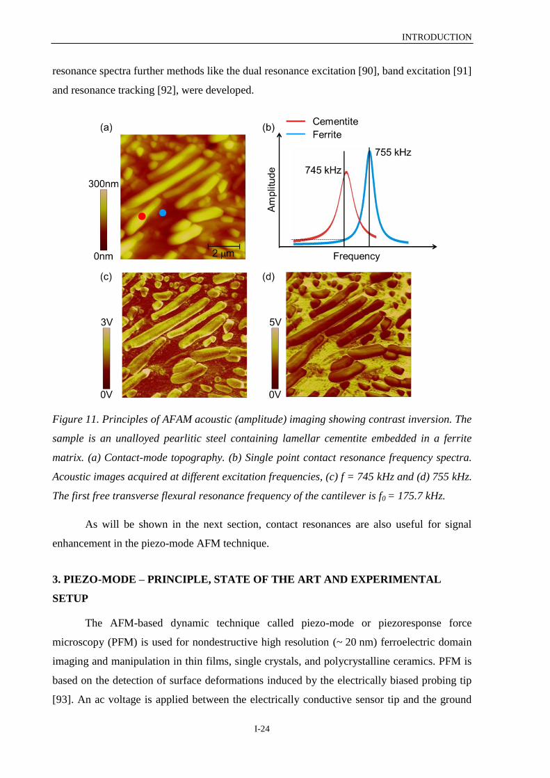
acoustic image. Contrast inversion of acoustic images is observed if the frequency of
excitation is varied between values below and above a contact resonance. Figure 11 presents a
practical example of an unalloyed pearlitic steel containing two phases, lamellar cementite
and ferrite. Figure 11a shows the topography image giving information about the sample
microstructure and surface roughness. The topographic height variation is about 300 nm. Fig.
11b displays a single point contact resonance frequency spectrum. The red and blue curves
represent the contact resonance frequencies for the cementite (745 kHz) and the ferrite
(755 kHz) phases, respectively. Figurec 11c and d show acoustic images acquired at these two
different frequencies. In the acoustic image taken at or close to the lower contact resonance
frequency (Fig. 11c), the cantilever vibration amplitude is higher for the more compliant
phase, here the cementite lamellae. Therefore, the cementite lamellae appear brighter.
Increasing the excitation frequency so that it is at or close to the higher contact resonance
frequency (Fig. 11d), the amplitude of the cantilever decreases on the more compliant phase
and increases on the stiffer one. Hence, the stiffer phase, here the ferrite, appears now
brighter. Thus, a contrast inversion is observed by varying the excitation frequency. If the
excitation frequency is far away from a contact resonance, the contrast disappears completely.
From acoustic images only qualitative information about the sample elastic properties is
obtained. In order to obtain local quantative information, contact resonance frequency
measurements in each image point are necessary. For faster acquisition of the contact
INTRODUCTION
I-24
resonance spectra further methods like the dual resonance excitation [90], band excitation [91]
and resonance tracking [92], were developed.
Figure 11. Principles of AFAM acoustic (amplitude) imaging showing contrast inversion. The
sample is an unalloyed pearlitic steel containing lamellar cementite embedded in a ferrite
matrix. (a) Contact-mode topography. (b) Single point contact resonance frequency spectra.
Acoustic images acquired at different excitation frequencies, (c) f = 745 kHz and (d) 755 kHz.
The first free transverse flexural resonance frequency of the cantilever is f0 = 175.7 kHz.
As will be shown in the next section, contact resonances are also useful for signal
enhancement in the piezo-mode AFM technique.
3. PIEZO-MODE – PRINCIPLE, STATE OF THE ART AND EXPERIMENTAL
SETUP
The AFM-based dynamic technique called piezo-mode or piezoresponse force
microscopy (PFM) is used for nondestructive high resolution (~ 20 nm) ferroelectric domain
imaging and manipulation in thin films, single crystals, and polycrystalline ceramics. PFM is
based on the detection of surface deformations induced by the electrically biased probing tip
[93]. An ac voltage is applied between the electrically conductive sensor tip and the ground

INTRODUCTION
I-25
electrode creating a localized electric field below the tip which interacts with the surface of a
piezoelectric sample via the inverse piezoelectric effect. This voltage (peak-to-peak amplitude
of ~ 10 Vpp) excites a sample vibration (expansion and contraction) locally which is detected
by the cantilever via its sensor tip being in contact with the sample surface. The laser beam
reflected from the cantilever is detected by the four quadrant laser diode of the commercial
AFM microscope, and the signal is then further analyzed using a lock-in technique. Similarly
to AFAM, PFM is carried out in contact mode, and using the low frequency components of
the cantilever deflection with the electronic feedback loop of the AFM, the topography of the
sample is simultaneously acquired. The frequency of the applied voltage is usually lower than
the first transverse flexural resonance frequency of the cantilever (mostly between 10 and
60 kHz). First images at a nanoscale of piezoelectric materials using PFM were presented in
1992 by Güthner and Dransfeld [94]. To date, PFM has found a broad applicability to
ferroelectric domain imaging, domain patterning and spectroscopy in many different materials
such as ferroelectric perovskites [95], piezoelectric III-IV nitrides [96], and recently,
biological systems such as tissues [97,98] and proteins [99].
One distinguishes between vertical (VPFM) and lateral PFM measurements (LPFM).
In a VPFM measurement, the elongation or contraction of the surface (usually a single
domain) is analyzed perpendicularly to the sample surface. Those so-called out-of-plane
signals are obtained mostly via the transverse flexural vibrations of the cantilever and give
information on the out-of-plane component of electromechanical surface response. In a LPFM
measurement, the elongation or contraction of the surface is examined in the plane of the
sample surface. The so-called in-plane signals are obtained mostly via the torsional
movements of the cantilever and give information on the in-plane component of
electromechanical surface response. As mentioned previously, the lock-in technique is used to
analyze the detected signals by comparing those with the excitation signal in terms of
amplitude and phase of the cantilever vibrations. The resulting amplitude is a measure of the
local piezoactivity, and the phase indicates the direction of the domain polarization. Using the
information of VPFM and LPFM signals, the domain polarization, as e.g. in BaTiO3, can be
completely reconstructed [100,101]. Additionally, as discussed by Jungk [102], besides the
transverse flexural and torsional movements, the cantilever can suffer also an independent
third movement called “buckling”. In this case the in-plane force acts perpendicularly to the
tip but in axis with the cantilever (Fig. 12).

INTRODUCTION
I-26
Figure 12. (a) Forces acting on the sensor tip in PFM mode. The three forces Fdefl, Fbuck and
Ftor cause three movements of the cantilever: transverse flexural deflection, buckling and
torsion, respectively (b). The vertical force Fdefl causes a transverse flexural deflection of the
cantilever which is independent of its orientation with respect to the surface normal. Already
in the case of the in-plane forces Ftor and Fbuck, the cantilever response is dependent on the
direction of the driving force with respect to the cantilever axis. While transverse flexural
deflection and buckling are detected as vertical signals, torsion results in a lateral signal on
the photodiode (c). Modified representation according to [102].
Buckling cannot be easily distinguished from a deflection of the cantilever because
both are detected as a vertical signal on the photodiode. Because of the symmetry of the
cantilever, an additional LPFM measurement must then be performed by physically rotating
the sample about 90° [103]. In this way, three components of the piezoresponse signal are
obtained, which allows at least a semiquantitative reconstruction of the polarization
orientation. A complete and precise determination of the polarization directions can be
calculated only if all components of the piezoelectric tensor are known [93]. For further
description of the method the reader is referred to [104-108].
The piezo-mode technique used in this work operates at much higher frequencies
compared to the standard (low frequency) piezoresponse force microscopy technique.
Because of the range of frequencies one operates with (few hundred of kHz to a few MHz) the
technique is named ultrasonic piezo-mode or ultrasonic piezoresponse force microscopy
(UPFM). As in the case of the AFAM technique, UPFM combines AFM with ultrasonics. The
schematic setup used in this work is presented in Fig. 13. The idea to excite contact resonance

INTRODUCTION
I-27
frequencies is similar, but the way to induce the sample vibrations differs considerably. In the
AFAM mode, the high frequency signal of the function generator is connected to the
ultrasonic transducer below the sample. Longitudinal waves are emitted which causes out-of-
plane surface vibrations that are sensed by the cantilever via its sensor tip. As described
earlier, contact resonance frequencies are excited. This can be used to measure local elastic
properties. In the UPFM mode, the high frequency signal of the function generator is
connected directly to the electrically conductive AFM-cantilever, and the tip-sample vibration
is excited via the inverse piezoelectric effect. Like in the AFAM mode, the operation
frequency is set close to a contact resonance frequency of the system. The piezo-mode signal
is thus enhanced through resonance amplification [85]. For the vertical (out-of-plane) surface
displacements, the excitation frequency is set close to a transverse flexural contact resonance
of the cantilever. In the case for the lateral (in-plane) surface displacements, the excitation
signal is set close to a torsional contact resonance of the cantilever. Similar to the standard
(low frequency) PFM, amplitude and phase images are taken for information about the piezo
activity of the sample. In order to allow local poling experiments with subsequent imaging of
induced changes, a DC-power supply is also connected to the system (Fig. 13).
Figure 13. Schematic set-up showing the combined AFAM and UPFM techniques. The AFM
cantilever is in contact with the piezoelectric sample surface. The contact resonance modes of
the beam are excited by surface displacements caused by: (1) longitudinal waves emitted from
an ultrasonic transducer (AFAM mode); (2) due to the inverse piezoelectric effect when an
alternating electrical voltage is applied directly to the AFM cantilever and tip (piezo-mode).
A connected DC-power supply allows also the manipulation of the ferroelectric domains.
Modified representation according to [85,109].
Experiments are made in two steps. In a first step, a DC voltage of variable amplitude
and poling direction is applied between the tip and the sample while the sample is scanned. In
a second step, the same area is imaged in the UPFM mode to check whether the PFM contrast

INTRODUCTION
I-28
is changed locally. An increased contrast in the UPFM amplitude image corresponds to an
increased piezo activity.
4. RESEARCH OVERVIEW
4.1 Structural steels
The main objective of the first and largest part of this thesis is to identify the
mechanisms governing and/or contributing to the magnetization process of steels containing
different phases at the micro- and nanoscale in order to support the evaluation of macroscopic
electromagnetic and micromagnetic nondestructive methods. Analysis and interpretation of
the observed macroscopic electromagnetic and micromagnetic nondestructive output signals
require an understanding of the underlying domains and their interactions with the
microstructure. The observation and characterization of the magnetic microstructure and its
dynamics is therefore crucial to reveal the mechanisms controlling the magnetization
processes in multiphase steels.
In the work described in chapters II-VI (publications A-E), samples of a high purity
polycrystalline iron and of two unalloyed pearlitic steels (Fe-0.8%C and Fe-1.5%C)
containing globular and lamellar cementite embedded in a ferrite matrix have been chosen as
model systems. To study the relative influences of the ferrite and cementite phases on the
macroscopic electromagnetic and micromagnetic measurement signals an approach based on
macroscopic measurement signals as well as the observation and characterization of the
material in the micro- and nanoscale is applied. At the macroscopic scale, magnetic hysteresis
loops and magnetic Barkhausen noise are used for materials characterization and evaluation.
At the micro- and nanoscopic scale, a relevant magnetic imaging technique for NDT&E,
namely MFM, is used for magnetic domains visualization and also for the detection of
different micromagnetic events.
A setup based on an electromagnet, a pick-up coil, and a magnetic field sensor was
used to measure magnetic hysteresis loops and magnetic Barkhausen noise of the high purity
polycrystalline iron and unalloyed pearlitic steel samples, the latter containing different
proportions of ferrite and cementite phases. A system composed of a commercial MFM
microscope coupled with an external coil providing a controllable external magnetic field was
built. Applying this setup, the influence of the cementite and ferrite phases on the
magnetization processes and also on the detected Barkhausen signals was investigated. The
characterization of local micromagnetic events in a thick (bulk) polycrystalline sample
requires a surface in which the grains are suitably oriented with regard to their easy axes of

INTRODUCTION
I-29
magnetization. Using the EBSD technique, the crystalline orientations of grains in both, the
ferrite and the cementite phases, were determined. Local elastic properties of the ferrite and
cementite phases were probed with a resolution down to the nm range using the AFAM
technique. By combining the MFM, AFAM and EBSD techniques, the local magnetic, elastic,
and crystallographic microstructure of the investigated unalloyed pearlitic steels were
examined.
Chapter II (publication A, peer-reviewed paper) shows in detail the use of the MFM
under a controllable external applied field to image the magnetic microstructures of the high
purity polycrystalline iron and the Fe-0.8%C and Fe-1.5%C samples. Focus is given in the
magnetization process in the ferrite, reversible and irreversible domain wall movements are
observed, and different interactions of the domain walls in the ferrite matrix with the
cementite precipitates are revealed.
Chapter III (publication B, peer-reviewed paper) shows how one can optimize the
macroscopic measurement setup in order to identify the ferrite and the cementite phases in the
Fe-0.8%C and Fe-1.5%C samples on the MBN profiles. MFM under a controllable external
applied field is used to study the magnetic microstructure in the Fe-1.5%C sample with
special emphasis to the process related to the magnetization of the cementite phase.
Chapter IV (publication C, paper submitted to Ultramicroscopy) proposes a new
method to determine the magnetic easy axes of micro- and nanoscopic ferromagnetic
precipitates embedded in a bulk material by combining the MFM and EBSD techniques. It
also shows how different types of magnetic probes can influence the contrast in the magnetic
images. As examples, the Fe-0.8%C and Fe-1.5%C samples which contain globular and
lamellar cementite precipitates in a ferrite matrix are chosen.
Chapter V (publication D, conference paper) describes the dynamics of the magnetic
microstructure imaged by MFM of the high purity polycrystalline iron and the Fe-1.5%C
samples. Particular attention is given to the magnetization process of the high purity iron
sample. The domain wall movements in this sample are initiated by much weaker applied
field compared to those necessary on the Fe-1.5%C sample. It demonstrates how the
crystalline orientation of the grains in the high purity iron sample influences their surface
domain configurations.
Chapter VI (publication E, conference paper) presents the magnetic microstructure and
the local elastic properties of the Fe-0.8%C sample. Additionally, the AFAM technique is
used to image the microstructure and probe mechanical properties on the micro- and
nanoscale of austenitic twinning induced plasticity (TWIP) steels. Quantitative indentation

INTRODUCTION
I-30
modulus results were obtained as a function of the grain orientations and compared to the
results obtained using the nanoindentation technique. Finally, important insights in the
deformation mechanisms were examined via surface relief analysis obtained by AFM during
plastic deformation.
4.2 Functional lead-free ceramics
The main objective of the second much shorter part of this thesis, carried out together
with the BisNano project partners [2], is the evaluation of the functionalities of bismuth-based
materials for a variety of industrial applications, as e.g. lead-free ferroelectrics and
piezoelectrics. The design and engineering of new functional lead-free ferro- and piezoelectric
materials requires a thorough understanding of the micro- and nanostructure related
properties.
Chapter VII (publication F, peer-reviewed paper) describes ferroelectric epitaxial thin
film samples of bismuth ferrite (BiFeO3) which were grown in different crystallographic
orientations (100), (110), and (111). The quality of the films was evaluated using X-ray
diffraction (XRD) and AFM. To study the influence of the crystallographic orientation of the
films on the ferroelectric domain patterns, low frequency (standard) PFM and UPFM were
used. In order to examine local polarization switching, an additional dc-power supply was
connected to the PFM/UPFM system. Finally, AFAM was employed to probe the local elastic
properties of the films at a nanoscale by acquiring surface elasticity maps.
Promising candidates for lead-free piezoelectric materials were investigated at a
macro-, micro- and nanoscale (chapter VIII, publication G, part of the EU-Mexico BisNano
project report). Different lead-free bismuth-based bulk ceramics like Bi0.5Na0.5TiO3 (BNT),
0.94Bi0.5Na0.5TiO3-0.06BaTiO3 (BNT-BT), Mn-doped BNT-BT, and Sr-doped BNT-BT were
synthesized via conventional mixed oxide route and sintering. Macroscopic properties like
piezoelectric coupling coefficients and elastic constants were determined using impedance
and ultrasound measurements, respectively. Laser vibrometry was used for the identification
of sample resonances and also for the measurements of the maximal surface vibration
amplitudes of the ceramic samples at their resonances. Micro- and nanoscopic investigations
were performed using AFM, AFAM and UPFM. AFM contact mode was used to examine
first the quality of the sample surfaces with regard to roughness and cleanliness. AFAM and
UPFM were used to image at a nanoscale surface elastic properties and ferroelectric domains,
respectively. Finally, the most promising lead-free bismuth-based bulk ceramic samples were
successfully tested as ultrasonic transducer materials.
INTRODUCTION
I-31
REFERENCES
[1] EU-Directive 2002/95/EC: Restriction of the Use of Certain Hazardous Substances in
Electrical and Electronic Equipment (RoHS)“, Official Journal of the European Union 46
(2003) 19.
[2] EC-FP7 Call: NMP.2010.1.2-4 Adding Value to mining at the Nanostructure level,
Project: Functionalities of Bismuth-based nanostructures (BisNano) 263878.
[3] D.I. Gordon, Reviews of Modern Physics 25 (1953) 56.
[4] A.H. Geisler, Reviews of Modern Physics 25 (1953) 316.
[5] G.A. Matzkanin, R.E. Beissner, E.M. Teller “The Barkhausen effect and its Application to
Nondestructive Evaluation”, in: Nondestructive Testing Information Analysis Center, (San
Antonio, Texas, NTIAC report 79-2, 1979).
[6] O. Kanji, G. Dobmann, “Nondestructive Testing, 5. Magnetic and Electromagnetic
Engineering”, in Ullmann's Encyclopedia of Industrial Chemistry, (Weinheim, John Wiley &
Sons, 2000).
[7] I. Altpeter, R. Becker, G. Dobmann, R. Kern, W. Theiner, A. Yashan, Inverse Problems
18 (2002) 1907.
[8] D.C. Jiles, Journal of Physics D: Applied Physics 21 (1988) 1186.
[9] H. Kronmüller, “Magnetisierungskurve der Ferromagnetika”, in: Moderne Probleme der
Metallphysik, Vol. 2, ed. by A. Seeger (Springer, Berlin, 1966) 24-156.
[10] D.C. Jiles, NDT & E International 21 (1988) 311.
[11] A. Dumay, Dissertation, Ecole des Mines, Nancy, France (2008).
[12] L. Batista, U. Rabe, S. Hirsekorn, NDT & E International 57 (2013) 58.
[13] C. Boller, I. Altpeter, G. Dobmann, M. Rabung, J. Schreiber, K. Szielasko, R.
Tschuncky, Materialwissenschaft und Werkstofftechnik 42 (2011) 269.
[14] G. Dobmann, R. Becker, W.A. Theiner, “Progress in the Micromagnetic Multi-parameter
Microstructure and Stress Analysis (3MA)”, in Non-Destructive Characterization of
Materials, vol 3, P. Höller, V. Hauk, G. Dobmann, C. Ruud, R. Green, Eds. (Berlin: Springer)
(1989) 516.
[15] K. Szielasko, Entwicklung messtechnischer Module zur merhparametrischen
elektromagnetischen Werkstoffcharakteriesierung und prüfung, Dissertation, Saarland
University, Saarbrücken (2009).
[16] K. Szielasko , I. Mironenko , I. Altpeter, H.-G. Herrmann, C. Boller, IEEE Transactions
on Magnetics 49 (2013) 101.
[17] I. Altpeter, W. Theiner, M. Gessner, Vorrichtung zum ortsaufgelösten zerstörungsfreien

INTRODUCTION
I-32
Untersuchungen vom magnetischen Kenngrößen, European Patent Nr. EPO 595 117B1,
04.05. 1994.
[18] I. Altpeter, G. Dobmann, N. Meyendorf, H. Blumenauer, D. Horn, M. Krempe,
Proceedings of the International Symposium on Nondestructive Characterization of Materials
8, Boulder/Colorado, USA (1997) 659.
[19] M. Sheikh-Amiri, K. Szielasko, I. Altpeter, C. Boller, D. Fischer, J. Hahn, IOP Conf.
Series: Materials Science and Engineering 31 (2012) 012021.
[20] E. Hanke, “Prüffung Metallischer Werkstoffe”, (Leipzig,VEB Deutscher Verlag für
Grundstoffindustrie, Band 2, 1960).
[21] B.D. Cullity, Introduction to magnetic materials, (London, Addison Wesley, 1972).
[22] D.K. Bhattacharya, Magnetic NDT for the Characterization of Industrial Materials,
Materials Characterization Techniques – Principles and Applications, Eds.: G. Sridhar, S.
Ghost Chowdhury & N.G. Goswami, NML, Jamshedpur-831007 (1999) 210-227.
[23] V. Moorthy, S. Vadyanathan, T. Jayakumar, B. Raj, Journal of Magnetism and Magnetic
Materials 171 (1997) 179.
[24] O. Saquet, J. Chicois, A. Vincent, Materials Science and Engineering A 269 (1999) 73.
[25] M.J. Sablik, B. Augustyniak, “Magnetic methods of nondestructive evaluation”, in:
Wiley Encyclopedia of Electrical and Electronics Engineering Vol. 12, ed. by Wiley & Sons,
(New York, 1999) 12-31.
[26] VDI/VDE – Richtlinie 2616, Blatt 1, Härteprüfung an metallischen Werkstoffen,
Düsseldorf: VDI (2012) 30-35.
[27] G. Dobmann, I. Altpeter, M. Kopp, Russian Journal of Nondestructive Testing 42
(Compendex) (2006) 272.
[28] G. Dobmann, I. Altpeter, K. Szielasko, M. Kopp, Journal of Theoretical and Applied
Mechanics 44 (Copyright 2006, The Institution of Engineering and Technology) (2006) 649.
[29] S. Takaya, I. Yamagata, S. Ichikawa, Y. Nagae, K. Aoto, International Journal of
Applied Electromagnetics and Mechanics 33 (2010) 1335.
[30] D.-G. Park, I.-G. Park, W.-W. Kim, Y.-M. Cheong, J.-H. Hong, "Nuclear Engineering
and Design 238 (Compendex) (2008) 814.
[31] L. Debarberis, B. Acosta, A. Zeman, S. Pirfo, P. Moretto, A. Chernobaeva, Y. Nikolaev,
International Journal of Microstructure and Materials Properties 2 (Copyright 2008, The
Institution of Engineering and Technology) (2007) 326.

INTRODUCTION
I-33
[32] J.S. McCloy, R.O. Montgomery, P. Ramuhalli, R.M. Meyer, S. Hu, C.H. Henager Jr.,
B.R. Johnson, “Materials degradation and detection (MD2): Deep Dive Final Report”, PNNL-
22309 (2013).
[33] P. Weiss, Journal de Physique 6 (1907) 661.
[34] F. Bitter, Physical Review 38 (1931) 1903.
[35] L.D. Landau, E. Lifshitz, Physikalische Zeitschrift der Sowjetunion 8 (1935) 153.
[36] S. Chikazumi, “Physics of Magnetism”, (New York, Wiley, 1964).
[37] G. Bertotti, “Hysteresis in Magnetism – For Physicists, Materials Scientists, and
Engineers”, (San Diego, CA, Academic Press, Inc., 1998).
[38] R. Becker, W. Döring, “Ferromagnetismus”, (Berlin, Springer, 1939).
[39] R.M. Bozorth, “Ferromagnetism”, (New York, IEEE Press, 1951).
[40] D.C. Jiles, “Introduction to Magnetism and Magnetic Materials (2nd
Ed.)”, (London,
Chapman & Hall, 1998).
[41] D.C. Jiles, Journal of Physics D: Applied Physics 21 (1988) 1196.
[42] H. Barkhausen, Physikalische Zeitschrift 20 (1919) 401.
[43] A.E. Lord, “Acoustic Emission”, in Physics Acoustics, Vol. XI, ed. by W.P. Mason, R.N.
Thurston, (New York, Academic Press, 1975).
[44] K. Tiito, “Solving Residual Stress Measurement Problems by a New Nondestructive
Magnetic Method”, in: Nondestructive Evaluation: Application to Materials Processing, ed.
by O. Buck, S.M. Wolf, (Ohio, ASM, Materials Park, 1984).
[45] V.A. Yardley, Magnetic detection of microstructural change in power plant steels,
Dissertation, Cambridge University, Cambridge (2003).
[46] J.W. Lau, J.M. Shaw, Journal of Physics D: Applied Physics 44 (2011) 303001.
[47] C.A. Kittel, Physical Review 76 (1949) 1827.
[48] H. Ebert, Reports on Progress in Physics 59 (1996) 1665.
[49] Z.Q. Ziu, S.D. Bader, Review of Scientific Instruments 71 (2000) 1243.
[50] B.C. Choi, M. Belov, W.K. Hiebert, G.E. Ballentine, M.R. Freeman, Physics Review
Letters 86 (2001) 728.
[51] H. Boersch, H. Raith, Naturwissenschaften 46 (1959) 574.
[52] M.E. Hale, H.W. Fuller, H. Rubinstein, Journal of Applied Physics 30(5) (1959) 789.
[53] N.F. Mott, Proceedings of the Royal Society A 124 (1929) 425.
[54] J. Kessler, “Polarized Electrons”, (Berlin, Springer, 1985).
[55] A.M. Chang, H.D. Hallen, L. Harriott, H.F. Hess, H.L. Kao, J. Kwo, R.E. Miller, R.
Wolfe, J. van der Ziel, T.Y. Chang, Applied Physics Letters 61 (1992) 1974.

INTRODUCTION
I-34
[56] Y. Martin, H.K. Wickramasinghe, Applied Physics Letters 50 (1987) 1455.
[57] J.J. Saenz, N. Garcia, P. Grütter, E. Meyer, H. Heinzelmann, R. Wiesendanger, L.
Rosenthaler, H. R. Hidber, H. J. Güntherodt, Journal of Applied Physics 62 (1987) 4293.
[58] X. Zhu, P. Grütter, V. Metlushko, B. Ilic, Journal of Applied Physics 91 (2002) 7340.
[59] R. Proksch, E. Runge, P.K. Hansma, S. Foss, Journal of Applied Physics 78 (1995) 3303.
[60] A. Hubert, R. Schäfer, “Magnetic domains – the analysis of magnetic microstructures”,
(Berlin, Springer; 1998).
[61] H. Kronmüller, S. Parkin, “Handbook of magnetism and advanced magnetic materials”,
vol 2., Micromagnetism, (New York, Wiley & Sons, 2007).
[62] M. Coisson, F. Vinai, P. Tiberto, F. Celegato, Journal of Magnetism and Magnetic
Materials 321 (2009) 806.
[63] S. Huo, J.E.L. Bishop, J.W. Tucker, M.A. Al-Khafaji, W.M. Rainforth, H.A. Davies, et
al., Journal of Magnetism and Magnetic Materials 190 (1998) 17.
[64] L. Zhang, B. An, S. Fukuyama, T. Iijima, K. Yokogawa, Journal of Applied Physics 108
(2010) 063526.
[65] S. Takaya, T. Suzuki, Y. Matsumoto, K. Demachi, M. Uesaka, Journal of Nuclear
Materials 327 (2004) 19.
[66] M.G. Hetherington, J.P. Jakubovics, J.A. Szpunar, B.K. Tanner, Philosophical Magazine
B 56 (1987) 561.
[67] S.M. Thompson, B.K. Tanner, Journal of Magnetism and Magnetic Materials 123 (1993)
283.
[68] C.C.H. Lo, C.B. Scruby, Journal of Applied Physics 85 (1999) 5193.
[69] C.C.H. Lo, J.P. Jakubovics, C.B. Scruby, Journal of Applied Physics 81 (1997) 4069.
[70] C.C.H. Lo, J.P. Jakubovics, C.B. Scruby, IEEE Transactions on Magnetics 33 (1997)
4035.
[71] A.D. Beale, J.P. Jakubovics, M.G. Hetherington, C.B. Scruby, B.A. Lewis, K.J. Davies,
Journal of Magnetism and Magnetic Materials 104-107 (1992) 365.
[72] J.W. Lau, M.A. Schofield, Y. Zhu, Ultramicroscopy 107 (2007) 396.
[73] U. Rabe, W. Arnold, Applied Physics Letters 64 (1994) 1493.
[74] U. Rabe, K. Janser, W. Arnold, Review of Scientific Instruments 67 (1996) 3281.
[75] D.C. Hurley, M. Kopycinska-Müller, A.B. Kos, R.H. Geiss, Advanced Engineering
Materials 7 (2005) 713.
[76] K. Yamanaka, H. Ogiso, O.V. Kolosov, Applied Physics Letters 64 (1994) 178.
[77] G. Binning, C.F. Quate, C. Gerber, Physics Review Letters 56 (1986) 930.

INTRODUCTION
I-35
[78] D.C. Hurley, “Contact Resonance Force Microscopy Techniques for Nanomechanical
Measurements”, in: Applied Scanning Probe Methods Vol. XI, ed. by H. Fuchs, B. Bhushan,
(Berlin, New York, 2009) 97-138.
[79] U. Rabe, “Atomic Force Acoustic Microscopy”, in: Applied Scanning Probe Methods II,
ed. by H. Fuchs, B. Bhushan., (Berlin, Springer, 2006) 37-90.
[80] U. Rabe, M. Kopycinska-Müller, S. Hirsekorn, "Atomic Force Acoustic Microscopy", in:
Acoustic Scanning Probe Microscopy, ed. by F. Marinello, D. Passeri, E. Savio, (Berlin,
Springer, 2013) 123-153.
[81] U. Rabe, S. Amelio, E. Kester, V. Scherer, S. Hirsekorn, W. Arnold, Ultrasonics 38
(2000) 430.
[82] K.L. Johnson, “Contact Mechanics”, (Cambridge, U.K.,Cambridge University Press,
1985) 84-99.
[83] B. Cappella, G. Dietler, Surface Science Reports 34 (1999) 1.
[84] J.J. Vlassak, W.D. Nix, Philosophical Magazine A 67 (1993) 1045.
[85] U. Rabe, M. Kopycinska, S. Hirsekorn, J. Muñoz-Saldaña, G.A. Schneider, W. Arnold,
Journal of Applied Physics D: Applied Physics 35 (2002) 2621.
[86] U. Rabe, S. Amelio, M. Kopycinska, M. Kempf, M. Göken, W. Arnold, Surface and
Interface Analysis 33 (2002) 65.
[87] M. Kopycinska-Müller, On the elastic properties of nanocrystalline materials and the
determination of elastic properties on a nanoscale using the atomic force acoustic microscopy
technique. Saarbrücken: PhD thesis, Science and Technical Faculty III, Saarland University
and IZFP report No. 050116-TW, 2005.
[88] B. Gronau, Bandanregung in der Ultraschall-Kraftmikroskopie. Saarbrücken: Diploma
thesis, Science and Technical Faculty II, Saarland University and IZFP report No. 130107-
TW, 2012.
[89] S. Amelio, A. V. Goldade, U. Rabe, V. Scherer, B. Bhushan, and W. Arnold, Thin Solid
Films 392 (2001) 75.
[90] M. Kopycinska-Müller, A. Striegler, R. Schlegel, N. Kuzeyeva, B.Köhler, Review of
Scientific Instruments 83 (2012) 043703.
[91] S. Jesse, S.V. Kalinin, R. Proksch, A.P. Baddorf, B.J. Rodriguez, Nanotechnology 18
(2007) 435503.
[92] A.B. Kos, D.C. Hurley, Measurement Science and Technology 19 (2008) 015504.
[93] A. Kholkin, S.V. Kalinin, A. Roelofs, A. Gruverman, “Review of Ferroelectric Domain
Imaging by Piezoresponse Force Microscopy”, in: Scanning Probe Microscopy: Electrical

INTRODUCTION
I-36
and Electromechanical Phenomena at the Nanoscale, ed. by S. V. Kalinin, A. Gruverman,
(New York, Springer, 2007) 173-214.
[94] P. Güthner, K. Dransfeld, Applied Physics Letters 61 (1992) 1137.
[95] A. Gruverman, O. Auciello, H. Tokumoto, Annual Review of Materials Science 28
(1998) 101.
[96] B.J. Rodriguez, A. Gruverman, A.I. Kingon, R.J. Nemanich, O. Ambacher, Applied
Physics Letters 80 (2002) 4166.
[97] C. Halperin, S. Mutchnik, A. Agronin, M. Molotskii, P. Urenski, M. Salai, G. Rosenman,
NanoLetters 4 (2004) 1253.
[98] S.V. Kalinin, B.J. Rodriguez, S. Jesse, T. Thundat, V. Grichko, A.P. Baddorf, A.
Gruverman, Ultramicroscopy 106 (2006) 334.
[99] A. Gruverman, B.J. Rodriguez, S.V. Kalinin, “Electromechanical Behavior in Biological
Systems at the Nanoscale”, in: Scanning Probe Microscopy: Electrical and
Electromechanical Phenomena at the Nanoscale, ed. by S. V. Kalinin, A. Gruverman, (New
York, Springer, 2007) 615-633.
[100] L.M. Eng, H.-J. Gütherodt, G.A. Schneider, U. Köpke, J. Muñoz-Saldaña, Applied
Physics Letters 74, (1999) 233.
[101] J. Muñoz-Saldaña, G.A Schneider, L.M Eng, Surface Science Letters 480 (2001) L402.
[102] T. Jungk, Á. Hoffmann, E. Soergel, in Ferroelectric Crystals for Photonic Applications,
ed. by P. Ferraro, S. Grilli, P.D. Natale, (Berlin, Springer, 2014) 205-226.
[103] B.J. Rodriguez, A. Gruverman, A.I. Kingon, R.J. Nemanich, J.S. Cross, Applied Physics
A 80 (2005) 99.
[104] L.M. Eng., Nanotechnology 10 (1999) 405.
[105] S. Hong, J. Woo, H. Shin, J.U. Jeon, Y.E. Pak, E.L. Colla, N. Setter, E. Kim, K. No,
Journal of Applied Physics 89 (2001) 1377.
[106] C. Harnagea, A. Pignolet, M. Alexe, D. Hesse, Integrated Ferroelectrics 44 (2002) 113.
[107] S.V. Kalinin, R. Shao, D.A. Bonnell, Journal of the American Ceramic Society 88
(2005) 1077.
[108] S.V. Kalinin, D.A. Bonnell, “Electric Scanning Probe Imaging and Modification of
Ferroelectric Surfaces”, in: Nanoscale characterization of Ferroelectric Materials, ed. by M.
Alexe, A. Gruverman, (Berlin, Springer, 2004) 1-39.
[109] U. Rabe, "Ultraschall-Kraftmikroskopie - Prinzip und Anwendung", in Fortschritte der
Akustik (DAGA, Dresden, 2008).

I-37


PUBLICATION A
II-1
II. MAGNETIC MICRO- AND NANOSTRUCTURES OF UNALLOYED STEELS:
DOMAIN WALL INTERACTIONS WITH CEMENTITE PRECIPITATES
OBSERVED BY MFM (PUPLICATION A)
L. Batista, U. Rabe, and S. Hirsekorn
NDT & E International (2013) Vol. 57; 58-68.
ABSTRACT. The morphology and content of a cementite phase controls the macroscopic
mechanical and magnetic properties of steels. The influence of the cementite content on the
bulk magnetic properties in unalloyed steels was observed in hysteresis loop and Barkhausen
noise signals. Globular cementite embedded in a ferrite matrix is characterized by atomic
force microscopy and magnetic force microscopy. Size, shape and orientation of the grains
influence the domain configuration. When an external magnetic field is applied, the
magnetization process occurs mainly in the ferrite matrix. The Bloch walls in the ferrite
matrix move, and they are pinned by the cementite precipitates. This microscopic observation
correlates with the macroscopic magnetic properties of the investigated material.
Keywords: Atomic force microscopy (AFM), Magnetic force microscopy (MFM), Steel,
Magnetic domains, Barkhausen noise, Microstructure, Non-destructive testing

PUBLICATION A
II-2
1. INTRODUCTION
Steels continue to be one of the most important structural material several millennia
after their discovery. Two prominent phases in steels are ferrite and cementite (Fe3C), a
metastable narrow-composition-field intermetallic compound with an orthorhombic
symmetry. Cementite is important because its morphology and volume fraction directly
controls mechanical and magnetic properties of steels. For quality control and assurance the
mechanical properties of steels as well as the morphology and content of the cementite phase
can be monitored using electromagnetic non-destructive testing methods. These methods are
based on a correlation between mechanical and magnetic properties and deliver parameters on
a macroscopic scale.
The bulk macroscopic magnetic properties and Barkhausen noise profile curves of
unalloyed steels have already been studied by many authors. It was shown that the carbon
content influences the shape of the hysteresis loop and the Barkhausen noise signals generated
by a microstructure containing globular cementite embedded in a ferrite matrix [1,2].
Amplitude and shape of the Barkhausen signal change with the addition of a small amount of
carbon, i.e. solid solution in iron [3]. Thompson and Tanner [4] discussed the influence of the
amount of pearlite phase on the magnetic and mechanical hardness. However, all these
macroscopic observations rely on a phenomenological description of the interactions of the
magnetic domains with the microstructure. Fundamental nano- and microscopic investigations
are still researching theoretically and experimentally the phenomena associated to such
interactions, e.g. the pinning effect of domain walls by magnetic inclusions.
The magnetic domain structures can be imaged by different techniques. For example,
the Bitter technique was used to examine the configuration of the magnetic domains in
magnetite [5]. Domains in high-permeability materials were imaged by Kerr microscopy [6],
the domain configuration of a cementite thin foil was revealed by Lorentz electron
microscopy [7], and recently a domain structure was imaged in three dimensions by Neutron
diffraction tomography [8]. Magnetic force microscopy (MFM) has been widely employed to
map magnetic structures of surfaces [9]. In addition to its outstanding local resolution of up to
10 nm MFM has other advantages [10]: Topography and magnetic structure can be
simultaneously measured allowing the study of interaction between defects and magnetic
properties, and MFM can be performed under various environmental conditions. Since
magnetostatic interactions are long-range, MFM is less sensitive to surface contamination
than other scanning probe techniques, and the surface preparation is relatively easy. Different
reviews of the principles and methods of MFM were published [11-13]. Most studies of

PUBLICATION A
II-3
domain structures with MFM focused on thin magnetic layers [14-16], and only few studies
used MFM to image the domain structure of polycrystalline bulk materials [17].
In this paper, samples of a high purity polycrystalline iron and of two unalloyed steels
(Fe-0.8%C and Fe-1.5%C) containing globular cementite embedded in a ferrite matrix have
been chosen as model systems. In the first part of this work, the macroscopic magnetic
quantities, i.e. saturation magnetization, coercive field and maximum Barkhausen noise
amplitude were measured and interpreted with respect to the microstructural state. In the
second part, the magnetic microstructures were observed using a magnetic force microscope.
The MFM was coupled with an external coil providing a controlled in-plane magnetic field
which allowed the observation of the dynamic behavior of the magnetic domains.
Ferromagnetic domains were studied in the high purity polycrystalline iron sample and in the
cementite and ferrite phases of the unalloyed steels. By means of electron backscatter
diffraction (EBSD) the crystalline orientation of the cementite particles and the ferrite phase,
respectively, was determined. The correlation between the macroscopic magnetic properties
and the magnetic and crystallographic microstructure was examined.
2. BACKGROUND OF THE MEASUREMENT METHODS
2.1 Macroscopic magnetic methods
Ferromagnetic materials consist of small finite uniformly magnetized regions called
magnetic domains. Each domain is spontaneously magnetized to the saturation value of the
material. Domain walls separate neighboring domains of different magnetization orientations.
The driving energy for formation of domains in a macroscopic ferromagnetic material is the
stray field energy. The reduction of the stray field energy is accompanied by an increase of
the total domain wall energy. The equilibrium state therefore is characterized by the minimum
of the total energy, i.e. stray field plus domain wall energy [18,19]. In the magnetic structure
of a bulk ferrous magnetic material only two kinds of domain walls are observed: 180° -
Bloch walls (BWs) which are magnetostrictively inactive, have short range stress fields
resulting in high mobility and sensitivity to external stress, and 90°-BWs which are
magnetostrictively active, have long-range stress fields and therefore low mobility. The Bloch
wall movement takes place discontinuously because BWs are temporarily pinned by
microstructural obstacles like dislocations, precipitates and phase or grain boundaries in a
polycrystalline material. The stepwise pull-out of the walls from the obstacles which changes
the magnetization state locally is called “Barkhausen event” or “-jump”. These local
magnetization changes induce pulsed eddy currents into the sample which are detected as

PUBLICATION A
II-4
electrical voltage pulses in a pick-up coil near the surface, the so called Barkhausen noise
[20]. Macroscopic magnetic properties including coercive field, permeability, residual
induction and power loss derived from hysteresis loop and Barkhausen signals allow
characterization of the microstructural state of ferromagnetic materials.
In the experimental set-up used here, the magnetic field for hysteresis loop and
Barkhausen noise measurements was generated by an electromagnet which was connected to
a computer-controlled bipolar power supply (Fig. 1). Cylindrical samples with a diameter of 8
mm and length of 50 mm were magnetized along their axial direction. A maximum magnetic
field strength H of 130 A/cm was reached at an excitation frequency of 0.05 Hz. The
magnetic tangential field strength H was measured by a Hall probe. The change in magnetic
flux density B and the inductive Barkhausen noise amplitude M were measured by a pick-up
coil surrounding the sample (Fig. 1). The envelope of the noise signals (analyzing frequency
fA = 200 Hz - 50 kHz) and the magnetic flux density were recorded as a function of the
tangential field strength.
Figure 1. (a) Schematic sketch of the experimental set-up for hysteresis loop and Barkhausen
noise measurements, (b) schematic hysteresis loop with coercive field HC, Magnetic flux at
saturation BS, and remnant magnetic flux BR, (c) schematic Barkhausen noise curve with
maximum of Barkhausen noise amplitude Mmax, remnant Barkhausen noise amplitude MR, and
coercive field Hcm deduced from Barkhausen noise curve.

PUBLICATION A
II-5
2.2 Magnetic force microscopy with a superposed external magnetic field
Magnetic force microscopy [21,22] is a special dynamic mode of atomic force
microscopy [23] in which a magnetic sample is scanned with a micro fabricated silicon
cantilever coated with a thin layer (thickness < 50 nm) of ferromagnetic material (Fig. 2). A
sharp sensor tip with an apex diameter in the nm range is attached to the cantilever. The
cantilever is deflected by the magnetic interaction force F between the ferromagnetic tip and
the stray field emanating from the sample surface:
( ) , (1)
where m is the magnetic moment of the tip and HSam is the magnetic stray field of the sample.
Since the magnetization of the tip is parallel to its axis, only the stray field component
perpendicular to the sample surface is detected. Thus, the force Fz acting in the z-direction is
( )
. (2)
A beam deflection position detector measures the bending of the cantilever. MFM
provides simultaneously an image of the topography and a map of the magnetic
microstructure of the specimen surface. Every image line is scanned twice, and the cantilever
is vibrated close to its resonance frequency during the scan. First the surface profile is
recorded in the intermittent contact mode (Tapping mode) [24]. In the second run, the line is
scanned once more at an adjustable distance above the previously measured topographic
profile. Due to the magnetic force gradient the cantilever experiences a shift in amplitude and
phase at its frequency of vibration. The topography and phase signals are displayed as color
coded images in a computer. The advantage of the lifting procedure is the automatic
subtraction of surface features from the total image leaving primarily magnetic information.
The typical lift height ranges from 10 nm to 100 nm [25]. A lift height of 60-80 nm was
chosen for all MFM measurements reported here. All magnetic images presented in this work
are phase images, i.e. the local phase shift was recorded as a function of position.
A commercial MFM instrument (Nanoscope III®
multimode, Digital Instruments,
Santa Barbara, CA, USA) was used. The sensor tips were CoCr-coated with a coercivity of
~ 318.4 A/cm (~ 400 Oe) (MESP, Bruker AXS Inc., Madison, WI, USA). An external
electromagnet was combined with the MFM (Fig. 2). The pole shoes of the electromagnet
were adjusted such that the sample inside the AFM was magnetized parallel to its surface.

PUBLICATION A
II-6
Figure 2. Experimental set-up for the MFM measurements coupled with an external coil
providing a controlled in-plane magnetic field.
3. INVESTIGATED MATERIALS
Samples of high purity iron (99.99%) and of two unalloyed steels, Fe-0.8%C and Fe-
1.5%C, containing globular cementite (Fe3C) in a ferrite matrix were examined. The samples
were provided as-cast and machined in a cylindrical shape of 8 mm diameter and 50 mm
length. In order to remove all processing-induced residual stresses, the samples were vacuum
annealed at 600°C for 4h. Scanning electron microscopy (SEM) images (Fig. 3) show the
microstructure of the Fe-0.8%C and Fe-1.5%C samples. The size of the cementite precipitates
ranges from a few hundred nanometers to about 10 m in diameter. The average grain size is
approximately 80 m for all samples.
For AFM and MFM measurements small specimens (3 x 3 x 1 mm3) were cut from the
annealed cylindrical samples by spark erosion and mechanically polished by standard
procedures. Directly before the measurements, the samples were slightly etched using Nital
(95% ethanol + 5% nitric acid) in order to obtain suitably reproducible surface conditions.

PUBLICATION A
II-7
Figure 3. SEM images showing the microstructure of the investigated samples with cementite
precipitates: (a) Fe-0.8%C and (b) Fe-1.5%C.
4. RESULTS AND DISCUSSION
4.1 Bulk magnetic properties
The magnetic hysteresis curves of the three samples are shown in Figures 4a-c (dotted
lines). The coercivity Hc increases with carbon content, while the relative permeability at the
coercive field Hc, the remanence BR, and the saturation magnetization BS at 100 A/cm
decrease with increasing carbon content. In summary the magnetic hardness increases as the
carbon content increases. A summary of the measured parameters is given in Table 1.
Table 1: Parameters deduced from the macroscopic measurements shown in figure 4.
Carbon
content
[wt%]
Coercive
field HC
[A/cm]
Relative
permeability at
HC
Remanence
BR
[T]
Maximum
Barkhausen noise
amplitude Mmax
[mV]
Saturation
magnetization
BS
[T]
0
(Pure)
Fe)
2.4 0.311 0.91 7.8 1.95
0.8 4.7 0.158 0.84 5.3 1.73
1.5 6.9 0.132 0.76 4.7 1.57
The Barkhausen noise curves (Figures 4a-c, continuous lines) give a further insight
into the differences in the magnetization processes. A high maximum of Barkhausen noise
(Fig. 4a) close to the coercive field HC can be seen for the high purity iron sample. This is
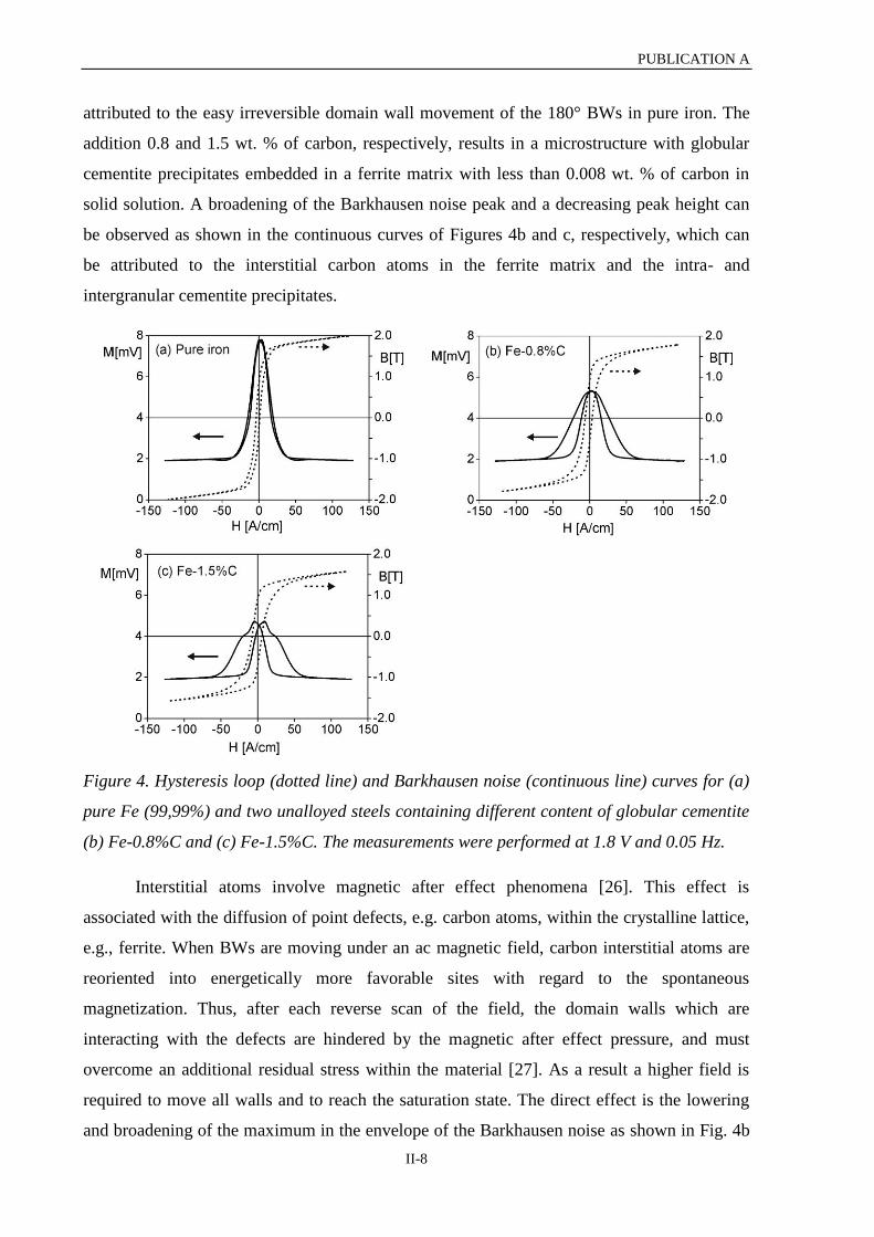
PUBLICATION A
II-8
attributed to the easy irreversible domain wall movement of the 180° BWs in pure iron. The
addition 0.8 and 1.5 wt. % of carbon, respectively, results in a microstructure with globular
cementite precipitates embedded in a ferrite matrix with less than 0.008 wt. % of carbon in
solid solution. A broadening of the Barkhausen noise peak and a decreasing peak height can
be observed as shown in the continuous curves of Figures 4b and c, respectively, which can
be attributed to the interstitial carbon atoms in the ferrite matrix and the intra- and
intergranular cementite precipitates.
Figure 4. Hysteresis loop (dotted line) and Barkhausen noise (continuous line) curves for (a)
pure Fe (99,99%) and two unalloyed steels containing different content of globular cementite
(b) Fe-0.8%C and (c) Fe-1.5%C. The measurements were performed at 1.8 V and 0.05 Hz.
Interstitial atoms involve magnetic after effect phenomena [26]. This effect is
associated with the diffusion of point defects, e.g. carbon atoms, within the crystalline lattice,
e.g., ferrite. When BWs are moving under an ac magnetic field, carbon interstitial atoms are
reoriented into energetically more favorable sites with regard to the spontaneous
magnetization. Thus, after each reverse scan of the field, the domain walls which are
interacting with the defects are hindered by the magnetic after effect pressure, and must
overcome an additional residual stress within the material [27]. As a result a higher field is
required to move all walls and to reach the saturation state. The direct effect is the lowering
and broadening of the maximum in the envelope of the Barkhausen noise as shown in Fig. 4b
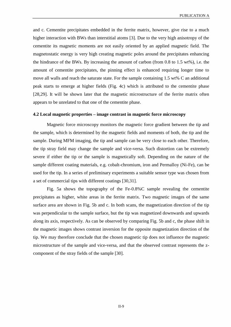
PUBLICATION A
II-9
and c. Cementite precipitates embedded in the ferrite matrix, however, give rise to a much
higher interaction with BWs than interstitial atoms [3]. Due to the very high anisotropy of the
cementite its magnetic moments are not easily oriented by an applied magnetic field. The
magnetostatic energy is very high creating magnetic poles around the precipitates enhancing
the hindrance of the BWs. By increasing the amount of carbon (from 0.8 to 1.5 wt%), i.e. the
amount of cementite precipitates, the pinning effect is enhanced requiring longer time to
move all walls and reach the saturate state. For the sample containing 1.5 wt% C an additional
peak starts to emerge at higher fields (Fig. 4c) which is attributed to the cementite phase
[28,29]. It will be shown later that the magnetic microstructure of the ferrite matrix often
appears to be unrelated to that one of the cementite phase.
4.2 Local magnetic properties – image contrast in magnetic force microscopy
Magnetic force microscopy monitors the magnetic force gradient between the tip and
the sample, which is determined by the magnetic fields and moments of both, the tip and the
sample. During MFM imaging, the tip and sample can be very close to each other. Therefore,
the tip stray field may change the sample and vice-versa. Such distortion can be extremely
severe if either the tip or the sample is magnetically soft. Depending on the nature of the
sample different coating materials, e.g. cobalt-chromium, iron and Permalloy (Ni-Fe), can be
used for the tip. In a series of preliminary experiments a suitable sensor type was chosen from
a set of commercial tips with different coatings [30,31].
Fig. 5a shows the topography of the Fe-0.8%C sample revealing the cementite
precipitates as higher, white areas in the ferrite matrix. Two magnetic images of the same
surface area are shown in Fig. 5b and c. In both scans, the magnetization direction of the tip
was perpendicular to the sample surface, but the tip was magnetized downwards and upwards
along its axis, respectively. As can be observed by comparing Fig. 5b and c, the phase shift in
the magnetic images shows contrast inversion for the opposite magnetization direction of the
tip. We may therefore conclude that the chosen magnetic tip does not influence the magnetic
microstructure of the sample and vice-versa, and that the observed contrast represents the z-
component of the stray fields of the sample [30].

PUBLICATION A
II-10
Figure 5. Topography (a) of the sample Fe-0.8%C containing globular cementite precipitates
in a ferrite matrix, MFM images taken with the magnetic tip magnetized downwards (b) and
upwards (c) along its axis [29].
4.3 MFM images of high purity iron
Fig. 6a-c demonstrate the evolution of the magnetic microstructure for the high purity
iron sample in an external in-plane magnetic field. Fig. 6a shows the sample at the remanence
state (no applied field) while Fig. 6b and c show the sample in an applied magnetic field of
190 A/cm and -190 A/cm, respectively. Arrow #1 in Fig. 6a points to a grain boundary
separating two grains with different crystal orientation. The grain on the right side displays a
multitude of small areas with different magnetic contrast, while the grain on the left side
shows large areas with almost homogeneous grey level. The domain arrangement at the
surface is primarily determined by the principle of flux closure which minimizes the total
inner energy. Besides that, it is strongly dependent on the surface orientation relative to the
easy directions. From the simplest case, a surface containing two easy axes, to surfaces
strongly deviating from easy axes in their orientation, the domain patterns become
progressively more and more complicated [14]. The <001> directions are the easy directions
for iron and therefore the (100) surface contains two mutually perpendicular easy directions.
This allows us to conclude that the orientation of the left grain is close to the plane (100), and

PUBLICATION A
II-11
the orientation of the right grain strongly deviates from the plane (100), which contains two
easy axes.
The grain on the left side displays a few domains clearly separated by Bloch walls
which can be detected as bright or dark lines in the MFM image (arrows #2 and #3) in Fig. 6).
At the remanence state, a domain wall will be in a position which minimizes the energy of the
system formed by the wall itself and the adjoining domains and domain walls. In Fig. 6a,
some walls are bulged possibly indicating the existence of defects and residual microstress
which is caused by crystal imperfections as e.g. dislocations [18].
When the magnetic field is applied a change of position of the domain can be
observed. For example a small domain wall indicated by arrow #3 in Fig. 6 moves to the right
or left side when a positive or negative field is applied, respectively. In order to highlight the
domain wall movements, the arrows were placed in exactly the same positions in all images
by taking the immobile grain boundary (arrow #1) as a reference. All domain walls go back to
their initial positions when the field is switched off, which means that the observed domain
wall movements are reversible.
Figure 6. MFM images of the high purity iron sample (a) without external field and with an
applied external field of (b) 190 A/cm and (c) – 190 A/cm, respectively. The direction of the
in-plane field is indicated by black arrows.
4.4 MFM images of the samples containing globular cementite embedded in a ferrite
matrix
Non-magnetic inclusions in a magnetic matrix are often discussed in literature [32,33],
in contrast the unalloyed steels Fe-0.8%C and Fe-1.5%C investigated here consist of a soft
ferromagnetic ferrite matrix with cementite precipitates which are magnetically harder than
the matrix. The carbon content is higher in the Fe-1.5%C sample than in the

PUBLICATION A
II-12
Fe-0.8%C-sample, but the basic behavior of the magnetic microstructure can be discussed by
taking the Fe-1.5%C as an example.
Fig. 7 shows the microstructure of the Fe-1.5%C sample. The topography image
obtained with the MFM (Fig. 7a) reveals the cementite precipitates as bright areas which are
about 400 nm at maximum higher than the ferrite matrix. Three grains with different average
height (numbered (1), (2), and (3)) are visible in the ferrite matrix. The corresponding electron
backscatter diffraction maps taken with a scanning electron microscope, i.e. the Kikuchi
pattern quality (KPQ) and the inverse pole figure (IPF), are shown in Fig. 7b and c,
respectively. The color code of the inverse pole figure represents the crystallographic
orientation in the ferrite matrix (nearly pure b.c.c. iron, lattice constant a = 2.87Å), and in the
cementite particles (orthorhombic symmetry, length of the three perpendicular axes a =
5.09Å, b = 6.74Å, c = 4.52Å). Using an orientation imaging software the angles of inclination
of the three ferrite grains (1), (2), and (3) relative to the (100) plane were obtained as 15°, 9°
and 33°, respectively.
The inverse pole figure maps reveal that most of the large cementite precipitates
observed in the topography image (Fig. 7a) are not single crystals, but have a polycrystalline
structure with different grain orientations. The dark grey color of the cementite precipitates in
the KPQ map corresponds to a low KPQ index (Fig. 7b). The decrease of the indexing rate is
correlated with a strong lattice distortion induced by accumulation of dislocations in the
cementite phase.
Fig. 8a-d displays the magnetic microstructure of the same sample area shown in Fig.
7 in the demagnetized state as well as with applied field strengths of 100 and 190 A/cm,
respectively. Like in the Fe-0.8%C sample (Fig. 5), the cementite precipitates show mostly
striped domains with a strong magnetic phase contrast, while the contrast in the ferrite matrix
is weaker. This can be explained by the fact that cementite is magnetically harder than ferrite
and thus causes stronger stray fields. Each cementite particle has its own domain structure,
and no closure domains are observed. This probably is due to the high single crystal
anisotropy of cementite (K1 = 118.103 J.m
-3 and K2 = 394.10
3 J.m
-3) [7]. The cementite
domain structure in or around the (010) plane consists of parallel stripes directed alternately
down- and upwards in relation to the surface. Since the MFM tip senses the component of the
stray field emerging perpendicularly from the surface, we may conclude that the magnetic
moments of these precipitates are more or less parallel to the tip axis, i.e. perpendicular to the
sample surface plane. The observation that the long axis (here [010]- or b-axis) is the easy

PUBLICATION A
II-13
axis in cementite agrees with the results of Keh and Johnson, obtained by transmission
electron microscopy studies on cementite particles with 5-10 µm average dimension [7].
Figure 7. Topography (a) of the Fe-1.5%C sample taken with MFM. The corresponding KPQ
(b) and IPF (c) maps taken with SEM show the crystals and their respective orientations.
Three grains with different crystal orientation are marked as (1), (2), and (3) in the images.
Spike domains, first observed by Williams [42] in a Fe-Si alloy, are visible in the
ferrite matrix on the grain boundary between the grains 1 and 3 as well as attached to the large
precipitate (white arrow (S) in Fig. 8a). The formation of these spike domains may be
explained by the reduction of the magnetostatic energy of the cementite and stress
concentrations on the grain boundary and on the cementite/ferrite interface caused by
differences in thermal expansion coefficient. Magnetostatic energy associated with an
inclusion is proportional to its volume. Thus the probability to show attached spike domains
in order to reduce magnetostatic energy increases with the size of the precipitates.
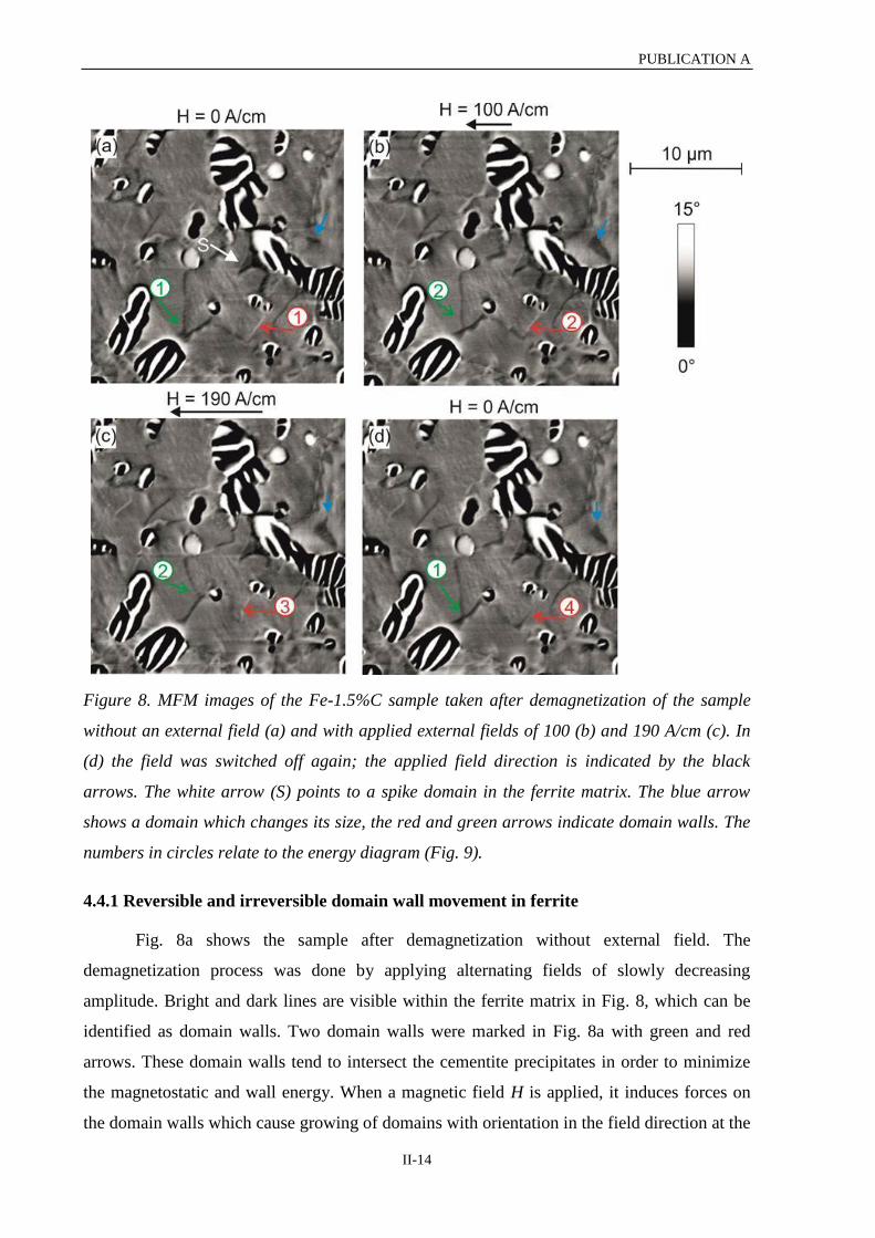
PUBLICATION A
II-14
Figure 8. MFM images of the Fe-1.5%C sample taken after demagnetization of the sample
without an external field (a) and with applied external fields of 100 (b) and 190 A/cm (c). In
(d) the field was switched off again; the applied field direction is indicated by the black
arrows. The white arrow (S) points to a spike domain in the ferrite matrix. The blue arrow
shows a domain which changes its size, the red and green arrows indicate domain walls. The
numbers in circles relate to the energy diagram (Fig. 9).
4.4.1 Reversible and irreversible domain wall movement in ferrite
Fig. 8a shows the sample after demagnetization without external field. The
demagnetization process was done by applying alternating fields of slowly decreasing
amplitude. Bright and dark lines are visible within the ferrite matrix in Fig. 8, which can be
identified as domain walls. Two domain walls were marked in Fig. 8a with green and red
arrows. These domain walls tend to intersect the cementite precipitates in order to minimize
the magnetostatic and wall energy. When a magnetic field H is applied, it induces forces on
the domain walls which cause growing of domains with orientation in the field direction at the

PUBLICATION A
II-15
expense of the other domains. A supplementary domain can be observed in grain 2 (Fig. 8,
blue arrows). When applying a field of 100 and 190 A/cm (Fig. 8b and c) respectively, the
domain increases its size. When the magnetic field is switched off, the size of the domain
decreases again (Fig. 8d).
At low fields, domain wall motion dominates the magnetization process rather than
domain rotation. However, both domain wall bulging (a reversible process) and domain wall
displacement (an irreversible process) are important in this region. Initially, if the magnetic
field is smaller than the coercive field (H < Hc), the domain wall is attached to pinning points.
As H increases, the wall bows between the pins as to be seen in Fig. 8b, red arrow. When H >
Hc, the domain wall unpins and propagates (Fig. 8c, red arrow).
In order to explain such a displacement as observed by the domain wall marked by red
arrows in Fig. 8, one can use a well-known model (Fig. 9) [18]. The domain wall
displacement x can be described as a function of a single energy term E which stands for all
types of energies involved such as wall energy and magnetostatic energy. The energy E varies
with x as shown schematically in Fig. 9a. The magnetic field H causes a driving force on the
domain wall which acts against the restoring force of energy gradient dE/dx (Fig. 9b). One
can assume that the driving force is cH, where the proportionality constant c depends on the
kind of wall and on the orientation of the field. At H = 0, the wall “rests” in an energy
minimum (upon a cementite precipitate) (Figs. 8a and 9). If a small field is applied, with cH
lower than the maximum of the energy gradient, the wall moves reversibly to point and
back to point , if H is switched off again (Figs. 8d and 9). If a larger field H is applied
such that cH is equal or larger to the maximum of the energy gradient, the wall jumps
irreversibly to point (Figs. 8c and 9). If H is now switched off again, the wall will move
to point , which then is the nearest minimum in energy (Figs. 8d and 9). Note that for the
same external applied in-plane magnetic field both reversible (green arrows in Fig. 8) and
irreversible (red arrows in Fig. 8) domain wall movements are observable, because the shape
and the gradient of the energy curve in Fig. 9 depend on the domain wall and on its
microstructural neighborhood.

PUBLICATION A
II-16
Figure 9. Energy model for reversible and irreversible domain wall movements in x-direction.
The external force on the domain wall acting against the internal force dE/dx is proportional
to the applied external field H. The wall will move back from to the energy minimum as
long as cH is smaller than the local maximum of dE/dx. If cH is equal or larger than the
maximum, the wall will jump from ’ to and back to a new minimum upon removal of
the external field.
It is clearly visible that the magnetic microstructure of ferrite and the evolution of its
domain configuration under an applied magnetic field are strongly influenced by the
cementite. Domain walls are hindered in their movement by large as well as by small
precipitates. For large precipitates, this is mainly due to interactions with attached subsidiary
domains which tend to stick to the walls, whereas small precipitates reduce the energy of any
wall that contains them. In relation to their volume density, inclusions with a diameter
approximately equal to the wall thickness should cause the strongest effect [18]. The pinning
sites cause a decrease in the initial permeability of a ferromagnetic material and an increase in
its coercive force. Hence, increasing the amount of carbon, i.e. cementite, the macroscopic
initial permeability decreases and the coercivity increases. Irreversible changes in
magnetization are caused during wall displacement by the pinning process [35]. A wall jump
generates an eddy current pulse which propagates in all directions and arrives at the surface of
the sample according to a dispersion law [43]. The average of all local Barkhausen jumps can
be detected by a suitable macroscopic set-up as shown in Fig. 1.

PUBLICATION A
II-17
Fig. 10 shows the evolution of the magnetic microstructure of a section of grain (1) in
Fig. 7. The magnetic microstructure is slightly different from the structure in Fig. 8 because
the sample was removed from the MFM, demagnetized in a strong macroscopic field, and
replaced into the MFM between the measurements. Fig. 10a is recorded at the remanence
state of the sample while Fig. 10b and c display the results with an applied magnetic field of
190 A/cm and -190 A/cm, respectively. The walls (arrows in Fig. 10) are anchored at the
precipitates. Fig. 10a (arrow #1) shows a wall which is already bent between two cementite
precipitates without an applied external field. When applying a field of 190 A/cm to the right
(Fig. 10c) the wall becomes nearly straight. Contrarily, the wall marked with arrow #2 is
nearly straight when no external field is applied (Fig. 10a), but it clearly bends into the
direction of the field of 190 A/cm (Fig. 10c). This confirms the predictions [34] that domain
walls should be flexible rather than rigid. An irreversible domain wall movement (Barkhausen
jump) is also visible as marked by arrow #3 in Fig. 10a-c. One Bloch wall shows a sharp kink
(Fig. 10c, arrow K). The kink in a 180° Bloch wall has also been observed in magnetite using
the Bitter method [5]. Bloch wall segments with different polarities do not form a straight
line, but are kinked at the point where the direction of the interior rotation of spins in the wall
reverses. This reduces the magnetostatic (stray field) energy of the wall.
Figure 10. MFM images taken on the Fe-1.5%C sample (a) without external field and with
external fields of (b) 190 A/cm and (c) – 190 A/cm, respectively. The applied field direction is
indicated by the black arrows [29].
4.4.2 Bowing of domain walls in ferrite
Residual stresses in the ferrite phase as well as lattice mismatch in both phases may
produce microstresses, which can cause bowing of 180° walls even without applied field.

PUBLICATION A
II-18
Fig. 11a shows a sketch of a 180° Bloch wall which is bowed into a circular arc of radius r.
The dotted line gives the position of the unflexed wall; 2y is the distance between pinning
sites and x the linear displacement [35]. The linear displacement x is obtained by a simple
geometrical calculation (Fig. 11a):
√ . (3)
The average internal stress <> responsible for the observed domain wall bowing can be
estimated as [36]:
( ⁄ )
(
⁄ ). (4)
Here, s = 22.2 10-6
is the saturation magnetostriction constant for iron [100] [19],
0 = 1.256 10-6
N/A2 is the magnetic permeability in vacuum, and
Ms = 1.739 106 A/m [19] is the saturation magnetization of iron. Taking the measured
values r = 48.1 m, x = 0.1 m and y = 3.1 m, the estimated value of the average internal
stress is <> = 88.9 MPa (Fig. 11b, white arrow).
Figure 11. Bending of a magnetic domain wall between two pinning sites: (a) schematic
sketch showing the geometry of the curved domain wall [37], (b) and (c) enlarged section of
Fig. 10 showing the Fe-1.5%C sample at the remanence state and with an applied field of 190
A/cm to the right, respectively.
The amount of domain wall bending before breaking away from the pinning sites
depends directly (but inversely) on the strength of the pinning sites and on the domain wall
surface energy [35]. The domain wall undergoes more bending for a wall having low surface

PUBLICATION A
II-19
energy and high pinning site strength. Furthermore the bending depends on an extrinsic factor
which depends on the magnetic field H.
4.4.3 Contrast and width of domain walls in ferrite
Bloch walls in the ferrite matrix are visible as bright and dark lines in the scanned
area. Fig. 12 shows once more an enlarged section of an MFM image of grain 1. MFM line
scans across both walls are shown in Fig. 12b and c. The line scans clearly show the positive
and negative phase shifts in the bright and dark walls, respectively. For a wall moment
direction opposite to the tip moment direction, the tip will feel a repulsive force and the
cantilever suffers a positive phase shift resulting in a bright line in the image. Vice versa, for a
magnetic moment direction in the wall parallel to the moment of the tip, it will feel an
attractive force creating a negative phase shift and a dark line in the image. The average
magnetic moments inside the walls are perpendicular to the plane pointing out of or into it.
We can conclude that on both sides of a wall, the magnetic moments are most likely
antiparallel to each other and aligned in the plane. The BWs are transition areas in which the
moment direction gradually rotates by 180°. As a consequence, the MFM tip feels an
attractive or a repulsive force on the walls depending on their polarities.
Depending on the magnetic anisotropy value, the domain wall width δw can vary from
a few inter-atomic distances in hard magnetic films with perpendicular anisotropy to several
hundred nanometers in films with weak in-plane anisotropy [38]. The width of a BW in iron
is around 100 nm [39,40]. In this work, the wall width measured in the ferrite phase ranges
from 140 nm to about 500 nm. The larger value found in this work can be explained by
limited local resolution of the MFM instrument caused by the finite horizontal and vertical
dimensions of the tip apex and corresponding averaging over the local stray-field variation
[41].

PUBLICATION A
II-20
Figure 12. (a) Enlarged section of Fig. 10a showing Bloch walls in the Fe-1.5%C sample; (b)
and (c) line scans across the Bloch walls, lines indicated in (a). The measured wall thickness
in the line scans (1) and (2) is 500 nm and 340 nm, respectively.
4.5 Correlation between microscopic and macroscopic magnetic measurements
With increasing amount of cementite in the ferrite matrix the macroscopic magnetic
hardness increases. As has been shown in sections 4.2, 4.3, and 4.4, the domain structure of
the pure iron sample is completely different from the domain structure of the material with the
cementite phase. The cementite particles show a magnetic stray field which is in generally
stronger than the stray field of the ferrite, and the magnetic microstructure of ferrite is
strongly influenced by the cementite. An interaction between the domain walls in ferrite with
the precipitates becomes very well visible when an external magnetic field is applied.
Observation of the position change of the domain walls at different external magnetic fields
indicated clearly that the domain walls of the ferrite matrix are hindered in their movement by
large as well as by small cementite precipitates.
The analysis of the magnetic microstructure of the investigated samples suggests that
the field of 190 A/cm is not strong enough to reach saturation. However, the macroscopic
measurements have shown that a field of 190 A/cm is strong enough to saturate all three
samples. This disagreement may be explained by the fact that the macroscopic hysteresis loop
measurements were made with cylindrical samples while the samples for MFM measurements
were small square plates cut from the macroscopic cylinders. Shape anisotropy and
demagnetization probably led to different magnetic fields in the completely different
experimental geometries. Furthermore the MFM analysis of the domains and their dynamics
relies on the behavior of the surface domains. Surface residual stress built up during
mechanical polishing as well as the special electromagnetic boundary conditions of surface
domains may hinder the movement of domain walls on the surface and thus a stronger

PUBLICATION A
II-21
magnetic field may be required to reach the same magnetization level compared to the volume
interior.
5. SUMMARY
Samples of highly pure iron and the unalloyed steels Fe-0.8%C and Fe-1.5%C were
characterized macroscopically by measuring hysteresis loops and Barkhausen noise signals.
With increasing amount of carbon in form of globular cementite precipitates in the ferrite
matrix the magnetic hardness increases and the Barkhausen noise amplitude decreases.
The local resolution of most magnetic imaging techniques is not sufficient to observe
individual domains in technical steels. Interpretations therefore are based on simulation,
macroscopic experiments and on observations in materials with a coarser micro structure. The
combination of AFM, MFM, and EBSD techniques opens a new field for material research
and development enabling the direct observation of magnetic micro- and nanostructures
including the corresponding single crystal grain orientations. The surface of bulk samples can
be studied, the comparison to macroscopic data of the samples is therefore possible, and the
sample preparation is simpler compared to sample preparation for transmission electron
microscopy.
In this work, MFM images with a local resolution of 50 nm, recorded with different
external fields reveal how the magnetization process takes place via domain wall
displacement and domain wall nucleation. Ferromagnetic domain structures in highly pure
iron and in cementite precipitates as well as their interaction were studied. Domain walls in
the ferrite phase tend to intersect the cementite precipitates in order to minimize the
magnetostatic and wall energy. Spike domains have been observed mostly in the grain
boundaries of the ferrite phase as well as attached to large cementite precipitates. The
cementite domain structure in or around the (010) plane was found to consist of parallel
stripes directed alternately down- and upwards in relation to the surface without direct
correlation to the ferrite domain structure of the matrix.
By applying an external in-plane magnetic field the dynamic behavior of the magnetic
domains and the interaction between domain walls and the cementite precipitates was
observed. In the ferrite matrix, bending of domain walls occurs at weak external magnetic
fields. For stronger applied magnetic fields reversible and irreversible break-free of domain
walls was observed, which can be interpreted as a local Barkhausen event or -jump. The
microscopic observation that the cementite precipitates represent an obstacle to the domain
wall movement correlates qualitatively with the increase of magnetic hardness with increasing

PUBLICATION A
II-22
amount cementite, and with the broadening of the maximum in the envelope of the
Barkhausen noise in the macroscopic measurements.
REFERENCES
[1] I. Altpeter, Journal of Nondestructive Evaluation 15 (1996) 45.
[2] I. Altpeter, G. Dobmann, M. Kröning, M. Rabung, S. Szielasko, NDT&E International 42
(2009) 283.
[3] C. Gatelier-Rothea, J. Chicois, R. Fougeres, P. Fleischmann, Acta Materialia 46 (1998)
4873.
[4] S.M. Thompson, B.K. Tanner, Journal of Magnetism and Magnetic Materials 123 (1993)
283.
[5] Ö. Özdemir, D.J. Dunlop, Journal of Geophysical Research 102 (1997) 20,211.
[6] R. Schäfer, Journal of Magnetism and Magnetic Materials, 215-216 (2000) 652.
[7] A. S. Keh, C. A. Johnson, Journal of Applied Physics 34 (1963) 2670.
[8] I. Manke, N. Kardjilov, R. Schäfer, A. Hilger, M. Strobl, M. Dawson, C. Grünzweig, G.
Behr, M. Hentschel, C. David, A. Kupsch, A. Lange, J. Banhart, Nature Communications 1
(2010) 125.
[9] P. Grütter, T. Jung, H. Heinzelmann, A. Wadas, E. Meyer, H.R. Hidberand, H.J.
Güntherodt, Journal of Applied Physics 67 (1990) 1437.
[10] U. Hartmann, Journal of Magnetism and Magnetic Materials, Volumes 157–158 (1996)
545.
[11] E. Dan Dahlberg, Jian-Gang Zhu, Physics Today 48 (1995) 34.
[12] U. Hartmann, T. Göddenhenrich, C. Heiden, Journal of Magnetism and Magnetic
Materials, 101 (1991) 263.
[13] P. Grütter, H. J. Mamin, D. Rugar, in Scanning Tunneling Microscopy, Vol. II, ed. by
H.J. Güntherodt, R. Wiesendanger, Springer, Berlin, Heidelberg, New York (1992) 845.
[14] A. Hubert, R. Schäfer, Magnetic Domains - The Analysis of Magnetic Microstructures,
Springer, Berlin (1998).
[15] H. Kronmüller, S. Parkin, Handbook of Magnetism and Advanced Magnetic Materials,
Vol 2: Micromagnetism, Wiley & Sons, New York (2007).
[16] M. Coisson, F. Vinai, P. Tiberto, F. Celegato, Journal of Magnetism and Magnetic
Materials 321 (2009) 806.
[17] S. Huo, J. E. L. Bishop, J. W. Tucker, M. A. Al-Khafaji, W. M. Rainforth, H. A. Davies,
M. R. J. Gibbs, Journal of Magnetism and Magnetic Materials 190 (1998) 17.

PUBLICATION A
II-23
[18] B. D. Cullity, Introduction to magnetic materials, Addison Wesley, London (1972).
[19] H. Kronmüller, M. Fähnle, Micromagnetism and the Microstructure of Ferromagnetic
Solids, Cambridge University Press, Cambridge (2003).
[20] E. Kneller, Ferromagnetismus, Springer, Berlin (1962).
[21] Y. Martin, H.K. Wickramasinghe, Applied Physics Letters 50 (1987) 1455.
[22] J.J. Saenz, N. Garcia, P. Griitter, E. Meyer, H. Heinzelmann, R. Wiesendanger, L.
Rosenthaler, H.R. Hidber, H.J. Güntherodt, Journal of Applied Physics 62 (1987) 4293.
[23] G. Binning, C.F. Quate, C. Gerber, Physical Review Letters 56 (1986) 930.
[24] Q. Zhong, D. Inniss, K. Kjoller, V.B. Elings, Surface Science, 290 (1993) L688.
[25] A. Thiaville, J. Miltat, J. M. García, Magnetic Force Microscopy: Images of
Nanostructures and Contrast Modeling, in: NanoScience and Technology, No. XVIII, Eds. H.
Hopster, H. P. Oepen, Springer Berlin Heidelberg (2005) 128.
[26] P. Brissonneau, Journal of Physics and Chemistry of Solids 7 (1958) 22.
[27] J. M. Lopez, Caractérisation de la précipitation du carbone dans les alliages Fe–C par
des mesures magnétiques et magnétomécaniques, Thèse, Université P. Sabatier, Toulouse
(1986).
[28] G. Dobmann, private communication.
[29] I. Altpeter, Spannungsmessung und Zementitgehaltsbestimmung in Eisenwerkstoffen
mittels dynamischer magnetischer und magnetoelastischer Meßgrößen, Dissertation, Saarland
University, Saarbrücken (1990).
[30] S. Wust, Untersuchung der magnetischen Domänen in Stahlproben mittels
Magnetkraftmikroskopie unter Anlegen eines externen Magnetfeldes, Diploma thesis,
Saarland University, IZFP report No.110126-TW, Saarbrücken (2011).
[31] L. Batista, U. Rabe, S. Hirsekorn, "Micro- and Nanostructure Imaging and
Characterization of Advanced Steels", 38th Annual Review of Progress in Quantitative
Nondestructive Evaluation (QNDE), July 17-22, 2011, Burlington, Vermont, USA.
[32] L. Néel, Cahiers de Physique 25 (1944) 21.
[33] M. Kersten, Grundlagen einer Theorie der ferromagnetischen Hysterese und der
Koerzitivkraft, S. Hirzel, Leipzig (1943).
[34] M. Kersten, Zeitschrift für Angewandte Physik 7 (1956) 313.
[35] D. C. Jiles, D.L. Atherton, Journal of Magnetism and Magnetic Materials 61 (1986) 48.
[36] S. Xu, R.T. Merril, Journal of Geophysical Research, 97 (1992) 4321.
[37] A. Globus, P. Duplex, M. Guyot, IEEE Transactions on Magnetics MAG-7 (1971) 617.
[38] V. Zablotskii, J. Ferré, A. Maziewski, Journal of Physics D: Applied Physics 42 (2009).

PUBLICATION A
II-24
[39] A.E. Berkowitz, E. Kneller, Magnetism and Metallurgy, Vol. 1, Academic Press New
York, London (1969).
[40] C. Kittel, Review of Modern Physics, 21 (1949) 541.
[41] U. Hartmann, Annual Review of Materials Science 29 (1999) 53.
[42] H. J. Williams, Physical Review 71 (1947) 646.
[43] G. Dobmann, “NDT – Do we have the potential to predict material properties as yield
strength, tensile strength and fracture toughness on the component? A state of the art survey”,
18th European Conference on Fracture, Dresden, 30.08.-03.09.2010.

II-25


PUBLICATION B
III-1
III. ON THE MECHANISM OF NONDESTRUCTIVE EVALUATION OF
CEMENTITE CONTENT IN STEELS USING A COMBINATION OF
MAGNETIC BARKHAUSEN NOISE AND MAGNETIC FORCE
MICROSCOPY TECHNIQUES (PUBLICATION B)
L. Batista, U. Rabe, I. Altpeter, S. Hirsekorn, and G. Dobmann
Journal of Magnetism and Magnetic Materials (2014) Vol. 354; 248-256.
ABSTRACT. The influence of the carbon content in form of globular cementite precipitates
in unalloyed steels was macroscopically characterized by means of magnetic hysteresis loop
and Barkhausen noise techniques. The choice of the frequency of the applied field has a
strong influence on the Barkhausen noise profiles. At sufficiently high frequency (0.5 Hz)
there are two peaks, one at lower field, the amplitude of which corresponds to the amount of
ferrite and one at higher field, the amplitude of which corresponds to the amount of the
cementite phase, respectively. Magnetic force microscopy and electron backscattered
diffraction techniques were used to determine the magnetic and crystallographic
microstructures of the steels. Cementite has its own domain structure and stray fields which
influence the magnetization process of the steel by its own magnetic contribution. When an
external magnetic field is applied, the magnetization process in ferrite occurs mainly at lower
fields through the 180° and 90° domain walls. A higher field is required for the observation of
180° domain wall movements in cementite.
Keywords: Magnetic force microscopy (MFM), Electron backscatter diffraction (EBSD),
Steel, Magnetic domains, Barkhausen noise, Non-destructive testing

PUBLICATION B
III-2
1. INTRODUCTION
In most steels, among all the phases or constituents that can be obtained by choosing
the chemical composition and thermo-mechanical treatments, two are frequently encountered:
ferrite and cementite. Ferrite shows high ductility and low strength values and therefore low
mechanical and also - very often - magnetic hardness in terms of coercivity. Cementite on the
other hand shows high mechanical and magnetic hardness and is much more brittle. Thus, the
relative volume fraction of the ferrite and cementite phases gives rise to the final mechanical
and magnetic properties of the steel. The knowledge of the amount of cementite in steels is
thus crucial.
Hysteresis loop and magnetic Barkhausen noise (MBN) evaluations are widely used
magnetic measurement techniques for the microstructural characterization of ferromagnetic
materials and determination of residual stress states. In physics, regular hysteresis
measurements providing reproducible and reliable results can only be performed by using
special hystrometer measurement devices asking for specially shaped test specimens like
spheres and cylinders with well-designed geometry combined with encircling coils to measure
the magnetic induction. As a consequence the technique can not be applied to real
components, as for instance vessel shells or pipes or high speed running steel sheets in a cold
rolling mill [1], and is therefore destructive. All techniques based on magnetic circuit
approaches [2] suffer from influence of lift-off on absolute value, ensuing value fluctuations,
and shearing of the hysteresis curve [3]. Only in case of transformer steel sheets industrial
consensus standards exist (i.e. Epstein frame measurements [4]) based on destructive batch
tests. In contrast to these facts MBN-analysis can be performed with sensors positioned
locally on top of the surface of a component, which means that MBN is non-destructive.
However, the use of the magnetic Barkhausen noise techniques is “not yet” regulated by a
standard. This makes the comparison of results published by different authors extremely
difficult, especially as the side influences of different experimental conditions such as
magnetization set-up, signal pick-up, band width, etc. are often insufficiently described. First
attempts into standardization are initialized by the German Engineering Society (VDE
Guidelines) [5].
During the magnetization process the domain structure of a ferromagnetic material is
altered which involves different movements of the domain walls. There are exclusively 90°-
and 180°- domain walls in case of iron materials. In the case considered here, the domain wall
movement takes place in a microstructure consisting of a ferrite matrix with cementite
precipitates. In basic physics the precipitates are either assumed acting as nonmagnetic
PUBLICATION B
III-3
foreign bodies [6,7] in the ferromagnetic matrix, or they are considered to interact with the
domain walls of the matrix via their residual stress fields [8]. Domain walls tend to cling to
nonmagnetic inclusions in order to minimize the magnetostatic and the wall energy. It was
considered in the literature in a first approach that cementite behaves as a nonmagnetic
inclusion in a ferrite matrix [9] or even as a nonmagnetic phase at all [10]. However,
cementite is a ferromagnetic phase [11,12], and therefore – depending on its size, shape,
crystalline orientation and amount of defects - it has its own domain structure and stray fields.
The stray fields of inclusions, which are a source of magnetostatic energy, may also interact
with the domain walls within the matrix. In order to reduce the magnetostatic energy,
supplementary domains (closure domains) are built close to the inclusions which in turn
interact with the domain walls in the matrix [13,14]. The other source of interaction of the
cementite precipitates with the domain walls in the ferrite phase are – as mentioned above -
the residual stresses which are built-up due to different thermal expansion coefficients of the
two phases during the solidification process of the material, and lattice defects, e.g.
dislocations, which are created on the interface between ferrite and cementite.
Several studies have been done on the individual influence of different microstructural
parameters, e.g. second phase particles, on the generation of the magnetic Barkhausen noise.
For example, the observed MBN activity profile in a microstructure containing cementite in a
ferrite matrix showed either a single [15] or a double peak [8,16]. The description of a double
peak for a Barkhausen noise profile has also encountered divergences in the literature. The
weaker field peak was attributed to the pinning of 180° walls in the matrix by secondary
particles and the stronger field peak was explained by annihilation of 90° domain walls at
grain boundaries [17]. Contrarily, Moorthy et al. [16] stated that the weaker field peak is
caused by irreversible domain walls in the ferrite and the stronger field peak by irreversible
movement of domain walls overcoming second phase particles. By measuring the MBN
signal as a function of temperature of a compact cementite and unalloyed white cast iron
samples, Altpeter [18] demonstrated that the cementite actively produces its own MBN signal.
With increasing temperature the ferromagnetic coordination decreases, and consequently the
MBN signal intensity decreases. The Curie temperature of cementite (~ 210°C) is lower than
the Curie temperature of ferrite ( 770°C). Altpeter observed a Barkhausen noise amplitude of
the compact cementite specimen, which decreased with increasing temperature and
disappeared at the Curie temperature of cementite [18]. Furthermore, the MBN amplitude of
white cast iron showed qualitatively the same behavior, i.e. it decreased strongly towards the
Curie temperature of cementite and remained at a low almost constant level above this value.

PUBLICATION B
III-4
In addition, the MBN decrease of white cast iron was stronger with increasing amount of
cementite.
In this work, we investigate the opportunity of assessing the relative proportion and
contributions of the cementite and ferrite phases in unalloyed steels by optimizing the
measured hysteresis loop and Barkhausen noise parameters. The evolution of the magnetic
microstructure is directly correlated to the macroscopic measurement quantities by means of a
superposed magnetic field applied to a magnetic force microscope (MFM).
2. MATERIALS AND METHODS
Three different materials were examined in this study, a high purity iron (99.99%) and
two unalloyed steels, Fe-0.8%C and Fe-1.5%C, containing globular cementite (Fe3C)
embedded in a ferrite matrix. The samples were provided as-cast and machined in a
cylindrical shape of 8 mm diameter and 50 mm length. In order to remove all processing-
induced residual stresses the samples were vacuum annealed at 600°C for 4h. The resulting
microstructure has an average grain size of 80 m for all samples. The size of the cementite
precipitates ranges from a few hundred nanometers to about 10 m in diameter.
The hysteresis loop and Barkhausen noise measurements were performed inside an
electromagnet with a computer-controlled bipolar power supply (Fig. 1). The magnetic
tangential field strength H was measured by a Hall probe. The cylindrical samples were
magnetized along their axial direction up to a maximum magnetic field strength of 11000 A/m
at different excitation frequencies of 0.05 Hz, 0.1 Hz and 0.5 Hz, respectively. The change in
magnetic flux density B and the magnetic Barkhausen noise amplitude M were measured by a
pick-up coil with 300 turns (wire diameter: 0.1 mm, resonance frequency: 710 kHz)
surrounding the sample (Fig. 1). The envelope of the noise signals (analyzed frequency range
fA = 200 Hz - 50 kHz) and the magnetic flux density were recorded as a function of the
tangential field strength.

PUBLICATION B
III-5
Figure 1. (a) Schematic sketch of the experimental set-up for hysteresis loop and Barkhausen
noise measurements, (b) schematic hysteresis loop with coercive field HC, magnetic flux at
saturation BS, remnant magnetic flux BR, and loss per cycle W, (c) schematic Barkhausen
noise curve with maximum amplitudes Mmax1,2, remnant Barkhausen noise amplitude MR, and
coercive field Hcm1,2 deduced from Barkhausen noise curve.
Small specimens (3 x 3 x 1 mm3) were cut by spark erosion from the annealed
cylindrical samples for the atomic force microscopy (AFM) and magnetic force microscopy
investigations. The specimens were mechanically polished using standard procedures and
slightly etched using Nital (95% ethanol + 5% nitric acid). The AFM and MFM techniques
were used to image the topography and the magnetic microstructure of the samples,
respectively. The measurements were performed in tapping-lift mode using a commercial
AFM/MFM instrument (Nanoscope III®
multimode, Bruker AXS Inc. (formerly Digital
Instruments/Veeco), Madison, WI, USA). The sensor tips were CoCr-coated with a coercivity
of ~ 32000 A/m (MESP, Bruker AXS Inc., Madison, WI, USA). The topography images
show the local height of the sample surface displayed in grey scales. The magnetic images are
taken by vibrating the AFM sensor at its resonance frequency at a predefined lift height above

PUBLICATION B
III-6
the sample surface. The gradient of the magnetic interaction forces cause a phase shift in the
cantilever vibration which is displayed in gray scales. A lift-height of 60-100 nm was chosen
for all measurements reported here. In order to investigate the evolution of the magnetic
microstructure and the resulting domain configuration, an external electromagnet was
combined with the MFM as shown in Fig. 2. The pole shoes of the electromagnet were
adjusted such that the sample inside the AFM was magnetized parallel to its surface.
Figure 2. Experimental set-up for the MFM measurements coupled with an external coil
providing a controlled external in-plane magnetic field. The strength of the field can be
adjusted by the current applied to the coil and/or the distance of the pole shoes with respect
to the sample.
3. RESULTS AND DISCUSSION
3.1 Bulk magnetic properties
The unalloyed steels investigated here consist of a relatively hard ferromagnetic phase
(cementite) embedded in a soft ferromagnetic phase (ferrite). The different microstructural
states lead to characteristic changes of the hysteresis loops and Barkhausen noise profiles as
shown in Fig. 3.

PUBLICATION B
III-7
Magnetic hysteresis curves of the three samples for three different frequencies f
(0.05 Hz, 0.1 Hz, and 0.5 Hz, respectively) of the applied external field are shown as dotted
lines in Fig. 3. The coercivity Hc and loss per cycle W increase with frequency and carbon
content, while the relative permeability r and the saturation magnetization BS at 10000 A/m
decrease with increasing frequency f of the applied magnetic field. This means that the
material reacts magnetically harder with increasing frequency of the external magnetic field.
In addition, the magnetic hardness increases as the carbon content increases. A summary of
the measured parameters is given in Table 1.
Table 1. Parameters deduced from the macroscopic measurements shown in figure 3.
Measured parameter Magnetization
frequency [Hz]
Carbon content [wt%]
0 (Pure Fe) 0.8 1.5
Coercive field HC [A/m]
0.05 240 470 660
0.1 270 510 690
0.5 420 680 820
Relative permeability r
0.05 1700 1050 341
0.1 1245 900 312
0.5 746 490 294
Saturation magnetization
BS [T]
0.05 1.99 1.79 1.58
0.1 1.99 1.78 1.57
0.5 1.96 1.75 1.55
Loss per cycle W [mJ/kg]
0.05 2.76 5.08 6.38
0.1 2.82 5.53 6.71
0.5 4.40 6.33 7.18
With increasing amount of carbon in form of globular cementite precipitates in the
ferrite matrix the pinning of the domain walls in the ferrite matrix is enhanced due to the
presence of the cementite which acts as a foreign body, and by its stress fields. Furthermore,
the cementite phase contributes to the increase of the magnetic hardness of the steel because
cementite is magnetically harder than the ferrite [12]. The increase of the magnetic hardness
with increasing frequency observed through the widening of the hysteresis loops is a well-
known phenomenon in the case of conductive magnetic materials and it is attributed to eddy
current losses [19,20,21], which depend not only on the excitation frequency but also on the

PUBLICATION B
III-8
material electrical conductivity , amplitude of the magnetic induction B, sample dimensions,
and the size and arrangement of the domains [22,23].
The Barkhausen noise profiles for the three samples measured at the same three
frequencies are shown as continuous lines in Fig. 3. The curves are remarkably different in
their shape (single peak and double peak) and in their maximum amplitude values. In case of
a double peak of the MBN one observes a higher maximum at a low excitation field value
(Hcm,1) and a lower peak (Hcm,2) at a higher excitation field value, as shown schematically in
Fig. 1c. The Barkhausen noise amplitude Mmax increases with the magnetizing frequency for
all three samples because the overlapping of random pulses increases as the number of pulses
per unit time increases. The Barkhausen noise amplitude Mmax of the high purity iron sample
is significantly larger (for all measured frequencies) than the values of the Fe-0.8%C and Fe-
1.5%C samples, respectively. In general, the addition of carbon causes a broadening of the
Barkhausen noise peak and a decreasing peak height. This fact can be explained by the
influence of interstitial carbon atoms in the ferrite matrix and the intra- and intergranular
cementite precipitates as already discussed in a previous work [12].
At very low magnetization frequency (0.05 Hz) the sample containing the higher
amount of carbon (1.5 wt%) shows already the emergence of an additional peak Mmax,2 at
higher fields (Fig. 3g). By increasing the frequency to 0.1 Hz the emergence of an additional
peak Mmax,2 can also be seen for the sample containing less carbon, i.e. Fe-0.8%C, and for the
sample Fe-1.5%C the additional peak becomes more evident (Fig. 3e and h). At 0.5 Hz, the
signals obtained for the samples containing carbon become clearly double-peak (Fig. 3f and i)
while for the high purity iron still a single peak is observed (Fig. 3c). For the Fe-0.8%C and
Fe-1.5%C samples where a double peak is observed, the amplitudes of the peaks seem to be
proportional to the amount of carbon. With increasing amount of carbon, the peak amplitude
Mmax,1 decreases and the peak amplitude Mmax,2 increases (Fig. 4). The results confirm that the
weaker field peak Hcm,1 corresponds to the ferrite and that the emergence of a second stronger
field peak Hcm,2 is related to the presence of the second (cementite) phase.

PUBLICATION B
III-9
Figure 3. Hysteresis loop (dotted line) and Barkhausen noise (continuous line) curves for
different oscillation frequencies of the applied external field recorded at pure Fe (99.99%)
(a), (b) and (c) and at two unalloyed steels containing a different content of globular
cementite, i.e. Fe-0.8%C (d), (e) and (f) and Fe-1.5%C (g), (h) and (i), respectively. The
measurements were performed at 1.8 V and at frequencies of 0.05 Hz, 0.1 Hz and 0.5 Hz.
0
4
8
12
16
-15 -10 -5 0 5 10 15-2
-1
0
1
2
H [103 A/m]
Pure iron
f = 0.05 Hz
M [mV] B [T]
0
4
8
12
16
-15 -10 -5 0 5 10 15-2
-1
0
1
2
M [mV] B [T]
Pure iron
f = 0.1 Hz
0
4
8
12
16
-15 -10 -5 0 5 10 15-2
-1
0
1
2
M [mV] B [T]
Pure iron
f = 0.5 Hz
(a) (b) (c)
0
4
8
12
16
-15 -10 -5 0 5 10 15-2
-1
0
1
2
Fe-0.8%C
f = 0.05 Hz
M [mV] B [T]
0
4
8
12
16
-15 -10 -5 0 5 10 15-2
-1
0
1
2
M [mV] B [T]
Fe-0.8%C
f = 0.1 Hz
0
4
8
12
16
-15 -10 -5 0 5 10 15-2
-1
0
1
2
M [mV] B [T]
Fe-0.8%C
f = 0.5 Hz
(d) (e) (f)
0
4
8
12
16
-15 -10 -5 0 5 10 15-2
-1
0
1
2
Fe-1.5%C
f = 0.05 Hz
M [mV] B [T]
0
4
8
12
16
-15 -10 -5 0 5 10 15-2
-1
0
1
2
M [mV] B [T]
Fe-1.5%C
f = 0.1 Hz
0
4
8
12
16
-15 -10 -5 0 5 10 15-2
-1
0
1
2
M [mV] B [T]
Fe-1.5%C
f = 0.5 Hz
(g) (h) (i)
H [103 A/m] H [103 A/m]
H [103 A/m]H [103 A/m] H [103 A/m]
H [103 A/m] H [103 A/m] H [103 A/m]

PUBLICATION B
III-10
Figure 4. Maximum Barkhausen noise amplitude Mmax1,2 as a function of carbon content for
the pure Fe (99.99%), Fe-0.8%C and Fe-1.5%C samples. The measurements were performed
at an excitation amplitude of 1.8 V and an excitation frequency of 0.5 Hz.
It is evident that the Barkhausen noise amplitude Mmax increases with magnetizing
frequency f due to the faster transition between magnetic states, i.e., there is an increase of the
number of pulses per unit time. Cementite is in a minor relative proportion compared to the
ferrite in the unalloyed steel samples. To observe the contribution of the cementite on the
MBN signal a minimum excitation frequency of the applied field and/or minimum cementite
content are required. This explains the reason why for the sample containing higher amount of
carbon (1.5 wt%) the signal of the cementite phase can already be observed at very low
magnetizing frequency (0.05 Hz), while for the sample containing less carbon (0.8 wt%) a
higher magnetizing frequency is necessary for the observation of the signal of the cementite
phase.
The larger Barkhausen noise amplitude Mmax found for the high purity iron sample at
all measured frequencies is attributed to the easy irreversible motion of domain walls (mostly
180° BWs) in the annealed pure iron with its low dislocation density and generally low
density of lattice defects. In contrast, within the Fe-0.8%C and Fe-1.5%C samples, the 180°
and 90° BWs in the ferrite interact with the cementite precipitates and with the interstitial
carbon atoms in the ferrite matrix - as already mentioned above.
It was also reported [24] that the appearance of a second peak can be attributed to a
uniaxial compressive stress. In our case, this argument can be excluded, because residual
stresses, if still present in the investigated annealed samples, should be rather tensile stresses

PUBLICATION B
III-11
which would be built up during solidification due to the higher thermal expansion coefficient
of ferrite in comparison to cementite. Another observation that supports the assumption that
the stronger field peak Hcm,2 is a signature of the cementite phase, is provided by the
measurement of the temperature dependence on the MBN signal for example in the reactor
pressure vessel steel DIN 22 NiMoCr 37 (ASTM A 508 Grade 2) containing globular and
rod-shaped cementite. At room temperature, a double peak was observed in the MBN signal.
After heating the sample up to the Curie temperature of the cementite (~ 200°C), the stronger
field peak Hcm,2 of the MBN signal disappeared [8].
It is well known that, in addition to the excitation frequency f, the analyzed noise
frequency range fA can strongly influence the amplitude of the Barkhausen noise signal.
Altpeter [8] reported that the higher noise signal is obtained at high analyzing frequency, i.e.
at fA = 50 kHz, for a compact cementite sample and at lower analyzing frequency, i.e.
fA = 1 kHz, for an alloyed soft iron (AME1) sample, respectively. In order to obtain the
highest noise signal for both phases, ferrite and cementite, all noise signals in this work were
analyzed in a frequency range from 0.2 kHz to 50 kHz.
3.2 MFM images of the unalloyed steel samples containing globular cementite embedded
in a ferrite matrix
A detailed investigation of the magnetic microstructure while an external magnetic
field is applied, allows a better understanding of the correlation of domain wall dynamics and
magnetic hysteresis loop and Barkhausen noise profiles. The microscopic observation of easy
reversible and irreversible domain wall movements in bulk pure iron [25,26] as well as the
observation of pinning of domain walls by cementite precipitates in unalloyed steels [12,27]
were previously reported. In this work the basic behavior of the magnetic microstructure with
special emphasis to the processes related to the cementite is discussed by taking Fe-1.5%C as
an example.
3.2.1 Domain wall dynamics in ferrite
Fig. 5a shows the topography obtained with the MFM of the Fe-1.5%C sample
revealing three ferrite grains (numbered (1), (2), and (3)) with different average height and
crystalline orientation. The evolution of the magnetic microstructure under influence of a
superposed external magnetic field is shown in Fig. 5b-d. Fig. 5b is recorded in the
demagnetized state of the sample while Figs. 5c and d display the results with an applied
magnetic field of 19000 A/m and -19000 A/m, respectively. The cementite precipitates show

PUBLICATION B
III-12
a much stronger magnetic image contrast than the ferrite matrix because cementite is
magnetically harder than ferrite and thus causes stronger stray fields.
Figure 5. Topography (a) of the sample Fe-1.5%C containing globular cementite precipitates
in a ferrite matrix. The gray scale covers a height range of 0 nm (black) to 400 nm (white).
(b) MFM images taken without external magnetic field and with an applied field of (c)
19000 A/m and (d) – 19000 A/m, respectively. The direction of the in-plane field is indicated
by black arrows. The gray scale of the MFM images covers a relative variation of the phase
shift of 0° (black) to 25° (white).
Within the ferrite matrix, bright and dark lines which can be identified as domain
walls are visible. In ferrite, the directions of easy magnetization [100] induce two types of
walls: 90° and 180° Bloch walls. Curved 180° Bloch walls (arrows #4 and #5) are visible on
grain (2). Branch domains [14] (arrow #3) and spike domains [13,28,29] (arrow #1) are

PUBLICATION B
III-13
observed in grain (1). Such domains are typically enclosed by 90° walls. They are often
bounded by main domains as for example the spike domains (arrow #1), which are bounded
by the domains within a cementite precipitate. A supplementary domain [30] (arrow #2) is
observed on grain (1). When applying a field of 19000 A/m to the left (Fig. 5c), the
supplementary domain (#2) decreases its size, while the spike domain attached to the
precipitate (#1) increases its size. The opposite is observed when a field of 19000 A/m is
applied to the right (Fig. 5d), i.e. the supplementary domain increases its size at the expense
of the area enclosed by the spike domain attached to the precipitate. Additionally, the two-
arms branch domain (arrow #3) becomes nearly a single arm and the 180° BWs marked with
the white arrows #4 and #5 are moved and bent, respectively, oppositely and into to the
direction of the field. The results show that in ferrite both, the 90° and 180° BWs, move at
relatively low applied fields while the domain structure in cementite remains unmodified.
3.2.2 Domain wall dynamics in cementite
Fig. 6a shows the topography obtained with the MFM and the corresponding electron
backscatter diffraction map (Fig. 6b) taken in the same area with a scanning electron
microscope, i.e. the inverse pole figure (IPF), of a section of grain (1) and (2) in Fig. 5. The
color code of the inverse pole figure represents the crystallographic orientation in the ferrite
matrix (nearly pure b.c.c. iron, lattice constant a = 2.87Å), and in the cementite particles
(orthorhombic symmetry, length of the three perpendicular axes a = 5.09Å, b = 6.74Å,
c = 4.52Å). The IPF map reveals that some cementite precipitates observed in the topography
image (Fig. 6a) are not single crystals, but have a polycrystalline structure with different grain
orientations. The cementite precipitate (Figs. 6b and 8) oriented in or around the (010) plane
displays a domain structure composed of parallel stripes having opposite phase contrasts. This
configuration suggests that the magnetic moments are positioned alternately down- and
upwards in relation to the surface and separated by 180° domain walls. It is also observed that
the parallel stripes in the magnetic microstructure of the cementite oriented in or around the
(010) plane are often branched, i.e. individual domains terminate within the cementite particle
(as shown for example in Fig. 5b, arrows #6). The formation of the branched magnetic
structure may be explained due to the accumulation of dislocations. In order to analyze the
dislocation density in cementite, a thin foil of the Fe-0.8%C sample was examined by
transmission electron microscopy (TEM). Using the focused ion beam technique, the thin foil
was prepared such that a cementite precipitate was in the field of view of the TEM. The TEM
micrograph in Fig. 7 visualizes dislocations in the cementite precipitate some of which seem

PUBLICATION B
III-14
to nucleate at the edge of the interface boundary between the cementite and ferrite. It was
reported [31,32] that the domain wall configurations can be affected by the presence of
dislocations. This occurs mainly because their internal stresses may cause a local deflection of
the spins which leads to significant deviations from the saturated configuration.
Figure 6. Enlarged section of Fig. 5a showing the topography (a) taken with the MFM. The
corresponding IPF map taken in the same area with SEM shows the crystals and their
respective orientations. The selected area was further measured by MFM, see Fig. 8.
Figure 7. TEM images taken on a thin foil which was obtained from the Fe-0.8%C sample by
cutting a cementite precipitate using the Focused Ion Beam (FIB) technique. A ferrite grain
(in light gray) surrounded by cementite is visible. The TEM micrographs show a rippled
background contrast, which is probably due to the inhomogeneous thin foil thickness. The
contrast obtained from the dislocations (see e.g. white arrows) is still clearly visible.
Due to the very high anisotropy of the cementite its magnetic moments are not easily
oriented by an applied magnetic field. Therefore, a higher magnetic field must be applied in

PUBLICATION B
III-15
order to observe domain wall movement in cementite. A higher field was reached by placing
the pole shoes of the external electromagnet which is combined with the MFM (Fig. 2) closer
to each other.
A cementite precipitate (selected area, Fig. 6b) oriented close to the (010) plane and
therefore having the magnetic moments more or less positioned alternately down- and
upwards in relation to the surface was chosen for further investigation using MFM with a
strong superposed magnetic field. The evolution of the magnetic microstructure in the
selected area (Fig. 6b) is shown in Figs 8. The weaker contrast compared to the MFM images
in Figs. 5 is due to an increased lift-height during the MFM scanning process. Fig. 8a is
recorded in the demagnetized state while Fig. 8b and c display the results with an applied
magnetic field of 22000 A/m and 24000 A/m, respectively. The MFM line scans highlighted
by white dotted lines in Fig. 8 and a respective qualitative model describing the interaction
between the magnetic tip and the magnetic moments of the cementite are shown in Fig. 9.
Figure 8. MFM images taken on the cementite precipitate in the selected area of Fig. 7b; (a)
without external field; (b) and (c) with external fields of (b) 22000 A/m and (c) 24000 A/m,
respectively. The applied field direction is indicated by the white arrows.
Since the MFM tip senses the component of the stray field emerging perpendicularly
from the surface, we may conclude that in the demagnetized state the magnetic moments of
the precipitate are more or less parallel to the tip axis, i.e. perpendicular to the sample surface

PUBLICATION B
III-16
plane (Figs. 8a and 9a). When applying a field of 22000 A/m to the left, the domains become
wider because the magnetic moments start to rotate into the direction of the field, i.e. into the
surface plane (Figs. 8b and 9b). By increasing the field to 24000 A/m the domains become
even wider as shown in Figs. 8c and 9c. At this point, the magnetic moments are already
almost aligned to the direction of the field in the surface plane. This results in a very weak
image contrast in MFM comparable to that one in the ferrite matrix. In order to prove that
when applying an external field the change in the contrast of the MFM images is due to the
change in the magnetic state of the cementite precipitates and not due to changes in the
magnetic tip, the experiment was repeated using a commercial hard disc sample with high in-
plane coercivity (about 135000 A/m). When applying a field of 24000 A/m no change in the
magnetic contrast was observed which confirms that there was no modification in the
magnetic state of the tip due to the external field.

PUBLICATION B
III-17
Figure 9. MFM line scans across the cementite precipitate (lines indicated in Fig. 8) together
with a schematic model showing the interaction of the magnetic tip with the stray fields of the
magnetic moments of the cementite and the respective obtained image contrasts (a) without
external field and with external fields of (b) 22000 A/m and (c) 24000 A/m, respectively.
4. SUMMARY AND CONCLUSIONS
The dependence of the amount of carbon in form of globular cementite precipitates in
unalloyed steels was macroscopically characterized by measuring hysteresis loops and
Barkhausen noise signals. The magnetic hardness increases with the carbon content and the
frequency of the applied magnetic field, which is explained by the enhanced pinning effect of

PUBLICATION B
III-18
the cementite precipitates and their stress fields, and by increasing eddy current losses at
higher frequency, respectively.
For the magnetic Barkhausen noise the choice of the frequency of the applied field
plays a crucial role in the detection of the cementite phase and for the nondestructive
evaluation of its proportion in the unalloyed steels. With increasing amount of cementite, the
Barkhausen noise profile exhibits a second maximum Mmax,2, however the emergence of the
second peak becomes clearer with increasing frequency. Cementite is in a minor relative
proportion compared to the ferrite phase, therefore a minimum excitation frequency of the
applied field and/or a minimum cementite content are necessary to separate the contribution
of the cementite in the MBN signal. The ferrite and cementite phases in the Fe-0.8%C and Fe-
1.5%C samples were clearly recognized on the Barkhausen noise profiles measured at 0.5 Hz.
The weaker field peak Hcm,1 corresponds to the ferrite and the stronger field peak Hcm,2 to the
cementite phase.
The combination of AFM, MFM, and EBSD techniques enables the direct observation
of magnetic micro- and nanostructures including the corresponding single crystal grain
orientations. The AFM and MFM techniques were shown to be a powerful tool for
topography imaging and magnetic micro- and nanostructure characterization of steels. The
crystalline orientation of the cementite phase was determined by EBSD and correlated to the
domain structure. Furthermore, using the TEM technique, dislocation structures were
observed mostly in the cementite phase and in the interface between ferrite and cementite.
In this work, MFM images with a local resolution of 50 nm reveal that the cementite is
ferromagnetic and that its stray fields are generally stronger compared to the ones of ferrite.
The cementite has its own domain structure, and in order to reduce its magnetostatic energy,
supplementary domains are often observed at the interface between the cementite precipitates
and the ferrite matrix.
When an external field of 19000 A/m is applied, the position of the 180° and 90° DWs
in the ferrite matrix change, while the domains in the cementite remain unmodified. This
means that both, 180° and 90° BWs in ferrite, are moved at relatively low applied field. The
180° domain walls are mainly situated in the center of the grains whereas the 90° domain
walls are mainly observed in connection with the closure domains in proximity to the phase
and grain boundaries. A change in the domain configuration of the cementite phase is
observed only when a higher external magnetic field (22000 A/m) is applied. A larger field is
required to move the domain walls in cementite due to its very high anisotropy and high
density of defects, e.g. dislocations, which make the cementite magnetically harder than

PUBLICATION B
III-19
ferrite. The macroscopic measurements have shown that a field of 11000 A/m is strong
enough to saturate all three samples. In our case the macroscopic magnetic measurements
were performed with cylindrical samples, while the samples for MFM measurements were
small square plates cut from the macroscopic cylinders. The different sample geometries and
the fact that the MFM analysis relies on the behavior of surface domains, may explain the
fact, that the field which had to be applied to move the domain walls in cementite was larger
compared to the field which was necessary the reach saturation in the macroscopic
measurements. The microscopic observation that a higher magnetic field is required to
magnetize the cementite precipitates compared to ferrite correlates qualitatively with the
increase of magnetic hardness with increasing amount of cementite and with the emergence of
a second peak Mmax,2 in the Barkhausen noise signal at higher field which corresponds to the
cementite phase.
REFERENCES
[1] G. Dobmann, “State of the art to NDT for characterizing properties in the production of
flat steel products”. In: Joint Seminar of the German Iron and Steel Institute (VDEh) and the
German Society for NDT (DGZfP) in Düsseldorf to “Material Properties Determination”,
Proceedings (in German) DGZfP Berlin (1999).
[2] G. Bosse, Grundlagen der Elektrotechnik II – Das magnetische Feld und die
elektromagnetische Induktion; Manheim: Hochschultaschenbücher (1967).
[3] D.C. Jiles, J.B. Thoelke, Theory of ferromagnetic Hysteresis: Determination of Model
Parameters from Experimental Hysteresis Loops, IEEE Transactions on Magnetics 25 (1989).
[4] H. Czichos, T. Saito, L. Smith (Eds.), Springer Handbook of Materials Measurement
Methods; Springer, Leipzig, (2006).
[5] VDI/VDE – Richtlinie 2616, Blatt 1, Härteprüfung an metallischen Werkstoffen,
Düsseldorf: VDI (2012) p. 30-35.
[6] M. Kersten, Grundlagen einer Theorie der ferromagnetischen Hysterese und der
Koerzitivkraft, S. Hirzel, Leipzig, 1943.
[7] E. Kneller, Ferromagnetismus, Springer, Berlin, 1962.
[8] I. Altpeter, Spannungsmessung und Zementitgehaltsbestimmung in Eisenwerkstoffen
mittels dynamischer magnetischer und magnetoelastischer Meßgrößen, Saarland University,
Saarbrücken, 1990. (dissertation).
[9] L. J. Dijkstra and C. Wert, Physical Review 79 (1950) 979.
[10] D.W. Kim and D. Kwon, Journal of Magnetism and Magnetic Materials 257 (2003) 175.

PUBLICATION B
III-20
[11] A. S. Keh, C. A. Johnson, Journal of Applied Physics 34 (1963) 2670.
[12] L. Batista, U. Rabe, S. Hirsekorn, "Magnetic micro- and nanostructures of unalloyed
steel: Domain wall interactions with cementite precipitates observed by MFM". NDT&E Int
(2013), http://dx.doi.org/10.1016/j.ndteint.2013.03.004.
[13] L. Néel, Cahiers de Physique 25 (1944) 21.
[14] B. D. Cullity, Introduction to magnetic materials, Addison Wesley, London, 1972.
[15] M. Blaow, J.T. Evans, B.A. Shaw, Acta Materialia 53, (2005) 279.
[16] V. Moorthy, S. Vadyanathan, T. Jayakumar, B. Raj, Journal of Magnetism and Magnetic
Materials 171 (1997) 179.
[17] J.A. Pérez-Benitez, J. Capó-Sánchez, J. Anglada-Rivera, L.R. Padovese, Journal of
Magnetism and Magnetic Materials 288 (2005) 433.
[18] I. Altpeter, Journal of Nondestructive Evaluation 15 (1996) 45.
[19] G. Bertotti, J. Appl. Phys. 54 (1983) 5293.
[20] G. Bertotti, J. Appl. Phys. 55 (1984) 4339.
[21] D. C. Jiles, J. Appl. Phys. 76 (1994) 5849.
[22] D. Goll, Handbook of Magnetism and Advanced Magnetic Materials, in: H. Kronmüller,
S. Parkin (Eds.), Micromagnetism, Vol 2, Wiley & Sons, New York, 2007, p.1047.
[23] G. Bertotti, in: K.H.J. Buschow, R.W. Cahn, M.C. Flemings, et al., (Eds), Magnetic
losses, In Encyclopedia of Materials: Science and Technology, Elsevier, Amsterdam, 2001, p.
4798.
[24] A. Vincent, L. Pasco, M. Morin, X. Kleber, M. Delnondedieu, Acta Materialia 53 (2005)
4579.
[25] W. Drechsel, Zeitschrift für Physik, 164 (1961) 324–329.
[26] L. Batista, U. Rabe, S. Hirsekorn, "Characterization of the magnetic micro- and
nanostructure in unalloyed steels by Magnetic Force Microscopy", 39th Annual Review of
Progress in Quantitative Nondestructive Evaluation (QNDE), Denver, Colorado, USA, July
16-20, 2012.
[27] S. Wust, Untersuchung der magnetischen Domänen in Stahlproben mittels
Magnetkraftmikroskopie unter Anlegen eines externen Magnetfeldes, Diploma thesis,
Saarland University, IZFP report No.110126-TW, Saarbrücken (2011).
[28] H. J. Williams, Physical Review 71 (1947) 646.
[29] H. Träuble, Moderne Probleme der Metallphysik, Bd. 2; Ed. by A. Seeger, Berlin-
eidelberg-New York (1966), p. 238-255.

PUBLICATION B
III-21
[30] A. Hubert, R. Schäfer, Magnetic Domains - The Analysis of Magnetic Microstructures,
Springer, Berlin, 1998.
[31] Ö. Özdemir, D.J. Dunlop, Journal of Geophysical Research 102 (1997) 20,211.
[32] J. N. Chapmann, Journal of Physics D: Applied Physics, 17 (1984) 623-647.

III-22
PUBLICATION C
IV-1
IV. DETERMINATION OF THE EASY AXES OF SMALL FERROMAGNETIC
PRECIPITATES IN A BULK MATERIAL BY COMBINED MAGNETIC
FORCE MICROSCOPY AND ELECTRON BACKSCATTER DIFFRACTION
TECHNIQUES (PUBLICATION C)
L. Batista, U. Rabe, and S. Hirsekorn
Submitted to Ultramicroscopy
ABSTRACT. A method to determine the magnetic easy axes of micro- and nanoscopic
ferromagnetic precipitates embedded in a bulk material is proposed and applied to globular
cementite (Fe3C). The method combines magnetic force microscopy (MFM) with electron
backscattered diffraction (EBSD) measurements. Magnetic domain structures in globular and
in lamellar cementite precipitates embedded in a ferrite matrix in unalloyed pearlitic steels
were imaged using MFM. The domain structure of the precipitates was analysed in
dependency of their size, shape and crystallographic orientation. It was found that the
magnetic moments of the cementite precipitates are highly geared to their crystalline axes.
The combined MFM and EBSD studies allow the conclusion that the cementite easy direction
of magnetization is the long [010] axis. For fine lamellae cementite the determination of their
crystallographic orientations using electron diffraction techniques is very difficult. With the
previous knowledge of the behavior of the domain structure in globular cementite, the
crystalline orientations of the fine lamellae cementite can be estimated by simply observing
the magnetic microstructures and the topographic profiles.
Keywords: Magnetic force microscopy (MFM), Electron backscatter diffraction (EBSD),
Magnetic easy axis, Magnetic domains, Precipitate, Microstructure

PUBLICATION C
IV-2
1. INTRODUCTION
Ferromagnetic materials exhibit intrinsic ‘easy’ and ‘hard’ magnetization directions,
i.e., the energy required to magnetize a crystal depends on the direction of the applied field
relative to the crystal axes. Magnetic anisotropy is an important property [1] and has therefore
been exploited in the design of most magnetic materials of commercial importance, including
e.g. grain-oriented electrical steels [2,3] or thin films for ultra-high density magnetic
recording [4,5]. On the other hand, the magnetic micro- and nanostructure of the grains or
phases of structural materials such as steels are of interest because the magnetic properties can
be exploited for non-destructive testing.
The magnetic easy axis is usually found by measuring the magnetic anisotropy of
single crystals using techniques like superconducting quantum interference device
(SQUID) [6], torsion oscillating magnetometry (TOM) [7], alternating field gradient
magnetometry (AFGM) [8], vibrating sample magnetometry (VSM) [9], or ferromagnetic
resonance (FMR) [10]. The signal intensity of all these techniques is proportional to the total
magnetic moment and hence to the volume of the sample. However, some ferromagnetic
compounds, as e.g. Fe3C, Fe3Al, ’-Fe4N, are encountered as a second phase embedded in a
polycrystalline matrix material. Techniques which are sensitive to the whole sample volume
are not suitable to determine the magnetic easy axes of such phases separately. On the other
hand, such second phases are usually not available as larger single crystal specimens that are
pure, void-free, homogeneous, texture-free, and stoichiometric. Therefore techniques are
required which provide local magnetic and crystallographic information in bulk materials.
The magneto-optic Kerr effect (MOKE) technique [11,12] is a magnetic domain
imaging method in which the contrast is obtained by the interaction between magnetic fields
and polarized light. In addition, the MOKE technique provides local magnetization curves,
however, its spatial resolution is limited by the wavelength of the used laser (a few hundred
nanometers) [13]. A much higher spatial resolution can be achieved using methods based on
electron microscopy. Scanning electron microscopy with polarization analysis (SEMPA) can
directly detect the sample magnetization component with a spatial resolution of about
20 nm [14]. The major limitation in application of SEMPA is the fact that the measurements
must be performed in ultra-high vacuum on a well prepared clean conducting surface. Lorentz
electron microscopy (LEM) [15] is based on the deflection of electron beams caused by the
Lorentz force in transmission electron microscopy. Using the LEM technique, Keh and
Johnson [16] studied the domain structure on cementite thin foils of approximately 200 nm
thickness. Even though modern aberration-corrected microscopes achieve spatial resolution in

PUBLICATION C
IV-3
the order of 1 nm, the transmission electron microscopes are expensive, and the LEM
technique is limited to thin foils which are transparent to the electrons. Especially in the case
of multiphase materials, differences in the etching rates of the different phases impede smooth
thin foil preparation.
In contrast to the techniques discussed above, magnetic force microscopy (MFM)
[17,18,19] is suitable for measurements on thick (bulk) samples and can therefore be used to
study micro- and nanoscopic embedded magnetic materials in a matrix by measuring
simultaneously the topography and the magnetic microstructure with a relatively easy sample
preparation. MFM is a scanning probe technique based on sensing the long-range
magnetostatic interaction between the sample surface and a microfabricated tip with nm
radius of curvature. A lateral resolution of about 10 - 20 nm can be achieved with optimized
imaging conditions.
In this paper we examine the magnetic domains of micro- and nanoscopic
ferromagnetic precipitates embedded in a bulk material using MFM. Local crystallographic
information of the microstructure is provided by the electron backscatter diffraction (EBSD)
technique, the recent developments of which allow a spatial resolution of about 10 nm [20].
The correlation between the magnetic and crystallographic microstructure is used to
determine the magnetic easy axis of globular cementite precipitates in a ferrite matrix.
2. EXPERIMENTS
Two different unalloyed steels were examined in this study, Fe-0.8%C containing
lamellar cementite, and Fe-1.5%C containing globular cementite embedded in a ferrite matrix,
respectively. Scanning electron microscopy (SEM) images (Fig. 1) show the microstructure of
the samples. Lamellar pearlite composed of alternating plates of ferrite (soft -Fe) and
cementite (hard Fe3C) is a typical microstructure of Fe-0.8%C (Fig. 1b). Globular cementite
precipitates (Fig. 1a) were obtained by heat treating an unalloyed pearlitic Fe-1.5%C sample
in vacuum at 720°C during 20 hours and slowly cooling at the rate of 10°C/h in the furnace.
The surfaces of all samples were mechanically polished and afterwards vacuum annealed at
600°C for 4h in order to remove residual stresses. Two micro-hardness indents were placed
within the center region of the specimens as a reference to ensure that the EBSD and MFM
measurements were taken in the same area. Directly before the measurements the specimens
were demagnetized and etched using Nital (95% ethanol + 5% nitric acid). The
demagnetization process was done by applying alternating fields of slowly decreasing
amplitude.

PUBLICATION C
IV-4
Figure 1. SEM images showing the microstructure of the investigated unalloyed pearlitic steel
samples: (a) Fe-1.5%C with globular cementite and (b) Fe-0.8%C with lamellar cementite.
Electron backscatter diffraction maps were obtained on a JEOL JSM-7000F scanning
electron microscope (Jeol Ltd., Tokyo, Japan) equipped with an EDAX Trident EBSD
analysis system (EDAX Inc., Mahwah, USA). An acceleration voltage of 15 kV and an
emission current of around 100 mA were used for all scans. Data was recorded and analyzed
using the EDAX/TSL OIM software package [20]. The step size was between 20 and 100 nm
for all EBSD maps reported here.
Magnetic force microscopy measurements were performed under ambient conditions
using a commercial MFM instrument (Nanoscope III®
multimode, Bruker AXS Inc. (formerly
Digital Instruments / Veeco), Madison, WI, USA). The topographic and magnetic images
were obtained using the two-pass (Tapping/lift®
mode) technique. Within the first pass the
surface profile is recorded in the intermittent contact mode (Tapping mode) [21]. Magnetic
forces are mapped in the second pass whereas the magnetic sensor tip scans the previously
measured topographic profile at an adjusted distance (lift-height) in the range of 10 nm to
100 nm above the surface. The cantilever is excited to forced vibration at a frequency close to
its first flexural resonance. The gradient of the magnetic tip-sample interaction forces shifts
the resonance frequency of the cantilever. As this frequency shift is usually small compared to
the half-width of the resonance, the magnetic image is obtained by measuring the phase shift
at the frequency of excitation as a function of position.

PUBLICATION C
IV-5
3. RESULTS AND DISCUSSION
3.1 Choice of a suitable MFM probe and general observations
It is well known that the contrast of MFM images depends on the imaging parameters
and on the choice of the sensor tip, because the local tip-sample interaction forces are a result
of the magnetic fields and moments of the tip and the sample [19]. During MFM imaging, the
tip stray field may cause reversible and irreversible changes in the local magnetic state of the
sample and vice-versa [22,23,24]. Therefore, it is very important to choose the appropriate
kind of magnetic probe for each particular experiment.
Table 1. Data of the tested MFM probes [25] (Bruker AXS Inc., Madison, WI, USA).
Probe Rc (nm) M (emu) Hc (A/cm)
MESP-LM 25-35 3 x 10-14
< 318.4
MESP 35-50 1 x 10-13
~ 318.4
MESP-HM 80-100 > 3 x 10-13
~ 318.4
The data of the three different types of commercial CoCr coated magnetic probes
which were tested are shown in table 1, and MFM images taken with these sensors at the
same region of the Fe-1.5%C steel sample with globular cementite are shown in Figs. 2a-f.
The magnetic probes consist of micro-fabricated silicon cantilevers of the dimensions 225 µm
28 µm 2.75 µm (length width thickness). Both sides of the cantilever and the sensor
tip are coated with CoCr layers. The radius Rc of the sensor tip, the magnetic moment M of
the tip, and the coercivity Hc depend on the coating thickness. The measurements were
performed maintaining the same lift height of 70 nm and the cantilever oscillation amplitude
was kept between 30 and 32 nm. The probe tips were magnetized downwards along their axes
and perpendicular to the sample surface.
In the topography images in Fig. 2a-c the cementite precipitates are visible as white
islands, because they are several 100 nm higher than the ferrite matrix after the etching with
Nital mentioned above. As can be seen by comparing the magnetic images in Figs. 2d-f, the
local variation in phase shift, i.e. the magnetic contrast, is higher within the cementite
precipitates than within the ferrite matrix. This general trend is independent of the choice of
the magnetic probe [26]. However, using the probe with the low magnetic moment (MESP-
LM), hardly any substructures are detected within the precipitates and especially in the ferrite
matrix (Fig. 2d). The strongest magnetic contrast is obtained with the probe with the highest
magnetic moment (MESP-HM) (Fig. 2f), but a lower spatial resolution is achieved.

PUBLICATION C
IV-6
Furthermore a crosstalk between the magnetic image and the topography image is visible, i.e.
a spurious magnetic contrast appears in the intermittent contact-mode topography image (Fig.
2c). In addition, an irreversible change in the magnetic microstructure of the ferrite matrix
was observed. The probe with the intermediate moment (MESP) (Fig. 2b and e) can clearly
image the magnetic microstructure of both, ferrite and cementite phases, and the topography
image is free of crosstalk with the magnetic image. Therefore, MESP probes were used for all
further MFM images reported here.
Figure 2. Topography (a-c) and MFM (d-f) images taken at almost the same area of the Fe-
1.5%C sample with globular cementite using the coercial MFM probes listed in Table 1:
(a,d) tip with low moment, MESP-LM, (b,e) tip with intermediate moment, MESP, and (c,f) tip
with high moment, MESP-HM [26].
An inverse pole figure (IPF) map taken with the EBSD of the same surface region as
imaged in Fig. 2 is shown in Fig. 3a. The color codes of the IPF represent the crystallographic
orientation in the ferrite matrix (nearly pure b.c.c. iron, lattice constant a = 2.87Å) and in the

PUBLICATION C
IV-7
cementite precipitates (orthorhombic symmetry, length of the three perpendicular axes
a = 5.09Å, b = 6.74Å, c = 4.52Å). The orientation imaging (OIM) software of the EBSD
instrument provides quantitative values of the misorientation angle of each area relative to the
surface, and it is possible to map the ferrite and the cementite phases as shown in Fig. 3b. In
spite of a slight drift in the MFM images, it is possible to correlate the MFM and EBSD data
of each individual particle or area by comparing the images in Figs. 2 and 3.
Figure 3. EBSD maps of the Fe-1.5%C sample with globular cementite: (a) inverse pole
figure (IPF) map, displaying the crystal orientations and (b) phase distribution map
displaying ferrite (gray) and cementite (green) phases.
In the particular area shown here, three different ferrite grains of different orientation
are present. The angles of inclination of the three ferrite grains relative to the (100) plane are
9°(red), 33.7° (light blue), and 49.7°(dark blue), in this case.
Fig. 4 shows the orthorhombic crystalline structure of the cementite as visualized with
the diamond software [27]. The cementite unit cell is formed by sixteen atoms (12 Fe atoms
and 4 C atoms). The Fe atoms are distributed between two distinct lattice sites: the special FeI
sites (Wyckoff position 4c) and general FeII sites (Wyckoff position 8d) [28]. Here, the
longer axis is the [010]- or b-axis while the shorter one is the [001]- or c-axis. The crystalline
planes are colored in accordance to the stereographic triangle for the cementite in the IPF
maps.

PUBLICATION C
IV-8
Figure 4. Cementite crystalline structure showing the crystalline planes and directions. The
colors of the different planes correspond to the crystallographic orientations displayed in the
stereographic triangle for the cementite phase in the EBSD measurements.
The size of the cementite precipitates in fig. 3 ranges from 300 nm to a few m. It
becomes furthermore clear that some of the precipitates which appear to be one particle
because of their uniform white color in the MFM topography image, are in fact polycrystals.
3.2 Magnetic domain structure of globular cementite precipitates
Each of the cementite precipitates has its own domain structure, but as will be shown,
the domain structure depends on the size of the precipitates and on their crystalline
orientation. As already mentioned in the previous chapter, the observed magnetic contrast is
generally stronger within the cementite precipites than within the ferrite matrix. The MFM
phase shift is mainly proportional to the magnetic force gradient in vertical direction, i.e.
normal to the sample surface. The domains show therefore a strong bright and dark contrast in
cases where strong stray field with orientation normal to the surface are present (Fig. 5a). For
a sample surface in which the magnetic moments lie parallel to the surface plane (Fig. 5b) and
perpendicular to the tip axes, mainly the stray field of the domain walls is detected. The
individual domains have a weaker contrast. This kind of weaker contrast predominates on the
ferrite matrix. The details of the domain contrast and the domain wall movements in ferrite
were discussed in a previous publication [29,30].

PUBLICATION C
IV-9
Figure 5. Image contrast formation in the MFM: (a) magnetic moment oriented
perpendicular to the sample surface and parallel to the tip axes; (b) magnetic moment
oriented parallel to the sample surface and perpendicular to the tip axes.
Fig. 6a shows the topography image of another area of the Fe-1.5%C sample revealing
again the cementite precipitates as bright areas which are about 320 nm at maximum higher
than the ferrite matrix. In addition, three ferrite grains with different average height
(numbered (1), (2), and (3)) are visible. The corresponding magnetic microstructure in the
demagnetized state is shown in Fig. 6b. Note that the small grain (2, white arrow) has about
the same size as the cementite precipitates, but the magnetic contrast in Fig. 6b demonstrates
that it is a ferrite grain with a similar magnetic microstructure as grain (3). The IPF map taken
in the same area is shown in Fig. 6c. The angles of inclination of the three ferrite grains (1),
(2), and (3) relative to the (100) plane were obtained as 40°, 7°, and 9°, respectively. The
grains (2) and (3) have almost the same crystalline orientation relative to the sample surface
and consequently almost the same color in the IPF map.
Even though some of the cementite precipitates which are visible in Figs. 6 are
polycrystals, they are mainly oriented in or around the (010) plane (Fig. 6c). The domain
structure of most of the precipitates (Fig. 6b) consists of parallel stripes with strong opposite
magnetic contrast, and no closure domains are observed. Since the MFM tip senses the
component of the stray field emerging perpendicularly from the surface, we may conclude
that the magnetic moments of these precipitates are positioned alternately down- and upwards
relative to the surface and are separated by 180° domain walls as indicated schematically in
Fig. 5a. The width of the observed striped domains ranges from some tens of nanometers up
to 800 nm depending on the orientation of the cementite particle relative to the sample
surface.

PUBLICATION C
IV-10
Figure 6. Topography (a) and MFM image (b) of the Fe-1.5%C sample with globular
cementite taken with MFM. The corresponding IPF map (c) recorded in the SEM shows the
crystals and their respective orientations. Three ferrite grains of different crystal orientation
are marked by (1), (2), and (3).
Cementite is known to be a relatively hard magnetic material with high single crystal
anisotropy constants (K1 = 118·103 Jm
-3 and K2 = 394·10
3 Jm
-3) [31]. Since the contribution
of the shape and stress anisotropies are reduced due to the globular form of the precipitates
and the thermal annealing treatment performed on the samples, respectively, it is reasonable
to assume that the crystal anisotropy is predominant, i.e. that the magnetic moments of the
cementite in its demagnetized state are oriented along the easy axis of magnetization. In some
cementite precipitates a complex branched magnetic structure is observed which can be
explained by a high density of dislocations and thus a high density of stress fields which
interact with the domain walls.
Fig. 7a-c show the topography, the magnetic microstructure and the IPF map of
another region of the Fe-1.5%C sample. This surface section is a different area of the ferrite
grain numbered (3) in Fig. 6 with only 9° misorientation relative to the (100) plane. In this
area, single crystal cementite precipitates having a large misorientation with respect to the
(010) plane, namely 82.5°, 85.6°, 78.8° and 78°, are present. These precipitates are labeled as
(1), (2), (3) and (4) (Fig. 7c), they are oriented close to the (100) plane. The MFM phase shift
measured in these particles is positive or negative over the entire precipitate surface (Fig. 7b
and c, white arrows). However, the contrast is weaker, i.e. the phase shift is smaller in
comparison to the bright or dark contrasts obtained in the precipitates which show a stripe

PUBLICATION C
IV-11
structure. The contrast of the MFM as explained in Fig. 5 leads to the conclusion that the
magnetic moments of these precipitates are not perpendicular, but have a small angle ( with
respect to the sample surface.
Figure 7. Topography (a) and MFM image (b) of the Fe-1.5%C sample with globular
cementite taken with MFM. The corresponding IPF map (c) recorded in the SEM shows the
crystals and their respective orientations.
It should be mentioned in addition that in the case for the precipitates which are not
single crystals the domain structure may extend continuously from one grain to its neighbors
(Fig. 7b and c, red arrows), which makes the analysis of the domain structure in such
polycrystalline precipitates in correlation with their crystalline orientation more difficult.
A still different domain structure of globular cementite was detected in the area shown
in Figs. 8a-c, which again show topography (Fig. 8a), magnetic image (Fig. 8b) and IPF map
(Fig. 8c). The imaged area is located in one ferrite grain the surface of which is only inclined
3° with respect to the (101) plane. Contrary to cementite precipitates oriented in or close to
the (010) plane in which a stripe structure was found, and contrary to precipitates which are
oriented close to the (100) plane in which a weak dark or bright contrast were also observed,
the cementite precipitates with orientation in or very close to the (001) plane, (indicated by
white arrows in Fig. 8b), show a very weak and homogeneous magnetic contrast. Bright and
dark areas with strong MFM contrast are visible along the edges of these precipitates. Such a
magnetic contrast is indicating domains which are oriented in-plane with the sample surface.
According to the IPF map (Fig. 8c) the large precipitate with orientation in or very close to
the (001) plane is not a single crystal, but has a polycrystalline structure composed of four
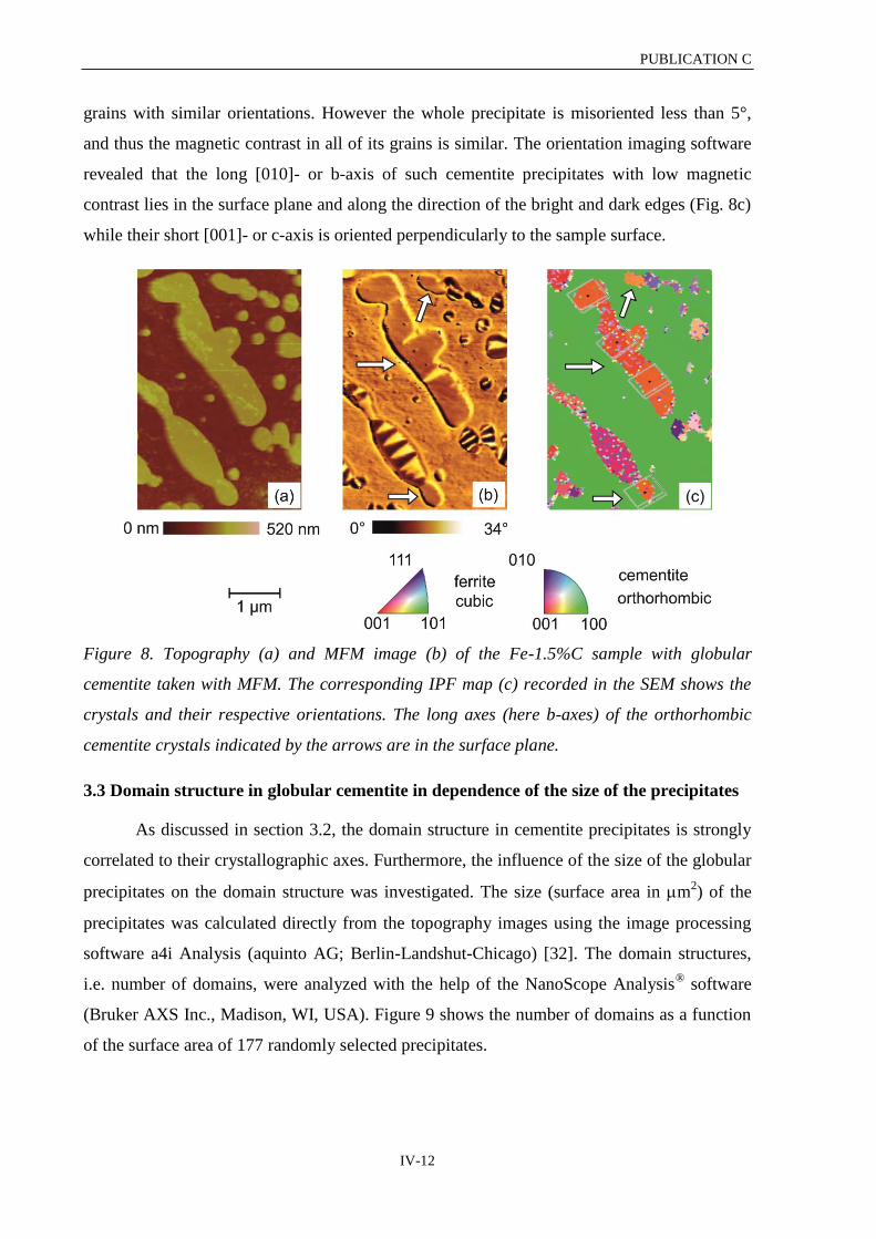
PUBLICATION C
IV-12
grains with similar orientations. However the whole precipitate is misoriented less than 5°,
and thus the magnetic contrast in all of its grains is similar. The orientation imaging software
revealed that the long [010]- or b-axis of such cementite precipitates with low magnetic
contrast lies in the surface plane and along the direction of the bright and dark edges (Fig. 8c)
while their short [001]- or c-axis is oriented perpendicularly to the sample surface.
Figure 8. Topography (a) and MFM image (b) of the Fe-1.5%C sample with globular
cementite taken with MFM. The corresponding IPF map (c) recorded in the SEM shows the
crystals and their respective orientations. The long axes (here b-axes) of the orthorhombic
cementite crystals indicated by the arrows are in the surface plane.
3.3 Domain structure in globular cementite in dependence of the size of the precipitates
As discussed in section 3.2, the domain structure in cementite precipitates is strongly
correlated to their crystallographic axes. Furthermore, the influence of the size of the globular
precipitates on the domain structure was investigated. The size (surface area in m2) of the
precipitates was calculated directly from the topography images using the image processing
software a4i Analysis (aquinto AG; Berlin-Landshut-Chicago) [32]. The domain structures,
i.e. number of domains, were analyzed with the help of the NanoScope Analysis® software
(Bruker AXS Inc., Madison, WI, USA). Figure 9 shows the number of domains as a function
of the surface area of 177 randomly selected precipitates.

PUBLICATION C
IV-13
Figure 9. Plot of the number of domains as a function of the surface area of the cementite
precipitates.
A clear trend can be realized: the larger the area, the higher is the number of domains.
Very small precipitates (up to 5 m2) usually contain not more than 6 domains. Very large
precipitates (> 20 m2), however, may contain more than 10 domains. Some large precipitates
are not single crystals, but have a polycrystalline structure with different grain orientations.
The software a4i analysis calculates the surface area of the whole precipitate without
considering the individual grains separately. As the domain structure of such large precipitates
often extends continuously from one grain to its neighbors, it is reasonable to treat a
precipitate as one unit.
In the samples studied in this work, single-domains were observed in some spherical
cementite precipitates. The single-domain state is energetically favored as long as the stray
field energy is smaller than the wall energy needed for multi-domain formation. Kronmüller
and Fähnle [33] estimated the critical size of a sphere of magnetic material for forming a
single-domain state by
( √ ) ⁄
, (1)
0 [H/m] is the permeability of vacuum, Ms [A/m] is the saturation magnetization, A [J/m] is
the exchange constant, and K1 [J.m-3
] is the single crystal anisotropy. The material parameters
of cementite from the literature, Ms = 9.8 x 10⁵ A/m [34], K1 = 1.18 x 10
5 J.m
-3 [31] and
A = 8.7 x 10⁻¹²
J/m [35], yield the critical diameter for single-domain state forming

PUBLICATION C
IV-14
60 nm. The size distribution and shape of the cementite precipitates depends mostly
on the composition and the thermal treatment of the sample. As shown in the inset (zoom-in
plot, black arrow) in Fig. 9, the smallest detected and analyzed precipitates have an area of
0.1 m2. They are composed of one or two domains. Assuming a spherical shape, their
diameters are about 356.8 nm. These results confirm that, in agreement with theoretical
predictions, even smaller precipitates must be considered in order to reach the critical
diameter for single-domain state in cementite.
3.4 Determination of the easy axis in globular cementite
In order to determine the easy axis of cementite, forty cementite precipitates with
similar size (~ 3 m) and globular shape essentially containing parallel domains were
analyzed with respect to their crystalline orientation. The averaged width of the striped
domains was measured with the help of the NanoScope Analysis®
software (Bruker AXS Inc.,
Madison, WI, USA). Fig. 10a shows in detail the domain structure of a cementite precipitate
oriented close to the (010) plane. An MFM line scan across the domain structure (line
indicated in Fig. 10a) is shown in Fig. 10b. The line scans clearly show the positive and
negative phase shifts in the bright and dark imaged domains, respectively. The average width
of the domains can be measured by evaluating sets of such line scans in selected areas.
Figure 10. Enlarged section of Fig. 2e showing the domain structure of a cementite
precipitate in the Fe-1.5%C sample; (b) line scan across the domain structure, line indicated
in (a). The measured domain thickness in the indicated line scan is 500 nm.
Figure 11a shows a plot of the domain width versus the angle ( between the [010]
direction and the normal to the sample surface. In agreement with the results obtained by Keh
and Johnson [16] using transmission electron microscopy studies on cementite thin foils of
approximately 200 nm thickness, the domain width measured with the MFM shows a clear
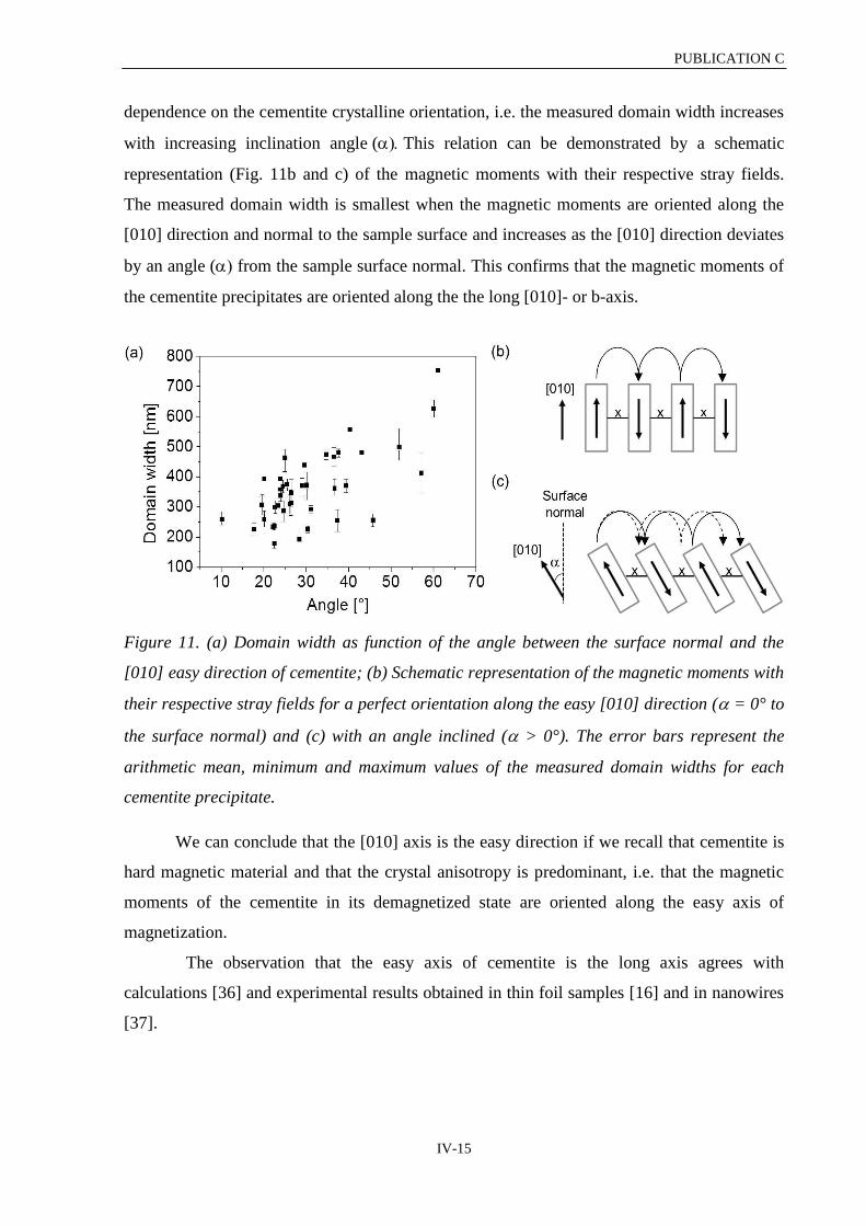
PUBLICATION C
IV-15
dependence on the cementite crystalline orientation, i.e. the measured domain width increases
with increasing inclination angle (This relation can be demonstrated by a schematic
representation (Fig. 11b and c) of the magnetic moments with their respective stray fields.
The measured domain width is smallest when the magnetic moments are oriented along the
[010] direction and normal to the sample surface and increases as the [010] direction deviates
by an angle ( from the sample surface normal. This confirms that the magnetic moments of
the cementite precipitates are oriented along the the long [010]- or b-axis.
Figure 11. (a) Domain width as function of the angle between the surface normal and the
[010] easy direction of cementite; (b) Schematic representation of the magnetic moments with
their respective stray fields for a perfect orientation along the easy [010] direction ( = 0° to
the surface normal) and (c) with an angle inclined ( > 0°). The error bars represent the
arithmetic mean, minimum and maximum values of the measured domain widths for each
cementite precipitate.
We can conclude that the [010] axis is the easy direction if we recall that cementite is
hard magnetic material and that the crystal anisotropy is predominant, i.e. that the magnetic
moments of the cementite in its demagnetized state are oriented along the easy axis of
magnetization.
The observation that the easy axis of cementite is the long axis agrees with
calculations [36] and experimental results obtained in thin foil samples [16] and in nanowires
[37].

PUBLICATION C
IV-16
3.5 MFM images of lamellar pearlite
Figures 12a and b show the topography of the Fe-0.8%C sample containing lamellar
pearlite and the corresponding magnetic microstructure in the demagnetized state,
respectively. For lamellar cementite the determination of the crystalline orientations using
electron diffraction techniques is very difficult because of its low structure factors [38,39].
Figures 13a and b show the phase distribution and the IPF map in one region of the Fe-0.8%C
sample. The identification of the phases, ferrite and cementite, is possible as shown in the
phase distribution map in Fig. 13a. However, the quality of the EBSD patterns (even by spot
EBSD analysis) was insufficient to obtain accurate orientation of the lamellae cementite
crystals (Fig. 13b).
The magnetic domain structures of the lamellar precipitates have similar features to
those observed in the globular precipitates. Some lamellar cementite precipitates (Fig. 12b,
arrow #1) exhibit parallel stripes with strong opposite magnetic contrasts which allows the
conclusion that the magnetic moments of these precipitates are positioned alternately down-
and upwards relative to the surface, and are therefore oriented in or close to the (010) plane.
Other lamellar precipitates (Fig. 12b) show either a relatively strong dark and/or bright (arrow
#2) or a very weak homogeneous magnetic contrast (arrow #3). For the relatively strong dark
and/or bright magnetic contrast the domains are wide and their magnetic moments are
inclined by an angle () with respect to the surface (see Fig. 11c). For the very weak and
homogeneous magnetic contrast the magnetic moments are in-plane oriented. The lamellar
cementite precipitates which show parallel stripes with strong opposite magnetic contrast, and
therefore, oriented in or close to the (010) plane, exhibit higher topographic profiles (Fig. 12a)
compared to the lamellae with other crystalline orientations. This observation can be
explained by the fact that the grinding rate (material removal) during the polishing process of
the surface depends on the material properties which vary not only with the kind of material,
but also with its crystalline orientation. The investigations, therefore, reveal a distinct
correlation of the magnetic domain structure as well as of the surface topography to the
crystalline orientation.

PUBLICATION C
IV-17
Figure 12. Topography (a) and MFM image (b) of the Fe-0.8%C sample with lamellar
cementite taken by MFM.
Figure 13. EBSD maps of the Fe-0.8%C sample with lamellar cementite: (a) phase
distribution map displaying ferrite (gray) and cementite (green) phases and (b) inverse pole
figure (IPF) map, displaying the crystal orientations.
For cementite lamellae with a very large aspect ratio, e.g. of 8 m length and 300 nm
width (Fig. 12b, arrow #4), the magnetic moments still are perpendicularly oriented with
respect to the lamella axis. This observation confirms the high crystal anisotropy of cementite
and that the magnetic domain formation is more dominated by the crystal anisotropy than by
the shape anisotropy. Hence, if the magnetic easy axis is known, the analysis of the MFM
images of the cementite lamellae only allows the estimation of their crystalline orientations.

PUBLICATION C
IV-18
4. SUMMARY
Unalloyed pearlitic steel samples containing globular and lamellar cementite in a
ferrite matrix, respectively, were studied by means of MFM and EBSD techniques. MFM
reveals the topographic and magnetic microstructure, EBSD the local crystalline orientations.
Globular and the lamellar cementite precipitates in steels were chosen as examples to
demonstrate the ability of the combination of MFM and EBSD results to determine the
magnetic easy axes of micro- and nanoscopic precipitates in a bulk material.
In MFM measurements, the choice of an appropriate magnetic probe is crucial for
each particular experiment. For the unalloyed pearlitic steels studied in this work the
commercial MESP probe showed the best contrast and spatial resolution combination. The
MESP probe did not influence the magnetic microstructure of the sample and vice-versa, and
the observed contrast clearly revealed the magnetic microstructure in both phases, ferrite and
cementite.
The combination of MFM and EBSD techniques enables the observation of associated
local topographic, magnetic, and crystallographic microstructures. Bulk samples and
compounds consisting of a matrix with embedded second phase particles can be studied. The
MFM images (spatial resolution down to 50 nm) showed different orientations of the
magnetic moments in the globular and in the lamellar cementite phase. The cementite domain
structure in or around the (010) plane, i.e., the long easy [010]- or b-axis is oriented
perpendicularly to the sample surface was found to consist of parallel stripes of strong
opposite magnetic contrast. The magnetic moments of those precipitates are positioned
alternately down- and upwards in relation to the surface and are separated by 180° domain
walls. For the single crystal precipitates having a large misorientation with respect to the
(010) plane, i.e. oriented close to the (100) plane, a weak dark or bright contrast was
observed, which gives the conclusion that the magnetic moments of those precipitates are
oriented with a small angle ( with respect to the sample surface. The cementite precipitates
oriented in or very close to the (001) plane showed a homogeneous contrast, i.e. very weak
magnetic contrast, leading to the conclusion that their magnetic moments are oriented in-
plane. By means of EBSD the long [010]- or b-axis of the precipitates was determined and
correlated to the magnetic signal. Dark and bright imaged edges of the precipitates confirmed
the in-plane and along the long [010]- or b-axis orientation of the magnetic moments.
Additional MFM and EBSD analysis showed that the width of the domains in the surface is
dependent on the cementite crystalline orientation relative to the surface. The width increases

PUBLICATION C
IV-19
with the angle between the easy [010] axis and the surface normal which confirms the
observations that the magnetic moments are oriented along the long [010]- or b-axis.
In the case for the lamellar cementite precipitates, the EBSD measurements were not
sufficiently accurate to determine the lamellae crystalline orientations. With the previous
knowledge of the behavior of the magnetic domain structure with respect to the crystalline
orientation of the globular precipitates, the crystalline orientation of the cementite lamellae
can be estimated by simply observing the magnetic microstructure and the topographic
profiles.
Finally, we may conclude that the combination of MFM and EBSD techniques allows
determination of the magnetic easy axes of micro- and nanoscopic ferromagnetic precipitates
in a bulk material requiring only relatively simple sample preparation.
REFERENCES
[1] M.T. Johnson, P.J.H. Bloemen, F.J.A. den Broeder, J.J. de Vries, Reports on Progress in
Physics 59 (1996) 1409.
[2] N.P. Goss, Electrical sheet and method and apparatus for its manufacture and test, US
Patent 1.965.559.
[3] N.P. Goss, Transactions of the American Society of Metals 23 (1935) 511.
[4] T. Hayashi, S. Hirono, M. Tomita, S. Umemura, Nature 382 (1996) 772.
[5] K.J. Kirk, Contemporary Physics 41 (2000) 61.
[6] R.C. Jacklevic, J.S. Lambe, A.H. Silver, J.E. Mercerau, Physical Review Letters 12 (1964)
159.
[7] R. Bergholz, U. Gradmann, Journal of Magnetism and Magnetic Materials 45 (1984) 389.
[8] P.J. Flanders, Journal of Applied Physics 63 (1988) 3940.
[9] S. Foner, Journal of Applied Physics 79 (1996) 4740.
[10] J.H.E. Giffiths, Nature 158 (1946) 670.
[11] H. Ebert, Reports on Progress in Physics 59 (1996) 1665.
[12] Z.Q. Ziu, S.D. Bader, Review of Scientific Instruments 71 (2000) 1243.
[13] J.W. Lau, J.M. Shaw, Journal of Physics D: Applied Physics 44 (2011) 303001.
[14] H. Matsuyama, K. Koike, Journal of Electron Microscopy (Japan) 43 (1994) 157.
[15] H. Boersch, H. Raith, Naturwissenschaften 46 (1959) 574.
[16] A.S. Keh, C.A. Johnson, Journal of Applied Physics 34 (1963) 2670.
[17] Y. Martin, H.K. Wickramasinghe, Applied Physics Letters 50 (1987) 1455.
PUBLICATION C
IV-20
[18] J.J. Saenz, N. Garcia, P. Grütter, E. Meyer, H. Heinzelmann, R. Wiesendanger, L.
Rosenthaler, H.R. Hidber, H.J. Güntherodt, Journal of Applied Physics 62 (1987) 4293.
[19] U. Hartmann, Annual Review of Materials Science 29 (1999) 53.
[20] D. Dingley, Journal of Microscopy 213 (2004) 214.
[21] Q. Zhong, D. Inniss, K. Kjoller, V.B. Elings, Surface Science 290 (1993) L688.
[22] X. Zhu, P. Grütter, V. Metlushko, B. Ilic, Journal of Applied Physics 91 (2002) 7340.
[23] A. Alekseev, A. Popkov, A. Shubin, F. Pudonin, N. Djuzhev, Ultramicroscopy 136
(2014) 91.
[24] L. Yue, Z. Li, R. Kirby, D. Sellmyer, Ultramicroscopy 109 (2009) 1040.
[25] (2012). [Online]. Available: http://www.brukerafmprobes.com/.
[26] S. Wust, Untersuchung der magnetischen Domänen in Stahlproben mittels
Magnetkraftmikroskopie unter Anlegen eines externen Magnetfeldes, Diploma thesis,
Saarland University, IZFP report No.110126-TW, Saarbrücken (2011).
[27] Diamond software - Crystal and Molecular Structure Visualization, Crystal Impact,
Bonn, Germany, http://www.crystalimpact.com/diamond.
[28] C. Jiang, S.G. Srinivasan, A. Caro, S.A. Maloy, Journal of Applied Physics 103 (2008)
043502.
[29] L. Batista, U. Rabe, S. Hirsekorn, NDT & E International 57 (2013) 58.
[30] L. Batista, U. Rabe, I. Altpeter, S. Hirsekorn, G. Dobmann, Journal of Magnetism and
Magnetic Materials 254 (2014) 248.
[31] P. Blum, R. Pauthenet, Comptes Rendus 237 (1953) 1501.
[32] a4i Analysis, Version 5.10a; aquinto AG; Berlin-Landshut-Chicago
http://www.aquinto.com.
[33] H. Kronmüller, M. Fähnle, Micromagnetism and the Microstructure of Ferromagnetic
Solids, Cambridge University Press, Cambridge (2003).
[34] F. Stäblein, K. Schroeter, Zeitschrift für anorganische und allgemeine Chemie 174
(1928) 193.
[35] W. Lottermoser, A.K. Schaper, W. Treutmann, G. Redhammer, G. Tippelt, A.
Lichtenberger, S.-U. Weber, G. Amthauer, Journal of Physical Chemistry B 110 (2006) 9768.
[36] A.K. Arzhnikov, L.V. Dobysheva, C. Demangeat, Journal of Physics: Condensed Matter
19 (2007) 9.
[37] U. Weissker, M. Löffler, F. Wolny, M.U. Lutz, N. Scheerbaum, R. Klingeler, T.
Gemming, T. Mühl, A. Leonhardt, B. Büchner, Journal of Applied Physics 106 (2009)
054909.

PUBLICATION C
IV-21
[38] S. Zaefferer, S.I. Wright, D. Raabe, Metallurgical and Materials Transactions A 39A
(2008) 374.
[39] T. Takahashi, D. Ponge, D. Raabe, Steel Research International 78 (2007) 38.

IV-22
PUBLICATION D
V-1
V. CHARACTERIZATION OF THE MAGNETIC MICRO- AND
NANOSTRUCTURE IN UNALLOYED STEELS BY MAGNETIC FORCE
MICROSCOPY (PUBLICATION D)
L. Batista, U. Rabe, and S. Hirsekorn
AIP Conference Proceedings (2013) Vol. 1511; 1180-1187.
ABSTRACT. The formation of a cementite phase influences significantly the macroscopic
mechanical and magnetic properties of steels. Based on a correlation between mechanical and
magnetic properties, mechanical properties as well as the morphology and content of the
cementite phase can be inspected by electromagnetic non-destructive testing methods. The
influence of the carbon content on bulk magnetic properties of unalloyed steels is studied on a
macroscopic scale by hysteresis loop and Barkhausen noise measurements. The micro- and
nanostructure is investigated by atomic force microscopy and magnetic force microscopy.
Surface topography images and magnetic images of globular cementite precipitates embedded
in a ferrite matrix are presented. The size, shape, and orientation of the precipitates influence
the domain configuration. Applied external magnetic fields cause magnetization processes
mainly in the ferrite matrix: Bloch walls move and are pinned by the cementite precipitates.
The correlation between the microscopic observations and macroscopic magnetic properties
of the material is discussed.
Keywords: Atomic Force Microscopy (AFM), Magnetic Force Microscopy (MFM), Electron
Backscattering Diffraction (EBSD), Steel, Microstructure, Nanostructure, Magnetic domains,
Non-destructive testing

PUBLICATION D
V-2
1. INTRODUCTION
Steels constitute the most widely used category of metallic materials because they
provide a wide range of mechanical properties and can be manufactured relatively
inexpensively in large quantities to very precise specifications [1]. Among all the phases or
constituents that can be obtained by choosing the chemical composition, thermomechanical
treatment, etc., two are frequently encountered in most of technical steels: ferrite and
cementite. The volume fraction and morphology of the cementite phase controls directly the
mechanical and magnetic properties of steels.
The bulk macroscopic magnetic properties of steels containing cementite embedded in
a ferrite matrix have already been studied by many authors [2-5]. Even though several studies
have been done using the magnetic Barkhausen noise (MBN) technique, a clear understanding
on the individual influence of the cementite phase on the generation of the MBN has still not
been well established. For example, the MBN activity profile in a microstructure containing
cementite in a ferrite matrix has been observed as a single [4] as well as a double peak
behavior [5].
All these macroscopic observations rely on a phenomenological description of the
interactions of the magnetic domains with the microstructure. The microscopic magnetic
domain structures can be imaged by different techniques. For example, domains in high-
permeability materials were imaged by Kerr microscopy [6] and the domain configuration of
a cementite thin foil was revealed by Lorentz electron microscopy [7]. Magnetic Force
Microscopy (MFM) has been widely employed to map magnetic structures of surfaces [8-13].
In addition to its high local resolution in the range of 10 nm MFM has the ability to measure
the topography and the magnetic microstructure simultaneously allowing the study of
interaction between defects and magnetic properties.
In this paper, samples of a high purity polycrystalline iron and of two unalloyed steels
(Fe-0.8%C and Fe-1.5%C) containing globular cementite embedded in a ferrite matrix were
investigated. In the first part of this work, the macroscopic magnetic quantities, i.e. saturation
magnetization, coercive field and maximum Barkhausen noise amplitude were measured and
interpreted with respect to the microstructural state. In the second part, the magnetic
microstructures were observed using a Magnetic Force Microscope. The MFM was coupled
with an external coil providing a controlled in-plane magnetic field which allowed the
observation of the dynamic behavior of the magnetic domains. Ferromagnetic domains were
studied in the high purity polycrystalline iron sample and in the cementite and ferrite phases
of the unalloyed steels. By means of Electron Backscatter Diffraction (EBSD) the crystalline

PUBLICATION D
V-3
orientation of the cementite particles and the ferrite phase, respectively, were determined. The
correlation between the macroscopic magnetic properties and the magnetic and
crystallographic microstructure was examined.
2. MATERIALS AND METHODS
2.1 Unalloyed steels: Fe–C systems (Fe–Fe3C)
Samples of high purity iron (99.99%) and of two unalloyed steels, Fe-0.8%C and Fe-
1.5%C, containing globular cementite (Fe3C) in a ferrite matrix were provided as-cast and
machined in a cylindrical shape of 8 mm diameter and 50 mm length. Subsequently the
samples were vacuum annealed at 600°C for 4h in order to remove all processing-induced
residual stresses. The resulting microstructure has an average grain size of approximately
80 m for all samples. The size of the cementite precipitates ranges from a few hundred
nanometers to about 10 m in diameter.
For AFM and MFM measurements small specimens (3 x 3 x 1 mm3) were cut from the
annealed cylindrical samples by spark erosion and mechanically polished by standard
procedures. Directly before the measurements, the samples were slightly etched using Nital
(95% Ethanol + 5% Nitric acid) in order to obtain reproducible surface conditions.
2.2 Bulk magnetic properties: hysteresis loop and Barkhausen noise signals
The hysteresis loop and Barkhausen noise measurements were performed inside an
electromagnet with a bipolar power supply controlled by a function generator. The magnetic
field strength was measured by a Hall probe. The cylindrical samples were magnetized along
their axial direction reaching a maximum magnetic field strength of 110 A/cm at an excitation
frequency of 0.5 Hz. The change in magnetic flux density and the inductive Barkhausen noise
of the cylindrical samples were measured by a surrounding pick-up coil. The voltage induced
by the noise signals was recorded as a function of the tangential field strength.
The magnetic hysteresis curves and the Barkhausen noise curves of the three samples
are shown in figures 1a-c as dotted and continuous curves, respectively. The coercivity Hc
increases with carbon content, while the relative permeability at the coercive field Hc and the
saturation magnetization BS at 100 A/cm decrease with increasing carbon content. This
indicates that the magnetic hardness increases as the carbon content increases. The measured
parameters are listed in Table 1. The Barkhausen noise curves are remarkably different in
their shape (single and double peaks) and in their maximal amplitude values. High peaks
(fig. 1a) close to the coercive field Hc are observed for the high purity iron sample showing

PUBLICATION D
V-4
the easy irreversible domain wall movement (mostly 180° BWs) through the microstructure.
The addition of 0.8 and 1.5 wt. % carbon, respectively, results in a microstructure with
globular cementite precipitates embedded in a ferrite matrix with less than 0.008 wt. % of
carbon in solid solution. A broadening of the Barkhausen noise peak and a decreasing peak
height can be observed as shown in the continuous curves of figures 1b and c, respectively.
This can be attributed to the interstitial carbon atoms in the ferrite matrix and the intra- and
intergranular cementite precipitates. Furthermore, the Barkhausen noise signals of the samples
with cementite precipitates clearly show double peaks. The lower field peak corresponds to
the ferrite and the higher field peak to the cementite phase. The amplitude of the peaks seems
to be proportional to the amount of each phase. Increasing the amount of carbon the ferrite
peak decreases and the cementite peak increases (figs. 1b and c). This can be explained due to
the fact that the magnetization and respective Barkhausen jumps in the cementite phase occur
at higher fields.
Figure 1. Hysteresis loop (dotted line) and Barkhausen noise (continuous line) curves for (a)
pure Fe (99,99%) and two unalloyed steels containing different content of globular cementite
(b) Fe-0.8%C and (c) Fe-1.5%C. The measurements were performed at 1.8 V and 0.5 Hz.
Table 1. Parameters deduced from the macroscopic measurements shown in figure 1.
Carbon
content
[wt%]
Coercive
field HC
[A/cm]
Relative
permeability
at Hc
Saturation
magnetization BS
[T]
Maximum
Barkhausen noise
amplitude Mmax [mV]
0 (Pure Fe) 4.2 0.17 1.96 14.2
0.8 6.8 0.13 1.75 11.5
1.5 8.2 0.11 1.55 9.5

PUBLICATION D
V-5
2.3 Local magnetic properties – magnetic force microscope (MFM) with a superposed
external magnetic field
Atomic force microscopy (AFM) and MFM have been used to image the topography
and the magnetic microstructure of the samples, respectively. The measurements were
performed in tapping-lift mode using a commercial AFM/MFM instrument (Nanoscope III®
multimode, Digital Instruments, Santa Barbara, CA, USA). The sensor tips were CoCr-coated
with a coercivity of ~ 320 A/cm MESP, Bruker AXS Inc., Madison, WI, USA). A lift-height
of 60 to 80 nm was chosen for all measurements reported here. In order to investigate the
evolution of the magnetic microstructure and the resulting domain configuration, an external
electromagnet was combined with the MFM as shown in figure 2. The pole shoes of the
electromagnet were adjusted such that the sample inside the AFM was magnetized parallel to
its surface. All magnetic images presented in this work are so-called phase images, i.e. the
local phase shift was recorded as a function of position.
2.4 MFM images of the high purity bulk iron
Figure 3a shows the topography image obtained with the MFM of the high purity iron
bulk sample revealing the grain structure having height differences up to about 100 nm. The
corresponding magnetic microstructure is shown in fig. 3b. Each grain has its own domain
structure depending mostly on the crystalline orientation and residual stress levels. For
example, grain (1) shows large areas with an almost homogeneous grey level, while grain (2)
displays a multitude of small areas with different magnetic contrast. The domain arrangement
at the surface is primarily determined by the principle of flux closure which minimizes the
total inner energy. Additionally, it is strongly dependent on the surface orientation relative to
the easy directions. From the simplest case, i.e. a surface containing two easy axes, to strongly
disoriented surfaces with no easy axis, the domain patterns become progressively more
complicated [14]. The <001> directions are the easy directions for iron and therefore the
(100) surface contains two mutually perpendicular easy directions. This allows us to conclude
that the orientation of the grain (1) is close to the plane (100), and the orientation of the grain
(2) strongly deviates from the plane (100). The domain patterns often face deviations from the
ideal structure because of residual stresses and possibly induced anisotropies.

PUBLICATION D
V-6
Figure 2. (a) Photograph of the experimental set-up for the MFM measurements coupled with
an external coil providing a controlled in-plane magnetic field. (b) Corresponding drawing
showing the coil (1), yoke (2), MFM base (3), and MFM head (4), respectively.
Figure 3. Topography (a) and MFM image (b) of the high purity bulk iron sample taken with
MFM.
Figures 4 a-d demonstrate the evolution of the magnetic microstructure for the high
purity iron sample in an external in-plane magnetic field. The imaged area is located in a grain
oriented close to (100) surface. The image displays a few domains clearly separated by Bloch
walls which can be detected as bright or dark lines in the MFM image (white arrows in fig. 4).
At the remanence state, a domain wall will be in a position which minimizes the energy of the
system formed by the wall itself and the adjoining domains and domain walls. Most domain
walls are bulged possibly indicating the existence of defects and residual microstress, which is
caused by crystal imperfections as e.g. dislocations [15].
When a magnetic field is applied, a change of position of the domains can be
observed. For example a domain wall (dark line) indicated by a white arrow in figs. 4 moves
downwards as the field strength increases. Another domain wall (bright line) also indicated by

PUBLICATION D
V-7
a white arrow moves upwards. Accordingly, the supplementary domains between the black
and white walls disappear.
Figure 4. MFM images of the high purity iron sample (a) without external field and with an
applied external field of (b) 100 A/cm, (c) 160 A/cm, and (d) 190 A/cm, respectively. The
direction of the in-plane field is indicated by black arrows above the images.
2.5 MFM and EBSD images of samples containing globular cementite embedded in a
ferrite matrix
The unalloyed steels Fe-0.8%C and Fe-1.5%C investigated in this work consist of a
relatively hard magnetic cementite phase embedded in a soft ferromagnetic ferrite matrix. The
cementite content is higher in the Fe-1.5%C sample than in the Fe-0.8%C-sample, but the
basic behavior of the magnetic microstructure can be discussed by considering only the Fe-
1.5%C as an example.
Figure 5a shows the topography obtained with the MFM of the Fe-1.5%C sample
revealing the microstructure and surface roughness. The cementite precipitates appear higher
than the ferrite matrix with an offset of about 400 nm maximum. Two grains with different

PUBLICATION D
V-8
average height numbered (1) and (2) are visible in the ferrite matrix. The corresponding
magnetic microstructure in the demagnetized state as well as the Electron Backscatter
Diffraction (EBSD) map taken in the same area with a Scanning Electron Microscope, i.e. the
Inverse Pole Figure (IPF), are shown in figs. 5b and 5c, respectively. The color code of the
inverse pole figure represents the crystallographic orientation in the ferrite matrix (nearly pure
b.c.c. iron, lattice constant a = 2.87Å), and in the cementite particles (orthorhombic
symmetry, length of the three perpendicular axes a = 5.09Å, b = 6.74Å, c = 4.52Å). Using an
orientation imaging software, the angles of inclination of the two ferrite grains (1) and (2)
relative to the (100) plane were obtained as 9° and 15°, respectively. The ferrite matrix
(fig. 5b) shows a complex domain configuration displayed by a multitude of small areas with
different magnetic contrast. Spike domains [16] are formed on the cementite/ferrite interface,
which can be attributed to stresses due to differences in thermal expansion coefficient of the
two phases and reduction of the cementite magnetostatic energy. Orange arrows in fig. 5b
point to a domain in the ferrite matrix, which is limited in size by a grain boundary on the
right and by a cementite precipitate on the left side. It is well known that grain boundaries as
well as precipitates contribute to increase the magnetic hardness of ferromagnetic materials by
restricting the movement of domain walls.
Figure 5. Topography (a) and MFM image (b) of the Fe-1.5%C sample taken with MFM. The
corresponding IPF map recorded in the SEM shows the crystals and their respective
orientations. Two ferrite grains with different crystal orientation are marked as (1) and (2) in
the topography image.

PUBLICATION D
V-9
The cementite precipitates show a much stronger magnetic image contrast than the
ferrite matrix because cementite is magnetically harder than ferrite and thus causes stronger
stray fields. The domains observed in the cementite precipitates range from 50 to 1000 nm in
width depending on their crystalline orientation. The cementite precipitates in or around the
(010) orientation presents always a stripe structure. Since the MFM tip senses the component
of the stray field emerging perpendicularly from the surface, we may conclude that the
magnetic moments of these precipitates are more or less parallel to the tip axis, i.e.
perpendicular to the sample surface plane and oriented along the long axis (here [010]- or
b-axis).
An example for a Barkhausen jump is shown in figures 6. Figure 6a shows the
topography obtained with the MFM of the Fe-1.5%C sample, and the evolution of the
magnetic microstructure under a superposed applied magnetic field is shown in figs. 6b and c.
Figure 6b is recorded at the remanence state of the sample while fig. 6c displays the results
with an applied magnetic field of 190 A/cm. Bright and dark lines are visible within the ferrite
matrix, which can be identified as domain walls. Initially, if the magnetic field is smaller than
the coercive field (H < Hc), the domain wall is attached to pinning points (fig. 6b). When
H > Hc, the domain wall unpins, propagates and pins to the next precipitate (fig. 6c, white
arrow). These microscopic observations make clear that an increase of the amount of carbon
and consequently an increase of the amount of pinning sites can cause a decrease of the
macroscopic initial permeability and an increase of coercivity.
Figure 6. Topography (a) of the sample Fe-1.5%C containing globular cementite precipitates
in a ferrite matrix, MFM images taken (b) without external magnetic field and with an applied
field of (c) 190 A/cm. The direction of the in-plane field is indicated by a black arrow. The
white arrows indicate a domain wall movement.

PUBLICATION D
V-10
3. SUMMARY
The combination of AFM, MFM, and EBSD techniques with macroscopic magnetic
measurements opens a new field for material development and design enabling the direct
observation of magnetic micro- and nanostructures including the corresponding single crystal
grain orientations. Samples of highly pure iron and the unalloyed steels Fe-0.8%C and Fe-
1.5%C were characterized macroscopically by measuring hysteresis loops and Barkhausen
noise signals. The magnetic hardness increases with increasing amount of carbon in form of
globular cementite precipitates in the ferrite matrix. Besides, the Barkhausen noise amplitude
decreases and becomes a double peak. The weaker field peak corresponds to the ferrite and
the stronger field peak to the cementite phase.
MFM was shown to be a powerful tool for nondestructive magnetic microstructure
imaging and characterization in the micro- and nanoscale of steels. In this work, MFM images
with a local resolution of 50 nm have been achieved. The crystalline orientation of the ferrite
and cementite phases were determined by EBSD and correlated to the domain structure.
Ferromagnetic domain structures in highly pure iron and in cementite precipitates as well as
their interaction were studied. Domain walls in the ferrite phase tend to intersect the cementite
precipitates in order to minimize the magnetostatic and wall energy. By applying an external
in-plane magnetic field the dynamic behavior of the magnetic domains and the interaction
between domain walls and the cementite precipitates was observed and characterized.
REFERENCES
[1] ASM International Handbook (1990). ASM Handbook, Volume 1 - Properties and
Selection: Irons, Steels, and High Performance Alloys, Materials Park, OH, ASM
International, page 233.
[2] I. Altpeter, Journal of Nondestructive Evaluation 15 (1996) 45.
[3] I. Altpeter, G. Dobmann, M. Kröning, M. Rabung, S. Szielasko, NDT&E International 42
(2009) 283.
[4] M. Blaow, J.T. Evans, B.A. Shaw, Acta Materialia 53 (2005) 279.
[5] V. Moorthy, S. Vadyanathan, T. Jayakumar, B. Raj, Journal of Magnetism and Magnetic
Materials 171 (1997) 179.
[6] R. Schäfer, Journal of Magnetism and Magnetic Materials 215-216 (2000) 652.
[7] A.S. Keh, C.A. Johnson, Journal of Applied Physics 34 (1963) 2670.
[8] P. Grütter, T. Jung, H. Heinzelmann, A. Wadas, E. Meyer, H.R. Hidberand, H.J.
Güntherodt, Journal of Applied Physics 67 (1990) 1437.

PUBLICATION D
V-11
[9] Y. Martin, H.K. Wickramasinghe, Applied Physics Letters 50 (1987) 1455.
[10] J.J. Saenz, N. Garcia, P. Griitter, E. Meyer, H. Heinzelmann, R. Wiesendanger, L.
Rosenthaler, H.R. Hidber, H.J. Güntherodt, Journal of Applied Physics 62 (1987) 4293.
[11] S. Huo, J.E.L. Bishop, J.W. Tucker, M.A. Al-Khafaji, W.M. Rainforth, H.A. Davies,
M.R.J. Gibbs, Journal of Magnetism and Magnetic Materials 190 (1998) 17.
[12] L. Batista, U. Rabe, S. Hirsekorn, "Micro- and Nanostructure Imaging and
Characterization of Advanced Steels", 38th Annual Review of Progress in Quantitative
Nondestructive Evaluation (QNDE), July 17-22, 2011, Burlington, Vermont, USA.
[13] L. Batista, U. Rabe, S. Hirsekorn, Magnetic micro- and nanostructures of unalloyed
steels: domain wall interactions with cementite precipitates observed by MFM, in review.
[14] A. Hubert, R. Schäfer, Magnetic Domains - The Analysis of Magnetic Microstructures,
Springer, Berlin (1998).
[15] B.D. Cullity, Introduction to magnetic materials, Addison Wesley, London (1972).
[16] H.J. Williams, Physical Review 71 (1947) 646.

V-12

PUBLICATION E
VI-1
VI. MICRO- AND NANOSTRUCTURE CHARACTERIZATION AND IMAGING
OF TWIP AND UNALLOYED STEELS (PUBLICATION E)
L. Batista, U. Rabe, and S. Hirsekorn
AIP Conference Proceedings (2012) Vol. 1430; 1381-1388.
ABSTRACT. New design concepts for constructing light-weight and crash resistant
transportation systems require the development of high strength and supra-ductile steels with
enhanced energy absorption and reduced specific weight. TWIP steels combine these
properties, a consequence of intensive mechanical twinning. To understand the mechanisms,
related microstructures and local material properties are probed by AFAM, nanoindentation,
and EBSD. The morphology of a cementite phase controls the macroscopic mechanical and
magnetic properties of steels. Cementite embedded in a ferrite matrix is characterized by
AFAM and MFM.
Keywords: Atomic Force Acoustic Microscopy, Imaging, Magnetic Force Microscopy,
Microstructure, Nanostructure, Steel

PUBLICATION E
VI-2
1. INTRODUCTION
The current strong demand for vehicle lightening from the automobile sector requires
flat carbon steel sheet manufacturers to develop new advanced grades capable of fulfilling the
contradicting properties such as weight reduction and formability versus high stiffness and
strength. Austenitic twinning induced plasticity (TWIP) steels have low to intermediate
stacking fault energy and hence undergo extensive mechanical twinning during deformation,
which in turn leads to an excellent combination of strength, ductility, and damage tolerance
satisfying the requirements for automotive industries [1]. The main mechanical properties of
these alloys have been investigated by many authors using standard destructive techniques
[2-5]. The optimization of microstructures opens a new field for the design of new alloys.
This requires the understanding of the macroscopic elastic and plastic properties in relation to
the microstructure. In this contribution, the near-field technique atomic force acoustic
microscopy (AFAM) [e.g. 6-11] which combines atomic force microscopy (AFM) [12] with
ultrasound is used to image microstructures and probe material properties on the micro- and
nanoscale. AFAM is a contact resonance spectroscopy technique with a spatial resolution
down to the nm range and, similar to nanoindentation, sensitive to the local indentation
modulus accounting for normal and shear deformation in the tip-sample contact zone.
In the second part of this work, an unalloyed steel Fe-0.8%C is studied by means of
atomic force acoustic microscopy (AFAM) and magnetic force microscopy (MFM).
Cementite (Fe3C) is an important phase in steels because its morphology directly controls
mechanical and magnetic properties. In contrast to its technological significance, the
knowledge about the elastic properties of Fe3C is quite limited. A large scatter on the value
for the Young´s Modulus can be found in the literature [13-18]. The macroscopic magnetic
properties of unalloyed steels have already been studied by many authors [e.g. 19,20].
Microstructure parameters such as lattice defects and grain and phase boundaries impede
temporarily magnetic domain wall movements under magnetic load and thus reveal about
mechanical material properties [21]. Therefore, a MFM coupled with an external coil
providing an in-plane controlled magnetic field is employed to image the dynamic behavior of
magnetic domains and related microstructures.

PUBLICATION E
VI-3
2. MATERIALS AND METHODS
2.1 Twinning-induced plasticity (TWIP) steels
Two different kinds of TWIP based 100% austenitic alloys are investigated. They
were provided after hot-rolling, 50% cold-rolling, and annealing. The chemical composition
(wt%) of the sheets are Fe-22Mn-0.6C-0.2V and Fe-20Mn-3Si-3Al with average grain sizes
of 1 μm and 40 μm, respectively. Both sheets have a monomodal grain size distribution, a
thickness of 1.2 mm, and show macroscopically isotropic material behavior. The elastic
properties were measured by ultrasound in different directions. The isotropic plastic behavior
was shown by tensile tests performed at small samples taken in rolling and in transverse
direction. For AFAM and nanoindentation measurements small specimens were cut by spark
erosion from the recrystallized and annealed steel sheets and mechanically polished by
standard procedures. Directly before the measurements, in order to obtain suitably
reproducible surface conditions, the samples were electropolished which removed a surface
layer of about 1-2 µm. The AFAM and nanoindentation experiments were carried out with a
Dimension 3000® from Digital Instruments (DI) and a Hysitron Triboscope
® in conjunction
with a DI Nanoscope II, respectively.
The microstructure evolution during tensile load of Fe-22Mn-0.6C-0.2V (wt%) TWIP
alloy was monitored. The investigation was performed by an experimental set-up composed
of an AFM (Dimension 3000®) and a tensile machine (UTS, electromechanical). In order to
avoid residual stresses the bone-shaped tensile test samples were also cut by spark erosion.
AFM observations and EBSD analysis require specific sample surface preparation. In order to
observe very small deformation induced relief in the AFM images and to be able to probe
local mechanical properties, the surfaces have to be perfectly plane. Thus, the sample was
polished mechanically by standard procedures followed by electrochemical polishing.
Suitable electrolyte as well as exposure time and voltage have to be identified and selected
very carefully by series of experiments. After preparation, the surface roughness was
evaluated statistically from AFM micrographs 3 μm x 3 μm in size. The best result obtained
was a roughness of RMS < 1 nm. The sample was marked with a microindenter, and the grain
orientations were determined by EBSD. The specimen was deformed with engineering plastic
strains of εp = 3%, 6%, 10%, and 15%. After each deformation step the tensile test was
interrupted and AFM images were taken in contact mode. The tests were carried out in air at
room temperature.

PUBLICATION E
VI-4
2.2 Unalloyed steel (Fe-0.8%C)
The unalloyed steel Fe-0.8%C sample examined in this work was provided as-cast and
annealed in a cylindrical shape of 8 mm diameter with a microstructure of globular cementite
(Fe3C) embedded in a ferrite matrix. From the cylindrical sample, a 1 mm thick disk shape
was cut by spark erosion and prepared as described in the previous section.
2.3 Quantitative AFAM and nanoindentation compared to EBSD maps
In order to probe local elastic properties of the TWIP steels, AFAM as well as
nanoindentation was applied. In AFAM, from measured local contact resonance frequencies
of an AFM cantilever local indentation moduli of the sample surface are determined by
calibration or by calculation via the Hertzian contact theory if the shape and the material
properties of the cantilever and sensor tip are known well enough [e.g. 11].
Figure 1 shows EBSD maps and AFM topography images of nanoindents in the steels
Fe-22Mn-0.6C-0.2V (Fig. 1a) and Fe-20Mn-3Si-3Al (Fig. 1b). To be able to probe the local
mechanical properties in correlation to the grain orientation, the samples were previously
marked by focused ion beam (Fig. 1a) and microindentation (Fig. 1b). In accordance to the
ultrasonic measurements (see materials description above) the EBSD maps show no preferred
grain orientation. The indentation moduli for different grain orientations are given in Table 1.
All results show the same correct trend, i.e. stiffness in or around (111) direction is higher
than in or around (101) direction which is higher than in or around (001) direction. The
differences in AFAM and nanoindentation results might be caused by different tip shapes,
different sizes of involved surface area, and inaccuracies in the AFAM calibration.
Figure 2 shows a series of AFM contact mode topography images of a surface area of
the Fe22Mn0.6C-0.2V specimen for different plastic deformation levels revealing a typical
evolution of the surface relief during a tensile test of TWIP steel. Fig. 2a presents the selected
surface area before loading. It contains height differences up to about 100 nm and clearly
reflects the grain structure (already imaged and confirmed by ArcelorMittal, who provided us
with the samples). The grain boundaries appear higher than the grains itself, i.e. the
preparation of the sample surface generates prominent grain boundaries. Such a relief is
probably due to a preferential attack of grain interiors during electrolytic polishing. For 3%
plastic strain, the AFM image already shows mechanical twinning in the austenite grains
appearing as nearly equidistant straight lines (Fig. 2b). Increasing plastic strain (6, 10, and
15%) causes increasing twinning area fractions. Mechanical twinning creates a step the height
of which can be accurately measured by AFM. Fig. 3 presents the height profiles in the area

PUBLICATION E
VI-5
pointed by a black arrow in Fig. 2 for the different plastic strain levels indicating an increase
in step height with increasing plastic deformation. The EBSD map in Fig. 2f reveals the grain
orientations in the sample surface at 15% deformation (see color code in the legend). The
presence of twins is confirmed by the straight lines having different orientations than the
austenite grain itself. AFM observations of the surface relief have already been reported, e.g.
in 316L austenitic [22–24] and in duplex stainless steel [25]. However, the observation of
surface relief due to mechanical twinning is presented for the first time. The determination of
the involved slip planes during formation of the twins in relation to the surface relief is a topic
of current work.
Figure 1. EBSD (Electron Backscattering Diffraction) images for single grain orientation
determination and AFM topography images showing the nanoindentation marks in the
austenitic TWIP steels: (a) Fe-22Mn-0.6C-0.2V, average grain size 1 μm and (b) Fe-20Mn-
3Si-3Al, average grain size 40 μm.
Table 1. Indentation moduli (M) of the TWIP steels Fe-22Mn-0.6C-0.2V and Fe-20Mn-3Si-
3Al with average grain sizes of 1 μm and 40 μm, respectively.
M (GPa) from quantitative
AFAM M (GPa) from nanoindentation
(111) (101) (001) (111) (101) (001)
FeMnC (V) 179 167 139 218 207 197
FeMnC (Al,Si) 171 142 113 160 134 131

PUBLICATION E
VI-6
Figure 2. Series of AFM micrographs documenting the evolution of surface relief topography
in Fe-22Mn-0.6C-0.2V TWIP steel during a tensile test: (a) before loading; (b, c, d and e)
with plastic strains of 3%, 6%, 9%, and 15%, respectively; (f) EBSD map showing the grain
orientations after 15% plastic stain. The loading direction is indicated in (b).
Figure 3. Series of AFM height profiles measured in Fe-22Mn-0.6C-0.2V TWIP steel with
different plastic strain levels. The height profiles were measured in the same area as pointed
by a black arrow in Fig. 2.
2.4 Magnetic force microscopy (MFM) combined with EBSD (sample Fe-0.8%C
unalloyed steel)
AFM and MFM have been used to image the topography and the magnetic
microstructure of the unalloyed steel Fe-0.8%C containing globular cementite embedded in a
ferrite matrix. The measurements were performed in tapping-lift mode using a Nanoscope III®

PUBLICATION E
VI-7
multimode from DI and MESP CoCr-coated tips with a coercivity of ~ 400 Oe. The CoCr-
coated tips are magnetized along the tip axis by a permanent magnet. A height of 60 to 80 nm
above the sample surface was kept during measurement. The images acquired at the
remanence and with a superposed magnetic field of different strength by means of an external
coil reveal the magnetic microstructure and the evolution of the resulting domain
configuration. In cubic crystals as in the case of the ferrite the domain patterns are determined
by the surface orientation relative to the easy directions. From the simplest case, a surface
with two easy axes, to strongly mis-oriented surfaces with no easy axis, the domain patterns
become progressively more complicated [26]. The domain arrangement is primarily
determined by the principle of flux closure which minimizes the total inner energy.
In ferrite the surface (100) contains two easy directions reducing the complexity for
image interpretations. However, the domain patterns often face deviations from the ideal
structure because of residual stresses and possible induced anisotropies. The domains in the
ferrite matrix, generally in the form of closure domains, often appear to be unrelated to the
domains in the cementite. The domains observed in the cementite particles range from 50 to
1000 nm in width depending on their orientation. The cementite particles in or around the
(010) orientation present always a stripe structure showing perpendicular anisotropy.
Supplementary domains can be seen at the interface between the ferrite and the cementite
phases (white arrows in Fig. 4) which is typical for a pattern containing stresses. This can be
explained by differences in the thermal expansion coefficient of the two phases creating
residual stresses while cooling [20]. The MFM images show increasing size of supplementary
domains with increasing in-plane magnetic field.
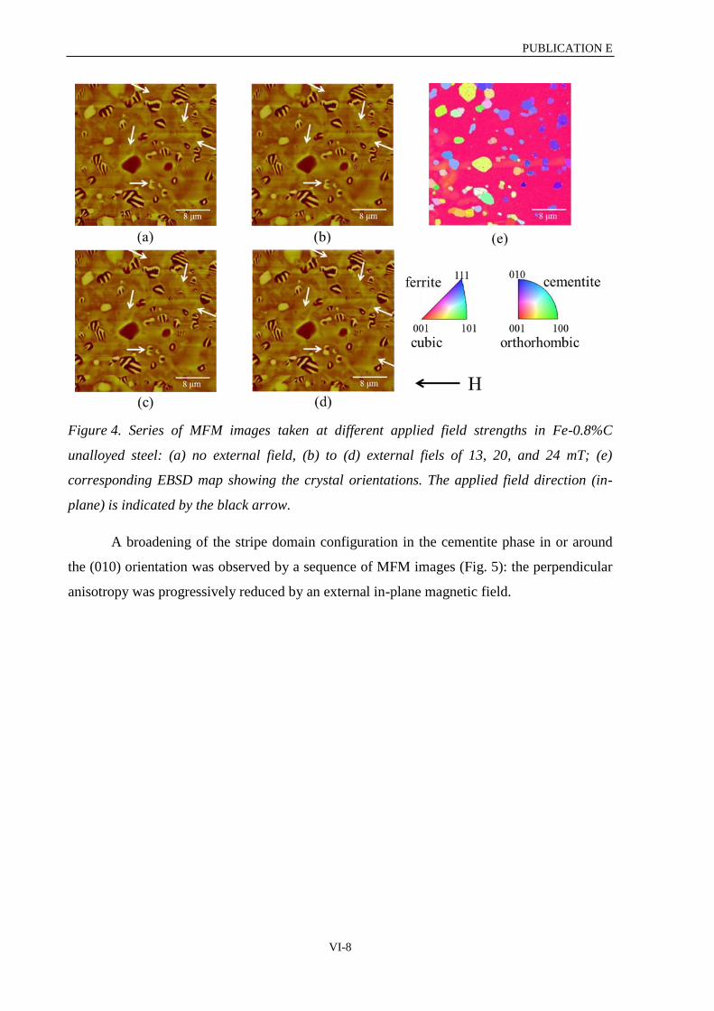
PUBLICATION E
VI-8
Figure 4. Series of MFM images taken at different applied field strengths in Fe-0.8%C
unalloyed steel: (a) no external field, (b) to (d) external fiels of 13, 20, and 24 mT; (e)
corresponding EBSD map showing the crystal orientations. The applied field direction (in-
plane) is indicated by the black arrow.
A broadening of the stripe domain configuration in the cementite phase in or around
the (010) orientation was observed by a sequence of MFM images (Fig. 5): the perpendicular
anisotropy was progressively reduced by an external in-plane magnetic field.

PUBLICATION E
VI-9
Figure 5. Series of images of Fe-0.8%C unalloyed steel showing the evolution of the
cementite magnetic structure with an applied external magnetic field: (a) topography image;
MFM images without (b) and with external field of (c) 13 mT and (d) 24 mT; (e)
corresponding EBSD map showing the crystal orientations. The applied field direction (in-
plane) is indicated by the black arrow.
2.5 In-situ elasticity mapping of cementite precipitates in Fe-0.8%C unalloyed steel
In this work, unalloyed steel Fe-0.8%C containing globular cementite was studied, i.e.
cementite embedded in a ferrite matrix but not isolated cementite, which presents many
difficulties during its preparation. Fig. 6a shows an optical micrograph of the steel. The
topography (Fig. 6b) reveals microstructure and surface roughness. The cementite precipitates
appear higher than the ferrite matrix with an offset of about 20 nm maximum.
AFAM amplitude images yield qualitative surface elasticity maps [e.g. 27]. While the
sample surface is scanned the AFM cantilever is excited to vibrations at a fixed ultrasonic
frequency close to a contact resonance. The cantilever vibration amplitude and thus the
AFAM image contrast depends on the difference between the excitation frequency and the
local contact resonance. Fig. 6c is recorded with a 622 kHz excitation, i.e. below the contact
resonances of the specimen, and hence the cantilever vibration amplitude is higher on the
more compliant phase, here cementite. Fig. 6d is recorded with an excitation frequency just
above the contact resonances, 664 kHz, which causes contrast inversion in the AFAM image,
i.e. the cantilever vibration amplitude is higher on the stiffer phase, here ferrite. The

PUBLICATION E
VI-10
resonance frequency spectra of the two phases are shown schematically in Fig. 6. Quantitative
AFAM measurements for local indentation moduli determination on each single phase and for
known grain orientation still have to be carried out.
Figure 6. Unalloyed steel Fe-0.8%C with globular cementite: (a) optical micrograph; (b)
AFM tapping-mode topography image; AFAM amplitude images at frequencies close to the
contact resonance of the cementite phase with excitation at (c) 622 kHz and (d) 664 kHz,
respectively; (e) contact resonance spectra measured on the cementite and ferrite phases
(colors of spectra match the colors of the spots in the topography image) show different
values depending on the local elastic properties. The images were recorded with the first
bending mode of a silicon-NCL cantilever.
3. SUMMARY
AFAM was shown to be a powerful tool for nondestructive microstructure imaging
and characterization as well as probing local material properties in the micro- and nanoscale
of different steels if the sample surface is prepared appropriately. For AFM applications,
mechanical polishing by standard procedures is not sufficient, but careful additional
electrochemical polishing is required. The combination of AFM, AFAM, MFM, and EBSD
techniques opens a new field for material development and design. Important insights in the
deformation behavior of austenitic TWIP steels were provided via surface relief analysis by
AFM during deformation. By means of MFM, ferromagnetic domain structures in cementite

PUBLICATION E
VI-11
particles and their interaction with a ferrite matrix was studied. The cementite domain
structure was found to consist of parallel stripes alternatively down- and upwards directed in
relation to the surface and without direct correlation to the ferrite domain structure. The
crystalline orientation of the cementite particles was determined by EBSD and correlated to
the domain structure. Finally, AFAM imaging showed that in the measured area on the
unalloyed Fe-0.8%C steel ferrite is stiffer than globular cementite.
REFERENCES
[1] C. Scott, N. Guelton, S. Allain, M. Faral, Proceedings of MS&T ’05, Sept. 26-28 2005,
Pittsburgh, PA, USA.
[2] S. Allain, PhD Thesis, Ecole des Mines, Nancy, France, (2002).
[3] S. Allain, P. Cugy, C. Scott, J.P. Chateau, A. Rusineck, A. Deschamps, International
Journal of Materials Research 99 (2008) 7.
[4] H. Idrissi, K. Renard, D. Schryvers, P.J. Jacques, Scripta Materialia 63 (2010) 961-964.
[5] D. Barbier, N. Gey, S. Allain, N. Bazzolo, M. Humbert, Materials Science and
Engineering A 500 (2009) 196-206.
[6] U. Rabe, K. Janser, and W. Arnold, Review of Scientific Instruments 67 (1996) 3281-3293.
[7] K. Yamanaka and S. Nakano, Applied Physics A 66 (1998) 313-317.
[8] K. Yamanaka, H. Ogiso, and O.V. Kolosov, Applied Physics Letters 64 (1994) 178-180.
[9] M. Kopycinska, U. Rabe, S. Hirsekorn, and W. Arnold, in Int. Symp. Acoustical Imaging
26, ed. by R. Maev, Kluwer Acaademic Publishers, NY, (2002) 381-387.
[10] U. Rabe, M. Kopycinska, S. Hirsekorn, J. Muñoz-Saldaña, G.A. Schneider, W. Arnold,
Journal of Applied Physics D: Applied Physics 35 (2002) 2621-2635.
[11] U. Rabe, "Atomic Force Acoustic Microscopy", in Applied Scanning Probe Methods,
edited by H. Fuchs and B. Bhushan, Springer-Verlag, Berlin, (2006) 37-90.
[12] G. Binning, C.F. Quate, and Ch. Gerber, Physics Review Letters 56 (1986) 930-933.
[13] F. Laszlo and H. Nolle, Journal of the Mechanics and Physics of Solids 7 (1959) 193.
[14] B. Drapkin and B. Fokin, Fizika Metallov i Metallovedenie 49 (1980) 649.
[15] H. Mitsubayashi, S. Li, H. Yumoto, and M. Shimotomai, Scripta Materialia 40 (1999)
773.
[16] M. Umemoto, Y. Todaka, T. Takahashi, P. Li, R. Tokumiya, and K. Tsuchiya, Journal of
Metastable and Nanocrystalline Materials 15 (2003) 607.
[17] M. Nikolussi, S.L. Shang, T. Gressmann, A. Leineweber, E.J. Mittemeijer, Y. Wang, and
Z.-K. Liu, Scripta Materialia 59 (2008) 814-817.

PUBLICATION E
VI-12
[18] H. Ledbetter, Materials Science and Engineering A 527 (2010) 2657-2661.
[19] Altpeter, Journal of Nondestructive Evaluation 15 (1996) 45.
[20] Altpeter, G. Dobmann, M. Kröning, M. Rabung, S. Szielasko, NDT&E International 42
(2009) 283–290.
[21] G. Dobmann, “NDT – Do we have the potential to predict material properties as yield
strength, tensile strength and fracture toughness on the component? A state of the art survey”,
18th European Conference on Fracture, Dresden, 30.08.-03.09.2010.
[22] J. Man, K. Obrtlík, C. Blochwitz, J. Polák, Acta Materialia 50 (2002) 3767–3780.
[23] J. Man, K. Obrtlík, J. Polák, Materials Science and Engineering A 351 (2003) 123–132.
[24] J. Polák, J. Man, K. Obrtlík, International Journal of Fatigue 25 (2003) 1027–1036.
[25] S. Frechard, F. Martin, C. Clement, J. Cousty, Materials Science and Engineering A 418
(2006) 312–319.
[26] A. Hubert and R. Schaefer, Magnetic Domains – The Analysis of Magnetic Micro-
structures, ISBN 3-540-64108-4, Springer Verlag Berlin Heidelberg New York (1998).
[27] S. Hirsekorn, U. Rabe, L. Batista, and L. Behl, “Microstructure characterization and
imaging of fine-grained steel by microscopic ultrasonic techniques”, Review of Progress in
Quantitative Nondestructive Evaluation (QNDE) 30 (2011) 1097-1103.

VI-1


PUBLICATION F
VII-1
VII. PIEZORESPONSE FORCE MICROSCOPY STUDIES ON (100), (110) AND
(111) EPITAXIALLY GROWTH BiFeO3 THIN FILMS (PUBLICATION F)
R. P. Fernandes, L. Batista, A. C. G. Castro, L. Salamanca-Riba, M. P. Cruz, F. J. Espinoza-
Beltrán, S. Hirsekorn, U. Rabe, J. Muñoz-Saldaña, G. A. Schneider
MRS Proceedings (2012) Vol. 1477; 1097-1103.
ABSTRACT. Bismuth ferrite (BiFeO3) is a magnetoelectric, multiferroic material with
coexisting ferroelectric and magnetic orderings. It is considered as a candidate for the
next generation of ferroelectric random-access memory devices because BiFeO3, in
contrast to industrial ferroelectrics used today, does not contain the toxic element lead.
Furthermore, its polarization values are higher than those of lead-based ferroelectrics.
The magnitude of the polarization of a BiFeO3 film is dependent on its orientation and is
related to the domain structure. This contribution presents and discusses the preparation
of epitaxial BiFeO3 (BFO) thin films grown on SrRuO3/SrTiO3 substrates by pulsed laser
deposition (PLD) and their characterization, especially by piezo force microscopy (PFM)
and atomic force acoustic microscopy (AFAM). The thickness of an individual BFO film
varies between 100 and 200 nm. The epitaxial nature of films in the crystallographic
(100), (110), and (111) directions was confirmed by x-ray diffraction (XRD). Thin
SrRuO3 layers, also prepared by PLD, were used as bottom electrode for the ferroelectric
hysteresis measurements. Low frequency PFM measurements showed a monodomain
structure for the as-grown (110) and (111) oriented samples. In BFO (100) films,
different polarization variants were observed by ultrasonic piezo force microscopy
(UPFM). The domain structure is reproduced from minimization of the electrostatic and
elastic energies. Switching experiments using standard PFM as well as UPFM were
carried out on the three samples with the objective of testing the coercive field and
domain stability. The AFAM technique was used to map the elastic properties of the
BFO thin-films at the micro- and nanoscale.
Keywords: Piezo response, Laser Ablation, Bismuth

PUBLICATION F
VII-2
1. INTRODUCTION
In the last decade, extensive research has been devoted to multiferroic materials, in
particular to multiferroic magnetoelectrics [1,2,3]. This is due to the fascinating physics
behind their response to external fields as well as to the potential applications for industry.
More important than the usual ferromagnetism or ferroelectricity response is the coupling of
the two effects which gives rise to a wide spectrum of new applications, e.g. memory
elements with electric as well as magnetic data storage and media allowing data writing by an
electric field and reading by the associated magnetic response [1].
Advances in the development of multiferroic magnetoelectrics are correlated with
advances in the technology of thin film growth techniques. The availability of high quality
thin films and advanced characterization tools have led to a better understanding of the
phenomena of this class of materials [4]. Bismuth ferrite (BiFeO3, BFO) is a room
temperature, single-phase, magnetoelectric multiferroic with a high ferroelectric Curie
temperature (TC) of 1100 K and an antiferromagnetic Néel temperature (TN) of 640 K [4]. The
largest polarization value at room temperature reported so far is 100 µC/cm² for an epitaxial
(111) oriented thin-film [5]. The ferroelectric domain structure and its control are described in
[6,7], and the electrical control of the antiferromagnetic domains in bismuth ferrites at room
temperature is reported in [8].
This work presents results on the growth and characterization of bismuth ferrite
epitaxial thin films with different crystallographic orientations. The ferroelectricity and the
domain structures are characterized by conventional PFM [9] and UPFM [10]. AFAM [10,11]
was employed to investigate the local elastic properties of the films.
2. EXPERIMENTS, RESULTS AND DISCUSSIONS
BFO thin films were grown by PLD along the [100], [110] and [111] crystal
orientations using SrTiO3 substrates under the conditions outlined in Table 1. A SrRuO3
buffer layer of less than 100 nm thickness was grown before deposition of the BiFeO3. A
Bi1.1FeO3 target was used to obtain the stoichiometry of the BFO thin films. An oxygen
partial pressure of 100 mTorr was used to compensate for any deficiencies that may arise at
the time of deposition. This oxygen pressure leads to a homogeneous thickness of ~ 200 nm.
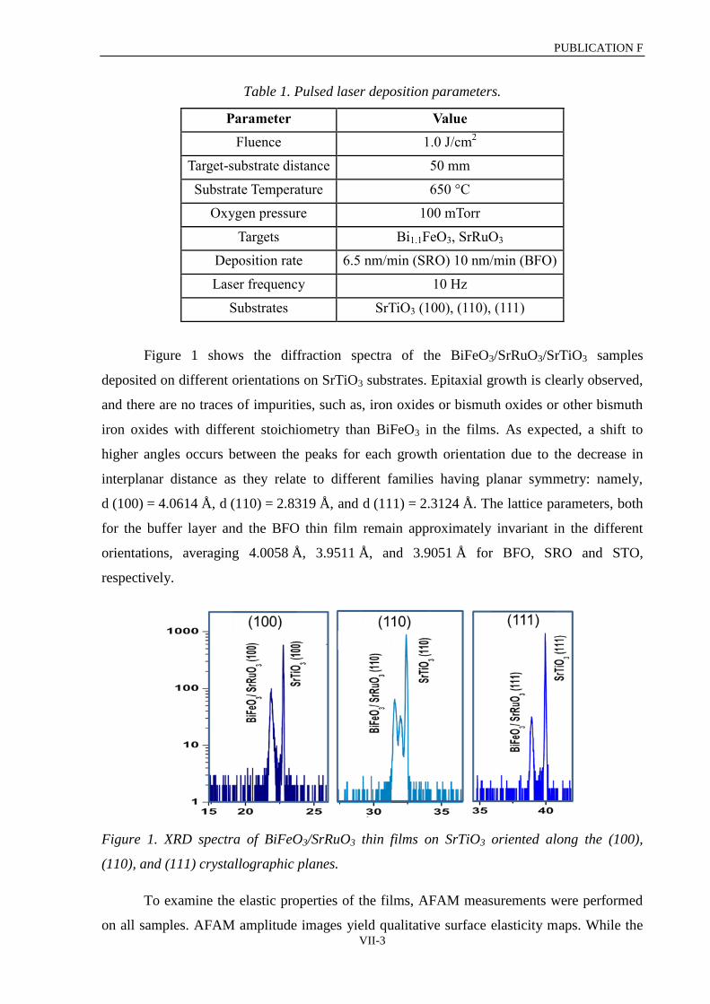
PUBLICATION F
VII-3
Table 1. Pulsed laser deposition parameters.
Parameter Value
Fluence 1.0 J/cm2
Target-substrate distance 50 mm
Substrate Temperature 650 °C
Oxygen pressure 100 mTorr
Targets Bi1.1FeO3, SrRuO3
Deposition rate 6.5 nm/min (SRO) 10 nm/min (BFO)
Laser frequency 10 Hz
Substrates SrTiO3 (100), (110), (111)
Figure 1 shows the diffraction spectra of the BiFeO3/SrRuO3/SrTiO3 samples
deposited on different orientations on SrTiO3 substrates. Epitaxial growth is clearly observed,
and there are no traces of impurities, such as, iron oxides or bismuth oxides or other bismuth
iron oxides with different stoichiometry than BiFeO3 in the films. As expected, a shift to
higher angles occurs between the peaks for each growth orientation due to the decrease in
interplanar distance as they relate to different families having planar symmetry: namely,
d (100) = 4.0614 Å, d (110) = 2.8319 Å, and d (111) = 2.3124 Å. The lattice parameters, both
for the buffer layer and the BFO thin film remain approximately invariant in the different
orientations, averaging 4.0058 Å, 3.9511 Å, and 3.9051 Å for BFO, SRO and STO,
respectively.
Figure 1. XRD spectra of BiFeO3/SrRuO3 thin films on SrTiO3 oriented along the (100),
(110), and (111) crystallographic planes.
To examine the elastic properties of the films, AFAM measurements were performed
on all samples. AFAM amplitude images yield qualitative surface elasticity maps. While the

PUBLICATION F
VII-4
sample surface is scanned, the AFM cantilever is excited to vibrate at a fixed ultrasonic
frequency close to a contact resonance. The cantilever vibration amplitude, and thus the
AFAM image contrast, depends on the difference between the excitation frequency and the
local contact resonance. The measurements were made with Pt-Ir coated tips (Nanosensors
PPP-EFM, Neuchâtel, Switzerland) with the free resonance of the first bending mode around
70 kHz. A representative AFAM image along with the topographic AFM image of the
BFO (100) sample are presented in Figure 2. The bright spots on Figure 2 are inclusions and
are common in PLD prepared thin films.
Figure 2. a) Topography and b) AFAM images from the BFO (100) sample at a frequency of
320 kHz, close to the contact resonance of the first bending mode of the cantilever. The elastic
properties of the film are homogeneous with exception of the inclusions (bright contrast on
the topography image).
The PFM experiments were performed using two different approaches: the
conventional low frequency, in which the excitation frequency is well below the resonances
of the cantilever, and the UPFM mode with excitation close to the contact resonance of the
first bending mode of the cantilever which enhance the piezo-mode signal through resonance
amplification [10]. Experiments done at the Technische Universität Hamburg-Harburg
(TUHH) were carried out on a VEECO Dimension 3100 AFM with a Nanoscope IV
controller, while a VEECO Dimension 3000 with a Nanoscope IIIA controller was used at
Fraunhofer IZFP. Pt-Ir coated probes were used for all measurements. For the conventional
PFM an excitation frequency of 10 kHz with amplitude of 3-5 V was applied to the tip. For
the UPFM an excitation frequency around 320 kHz with an amplitude of 4 V was applied to
the tip. In order to confirm ferroelectricity, poling experiments were carried out by applying a
DC voltage to the tip while the bottom electrode (SRO) was grounded. In this way, the
ferroelectric film below the tip switches its polarization direction. This method was applied to
films with the three different growth directions and using both conventional PFM and UPFM,

PUBLICATION F
VII-5
for simplicity only selected images are shown is this work. In all films the presence of small
amounts of inclusions was detected.
The images after the switching experiment with +22 V along with the topographic
image for the BFO (110) sample are shown in Figure 3. The lateral components of the two
polarization variants [4,5] are clearly observed in Fig. 3c, where the scanning (horizontal)
direction is parallel to the <110> direction. The inclusions, visible as the bright spots in the
topography image, do not show any piezoactivity and are visible in the VPFM and LPFM
Signals as spots with color corresponding to 0 V.
Figure 3. a) Topography, b) Vertical PFM (VPFM), and c) Lateral PFM (LPFM) of
ferroelectric domains written on BFO (110) film by applying +22 V DC while scanning over
a 3 x 3 m2 area of the sample. The polarization direction clearly changes (dark contrast) in
the VPFM image and the LPFM image.
In the case of the BFO (111) sample, no lateral component of the PFM signal is
expected. Figure 4 shows the results of the switching experiments for this sample. The first
square was switched by applying +22 V over an area of 2 x 2 µm2 and creates a dark contrast
in the VPFM image. For the second switching, a voltage of -22 V was applied over an area of
1 x 1 µm2 within the previously polarized area. The second switching led to a reversal of the
polarization direction to the initial condition. For both samples the PFM signals were stable
for up to 8 hours after the switching experiments; indicating that the expected quality of the
film and behavior of the domain structure was achieved. The single- (mono-) domain state of
the films can be explained by the strain in the films induced by the substrate as previously
reported [1].

PUBLICATION F
VII-6
Figure 4. a) Topography and b) Vertical PFM images of ferroelectric domains written on
BFO (111) film by applying +22 V DC while scanning over a 2 x 2 m2 area of the sample
followed by an applied DC voltage of -22 V while scanning over a 1 x 1 m2 area within the
already polarized area.
The BFO (100) sample is grown in a favorable direction for the visualization of the
domain structure; therefore, it does not need local switching of the polarization direction in
order to visualize the domains. Figure 5 shows the amplitude and phase signals of the vertical
and lateral UPFM measurements for this sample. The UPFM images were recorded with a
frequency close to the contact resonance (320 kHz) of the first bending mode of the
cantilever. The observed striped domain structure correlates very well with other reports in
the literature [1,4,12]. This indicates that the BFO (100) sample is of high quality and has the
expected domain structure.
Finally, in order to quantify the piezoelectric activity of the BFO (100) sample, the
PFM system was used to measure the deflection on the cantilever at different applied
voltages. Figure 6 presents the measured data and the linear fit which yields
d33 = 39 ± 2 pm/V. This value is in line with those from literature: d33 = 30-50 pm/V [1,12].

PUBLICATION F
VII-7
Figure 5. UPFM signals from BFO (100) film: Vertical UPFM a) amplitude and b) phase;
Lateral UPFM c) amplitude and d) phase. The domain structure is visible without local
switching.
Figure 6. Piezoelectric constant d33 measured using the PFM system.

PUBLICATION F
VII-8
3. CONCLUSIONS
We successfully grew high quality bismuth ferrite (BFO) epitaxial thin films on (100),
(110) and (111)-oriented SrRuO3/SrTiO3 substrates. The quality of the films was evaluated by
XRD confirming the epitaxial orientation of the films and the absence of second phases. PFM
and UPFM showed that the (111) and (110) oriented films are ferroelectric but are in a
monodomain state and that the (100) film shows a striped domain structure, as already
reported in the literature. The evaluation of the d33 piezoelectric constant for the (100) film
yields a value of d33 = 39 ± 2 pm/V, which is also in agreement with values already published
in the literature. AFAM measurements showed the homogeneity of the elastic properties of all
films.
REFERENCES
[1] N.A. Hill, Journal of Physical Chemistry B 104 (2000) 6694-6709.
[2] J. Wang, J. B. Neaton, H. Zheng, et al., Science 299 (2003) 1719.
[3] G. Catalan and J. F. Scott, Advanced Materials 21 (2009) 2463.
[4] R Ramesh, N.A. Spaldin, Nature Materials 6 (2007) 21-29.
[5] S.K Singh, H. Ishiwara, K. Maruyama, Journal of Applied Physics 100 (2006) 64102-
64105.
[6] Y. Chu, M.P. Cruz, C. Yang, et al., Advanced Materials 19 (2007) 2662-2666.
[7] Y. Chu, Q. Zhan, L.W. Martin, et al., Advanced Materials 18 (2006) 2307-2311.
[8] T. Zhao, A. Scholl, F. Zavaliche, et al., Nature Materials 5 (2006) 823-829
[9] A. Gruverman, O. Auciello, and H. Tokumoto, Annual Review of Materials Science 28
(1998) 101.
[10] U. Rabe, M. Kopycinska, S. Hisekorn et al., Journal of Applied Physics D: Applied
Physics 35 (2002) 2621.
[11] U. Rabe, K. Janser, W. Arnold, Review of Scientific Instruments 67 (1996) 3281-3293.
[12] F. Zavaliche, S.Y. Yang, T. Zhao, et al., Phase Transitions 79 (2006) 991-1017.

VII-1


PUBLICATION G
VIII-1
VIII. CHARACTERIZATION OF MATERIAL PROPERTIES AND
FUNCTIONALITIES OF LEAD-FREE BISMUTH-BASED CERAMICS
(PUBLICATION G)
L. Batista, U. Rabe, S. Hirsekorn
Part of the FP7-NMP-2010 EU-Mexico BisNano 263878 report, workpackage 9 (WP9),
January (2014).
ABSTRACT. Ferroelectric materials are widely used in many applications as sensors,
actuators, transducers, and memories. Most of these materials are however based on toxic
elements, as e.g. lead (Pb), which can create hazards during materials processing and also
disposal. With the new European regulations restricting the use of such toxic elements, the
need arises for new materials which provide the same or better functional properties. These
properties such as piezoelectric constants and high electromechanical coupling factors are
mostly determined by the microstructure and the arrangement of the ferroelectric domains. In
the framework of a European-Mexican project, lead-free Bismuth-based bulk ceramics like
Bi0.5Na0.5TiO3 (BNT), 0.94Bi0.5Na0.5TiO3-0.06BaTiO3 (BNT-BT), Mn-doped BNT-BT, and
Sr-doped BNT-BT were investigated and evaluated by different operating modes of an atomic
force microscope (AFM), especially dynamic modes in the ultrasonic range such as atomic
force acoustic microscopy (AFAM) and ultrasonic piezoelectric force microscopy (UPFM).
Macroscopic properties of the above mentioned lead-free, bismuth-based, polarized bulk
samples were also examined. Their piezoelectric activity was characterized by impedance and
3D laser vibrometer measurements. Mechanical properties such as Young’s and shear moduli
were determined by measuring longitudinal and transverse sound wave velocities and the
density. Using these data and the geometrical parameters of the samples, the first thickness
and radial resonance frequencies were calculated and compared to experimental spectra. In
the end, the most promising lead-free ceramic samples were then successfully tested as
ultrasonic transducer materials.

PUBLICATION G
VIII-2
1. INTRODUCTION
The work presented in this chapter is a part of the FP7-NMP-2010 EU-Mexico
BisNano 263878 report, workpackage 9 (WP9). The general objective of the BisNano
project [1] is the acquisition of fundamental knowledge on bismuth-based nanostructures, as a
new class of materials towards the development of value-added bismuth-based products and
devices. One of the specific objectives, which is included in WP9, is the evaluation of the
functionalities of the bismuth-based materials for a variety of applications, as e.g. lead (Pb)-
free piezoelectrics.
In this context, lead-free bulk ceramic samples from different partners (UPJV,
CINVESTAV and TUHH, see Table 1) have been sent to IZFP for materials characterization,
in WP9 especially for piezo-response characterization.
Table 1. BisNano partners who worked with IZFP in WP9.
Institution Location
Université de Picardie Jules Verne (UPJV) Amiens, France
Centro de Investigación y Estudios Avanzados (CINVESTAV) Querétaro, Mexico
Technische Universität Hamburg-Harburg (TUHH) Hamburg, Germany
2. BULK SAMPLES FROM UPJV AND COMMERCIAL REFERENCE MATERIAL
In order to characterize the macroscopic piezoelectric and elastic properties of the
lead-free bulk ceramic samples produced in our consortium, impedance, 3D laser vibrometer
and ultrasound measurements were performed. The samples were coated with electrodes if
necessary and polarized. Impedance measurements before and after polarization showed
whether the samples were macroscopically active. Using a laser vibrometer, the resonance
frequencies of the samples were detected, and the maximal surface vibration amplitudes were
measured quantitatively.
A bulk BNT sample and a bulk BNT-BT sample (circular plates with a thickness of
2.8 mm and 2.7 mm, and a diameter of 12 mm and 11.1 mm, respectively, were provided by
UPJV. The composition of the investigated materials is shown in Table 2.
Table 2. Composition of the investigated lead-free ceramic samples.
Abbreviation Chemical composition
BNT (Bi0.5Na0.5)TiO3
BNT-BT 0.94(Bi0.5Na0.5)TiO3-0.06BaTiO3

PUBLICATION G
VIII-3
The sample surfaces were sputtered with a thin gold electrode layer. By means of
impedance measurements no activity was found for both samples (Figs. 1a and b) in their
initial not polarized state.
Figure 1. Impedance measurements on the samples (a) BNT and (b) BNT-BT in their initial
state before polarization.
Then, in order to polarize the samples, a DC voltage of 7.5 kV was applied first at the
BNT-BT sample. It was interrupted after 2 min because of extreme heating of the sample.
Nevertheless, the sample showed very small piezoelectric activity (Fig. 2) after this
polarization. In order to avoid the heating, both samples were immersed in an electronic fluid
(3M Fluorinert FC-770) which cooled the samples.
Figure 2. Impedance measurements on the sample BNT-BT polarized by 7.5 kV during
2 minutes.
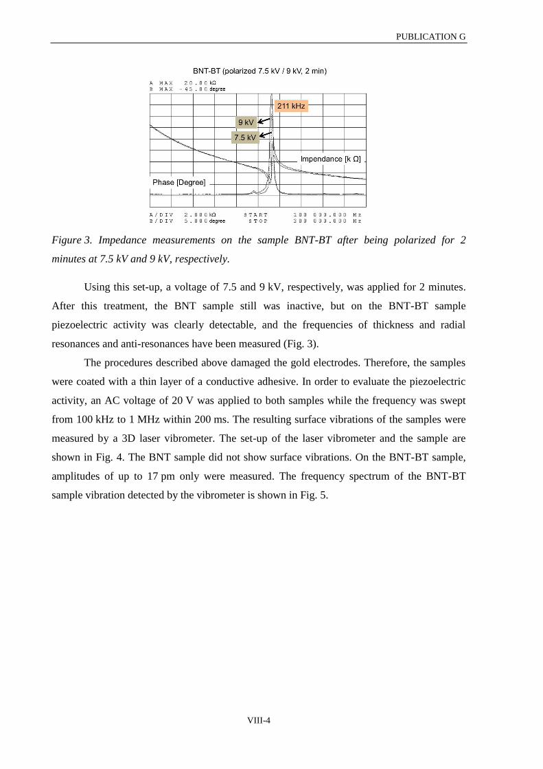
PUBLICATION G
VIII-4
Figure 3. Impedance measurements on the sample BNT-BT after being polarized for 2
minutes at 7.5 kV and 9 kV, respectively.
Using this set-up, a voltage of 7.5 and 9 kV, respectively, was applied for 2 minutes.
After this treatment, the BNT sample still was inactive, but on the BNT-BT sample
piezoelectric activity was clearly detectable, and the frequencies of thickness and radial
resonances and anti-resonances have been measured (Fig. 3).
The procedures described above damaged the gold electrodes. Therefore, the samples
were coated with a thin layer of a conductive adhesive. In order to evaluate the piezoelectric
activity, an AC voltage of 20 V was applied to both samples while the frequency was swept
from 100 kHz to 1 MHz within 200 ms. The resulting surface vibrations of the samples were
measured by a 3D laser vibrometer. The set-up of the laser vibrometer and the sample are
shown in Fig. 4. The BNT sample did not show surface vibrations. On the BNT-BT sample,
amplitudes of up to 17 pm only were measured. The frequency spectrum of the BNT-BT
sample vibration detected by the vibrometer is shown in Fig. 5.

PUBLICATION G
VIII-5
Figure 4. Set-up for the 3D laser vibrometer measurements.
Figure 5. Frequency spectrum obtained by laser vibrometer measurement on the sample
BNT-BT. Resonances were detected at 213 kHz and at 727 kHz as indicated in the figure.
As a reference, bulk lead-free piezoelectric ceramic samples from a commercial
company have been ordered by IZFP (circular plates with a thickness of 1 mm and a diameter
of 10 mm, coated with electrodes, PIC 700, PI Ceramic GmbH, Lederhose, Germany). The
ceramic samples are based on Bismuth Sodium Titanate (BNT) and are still at a laboratory
production level. The piezoelectric activity of these samples was checked by means of
impedance measurements and 3D laser vibrometer. The results were compared with a
standard PZT sample (PZ 29, Ferroperm Piezoceramics A/S, Kvistgard, Denmark) and with
the results from the bulk ceramic sample BNT-BT received from UPJV. The objective was to

PUBLICATION G
VIII-6
compare the macroscopic piezoelectric activity of a commercial lead-free piezoelectric
ceramic sample with the samples produced in our consortium.
Figure 6. Impedance measurements on the commercial lead-free piezoceramic PIC 700.
Figure 7. Impedance measurements on the commercial lead-free piezo-ceramic PIC 700
(continuous line) and on a standard PZT (PZ 29) from Ferroperm Piezoceramics A/S (dotted
line).
Figure 6 shows the impedance curve of a PIC 700 sample. It is macroscopically active
displaying impedance maxima at 251 kHz and 628 kHz. In order to compare the activity of
the PIC 700 sample with a standard PZT, the impedance curves of both samples were plotted
in Fig. 7. The PZT sample shows a much larger activity. The piezoelectric coupling factors of
BNT and BNT-BT components are lower than those of conventional PZT materials.

PUBLICATION G
VIII-7
3. BULK SAMPES FROM CINVESTAV AND TUHH
Further bulk samples were produced in the BisNano consortium, BNT-BT and Mn-
doped BNT-BT were provided by CINVESTAV and Sr-doped BNT-BT was provided by
TUHH. These samples were the most promising bulk lead-free piezoelectric materials for
ultrasonic transducer applications. The commercial lead-free ceramic PIC 700 mentioned in
the previous chapter was taken for comparison. The composition of the investigated materials
is shown in Table 3.
Table 3. Composition of the investigated lead-free ceramic samples.
Abbreviation Chemical composition
BNT-BT 0.94(Bi0.5Na0.5)TiO3-0.06BaTiO3
Mn-doped BNT-BT or BNT-BT +
0.005Mn or BNT-BT-Mn
0.995(0.94(Bi0.5Na0.5)TiO3-0.06BaTiO3)-
0.005Mn
Sr-doped BNT-BT or BNT-BT-ST or
BNT-BT-Sr
(0.85(Bi0.5Na0.5)TiO3-0.12BaTiO3-
0.03SrTiO3)
3.1 Macroscopic measurements with the bulk samples from CINVESTAV and TUHH
For the samples in Table 3, the bulk ultrasound longitudinal and transverse wave
velocities were measured at a frequency of 5 MHz. The Young’s (E) and the shear (G) moduli
were determined from the measured densities and sound velocities, the first thickness and
radial resonances of the samples were calculated from the sound velocities and the
geometrical parameters (Table 4). The results indicate that the Sr-doped BNT-BT (BNT-BT-
Sr) sample has the highest E and G moduli. The direct comparisons of elastic properties
should be carefully analyzed since the samples have different densities, which also influence
the elastic properties. Thus the results may be misinterpreted.
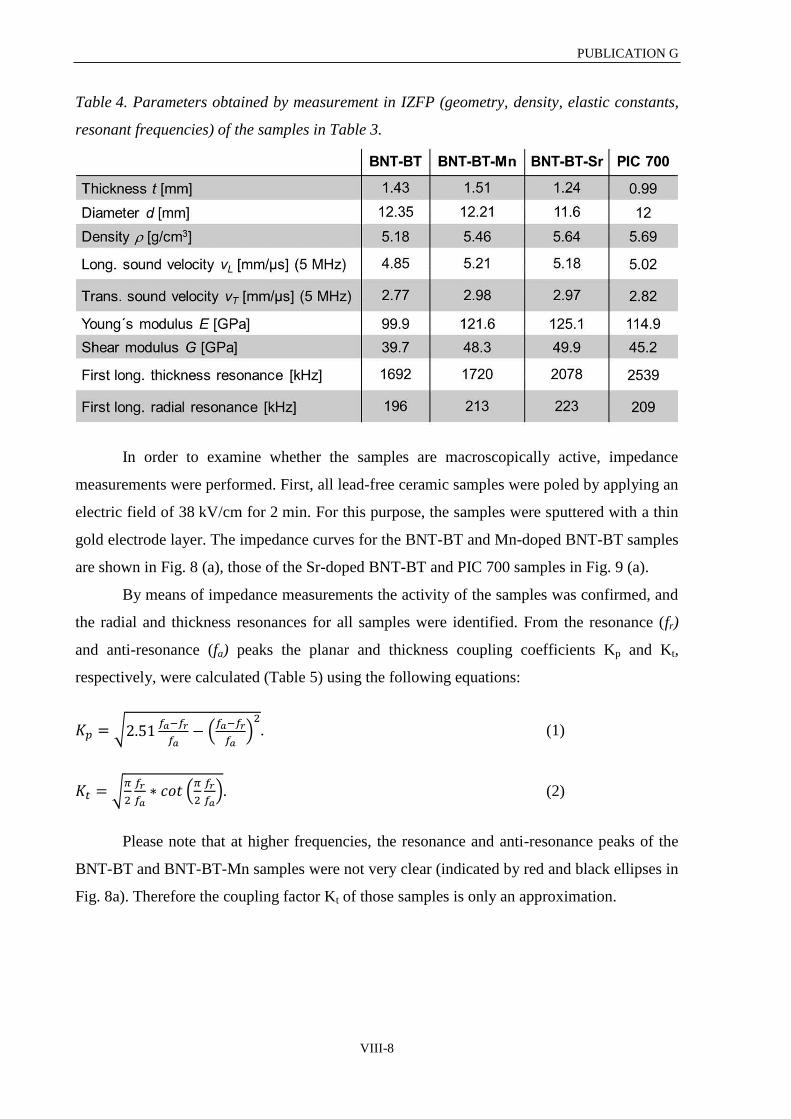
PUBLICATION G
VIII-8
Table 4. Parameters obtained by measurement in IZFP (geometry, density, elastic constants,
resonant frequencies) of the samples in Table 3.
In order to examine whether the samples are macroscopically active, impedance
measurements were performed. First, all lead-free ceramic samples were poled by applying an
electric field of 38 kV/cm for 2 min. For this purpose, the samples were sputtered with a thin
gold electrode layer. The impedance curves for the BNT-BT and Mn-doped BNT-BT samples
are shown in Fig. 8 (a), those of the Sr-doped BNT-BT and PIC 700 samples in Fig. 9 (a).
By means of impedance measurements the activity of the samples was confirmed, and
the radial and thickness resonances for all samples were identified. From the resonance (fr)
and anti-resonance (fa) peaks the planar and thickness coupling coefficients Kp and Kt,
respectively, were calculated (Table 5) using the following equations:
√
(
) . (1)
√
(
). (2)
Please note that at higher frequencies, the resonance and anti-resonance peaks of the
BNT-BT and BNT-BT-Mn samples were not very clear (indicated by red and black ellipses in
Fig. 8a). Therefore the coupling factor Kt of those samples is only an approximation.

PUBLICATION G
VIII-9
Figure 8. (a) Frequency plot of the electrical impedance and phase angle for the BNT-BT and
Mn-doped BNT-BT samples. (b) Laser vibrometer measurement on the BNT-BT and Mn-
doped BNT-BT samples showing clearly the amplitude vibrations at their respective
resonances.
Figure 9. (a) Frequency plot of the electrical impedance and phase angle for the Sr-doped
BNT-BT and PIC 700 samples. (b) Laser vibrometer measurement on the Sr-doped BNT-BT
and PIC 700 samples showing clearly the amplitude vibrations at their respective resonances.
The impedance curves reveal that the Sr-doped BNT-BT and the commercial PIC 700
samples show much higher resonance and anti-resonance peaks at higher frequencies than the
BNT-BT and Mn-doped BNT-BT samples.
Using the 3D laser vibrometer, the radial and thickness resonances of all samples were
again identified. An AC voltage of 20 V was applied while the frequency was swept from
100 kHz to 3 MHz within 10 ms. Fig. 8 (b) shows the amplitude versus frequency plot for the
BNT-BT and Mn-doped BNT-BT samples, and Fig. 9 (b) shows the amplitudes of the Sr-

PUBLICATION G
VIII-10
doped BNT-BT sample and the PIC 700 sample. The first radial and thickness resonances of
all samples are indicated in the figures. The results for the radial and thickness resonances
using calculations based on bulk ultrasonic velocities (Table 4), impedance and the laser
vibrometer (Figs. 8 and 9) measurements are in a good agreement.
Figure 10. Local surface displacement obtained by laser vibrometry measurements on the
BNT sample. An AC voltage of 1749 kHz frequency was applied. The images show the surface
displacement at the negative maximum (a) -20 V and at the positive maximum (b) 20 V of the
AC voltage.
Figure 11. Local surface displacement obtained by laser vibrometry measurements on the
Mn-doped BNT-BT sample at (a) -20 V and (b) 20 V. An AC voltage of 1593 kHz frequency
was applied.

PUBLICATION G
VIII-11
Figure 12. Local surface displacement obtained by laser vibrometry measurements on the Sr-
doped BNT-BT sample at (a) -20 V and (b) 20 V. An AC voltage of 1935 kHz frequency was
applied.
Figure 13. Local surface displacement obtained by laser vibrometry measurements on
PIC 700 sample at (a) -20 V and (b) 20 V. An AC voltage of 2269 kHz frequency was applied.
In order to measure the maximal surface vibration amplitudes, the samples were
scanned at their respective thickness resonance frequencies using again the laser vibrometer
technique. All measurements were performed by applying an AC voltage of 20 V. Figure 10
shows the laser vibrometer displacement measurements on the BNT-BT sample at 1749 kHz.
The maximal vibration amplitude measured close to the center point of the sample yields
6 nm. On Mn-doped BNT-BT the laser vibrometer displacement measurements show at
1593 kHz a 14 nm amplitude (Fig. 11). The same measurements were performed on the Sr-
doped BNT-BT and the PIC 700 samples as shown in Figs. 12 and 13, respectively. On the
Sr-doped BNT-BT sample the measurement was performed at 1935 kHz, on the PIC 700 at

PUBLICATION G
VIII-12
2269 kHz. The maximal vibration amplitudes are similar for both samples (about 18 nm). The
summary of the results can be found in Table 5.
Table 5. Summary of the measured properties using laser vibrometry and impedance
techniques.
3.2 Scanning probe measurements with the bulk materials from CINVESTAV and
TUHH
In addition to the macroscopic measurements, IZFP used micro- and nanoscopic
techniques to characterize the bulk samples provided by the project partners. In order to
investigate the micro- and nanoscopic piezoelectric properties of the lead-free bulk ceramic
samples produced in our consortium, AFM, AFAM and UPFM measurements were
additionally performed. The surface of the samples was carefully prepared using standard
polishing procedures. At IZFP, the PFM (Piezoresponse Force Microscopy) is combined with
ultrasonic techniques enabling the piezo-mode signal being enhanced through resonance
amplification. This technique is called Ultrasonic Piezoresponse Force Microscopy
(UPFM) [2]. The AFM, AFAM and UPFM investigations were performed using an Electrical
Force Microscopy (EFM)-cantilever (silicon cantilever coated with a Pt/Ir layer, PPP-EFM,
NanoWorld AG, Neuchâtel, Switzerland). The static spring constant of this type of cantilever
is in the range of 1-5 N/m. Prior to the AFAM and UPFM investigations the conventional
AFM contact mode was used to examine the surface topography of the sample surfaces, their
roughness and cleanness. The topography mode is furthermore active simultaneously to the
ultrasonic operation modes. Additional ultrasonic equipment is used in combination with the
commercial AFM for the AFAM and UPFM modes (chapter I, section 2 and 3). AFAM
amplitude images yield qualitative surface elasticity maps. In the UPFM mode, either
amplitude or phase images are taken for information about the sample’s piezo activity.

PUBLICATION G
VIII-13
Qualitatively, an increased contrast in the UPFM amplitude image corresponds to an
increased piezo activity. Similar to the vertical and lateral low frequency PFM modes, a
vibration of the cantilever in bending mode vertical to the sample surface corresponds to out-
of-plane sample surface activity (vertical UPFM), while a torsional vibration of the cantilever
corresponds to an in-plane sample surface activity (lateral UPFM). In this work, only UPFM
was performed. The ferroelectric properties of the samples were further examined by local
polarization experiments. A DC voltage of variable amplitude and poling direction was
applied between the tip and the sample while the sample surface was scanned. Afterwards the
same area was imaged in the UPFM mode to see whether the PFM contrast was changed
locally. The negative or positive DC voltage was increased stepwise from 5 V to 20 V until
the domain writing was successful. The first free flexural frequency of the type of cantilever
used here is found in the frequency range of 50-100 kHz and the corresponding first flexural
contact resonance frequency is found in the frequency range of 300-700 kHz.
Figure 14 (a) shows the contact-mode topography image of the BNT-BT bulk sample
produced by CINVESTAV. The vertical UPFM amplitude image is shown in Fig. 14 (b).
Very fine ferroelectric domains are observed mostly close to grain boundaries. In order to
confirm ferroelectricity of the BNT-BT bulk sample local switching experiments were
performed as shown in the vertical UPFM amplitude and phase images, respectively. The
switching experiment was performed by applying -20 V DC while scanning an area of 1.5 x
1.5 µm2 which created a dark contrast in the vertical UPFM amplitude and phase images
(Figs. 14 (c) and (d)). For the second switching, a voltage of +20 V DC was applied while
scanning an area of 0.5 x 0.5 µm2 within the same area which caused a reversal of the
polarization direction, i.e. a bright contrast (Figs. 14 (c) and (d)).

PUBLICATION G
VIII-14
Figure 14. Topography (a) and vertical UPFM amplitude image (b) of the BNT-BT bulk
sample. (c) and (d) show vertical UPFM amplitude and phase images, respectively, of
ferroelectric domains written in a selected grain of the sample by applying -20 V DC while
scanning over a 1.5 x 1.5 µm2 area of the sample followed by an applied DC voltage of +20 V
while scanning 0.5 x 0.5 µm2 within the same area (scan rate 2 Hz) [3].
Figure 15 (a) shows the topography image of the bulk Mn-doped BNT-BT sample also
produced by CINVESTAV. The vertical UPFM amplitude image is shown in Fig. 15 (b). A
higher piezo-activity is found in the center of the grains but no defined domain structure is
observed. Second-phase inclusions are detected on the grain boundaries as shown in the
topography image (Fig. 15 (c)). Those inclusions show no contrast in the UPFM amplitude
image (Fig. 15 (d)), and therefore, we may conclude that they do not show piezo-activity.

PUBLICATION G
VIII-15
Figure 15. Contact-mode topography (a) and vertical UPFM amplitude (b) images of the Mn-
doped BNT-BT bulk sample. Higher resolution contact mode topography (c) and vertical
UPFM amplitude (d) images show inclusions which do not show piezo-activity [3].
The bulk Sr-doped BNT-BT sample was produced by TUHH by sintering at 1150°C
for 2h. It has obtained 97% of the theoretically possible density. Macroscopic polarization and
strain curves were measured at TUHH (Ps ~ 40 μC/cm, Ec ~ 3 kV/mm, and d33 ~ 180 pm/V).
Contact-mode topography, UPFM, and AFAM images (Figs. 16 (a), (b) and (c)) were taken.
The topography in Fig. 16 (a) provides information about the microstructure and the surface
roughness. In Fig. 16 (b), the presence of ferroelectric domains is confirmed. Large domains
as well as very fine small domains (~ 20 nm) are observed. The AFAM image (Fig. 16 (c))
gives information of the elastic properties of the surface. Some grain and domain boundaries
which have different elastic properties compared to the grain interior are visible.

PUBLICATION G
VIII-16
Figure 16. Contact-mode topography (a), vertical UPFM amplitude (b) and AFAM (c) images
of the Sr-doped BNT-BT bulk sample. The images were recorded at a frequency of 324 kHz
close to the contact resonance of the first bending mode of the cantilever.
Figure 17. Contact-mode topography (a), vertical PFM images: (b) amplitude and (c) phase,
and AFAM (d) images of the Sr-doped BNT-BT bulk sample. The images were recorded at a
frequency of 332 kHz close to the contact resonance of the first bending mode of the EFM-
cantilever [3].

PUBLICATION G
VIII-17
Figure 17 shows another region of the Sr-doped BNT-BT sample. The topography
image (Fig. 17 (a)) reveals height differences which correspond to the large domains in the
UPFM image. Very fine ferroelectric domains are observed inside the large domains as shown
in the UPFM amplitude (Fig. 17 (b)) and phase (Fig. 17 (c)) images. The AFAM image
(Fig. 17 (d)) shows that the domain boundaries exhibit different elastic properties compared to
the interior of the domains.
We can summarize the macroscopic and the microscopic properties of the lead-free
bulk ceramic samples produced in our consortium as follows:
Macroscopic properties
- Sr-doped BNT-BT presents the highest E and G moduli.
- BNT-BT, Mn-doped BNT-BT, Sr-doped BNT-BT and PIC 700 become
piezoelectrically active after poling (38 kV/cm during 2 min).
- Using calculations based on bulk ultrasonic velocities, impedance, and laser
vibrometer measurements, the radial and thickness resonance frequencies of the
ceramic bulk samples were clearly identified.
- BNT-BT shows the lowest maximal vibration amplitude (6 nm). The Mn-doped BNT-
BT sample shows an intermediary maximal vibration amplitude (14 nm). The Sr-
doped BNT-BT and commercial PIC 700 samples show the largest maximal vibration
amplitudes (18 nm). The measurements were performed at the respective thickness
resonances of the samples by applying 20 V AC.
Microscopic properties
- BNT-BT shows grains with different piezo-activities. Some nano-domains close to the
grain boundaries were observed.
- Mn-doped BNT-BT shows higher piezo-activity in the center of the grains, no defined
domain structure was found. Second phase inclusions were characterized on the grain
boundaries, they do not present piezo-activity.
- Sr-doped BNT-BT displays large as well as very fine striped domains (~ 20 nm) over
the whole measured sample surface.
- Local polarization switching was possible in all bulk samples by applying -20 V DC
between the tip and the sample.

PUBLICATION G
VIII-18
4. CORRELATIONS
From all bulk lead-free ceramic samples produced in our consortium the Sr-doped
BNT-BT sample showed the most stable ferroelectric domain structure. The Mn-doped BNT-
BT sample presented an additional phase (inclusions) which do not show piezo-activity.
Macroscopic measurements using laser vibrometry showed that the Sr-doped BNT-BT sample
presents the largest surface vibration amplitudes. Hence, for ultrasonic transducer
applications, it is the most promising lead-free ceramic sample investigated in this work.
5. APPLICATIONS
Figure 18 (a) shows a set-up to test the most promising lead-free ceramic materials
produced in our consortium for ultrasonic transducer applications. A Polymethylmethacrylate
(PMMA) block with a thickness of 6 cm is used, on top of which the ceramic materials coated
with top and bottom electrodes and their respective electric contacts are glued. The thickness
of the PMMA block was chosen to be about twice the acoustic near-field length to avoid
interferences.
A standard ultrasonic pulse generator/receiver instrument was used for signal
excitation and reception. The generator sends a spike pulse with –125 V amplitude to the
transducer materials. All ceramic materials under test provided clear ultrasonic signals.
Examples of back wall echoes generated by the Mn- and Sr-doped BNT-BT samples,
respectively, are shown in Fig. 18 (b). The receiver amplification was set to 28 dB and 38 dB,
respectively. The normalized spectra of the received pulses are shown in Fig. 18 (c). The
spectrum of the spike signal used for excitation is also shown for comparison. The center
frequencies of the pulses generated by the BNT-BT-Mn and -Sr disks correspond well to the
resonance frequencies detected by laser vibrometry as presented in Figs. 11-13. Further
measurements are ongoing at IZFP to compare in detail the materials produced in this project
(Sr- and Mn-doped BNT-BT) to a commercial lead-free ceramic, PIC 700, and a standard lead
zirconate titanate ceramic material, PZ 29.

PUBLICATION G
VIII-19
Figure 18. Set-up used for ultrasonic testing of the lead-free piezoelectric ceramics produced
in this project (a). Ultrasonic pulses obtained using a conventional ultrasonic pulser/receiver
instrument in combination with the test set-up (b), Frequency spectra of the pulses (c).
REFERENCES
[1] EC-FP7 Call: NMP.2010.1.2-4 Adding Value to mining at the Nanostructure level,
Project: Functionalities of Bismuth-based nanostructures (BisNano) 263878.
[2] U. Rabe, M. Kopycinska, S. Hirsekorn, J. Muñoz-Saldaña, G.A. Schneider, W. Arnold,
Journal of Physics D: Applied Physics 35 (2002) 2621.
[3] M. Rank, Charakterisierung Bismut-basierter bleifreier Piezokeramiken mit Ultraschall-
Kraftmikroskopie und Ultraschall-Piezomode. Saarbrücken: Bachelor thesis, Science and
Technical Faculty III, Saarland University and IZFP report No. 130123-TW, 2013.


VIII-1


SUMMARY AND OUTLOOK
IX-1
IX. SUMMARY AND OUTLOOK
1. Structural steels
With the overall motivation to support the developments of nondestructive
electromagnetic and micromagnetic methods for material characterization and evaluation, the
first and larger part of this work explored and finally interpreted the micro- and nanoscopic
origin of the electromagnetic and micromagnetic output signals of one of the most extensively
studied material, pearlitic steel, by various SFM-electron microscopy combined studies. It
was shown that the detailed analysis of microstructural magnetic property relationships by
means of macroscopic magnetic measurements like hysteresis loop and MBN in combination
with micro- and nanoscopic imaging techniques like high resolution MFM and EBSD allows
a clear interpretation of magnetization processes in steels containing different phases
responsible for the macroscopic electromagnetic and micromagnetic measurement signals.
Samples of a high purity polycrystalline iron and of two unalloyed pearlitic steels
(Fe-0.8%C and Fe-1.5%C) containing globular cementite precipitates embedded in a ferrite
matrix were investigated. The samples were characterized macroscopically by measuring
hysteresis loops and MBN profiles. It was found that experimental conditions such as
magnetization frequency, magnetization amplitude, signal pick-up, band width, sample
surface condition, etc. play a crucial role on the measured results. Macroscopic magnetic
quantities like saturation magnetization, coercive field, and maximum Barkhausen noise
amplitude were measured and interpreted with respect to the microstructural state.
On the high purity iron sample large Barkhausen noise amplitudes were obtained at all
measured frequencies. This is attributed to the easy irreversible motion of domain walls
(mostly 180° BWs) in the annealed pure iron the microstructure of which presents low
densities of dislocations and lattice defects. In contrast, within the unalloyed pearlitic steel
samples, the 180° and 90° BWs in the ferrite interact with the cementite precipitates and with
the interstitial carbon atoms in the ferrite matrix. By optimizing the measured hysteresis loop
and MBN parameters the relative proportion and contributions of the cementite and ferrite
phases in the unalloyed pearlitic steels were determined. For the magnetic Barkhausen noise,
the choice of the frequency of the applied field plays a crucial role in the detection of the
cementite phase and the nondestructive evaluation of its proportion in unalloyed pearlitic
steels. At sufficiently high frequency (about 0.5 Hz), two peaks are observed. The observation
of two peaks in the MBN profiles of unalloyed pearlitic steels agrees with previous work [1]
performed at Fraunhofer IZFP.
SUMMARY AND OUTLOOK
IX-2
The behavior of the hysteresis loops and MBN measurement signals originate from the
underlying magnetic domains and their interactions with the microstructure. Most helpful in
correlating the macroscopic behavior with the microstructure and better understanding of the
above mentioned macroscopic measurement signals is the possibility to image the magnetic
micro- and nanostructure of macroscopic bulk (thick) sample surfaces. The magnetic
microstructures of the investigated samples and their dynamics were observed and
characterized using a magnetic force microscope. It was shown that the MFM technique not
only has a high spatial resolution and allows a relatively low cost implementation, but also
has a tremendous advantage for magnetic micro- and nanostructure imaging in steels because
local and collective magnetization switching behavior of large area scans (~ 100 m2) can be
recorded. The MFM was coupled with an external coil providing a controllable in-plane
magnetic field which allows the observation of the dynamic behavior of magnetic domains
and their interactions with the microstructure. It was shown that the choice of an appropriate
magnetic probe plays a crucial role on the quality and reliability of the MFM images. For the
samples studied in this work, the commercial CoCr coated probe (MESP) with a coating of
about 40 nm thickness showed the best contrast/resolution combination. The MESP probe did
not influence the magnetic microstructure of the investigated samples and vice-versa, and the
observed contrast clearly revealed the magnetic microstructure of the high purity iron and the
ferrite and cementite phases in the unalloyed pearlitic steel samples. Using the EBSD
technique, the crystalline orientation of both phases, cementite and ferrite, were determined
and correlated to the magnetic domain structure.
The domain arrangement at the surface is primarily determined by the principle of flux
closure which minimizes the total inner energy. Additionally, it is strongly dependent on the
orientation of the easy directions of the grains relative to the sample surface. In the simplest
case of pure iron, <001> is the easy direction, and therefore, a (100) surface contains two
mutually perpendicular easy directions. With increasing misoriention relative to the surface
till it contains no easy axis anymore, the domain patterns become progressively more
complicated. In order to observe domain wall dynamics (micromagnetic events) in the high
purity iron as well as in the ferrite phase of the unalloyed pearlitic steel samples, grains
oriented with its (100) plane in or close to the sample surface were chosen. In the high purity
iron sample, reversible and irreversible movements mainly of 180° domain walls were easily
demonstrated.
For the unalloyed pearlitic steel samples, the magnetic domain structure is more
complicated. The microstructure is composed of two phases, the soft ferromagnetic ferrite

SUMMARY AND OUTLOOK
IX-3
matrix and the cementite precipitates. An increasing amount of carbon in form of globular
cementite precipitates enhances the pinning of domain walls in the ferrite matrix due to the
presence of the second phase and its stress fields. Furthermore, the cementite phase increases
the magnetic hardness of steels because cementite is magnetically harder than ferrite. The
cementite precipitates have their own domain structure, and in order to reduce the
magnetostatic energy, spike domains are often formed at the interface between the two
phases. In general, the cementite precipitates showed a much stronger magnetic contrast than
the ferrite matrix. This is attributed to the stray fields which are stronger when emanating
from cementite compared to ferrite. Domain walls in the ferrite phase tend to intersect the
cementite precipitates in order to minimize the magnetostatic and wall energy, and they are
hindered in their movement by large and small precipitates. The wall width measured in the
ferrite phase ranges from 140 nm to about 500 nm, which is in the same order of magnitude as
the literature values, e.g. around 100 nm in iron. Analysis of MFM line scans across walls in
ferrite demonstrate average magnetic moments inside the walls either pointing out or into to
the surface plane.
Successively recorded MFM images with different strengths of the applied external
magnetic field elucidated reversible and irreversible break-free of domain walls in the ferrite
matrix from the cementite precipitates, which is interpreted as local Barkhausen events or
jumps. Measuring the curvature of a bowed 180° domain wall in the ferrite matrix
demonstrated the ability for local stress estimation. When an external magnetic field was
applied, the magnetization process in ferrite sets in already at low fields via the 180° and 90°
domain walls. In the ferrite matrix, 180° domain walls are mainly located in the center of
grains whereas 90° domain walls are mainly observed in connection with the closure domains
in the proximity of phase and grain boundaries. The activation of domain wall movements in
cementite required considerably stronger external fields, which is due to the high single
crystal anisotropy and the high density of defects (e.g. dislocations) and reflects the higher
magnetic hardness of cementite compared to ferrite. This microscopic observation correlates
qualitatively with the increase of magnetic hardness with increasing amount of cementite and
with the emergence of a second peak in the MBN signal due to the cementite phase at higher
external fields. The peak amplitude at the lower field corresponds to the amount of ferrite and
that one at the higher field to the amount of the cementite phase, respectively. This explains
the physical origin of the second peak in MBN profiles in unalloyed pearlitic steels containing
globular cementite in a ferrite matrix, which is discussed since years. The analysis of the
MFM images confirmed the observed macroscopic nondestructive electromagnetic signals.

SUMMARY AND OUTLOOK
IX-4
Contrary to the already existing data in the literature where the observation of domain wall
dynamics in steels required specially prepared (transparent to electrons) thin foils, it was
shown that also in macroscopic bulk (thick) samples, which are more relevant when
considering correlations with macroscopic NDT methods, domain wall dynamics can be
observed.
With the combination of MFM and EBSD techniques a new method to determine the
magnetic easy axes of micro- and nanoscopic ferromagnetic precipitates embedded in a bulk
material was demonstrated. Globular and lamellar cementite precipitates embedded in a ferrite
matrix in unalloyed steels were taken as examples. The MFM and EBSD techniques were
used for the visualization of the magnetic and crystallographic microstructures, respectively.
It was shown that the domain structures of cementite precipitates are strongly correlated to
their crystalline planes. MFM images with a local resolution down to 50 nm revealed
differently oriented magnetic moments in the cementite phase. The cementite domain
structure in a (010) crystal plane (at least almost) parallel to the sample surface, i.e. the long
easy [010]- or b-axis is (at least almost) perpendicular to this surface, was found to consist of
parallel stripes of strong opposite magnetic contrast. The magnetic moments of those
precipitates are positioned alternately down- and upwards perpendicularly to the surface and
are separated by 180° domain walls. The width of the domains at the sample surface is
dependent on the inclination of the (010) crystal plane relative to the surface and increases
with the angle between the easy [010] axis and the surface normal. The cementite precipitates
oriented with their (001) plane in or close to the surface plane showed a weak and
homogeneous contrast in the image leading to the conclusion that their magnetic moments are
oriented in-plane. By means of EBSD, the long [010]- or b-axis of these precipitates was
determined and correlated to the magnetic signal. Dark and bright imaged edges of the
precipitates confirmed the in-plane orientation of the magnetic moments along the long
[010]- or b-axis. The combined MFM and EBSD studies allow to conclude that the easy
direction of magnetization in cementite is the long [010]-axis. For the lamellar cementite
precipitates, the acquisition of EBSD patterns in order to determine their crystalline
orientation is very difficult. It was shown that the crystalline orientation of the cementite
lamellae can be estimated by simply imaging the magnetic and the topographic
microstructure.
The combined application of micro- and nanoscopic imaging techniques allowed a
correlation between microstructure and macroscopic material behavior and thus a better
understanding of the macroscopic electromagnetic NDT&E methods. Theoretical models

SUMMARY AND OUTLOOK
IX-5
based on microstructural magnetic property relationships in complex multiphase steels which
correlate the amount, size, and shape of precipitates, grain size and shape, etc. to important
macroscopic properties such as, for example, the magnetic hardness, can now be confronted
and developed by observing the microstructure and the magnetization dynamics directly on
the surface of macroscopic thick (bulk) samples. Additionally, parameters like depinning
fields, domain wall mobilities, etc. can be measured and used in micromagnetic simulation
software tools, e.g. 3D EMicroM [2], in order to study the evolution of macroscopic magnetic
signatures as function of changes in defect concentrations and/or the magnetic field.
Even though of high technological significance, the elastic constants of cementite are
still subject of debate. Atomic force acoustic microscopy was used to probe the local elastic
properties of the unalloyed steel samples with a spatial resolution down to 10 nm. Qualitative
AFAM surface elasticity maps indicated that in the measured area of the investigated
unalloyed Fe-0.8%C steel, ferrite is stiffer than cementite. To obtain quantitative elastic
moduli data, it is suggested to perform quantitative AFAM as well as nanoindentation
measurements on areas of each phase with known grain orientations. In this work,
topographic, magnetic, and elastic properties of the unalloyed pearlitic steel samples were
correlated.
Elastic properties of newly developed high strength steels were also investigated at the
nanoscale. AFAM, nanoindentation, and EBSD techniques were employed in order to
evaluate the local elastic properties as function of crystalline grain orientation of two different
austenitic twinning induced plasticity steels, Fe-22Mn-0.6C-0.2V and Fe-20Mn-3Si-3Al, with
average grain sizes of 1 μm and 40 μm, respectively. Even though the values measured using
nanoindentation were higher than those obtained by AFAM, the results from both techniques
presented the same trend, i.e. when comparing grains with similar crystalline orientations, the
steel Fe-22Mn-0.6C-0.2V showed higher stiffness than the steel Fe-20Mn-3Si-3Al, and for
both steels, the stiffness of grains in or around the (111) plane is higher than the stiffness of
grains in or around the (101) plane which is higher than the stiffness of grains in or around the
(001) plane. Finally, AFM contact mode was used to monitor local deformation behavior in
the Fe-22Mn-0.6C-0.2V steel. A series of topography images acquired for different plastic
deformation levels revealed an increase in step height with increasing plastic deformation,
which correlated with the formation of deformation twins, as was later confirmed by EBSD.

SUMMARY AND OUTLOOK
IX-6
2. Functional lead-free ferro- and piezoelectric ceramics
In the context of the European-Mexican collaborative project (BisNano) the objective
of which was the acquisition of fundamental knowledge on bismuth-based nanostructures
towards the development of products and devices, different lead-free bismuth based alloys
were synthesized in form of bulk samples as well as thin films in order to discover new lead-
free ferro- and piezoelectric materials for industrial applications.
Ferroelectric epitaxial thin films of bismuth ferrite (BiFeO3) were grown on (100),
(110) and (111)-oriented SrRuO3/SrTiO3 substrates. The thickness of the films varied between
100 and 200 nm. The quality of the films with regard to their epitaxial orientation and absence
of second phases were confirmed using XRD. AFM contact mode topography images showed
a flat surface (low range of the height scale, max. 33 nm). The homogeneity of the elastic
properties of all films was confirmed using AFAM. To study the influence of the
crystallographic orientation of the films on the ferroelectric domain patterns, low frequency
(standard) as well as ultrasonic piezoresponse force microscopy were used. By combining the
vertical and the lateral piezoresponse data, it was shown that the (111) and (110) oriented
films are ferroelectric, but are in a mono-domain state and that the (100) film presented a
striped domain structure. Local polarization switching was possible in all films by applying
22 V DC between the AFM tip and the sample. Analysis of the lateral PFM signal acquired on
the (110) and (111) oriented films after the polarization switching shows a lateral component
on the (110) film, but no contrast on the (111) film. The results are in accordance to the
literature data in which the (100), (110), and (111)-oriented films have 4-, 2-, and
1-polarization variants, respectively, because of the symmetry of the rhombohedrally distorted
perovskite BiFeO3 structure. Finally, the measurement of the d33 piezoelectric constant of the
(100) film with the PFM system yielded a value of d33 = 39 ± 2 pm/V. The high polarization
and piezoelectric response in thin BiFeO3 films suggest a possibly environmentally acceptable
alternative to Pb-based ferroelectrics. However, further comprehensive investigations of the
processes related to ferroelectric fatigue are still necessary. In addition, large ferroelectric
coercive field and high leakage currents are considered as further limitations in utilizing
BiFeO3 for commercial device applications.
Not only thin films, but also bulk ceramic samples were investigated. Promising
candidates for lead-free piezoelectric materials like Bi0.5Na0.5TiO3 (BNT),
0.94Bi0.5Na0.5TiO3-0.06BaTiO3 (BNT-BT), Mn-doped BNT-BT and Sr-doped BNT-BT were
synthesized in bulk form by different BisNano partners. A commercial lead-free ceramic
based on BNT, called PIC 700, was taken for comparisons. The samples were investigated

SUMMARY AND OUTLOOK
IX-7
and evaluated at different scales. The samples BNT-BT and Mn-doped BNT-BT provided by
the Centro de Investigación y Estudios Avanzados and Sr-doped BNT-BT provided by the
Technische Universität Hamburg-Harburg were the most promising bulk lead-free
piezoelectric materials produced in the BisNano consortium for industrial applications. The
density of the samples was measured using the so-called Archimedes method. The Sr-doped
BNT-BT and the PIC 700 samples exhibit the largest densities ( = 5.64 g/cm3 and
= 5.69 g/cm3, respectively), which corroborate the AFM topographic and optical images,
where much lower porosity levels were observed in these samples compared to the other ones.
Macroscopic mechanical and piezoelectric properties were characterized using
ultrasonic, impedance, and 3D laser vibrometer measurements. The bulk ultrasound
longitudinal and transverse wave velocities were measured at a frequency of 5 MHz.
Mechanical properties such as Young’s and shear moduli were determined by measuring
longitudinal and transverse sound wave velocities and the density. The sample Sr-doped
BNT-BT showed the largest Young’s and shear moduli (E = 125.1 GPa and G = 49.9 GPa,
respectively). Before the impedance and the 3D laser vibrometer measurements, the samples
were sputtered with a thin conductive electrode layer and poled by applying an electric field
of 38 kV/cm for 2 min. By means of impedance measurements the activity of the samples was
confirmed, and the radial and thickness resonances of all samples were identified. From the
resonance (fr) and anti-resonance (fa) peaks the planar and thickness coupling coefficients Kp
and Kt, respectively, were calculated. The sample Sr-doped BNT-BT presented the largest
thickness coupling coefficient (Kt = 0.37), whereas the sample PIC 700 showed the largest
planar coupling coefficient (Kp = 0.37). Using a laser vibrometer, the resonance frequencies
of the samples were detected, and the maximal surface vibration amplitudes measured at their
thickness resonances were obtained quantitatively. All measurements were performed by
applying an AC voltage of 20 V. The measured thickness resonance frequencies of all
samples ranged from 1749 to 2269 kHz. The maximal vibration amplitudes were measured
close to the center point of the samples. The BNT-BT sample showed the lowest maximal
vibration amplitude (6 nm), the Mn-doped BNT-BT sample displayed a medium maximal
vibration amplitude (14 nm), and the maximum in vibration amplitudes were found on the Sr-
doped BNT-BT and commercial PIC 700 samples, both samples yielded 18 nm.
The above mentioned macroscopic properties of the ceramic samples are mostly
determined by the microstructure and the arrangement of the ferroelectric domains. AFM was
used to image the surface micro- and nanostructures. Surface elastic properties and
ferroelectric domains were imaged at a nanoscale in all samples using AFAM and UPFM,

SUMMARY AND OUTLOOK
IX-8
respectively. Grains with different piezo-activities were observed on the BNT-BT sample, and
some nanodomains were detected close to the grain boundaries. The Mn-doped BNT-BT
sample showed higher piezo-activity in the center of the grains. However, no defined domain
structure was found. Additionally, second phase inclusions which did not present piezo-
activity were detected at the grain boundaries. A well-defined high-contrast domain structure
was observed on the Sr-doped BNT-BT sample. Large as well as very fine striped domains
(~ 20 nm) over the whole measured sample surface were detected. Local polarization
switching was possible by applying 20 V DC between the AFM tip and the sample.
Finally, the most promising lead-free bismuth-based bulk ceramic samples produced
in the BisNano consortium were successfully tested as ultrasonic transducer material. A
testing setup was built, and together with a conventional ultrasonic pulser/receiver instrument,
ultrasonic pulses were obtained. The results indicated that the Sr-doped BNT-BT sample
exhibited the best performance, which confirms the previously measured macroscopic and
micro- and nanoscopic properties, i.e. the Sr-doped BNT-BT sample presented the highest
density, the highest E- and G moduli, the largest thickness coupling coefficient, and the most
distinct and stable ferroelectric domain structure. Therefore, the Sr-doped BNT-BT material
has high potential to be applied in ultrasonic transducers as an alternative to lead-based
piezoelectric materials.
REFERENCE
[1] I. Altpeter, Spannungsmessung und Zementitgehaltsbestimmung in Eisenwerkstoffen
mittels dynamischer magnetischer und magnetoelastischer Meßgrößen, Dissertation, Saarland
University, Saarbrücken (1990).
[2] Stéphane Labbé and Pierre Leca, EMicroM, Simulation de l'évolution de l'aimantation
dans les matériaux ferromagnétiques, ONERA, numéro APP:
IDDN.FR.001.320023.R.P.1998.000.31235 (1998).

IX-9


LIST OF PUBLICATIONS
X-1
X. LIST OF PUBLICATIONS
Papers in Journals:
L. Batista, U. Rabe, S. Hirsekorn, “Magnetic micro- and nanostructures of unalloyed steels:
Domain wall interactions with cementite precipitates observed by MFM”, NDT & E
International 57 (2013) 58–68.
L. Batista, U. Rabe, I. Altpeter, S. Hirsekorn, G. Dobmann “On the mechanism of
nondestructive evaluation of cementite content in steels using a combination of magnetic
Barkhausen noise and magnetic force microscopy techniques”, Journal of Magnetism and
Magnetic Materials 254 (2014) 248–256.
L. Batista, U. Rabe, S. Hirsekorn, “Determination of the easy axes of small ferromagnetic
precipitates in a bulk material by combined magnetic force microscopy and electron
backscatter diffraction techniques”, submitted to Ultramicroscopy.
R. P. Fernandes, L. Batista, A.D.G. Castro, L. Salamanca-Riba, M.P. Cruz, J. Muñoz-Saldaña,
F. Espinoza-Beltran, S. Hirsekorn, U. Rabe, G.A. Schneider, “Piezoresponse force
microscopy studies on (100), (110) And (111) epitaxial growth of BiFeO3 thin films”, MRS
Proceedings 1477 (2012) doi:10.1557/opl.2012.1701.
M. Bousquet, L. Batista, J. L. Dellis, A. Boulle, U. Rabe, O. Durand-Drouhin, Y. Gagou, L.
Dupont, V. Viallet, A. Zeinert, S. Hirsekorn, N. Lemée, “Structural and electrical properties
of Bi0.5Na0.5 TiO3 based superlattices grown by pulsed laser deposition”, to be submitted to
Journal of Applied Physics.
Conferences:
L. Batista, U. Rabe, S. Hirsekorn, “Characterization of the magnetic micro- and
nanostructure in unalloyed steels by magnetic force microscopy”, Review of Progress in
Quantitative Nondestructive Evaluation (QNDE), 39th
Annual Meeting, 16th
-20th
July (2012),
Denver, Colorado, USA, Vol. 32, AIP Conference Proceedings 1511 (2013) 1180–1187.
L. Batista, U. Rabe, S. Hirsekorn, “Micro- and nanostructure characterization and imaging of
twip and unalloyed steels”, Review of Progress in Quantitative Nondestructive Evaluation
(QNDE), 38th
Annual Meeting, 17th
-22th
July (2011), Burlington, Vermont, USA, Vol.31, AIP
Conference Proceedings 1430 (2012) 1381–1388.
S. Hirsekorn, U. Rabe, L. Batista, L. Behl, “Microstructure characterization and imaging of
fine-grained steel by microscopic ultrasonic techniques”, Review of Progress in Quantitative
Nondestructive Evaluation (QNDE), 37th
Annual Meeting, 18th
-23th
July (2010), San Diego,
California, USA, Vol. 30A, AIP Conference Proceedings 1335 (2011) 1097–1103.
L. Batista, U. Rabe, S. Hirsekorn, “Cementite Content in Steel: Magnetic Barkhausen Noise
and Visualization of Domain Wall Movement by Magnetic Force Microscopy” (poster),
Symposium: Crackling noise and intermittency in condensed matter, 22th
–24th
May (2013),
Göttingen, Germany.

LIST OF PUBLICATIONS
X-2
U. Rabe, L. Batista, S. Hirsekorn, “Magnetic micro- and nanostructures of steels imaged by
magnetic force microscopy: Is it possible to observe a local Barkhausen jump?”, Symposium:
Crackling noise and intermittency in condensed matter, 22th
–24th
May (2013), Göttingen,
Germany.
L. Batista, U. Rabe, S. Hirsekorn, “Magnetic micro- and nanostructures of unalloyed steels
observed by magnetic force microscopy” (poster), Materials Science and Engineering (MSE),
25th
–27th
September (2012), Darmstadt, Germany.
L. Batista, U. Rabe, S. Hirsekorn, “Micro- and Nanostructure Characterization and Imaging
of TWIP and Unalloyed Steels”, "NDT in Progress", 10th
–12th
October (2011), Prague, Czech
Republic.
L. Batista, U. Rabe, S. Hirsekorn, “Darstellung von Mikro- und Nanostrukturen in
perlitischen Stählen mittels elektromagnetischer zfP-Verfahren” (in german), DGZfP-
Jahrestagung 6th
–8th
May (2013), Dresden, Germany.
L. Batista, U. Rabe, S. Hirsekorn, “Characterization of Lead-Free Bismuth-Based Ceramics
by Bulk Ultrasound and Ultrasonic Operation Modes of Atomic Force Microscopy” (poster),
EuroNanoforum (ENF), 18th
–20th
June (2013), Dublin, Ireland.
L. Batista, U. Rabe, S. Hirsekorn, “Micro- and Nanostructure Characterization Imaging of
TWIP Steels”, Deutsche Physikalische Gesellschaft (DPG-Jahrestagung) 13th
–18th
March
(2011), Dresden, Germany.
L. Batista, U. Rabe, S. Hirsekorn, M. Bousquet, N. Lemée, O. Durand-Drouhin, A. Zeinert,
E.J. Herrera-Jiménez, A.C. Garcia-Castro, F.J. Espinoza-Beltrán, J. Muñoz-Saldaña,
“Characterization of bismuth-based ceramics using bulk ultrasonics and ultrasonic modes of
atomic force microscopy”, XXI International Materials Research Congress (IMRC) 12th
–17th
August (2012), Cancún, Mexico.
L. Batista, U. Rabe, S. Hirsekorn, “Characterization and Investigation of Material Properties
and Functionalities of Bismuth-Based Nanostructures”, VI International Conference on
Surfaces, Materials and Vacuum (ICSMV) 23th
–27th
September (2013), Mérida, Mexico.
U. Rabe, L. Batista, S. Hirsekorn, “Application of Atomic Force Acoustic Microscopy and
Ultrasonic Piezoelectric Force Microscopy to Characterization of Bismuth-Based
Piezoelectric Ceramics”, IEEE International Ultrasonics Symposium (IUS), 21st–25
th July
(2013), Prague, Czech Republic.
L. Batista, U. Rabe, S. Hirsekorn, “Materialcharakterisierung und Anwendung von bleifreien
Keramiken auf Bismut-Basis” (in german), DGZfP-Jahrestagung 26th
–28th
May (2014),
Potsdam, Germany.
L. Batista, U. Rabe, S. Hirsekorn, “Investigation of the mechanical and piezoelectric
properties of Bismuth-based ceramics on the macro- and nanoscales”, Nanobrücken-
Nanomechanical Testing Workshop, 26th
–28th
March (2014), Saarbrücken, Germany.