Exact Solutions of Steady Thin Film Flows of Modified ...
10
J. Basic. Appl. Sci. Res., 4(11)71-80, 2014 © 2014, TextRoad Publication ISSN 2090-4304 Journal of Basic and Applied Scientific Research www.textroad.com *Corresponding Author: M. Farooq, Department of Mathematics, National University of Computer & Emerging Sciences, Peshawar, Pakistan. Email: [email protected] Exact Solutions of Steady Thin Film Flows of Modified Second Grade Fluid on a Vertical Belt M. T. Rahim 1 , M. Farooq 1* , S. Islam 2 , A. M. Siddiqui 3 , M. Ali 1 , Murad Ullah 4 1 Department of Mathematics, National University of Computer and Emerging Sciences, Peshawar, Pakistan. 2 Department of Mathematics, Abdul Wali Khan University, Mardan, Khyber Pakhtunkhwa, Pakistan. 3 Department of Mathematics, Pennsylvania State University, York Campus, 1031 Edgecomb Avenue, York, PA 17403, USA. 4 Department of Mathematics, Islamia College University, Peshawar, Pakistan Received: February 11, 2014 Accepted: October 29, 2014 ABSTRACT This paper explores the problem of thin film for two types of flows i.e., (i) lifting and (ii) drainage of a steady, incompressible, non-isothermal modified second grade fluid. Exact solutions are obtained for the modeled highly non-linear ordinary differential equations subject to suitable boundary conditions. The Newtonian solutions are retrieved for the flow behavior index m=0 [1]. Explicit expressions for velocity profile, temperature distribution, average velocity, volume flow rate and shear stress on the moving and stationary belt are obtained in both cases. It is observed from this study that the flow of thin films is strongly depending on m (flow behavior index of modified second grade fluid), t S (Stokes number) and r B (Brinkman number).Also the effects of various emerging parameters on the velocity and temperature of the fluid are presented graphically. KEYWORDS: Lifting, Drainage, Modified second grade fluid, Exact solution. 1. INTRODUCTION The fluids of non-Newtonian behavior are of great interest to researchers [1, 2, 17, 21-22] for their significance in industry and engineering sector. The Navier-Stokes equations are proved to be insufficient to depict and obtain the distinctiveness of complex rheological fluids as well as polymers [3]. A large amount of the industrial and biological fluids are of non-Newtonian nature. Honey, ketchup of tomato, blood, plastic, shampoo, certain oils and greases, paint, mud and polymer solutions are common examples of such fluids. In general non-Newtonian fluids show shear-thinning/shear-thickening behavior [4]. The meagerness of classical theories to explain such liquids has led to the growth of new theory to study fluids of non-Newtonian nature. It is a known fact that because of complexity of liquids, a single model cannot be used to describe the effects of all non-Newtonian fluids. For this reason several constitutive models have been proposed in fluid mechanics. Among these the differential type fluids have attained special status. A subclass of the fluids of the differential type is the modified second grade fluid, which have been deliberated successfully in a variety of flow situations. The non-linear response of these liquids constitutes a significant field of mathematical modeling. The governing equations of motion are highly non-linear and finding exact solutions is a difficult task. Thin film flows are very important due to their applications in engineering, biomedical, material processing and industries. Such applications include microchip production, lining of mammalian lungs. Many researchers have studied thin film flow to understand different types of its configuration. The flow of a thin film can be produced by various means; for instance gravity, thermal effects and configuration forces. The literature on thin film flows is extensive for viscous fluids [5], but no proper attention has been given to such problems involving non-Newtonian fluids. Few attempts [6 – 9, 14, 15] have been made which deal with the non-Newtonian thin film flows. In all these studies,the authors have either used the homotopy perturbation technique or the homotopy analysis method. There are very few cases, especially for the non-Newtonian fluids, in which the exact solutions of momentum equations were found. The study of heat transfer to a falling liquid layer has been a matter of broad research in the last few decades [10 – 13, 16]. In most of these studies, the power-law fluid model is taken as the non-Newtonian fluid. Only modest attention has been devoted to the studies where the effects of viscousdissipation areincorporated, althoughthis has been shown to be very significant in various cases such as polymer processing. 71
Transcript of Exact Solutions of Steady Thin Film Flows of Modified ...

J. Basic. Appl. Sci. Res., 4(11)71-80, 2014
© 2014, TextRoad Publication
ISSN 2090-4304
Journal of Basic and Applied
Scientific Research
www.textroad.com
*Corresponding Author: M. Farooq, Department of Mathematics, National University of Computer & Emerging Sciences, Peshawar, Pakistan. Email: [email protected]
Exact Solutions of Steady Thin Film Flows of Modified Second Grade Fluid
on a Vertical Belt
M. T. Rahim1, M. Farooq
1*, S. Islam
2, A. M. Siddiqui
3, M. Ali
1, Murad Ullah
4
1Department of Mathematics, National University of Computer and Emerging Sciences, Peshawar, Pakistan.
2Department of Mathematics, Abdul Wali Khan University, Mardan, Khyber Pakhtunkhwa, Pakistan.
3Department of Mathematics, Pennsylvania State University, York Campus, 1031 Edgecomb Avenue, York, PA
17403, USA. 4Department of Mathematics, Islamia College University, Peshawar, Pakistan
Received: February 11, 2014
Accepted: October 29, 2014
ABSTRACT
This paper explores the problem of thin film for two types of flows i.e., (i) lifting and (ii) drainage of a steady,
incompressible, non-isothermal modified second grade fluid. Exact solutions are obtained for the modeled highly
non-linear ordinary differential equations subject to suitable boundary conditions. The Newtonian solutions are
retrieved for the flow behavior index m=0 [1]. Explicit expressions for velocity profile, temperature distribution,
average velocity, volume flow rate and shear stress on the moving and stationary belt are obtained in both cases. It is
observed from this study that the flow of thin films is strongly depending on m (flow behavior index of modified
second grade fluid), t
S (Stokes number) andr
B (Brinkman number).Also the effects of various emerging
parameters on the velocity and temperature of the fluid are presented graphically.
KEYWORDS: Lifting, Drainage, Modified second grade fluid, Exact solution.
1. INTRODUCTION
The fluids of non-Newtonian behavior are of great interest to researchers [1, 2, 17, 21-22] for their
significance in industry and engineering sector. The Navier-Stokes equations are proved to be insufficient to depict
and obtain the distinctiveness of complex rheological fluids as well as polymers [3]. A large amount of the industrial
and biological fluids are of non-Newtonian nature. Honey, ketchup of tomato, blood, plastic, shampoo, certain oils
and greases, paint, mud and polymer solutions are common examples of such fluids. In general non-Newtonian
fluids show shear-thinning/shear-thickening behavior [4]. The meagerness of classical theories to explain such
liquids has led to the growth of new theory to study fluids of non-Newtonian nature. It is a known fact that because
of complexity of liquids, a single model cannot be used to describe the effects of all non-Newtonian fluids. For this
reason several constitutive models have been proposed in fluid mechanics. Among these the differential type fluids
have attained special status. A subclass of the fluids of the differential type is the modified second grade fluid, which
have been deliberated successfully in a variety of flow situations. The non-linear response of these liquids
constitutes a significant field of mathematical modeling. The governing equations of motion are highly non-linear
and finding exact solutions is a difficult task.
Thin film flows are very important due to their applications in engineering, biomedical, material processing
and industries. Such applications include microchip production, lining of mammalian lungs. Many researchers have
studied thin film flow to understand different types of its configuration. The flow of a thin film can be produced by
various means; for instance gravity, thermal effects and configuration forces. The literature on thin film flows is
extensive for viscous fluids [5], but no proper attention has been given to such problems involving non-Newtonian
fluids. Few attempts [6 – 9, 14, 15] have been made which deal with the non-Newtonian thin film flows. In all these
studies,the authors have either used the homotopy perturbation technique or the homotopy analysis method. There
are very few cases, especially for the non-Newtonian fluids, in which the exact solutions of momentum equations
were found.
The study of heat transfer to a falling liquid layer has been a matter of broad research in the last few
decades [10 – 13, 16]. In most of these studies, the power-law fluid model is taken as the non-Newtonian fluid. Only
modest attention has been devoted to the studies where the effects of viscousdissipation areincorporated,
althoughthis has been shown to be very significant in various cases such as polymer processing.
71
Farooq et al.,2014
Because of the nonlinearity of the Navier-Stokes equations, a small number of exact solutions are found in
literature. This is because of the nonlinearity in the inertial part and higher order in viscosity part. Numerical
solutions of differential equations, no matter how accurate, are still not exact solutions because the parameters
involved in equation have to be assigned values for each solution. Exact solutions are important for the following
reasons [18-20].
(i). These solutions represent fundamental fluid-dynamic flows. Also the basic phenomena described by the Navier-
Stokes equations can be studied more closely because of the uniform validity of exact solutions.
(ii). Exact solutions serve as accuracy checks for experimental, asymptotic and numerical or empirical methods.
Although computer techniques make the complete integration of the equation of motion feasible, the accuracy of the
results can be established by comparison with an exact solution.An excellent review of exact solutions of the
Navier-Stokes equation has been given by Wang [18].
In the present paper, we considered modified second grade fluid, and discussed the flow problems on a
vertically upward moving belt and down a stationary vertical belt. Exact solutions of the modeled nonlinear ordinary
differential equations subject to suitable boundary conditions, are achieved in both cases. Form=0, we recover
velocity of Newtonian case [5]. Expressions for velocity, temperature, volume flow rate, average velocity and shear
stress on the moving and stationary belt are also calculated. It is observed that for steady case, generalized
(modified) second grade fluid shows the results of power law model.
This paper is organized as follows: Section 2 presents basic equations for modified second grade fluid, Section
3 transforms equations in section 2 for lifting problem and obtains exact solutions for velocity profile and
temperature distribution. Section 4 calculates volume flux, average velocity and belt shear stress for lifting problem.
Section 5 used equations from section 2 for drainage problem and found exact solutions for velocity profile and
temperature distribution. Section 6 calculates volume flow rate, average velocity and shear stress on the belt for
drainage problem. Results and discussion are given in section 7 and conclusion is provided in section 8.
2. BASIC FLOW EQUATIONS
The basic equations governing the flow of an incompressible fluid including thermal effects are:
,0=⋅∇ V (1)
,TfV
⋅∇+∇−= pdt
dρρ (2)
,
2LT ⋅+Θ∇=
Θκρ
dt
dC
p (3)
whereV is the velocity vector, d
dt is the material time derivative defined as
( ) ( )**
∇⋅+
∂
∂= V
tdt
d,
ρ is the constant density, f is the body force, p is the dynamic pressure, Θ is the temperature, p
C is the specific
heat constant, κ is the thermal conductivity and T is the extra stress tensor which is defined differently for different
fluids. We choose the modified second grade fluid for our case. The extra stress tensor for such a fluid is given by
,
2
2 1211AAAT ααµ ++= eff (4)
where21
and αα are the normal stress coefficients, effµ is an effective viscosity for generalized second grade
fluid, and a function of the shear rate, defined as
,2
1 22
1
m
eff tr
= Aηµ
η is the flow consistency index and m is the flow behavior index. The RivlinEricksen tensors, 2
AA and1
are
defined as
72
J. Basic. Appl. Sci. Res., 4(11)71-80, 2014
.
,,
11
1
1
ALLAA
A
VLLLA
2
T
T
dt
d++=
∇=+=
For 0m < , the fluid is shear thinning, for 0m > the fluid is shear thickening and for 0m = we obtain second
grade fluid model. On the other hand, if 1 2
0α α= = , equation (4) reduces to the power-law model and for
021=== ααm , we obtain the classical Newtonian model. It is worth mentioning that the flow behavior index m
must have the limits 11 <<− m [13].
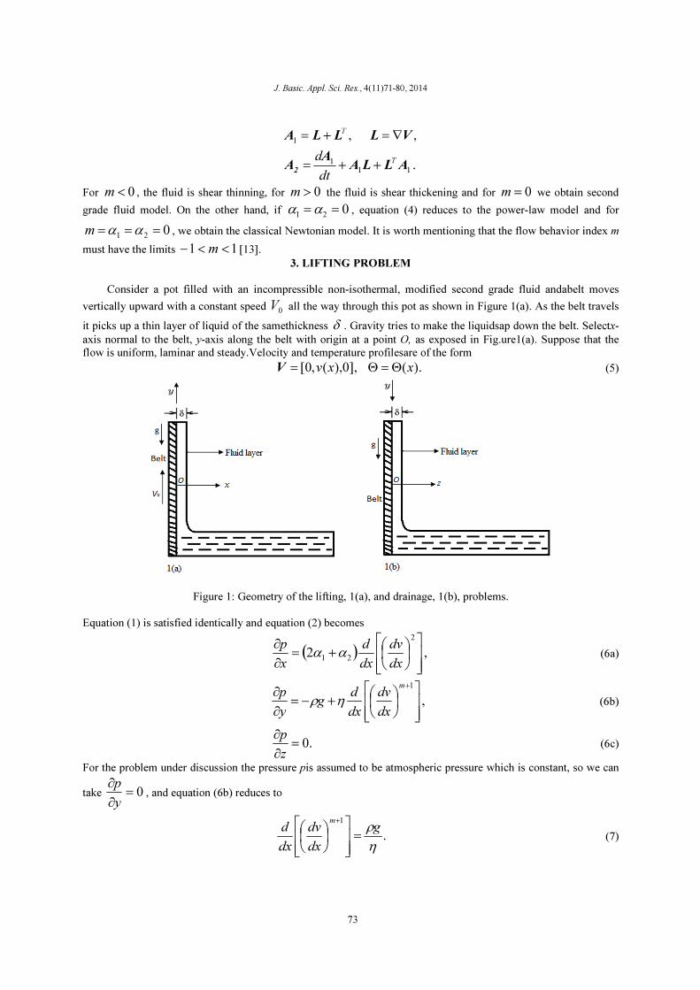
3. LIFTING PROBLEM
Consider a pot filled with an incompressible non-isothermal, modified second grade fluid andabelt moves
vertically upward with a constant speed 0
V all the way through this pot as shown in Figure 1(a). As the belt travels
it picks up a thin layer of liquid of the samethickness δ . Gravity tries to make the liquidsap down the belt. Selectx-
axis normal to the belt, y-axis along the belt with origin at a point O, as exposed in Fig.ure1(a). Suppose that the
flow is uniform, laminar and steady.Velocity and temperature profilesare of the form
).(],0),(,0[ xxv Θ=Θ=V (5)
Figure 1: Geometry of the lifting, 1(a), and drainage, 1(b), problems.
Equation (1) is satisfied identically and equation (2) becomes
( ) ,2
2
21
+=
∂
∂
dx
dv
dx
d
x
pαα (6a)
,
1
+−=
∂
∂+m
dx
dv
dx
dg
y
pηρ (6b)
.0=∂
∂
z
p (6c)
For the problem under discussion the pressure pis assumed to be atmospheric pressure which is constant, so we can
take 0=∂
∂
y
p, and equation (6b) reduces to
.
1
η
ρg
dx
dv
dx
dm
=
+
(7)
73
Farooq et al.,2014
By means of(5) the energy equation (3) we get
.
2
2
2 +
−=
Θm
dx
dv
dx
d
κ
η (8)
The associated boundary conditions for equations (7) and (8) are
.0,0
,0,00
δ==Θ
=
=Θ=Θ=
xatdx
d
dx
dv
xatVv
(9)
Integrating equation (7) with respect to x and usingthe appropriate boundary condition (9) we find that
( ) .1
11
1
+
+
−
−= m
m
xg
dx
dvδ
η
ρ (10)
Since velocity decreases with the increase of x so the sign of dx
dv is always opposite to that of x as can be seen in
equation (10). Now solving equations (10) together with (8) andapplingthe boundary conditions (9) we obtain
( ) ,2
1)( 1
2
1
21
1
0
−−
+
+
−= +
+
+
++
m
m
m
mm
xm
mgVxv δδ
η
ρ (11)
( )
( )( )( )
22
3 4 3 41
1 10
1( ) .
2 3 3 4
m
mmm
mm
m gx x
m m
η ρδ δ
κ η
+
+++
++
+ Θ = Θ + − −
+ + (12)
In solution (12), the second term inside the square brackets confirmdecline in temperature during the motion for any
x by keeping κη , etc. fixed. This is true for the velocity profile (11) also.Velocity profile for Newtonian
fluids(Munson5) is achieved by taking m=0, that is
,2
1)(
2
0
−−= xx
gVxv δ
η
ρ (11a)
where == effµη constant, kinematic viscosity for Newtonian fluid, and temperature for Newtonian fluid is
( )[ ].12
)(44
2
0x
gx −−
+Θ=Θ δδ
η
ρ
κ
η (12a)
4. VOLUME FLOW RATE, AVERAGE VELOCITY AND SHEAR STRESS FOR LIFTING PROBLEM
Volume flux is defined as
( ) ,
0
∫=δ
dxxvQ (13)
using velocity profile (11) becomes
.32
11
321
1
0
+
++
+
+−= m
mmg
m
mVQ δ
η
ρδ (14)
Average velocity, v , is given by
.
δ
Qv = (15)
Thus, average film velocity for the vertically upward moving belt is
74

J. Basic. Appl. Sci. Res., 4(11)71-80, 2014
.32
11
21
1
0
+
++
+
+−= m
mmg
m
mVv δ
η
ρ (16)
If we take 0>v in equation (16) the net upward flow of fluid can be obtained, i.e.,
,32
11
21
1
0
+
++
+
+> m
mmg
m
mV δ
η
ρ
whichgives a sensible estimate for the belt velocity to withdraw a modified second grade fluid.
Shear stress on the surface of the belt is
.
0
1
0
δρη gdx
dvT
x
m
xxy
−=
=
=
+
=
(17)
Introducing the following non-dimensional values
( )
22
0 0
0
1 0 1 0
* , * , * , * , , ,eff
t r
eff
UVv x gv x V S B
U U U
µρ δ
δ µ κ
Θ−Θ= = = Θ = = =
Θ −Θ Θ −Θ (18)
wheretS is Stokes number,
rB isBrinkman number,Uis characteristic velocity and
1Θ is characteristic temperature.
Using these dimensionless parameters, equations (11) and (12), after dropping the asterisk, become
( ) ( ) ,112
11
2
1
1
0
−−
+
+−= +
+
+ m
m
mt
xm
mSVxv (19)
( )( )
( )( )( ) ,11
4332
11
432
1
2
−−
++
+=Θ +
+
+
+
m
m
m
m
trx
mm
mSBx (20)
These are the non-dimensional velocity profile (equation (19)) and temperature distribution (equation (20))for
modified second grade fluid, respectively.
5. DRAINAGE PROBLEM
Now consider modified second grade fluid, falling on infinite vertical belt which is at rest as shown Figure
1(b). Here we choose y-axis along the belt in downward direction, z-axis perpendicular to the belt with origin at a
point O, as shown in Figure 1(b). The flow is in the downward direction due to gravity. Governing equations (2) and
(3) become
,
1
η
ρg
dz
dv
dz
dm
−=
+
(21)
,
2
2
2 +
−=
Θm
dz
dv
dz
d
κ
η (22)
along with the boundary conditions
.0,0
,0,00
δ==Θ
=
=Θ=Θ=
zatdz
d
dz
dv
zatv
(23)
Solving equations (21) and (22) with boundary conditions (23) we obtain
( ) ,2
1)( 1
2
1
21
1
−−
+
+
= +
+
+
++
m
m
m
mm
zm
mgzv δδ
η
ρ (24)
75

Farooq et al.,2014
( )
( )( )( )
22
3 4 3 41
1 10
1( ) .
2 3 3 4
m
mmm
mm
m gz z
m m
η ρδ δ
κ η
+
+++
++
+ Θ = Θ + − −
+ + (25)
For m=0, we obtain velocity profile for fluid as
,2
1)( 2
−= zz
gzv δ
η
ρ (24a)
and temperature profile becomes
( )[ ].12
)(44
2
0z
gz −−
+Θ=Θ δδ
η
ρ
κ
η (25a)
for Newtonian case.
6. VOLUME FLUX, AVERAGE FILM VELOCITY AND BELT SHEAR STRESS FOR DRAINAGE
PROBLEM
To calculate volume flux, Q , we use equation (24) in equation (13) to get
.32
11
321
1
+
++
+
+= m
mmg
m
mQ δ
η
ρ (26)
The average film velocity, v , is calculated as
.32
11
21
1
+
++
+
+= m
mmg
m
mv δ
η
ρ (27)
Shear stress on the belt becomes
.
0
1
0
δρη gdz
dvT
z
m
zyz
=
=
=
+
=
(28)
With the help of dimensionless parameters (18) equations (24) and (25) in the non-dimensional forms, after
dropping the ‘*’, become
( ) ( ) ,112
11
2
1
1
−−
+
+= +
+
+ m
m
mt
zSm
mzv (29)
( )( )
( )( )( ) ,11
4332
11
432
1
2
−−
++
+=Θ +
+
+
+
m
m
m
m
trz
mm
mSBz (30)
which are the velocity profile and temperature distribution for drainage problem, in the non-dimensional forms,
respectively.
7. RESULTS AND DISCUSSION
In the above sections we studied the thin film flows for lifting and drainage problems using a non-isothermal,
incompressible modified second grade fluid. We developed differential equations. The exact solutions for both cases
are obtained. We found that these solutions are dependent on the flow behavior index m, Stokes number t
S and
Brinkman numberr
B .The effect of flow behavior index mon the velocity field and temperature distribution for
shear thickening fluids is illustrated graphically through figures 2-3 and 6-7. For shear thinning fluids figures 5 and
9 are presented. Graphs for the Newtonian fluids are shown in figures 4 and 8. If the belt is moving vertically
upward, the magnitude of both velocity and temperature decrease as the fluid is becoming thicker and vice versa,
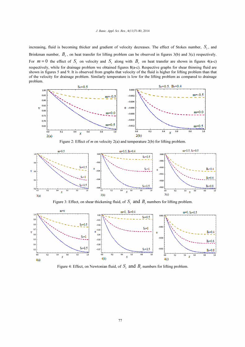
this can be observed in figures 2(a) and 2(b), while figures 6(a) and 6(b) are showing results for the drainage case.
Figure 3(a) is showing the effect of Stokes number, t
S , on velocity profile for lifting problem. We see that as t
S is
76
J. Basic. Appl. Sci. Res., 4(11)71-80, 2014
increasing, fluid is becoming thicker and gradient of velocity decreases. The effect of Stokes number, t
S , and
Brinkman number, r
B , on heat transfer for lifting problem can be observed in figures 3(b) and 3(c) respectively.
For 0=m the effect of t
S on velocity and t
S along with r
B on heat transfer are shown in figures 4(a-c)
respectively, while for drainage problem we obtained figures 8(a-c). Respective graphs for shear thinning fluid are
shown in figures 5 and 9. It is observed from graphs that velocity of the fluid is higher for lifting problem than that
of the velocity for drainage problem. Similarly temperature is low for the lifting problem as compared to drainage
problem.
Figure 2: Effect of m on velocity 2(a) and temperature 2(b) for lifting problem.
Figure 3: Effect, on shear thickening fluid, of rt
BS and numbers for lifting problem.
Figure 4: Effect, on Newtonian fluid, of rt
BS and numbers for lifting problem.
77

Farooq et al.,2014
Figure 5: Effect, on shear thinning fluid, of rt
BS and numbers for lifting problem.
Figure 6: Effect of m on velocity 6(a) and temperature 6(b) for drainage problem.
Figure 7: Effect, on shear thickening fluid, of rt
BS and numbers for drainage problem.
Figure 8: Effect, on Newtonian fluid, of rt
BS and numbers for drainage problem.
78

J. Basic. Appl. Sci. Res., 4(11)71-80, 2014
Figure 9: Effect, on shear thinning fluid, of rt
BS and numbers for drainage problem.
8. CONCLUSIONS
We have considered equations for steady, non-isothermal thin film flow for lifting and drainage problems of
modified second grade fluid and obtained exact solutions for both cases. We note that for m=0, solutions (11), (12)
for lifting problem and (24), (25) for drainage problem of the modified second grade fluid reduce to Newtonian
solutions (11a), (12a) and (24a), (25a) of respective problems. It is worthwhile to mention here that normal stresses
do not contribute for steady modified second grade fluid flow. Solutions (11) and (24) for velocity profiles and also
solutions (12) and (25) for temperature profiles are same as that of power law fluid, we do not see any contribution
of the modified second grade fluid model verses power law model. There will be a net upward flow if 0>v , that
is, non-dimensional 0
V must be greater than .32
11
1
+
+
+m
tS
m
m For Newtonian fluid
0V must be greater than .
3
1
tS
For fixed value of the Stokes number, t
S , the inverse relation has been observed between the flow behavior index m
and the nature of the velocity, as illustrated in figures 2(a) and 6(b) respectively.
REFERENCES
1. T.C. Papanastasiou, 1994. Applied Fluid Mechanics, P T R Prentice Hall.
2. K. Sadeghy, A.H. Najafi, M. Saffaripour, 2005. Int. J. Non-Linear Mech., 40: 1220-1228.
3. J.E. Dunn, K.R. Rajagopal, 1995. Fluids of differential type: critical review and thermodynamic analysis.
Int. J. Engg. Sci., 33(5): 689-729.
4. R.P. Chhabra, J.F. Richardson, 1999. Non-Newtonian Flow in the Process Industries: Fundamentals and
Engineering Applications, Butterworth-Heinemann, London.
5. B.R. Munson, 2006. Fundamentals of fluid mechanics. John Wiley and Sons, Inc.
6. A.M. Siddiqui, R. Mahmood, Q.K. Ghori, 2006. Some exact solutions for the thin film flow of a PTT fluid.
Phys. Lett. A, 356: 353–356.
7. A.M. Siddiqui, R.Mahmood, Q.K. Ghori, 2006. Homotopy perturbation method for thin film flow of a
fourth grade fluid down a vertical cylinder. Phys. Lett. A, 352: 404-410.
8. A.M. Siddiqui, M. Ahmed, Q.K. Ghori, 2007.Thin film flow of non-Newtonian fluids on a moving belt.
Chaos Solitons Fractals, 33: 1006-1016.
9. A.M. Siddiqui, R. Mahmood, Q.K. Ghori, 2008. Homotopy perturbation method for thin film flow of a
third grade fluid down an inclined plane. Chaos Solitons Fractals, 35: 140-147.
10. H.I. Andersson, D.Y. Shang, 1998. An extended study of the hydrodynamics of gravity-driven film flow of
power-law fluids. Fluid Dyn. Res., 22: 345-357.
11. B.K. Rao, 1999. Heat transfer to a falling power-law fluid film. Int. J. Heat Fluid Flow, 20: 429-436.
79

Farooq et al.,2014
12. D.Y. Shang, H.I. Andersson, 1999. Heat transfer in gravity-driven film flow of power-law fluids, Int. J.
Heat Mass Transfer, 42: 2085-2099.
13. C. Wang, I. Pop, Analysis of the flow of a power-law fluid film on an unsteady stretching surface by means
of homotopy analysis method. J. Non-Newtonian Fluid Mech., 138: 161–172.
14. M. K. Alam, A. M. Siddiqui, M. T. Rahim, S. Islam, 2012. Thin-film flow of magnetohydrodynamic
(MHD) Johnson-Segalman fluid on vertical surfaces using the Adomian decomposition method, Appl.
Math. Comput., 219 (8): 3956-3974.
15. M.K. Alam, M.T. Rahim, E.J. Avital, S. Islam, A.M. Siddiqui, J.J.R. Williams, 2013. Solution of the steady
thin film flow of non-Newtonian fluid on vertical cylinder using Adomian Decomposition Method, Journal
of the Franklin Institute, 350(4):818–839.
16. F. Ahmad, S. Hussain, 2014. Heat transfer and MHD boundary layer flow over a rotating disk, J. Basic.
Appl. Sci. Res., 4(1): 327-331.
17. S. Hussain, F. Ahmad, 2014. MHD Flow of Micropolar Fluids over a Shrinking Sheet with Mass Suction,
J. Basic. Appl. Sci. Res., 4(2): 174-179.
18. C.Y. Wang, 1991. Exact solutions of the steady-state Navier-Stockes equations, Annu. Rev. Fluid Mech.
23: 159-177.
19. C.Y. Wang, 1966. On a class of exact solutions of the Navier-Stokes equations, J. Appl. Mech. 33: 696-
698.
20. C.Y. Wang, 1989. Exact solutions of the unsteady Navier-Stokes equations. Appl. Mech. Rev., 42(a): 269-
282.
21. R. Ullah, G. Zaman, S. Islam, 2013. Stability analysis of a general SIR epidemic model, VFAST
Transactions on Mathematics, 1(1): 16-20.
22. S.F. Saddiq, M.A. Khan, S.A. Khan, F. Ahmad, M. Ullah 2013. Analytical solution of an SEIV epidemic
model by Homotopy Perturbation method, VFAST Transactions on Mathematics, 1(2): 1-7.
80