Ex-ante and Ex-post Effects of Price Limits in

Commodity Futures Markets

by

Gabriel Blair Fontinelle and Joseph P. Janzen

Suggested citation format:

Fontinelle, G. B. and J. P. Janzen. 2020. “Ex-ante and Ex-post Effects of Price

Limits in Commodity Futures Markets.” Proceedings of the NCCC-134

Conference on Applied Commodity Price Analysis, Forecasting, and Market Risk

Management. [http://www.farmdoc.illinois.edu/nccc134].

1

Ex-ante and ex-post effects of price limits in commodity futures markets

Gabriel Blair Fontinelle

Dept of Agricultural Economics, Kansas State University

342 Waters Hall, 1603 Old Claflin Pl, Manhattan, KS, 66506, USA

Email: gblair@ksu.edu

Joseph P. Janzen

Dept of Agricultural Economics, Kansas State University

337A Waters Hall, 1603 Old Claflin Pl, Manhattan, KS, 66506, USA

Email: jjanzen@ksu.edu

Paper prepared for the NCCC-134 Conference on Applied Commodity Price Analysis,

Forecasting, and Market Risk Management, 2020.

Copyright 2020 by Gabriel Blair Fontinelle and Joseph P. Janzen. All rights reserved. Readers

may make verbatim copies of this document for non-commercial purposes by any means,

provided that this copyright notice appears on all such copies.

2

Ex-ante and ex-post effects of price limits in commodity futures markets

After October 1987, financial crisis, market regulators created dispositive called circuit

breaks to contain high levels of volatility. As a type of circuit break, price limits were adopted

not only on stock markets but in commodity futures contracts as well, however, its effects are not

clear. The present study aimed to evaluate price limit ex-ante effects on the four major wheat

futures markets by adopting Brogaard and Roshak (2015) methodology by estimating the

probability of extreme movements and limit moves conditional to extreme movements and its ex-

post effects on trading activity by contrasting the volume curve on limit days with a

counterfactual volume curve that simulates a scenario where price limits were not hit. The

results show that tighter limit levels decrease the probability of extreme movements by

approximately 0.008% having an overall (four markets included) baseline probability of extreme

moves equals 1.11% which agrees with the Holding Back hypothesis assuming extreme

movements as a proxy for volatility. On the other hand, the probability of limit moves conditional

to extreme movements increases when limit levels are tighter by approximately 0.066% with an

overall baseline of 0.05% which supports the “Magnet” hypothesis. Regarding the ex-post

effects, longer periods where prices stay at the limit level result in trading activity lost, however,

if prices return to limit range but bounce back to a limit lock, the longer the gap between limit

locks trading session experience an increase in trading activity. Moreoever, the ex-post effects

on trading activity are more intense in Chicago relative to Kansas City because Chicago present

a higher trading volume on average.

Key words: circuit breaker, price limits, trading activity, ex-ante effect, ex-post effect

Introduction

Commodity futures markets are used by producers and consumers as a risk management tool to

hedge themselves against price risk. Therefore, futures prices need to be trustworthy benchmarks

of the actual value of the underlying commodity. To guarantee price integrity, futures market

prices should be subject to volatility derived from fundamental supply and demand factors but

not volatility coming from non-fundamental reasons. In particular, futures prices should not be

subject to bubbles and other feedback loops where high prices lead to even higher prices.

Exchanges use mechanisms called circuit breakers which aiming to halt trading when this latter

kind of volatility causes prices to overreact. Trading halts and price limits are examples of circuit

breaks used by exchanges around the globe and cast multiple viewpoints about its effectiveness.

Proponents would say that circuit breaks work as a speed bump in a rapid decline or increase.

Critics would say that circuit breaks that interruptions inhibit efficient pricing.

To illustrate how they work, trading halts were created after the October 1987 market crash and

are based on levels of change in price relative to the previous close. For instance, On S&P 500

index, NYSE sets three levels of change in price as their threshold, 7%, 13%, and 20%. If the

index has a change in the price of 7% up or down, there is a trading halt of 15 minutes. After this

period trade resumes and, if the second level gets hit, then another trading halt of 15 minutes is

triggered. In case the third level gets hit, then trading stops for the rest of the day.

For price limits, let’s consider that a certain exchange based on previous price behavior set a

price limit of 55 cents for the corn futures contract. If the previous settlement price was $3.75 per

bushel, the limit range would be between $ 4.30 and $3.20 per bushel. As a form of “too far, too

3

fast” condition to restrict volatility, price limits are set based on current market information

aiming to resemble a realistic volatility status. In more detail, the limit range is established daily

by a specific amount higher or lower than the previous day’s settlement price. Nonetheless,

restrict price to freely ranges brings questions regarding its effects on price behavior before and

after a limit move. Price limits are the most used method to mitigate price volatility in

commodity futures markets since the 20th century and is the focus of this study since its effects

on this markets are still unclear Daily price limits may affect trading activity and prices after

prices hit limit bounds (ex-post) and before a limit hit (ex-ante). In theory, price limits were

developed to restrain excessive volatility that could drive prices quickly to levels not sustained

by fundamental reasons, but skeptical to the policy would say the opposite due to its effect on

trading behavior. Moreover, with limits, there is no direct way to calculate the impairment

caused on trading activity since the alternative scenario where limits do not apply doesn’t apply

to the same market circumstances. With that, what are the ex-ante effects of price limits that

could influence prices to get to the limit? Moreover, what is the comportment of trading activity

before, when the limit gets hit and after?

Price limits ex-ante effects could be reflected in trade behavior. Traders could use limit levels as

a signal to develop their strategies. In face of a high volatility period and extreme move in price

leading it to the limit level, traders could anticipate their trades as they visualize a real chance

that price hits the limit which Subrahmanyam (1994) addresses as the “Magnet” hypothesis. The

opposite could also happen, where traders in face of a high volatility period would delay their

orders for a stillness moment when prices would be subjected to regular levels of volatility

described by Subrahmanyam (1997). A good way to untangle this dilemma is to estimate the

likelihood of extreme moves or limit hits conditional to price limits in the commodity futures

market.

Trading activity empirically is affected on both moments, before and after a limit hit essentially

being shifting back and forward, however, its main change is observed from an ex-post

perspective. Right before a limit hit, volume tends to spike to levels relatively similar to the open

or close decreasing drastically during the period where the limit is locked and resuming with

another peak if prices return to levels below the limit. This market phenomenon fairly looks like

another U-shaped pattern investigated by Admati and Pfleiderer (1988) inside the day. This shift

in trading activity would certainly impose a cost. Without a scenario where price limits are not

applied, one way to overcome this obstacle is to estimate this cost by calculating the difference

in trading activity between the volume in a limit day and a counterfactual scenario that would

represent the absence of price limits.

This paper assesses the effects of price limits on price behavior before and after limits are hit.

We also estimate the realized costs of imposing price limits in terms of shifted trading activity.

Both efforts rely on the presence of other unconstrained or less constrained markets to estimate

the relevant counterfactual and trading activity that would have occurred in the absence of price

limits. To better identify this counterfactual, we apply our analysis to the wheat futures complex,

the four actively traded and liquid wheat futures contracts originally based in Chicago, Kansas

City, Minneapolis, and Paris.

In the ex-ante sphere, we use a similar methodology as Brogaard and Roshak (2015) on

estimating the probability of a limit move and an extreme move conditional to specific features

of the commodity futures market through a Difference-in-difference linear probability model. In

our study, three elements are crucial to set our model. First is the possibility to test price limit

policy as our treatment by using the Paris wheat futures contract as our control which is feasible

4

by not being under the price limit regime. Second is based in the fact that after the commodity

boom in 2008, due to frequent large price changes, CME Group abandoned a constant price limit

and established a periodical review on limit levels for various commodities which is the

treatment in our model to answer if a tighter limit level increase or decrease the likelihood of a

limit move. Third is in our definition of extreme movements. Price changes equivalent to 25

cents are addressed as extreme movements. Knowing the likelihood of extreme movements can

enlighting the ex-ante effects of price limit on price behavior.

Trading activity could also be subjective to the ex-post effects of price limits. Admati and

Pfleiderer (1988) investigate intraday patterns in stocks evoking the U-shaped theory over

volume. We can apply this concept in commodity futures since empirically daily volume behaves

in a U-shaped curve (volume peak at the opening following by lower levels throughout the

trading session and surging again at the end of the trading session). Theoretically, if there is an

ex-post effect of price limits, a volume U-shaped pattern could be observed where volume peak

at the moment prices hit the limit level and reduces as prices keep locked at the limit level

following by a considerable increase when prices return to price range. Unfortunately, a little has

been discussed in the literature about trading activity and price limits in agricultural commodity

markets, therefore this is study throw light on the subject.

As our ex-ante effects estimates, a tighter limit level reduces the probability of an extreme

movement for both treated and control variables, which corroborate with the “Holding Back”

hypothesis taking extreme movements as a proxy for volatility as Brogaard and Roshak (2015).

However, regarding the probability of limit moves conditional to extreme movements, we

observe the opposite conclusion. A tighter limit level increases the likelihood of a limit move

corroborating with the “Magnet” hypothesis suggested by (Subrahmanyam, 1994). Ex-post

effects of price limit on trading activity have a similar ambiguous behavior. Trading activity has

a unique behavior when prices are about to hit the limit. Around a limit hit, trading activity shifts

concentrating seconds before a limit hit and creating a peak on volume. Seconds before the hit,

trading activity tends to reduce drastically surging again if prices return inside the limit bound.

This behavior is subject most by how long prices will stay at the limit level and/or if prices will

hit the limit level multiple times in a session. Our results indicate that the longer is the period

where prices are at the limit, the greater is the trading activity loss in comparison with a possible

scenario where price limits would not apply which is expressed by our counterfactual volume

curve. Moreover, if prices hit the limit level multiple times in a session and the time between hits

are longer, the trading session can experience an increase in trading activity since volume speak

right before the limit hit is not compensated by the loss in trading activity when price stay at the

limit for a longer time.

1

Methodology

For this study, we use daily and intraday wheat futures contracts price and volume data from

January 2007 to April 2019 for the world wheat futures market complex: the Chicago Mercantile

Exchange (CME) Soft Red Winter Wheat (SRW) and Kansas City Hard Red Winter Wheat (KC

HRW) contracts, the Minneapolis Grain Exchange (MGEX) Hard Red Spring Wheat (HRSW)

contract, and Euronext Milling Wheat N° 2 (EBM) contract. For brevity, we refer to each

contract using the city with which it is commonly associated (i.e. Chicago, Kansas City,

Minneapolis, and Paris, respectively). For Paris data, prices are converted to US currency and

quantity aiming to match CME price and contract specification.

Daily price data were collected from Bloomberg Terminal. For each year, all delivery months are

collected it, however after 2015, Euronext changes its delivery months for wheat contracts. For

Euronext EBM contracts, the delivery months are November (X), January (F), March (H) and

May (K) until May 2015 and then September (U), December (Z), March (H) and May (K) from

September 2015 onwards. In respect to CME contracts, SRW and KC HRW cover March (H),

May (K), July (N), September (U) and December (Z).

Intraday price and volume data were purchased from CQG Inc. Data is available for the Kansas

City, Chicago, and Paris contracts. This data reports the price and volume for every trade in each

market in chronological order, time-stamped to the minute.

There are two sections in our methodology. The first one describes all procedures and models to

estimate the ex-ante effects of price limits by estimating the probabilities of extreme movements

and limit movements under different conditions. The second describes all procedures to estimate

ex-post effects of price limit on volume by constructing a counterfactual volume curve to project

what would happen with trade activity if there were no limit hits. With that, we compare our

counterfactual volume with the actual volume during limit days to assess price limits effect on

trading activity and estimate its costs.

Price limit ex-ante evaluation

To evaluate ex-ante effects of price limits, market moments and factors have to be taken into

consideration whereas they could influence price trajectory towards the limit. Our selected

market moment is the existence of extreme movements. Large price move could be associated

with limit hits as traders could use those as a signal to anticipate or delay their orders. Moreover,

price limit levels and even other market factors like volatility, more active market, and public

report releases could affect the likelihood of an extreme movement or even a limit hit. Therefore,

to assess the ex-ante effects of price limits we estimate the probability of extreme movements

and the probability of limit moves conditional to extreme movements in the wheat futures market

complex, in a difference-in-difference approach using Linear Probability Model (LPM) adapted

from Brogaard & Roshak (2015). With that we estimate:

• P(extreme movements)

The Probability of extreme movements due to different markets, limit levels, limit level changes

through time, volume, days to expiration, delivery period, and exogenous variables such as VIX

Index, and fundamental reports (i.e. WASDE).

2

• P(Limit movements | extreme movements)

Probability of limit movements given extreme movements happened due to different markets,

limit level, limit level changes through time, volume, days to expiration, and exogenous

variables such as VIX Index, and fundamental reports (i.e. WASDE).

The Difference-in-difference approach is possible since Paris contracts do not use daily price

limit policy. Moreover, CME Group resets the daily price limit every six months since 2014

which gives variation in the “treatment” variable across time. The analysis imposes extreme

movements as an oscillation in price greater or equal to 25 cents. For limit move, change in price

relative to the previous day price close must be biding with the respective daily limit on the

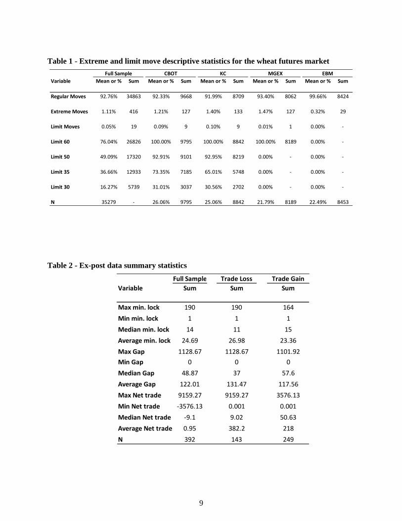
given day. CME group reset the daily price limit levels every six months since 2014. Figure 1

shows how daily price limit levels behave through time. Before 2014, limit levels were constant

and just had a reset process in 2008 due to the commodity boom prices which made limit moves

more frequent since limit levels were not effective to those volatility levels. The first reset

happens in May based on the average of the settlement price from the 45 consecutive days of the

nearest July contract before and on the business day before April 16th. The calculated average

multiplied by 7% and rounded to the nearest 5 cents per bushel, or 30 cents per contract,

whichever is higher, will be the preliminary initial price limit. The same procedure is done to KC

HRW contract and the higher preliminary initial price limit will be the new initial price limit for

Wheat futures and will become effective on the first trading day in May until the last trading day

in October.

The second reset occurs on the first trading day in November based on the average of the

settlement price from the 45 consecutive days of the nearest December contract before and on

the business day before October 16th. The calculated average multiplied by 7% and rounded to

the nearest 5 cents per bushel, or 30 cents per contract, whichever is higher, will be the

preliminary initial price limit. The same procedure is applied to the Kansas City contract and the

higher preliminary initial price limit will be the new initial price limit for Wheat futures and will

become effective on the first trading day in November until the last trading day in next April.

Those changes in price limit levels are important to our model to evaluate the effect of price

level changes through time on estimate probabilities. Minneapolis's daily limit is fixed in 30

cents for the whole period.

Extreme move probability models

Our study proposes two models for each extreme move probability estimative. The first model

estimating the probability of extreme movements discriminating price limit in levels. The second

model discriminate price limit levels as “tight” or not relative to the previous price limit level.

Our first model for P(Extreme movements) is shown in Equation 1.

(1) 𝐸𝑥𝑡𝑟𝑒𝑚𝑒𝑚,𝑐,𝑡 = 𝛽0 + ∑ 𝛽

4

𝑚=1

𝑀𝑎𝑟𝑘𝑒𝑡𝑠𝑚,𝑡 + 𝛽5𝐿𝑖𝑚𝑖𝑡50𝑚,𝑐,𝑡 + 𝛽6𝐿𝑖𝑚𝑖𝑡35𝑚,𝑐,𝑡 + 𝛽7𝐿𝑖𝑚𝑖𝑡30𝑚,𝑐,𝑡 + ∑ 𝛽

10

𝑛=1

𝑅𝑒𝑠𝑒𝑡𝑚,𝑐,𝑡

+ 𝛽18𝐿𝑎𝑔𝐸𝑥𝑡𝑟𝑒𝑚𝑒𝑚,𝑐,𝑡 + 𝛽19𝐿𝑎𝑔𝐿𝑖𝑚𝑖𝑡𝑀𝑜𝑣𝑒𝑚,𝑐,𝑡 + 𝛽20𝐿𝑖𝑓𝑒𝑚,𝑐,𝑡 + 𝛽21𝐷𝑒𝑙𝑖𝑣𝑒𝑟𝑦𝑚,𝑐,𝑡 + 𝛽22𝑉𝐼𝑋𝑡

+ 𝛽23𝑅𝐸𝑃𝑂𝑅𝑇𝑆𝑡

Extreme is a dummy variable equal to 1 if, on market m, contract c at day t experienced an

extreme movement. Markets are dummy variables to discriminate which of the four markets the

contract c belongs (i.e CBOT, KC, MGEX or Euronext-Paris) at day t. Limit50, Limit35, and

Limit30 are dummy variables to express the price limit levels on market m, contract c at day t.

Limit50 is equal to unity for price limit levels less or equal to 50 cents and 0 otherwise. Limit35

3

is equal to unity for price limit levels less or equal to 35 and 0 otherwise and Limit30 is equal to

unity for price limit levels less or equal to 30 and 0 otherwise. The ten Reset variables are

dummy variables for each reset on price limit levels in CBOT and KC which happens every 6

months. Lag Extreme for market m, contract c, and day t is a dummy variable equal to one if the

previous day experienced a extreme movement. Lag Limit Move for market m, contract c, and

day t is a dummy variable equal to one if the previous day experienced a limit move. Life

variable corresponds to days before the expiration on market m, for contract c at day t. Delivery

is a dummy variable standing for the delivery period (last twelve days of the contract) when price

limits are not applied and are equal to 1 when contracts are at this period or 0 otherwise. The

exogenous variables are VIX for CBOE Volatility index and REPORTS is expressed as a dummy

variable equals to 1 for time t when a fundamental report is released (i.e. WASDE).

(2) 𝐸𝑥𝑡𝑟𝑒𝑚𝑒𝑚,𝑐,𝑡 = 𝛽0 + ∑ 𝛽

4

𝑚=1

𝑀𝑎𝑟𝑘𝑒𝑡𝑠𝑚,𝑡 + 𝛽5𝑇𝑖𝑔ℎ𝑡𝑚,𝑐,𝑡 + ∑ 𝛽

10

𝑛=1

𝑅𝑒𝑠𝑒𝑡𝑚,𝑐,𝑡 + 𝛽16𝐿𝑎𝑔𝐸𝑥𝑡𝑟𝑒𝑚𝑒𝑚,𝑐,𝑡

+ 𝛽17𝐿𝑎𝑔𝐿𝑖𝑚𝑖𝑡𝑀𝑜𝑣𝑒𝑚,𝑐,𝑡 + 𝛽18𝐿𝑖𝑓𝑒𝑚,𝑐,𝑡 + 𝛽19𝐷𝑒𝑙𝑖𝑣𝑒𝑟𝑦𝑚,𝑐,𝑡 + 𝛽20𝑉𝐼𝑋𝑡 + 𝛽21𝑅𝐸𝑃𝑂𝑅𝑇𝑆𝑡

The second model for P(Extreme movements) is shown in equation 2. All variables are the same

except that Limit50, Limit35, and Limit30 are replaced by Tight which is a dummy variable

equals to unity when the daily limit is narrower relative to the previous level and 0 otherwise.

The Tight variable is an attempt to synthesize the dynamic effect of limit levels due to its

periodical reset. In theory, tighter limits could increase the probability of extreme movements

and limit move since the price range allowed is narrow in comparison with the previous price

range established by the limit bounds.

Limit move probability models

We design two models to estimate the probability of limit moves. The third model uses the same

concept as those models before, however, it estimates a conditional probability of a limit

movement given an extreme movement occurrence and is shown in Equation 3:

(3) 𝐿𝑖𝑚𝑖𝑡𝑀𝑜𝑣𝑒𝑚,𝑐,𝑡 = 𝛽0 + ∑ 𝛽

4

𝑚=1

𝑀𝑎𝑟𝑘𝑒𝑡𝑠𝑚,𝑡 + 𝛽5𝐿𝑖𝑚𝑖𝑡50𝑚,𝑐,𝑡 + 𝛽6𝐿𝑖𝑚𝑖𝑡35𝑚,𝑐,𝑡 + 𝛽7𝐿𝑖𝑚𝑖𝑡30𝑚,𝑐,𝑡 + ∑ 𝛽

10

𝑛=1

𝑅𝑒𝑠𝑒𝑡𝑚,𝑐,𝑡

+ 𝛽18𝐿𝑎𝑔𝐸𝑥𝑡𝑟𝑒𝑚𝑒𝑚,𝑐,𝑡 + 𝛽19𝐿𝑎𝑔𝐿𝑖𝑚𝑖𝑡𝑀𝑜𝑣𝑒𝑚,𝑐,𝑡 + 𝛽20𝐿𝑖𝑓𝑒𝑚,𝑐,𝑡 + 𝛽21𝑉𝐼𝑋𝑡 + 𝛽22𝑅𝐸𝑃𝑂𝑅𝑇𝑆𝑡

LimitMove is a dummy variable equals to unity when the difference in price relative to previous

day close price on market m, contract c, at day t is binding with the limit level at day t or 0

otherwise. All other variables are the same as Equation 1 except for Delivery which during that

period price limits do not apply.

As our fourth model, a conditional probability of a limit movement given an extreme movement

occurrence is shown in Equation 4. The variables are the same as Equation 3, however, limit

levels are replaced by Tight variable, which is a dummy variable equal to unity when the limit

price level is tighter or equal relative to the previous price limit level.

(4) 𝐿𝑖𝑚𝑖𝑡𝑀𝑜𝑣𝑒𝑚,𝑐,𝑡 = 𝛽0 + ∑ 𝛽

4

𝑚=1

𝑀𝑎𝑟𝑘𝑒𝑡𝑠𝑚,𝑡 + 𝛽5𝑇𝑖𝑔ℎ𝑡𝑚,𝑐,𝑡 + ∑ 𝛽

10

𝑛=1

𝑅𝑒𝑠𝑒𝑡𝑚,𝑐,𝑡 + 𝛽16𝐿𝑎𝑔𝐸𝑥𝑡𝑟𝑒𝑚𝑒𝑚,𝑐,𝑡 + 𝛽17𝐿𝑎𝑔𝐿𝑖𝑚𝑖𝑡𝑀𝑜𝑣𝑒𝑚,𝑐,𝑡

+ 𝛽18𝐿𝑖𝑓𝑒𝑚,𝑐,𝑡 + 𝛽19𝑉𝐼𝑋𝑡 + 𝛽20𝑅𝐸𝑃𝑂𝑅𝑇𝑆𝑡

After evaluating the probabilities estimated for each model, the models with greater performance

are used to display estimate probabilities using our control (Paris) data and other three markets

4

(CBOT, KC, and MGEX) aiming to evaluate our treatments (reset window period) in a

difference-in-difference layout. The plots are confronted with the regression coefficients for each

probability estimate.

Price limit ex-post evaluation

To estimate the ex-post effects of price limits we assess how limit moves affect trading activity

using intraday data of wheat futures contract from two major markets, Chicago and Kansas City.

Our data are composed of 392 limit days occurred in Chicago and Kansas City from 2008 until

2017.The data shows that trading activity can be shifted according to limit hit and its duration.

The longer price limits bind the more likely it becomes that trading volume is curtailed. In

contrast, a short period with limit bonded, could likely behave as a price shock and increase

trading activity. Additionally, volume peak could happen moments before the limit hit, thus

indicating a lag effect of price limits on trading activity. Changes in trading activity could result

in costs such as a decrease in price discovery and trading activity lost. Consequently, we estimate

the ex-post effect of price limits on trading activity by observing the behavior of volume during a

limit move day and compare it with a counterfactual volume curve which is a representation of

what could happen with volume if there was no limit hit.

The intraday data used has a minute resolution allowing to identify the exact minute when prices

hit the limit, however not exactly when inside the minute. Since electronic trading enables a

larger number of orders to be executed in seconds, this resolution prevents us to measure how

much trading activity we have before, before, at the limit, and during the limit lock. To overcome

this limitation, since the filled orders are placed chronologically in the data, we manage it to

equally distribute all trades that happened within a minute yielding a “sequential intra-minute”

time-bin resolution. After arranging the data to this resolution, we construct our counterfactual

volume curve. We measure the net loss or gain of trading activity due to limit hits as the

difference between actual volume on the limit day and counterfactual volume before, during, and

after the period where a lock-limit event occurs. The counterfactual volume series estimates what

would have happened if trading was not halted due to the limit. To preserve any market

condition in favor of a realistic comparison we estimate counterfactual volume using the average

intraday volume in each time-bin using the average over the last 5-7 days. To accommodate

higher average trading volume in general on limit move days we adjust our counterfactual

volume series to narrow any possible gap between volume levels since days that are not limit

move days and are used to compute our counterfactual tend to present lower daily volume on

average.

(5) 𝐴𝑑𝑗𝑢𝑠𝑡𝑒𝑑 𝐶𝑜𝑢𝑛𝑡𝑒𝑟𝑓𝑎𝑐𝑡𝑢𝑎𝑙 𝑉𝑜𝑙𝑢𝑚𝑒𝑚,𝑐,𝑡,𝑖 = 𝐶𝑜𝑢𝑛𝑡𝑒𝑟𝑓𝑎𝑐𝑡𝑢𝑎𝑙 𝑉𝑜𝑙𝑢𝑚𝑒𝑚,𝑐,𝑡,𝑖 ∑ 𝐴𝑐𝑡𝑢𝑎𝑙 𝑉𝑜𝑙𝑢𝑚𝑒 𝑙𝑖𝑚𝑖𝑡 𝑑𝑎𝑦𝑚,𝑐,𝑡,𝑖

𝑛𝑖=1

∑ 𝐶𝑜𝑢𝑛𝑡𝑒𝑟𝑓𝑎𝑐𝑡𝑢𝑎𝑙 𝑣𝑜𝑙𝑢𝑚𝑒𝑚,𝑐,𝑡,𝑖𝑛𝑖=1

Where the Adjusted Counterfactual Volume on market m, contract c, day t at time bin i is equal

to the Counterfactual Volume for market m, contract c, day t at time bin i multiplied by the ratio

between the total Actual Volume and the total Counterfactual Volume on market m, contract c,

day t at time bin i. With the counterfactual adjusted, the data is merged based on the time-bin

stamp and the Net Trade variable on market m, contract c at limit day t is calculated which is

essentially the difference between the total Adjusted Counterfactual Volume on limit day t for all

time-bin i and the total Actual Volume on limit day t for all time-bin i.

5

(6) 𝑁𝑒𝑡 𝑇𝑟𝑎𝑑𝑒𝑚,𝑐,𝑡 = ∑ 𝐴𝑑𝑗𝑢𝑠𝑡𝑒𝑑 𝐶𝑜𝑢𝑛𝑡𝑒𝑟𝑓𝑎𝑐𝑡𝑢𝑎𝑙 𝑉𝑜𝑙𝑢𝑚𝑒𝑚,𝑐,𝑡,𝑖

𝑛

𝑖=1

− ∑ 𝐴𝑐𝑡𝑢𝑎𝑙 𝑉𝑜𝑙𝑢𝑚𝑒 𝑙𝑖𝑚𝑖𝑡 𝑑𝑎𝑦𝑚,𝑐,𝑡,𝑖

𝑛

𝑖=1

Trading volume generally is larger than the counterfactual right before and at the period when

the limit hits and lower when the limit has been hit for a long time. When prices return to levels

inside the limit bound, trading volume peaks again creating a similar U-shaped pattern. This

illustrates that price limits have a lag effect on trading activity. Therefore, three variables are

created to capture those effects. The Min. Lock variable, which is the sum of minutes when

prices stayed locked on the limit level on market m, contract c at limit day t is created to capture

the duration effect. Since prices are locked at the limit level, some market participants

understand that prices are not realistic and reduce their trades at this level thus reducing trading

activity. The Min. lock with Gap variable is the period starting from the moment of the first limit

hit until the end of the last limit hit on market m, contract c at limit day t and is calculated to

make able to get our third variable The Gap variable is essentially the total minutes that prices

are not locked at the limit level between the moment of the first limit hit until the end of the last

limit hit and controls the lag effect of price limits on trading activity.

(7) 𝐺𝑎𝑝𝑚,𝑐,𝑡 = 𝑀𝑖𝑛. 𝐿𝑜𝑐𝑘𝑚,𝑐,𝑡 − 𝑀𝑖𝑛. 𝐿𝑜𝑐𝑘𝑊𝑖𝑡ℎ𝐺𝑎𝑝𝑚,𝑐,𝑡

Trading activity dynamic models

Positive values of net trade indicate trading activity loss because the counterfactual volume is

higher than the actual volume. Due to the limit hit, part of the volume who was supposed to exist

based on our counterfactual volume curve is lost. On the other hand, negative values of net trade

indicate trading activity gain. The actual volume during a limit day is greater than our

counterfactual volume curve which shows an increment on trade activity due to the limit hit.

To identify relationships between our measure of the trading volume change in trading volume

caused by the imposition of price limits, we estimate five regression models with net trade as the

dependent variable. The first model considers the level of Net Trade as a function of Min Lock,

Gap, Total Volume and our control variables Lag Extreme, Vix, Report, and Life used on

previous models for our ex-ante analysis. The second model estimates exclusively the level trade

loss (positive net trade values) using the same controls as the first model control variables and

the third one estimates exclusively the level of trade gains (negative net trade values) using the

control variables used before. Our fourth and fifth model is similar to second and third, however,

our dependent variables are expressed in natural logarithm form to provide margin effects in

percentage (Log-level coefficients)

For the first model, we use Net trade on market m, contract c at limit day t as our dependent

variable without distinguishing positive and negative values. As our control variables, KC is a

dummy variable equals unity when Net trade happens on Kansas City wheat contract c at limit

day t. Min.Lock is the sum of minutes that price stayed locked on the limit level on market m,

contract c at limit day t. The Gap is the total amount of minutes where the price is not locked at

the limit level between the moment of the first limit hit until the end of the last limit hit on

market m, contract c at limit day t. The variables KC_Min.lock and KC_Gap are interaction

variables between our Market variable KC and our variables of interest Min.lock and Gap. They

are created in order to know the intensity of the effect of our variables of interest on trading

activity for both markets, Kansas City and Chigaco. TotalVol is the total volume on market m,

contract c at limit day t. LagExtreme is a dummy variable equals to unity when the day before a

limit day t, on market m and contract c (price change equals or greater than 25 cents). VIX

6

represents the CBOE Volatility index at limit day t. Report is a dummy variable equals unity

when any supply and demand related report is release at limit day t and Life is the number of

days before the expiration of contract c, on market m at limit day t.

(7) 𝑁𝑒𝑡 𝑡𝑟𝑎𝑑𝑒𝑚,𝑐,𝑡 = 𝛽0 + 𝛽1𝐾𝐶𝑡 + 𝛽2𝑀𝑖𝑛. 𝐿𝑜𝑐𝑘𝑚,𝑐,𝑡 + 𝛽3𝐾𝐶_𝑀𝑖𝑛. 𝑙𝑜𝑐𝑘𝑚,𝑐,𝑡 + 𝛽4𝐺𝑎𝑝𝑚,𝑐,𝑡 + 𝛽5𝐾𝐶_𝐺𝑎𝑝𝑚,𝑐,𝑡

+ 𝛽6𝑇𝑜𝑡𝑎𝑙𝑉𝑜𝑙𝑚,𝑐,𝑡 + 𝛽7𝐿𝑎𝑔𝐸𝑥𝑡𝑟𝑒𝑚𝑒𝑚,𝑐,𝑡 + 𝛽8𝑉𝐼𝑋𝑡 + 𝛽9𝑅𝑒𝑝𝑜𝑟𝑡𝑡 + 𝛽10𝐿𝑖𝑓𝑒𝑚,𝑐,𝑡

The second model uses as the dependent variable levels of Trade loss (Net trade positive values)

on market m, contract c at limit day t which are all positive values of net trade variable

previously calculated. All other control variables are like the first model.

(8) 𝑇𝑟𝑎𝑑𝑒𝑙𝑜𝑠𝑠𝑚,𝑐,𝑡 = 𝛽0 + 𝛽1𝐾𝐶𝑡 + 𝛽2𝑀𝑖𝑛. 𝐿𝑜𝑐𝑘𝑚,𝑐,𝑡 + 𝛽

3𝐾𝐶_𝑀𝑖𝑛. 𝑙𝑜𝑐𝑘𝑚,𝑐,𝑡 + 𝛽4𝐺𝑎𝑝

𝑚,𝑐,𝑡 + 𝛽

5𝐾𝐶_𝐺𝑎𝑝

𝑚,𝑐,𝑡+

𝛽6𝑇𝑜𝑡𝑎𝑙𝑉𝑜𝑙𝑚,𝑐,𝑡 + 𝛽7𝐿𝑎𝑔𝐸𝑥𝑡𝑟𝑒𝑚𝑒𝑚,𝑐,𝑡 + 𝛽8𝑉𝐼𝑋𝑡 + 𝛽9𝑅𝑒𝑝𝑜𝑟𝑡𝑡 + 𝛽10𝐿𝑖𝑓𝑒𝑚,𝑐,𝑡

Our third model uses as the dependent variable levels of Trade gain on market m, contract c at

limit day t which is all negative values of net trade variable previously calculated. This variable

is adjusted to positive values to facilitate coefficient interpretation. All other control variables are

similar to the last model described.

(9) 𝑇𝑟𝑎𝑑𝑒𝑔𝑎𝑖𝑛𝑚,𝑐,𝑡 = 𝛽0 + 𝛽1𝐾𝐶𝑡 + 𝛽2𝑀𝑖𝑛. 𝐿𝑜𝑐𝑘𝑚,𝑐,𝑡 + 𝛽

3𝐾𝐶_𝑀𝑖𝑛. 𝑙𝑜𝑐𝑘𝑚,𝑐,𝑡 + 𝛽4𝐺𝑎𝑝𝑚,𝑐,𝑡 + 𝛽

5𝐾𝐶_𝐺𝑎𝑝

𝑚,𝑐,𝑡+ 𝛽6𝑇𝑜𝑡𝑎𝑙𝑉𝑜𝑙𝑚,𝑐,𝑡

+ 𝛽7𝐿𝑎𝑔𝐸𝑥𝑡𝑟𝑒𝑚𝑒𝑚,𝑐,𝑡 + 𝛽8𝑉𝐼𝑋𝑡 + 𝛽9𝑅𝑒𝑝𝑜𝑟𝑡𝑡 + 𝛽10𝐿𝑖𝑓𝑒𝑚,𝑐,𝑡

The fourth and fifth models are based on the same concept as the second and third models,

however, our dependent variable for both is expressed in natural logarithm form. We design those

models to obtain coefficient interpretation in percentage (Log-level model).

(10) 𝑙𝑛(𝑇𝑟𝑎𝑑𝑒𝑙𝑜𝑠𝑠)𝑚,𝑐,𝑡 = 𝛽0 + 𝛽1𝐾𝐶𝑡 + 𝛽2𝑀𝑖𝑛. 𝐿𝑜𝑐𝑘𝑚,𝑐,𝑡 + 𝛽3𝐾𝐶_𝑀𝑖𝑛. 𝑙𝑜𝑐𝑘𝑚,𝑐,𝑡 + 𝛽4𝐺𝑎𝑝𝑚,𝑐,𝑡 +

𝛽5𝐾𝐶_𝐺𝑎𝑝𝑚,𝑐,𝑡 + 𝛽6𝑇𝑜𝑡𝑎𝑙𝑉𝑜𝑙𝑚,𝑐,𝑡 + 𝛽7𝐿𝑎𝑔𝐸𝑥𝑡𝑟𝑒𝑚𝑒𝑚,𝑐,𝑡 + 𝛽8𝑉𝐼𝑋𝑡 + 𝛽9𝑅𝑒𝑝𝑜𝑟𝑡𝑡 + 𝛽10𝐿𝑖𝑓𝑒𝑚,𝑐,𝑡

(11) 𝑙𝑛(𝑇𝑟𝑎𝑑𝑒𝑔𝑎𝑖𝑛)𝑚,𝑐,𝑡 = 𝛽0 + 𝛽1𝐾𝐶𝑡 + 𝛽2𝑀𝑖𝑛. 𝐿𝑜𝑐𝑘𝑚,𝑐,𝑡 + 𝛽3𝐾𝐶_𝑀𝑖𝑛. 𝑙𝑜𝑐𝑘𝑚,𝑐,𝑡 + 𝛽4𝐺𝑎𝑝𝑚,𝑐,𝑡 +

𝛽5𝐾𝐶_𝐺𝑎𝑝𝑚,𝑐,𝑡 + 𝛽6𝑇𝑜𝑡𝑎𝑙𝑉𝑜𝑙𝑚,𝑐,𝑡 + 𝛽5𝐿𝑎𝑔𝐸𝑥𝑡𝑟𝑒𝑚𝑒𝑚,𝑐,𝑡 + 𝛽6𝑉𝐼𝑋𝑡 + 𝛽7𝑅𝑒𝑝𝑜𝑟𝑡𝑡 + 𝛽8𝐿𝑖𝑓𝑒𝑚,𝑐,𝑡

1

Results and Discussion

In this section, we discuss our results for both approaches: 1) ex-ante effects of price limits and;

2) ex-post effects of price limits. For the former, we present results from a set of linear

probability models including the estimated change in the probability of limit moves in the

presence of different price limit levels. For the latter, I present estimates of the difference

between actual and counterfactual volume on limit move days and consider correlation between

this outcome and a set of covariate factors.

Ex-ante effects

Limit moves are not common market events. Table 1 presents a descriptive overview of the data.

The baselines for extreme and limit moves are displayed for each market in our study. The

sample we use includes the four major wheat markets, CBOT, Kansas City, Minneapolis, and

Paris composing a total of 37584 daily observations where each observation is a day in a contract

for each market from January 2014 to April 2019. The sample presents a well-distributed share

among all the markets, 26.06% (CBOT), 25.06% (KC), 21.79% (MGEX), and 22.49% (Paris).

Including all markets, our baseline probability for extreme moves is 1.11%.

When compared with other markets, Minneapolis presents the higher extreme move baseline

probability of 1.47% followed by Chicago and Kansas city with 1.21% and 1.40%, respectively.

On the other hand, Paris has the lowest baseline of 0.32%.The close extreme move baseline

between Chicago and Kansas City can be explained by the fact that these prices are highly

correlated, which maximizes the chance that an extreme move in a Chicago contract is

transmitted to Kansas City and vice-versa.

For limit moves, we can observe the uncommonness of the event. Overall, 0.05% is the

frequency that a limit move occurs, which gives us only 19 events throughout the entire sample.

Evaluating the markets, Chicago and Kansas City have almost the same baseline with 0.09% and

0.10%, respectively. MGEX baseline is low due to just one limit move and also because of the

fixed daily price limit. The daily price limits for CBOT and KC pass by a reset every six months.

Observing the variables Limit50, Limit35, Limit30 we concluded that CBOT has a longer period

when the daily price limit is more restrictive (i.e. Limit35) than KC. MGEX has a daily price

limit set at 60 cents since January 2014 without changing. The changing in daily price limits is

an important feature from our sample because we are evaluating ex-ante relationships between

the daily price limit levels and the probability of those thresholds to be crossed.

In our sample, extreme movements happen mostly in 2014 (153 observations, 36.34%) and 2017

(121 observations, 28.74%) which present an annual average VIX of 14.82 and 11.24,

respectively and is the period where CME established the limit level reset policy. The VIX can

serve as a parameter for volatility, but commodity markets (especially wheat) can have other

volatility proxies that could be hard to measure. When evaluating limit moves, most of them

happened in 2017 and 2018 on CBOT and KC wheat contracts.

Table 3 displays the results for four regressions. The first two estimate the probability of extreme

movements as a function of (1) limit levels of 50, 35, 30 cents and (2) a Tight variable which

describes whether the actual limit level was decreased or unchanged (=1) or increased (=0)

2

relative to the level over the previous six months. Overall, models 1 and 2 show a global F test

significant at 1% level and Adjusted R-squared of 0.045 and 0.044, respectively. Observing the

market’s coefficients, KC contracts present on average a higher increase (0.017%) in the

probability of extreme movements which has a baseline of 1.11% for the whole sample and

1.40% only counting Kansas City relative to Paris. The second model shows KC and CBOT with

higher results, 0.014% and 0.012% increase on average for each market, respectively relative to

Paris. The limit’s coefficient shows a negative impact on the probability of extreme movements.

However, just Limit30 displays a significant coefficient of -0.009%. The variable Tight was

statistically significant at 1% level and shows a negative impact (0.008%) on the likelihood of an

extreme movement relative to its previous 6 month limit level period. This result corroborates

with our first model where tighter limit levels can increase the probability of extreme

movements. Lag extreme variable (Extremet-1) and Lag Limit move, which is one of our controls

and represents the occurrence of an extreme move and limit move on the previous day,

respectively, presents a relatively large positive effect on the probability of an extreme move for

both models. Significant at 1%, the increment caused by an extreme move on the previous day is

0.152% on average in an overall baseline of 1.14% and for the occurance of a limit move on the

previous day increase the probability by 0.138% on average. This variable behaves as a hindsight

for limit moves which could work as a signal for traders to develop their strategies. Variables

such as Vix, Volume (expressed in the natural log), Contract Life (Life) and Delivery Period are

included as controls aiming to clear the effect of limit levels and tightness. The Reset windows

variables are included to analyze price limit levels using the Difference-in-difference model.

After adjusting for differences in the probability of limit moves across markets, we consider the

time variables for all models to control the effect of the variation previded by every 6-month

reset on limit levels. The impact of those variables expressed on their coefficients are only valid

for the time period under analysis, but can enlighten some information. Except for the first 2017

reset window for model 1 (which shows no statistical significance), all of them presented

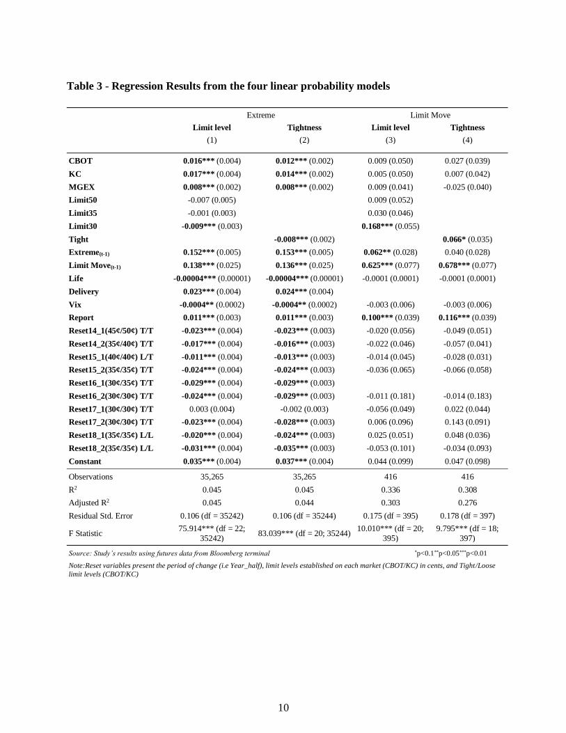
negative impact on the extreme movement likelihood and were statistically significant. displays

the estimated likelihood of extreme movements from model 1 using control (Paris) and all other

three market data on a six months average basis. The period before 2014 is our reference for

comparison since it was excluded from our models to avoid singularity issures.

3

In early 2014, the limit levels reset from 60 cents to 45. This considerable reduction (tighter limit

level) impacted negatively the probability of extreme movements in comparison to the period

before when price limits were static. According to our models the first 2014 reset window

coefficient is one of the largest ones in magnitude. We observed a considerable decrease in the

probability of extreme movements for both control and markets from the first 2015 reset window

until late 2016 in comparison with the static period which consists of tight reset windows with

negative statistically significant coefficients. The first 2017 reset window (Positive coefficient)

indicates a period when the probability of extreme move would return to similar levels as the

static period (before 2014) as Figure 2 shows. Those levels would be significantly greater

(approximally 3.5%) than our data baseline of 0.24% for Paris (Control) and 1.4% for the other

markets on average in daily terms, however not statistically significant

The next period of tighter reset windows occurred from late 2017 until late 2018 with an

ambiguous behavior. Late 2017, the daily limit stayed at the same level as of late 2016, however,

this period shows the higher probability levels only reducing late 2018. In this period is clear to

see the difference in reaction over Paris and other markets. The level’s magnitude and how sharp

is the response in CBOT, KC, and MGEX can be seen through this period. The results from the

first models are aligned with the Holding back hypothesis (Subrahmanyam 1997) that price limit

helps to decrease volatility which in our analysis can be observed as a contraction in the

probability of extreme movements. Brogaard and Roshak (2015) conclude that circuit breaks

such as price limit can improve market stability by decreasing large movements and our present

results so far can lead us to a similar conclusion. However, some trade-off would probably be

involved to acquire this stability, such as a reduction in price discovery.

The next two models estimate the probability of a limit move given the occurrence of an extreme

movement. The same description of the first two models applies to those, where we use the limit

levels variable and tightness. Our third model overall presents an Adjusted R-squared of 0.303

and a global F test significant at a 1% level. With a better goodness-of- fitness relative to the past

models, the 30-cent limit level coefficient presented statistically significant at 1% with a

relatively large positive effect on the probability of a limit move (0.168% increase over a 0.05%

overall baseline). The result is intuitive. Since 30 cents is the most restrictive limit level in our

limit level historical series it is logical to show an increment in the probability of limit move

4

given extreme movements. However, considering that our coefficient is based relative to our

control (Paris), we can assume that the positive marginal effect on the conditional probability of

a limit move supports the Magnetism hypothesis (Subrahmanyam (1994), Chan et.al. (2005) and

Treynor, (2019)). Another powerful insight is regarding the Lag Limit move variable. This

variable gives a hindsight on the probability of a limit move that could help market participants

to place their orders and strategies. The occurrence of a limit move on the previous day increase

the probability by 0.678% with a base line of 0.05%.

The last model considers tightness. It presents an Adjusted R-square of 0.276 and a global F test

statistically significant at 1% level. Besides present a lower goodness-of-fit, the variable Tight is

significant at 1% level and corroborates with the conclusion observed for the third model where

the Magnet hypothesis is supported since it counts for all restriction increase throughout all limit

level.

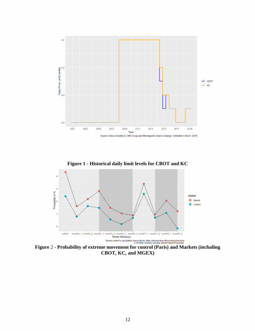
Figure 3 displays the estimated probability of limit moves conditional to extreme movements

occurrence in MGEX, KC, and CBOT using model 4 due to the tight variable presence. The

same periods from Figure 2 are highlighted and the coefficient effects are only valid for

comparions throughout the period analyzed. We find opposite results from our first two models

observing the shaded area from the first reset window in 2015 to second in 2016. This period

presents limit levels with negative marginal effects on the probability of extreme moves on the

first two models, however, our estimates for the probability of limit moves conditional to

extreme moves increase in those periods. Those tight windows marginal increments on the

probability of a limit move after the occurrence of an extreme move corroborate with the

“Magnet” hypothesis taking limit moves as a proxy for volatility. Paris was not displayed

because the probability of hit the limit is always zero (since it is our control).

The second period highlighted from late 2017 to late 2018 shows a loose limit level. The last two

windows were classified as loose since the limit level starts to get wider (from 30 cents to 35 for

both Chicago and KC contracts). Even with negative effects on the coefficients, the probability

of limit moves drastically drops on this period which empirically still corroborates with our

positive relationship between tightness and probability of limit moves conditional to extreme

moves. This section of our series supports the Magnetism hypothesis and is aligned with our

regression results for model 4 where a tight limit level increases the probability of limit move

(loose limit level decrease probability of limit move).

Our findings on the second probability estimation regarding limit move conditional to extreme

movement occurrence support the Magnetism hypothesis in a certain way, where tighter limit

levels increase the probability of a limit move. It is known that our sample size for limit moves

conditional to extreme movements is small (416 observations) and only 19 days where price

reached the limit threshold. Etienne, Irwin, and Garcia (2015) evaluate price explosiveness on

corn, soybeans and wheat futures markets from 2004-2013. On their findings, only 2% of the

whole sample experience a price explosive moment and, regarding wheat contracts, only ten,

twenty-five and twenty-seven business days had price explosiveness for CBOT, Kansas City and

Minneapolis contracts. Their conclusion reinforces how rare those events are but still could

generate substantial implications for the market.

Ex-post effects

5

The ex-post effects of price limits are evaluated in this study by observing trading volume during

limit days and through the use of an estimated counterfactual for trading volume in that market-

contract-day, infer price limit effects on trading volume.

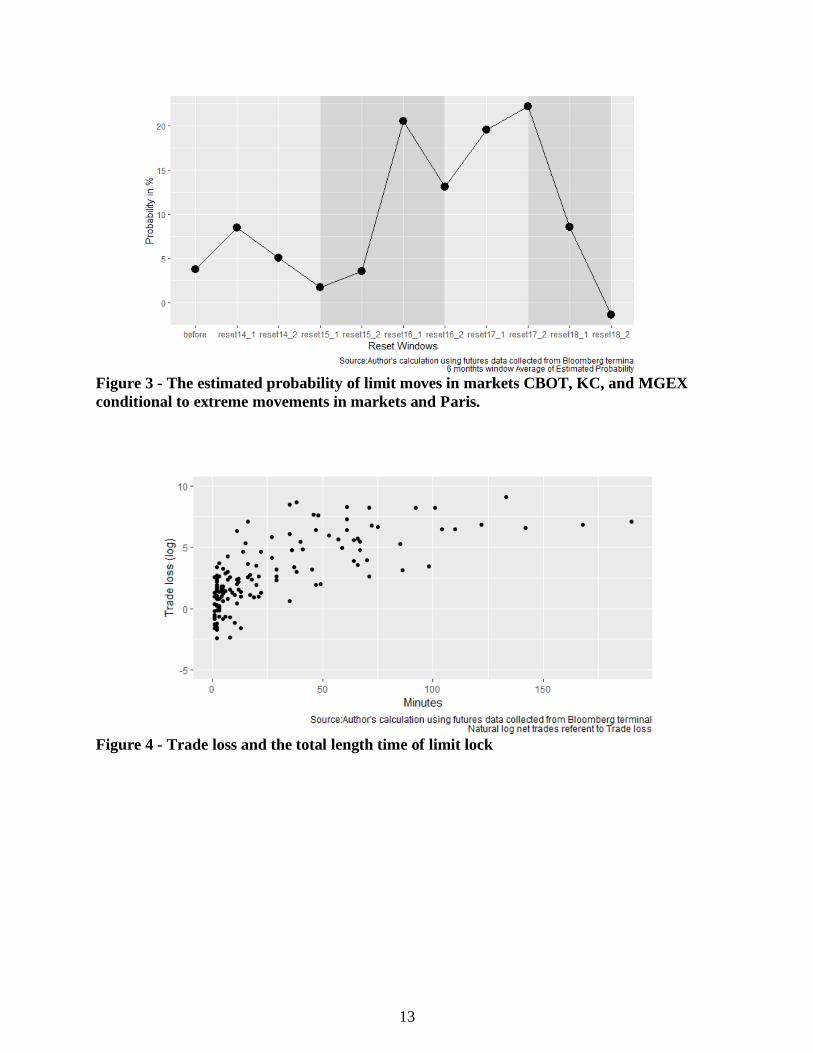
To better understand our results, the first step is to evaluate the duration of all limit moves

observed in our data sample against net trade, which is the difference between our adjusted

counterfactual volume and the actual volume at the limit move day and is expressed by the

variable Min.lock. shows the ex-post data summary statistics. The greater sum of minutes with

price locked at the limit level is 190 and is related with a max net trade loss of approximally

9200 contracts. For net trade gains, the data shows a max sum of minutes equals to 164. Our data

shows a greater number of observations where net trade gains happened in comparison with net

trade loss, but the max net trade loss (9159 contracts) is greater than the max net trade gain (3576

contracts) observed.

To better understand this relationship between limit lock duration and net trade behavior those

two dimensions are displayed in Figure 4 and Figure 5 for trade losses and gains. For both, it is

possible to observe a positive relationship between long periods of limit locks and trade gains

and losses, however, this behavior is more evident for trade losses. It is worth mentioning that

this relationship seen in those figures are not for a continuous limit lock but by the total sum of

minutes that prices stayed at the limit level. Observing the data, we notice different trading

activity responses according to how long and if there were gaps within limit locks.

Trading volume doesn’t respond immediately to a limit hit. Volume tends to shift around a limit

hit where a peak is evident before prices bind with the limit taking a moment to reduce to lower

levels. This delay effect of price limits on trading volume could restate the classical U-shaped

volume curve inside a trading session where a volume peaks would be seen around a limit hit

and another one right after prices come back to the range. To investigate this effect, enlights the

subject. Our five models are displayed in the table where the first, second and third are

implemented with levels of net trade as our dependent variable. The last two use the natural

logarithm aiming more comprehensible coefficients.

All models present an F statistic significant at 1% level. All models presented a fair goodness-of-

fit with the higher adjusted R2 for model 2 (0.422) and lowest for model 1 (0.116). Among the

level models, Min.lock coefficient presented statistically significant at 1%. The marginal effect

of an extra minute locked at the limit level is positive for both trade loss and gain, however, on

average its impact is greater for losses (26 contracts for an additional minute locked at the limit

level). Moreover, the overall model using net trade variable as a linear variable (accounting for

positive (trade losses) and negative (trade gains)) shows a positive marginal effect for Min.lock

which increases trading activity loss by approximately 13 contracts for an additional minute. The

same conclusion can be seen from our Log-level models. The marginal effect of an additional

minute in the sum of minutes where prices stay at the limit level increase more trading activity

losses (6.1% for an additional minute) than trading activity gains (2.3% for an additional

minute).

The delay effect of price limits can be explained through the Gap coefficient. Empirically we can

see that short limit locks our limit days with large gaps show the occurrence of a U-shaped

pattern in the volume curve. Practically, the peak in volume due to a limit hit is not compensated

by the halt on trading activity if prices would stay locked at limit levels. The coefficients of our

level models show this. The longer the gap, the greater is trading activity gain.

6

In the level models, the marginal effect of an additional minute for the gaps increases trading

activity gains. In the trade loss model, an additional minute in the gap reduces trade loss by 0.868

contracts and in the trade gain model, 0.281 contracts. In our log-level models, the results are in

the opposite direction where an additional minute in the gap between limit hits reduces trading

activity gains by 1%. One reason for the increment in trading activity could be that non-

commercial traders reduce their net short and net long positions when an upper and lower limit

gets hit to cover their margin calls (Janardanan et.al., 2019).

The intensity of gains and losses on trading activity are different according to our model. The

Kansas City interaction variables KC_Min.lock and KC_gap help to understand the different

intensities the effect of our variables of interest have on both markets. To obtain the effect of an

extra minute locked at the limit and the effect of an extra minute in a gap for Kansas City we

need to calculate the sum of Min.Lock and Gap coefficient and the interaction coefficients,

respectively. In this case, the marginal effect of an extra limit locked at the limit in Kansas City

is relatively small (approximately 3 contracts) to Chicago. The same conclusion can be seen for

the gap interaction variable. Overall, a gap between limit hits increase trading activity gains.

However this effect is lower in Kansas City relative to Chicago due to the sum of coeffients (Gap

and KC_Gap) being almost zero. A reasonable evidence to support this result is the difference in

magnitude of trade gains and losses observed on both markets. Figure 6 illustrate this difference

in magnitude by displaying the amount of minutes locked at the limit versus trade gains and

losses. Clearly, CBOT values for trade gains and losses are fairly greater than KC showing that

by the fact that CBOT wheat contracts presenting a higher volume on average compared with

KC makes the effect of limit move on trading activity more intense in CBOT. The same pattern

can be seen for gap values.

7

Conclusions

In this study, we use future price and volume data from the four major wheat futures markets,

Chicago , Kansas City, Minneapolis, and Paris to estimate the ex-ante and ex-post effects of

price limits. We estimate the impact of changing price limits on the probability of extreme

movements and the probability of limit moves conditional on the occurrence of extreme

movements similar to Brogaard and Roshak (2015). For the ex-post effects, we investigate how

trading activity behaves before, during and after a limit hit.

In our ex-ante assessment, the results indicate that tighter limit levels decrease the probability of

extreme movements by 0.008% with a baseline probability of 1.11% for all four markets studied.

In essence, exchanges with the procedure to revise their limit levels periodically, when revised to

a tighter level, on average reduce the probability of extreme movements based on the results

generated by the period analyzed in this study. These findings support the “Holding Back”

hypothesis suggested by Subrahmanyam (1997) with the caveat that extreme movements have to

be used as a proxy for volatility. However, our estimate for the probability of a limit move

conditional to extreme movements points the contrary. Logically, tighter limit levels increase the

probability of limit moves when extreme moves happen which supports the “Magnet” hypothesis

implied by Subrahmanyam (1994) when we confront the results with our control (Paris) where

price limits do not apply. Moreover, the occurance of a limit move on the day before could be

used as a hindsight information since the marginal effect of our Lag Limit move is positive and

relatively larger when compared with our base line for limit move (0.05%)

The ex-post effects of price limit on trading activity are consistent with our empirical

investigation. Trading activity has a unique behavior when prices are about to hit the limit where

a U-shaped volume curve traditionally observed in a trading session can repeat itself. This

behavior is subject most by how long prices will stay at the limit level and/or if prices will hit the

limit level multiple times in a session. Our results indicate that the longer is the period where

prices are at the limit, the greater is the trading activity loss in comparison with a possible trading

activity gain. Moreover, if prices hit the limit level multiple times in a session and the time

between hits is longer, the trading session can experience an increase in trading activity. The

intensity of those effects change through markets as well. Due to its lower daily volume

compared with Chicago, Kansas City react less to ex-post effects relative to Chicago.

The results could help market participants by increasing their information regarding the effects

of this rare market events and help them navigate efficiently through the commodity markets.

For policymakers and exchanges, this study could enlighten more information about price limit

effects on price and trading activity thus supporting them to implement these circuit breaks

effectively.

Further researches could collaborate with the subject by evaluating intraday datasets with higher

resolutions and for other markets where price limits are constantly hit it and that could show

inefficient such as Live Cattle and Lumber. Moreover, evaluating the behavior of order in the

order book could increment the analysis and clarify price limit effects.

8

References

Admati, A. R. ., & Pfleiderer, P. (1988). A theory of Intraday Patterns: Volume and Price

Variability. Financial Studies, 1(1), 3–40.

Brogaard, J., & Roshak, K. (2015). Prices and Price Limits. Ssrn, (June 2015).

https://doi.org/10.2139/ssrn.2667104

Chan, S. H., Kim, K. A., & Rhee, S. G. (2005). Price limit performance: Evidence from

transactions data and the limit order book. Journal of Empirical Finance, 12(2), 269–290.

https://doi.org/10.1016/j.jempfin.2004.01.001

Etienne, X. L., Irwin, S. H., & Garcia, P. (2015). Price explosiveness, speculation, and grain futures

prices. American Journal of Agricultural Economics, 97(1), 65–87.

https://doi.org/10.1093/ajae/aau069

Hautsch, N., & Horvath, A. (2019). How effective are trading pauses? In Journal of Financial

Economics (Vol. 131). https://doi.org/10.1016/j.jfineco.2017.12.011

Janardanan, R., Qiao, X., & Rouwenhorst, K. G. (2019). On commodity price limits. Journal of

Futures Markets, 39(8), 946–961. https://doi.org/10.1002/fut.21999

Ma, C. K., Rao, R. P., & Sears, R. S. (1989). Volatility, price resolution, and the effectiveness of

price limits. Journal of Financial Services Research, 3(2–3), 165–199.

https://doi.org/10.1007/BF00122800

Reiffen, D., Buyuksahin, B., & Haigh, M. S. (2011). Do Price Limits Limit Price Discovery in the

Presence of Options? SSRN Electronic Journal. https://doi.org/10.2139/ssrn.928013

Subrahmanyam, A. (1997). The ex ante effects of trade halting rules on informed trading strategies

and market liquidity. Review of Financial Economics, 6(1), 1–14.

https://doi.org/10.1016/S1058-3300(97)90011-2

Subrahmanyam, A. (1994). Circuit Breakers and Market Volatility: A Theoretical Perspective. The

Journal of Finance, 49(1), 237–254. https://doi.org/10.1111/j.1540-6261.1994.tb04427.x

Treynor, J. L. (2019). What Does It Take To Win The Trading Game ? Financial Analysts Journal,

37(1), 55–60.

9

Table 1 - Extreme and limit move descriptive statistics for the wheat futures market

Table 2 - Ex-post data summary statistics

Variable Mean or % Sum Mean or % Sum Mean or % Sum Mean or % Sum Mean or % Sum

Regular Moves 92.76% 34863 92.33% 9668 91.99% 8709 93.40% 8062 99.66% 8424

Extreme Moves 1.11% 416 1.21% 127 1.40% 133 1.47% 127 0.32% 29

Limit Moves 0.05% 19 0.09% 9 0.10% 9 0.01% 1 0.00% -

Limit 60 76.04% 26826 100.00% 9795 100.00% 8842 100.00% 8189 0.00% -

Limit 50 49.09% 17320 92.91% 9101 92.95% 8219 0.00% - 0.00% -

Limit 35 36.66% 12933 73.35% 7185 65.01% 5748 0.00% - 0.00% -

Limit 30 16.27% 5739 31.01% 3037 30.56% 2702 0.00% - 0.00% -

N 35279 - 26.06% 9795 25.06% 8842 21.79% 8189 22.49% 8453

Full Sample CBOT KC MGEX EBM

Variable Sum Sum Sum

Max min. lock 190 190 164

Min min. lock 1 1 1

Median min. lock 14 11 15

Average min. lock 24.69 26.98 23.36

Max Gap 1128.67 1128.67 1101.92

Min Gap 0 0 0

Median Gap 48.87 37 57.6

Average Gap 122.01 131.47 117.56

Max Net trade 9159.27 9159.27 3576.13

Min Net trade -3576.13 0.001 0.001

Median Net trade -9.1 9.02 50.63

Average Net trade 0.95 382.2 218

N 392 143 249

Full Sample Trade Loss Trade Gain

10

Table 3 - Regression Results from the four linear probability models

Extreme Limit Move Limit level Tightness Limit level Tightness (1) (2) (3) (4)

CBOT 0.016*** (0.004) 0.012*** (0.002) 0.009 (0.050) 0.027 (0.039)

KC 0.017*** (0.004) 0.014*** (0.002) 0.005 (0.050) 0.007 (0.042)

MGEX 0.008*** (0.002) 0.008*** (0.002) 0.009 (0.041) -0.025 (0.040)

Limit50 -0.007 (0.005) 0.009 (0.052)

Limit35 -0.001 (0.003) 0.030 (0.046)

Limit30 -0.009*** (0.003) 0.168*** (0.055)

Tight -0.008*** (0.002) 0.066* (0.035)

Extreme(t-1) 0.152*** (0.005) 0.153*** (0.005) 0.062** (0.028) 0.040 (0.028)

Limit Move(t-1) 0.138*** (0.025) 0.136*** (0.025) 0.625*** (0.077) 0.678*** (0.077)

Life -0.00004*** (0.00001) -0.00004*** (0.00001) -0.0001 (0.0001) -0.0001 (0.0001)

Delivery 0.023*** (0.004) 0.024*** (0.004)

Vix -0.0004** (0.0002) -0.0004** (0.0002) -0.003 (0.006) -0.003 (0.006)

Report 0.011*** (0.003) 0.011*** (0.003) 0.100*** (0.039) 0.116*** (0.039)

Reset14_1(45¢/50¢) T/T -0.023*** (0.004) -0.023*** (0.003) -0.020 (0.056) -0.049 (0.051)

Reset14_2(35¢/40¢) T/T -0.017*** (0.004) -0.016*** (0.003) -0.022 (0.046) -0.057 (0.041)

Reset15_1(40¢/40¢) L/T -0.011*** (0.004) -0.013*** (0.003) -0.014 (0.045) -0.028 (0.031)

Reset15_2(35¢/35¢) T/T -0.024*** (0.004) -0.024*** (0.003) -0.036 (0.065) -0.066 (0.058)

Reset16_1(30¢/35¢) T/T -0.029*** (0.004) -0.029*** (0.003)

Reset16_2(30¢/30¢) T/T -0.024*** (0.004) -0.029*** (0.003) -0.011 (0.181) -0.014 (0.183)

Reset17_1(30¢/30¢) T/T 0.003 (0.004) -0.002 (0.003) -0.056 (0.049) 0.022 (0.044)

Reset17_2(30¢/30¢) T/T -0.023*** (0.004) -0.028*** (0.003) 0.006 (0.096) 0.143 (0.091)

Reset18_1(35¢/35¢) L/L -0.020*** (0.004) -0.024*** (0.003) 0.025 (0.051) 0.048 (0.036)

Reset18_2(35¢/35¢) L/L -0.031*** (0.004) -0.035*** (0.003) -0.053 (0.101) -0.034 (0.093)

Constant 0.035*** (0.004) 0.037*** (0.004) 0.044 (0.099) 0.047 (0.098)

Observations 35,265 35,265 416 416

R2 0.045 0.045 0.336 0.308

Adjusted R2 0.045 0.044 0.303 0.276

Residual Std. Error 0.106 (df = 35242) 0.106 (df = 35244) 0.175 (df = 395) 0.178 (df = 397)

F Statistic 75.914*** (df = 22;

35242) 83.039*** (df = 20; 35244)

10.010*** (df = 20;

395)

9.795*** (df = 18;

397)

Source: Study’s results using futures data from Bloomberg terminal *p<0.1**p<0.05***p<0.01

Note:Reset variables present the period of change (i.e Year_half), limit levels established on each market (CBOT/KC) in cents, and Tight/Loose

limit levels (CBOT/KC)

11

Table 4 - Regression results from ex-post effect model designs

Nominal Logarithm All Data Trade Loss Trade Gain Log Trade Loss Log Trade Gain (1) (2) (3) (4) (5)

Min.lock 12.952*** 26.371*** 5.251*** 0.061*** 0.023* (1.940) (3.475) (1.346) (0.014) (0.014)

KC_Min.lock -12.566*** -23.841*** -3.470 0.009 0.118*** (3.626) (6.283) (2.423) (0.026) (0.025)

Gap -1.199*** -2.542*** 0.827*** -0.003 0.002 (0.323) (0.639) (0.195) (0.003) (0.002)

KC_Gap 1.165*** 2.612*** -0.847*** 0.005 -0.023***

(0.418) (0.797) (0.260) (0.003) (0.003)

Total Vol 0.007*** 0.015*** 0.001 0.00002** 0.00000 (0.002) (0.003) (0.001) (0.00001) (0.00001)

KC 219.389** -124.499 -85.338 -2.416*** -2.394*** (108.456) (199.271) (70.921) (0.811) (0.741)

Extreme(t-1) -2.146 -190.114 -132.468* -1.181 -0.648 (126.212) (261.731) (74.493) (1.065) (0.779)

Vix 0.780 6.636 -0.538 0.005 -0.033 (4.579) (11.389) (2.586) (0.046) (0.027)

Report -132.911 -256.530 -50.517 0.204 -0.863 (143.444) (338.580) (81.563) (1.378) (0.853)

Life 3.168** 6.135** 0.348 0.006 -0.010 (1.411) (2.365) (0.954) (0.010) (0.010)

Constant -709.153*** -981.101*** 82.689 0.643 4.975*** (192.715) (372.052) (124.820) (1.514) (1.305)

Observations 392 143 249 143 249

R2 0.139 0.463 0.263 0.330 0.429

Adjusted R2 0.116 0.422 0.232 0.280 0.405

Residual Std. Error

792.546 (df = 381) 894.224 (df = 132) 388.033 (df = 238) 3.640 (df = 132) 4.057 (df = 238)

F Statistic 6.137*** (df = 10;

381) 11.378*** (df = 10;

132) 8.481*** (df = 10;

238) 6.511*** (df = 10;

132) 17.914*** (df = 10;

238)

Source: Study’s results using futures data from Bloomberg terminal and CQG intraday data *p<0.1**p<0.05***p<0.01 Notes: Trade loss and Trade gain are distinguished by the sign. Net trade positive values are trade loss and negative values are gain

12

Figure 1 - Historical daily limit levels for CBOT and KC

Figure 2 - Probability of extreme movement for control (Paris) and Markets (including

CBOT, KC, and MGEX)

13

Figure 3 - The estimated probability of limit moves in markets CBOT, KC, and MGEX

conditional to extreme movements in markets and Paris.

Figure 4 - Trade loss and the total length time of limit lock

14

Figure 5 - Trade gain and the total length time of limit lock

Figure 6 - Trade gains and losses for Chicago and Kansas City contracts in nominal level

(contracts)