Evolving optimum populations with XCS classifier systems

ORIGINAL PAPER

Evolving optimum populations with XCS classifier systems

XCS with code fragmented action

Muhammad Iqbal • Will N. Browne •

Mengjie Zhang

Published online: 30 September 2012

� Springer-Verlag 2012

Abstract The main goal of the research direction is to

extract building blocks of knowledge from a problem

domain. Once extracted successfully, these building blocks

are to be used in learning more complex problems of the

domain, in an effort to produce a scalable learning classi-

fier system (LCS). However, whilst current LCS (and other

evolutionary computation techniques) discover good rules,

they also create sub-optimum rules. Therefore, it is difficult

to separate good building blocks of information from oth-

ers without extensive post-processing. In order to provide

richness in the LCS alphabet, code fragments similar to

tree expressions in genetic programming are adopted. The

accuracy-based XCS concept is used as it aims to produce

maximally general and accurate classifiers, albeit the rule

base requires condensation (compaction) to remove spuri-

ous classifiers. Serendipitously, this work on scalability of

LCS produces compact rule sets that can be easily con-

verted to the optimum population. The main contribution

of this work is the ability to clearly separate the optimum

rules from others without the need for expensive post-

processing for the first time in LCS. This paper identifies

that consistency of action in rich alphabets guides LCS to

optimum rule sets.

Keywords Learning classifier systems � XCS �Optimal populations � Scalability � Code fragments �Action consistency

1 Introduction

Human beings have the ability to apply the domain

knowledge learned from a smaller problem to more com-

plex problems of the same or a related domain, but cur-

rently machine learning techniques lack this ability. This

lack of ability to apply the already learned knowledge of a

domain results in consuming more resources and time to

solve more complex problems of the domain. As the

problem scales, it becomes difficult and even sometimes

impractical (if not impossible) to solve due to the needed

resources and time.

Therefore, a system is needed that has the ability to

reuse the learned knowledge of a problem domain to scale

in the domain. If the system has modularity and coopera-

tion among the modules, it can help to reuse the knowledge

effectively using an evolutionary mechanism. A learning

classifier system (LCS) is an evolutionary adaptive system

that learns a problem using a set of rules cooperating

among each other (Holland 1986), whereas most of the

traditional evolutionary techniques have competition only

among the individuals.

Typically, an LCS represents a rule-based agent that

incorporates evolutionary computing and machine learning

to solve a given task. The rules are of the form ‘‘if state

then action’’. An LCS learns by interacting with the

environment. Typically, it starts learning by covering the

individual data patterns given as input from the environ-

ment in rules, such as ‘100110 : 1’, i.e. if input is ‘100110’

then the action will be ‘1’. It generalizes the population of

M. Iqbal (&) � W. N. Browne � M. Zhang

School of Engineering and Computer Science,

Victoria University of Wellington,

Wellington 6140, New Zealand

e-mail: [email protected]

W. N. Browne


M. Zhang


123

Soft Comput (2013) 17:503–518

DOI 10.1007/s00500-012-0922-5

classifiers by attempting to remove irrelevant information.

Usually, the generality is achieved using the common ter-

nary alphabet {0, 1, #} where ‘#’ is the ‘don’t care’ symbol

that can be either 0 or 1, e.g. ‘10##1#:1’.

The LCS technique can scale in problem domains, but

has to relearn from the start each time. Further, increased

dimensionality of the problem, resulting in increased

search space, demands large memory space and leads to

much longer training times; and eventually restricts the

LCS to a limit in problem size. By explicitly feeding

domain knowledge to an LCS, scalability can be achieved

but it adds bias and restricts use in multiple domains

(Ioannides and Browne 2007). On the other hand, human

beings learn the underlying method to construct a solution,

and so can scale the problem arbitrarily.

The main goal of the research direction is to develop an

LCS capable of autonomously scalable learning, from

small problems to more complex problems of the same or a

related domain, in a similar behavior to human beings

(Thrun 1996). A modular approach to learning in LCS is to

be adopted so that building blocks of knowledge may be

formed and utilized. It is anticipated that the modular

approach will make the system more scalable. The rela-

tively fitter modules from a learning system trained against

a small problem will be put in a higher level problem in the

same or a related domain to reduce the learning time of the

system.

In order to extract building blocks of knowledge in the

form of reusable modules or functions, a richer encoding

scheme will be used in the work presented here. In this

encoding representation, the action will be replaced by a

code fragment while using the typical ternary alphabet for

the condition of a classifier. A code fragment is a tree

expression, similar to a tree generated in genetic pro-

gramming (see Sect. 2.2).

Wilson’s accuracy-based XCS (Wilson 1995), the most

popular learning classifier system, is used to implement and

test the proposed system. It is a well studied and tested

‘‘non-supervised reinforcement (learning)’’ learning clas-

sifier system. In XCS the genetic algorithm is applied to an

action set instead of the whole population to conserve

similar building blocks of information. These features of

XCS make it possible to form a complete and accurate

mapping from inputs and actions to payoff predictions. The

ability of XCS to produce complete and accurate solution,

for a given problem, motivated its suitability for this

research work. If a learning system is unable to produce a

complete and accurate solution, then the extracted building

blocks lack important knowledge. These building blocks,

missing vital knowledge, are not suitable candidates to be

used for scalability of the system.

Serendipitously, this work on scalability of LCS pro-

duced compact rule sets that were easily converted to the

optimum population. Where alternative good rules were

discovered, the most condensed were selected. The aim of

this paper is to detail and investigate this novel approach in

LCS to determine the mechanism by which optimum

solutions for the given setup are produced. Once the

method for successful learning has been determined, this

technique will be applied to a broad range of problems, but

this work is beyond the scope of this paper.

The rest of the paper is organised as follows. Section 2

describes genetic algorithm, building blocks, genetic pro-

gramming, learning classifier systems and accuracy-based

learning classifier systems. In Sect. 3, the novel imple-

mentation of XCS using code fragmented actions is

detailed. Section 4 introduces the multiplexer problem

domain and experimental setup used in the experimenta-

tion. In Sect. 5, experimental results are presented and

compared with standard implementation of XCS using

static binary actions. Section 6 is discussion, elaborating

action consistency and production of the optimum solution.

In the last section, this work is concluded and the future

work is outlined.

2 Background

Evolutionary computational techniques (Eiben and Smith

2003; Jong 2006) are based on the ideas of Darwin’s theory

of survival of the fittest. An evolutionary process starts with

a population of, usually randomly generated, individuals

where each individual represents a potential problem

solution or a part of the solution. Each individual is eval-

uated to determine its utility or fitness for the given

problem. Relatively fit members of the population are

selected to create new offspring and the worst members

may be deleted from the population. This process of evo-

lution is repeated for a fixed number of times or until an

ending criterion is met.

In the following subsections, two of the most common

evolutionary techniques namely genetic algorithms and

genetic programming are briefly described, as they are

directly related to the work presented here. This is followed

by an introduction to learning classifier systems.

2.1 Genetic algorithms and building blocks

The discovery component of an LCS is commonly imple-

mented using a genetic algorithm (GA). An LCS seeks to

evolve a population of co-operative rules, where each

individual rule is optimized using the GA.

GAs are population-based search algorithms (Holland

1975) where each individual member of the population

is usually represented by a bitstring of finite length. A

population of randomly generated individuals, each

504 M. Iqbal et al.

123

representing a potential problem solution, is used at the

start. After that, each individual is evaluated to determine

its utility or fitness for the given problem. Then, new

populations are generated and evaluated, using genetically

inspired operations of reproduction, crossover and muta-

tion. The individuals are probabilistically selected to par-

ticipate in the genetic operations based on their fitness.

Reproduction is a process in which the selected individual

strings are simply copied to the new generation, i.e. sur-

vival of the fittest individuals. In the crossover operation,

two new individuals are generated by swapping elements

of two or more, hypothesized the best, selected individuals.

Mutation operates at the bit level by randomly flipping bits

within the current individual. This process of evolution is

repeated for a fixed number of times or until an ending

criterion is met. The fittest individual in the final popula-

tion is taken as the solution to the problem. GAs are purely

competitive with the whole population aiming to converge

to the optimal solution, whereas LCSs are competitive only

in niches, i.e. separable subsolutions of the problem

domain that when combined cover the complete space of

the problem.

To better understand the behavior and performance of

genetic algorithms in any evolutionary system, Goldberg

(Goldberg 1989) has studied and described a GA using the

concept of schema. A schema is a similarity template for

describing a set of finite-length strings defined over a finite

alphabet. For example, if the alphabet is {0, 1, *} then the

schema ‘‘1**0’’ is describing all strings of length four that

start with symbol 1 and end with symbol 0 such as 1000,

1010, 1100, and 1110. It is to be noted that ‘*’ is treated as

‘don’t care’ symbol here, meaning it can be either 0 or 1.

The distance between first and last specific string positions

in a schema H is called its defining length, denoted by

d(H), and the number of specific positions in it is called its

order, denoted by o(H). For example the defining length of

the schema ‘‘1**0’’ is 3 and the order is 2, whereas the

defining length of the schema ‘‘101*’’ is 2 and the order is 3.

Goldberg hypothesized that higher performance indi-

viduals are actually generated as a result of the combina-

tion of short-length, low-order and high-performance

schemata (Goldberg 1989). These schemata are called the

building blocks of the system. These building blocks are

likely to be selected and combined via crossover to produce

longer and fit individuals in a GA. These building blocks

are also relatively less affected by mutation. The assump-

tion by Goldberg that this is the way how a GA works, is

termed the building block hypothesis.

However, for a population of individuals represented by

fixed length strings, the genetic operators sometimes can-

not process the building blocks effectively as a random

crossover point may lie within the building block. To avoid

this disruption of partial solutions by the genetic operators,

a probability distribution-based approach, known as Esti-

mation of Distribution Algorithm (EDA), was developed

(Mhlenbein and Paaß 1996). In the various forms of EDAs,

the crossover and mutation operators are replaced by

generating new offspring according to the probability dis-

tribution of the selected individuals (Pelikan et al. 2002).

A sample from a schema such as ‘‘1**0’’ is implicitly

sampling from many other schemata too, like ‘‘10*0’’,

‘‘11*0’’, ‘‘1*00’’, and ‘‘1*10’’. It has been estimated that in

any generation of a population of n individuals, the number

of schemata being processed by the GA is proportional to

n3. This inherently parallel processing of a large quantity of

schemata is known as implicit parallelism.

The schema theory has been criticized due to its weak

theoretical foundations (Altenberg 1995; Beyer 1997;

Burjorjee 2008), but still remains a popular tool to explain

the power of GAs (Poli and Langdon 1998; Poli 2000;

Drugowitsch 2008).

2.2 Genetic programming

Commonly, genetic programming (GP) uses a much richer

alphabet than GA to encode the solution, i.e. more

expressive symbols that can express functions as well as

numbers. A GP like alphabet to describe the problem is

used in the LCS developed here, so the GP technique is

described to aid understanding.

GP is an evolutionary approach to generating computer

programs for solving a given problem automatically (Koza

1992; Banzhaf et al. 1998; Poli et al. 2008). GP is an

extension of the GA in which the structures in the popu-

lation are not fixed-length character strings that encode

candidate solutions to a problem, but programs that, when

executed, generate the candidate solutions to the problem.

The task to be solved is represented by a primitive set of

operations, known as the function set, and a set of oper-

ands, known as the terminal set. The generated computer

programs are commonly represented by a tree. The internal

nodes of the tree are functions and leaves are the terminals.

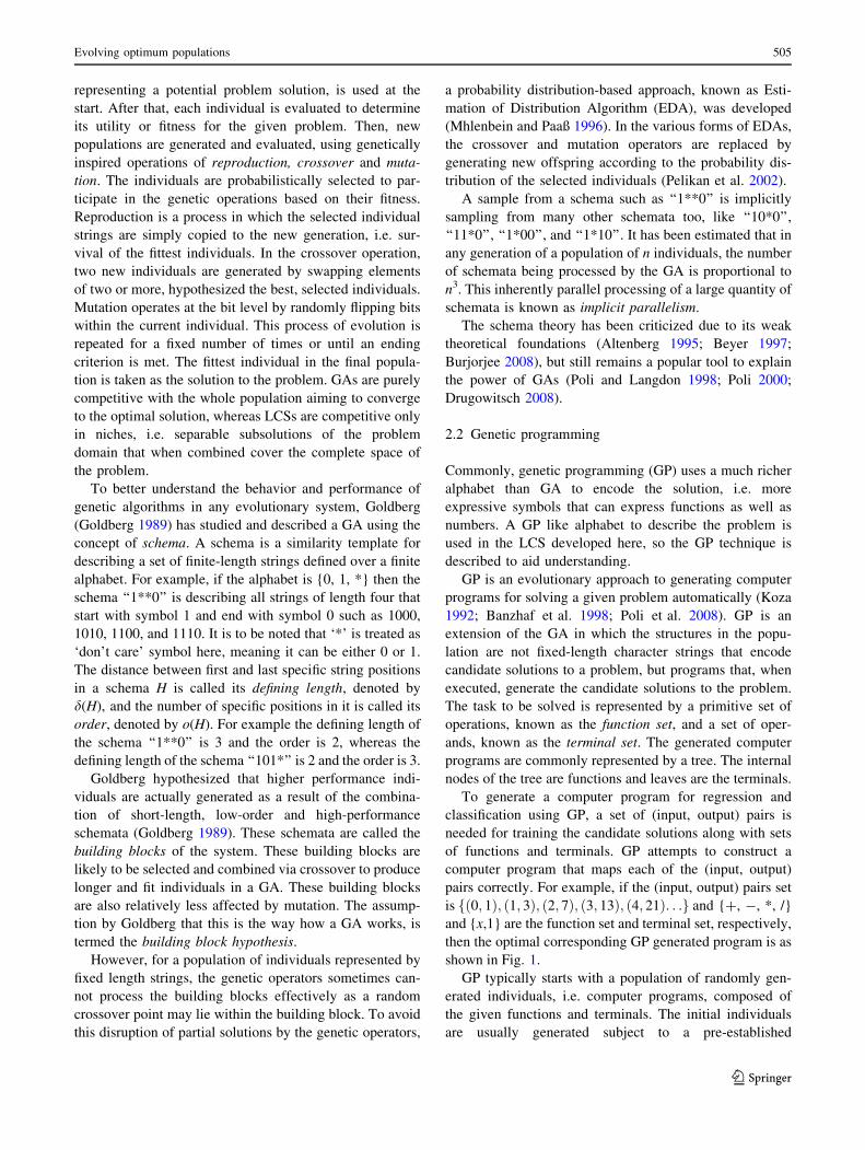
To generate a computer program for regression and

classification using GP, a set of (input, output) pairs is

needed for training the candidate solutions along with sets

of functions and terminals. GP attempts to construct a

computer program that maps each of the (input, output)

pairs correctly. For example, if the (input, output) pairs set

is fð0; 1Þ; ð1; 3Þ; ð2; 7Þ; ð3; 13Þ; ð4; 21Þ. . .g and {?, -, *, /}

and {x,1} are the function set and terminal set, respectively,

then the optimal corresponding GP generated program is as

shown in Fig. 1.

GP typically starts with a population of randomly gen-

erated individuals, i.e. computer programs, composed of

the given functions and terminals. The initial individuals

are usually generated subject to a pre-established

Evolving optimum populations 505

123

maximum size (Koza and Poli 2005). GP iteratively

transforms a population of computer programs into a new

generation of the population by applying the genetic

operations of reproduction, crossover and mutation to

selected individuals from the population. The individuals

are probabilistically selected to participate in the genetic

operations based on their fitness. Reproduction involves

simply copying certain individuals into the new population.

Given copies of two parent trees, typically, crossover

involves randomly selecting a crossover point in each

parent tree and swapping the sub-trees rooted at the

crossover points. Traditional mutation consists of randomly

selecting a mutation point in a tree and substituting the sub-

tree rooted there with a randomly generated sub-tree. This

process of evolution is repeated for a fixed number of times

or until an ending criterion is met. The fittest individual

program in the final population is used to compute the

solution to the problem.

GP is a technique that can produce a computer pro-

gram automatically to maximally map an (input, output)

pairs set. However, to generate this program it needs

many CPU cycles and much memory space (Robilliard

et al. 2009). The GP-generated computer program is

normally represented as a tree, which may contain

unnecessary terms (bloat) and non-optimum expressions

(a phenotypic behavior may not be represented by the

most compact genotype). These problems are usually

addressed by limiting maximal allowed depth for an

individual tree and/or using a fitness measure that pun-

ishes excess sized individuals (Luke and Panait 2006).

The other ways to control bloat in genetic programing

include simplifying individual programs using algebraic

and numerical simplification methods (Kinzett et al.

2009), or using specific bloat control operators (Alfaro-

Cid et al. 2010).

A GP system produces a tree as a ‘single’ solution,

rather than a co-operative set of rules as in an LCS. It

generally requires supervised learning (Russell and Norvig

2011) with the whole training set, rather than on-line,

reinforcement learning (Sutton and Barto 1998) as in LCS.

2.3 Learning classifier systems

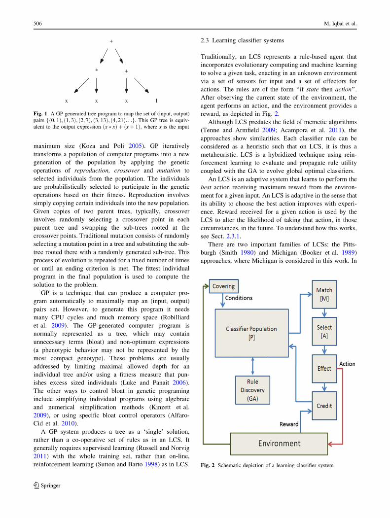
Traditionally, an LCS represents a rule-based agent that

incorporates evolutionary computing and machine learning

to solve a given task, enacting in an unknown environment

via a set of sensors for input and a set of effectors for

actions. The rules are of the form ‘‘if state then action’’.

After observing the current state of the environment, the

agent performs an action, and the environment provides a

reward, as depicted in Fig. 2.

Although LCS predates the field of memetic algorithms

(Tenne and Armfield 2009; Acampora et al. 2011), the

approaches show similarities. Each classifier rule can be

considered as a heuristic such that on LCS, it is thus a

metaheuristic. LCS is a hybridized technique using rein-

forcement learning to evaluate and propagate rule utility

coupled with the GA to evolve global optimal classifiers.

An LCS is an adaptive system that learns to perform the

best action receiving maximum reward from the environ-

ment for a given input. An LCS is adaptive in the sense that

its ability to choose the best action improves with experi-

ence. Reward received for a given action is used by the

LCS to alter the likelihood of taking that action, in those

circumstances, in the future. To understand how this works,

see Sect. 2.3.1.

There are two important families of LCSs: the Pitts-

burgh (Smith 1980) and Michigan (Booker et al. 1989)

approaches, where Michigan is considered in this work. In

*

x x x 1

+

+

Fig. 1 A GP generated tree program to map the set of (input, output)

pairs fð0; 1Þ; ð1; 3Þ; ð2; 7Þ; ð3; 13Þ; ð4; 21Þ. . .g: This GP tree is equiv-

alent to the output expression ðx � xÞ þ ðxþ 1Þ; where x is the input

Fig. 2 Schematic depiction of a learning classifier system

506 M. Iqbal et al.

123

a Michigan-style LCS, population consists of a single set of

co-operative rules, i.e. each individual represents a unique,

distinct rule. The goal here is to find the best set of clas-

sifier rules that, when applied, gain an optimum result for

the problem to be solved. Michigan-style LCSs have two

main types of fitness definitions: strength-based, e.g. ZCS

(Wilson 1994) and accuracy-based, e.g. XCS (Wilson

1995), where the latter is adopted here as it provides a

complete mapping of states to reward.

LCS can be applied to a wide range of problems (Lanzi

et al. 2000) including reinforcement learning problems,

classification problems and function approximation (Butz

2007). LCS have also been adapted to supervised learning

where the environment also returns the ‘correct’ optimal

action through the UCS (sUpervised Classifier System)

framework (Orriols-Puig and Bernado-Mansilla 2006).

UCS is an accuracy-based LCS, specifically designed for

supervised learning problems. In XCS, fitness is computed

using a reinforcement learning scheme so it provides a

complete mapping of states to reward, whereas in UCS

fitness is calculated from a supervised learning perspective

so it evolves a best action map (Bernad-Mansilla and

Garrell-Guiu 2003). UCS can only be applied to single-step

classification tasks, where supervision is available. How-

ever, XCS is more general and can be applied to multi-step

problems and online environments, i.e. interacting with the

environment and obtaining reward according to the per-

formed action.

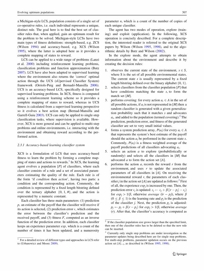
2.3.1 Accuracy-based learning classifier system

XCS is a formulation of LCS that uses accuracy-based

fitness to learn the problem by forming a complete map-

ping of states and actions to rewards.1 In XCS, the learning

agent evolves a population [P] of classifiers, where each

classifier consists of a rule and a set of associated param-

eters estimating the quality of the rule. Each rule is of

the form ‘if condition then action’, having two parts: a

condition and the corresponding action. Commonly, the

condition is represented by a fixed length bitstring defined

over the ternary alphabet {0, 1, #}, and the action is

represented by a numeric constant.

Each classifier has three main parameters: (1) prediction

p, an estimate of the payoff that the classifier will receive if

its action is selected, (2) prediction error �; which estimates

the error between the classifier’s prediction and the

received payoff, and (3) fitness F, computed as an inverse

function of the prediction error. In addition, each classifier

keeps an experience parameter exp, which is a count of the

number of times it has been updated, and a numerosity

parameter n, which is a count of the number of copies of

each unique classifier.

The agent has two modes of operation, explore (train-

ing) and exploit (application). In the following, XCS

operation is concisely described. For a complete descrip-

tion, the interested reader is referred to the original XCS

papers by Wilson (Wilson 1995, 1998), and to the algo-

rithmic details by Butz and Wilson (2002).

In the explore mode, the agent attempts to obtain

information about the environment and describe it by

creating the decision rules:

1. observes the current state of the environment, s 2 S;

where S is the set of all possible environmental states.

The current state s is usually represented by a fixed

length bitstring defined over the binary alphabet {0, 1}.

2. selects classifiers from the classifier population [P] that

have conditions matching the state s, to form the

match set [M].

3. performs covering: for every action ai 2 A in the set of

all possible actions, if ai is not represented in [M] then a

random classifier is generated with a given generaliza-

tion probability such that it matches s and advocates

ai, and added to the population (termed covering).2 The

prediction, prediction error, and fitness of the generated

classifier are set to very small initial values.

4. forms a system prediction array, P(ai) for every ai 2 A

that represents the system’s best estimate of the payoff

should the action ai be performed in the current state s.

Commonly, P(ai) is a fitness weighted average of the

payoff predictions of all classifiers advocating ai.

5. selects an action a to explore (probabilistically or

randomly) and selects all the classifiers in [M] that

advocated a to form the action set [A].

6. performs the action a, records the reward r from the

environment, and uses r to update the associated

parameters of all classifiers in [A]. On receiving the

environmental reward r, the parameters of each clas-

sifier j in the action set [A] are updated as follows:3 First

of all, the experience expj is increased by one. Then, the

prediction error �j is updated: �j �j þ bðjr � pjj � �jÞfor expj [ 1/b, otherwise average (|r - pj|), where b(0 B b B 1) is the learning rate and pj is the prediction

of the classifier j. Next, the prediction pj is adjusted:

pj pj þ bðr � pjÞ for expj [ 1/b, otherwise average

(r). After that, the classifier’s accuracy is computed as

1 For a detailed review of different types and approaches in LCS refer

to (Urbanowicz and Moore 2009).

2 If the classifier population size grows larger than the specified limit,

then one of the classifier rules has to be deleted so that the new rule

can be inserted.3 Currently only single step problems are under investigation so the

parameter updates being described here are for single step problems.

For multi-step problems, parameter updation occurs on the previous

action set [A]-1, as described in (Wilson 1995, 1998).


123

an inverse function of the classifier’s error: kj ¼að�j=�0Þ�m

for �j� �0; otherwise 1. The parameter

�0ð�0 [ 0Þ determines the threshold error under which a

classifier is considered to be accurate, providing

robustness to noise. The parameters a (0 \ a\ 1)

and m (m[ 0) control the degree of decline in accuracy

if the classifier is inaccurate (Butz et al. 2001). The

parameter m separates rules of similar fitness to increase

the probability for selection of better rules. Then,

the relative accuracy k0j is computed by dividing the

accuracy kj by the total amount of accuracies in the

action set. Finally, the fitness Fj is updated according to

the classifier’s relative accuracy: Fj Fj þ bðk0j � FjÞ:Note that basing fitness on the relative accuracies

provides fitness sharing among the classifiers belonging

to the same action set. Fitness sharing allocates

resources to niches evenly, i.e. unbalanced classes or

complex classes do not get ignored.

7. when appropriate, implements rule discovery by

applying an evolutionary mechanism (commonly a

GA) in the action set [A], to introduce new classifiers

to the population. First of all, two parent classifiers are

selected from [A] based on fitness and the offspring are

created out of them. Next, the conditions of the

offspring are crossed with probability v and then each

bit in the conditions is mutated with probability l such

that both offspring match the currently observed state

s. After that, the actions of the produced offspring are

mutated with probability l.

The experience and numerosity of the offspring are set

to 0 and 1, respectively. If the offspring are crossed and/

or mutated then their prediction is set to the average of

the parents’ values. The prediction error and fitness of

the crossed and/or mutated offspring are set to the

average of the parents’ values reduced by constants pre-

dictionErrorReduction and fitnessReduction, respec-

tively (Butz 2000). It is to be noted that in XCS, only

two children are produced by evolutionary operation, as

opposed to typical GA and GP evolution where the

whole population is replaced by the newly generated

individuals. In XCS, the genetic operations are applied

in sequence on two selected parent classifiers to

produce two offspring, whereas in the GA and GP the

genetic operations are applied in parallel on the whole

population of individuals to produce the new genera-

tion of individuals that replace all the current gener-

ation. The XCS rule discovery operation is illustrated

graphically with an example in Sect. 3.

Additionally, the explore mode may perform subsump-

tion, to merge specific classifiers into any more general and

accurate classifiers. If an offspring generated by the GA has

the same action as that of the parents, then its parents are

examined to see if either of them: (1) has an experience

value greater than a threshold, (2) is accurate, and (3) the

environmental inputs it matches are a superset of the inputs

matched by the offspring. If this test is satisfied, the off-

spring is discarded and the numerosity of the parent is

incremented by one. A similar check for subsumption can

be done in action sets to subsume any less general classi-

fiers in an action set [A] by the most general subsumer

classifier in the set [A]. Subsumption deletion is a way of

biasing the genetic search towards more general, but still

accurate, classifiers (Wilson 1998). It also effectively

reduces the number of classifier rules in the final popula-

tion (Kovacs 1996).

In contrast to the explore mode, in the exploit mode the

agent does not attempt to discover new information and

simply performs the action with the best predicted payoff.

The exploit mode is also used to test learning performance

of the agent in the application.

The generalization property in LCS allows a single rule to

cover more than one state provided that the action-reward

mapping is similar. Traditionally, generalization in LCS

classifier conditions is achieved by the use of a special ‘don’t

care’ symbol (#) in the ternary representation, which matches

any value of a specified attribute in the vector describing the

state s. The next section presents various other representa-

tions that have been successfully used in XCS.

2.3.2 XCS’s variations

Various richer encoding schemes have been investigated in

the LCS research community in an attempt to improve the

generalization, to obtain compact classifier rules, to reach the

optimal performance faster, and to investigate scalability of

the learning system. Most of these schemes have been

implemented on Wilson’s XCS, which is the most tested and

the best performing model of learning classifier systems.

In 1999, Lanzi experimented with two different ways to

represent classifier conditions: firstly the fixed-length bit-

strings coding of classifier conditions was replaced with a

variable-length messy coding (Lanzi 1999) in which

environmental inputs were translated into the bitstrings that

have no positional linking between the bits in classifier

condition and any feature in the environmental input. Then,

he extended a step further from messy coding to a more

complex representation in which S-expressions were used

to represent general classifier conditions (Lanzi and

Perrucci 1999).4

In 2002, Wilson introduced the idea of computed pre-

diction, as a function of classifier condition and a weight

4 S-expressions are list-based data structures that are suitable for

representing arbitrary complex data. An S-expression is defined

recursively as either a byte-string or a list of simpler S-expression. For

a more detailed description of S-expressions refer to (Rivest 1997).

508 M. Iqbal et al.

123

vector, to learn approximations to functions (Wilson 2002).

The classifier condition was changed from ternary alphabet

string to a concatenation of interval-based numeric values.

The implemented system is known as XCSF in the LCS

research community. Lanzi et al. (2005) used XCSF for the

learning of Boolean functions. They have shown that

XCSF can produce more compact classifier rules as com-

pared to XCS, since the use of computed prediction allows

more general solutions (Lanzi et al. 2007).

In 2006, Butz et al. incorporated the EDA mechanism in

XCS to identify and process building blocks for solving

hierarchical decomposable binary classification problems

(Butz et al. 2006). They have used extended compact GA

(ECGA) and the Bayesian optimization algorithm (BOA) to

estimate the probability of distribution. In domains con-

taining building blocks, this approach has shown the benefits

of not using the potentially destructive crossover operation.

In 2007, Charalambos and Browne investigated scaling

of an abstract LCS using pre-constructed functions for a

specific problem domain (Ioannides and Browne 2007).

They implemented classifier conditions as a combination of

ternary and S-expression alphabets. They have shown that

using domain-relevant functions the scalability of XCS can

be improved. However, without domain knowledge the

appropriate functions for a problem need to be automati-

cally discovered.

In July 2007, Lanzi and Loiacono (2007) introduced a

version of XCS with computed actions, named XCSCA, to

be used for problem domains involving a large number of

actions. The classifier action was computed using a

parametrized function in a supervised fashion. They have

shown that XCSCA can evolve accurate and compact

representations of binary functions which would be diffi-

cult to solve using a typical XCS model. Then in Sep-

tember 2007, they extended XCSCA using support vector

machines to compute the classifier action (Loiacono et al.

2007). This extension resulted in reaching optimal perfor-

mance faster than XCSCA.

A GP-based rich encoding has been used by Ahluwalia

et al. (Ahluwalia and Bull 1999) within a simplified

strength-based learning classifier system (Wilson 1994).

They used binary strings to represent condition and an

S-expression to represent the action of a classifier rule. This

GP-based LCS generates filters for feature extraction,

rather than performing classification directly. The extracted

features are used by the K-Nearest Neighbour algorithm to

perform classification.

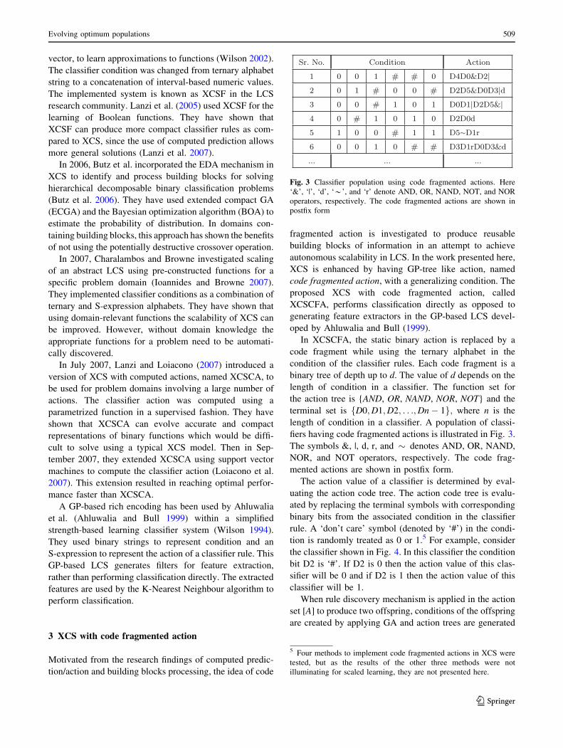
3 XCS with code fragmented action

Motivated from the research findings of computed predic-

tion/action and building blocks processing, the idea of code

fragmented action is investigated to produce reusable

building blocks of information in an attempt to achieve

autonomous scalability in LCS. In the work presented here,

XCS is enhanced by having GP-tree like action, named

code fragmented action, with a generalizing condition. The

proposed XCS with code fragmented action, called

XCSCFA, performs classification directly as opposed to

generating feature extractors in the GP-based LCS devel-

oped by Ahluwalia and Bull (1999).

In XCSCFA, the static binary action is replaced by a

code fragment while using the ternary alphabet in the

condition of the classifier rules. Each code fragment is a

binary tree of depth up to d. The value of d depends on the

length of condition in a classifier. The function set for

the action tree is {AND, OR, NAND, NOR, NOT} and the

terminal set is fD0;D1;D2; . . .;Dn� 1g; where n is the

length of condition in a classifier. A population of classi-

fiers having code fragmented actions is illustrated in Fig. 3.

The symbols &, |, d, r, and � denotes AND, OR, NAND,

NOR, and NOT operators, respectively. The code frag-

mented actions are shown in postfix form.

The action value of a classifier is determined by eval-

uating the action code tree. The action code tree is evalu-

ated by replacing the terminal symbols with corresponding

binary bits from the associated condition in the classifier

rule. A ‘don’t care’ symbol (denoted by ‘#’) in the condi-

tion is randomly treated as 0 or 1.5 For example, consider

the classifier shown in Fig. 4. In this classifier the condition

bit D2 is ‘#’. If D2 is 0 then the action value of this clas-

sifier will be 0 and if D2 is 1 then the action value of this

classifier will be 1.

When rule discovery mechanism is applied in the action

set [A] to produce two offspring, conditions of the offspring

are created by applying GA and action trees are generated

Fig. 3 Classifier population using code fragmented actions. Here

‘&’, ‘|’, ‘d’, ‘*’, and ‘r’ denote AND, OR, NAND, NOT, and NOR

operators, respectively. The code fragmented actions are shown in

postfix form

5 Four methods to implement code fragmented actions in XCS were

tested, but as the results of the other three methods were not

illuminating for scaled learning, they are not presented here.


123

by applying GP-based genetic operations. First of all, two

parent classifiers are selected from [A] based on fitness and

the offspring are created out of them. Next, the conditions

and action trees of the offspring are crossed with proba-

bility v by applying GA and GP crossover operations,

respectively. After that, the conditions of the resulted

children by crossover are mutated with probability l, such

that both children match the currently observed state

s. Then, the action trees of the children are mutated with

probability pm, to replace a subtree of the action with a

randomly generated subtree of depth up to 1.

For example, consider the rule discovery operation

graphically summarized in Fig. 5. Figure 5a shows the

action set containing three classifiers with action value 1,

formed from the classifier population [P] shown in Fig. 3,

against the environmental input s = 001010. First of all,

two parent classifiers are selected, Fig. 5b, from the action

set based on fitness F, and two children are created out of

them, Fig. 5c. Then, in Fig. 5d, the conditions of the

reproduced children are crossed over by applying two-point

GA-crossover operation at the two marked points, and the

action trees of the children are crossed over by applying

GP-crossover operation. The fitness value of crossed over

children is set to the average of parents’ fitness values

reduced by 0.1, as suggested by Butz et al. in (Butz and

Wilson 2002). After that, Fig. 5e, the conditions of the

crossed over children are mutated by applying GA-mutation

such that both children match the currently observed state

s = 001010, and the action trees of the children are mutated

by applying GP-mutation. The final children generated in the

rule discovery operation are shown in Fig. 5f.

It is to be noted that the advantages of subsumption

deletion are lost due to genotypic differences resulting in

subsumption not occurring despite phenotypically similar

behaviour. Subsumption deletion is made possible, albeit

still problematic, by matching the action code on a

character by character base. To avoid volatility in per-

formance of the system due to the issue of inconsistency

of a classifier’s action value (to be discussed in

Sect. 6.2), it is necessary for the subsumer to have

consistent action value, in addition to being accurate and

experienced.

If a newly created classifier in the rule discovery oper-

ation is not subsumed by the parents and there is no clas-

sifier equal to it in the population, then it will be added to

the population. Two classifiers are considered to be equal,

if and only if both have the same condition and the same

code fragmented action tree.

Fig. 4 A classifier rule with code fragmented action. Here ‘|’ and ‘&’

denote logical OR and logical AND operators, respectively

(a)

(b)

(c)

(d)

(e)

(f)

Fig. 5 Rule discovery by applying GA and GP operations in the

action set [A] formed from the classifier population [P] shown in

Fig. 3, against the environmental input s = 001010. a action set

containing three classifiers with action value 1, b two parent

classifiers selected from the action set based on fitness F, c two

reproduced children, d crossed over children produced by applying

two-point GA-crossover on the conditions and GP-crossover on the

action trees of the reproduced offspring classifiers, with fitness values

equal to average of parents’ fitness values reduced by 0.1, e mutated

children produced by applying GA-mutation on the conditions and

GP-mutation on the action trees of the crossed over offspring

classifiers, and f final children generated in the rule discovery

operation

510 M. Iqbal et al.

123

4 The problem domain and experimental setup

The problem domain used in the experimentation is the

multiplexer problem, which is commonly used by the LCS

research community. Multiplexer problems are considered

to be interesting because they are highly non-linear and,

therefore, relatively difficult to learn. They also allow

generalizations and are suitable for examining the scala-

bility of the algorithm.

4.1 Multiplexer problem domain

A multiplexer is an electronic circuit that accepts n input

signals and gives one output signal. The n inputs are

divided into two groups: k address bits and the remaining

n-k data bits. Actually n is of the form k ? 2k. Hence the

data bits are n - k = 2k. For n input signals, there can be

2n different input combinations. The values of address bits

are used to select the data bit to be given as output. In 6-bits

multiplexer problem, there are two address bits and four

data bits. If we denote the address bits by A0 and A1 and

the data bits by D0, D1, D2, and D3 then the four cases for

6-bits multiplexer to decide its output signal are

• if A1 = 0 and A0 = 0 then the output is the value of data

bit D0,


bit D1,


bit D2, and


bit D3.

For example, if the input is 011101 then the output will

be 1 and if the input is 101101 then the output will be 0.6

Because in the multiplexer problem domain output

signal depends upon the address bits, the set of input

combinations can be generalized. For example in the case

of 6-bits multiplexer problem, the output for inputs

100101, 101100, and 101001 is 0 because in all these three

input combinations, the output is the value of the data bit

D2 and we do not care about the values of other data bits. If

we use ‘# as the ‘don’t care’ symbol (it can be either 0 or 1)

then these three input instances can be generalized as

10##0#.7 The complete generalized set of inputs along with

the accurate outputs, for 6-bits multiplexer, is shown in

Table 1.

In the experimentation, both address and data bits are

denoted by D (instead of denoting address bits by A and

data bits by D), as the LCS has no domain knowledge

on the purpose of the bits and the ordering of bits is

irrelevant to the learning system provided it is consistent.

As is common practice, the environment has left most

bits for the address and the remaining bits for the data,

e.g. in case of 6-bits multiplexer D0 and D1 represent

address bits and the remaining D2 to D5 represent data

bits.

4.2 Experimental setup

The system uses the following, commonly used in the

literature, parameter values as suggested by Butz and

Wilson (2002) and Butz (2000): fitness fall-off rate

a = 0.1; prediction error threshold �0 ¼ 10; fitness expo-

nent m = 5; learning rate b = 0.2; threshold for GA

application in the action set hGA = 25; experience

threshold for classifier deletion hdel = 20; fraction of

mean fitness for deletion d = 0.1; classifier experience

threshold for subsumption hsub = 20; crossover probabil-

ity v = 0.8; condition mutation probability l = 0.04;

action mutation probability pm = 0.1; initial prediction

pI = 10.0; initial prediction error �I ¼ 0:0; initial fitness

FI = 0.01; reduction of the prediction error prediction-

ErrorReduction = 0.25; reduction of the fitness fitness-

Reduction = 0.1; maximum allowed tree depth d is set to

2 for 6-bits and 11-bits multiplexer problems whereas to 3

for 20-bits and 37-bits multiplexer problems; and the

selection method is tournament selection with tournament

size ratio 0.4. Probability of ‘#’ in covering is set to 0.5

for 6-, 11-, and 20-bits multiplexers whereas to 0.75 for

37-bits multiplexer. The number of micro classifiers used

is 500, 1,000, 2,000, and 8,000 for 6-, 11-, 20-, and

37-bits multiplexers, respectively. Explore and exploit

problems are alternated with probability 0.5. All the

experiments have been repeated 30 times with a known

different seed in each run. One run is stopped after one

million explore problems.

Table 1 Optimum ternary encoded rule set for the 6-bits multiplexer

problem

Input Output

A1 A0 D0 D1 D2 D3

0 0 0 # # # 0

0 0 1 # # # 1

0 1 # 0 # # 0

0 1 # 1 # # 1

1 0 # # 0 # 0

1 0 # # 1 # 1

1 1 # # # 0 0

1 1 # # # 1 1

6 It is assumed that the order of bits is A1A0D0D1D2D3.7 The generalized input 10##0# actually covers eight input combi-

nations: 100000, 100001, 100100, 100101, 101000, 101001, 101100,

and 101101.


123

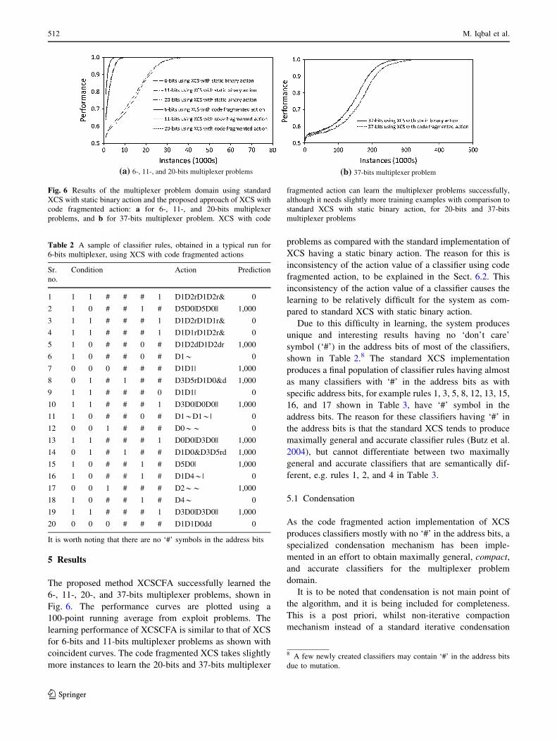
5 Results

The proposed method XCSCFA successfully learned the

6-, 11-, 20-, and 37-bits multiplexer problems, shown in

Fig. 6. The performance curves are plotted using a

100-point running average from exploit problems. The

learning performance of XCSCFA is similar to that of XCS

for 6-bits and 11-bits multiplexer problems as shown with

coincident curves. The code fragmented XCS takes slightly

more instances to learn the 20-bits and 37-bits multiplexer

problems as compared with the standard implementation of

XCS having a static binary action. The reason for this is

inconsistency of the action value of a classifier using code

fragmented action, to be explained in the Sect. 6.2. This

inconsistency of the action value of a classifier causes the

learning to be relatively difficult for the system as com-

pared to standard XCS with static binary action.

Due to this difficulty in learning, the system produces

unique and interesting results having no ‘don’t care’

symbol (‘#’) in the address bits of most of the classifiers,

shown in Table 2.8 The standard XCS implementation

produces a final population of classifier rules having almost

as many classifiers with ‘#’ in the address bits as with

specific address bits, for example rules 1, 3, 5, 8, 12, 13, 15,

16, and 17 shown in Table 3, have ‘#’ symbol in the

address bits. The reason for these classifiers having ‘#’ in

the address bits is that the standard XCS tends to produce

maximally general and accurate classifier rules (Butz et al.

2004), but cannot differentiate between two maximally

general and accurate classifiers that are semantically dif-

ferent, e.g. rules 1, 2, and 4 in Table 3.

5.1 Condensation

As the code fragmented action implementation of XCS

produces classifiers mostly with no ‘#’ in the address bits, a

specialized condensation mechanism has been imple-

mented in an effort to obtain maximally general, compact,

and accurate classifiers for the multiplexer problem

domain.

It is to be noted that condensation is not main point of

the algorithm, and it is being included for completeness.

This is a post priori, whilst non-iterative compaction

mechanism instead of a standard iterative condensation

(a) 6-, 11-, and 20-bits multiplexer problems (b) 37-bits multiplexer problem

Fig. 6 Results of the multiplexer problem domain using standard

XCS with static binary action and the proposed approach of XCS with

code fragmented action: a for 6-, 11-, and 20-bits multiplexer

problems, and b for 37-bits multiplexer problem. XCS with code

fragmented action can learn the multiplexer problems successfully,

although it needs slightly more training examples with comparison to

standard XCS with static binary action, for 20-bits and 37-bits

multiplexer problems

Table 2 A sample of classifier rules, obtained in a typical run for

6-bits multiplexer, using XCS with code fragmented actions

Sr.

no.

Condition Action Prediction

1 1 1 # # # 1 D1D2rD1D2r& 0

2 1 0 # # 1 # D5D0|D5D0|| 1,000

3 1 1 # # # 1 D1D2rD1D1r& 0

4 1 1 # # # 1 D1D1rD1D2r& 0

5 1 0 # # 0 # D1D2dD1D2dr 1,000

6 1 0 # # 0 # D1* 0

7 0 0 0 # # # D1D1| 1,000

8 0 1 # 1 # # D3D5rD1D0&d 1,000

9 1 1 # # # 0 D1D1| 0

10 1 1 # # # 1 D3D0|D0D0|| 1,000

11 1 0 # # 0 # D1*D1*| 0

12 0 0 1 # # # D0** 0

13 1 1 # # # 1 D0D0|D3D0|| 1,000

14 0 1 # 1 # # D1D0&D3D5rd 1,000

15 1 0 # # 1 # D5D0| 1,000

16 1 0 # # 1 # D1D4*| 0

17 0 0 1 # # # D2** 1,000

18 1 0 # # 1 # D4* 0

19 1 1 # # # 1 D3D0|D3D0|| 1,000

20 0 0 0 # # # D1D1D0dd 0

It is worth noting that there are no ‘#’ symbols in the address bits

8 A few newly created classifiers may contain ‘#’ in the address bits

due to mutation.

512 M. Iqbal et al.

123

technique. In a typical condensation method (Wilson 1995;

Kovacs 1996), evolutionary search is suspended by stop-

ping the GA creating new classifiers and learning continues

for a certain number of iterations. In the condensation

mechanism being introduced here, training is stopped and

the rule set is compacted instantly.

The specialized condensation algorithm for this imple-

mentation is given below:

1. From the final rule set, delete all the classifiers that are

either inaccurate (i.e., prediction error �[ �0), or less

experienced (i.e., experience exp B 1/b), or have

inconsistent action values.

2. In the remaining population, if two classifiers have the

same condition, the same action value, and the same

prediction value, then treat them as a single classifier.

Delete one of them and increase the numerosity of the

other by the numerosity value of the one being deleted.

The classifier being kept retains the higher experience

and fitness values from these two classifiers.

3. In the resulting population of step 2, if two classifiers

have the same condition, but opposite action (i.e. 0/1)

and likewise the opposite prediction values (i.e.

0/1,000), then invert the action and prediction values

of the classifier having prediction value equal to 0 and

condense them as a single classifier. Delete one of

(a) 6-bits multiplexer (b) 11-bits multiplexer

(c) 20-bits multiplexer (d) 37-bits multiplexer

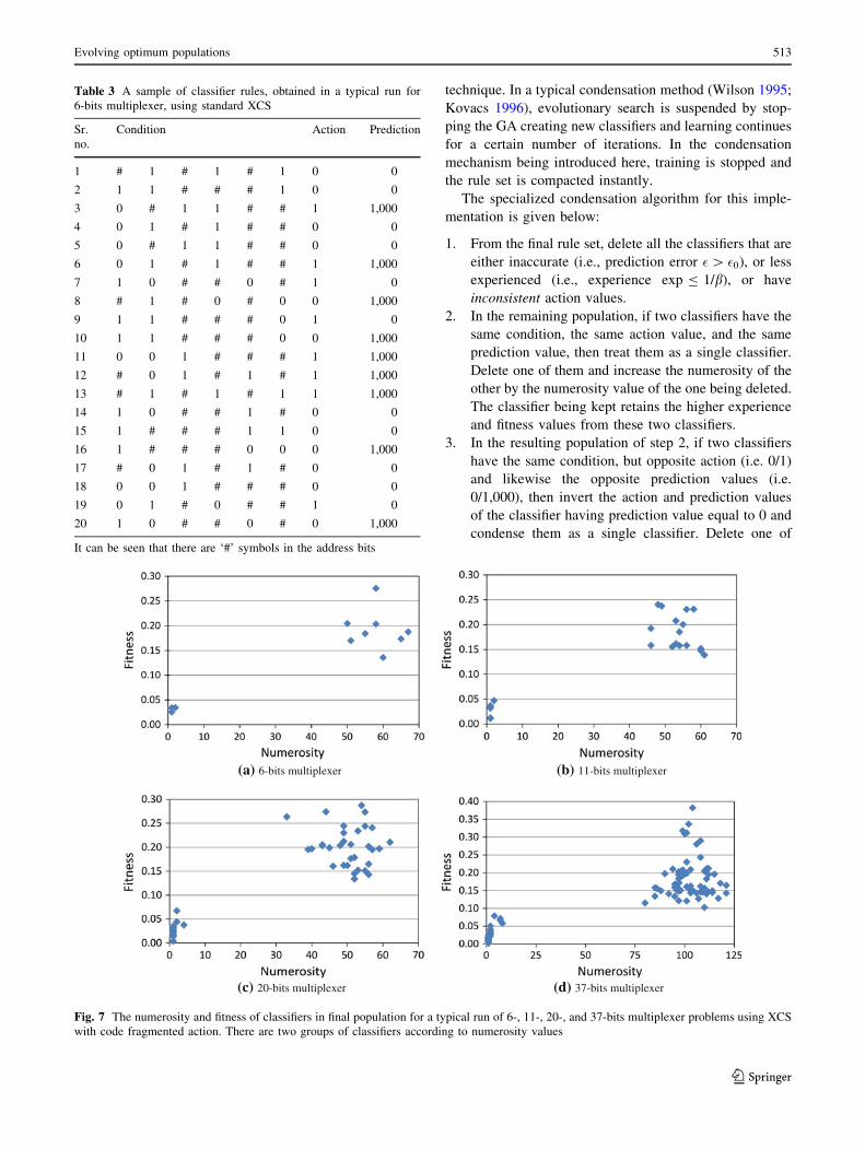
Fig. 7 The numerosity and fitness of classifiers in final population for a typical run of 6-, 11-, 20-, and 37-bits multiplexer problems using XCS

with code fragmented action. There are two groups of classifiers according to numerosity values

Table 3 A sample of classifier rules, obtained in a typical run for

6-bits multiplexer, using standard XCS

Sr.

no.

Condition Action Prediction

1 # 1 # 1 # 1 0 0

2 1 1 # # # 1 0 0

3 0 # 1 1 # # 1 1,000

4 0 1 # 1 # # 0 0

5 0 # 1 1 # # 0 0

6 0 1 # 1 # # 1 1,000

7 1 0 # # 0 # 1 0

8 # 1 # 0 # 0 0 1,000

9 1 1 # # # 0 1 0

10 1 1 # # # 0 0 1,000

11 0 0 1 # # # 1 1,000

12 # 0 1 # 1 # 1 1,000

13 # 1 # 1 # 1 1 1,000

14 1 0 # # 1 # 0 0

15 1 # # # 1 1 0 0

16 1 # # # 0 0 0 1,000

17 # 0 1 # 1 # 0 0

18 0 0 1 # # # 0 0

19 0 1 # 0 # # 1 0

20 1 0 # # 0 # 0 1,000

It can be seen that there are ‘#’ symbols in the address bits


123

them and increase the numerosity of the other by the

numerosity value of the one being deleted. The

classifier being kept retains the higher experience

and fitness values from these two classifiers.9

4. Sort the resulting population of step 3 according to

numerosity in descending order.

5. Find the two consecutive classifiers that have the

maximum numerosity difference between each other:

say they are C1 and C2 such that numerosity of

classifier C1 is greater than that of C2.

6. Delete all the classifiers having numerosity equal to or

less than the numerosity of C2.

When applying steps 1–4 of the condensation mecha-

nism, the population of classifiers automatically separated

into two groups according to numerosity values. Figure 7

shows the separation of classifiers, for a typical run of

6-, 11-, 20-, and 37-bits multiplexer problems. It can be seen

that the group of classifiers having higher numerosity values

also have higher fitness values as would be expected. So the

classifiers with low numerosity were deleted, applying steps

5–6 of the condensation algorithm, to obtain a final popu-

lation of maximally general, compact, and accurate classi-

fiers. The resulting population has 8, 16, 32, and 64

classifiers for 6-, 11-, 20-, and 37-bits multiplexer problems,

respectively. The final populations for 6-bits and 11-bits

multiplexers are shown in Tables 4 and 5, respectively.

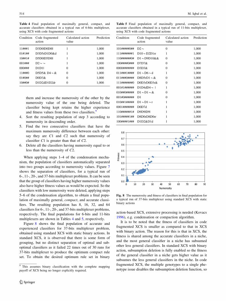
Figure 8 shows the final population of accurate and

experienced classifiers for 37-bits multiplexer problem,

obtained using standard XCS with static binary actions. In

standard XCS, it is observed that there is some form of

grouping, but no distinct separation of optimal and sub-

optimal classifiers as it failed 22 times out of 30 runs for

37-bits multiplexer to produce the optimum compact rule

set. To obtain the desired optimum rule set in binary

action-based XCS, extensive processing is needed (Kovacs

1996), e.g. condensation or compaction algorithm.

It is to be noted that the fitness of classifiers in code

fragmented XCS is smaller as compared to that in XCS

with binary action. The reason for this is that in XCS, the

fitness is shared among the accurate classifiers in a niche,

and the most general classifier in a niche has subsumed

other less general classifiers. In standard XCS with binary

action, subsumption deletion is fully enabled so the fitness

of the general classifier in a niche gets higher value as it

subsumes the less general classifiers in the niche. In code

fragmented XCS, the multiple genotypes to a single phe-

notype issue disables the subsumption deletion function, so

Table 4 Final population of maximally general, compact, and

accurate classifiers obtained in a typical run of 6-bits multiplexer,

using XCS with code fragmented actions

Condition Code fragmented

action

Calculated action

value

Prediction

11###1 D3D0|D0D0|| 1 1,000

01#1## D3D5rD1D0&d 1 1,000

10##1# D5D0|D5D0|| 1 1,000

001### D2** 1 1,000

000### D1D1| 0 1,000

11###0 D5D5& D4*& 0 1,000

01#0## D0D3& 0 1,000

10##0# D1D2dD1D2dr 0 1,000

Table 5 Final population of maximally general, compact, and

accurate classifiers obtained in a typical run of 11-bits multiplexer,

using XCS with code fragmented actions

Condition Code fragmented

action

Calculated action

value

Prediction

101#####0## D2* 0 1,000

111#######1 D10*D2D1rr 1 1,000

110######0# D1*D9D10&& 0 1,000

100####0### D7D7& 0 1,000

0000####### D3D3& 0 1,000

011###1#### D1*D6*d 1 1,000

011###0#### D8D5rD1*& 0 1,000

111#######0 D0D3rD0D3r& 0 1,000

001#1###### D1D4dD4* | 1 1,000

010##0##### D1*D1*& 0 1,000

001#0###### D1 0 1,000

010##1##### D1*D1*r 1 1,000

0001####### D0D7d 1 1,000

110######1# D9D9|D9| 1 1,000

101#####1## D8D0rD8D0rr 1 1,000

100####1### D1D2&D1d 1 1,000

Fig. 8 The numerosity and fitness of classifiers in final population for

a typical run of 37-bits multiplexer using standard XCS with static

binary actions

9 This assumes binary classification with the complete mapping

payoff of XCS being no longer explicitly required.

514 M. Iqbal et al.

123

fitness in a niche is distributed among multiple equally

general classifiers, all having a relatively small fitness

value as compared to the binary action-based XCS.

6 Discussions

It was not the primary goal to produce a maximally gen-

eral, accurate and compact population. The main aim of

this experimentation was to investigate the scalability of

building blocks within LCS, but it resulted in the seren-

dipity of producing the optimum solution. The following

sections elaborate why the optimum solution was

produced.

6.1 Specialization of address bits

If there are no ‘#’ bits in the address bits then the system

requires just one specific data bit, at the correct position, to

generate an accurate rule. If there is a ‘#’ symbol in the

address bits then it needs at least two specific data bits, at

the correct positions and having the same value, to produce

an accurate rule (which will actually cover two simple

rules). For example, in Table 6 there is no ‘#’s in the

address bits for first two rules so just one specific data bit is

enough to make them accurate classifiers whereas the third

rule has a ‘#’ in address bits so it needs two specific data

bits to be accurate. Similarly the fourth rule, having two

‘don’t care’ symbols in the address bits, needs four specific

data bits to be an accurate rule. It is to be noted that the

correctness of the rules depend on the value of action, e.g.,

in the case of these four rules, if action value is ‘1’ then

they will be correct, otherwise they are incorrect classifiers.

Each ‘don’t care’ symbol in the address bits makes it

difficult for the system to produce an accurate classifier

rule, although if it is produced then it will cover more than

one classifier so the final population of classifiers would

have relatively fewer classifiers than enumerated specific

classifiers. If there are n ‘don’t care’ symbols in the address

bits of a classifier then the system needs at least 2n specific

data bits, at correct positions with the same value, in the

classifier to make it an accurate classifier rule. If it is

produced, it will be equivalent to 2n simpler classifiers.

If the action is binary (as in standard XCS implemen-

tation) then it is relatively easy for the system to produce

such classifier rules. However, in our case, the action is a

code fragment and the action value is determined by taking

the associated condition as its input where ‘#’ in the con-

dition is treated as 0 or 1 randomly. So it heavily depends

on the bits in the associated condition to generate an

accurate action that will result in the accurate classifier

rule. A single ‘#’ symbol in the address bits makes it harder

for this system to produce an accurate corresponding ‘code

fragmented action’ because of inconsistency of action

value. The consistency of a classifier’s action value with

different condition patterns is discussed next.

6.2 Consistency of a classifier’s action value

In the case of standard XCS implementation, all classifier

rules are 100 % consistent in terms of the action value. If a

classifier’s action is 0 then it will be permanently 0 and if it

is 1 then it will be permanently 1 throughout the system

evolution. However in code fragmented action implemen-

tation of XCS, where a classifier’s action value is deter-

mined using the classifier’s condition as input to the code

fragment tree, this is not the case.

In this implementation, the 100 % consistency of the

whole population of classifiers (in terms of action value) is

not guaranteed. The reason of this decreased consistency is

that the ‘#’ symbol in the condition of a classifier is ran-

domly treated as 0 or 1 during the computation of a clas-

sifier’s action value.10

A classifier having no ‘#’ symbol in the condition is

100 % consistent in terms of its action value, but if a clas-

sifier has one or more ‘#’ symbols in the condition then its

consistency depends upon the code fragment tree. If the

value of a code fragment tree is dependent upon a condition

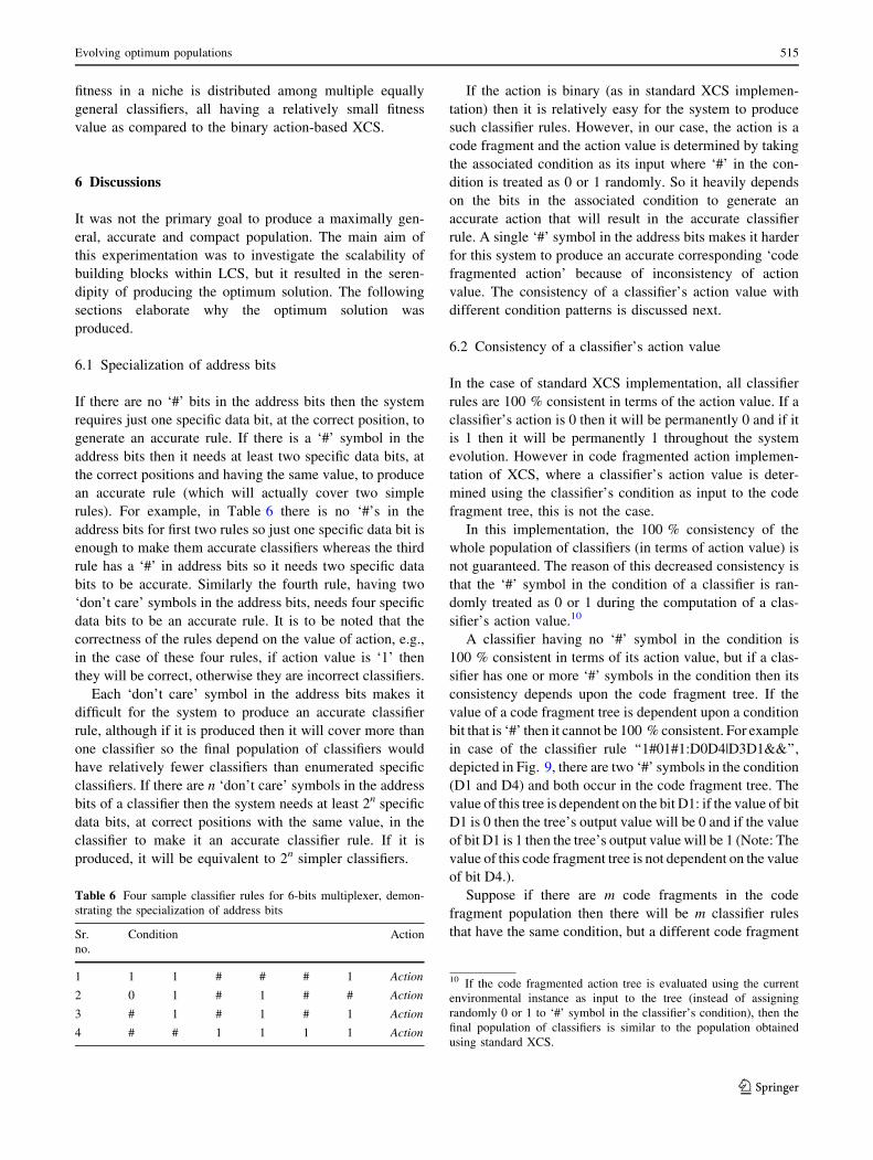
bit that is ‘#’ then it cannot be 100 % consistent. For example

in case of the classifier rule ‘‘1#01#1:D0D4|D3D1&&’’,

depicted in Fig. 9, there are two ‘#’ symbols in the condition

(D1 and D4) and both occur in the code fragment tree. The

value of this tree is dependent on the bit D1: if the value of bit

D1 is 0 then the tree’s output value will be 0 and if the value

of bit D1 is 1 then the tree’s output value will be 1 (Note: The

value of this code fragment tree is not dependent on the value

of bit D4.).

Suppose if there are m code fragments in the code

fragment population then there will be m classifier rules

that have the same condition, but a different code fragment

Table 6 Four sample classifier rules for 6-bits multiplexer, demon-

strating the specialization of address bits

Sr.

no.

Condition Action

1 1 1 # # # 1 Action

2 0 1 # 1 # # Action

3 # 1 # 1 # 1 Action

4 # # 1 1 1 1 Action

10 If the code fragmented action tree is evaluated using the current

environmental instance as input to the tree (instead of assigning

randomly 0 or 1 to ‘#’ symbol in the classifier’s condition), then the

final population of classifiers is similar to the population obtained

using standard XCS.


123

as the action. Some of these classifiers will be 100 %

consistent in terms of their action values and others not.

If a classifier’s action value is consistent (it can be

correct or incorrect)11 then the correct action will lead to a

stable predicted reward of maximum value (1,000 in this

implementation) and similarly the incorrect action will lead

to a stable predicted reward of minimum value (0 in this

implementation). If the action value of a classifier is not

consistent then the predicted reward of the classifier will

never reach the maximum payoff value nor the minimum

payoff value. The predicted reward of a classifier having

inconsistent action value will increase and decrease

depending upon the correctness of its action value for a

given environmental instance of the problem. The incon-

sistency of a classifier in terms of action value results in

inconsistency of the classifier in terms of predicted reward.

A classifier’s accuracy relates to the consistency of its

reward prediction, so a classifier having consistent action

value will be more accurate than a classifier having

inconsistent action value.

6.3 Optimal classifiers

In the case of multiplexer problem domain, the action value

is dependent on the address bits so the code fragments

having specific address bits have a high probability to

survive in the system. If the address bits’ values are spe-

cific, the code fragment will be more consistent in terms of

its value so the classifier will be relatively more accurate

than a classifier having ‘#’ in the address bits. If there is a

‘#’ in the address bits, then the code fragment will be

relatively inconsistent in its value so its accuracy will be

degraded.

To analyze the consistency of action values, consistency

of all address bit patterns in conditions for the 6-bits

multiplexer problem was calculated. There are two address

bits in the 6-bits multiplexer and each of these two bits can

take a value from the ternary alphabet {0, 1, #} so there are

nine (32) different address patterns for 6-bits multiplexer.

Similarly, the four data bits can take values from the ter-

nary alphabet {0, 1, #} so there are 81 (34) different data

patterns for the 6-bits multiplexer. Combining these dif-

ferent address bits and data bits patterns, there are 729 (9

9 81) different conditions. There are six terminals and five

operators of arity {1, 2, 2, 2, 2}, so there are 97,506 dis-

tinct code fragment trees of depth up to two. Using these

729 different conditions and 97506 different code fragment

trees as actions, results in 71,081,874 different classifier

rules. Each of the nine address patterns have 7,897,986

classifiers. The consistency of each of the address patterns

is shown in Table 7. The consistency of each of the four

patterns having both specific address bits is 79.65 %,

whereas the consistency of the last pattern that has ‘#’ in

both of the address bits is just 49.21 %. The patterns with

one specific address bit and one ‘#’ address bit are 64.41 %

consistent in their action values.

Because the classifiers having conditions from the

schema ‘‘AAxxxx’’12 are more consistent in terms of action

values than other classifiers, the former classifiers are more

consistent in terms of reward predictions than the latter

ones. This consistency of reward prediction makes the

classifiers having condition parts from the ‘‘AAxxxx’’

schema more accurate than the other classifiers having

condition parts from the schema ‘‘#Axxxx’’, ‘‘A#xxxx’’,

and ‘‘##xxxx’’. Now in XCS, as the fitness of a classifier

depends on its accuracy of reward prediction, the classifiers

having specific address bits in conditions have higher fit-

ness values than the classifiers having one or more ‘#’

symbols in the address bits.

In XCS, the reproduction is niche based, i.e. a genetic

algorithm (GA) is applied to the classifiers participating in

Table 7 Consistency of classifiers in terms of action values when

using different patterns as the condition

Sr.

no.

Pattern

(condition)

Total

classifiers

Consistent

classifiers

Consistency

percentage

1 00xxxx 7,897,986 6,290,622 79.65

2 01xxxx 7,897,986 6,290,622 79.65

3 10xxxx 7,897,986 6,290,622 79.65

4 11xxxx 7,897,986 6,290,622 79.65

5 0#xxxx 7,897,986 5,087,259 64.41

6 1#xxxx 7,897,986 5,087,259 64.41

7 #0xxxx 7,897,986 5,087,259 64.41

8 #1xxxx 7,897,986 5,087,259 64.41

9 ##xxxx 7,897,986 3,886,488 49.21

Here ‘‘x’’ means 0, 1, or ‘#’

Fig. 9 A classifier rule with code fragmented action where the action

is dependent on a ‘#’ bit in the condition. Here ‘|’ and ‘&’ denote

logical OR and logical AND operators, respectively

11 In the XCS system, accuracy of prediction is more important than

the correctness of the prediction itself.

12 In this schema ‘A’, the address bits, can be either 0 or 1 and ‘x’,

the data bits, can be 0, 1, or ‘#’.

516 M. Iqbal et al.

123

the action set instead of applying it to the whole classifiers

population and according to Wilson (1995):

… within a given action set, the more accurate

classifiers will have higher fitnesses than the less

accurate ones. They will consequently have more

offspring. But by becoming relatively more numer-

ous, those classifiers will gain a larger fraction of the

total relative accuracy (which always equals 1) and so

will have yet more offspring compared to their less

accurate brethren. Eventually, the most accurate

classifiers in the action set will drive out the others, in

principle leaving the X x A ) P map with the best

classifier (assuming the GA has discovered it) for

each situation–action combination.

The classifiers having specific address bits are more

consistent in terms of their action values and also seman-

tically simpler, so they are relatively more accurate clas-

sifiers than other classifiers. Therefore, these simple and

consistent classifiers are preferred by the system. When

condensed using the specifically designed condensation

algorithm, described in Sect. 5.1, these classifiers result in

the maximally general, compact and accurate classifiers in

the final population for multiplexer problem domain, i.e the

optimum population.

7 Conclusions

The learning classifier system implemented using ternary

alphabet-based condition and code fragmented action suc-

cessfully learns the tested multiplexer domain problems,

which is to be expected as LCS have good performance in

this domain. It was unexpected that code fragmented

actions produce an optimal solution, given the GP-like

encoding. Investigations showed that in constructing a

richer alphabet the search space became more difficult,

which produced the optimal solutions.

The consistency of action value is guaranteed in the

standard XCS implementation using static binary actions,

but in the code fragmented action that treats a ‘don’t care’

symbol randomly this consistency of action value cannot

be guaranteed for every classifier. This resulted in a com-

pact solution as classifiers having specific address bits were

more consistent than other potentially correct classifiers

(i.e. correct under sampling assumptions implicit in com-

mon alphabets).

This investigation of code fragments in XCS shows that

the multiple genotypes to a single phenotype issue in fea-

ture rich encodings disables the subsumption deletion

function. The additional methods and increased search

space lead to more training examples being required for

similar levels of performance. This is compensated by the

autonomous separation of optimal and sub-optimal classi-

fiers in the final population, eventually resulting in the

optimum rule set of the maximally general, compact and

accurate classifiers.

The next stage is to introduce a mechanism for treating

two classifiers with the same conditions and consistent

actions outputting the same action values as a single clas-

sifier, during the learning process, in order to fully enable

the subsumption deletion function. Hopefully, this will

result in reducing the number of environmental inputs

required to learn the problem domain.

Ultimately, the identified fit building block units from a

simple problem in a domain (e.g. 6-bit multiplexer) will be

used to seed the population in a more complex problem in

the same problem domain (e.g. 11-bit multiplexer) and so

forth. By utilizing this ‘stepping-stone’ approach it is

hoped that eventually a problem will be solved in the

domain (e.g. 1,034-bit multiplexer), which had not previ-

ously been solved using the base techniques.

It is anticipated that multiple populations of building

block units from different, associated problem domains

will need to be leveraged to assist in general problem

solving.

References

Acampora G, Cadenas JM, Loia V, Ballester EM (2011) A multi-agent

memetic system for human-based knowledge selection. IEEE

Trans Syst Man Cybern A Systems Humans 41(5):946–960

Ahluwalia M, Bull L (1999) A genetic programming based classifier

system. In: Proceedings of the genetic and evolutionary compu-

tation conference, pp 11–18

Alfaro-Cid E, Merelo JJ, de Vega FF, Esparcia-Alcazar AI, Sharman

K (2010) Bloat control operators and diversity in genetic

programming: a comparative study. Evol Comput 18(2):305–332

Altenberg L (1995) The schema theorem and Price’s theorem. In:

Foundations of genetic algorithms, pp 23–49

Banzhaf W, Nordin P, Keller RE, Francone FD (1998) Genetic

programming—an introduction: on the automatic evolution of

computer programs and its applications. Morgan Kaufmann,

Burlington

Bernad-Mansilla E, Garrell-Guiu JM (2003) Accuracy-based learning

classifier systems: models, analysis and applications to classifi-

cation tasks. Evol Comput 11(3):209–238

Beyer HG (1997) An alternative explanation for the manner in which

genetic algorithms operate. BioSystems 41:1–15

Booker LB, Goldberg DE, Holland JH (1989) Classifier systems and

genetic algorithms. Artif Intell 40(1-3):235–282

Burjorjee KM (2008) The fundamental problem with the building

block hypothesis

Butz MV (2000) XCSJava 1.0: an implementation of the XCS

classifier system in Java. Technical Report 2000027, Illinois

Genetic Algorithms Laboratory

Butz MV (2007) Combining gradient-based with evolutionary online

learning: an introduction to learning classifier systems. In:

Proceedings of the seventh international conference on hybrid

intelligent systems, pp 12–17


123

Butz MV, Kovacs T, Lanzi PL, Wilson SW (2001) How XCS evolves

accurate classifiers. Technical Report 2001008, Illinois Genetic

Algorithms Laboratory

Butz MV, Kovacs T, Lanzi PL, Wilson SW (2004) Toward a theory

of generalization and learning in XCS. IEEE Trans Evol Comput

8(1):28–46

Butz MV, Pelikan M, Llora X, Goldberg DE (2006) Automated

global structure extraction for effective local building block

processing in XCS. Evol Comput 14(3):345–380

Butz MV, Wilson SW (2002) An algorithmic description of XCS.

Soft Comput A Fusion Found Methodol Appl 6(3-4):144–153

Drugowitsch J (2008) Design and analysis of learning classifier

systems: a probabilistic approach. Springer Berlin

Eiben AE, Smith JE (2003) Introduction to evolutionary computing,

1st edn. Natural Computing Series. Springer, Berlin

Goldberg DE (1989) Genetic algorithms in search, optimization and

machine learning. Addison Wesley, Boston

Holland JH (1975) Adaptation in natural and artificial systems.

University of Michigan Press, Ann Arbor

Holland JH (1986) Escaping brittleness: the possibilities of general-

purpose learning algorithms applied to parallel rule-based

systems. In: Machine learning: an artificial intelligence

approach, vol II. Morgan Kaufmann, Burlington, pp 593–623

Ioannides C, Browne WN (2007) Investigating scaling of an

abstracted LCS utilising ternary and S-expression alphabets.

In: Proceedings of the genetic and evolutionary computation

conference, pp 2759–2764

Jong KAD (2006) Evolutionary computation: a unified approach. MIT

Press, Cambridge

Kinzett D, Johnston M, Zhang M (2009) Numerical simplification for

bloat control and analysis of building blocks in genetic

programming. Evol Intell 2(4):151–168

Kovacs T (1996) Evolving optimal populations with XCS classifier

systems. Technical Report CSR-96-17 and CSRP-9617, Univer-

sity of Birmingham, UK

Koza JR (1992) Genetic programming: on the programming of

computers by means of natural selection. MIT Press, Cambridge

Koza JR, Poli R (2005) Genetic programming. In: Search method-

ologies: introductory tutorials in optimization and decision

support techniques, chap. 5. Springer, Berlin, pp 127–164

Lanzi PL (1999) Extending the representation of classifier conditions

Part I: from binary to messy coding. In Proceedings of the

genetic and evolutionary computation conference, pp 337–344

Lanzi PL, Loiacono D (2007) Classifier systems that compute action

mappings. In: Proceedings of the genetic and evolutionary

computation conference, pp 1822–1829

Lanzi PL, Loiacono D, Wilson SW, Goldberg DE (2005) XCS with

computed prediction for the learning of Boolean functions.

Technical Report 2005007, Illinois Genetic Algorithms Laboratory

Lanzi PL, Loiacono D, Wilson SW, Goldberg DE (2007) General-

ization in the XCSF classifier system: analysis, improvement,

and extension. Evol Comput 15(2):133–168

Lanzi PL, Perrucci A (1999) Extending the representation of classifier

conditions Part II: from messy coding to S-expressions. In:

Proceedings of the genetic and evolutionary computation

conference, pp 345–352

Lanzi PL, Stolzmann W, Wilson SW (2000) Learning classifier

systems: from foundations to applications. Springer, Berlin

Loiacono D, Marelli A, Lanzi P (2007) Support vector machines for

computing action mappings in learning classifier systems. In:

Proceedings of the congress on evolutionary computation,

pp 2141–2148

Luke S, Panait L (2006) A comparison of bloat control methods for

genetic programming. Evol Comput 14(3):309–344

Mhlenbein H, Paaß G (1996) From recombination of genes to the

estimation of distributions I. Binary parameters. In: Parallel

Problem Solving from Nature, pp 178–187

Orriols-Puig A, Bernado-Mansilla E (2006) A further look at UCS

classifier system. In: Proceedings of the ninth international

workshop on learning classifier systems. Springer, Berlin

Pelikan M, Goldberg DE, Lobo FG (2002) A survey of optimization

by building and using probabilistic models. Comput Optim Appl

21(1):5–20

Poli R (2000) Why the schema theorem is correct also in the presence

of stochastic effects. In: Proceedings of the congress on

evolutionary computation, pp 487–492

Poli R, Langdon WB (1998) Schema theory for genetic programming

with one-point crossover and point mutation. Evol Comput

6:231–252

Poli R, Langdon WB, McPhee NF (2008) A field guide to genetic

programming. Lulu Enterprises, UK Ltd

Rivest RL (1997) S-expressions, Internet Engineering Task Force—

Internet Draft. http://people.csail.mit.edu/rivest/Sexp.txt,1997

Robilliard D, Marion-Poty V, Fonlupt C (2009) Genetic programming

on graphics processing units. Genet Program Evol Mach

10(4):447–471

Russell SJ, Norvig P (2011) Artificial intelligence: a modern

approach, 3rd edn. Pearson Education, Boston

Smith SF (1980) A learning system based on genetic adaptive

algorithms. PhD thesis

Sutton RS, Barto AG (1998) Reinforcement learning: an introduction.

MIT Press, Cambridge

Tenne Y, Armfield S (2009) A framework for memetic optimization

using variable global and local surrogate models. Soft Comput A

Fusion Found Methodol Appl 13(8):781–793

Thrun S (1996) Is learning the n-th thing any easier than learning the

first? In: Advances in neural information processing systems.

MIT Press, Cambridge, pp 640–646

Urbanowicz RJ, Moore JH (2009) Learning classifier systems: a

complete introduction, review, and roadmap. J Artif Evol Appl

2009(1):1–25

Wilson SW (1994) ZCS: a zeroth level classifier system. Evol

Comput 2(1):1–18

Wilson SW (1995) Classifier fitness based on accuracy. Evol Comput

3(2):149–175

Wilson SW (1998) Generalization in the XCS classifier system. In:

Procedings of the third annual genetic programming conference,

pp 665–674

Wilson SW (2002) Classifiers that approximate functions. NatComput 1:211–233

518 M. Iqbal et al.

123

http://people.csail.mit.edu/rivest/Sexp.txt,1997

Evolving optimum populations with XCS classifier systems

Documents

Transcript of Evolving optimum populations with XCS classifier systems