Evolving Comparative Advantage in International

Shipbuilding During the Transition from Wood to Steel ∗

W. Walker HanlonNYU Stern School of Business & NBER

February 9, 2018

Abstract

Can temporary input cost advantages have a long-run impact on pro-duction patterns? I study this question in the context of the shipbuild-ing industry from 1850-1912. While North America was the dominantshipbuilding region in the mid-19th century, the introduction of metalshipbuilding shifted the industry towards Britain, where metal inputswere less expensive, while the U.S. and Canada specialized in woodshipbuilding. After 1890 these input price differences largely disap-peared, but Britain’s leading position in the industry remained. Myresults show that American shipbuilders exposed to competition frominitially-advantaged British producers struggled to transition to metalshipbuilding. I also present evidence that the mechanism driving thispersistence was the development of pools of skilled workers.

∗I am grateful to the International Economics Section at Princeton for support andadvice while writing this paper. I thank Philip Ager, Leah Boustan, Stephen Broadberry,Paula Bustos, Dave Donaldson, Capser Worm Hansen, Richard Hornbeck, Reka Juhasz, IanKaey, Joan Monras, Petra Moser, Henry Overman, Ariel Pakes, Jean-Laurent Rosenthal,Martin Rotemberg and seminar participants at Caltech, CEMFI, Copenhagen, MichiganState, Princeton, Warwick and NYU Stern for helpful comments. Meng Xu and AnnaSudol provided excellent research assistance. Funding was provided by a Cole Grant fromthe Economic History Association, the Hellman Fellowship at UCLA, a research grant fromUCLA’s Ziman Center for Real Estate, and NSF Career Grant No. 1552692. Authorcontact: NYU Stern School of Business, 44 West 4th St. Room 7-160, New York, NY10012, whanlon@stern.nyu.edu.

1 Introduction

Can initial input cost advantages have a persistent influence on the pattern

of trade, even after those advantages disappear? This is a classic questions

in international trade, with implications for our understanding of the origins

of current trade patterns as well as the impact of tariff protection and other

forms of industrial policy. The answer to this question is particularly relevant

today, given ongoing debates over the use of tariff policy and other forms of

government intervention to protect domestic industries.

An ideal empirical setting for studying these issues would be characterized

by a set of similar locations, some of which enjoy an initial input cost advan-

tage that eventually disappears such that all locations face similar cost and

demand conditions in the long-run. Identifying settings fitting this descrip-

tion has proven difficult. As a result our understanding of the extent to which

temporary advantages can have long-run effects on trade patterns remains ex-

tremely limited, particularly given the importance of the issues at stake, which

are central to current trade policy debates.

This study considers a setting that approximates the features needed in

order to look at the long-run effects of temporary input cost advantages: the

international shipbuilding industry from 1850 until just before the First World

War.1 In the mid-19th century, North American shipbuilders were the domi-

nant producers in this industry. However, with the rise of metal shipbuilding

after 1850, British shipyards benefited from a cost advantage in metal inputs,

thanks to that country’s more developed iron industry. Concentrating on

metal ship production allowed British shipyards to gain a substantial lead in

the industry by 1890. However, during the 1890s Britain’s initial input costs

advantage largely disappeared due to the discovery of new iron reserves in the

U.S. The main analysis in this study thus focuses on the decade after 1900,

when initial differences has essentially disappeared and locations in Britain

and Coastal North America faced similar cost and demand conditions.

1I end the study period just before the First World War to omit the massive disruptionin the shipbuilding industry caused by this conflict.

1

Despite losing their advantage in metal input costs, I show that British

producers maintained a dominant position in the shipbuilding industry after

1900, while North American shipbuilders, previously dominant in the indus-

try, struggled to adapt the new metal shipbuilding technology. This pattern is

particularly striking given the broad success of American industry during this

period. Thus, my findings suggests that the temporary initial cost advantages

enjoyed by British shipyards allowed them to develop sources of persistent

competitive advantage, and that North American producers exposed to com-

petition from these shipyards could not compete in metal ship production.

However, a natural concern with this story is that there may have been some

other factor that made it difficult for North American producers to successfully

adopt metal shipbuilding. The main analysis offered in this paper is aimed at

addressing this potential concern.

In order to try to differentiate between these two alternative stories, I

take advantage of the fact that, due to largely exogenous factors, some North

American shipbuilders were completely exposed to British competition while

others were protected. Specifically, shipbuilders in the Great Lakes were pro-

tected from foreign competition because of the difficulty of moving large ships

through the locks and canals connecting the lakes with the Atlantic, a barrier

that remained in place until the construction of the St. Lawrence Seaway in

the 1950s. Other than selling into separate output markets, I show that ship-

builders faced similar input cost and demand conditions on the Great Lakes

and the Atlantic Coast. This setting also offers a second source of exogenous

variation across North American producers in their exposure to foreign com-

petition. In particular, while the U.S. used a range of protective policies to

aid domestic shipbuilders, Canada was unable to offer similar protections to

domestic producers because it was part of the British Empire. These sources

of variation allow me to develop a counterfactual for the development of North

American shipbuilding in the absence of competition from initially advantaged

British producers. Comparing this counterfactual to the development of the

industry in Atlantic Canada, which was fully exposed to British competition,

identifies the impact of exposure to initially advantaged British producers on

2

the development of the North American industry. Moreover, focusing the anal-

ysis on a comparison between wood and metal shipbuilding helps me to deal

with a variety of factors, such as unskilled wage levels, access to finance, or

the availability of shipyard space, that affected both types of shipbuilding.

In order to compare outcomes across shipyards exposed to various levels

of British competition, I take advantage of rich new data describing ship out-

put by location across the decades from 1850-1914. These data are available

because in order to obtain insurance ships need to be inspected and listed

on a register, such as Lloyd’s Register. Because of the importance of insur-

ing ships and their cargo, these registers provide a catalog of major merchant

ships across the study period, including information on their size, construction

material, location and year of construction, etc. The register data used in this

paper were digitized from two sources, Lloyd’s and the American Bureau of

Shipping. The data come from from thousands of pages of raw documents and

cover tens of thousands of individual ships, providing a fairly comprehensive

view of the development of the shipbuilding industry in North American and

Britain across the study period.

My results suggest that it was British competition that played the crucial

role in retarding the development of North American shipbuilding; in places

where North American producers were protected from British competition –

such as the Great Lakes – they rapidly transitioned into metal shipbuilding

once the price of metal inputs in North America fell. In contrast, on the At-

lantic Coast of Canada, where shipbuilders were fully exposed to British com-

petition, the industry failed to transition to metal shipbuilding and, as a result,

had nearly disappeared by 1910. The Coastal U.S., where shipbuilders had

some government protection from British competition, represents in interme-

diate case where some shipyards were able to transition into metal shipbuilding

while many others remained focused on wood ships or exited the market.

A natural explanation for how British shipbuilder’s temporary cost ad-

vantage led to persistent dominance in the industry is the presence of learning

effects. Previous work by Thompson (2001) and Thornton & Thompson (2001)

3

has documented the presence of important dynamic learning in shipyards. In

this paper I add to our understanding of these learning effects. To do so,

I exploit the locations of Navy Shipyards. These shipyards were established

around 1800, long before the introduction of metal ship production, so their

locations were unlikely to have been chosen to advantage metal shipbuilding.

Despite that, I find that shipbuilders on the Atlantic Coast of the U.S. located

near Navy shipyards were much more likely to make the transition from wood

to metal ship production but that these effects disappear for locations more

than 50km from Navy yards. Thus, I find evidence that the industry was char-

acterized by dynamic localized learning effects. The presence of these dynamic

effects can explain why Britain’s initial advantage resulted in a persistent lead.

Finally, I review available historical evidence in order to shed light on the

channels that are likely to be behind these learning effects. This review leads

me to conclude that the most important factor translating initial input cost

advantages into persistent trade patterns was the development of large pools

of skilled craft workers. Metal shipbuilding required a variety of skills which

were acquired through experience and differed from the skills needed in ei-

ther wood shipbuilding or other industries. Contemporary reports describe

how Britain’s initial advantage in metal shipbuilding allowed them to build

up pools of skilled workers that substantially improved the productivity of

British yards. Because these skills were embodied in a large number of work-

ers, and because production required a wide variety of skills, coordination

problems made the relocation of shipyards difficult, locking in a source of lo-

cal advantage. North American shipbuilders lacked access to these pools of

skilled workers. As a result, historical sources indicate that they compensated

by substituting towards unskilled labor and capital and that the high cost of

skilled work that could not be eliminated left them less productive than their

British competitors.

The role of temporary initial advantages in influencing long-run trade pat-

terns and welfare outcomes is the subject of a substantial theoretical literature

in international trade (e.g., (Krugman, 1987; Lucas, 1988, 1993; Grossman &

4

Helpman, 1991; Young, 1991; Matsuyama, 1992)).2 However, generating em-

pirical evidence in this area has proven to be challenging because it is difficult

to find exogenous variation in input prices, trade costs, and decisions about

industrial protection in settings where sufficiently long-run data are available.

This study contributes empirical research on the impact of initial advantages

and the role of infant industry protection, including Krueger & Tuncer (1982),

Head (1994), Irwin (2000), Juhasz (2014), and Lane (2016), as well as work on

persistence in urban economies such as Bleakley & Lin (2012). Recent studies,

such as Juhasz (2014), provide evidence that temporary protection from more

advanced foreign competitors can have persistent effects on domestic indus-

tries. However, the few existing studies in this area focus on the impact of

temporary protection in output markets. As a result, even less is known about

the impact of temporary input cost advantages. This is an important omis-

sion given that infant industry protection policies often focus on subsidizing

input costs rather than protecting output markets (see, e.g., the case of Korea

documented in Lane (2016)). The evidence provided in this study adds to our

existing knowledge in this area while attempting to go further than previous

work in understanding the underlying channels at work.

This study highlights the importance of skilled workers for the persistence

of initial advantages. This channel has been suggested in previous theoreti-

cal work, such as (Lucas, 1988, 1993; Stokey, 1991), but there is little prior

empirical evidence for this channel among studies focused on the impact of

learning on trade patterns. The importance of skilled workers helps explain

a number of features of the shipbuilding industry. For example, the role of

experience in generating worker skills provides a potential explanation for the

dynamic learning effects documented in existing studies (Searle, 1945; Rap-

ping, 1965; Argote et al., 1990; Thompson, 2001).3 These papers have been

2Additional theoretical work analyzing the impact of learning-by-doing in the context ofinternational trade includes Bardhan (1971), Redding (1999), and Melitz (2005).

3Thornton & Thompson (2001) extend this analysis to a variety of ship types during theWWII period. Another related paper in this literature is Thompson (2005), which uses dataon U.S. iron and steel shipbuilding from 1825-1914 to study the relationship between firmage and firm survival. Thompson (2007) studies organizational forgetting among LibertyShip builders.

5

primarily focused on estimating the magnitude of learning effects rather than

identifying the mechanisms that drive them. The existence of locked-in sector-

specific skills can also help explain the continuance of wood shipbuilding in

Eastern North America long after the technology was clearly inferior to metal

and wood supplies had dwindled (Harley, 1970, 1973). Finally, importance

of skilled workers can also help explain the geographic concentration of the

industry despite the relatively small size of individual firms.

2 Empirical setting

The shipbuilding industry was an important industrial sector in both the

British and North American economies through the 19th and well into the

20th century.4 This industry underwent dramatic changes during the period

covered by this study, including the shift from wood ships to ships made of iron

or, later, of steel. In the 1850s, iron shipbuilding was still in its infancy. By the

last decade of this study, iron and steel shipbuilding had come to dominate.

Metal ships accounted for 96.4% of the tonnage produced in the U.K., U.S.

and Canada. However, in the U.S. and Canada wood shipbuilding remained

important, accounting for 17.5% of the tonnage produced from 1901-1910.

The transition from wood to iron and steel was driven by two main factors.

One was the shift from sail to steam power.5 The share of steamships in

total production rose from near zero before 1850, passed 50% of production

after 1880, and made up over 95% of production in 1900-1910 (see Appendix

A.4). This advantaged metal ships, which were better able to handle the

increased vibration and hull stress associated with steam power (Harley, 1973).

One implication of this fact is that, while wood and metal ships were highly

4In Britain, Pollard & Robertson (1979) estimate that aggregate wages in shipbuildingmade up roughly 1-2 percent of total British wages from employment in the period from1871-1911 (p. 36). The importance of the industry in the U.S. is harder to estimate, butlikely to be similar.

5The shift from sail to steam was due in large part to improvements in engine efficiency(Pascali, 2017).

6

substitutable for many purposes, they were not perfect substitutes.6

The second key factor driving the shift to metal hulls was improvement

in the quality and reduction in the price of iron and steel inputs, together

with the increasing scarcity of timber resources near the main shipbuilding

locations. At the beginning of the study period there was a distinct pattern of

input cost advantages in the shipbuilding industry that determined production

patterns (Pollard & Robertson, 1979). In particular, the forests of the Eastern

U.S. and Canada gave North American shipbuilders cheap access to wood. As

a result, the U.S. was the world’s leading shipbuilder, while Canada was also

an important ship producer. Not only were the North American producers

larger, they were also more innovative, introducing new designs such as the

clipper. However, shipbuilders in Britain had access to cheaper iron inputs

thanks to their large domestic iron industry, giving British producers an early

lead in iron shipbuilding.

By the late 19th century, however, these initial input price differences had

almost completely disappeared. This is shown in Figure 1. For wood prices,

shown in the top panel of Figure 1, the rise in (eastern) U.S. prices was due to

the increasing scarcity of forests near the shipbuilding areas (Hutchins, 1948).

As a result, by the late 19th century, shipbuilders on the Atlantic coast of North

American often had to import wood from the Great Lakes region (Hutchins,

1948). For iron prices, shown in the middle panel of Figure 1, the convergence

between North American and British prices was driven by the discovery of new

iron ore reserves in the U.S., such as the rich reserves in the Mesabi iron ore

range in Minnesota.7 These discoveries led to an expansion in U.S. iron and

6Another dimension in which these were not perfect substitutes had to do with ship size.As shown in Appendix A.6, the largest ships could only be built of metal.

7I focus on pig iron prices here and in later discussions despite the fact that this wouldhave to go through several other production steps before being used by shipbuilders. Onereason is that pig iron was more standardized than products further down the productionchain, so prices are easier to compare across locations. A second reason is that pig iron wasa key input into more specialized products used by shipbuilders. A third important reason isthat products made from pig iron were used in a wide set of industries, so production is lesslikely to be endogenously affected by the local shipbuilding than products more specializedfor use in ships.

7

steel production and drove a surge in manufacturing exports starting in the

1890s (Irwin, 2003).8 While Figure 1 describes iron prices, similar patterns

appear for steel.9 U.S. iron and steel exports surged from $25.5 million (3% of

exports) in 1890 to $121.9 million (9% of exports) in 1900 and reached $304.6

million (12.5% of exports) in 1913 (Irwin, 2003). By 1900, U.S. manufacturers

were even exporting substantial amounts of iron and steel to Britain.10

In Canada, the development of local coal mining and iron and steel pro-

duction had similar effects. This occurred both in the Great Lakes and along

the Atlantic Coast. Of the Canadian Atlantic Coast, an area that is particu-

larly important for this study, Sager & Panting (1990, p. 15) write that, “It

is difficult to show that the Atlantic region as a whole lacked the resources

necessary to make the transition to iron steamships, and all the more difficult

when Nova Scotia acquired an iron and steel complex. The region possessed

coal, iron ore, capital, a labor ‘surplus,’ and long experience in ship construc-

tion and management.” Supporting this, appendix A.7 shows that Canadian

iron and wood price trends were similar to U.S. prices.

The dramatic reduction in transport costs that occurred in the second half

of the 19th century, together with changes in tariff policy, also contributed

to input price convergence, by giving coastal North American shipyards eas-

ier access to foreign suppliers.11 As a result of this combination of factors,

8In addition to providing a ready supply of ore, the chemical composition of Mesabi oreimproved productivity (Allen, 1977, 1979).

9Allen (1981) reports that, “Before the 1890s American [steel] prices substantially ex-ceeded British prices, and the American industry achieved a large size only because of hightariffs. During the 1890s American prices dropped to British levels or below, and Americaemerged as a major exporter of iron and steel.” Focusing on steel rails in particular, Allenfound that, “Between 1881 and 1890 the average price of steel rails at Pennsylvania mills was$37.01 while the average British price was $23.62. During the period 1906-13 the Americanprice had fallen to $28.00 while the British price had risen to $29.46.”

10It is worth noting that U.S. steel producers with market power in the U.S. may havebeen dumping steel in Britain in some years.

11Jacks & Pendakur (2010) and Jacks et al. (2008) provide evidence that internationaltrade costs fell substantially during this period. For shipbuilding, the Dingley Tariff of1897 helped reduce the cost of inputs by specifically exempting from duty steel used in theconstruction of vessels for the foreign trade (Dunmore, 1907). This gave shipbuilders theoption to buy from European steelmakers and increased the foreign competition faced byU.S. steel producers, particularly on the coast.

8

the strong initial patterns of comparative advantage driven by input prices

that defined the shipbuilding industry in the mid-19th century had essentially

disappeared by 1900, as shown in the bottom panel of Figure 1.

One feature of shipbuilding during the period I study was the highly com-

petitive and fragmented nature of the industry. Hutchins (1948), for example,

describes shipbuilding as “naturally one of the most highly competitive of all

markets...”12 The main reason for this diffuse market structure appears to be

geographic constraints that limited the size of individual shipyards, particu-

larly the older yards located in larger towns. Competition in the industry was

also increased by the very low cost of transporting a ship between navigable

locations (relative to the cost of production). This meant that shipyards had

to compete directly even with very distant competitors in a global market.

The Great Lakes represented an important exception to the global ship

market. In particular, prior to the opening of the St. Lawrence Seaway in

the 1950s it was difficult for large vessels to transit between the Great Lakes

and the Atlantic Ocean. This geographic barrier created an effectively isolated

Great Lakes market. As evidence of this, my data show that in 1912, 97% of

the vessels (by tonnage) homeported on the Great Lakes were also constructed

on the Great Lakes, while over 94% of the tonnage constructed on the lakes

remained there.13 In terms of size, in the decade from 1901-1910 the Great

Lakes market accounted for 2.3 million tons of production or 12.5% of total

tonnage produced in the U.K., U.S. and Canada.

12Consistent with these reports, the HHI calculated from the data used in this study,for the U.K. only (where I have better data on individual firms), ranges from 173-348 forthe years from 1880-1912, indicating a very low level of industry concentration. Since mostof the largest firms in the world were in the U.K., concentration levels across all worldproducers are likely to have been even lower.

13In contrast, only 82% of the vessels (by tonnage) homeported on the Atlantic Coast ofthe U.S. and Canada in 1912 were also constructed there and only 83.5% of the tonnageconstructed on the Atlantic Coast between 1890 and 1912 remained there in 1912. Ofcourse, this understates the openness of the coast market because the coastal ports of NorthAmerican were also served by a large number of vessels homeported in other countriesthat operated on international routes, while Great Lakes ports were served only by vesselshomeported on the Lakes. In Appendix A.12 I review additional evidence comparing theopenness of the Great Lakes and Atlantic ship markets.

9

Figure 1: Input prices and relative prices in the U.S. and U.K., 1850-1913

Wood prices

Iron prices

Input price comparative advantage

Notes: U.K. iron prices are from the Abstract of British Historical Statistics. U.K. woodprices are from the Statistical Abstract of the United Kingdom. U.S. prices are from His-torical Statistics of the United States, Colonial Times to 1870, Vol. 1. U.K. prices areconverted into dollars using the exchange rates reported by http://www.measuringworth.

com/exchangeglobal/.

10

The main reason for this isolation was the limitation placed on the size

of vessels that could pass through the canals connecting the Great Lakes to

the Atlantic, particularly the Welland Canal, which bypassed Niagara Falls

to connect Lake Erie and Lake Ontario, and the Lachine Canal on the St.

Lawrence River at Montreal. To pass these canals, large vessels had to be cut

apart and then later reconstructed. This was a time-consuming and costly

process.14 As a result Annual Report to the Commissioners of the Navy (1901,

p. 15) states that, “Construction on the seaboard and on the lakes up to the

present time should be considered as different industries, indirectly related.”

Though protected from foreign competition, the other factors driving the

transition from wood to metal in the Great Lakes market were similar to

conditions on the Atlantic Coast. We can already see this in the similarity of

the Philadelphia (Coastal) and Pittsburgh (Great Lakes) iron prices in Figure

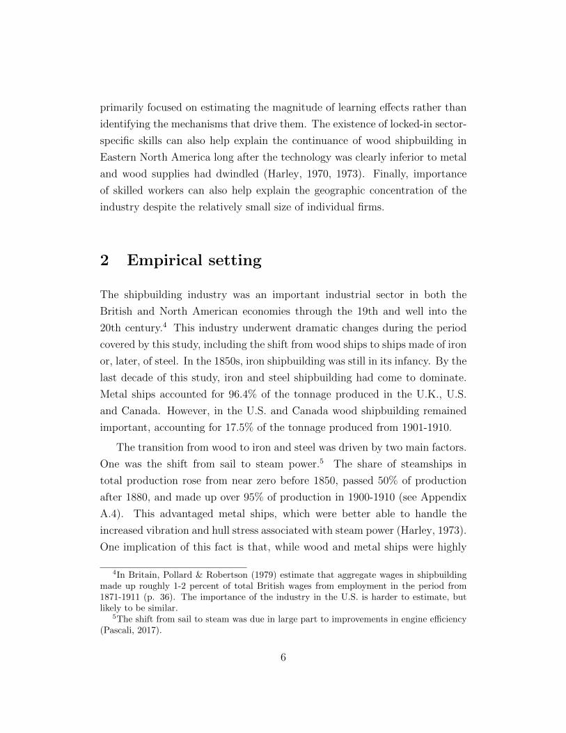
1. Further data on this point from the Census of 1900, presented in Table 1,

show that there were no systematic differences between iron and wood prices

on the Great Lakes compared to the Atlantic Coast. While iron prices were

relatively low in some Lakes states, like Illinois, they were high in others, such

as Michigan and Ohio. Similarly, there is no evidence that Atlantic coast

producers had a relative advantage in wood prices.

14Thompson writes (p. 45), “The larger foreign-built ships, those too long to negotiate thelocks in the Welland or St. Lawrence...had their midbodies removed, and the remaining bowand stern sections were welded together. With the midbody sections stowed in their cargoholds, the downsized ships made their way through the locks...Once above the Welland, thevessels would again be cut in half and the midbody sections reinstalled before the shipswere put into service.” The Annual Report to the Commissioners of the Navy (p. 15) saysof this method, “The experiment of building large vessels, cutting them in two to pass thelocks, and then reuniting the parts has been made successfully in a few instances, but atthe present time it does not appear that this method...will become general.” There arealso reports of ships that moved into the Great Lakes by going up the Mississippi river andthrough the Illinois and Michigan Canal, but this required that the ship’s have their entiresuperstructure removed in order to pass under the river bridges along the route. In addition,there were small metal vessels called canallers because they were built to be able to passthrough the small St. Lawrence and Welland Canals. Some of these made their way intothe Great Lakes in the 1890s, but these smaller ships were usually under 250 ft long.

11

Table 1: Iron and wood prices in some Atlantic and Great Lakes States, 1900

Notes: Data are from the the U.S. Census for 1900. See descrip-tion in Appendix A.9.

On the demand side, incentives for producing metal rather than wood ships

in the Lakes were also similar to on the coast. This is important because one of

the identifying assumptions in the main analysis is that there were no factors

that systematically increased the demand for metal ships relative to wood

ships (I do not need to assume that trends in overall demand for shipping

capacity were similar across locations). For example, the transition from sail

to steamships that took place in the Lakes was similar to the transition in the

Atlantic market as a whole, as described in Appendix A.4. The incentives for

using metal provided by opportunities to construct larger ships were actually

weaker in the Great Lakes than on the Coast, because, as shown in Appendix

A.6, maximum ship sizes in the Lakes remained smaller than in the Atlantic.15

On the other hand, metal ships did last longer on the Lakes because freshwater

was less corrosive, which may have provided some increased incentive for metal

ship production there. While ships on the Lakes did have different designs than

those on the coast, such as being longer and skinnier to maximize use of the

15The smaller size of ships on the Great Lakes was due to the limitations imposed bylocks and canals, particularly the lock between Lake Superior and the lower Great Lakes.

12

available locks, there doesn’t seem to have been any important differences in

the techniques used to construct lake ships.16

Industrial policy and protection from foreign competition played an im-

portant role in the shipbuilding industry, particularly in the U.S. One tool

used by the U.S. was a ban on the use of foreign-built ships for direct trade

between American ports (coastal trade). This policy, which existed through-

out the study period and continues today, created a protected market for

U.S. shipbuilders, though the size of this market was limited. Essentially, this

policy acts like a prohibitively high tariff on the import of ships for use in

the coastal trade. Given that foreign ships were effectively barred from the

coastal market while evidence suggests that U.S. shipbuilders primarily served

this protected market, I can use U.S. shipbuilding to get a sense of the size of

the protected market. This approach suggests that from 1901-1910 the pro-

tected U.S. coastal market accounted for about 1.7 million tons of production

or 8.7% of the total tonnage produced in the U.S., U.K. and Canada during

this period.

A second important channel of government influence on shipbuilding was

through the Navy. Warship construction gave domestic shipyards experience

and may have helped generate pools of skilled workers.17 From 1901-1910

the U.S. Navy bought vessels totaling 643,441 tons. While Navy vessels sizes

are measured in displacement tons, which is not directly comparable to the

tonnage measure for merchant vessels, this is roughly equivalent to about 3.3%

16One sign of the similarity of techniques used on the Lakes and the Coast is provided bythe Annual Report of the Commissioners of the Navy from 1901, which suggests that coastalshipbuilders may be able to learn from the more successful yards on the Great Lakes (p. 15):“...through the training of shipbuilders, the invention and improvement of shipbuilding tools,machinery, and materials, and through experience gained in the financial and industrialorganization of shipyards, the establishments on the Great Lakes are promoting the chancefor seaboard growth.”

17Hutchins (1948) suggests that the substantial expansion of the U.S. Navy in the late1880s and 1890s, often described as the “New Navy” because the new ships were metalrather than wood, played an important role in the development of U.S. shipbuilding. Ap-pendix A.10 describes the increases in U.S. Navy shipbuilding during the study period.Another type of industrial policy was the subsidization of passenger liners on mail-carryingroutes which had to be served with domestically-built ships. This form of protection wasparticularly important during the inter-war period.

13

of total U.S., U.K. and Canadian tonnage.

While the U.S. had access to the full range of protective policies, Canada,

as part of the British Empire, did not have the ability to enact similar poli-

cies. Specifically, Canada could not close coastal trade to British-built ships,

nor did it have an independent navy during this period to provide orders to

domestic yards or to operate government shipyards.18 As a result, data for

1912 show that 46% of the total tonnage homeported in Canada in that year

was constructed in the U.K. In contrast, only 7.6% of the tonnage homeported

along the U.S. coast was built in the U.K. Thus, comparing the experience of

the U.S. and Canada allows us to observe the evolution of this industry with

and without access to government protection.

While my analysis takes advantage of output market segmentation at the

regional level (U.S. Great Lakes, U.S. Coast, Canada Great Lakes, Canada

Coast), within these regions there was enormous heterogeneity across loca-

tions. The length of the Great Lakes stretches over 1000km West to East,

from Minnesota to New York State, and over 700km from North to South,

with over 7,000 km of coastline. Shipbuilding took place in large cities such as

Chicago, Toronto and Detroit, but also in many small out-of-the-way locations,

such as Thunder Bay, ON and Saugatuck, MI. Coastal shipbuilding in Canada

spanned a distance of over 1,600 km, from Montreal to St. John’s, Newfound-

land. On the U.S. Coast, shipbuilding locations stretched over 2,000km from

Maine to Florida. As a result, even within a region, individual shipyards faced

18Canada’s status as part of the British Dominion made enacting protection against themother country “scarcely thinkable” (Sager & Panting, 1990, p. 171). There were alsopractical difficulties. Sager & Panting (1990) explain that because Canada used the Britishregistration system for vessels, it was “virtually impossible to distinguish between Britishand Canadian ships, and hence a customs duty on British ships [in the Canadian foreigntrade] would be impossible to enforce.” Canada did have the ability to levy tariffs againstBritish imports, including imports of ships, but without being able to close ports to foreign-built ships tariffs on ships are ineffective at providing protection. If Canada placed a tariffon the purchase of British-built ships by Canadian shipping firms, the same ship could beused on the same route by a British owned shipping firm. Thus, without being able to lockBritish shipping firms out of the domestic market, the use of a tariff would only serve toshift the shipping business away from Canadian companies. In addition, the Royal CanadianNavy was not founded until 1910 and initially it was equipped with surplus vessels from theRoyal Navy, so this avenue of support was unavailable.

14

variation in input prices, availability and quality of shipyard space, labor mar-

ket conditions, etc. This is reflected in the wide variation in state-level input

prices within regions shown in Table 1, despite the fact that I do not observe

systematic differences in input prices across the regions. This variation moti-

vates my use of individual locations as the unit of analysis. The one factor that

tied together the heterogeneous set of shipyard locations within each region

was segmentation in the output market, the key source of variation exploited

in this study.

3 Data

The main analysis relies on a unique new data set derived from individual

ship listings on two registers, one produced by Lloyd’s and the other by the

American Bureau of Shipping (ABS, sometimes called “American Lloyd’s”).

The primary purpose of these registers was to provide insurers and merchants

with a rating of the quality of each ship. This provided shipowners with a

strong incentive to have their ship included on at least one major register,

and often more than one. As a result, the registration societies claimed that

the vast majority of major merchant ships (e.g., over 100 tons) were included

on one of the lists.19 The data cover only merchant ships; warships are not

included in the analysis. The vast majority of these were cargo carriers, though

the data also include passenger liners, some fishing and whaling vessels, and

other miscellaneous types (tugs, large barges, etc.).

The registers were published annually and included a variety of information

about each ship. Appendix Figure 7 provides an example of the data from the

first page of the Lloyd’s Register for 1871-72. From each register, I have

digitized the ship name, type (sail vs. steam), construction material (wood vs.

metal), tonnage, the location and year of construction, and in some cases the

19To be included on a register, a ship had to be inspected. This often occurred multi-ple times during the construction process and at periodic intervals after construction wascomplete. To complete these inspections, the registration societies employed a set of localinspectors in the majors shipbuilding areas of the world.

15

shipyard and current home port.20

This study uses data from registers for three years, 1871, 1889 and 1912.21

Because the registers include all active ships in these years, and because ships

generally last many years after construction, these snapshots provide coverage

for most ships built between 1850 and the First World War.22 Specifically, I use

the 1871 register to track ships built between 1850 and 1870, the 1889 register

to track ships built between 1871 and 1887, and the 1912 register to track

ships from 1888-1911.23 For each snapshot year I digitized both the Lloyd’s

Register and the ABS Register. Appendix Table 6 describes the number of

vessels included in the data from each of the registers used in this study.

The full data set includes just over 69,000 ships. Most of the analysis fo-

cuses on the subset of these built in the U.S. or Canada from 1851-1912. The

data required extensive processing to clean and standardize location names,

eliminate duplicate entries that appeared in both registers, identify the con-

struction material for each ship, etc. After eliminating duplicates, the main

analysis relies on observations for 21,809 ships built in the U.S. or Canada

between 1850 and 1912. Within the regions that I study, it is possible to iden-

tify the exact location of construction for the vast majority of ships.24 For the

main analysis the unit of observation is the location (city or town) of construc-

20The register also included additional information about the current owner, home portand master of each ship. These data were not entered for cost reasons. The home port ofeach ship was entered for the 1912 ABS Register only.

21The use of these snapshots is driven primarily by cost concerns. Digitizing each reg-ister requires entering data from thousands of pages of documents by hand, so even withoutsourcing this to low-cost providers the cost is substantial.

22The patterns over time described in my data are similar to those found in availableaggregate statistics (see Appendix A.3), which provides some confidence that the valuesderived from the registers are reasonable.

23The registers often did not have complete coverage for ships in the year in which theywere published.

24For ships built in the U.S. and Canada, I am able to identify the construction locationfor over 99% of ship tonnage in data from the 1912 register, over 96% of tonnage in the1889 registers. In data from the 1871 registers, the share of tonnage linked to a locationwithin the U.S. and Canada, respectively, is 97.1% and 88.3%. The larger share of tonnagewith missing locations in the Canadian data is due to the fact that only the province ofconstruction was provided for many Canadian ships registered in the 1871 Lloyd’s.

16

tion.25 Some summary statistics for the data on production by location used

in the main analysis are reported in Appendix Table 5. Maps of the data are

available in Appendix A.5.

In addition to the main data, I have also constructed several controls using

Census data. I control for nearby employment in metal-working or wood-

working industries using county-level Census data from the U.S. and Canada

in 1880 (see Appendix A.8 for details). These county data are not available for

Newfoundland so some observations are lost when these controls are included.

Controls for iron and lumber prices at the state level, available only for the

U.S., come from the Census of 1900. These are described in more detail in

Appendix A.9.

4 Main analysis

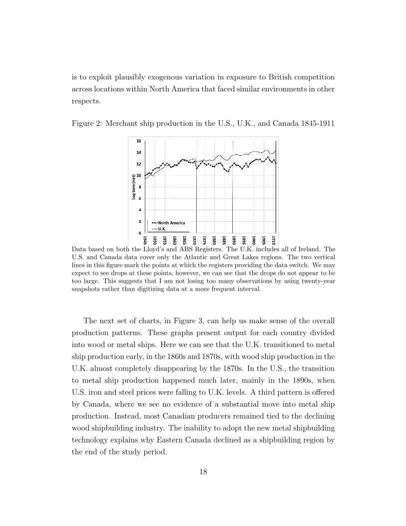
The starting point for the analysis is Figure 2, which describes overall ship

output in North America (U.S. and Canada) and Britain from 1845-1911. We

can see that North America was initially the largest shipbuilding area, but it

was soon surpassed by Britain. By the 1880s Britain dominated the market

and this continued up to WWI despite the fact that Britain’s input price

advantages essentially disappeared in the 1890s.

The key question posed by Figure 2 is why, after the price of metal in-

puts fell in the 1890s, North American shipbuilders were unable to catch up

to British production levels? One possible answer to this question is that

other factors made North America generally unsuitable for metal ship produc-

tion. An alternative answer is that the early lead enjoyed by British producers

made them more productive and that exposure to these more productive for-

eign competitors made it difficult for North American producers to adopt the

new metal shipbuilding technology. One way to evaluate these alternatives

25Most towns included just one shipyard, so this is somewhat close to a firm-level analysis,though more important locations could include multiple yards. I focus on locations ratherthan firms because firms are not well identified in the data and also to avoid the necessityof tracking firm ownership structures over time.

17

is to exploit plausibly exogenous variation in exposure to British competition

across locations within North America that faced similar environments in other

respects.

Figure 2: Merchant ship production in the U.S., U.K., and Canada 1845-1911

Data based on both the Lloyd’s and ABS Registers. The U.K. includes all of Ireland. TheU.S. and Canada data cover only the Atlantic and Great Lakes regions. The two verticallines in this figure mark the points at which the registers providing the data switch. We mayexpect to see drops at these points, however, we can see that the drops do not appear to betoo large. This suggests that I am not losing too many observations by using twenty-yearsnapshots rather than digitizing data at a more frequent interval.

The next set of charts, in Figure 3, can help us make sense of the overall

production patterns. These graphs present output for each country divided

into wood or metal ships. Here we can see that the U.K. transitioned to metal

ship production early, in the 1860s and 1870s, with wood ship production in the

U.K. almost completely disappearing by the 1870s. In the U.S., the transition

to metal ship production happened much later, mainly in the 1890s, when

U.S. iron and steel prices were falling to U.K. levels. A third pattern is offered

by Canada, where we see no evidence of a substantial move into metal ship

production. Instead, most Canadian producers remained tied to the declining

wood shipbuilding industry. The inability to adopt the new metal shipbuilding

technology explains why Eastern Canada declined as a shipbuilding region by

the end of the study period.

18

Figure 3: Shipbuilding tonnage by construction material

Panel A: U.K. production

Panel B: U.S. production

Panel C: Canadian production

Data based on both the Lloyd’s and ABS Registers.

19

Figures 2-3 describe the patterns that this study aims to understand. Next,

I provide graphical evidence describing the two key dimensions of variation

that I will use to isolate the impact of exposure to foreign competition on the

development of the North American industry.

Figure 4 looks at the share of output (by tonnage) of metal ships in the

U.K., on the Atlantic coast of the U.S. and Canada, and in the Great Lakes.

The key feature to note in this graph is the production pattern observed on the

Atlantic Coast of North American and the pattern observed in the Great Lakes.

While the share of metal ship production was similar in these two regions until

1880, after 1880 we can see that there was a dramatic shift. Shipbuilders in

the Great Lakes rapidly converged to the pattern of production observed in

the overall Atlantic market (U.K., U.S. and Canada) as the price of metal

inputs in North America fell, while this convergence process was much slower

among North American Atlantic Coast producers. Thus, this graph reveals

the impact of exposure to foreign competition on Atlantic Coast producers.

Figure 4: Evolution of production patterns by region

Data based on both the Lloyd’s and ABS Registers. The U.K. includes Ireland. The “AllAtlantic” category includes production in the U.K., U.S. and Canada.

Figure 5 compares shipbuilding in the U.S. and Canada to highlight the

20

role that exposure to British competition played in the transition from wood

to metal shipbuilding. The left-hand panel shows that, on the Atlantic Coast,

U.S. shipbuilders transitioned to metal more rapidly than Canadian builders.

In contrast, on the Lakes, where shipbuilders were more protected from for-

eign competition, the U.S. and Canada show similar patterns. These patterns

reflect the fact that the protection offered to U.S. shipbuilders was impor-

tant on the coast, while U.S. government support had less effect on the Great

Lakes, where producers were already protected from foreign competition by

geographic barriers.

Figure 5: Evolution of metal share on the Coast vs. the Lakes

Atlantic Coast Great Lakes

Data based on both the Lloyd’s and ABS Registers.

It is useful to consider why Canada and the U.S. exhibit roughly similar

patterns in the Great Lakes region despite the fact that U.S. Lakes shipbuilders

benefited from protection on routes between U.S. ports.26 The key to recon-

ciling this protection with the similar patterns shown in Figure 5 is to note

that while protection aided U.S. producers, it did not specifically benefit metal

ship production relative to wood ship production.27 Thus, it should not af-

fect relative production in these two sectors in the U.S. relative to Canada.

However, protection most likely did influence the relative level of production

26There were no Navy shipyards on the Great Lakes and no substantial Naval vessels wereproduced there.

27I.e., there is no evidence that U.S. Lakes producers were not substantially ahead orbehind Canadian Lakes producers in either sector.

21

between the two countries. In contrast, on the Atlantic Coast protection from

British competition specifically favored metal ship producers relative to wood

because it was in metal ships that producers faced stiff foreign competition.

Next, I turn to the econometric analysis. I begin by looking at the exten-

sive margin, i.e., whether locations were active in a particular sector (wood or

metal). I then turn to the intensive margin, i.e., the amount of tonnage pro-

duced conditional on being active. The first set of results are obtained from

cross-sectional regressions focused on the 1901-1910 period, after the input

price differences had largely disappeared. Later, I also consider the timing of

when protection mattered using the full panel of data.

I begin by looking at the extensive margin using multinomial logit (ML)

regressions. The specification is,

Als = 1[a∗ls > 0] (1)

a∗ls = α1LAKESl + α2UScoastl +XjsΓ + els

where Als is an indicator variable for whether location l is active in shipbuilding

sector s ∈ {wood,metal, both} in the 1901-1910 decade (with inactive as the

reference category), and a∗ls is an unobserved latent variable which depends on

the set of explanatory variables. LAKESl is an indicator variable for whether

the location is in the Great Lakes region while UScoastl is an indicator for

whether the location is on the Atlantic coast of the U.S. I treat these two

areas separately because they experienced varying levels of protection from

British competition.28 The reference region is Atlantic Canada, which was

fully exposed to foreign competition. The error term els follows a logistic

distribution.

Among the control variables that I consider is whether a location has been

28It is also possible to estimate separate effects for the U.S. and Canada in the GreatLakes region. These estimates, which are available in Appendix A.13 show similar resultsfor the U.S. and Canada in the lakes, which motivates pooling these locations in the mainspecifications.

22

active in shipbuilding in some past decade (typically 1871-80, which avoids

the decade of the U.S. Civil War but predates the input price convergence)

at all, or in sector s specifically, and if so, the tonnage produced in that past

decade in the location overall or in sector s specifically. These controls help

capture a location’s physical assets for ship production such as a deep harbor

or easier access to inputs. In some specifications I also control for shipbuilding

in other nearby locations, county-level employment in other metal industries

and lumber mills, and state-level iron and wood input prices.29

One potential identification concern in this study, as well as other studies

using a similar identification strategy, is that there could be some other time-

varying regional shock to treated locations, such as those in the Great Lakes,

that is not captured by the available control variables. In this study, the

availability of two sources of plausibly exogenous variation – comparing the

Great Lakes to the Atlantic and the U.S. to Canada – provides some protection

against such concerns.

One may also worry about spatial correlation in my regressions. To ex-

amine this possibility I have generated results clustering standard errors by

U.S. state or Canadian province for all of the main specifications. In general

this results in a slight reduction in the size of the estimated standard errors,

suggesting weak negative spatial correlation across shipbuilding locations. To

be conservative, I report robust standard errors in the main results tables. It is

worth noting that the fact that I observe evidence of weak negative spatial cor-

relation across locations suggests that treating these as separate observations

is a reasonable approach.

Table 2 presents ML regression results based on Eq. 1. These regressions

are run on the full set of U.S. and Canadian shipbuilding locations on the

East Coast or Great Lakes which were active at some point in the 1850-1910

period.30 Column 1 presents results without any additional controls while

29Shipbuilding in other nearby locations is based on data from the registers. County levelemployment data are from the 1880 Census. State level price data are from the 1900 Census.

30An alternative approach might be to run the analysis at the county level and include allcounties that bordered the lakes or the Atlantic. This approach requires that I take a stand

23

Columns 2-3 add in additional controls for activity in the location in the

1871-1880 decade, county level population and industry composition, and past

production in nearby locations.31 The results in Columns 1-3 suggest that

locations in the Great Lakes were more likely to be active in the production

of metal ships, either alone or in combination with wood shipbuilding, relative

to exiting the market. There is also some evidence that coastal locations in

the U.S. were more likely to remain active, but this result does not remain

significant as controls are added.

It is worth noting that adding in controls for previous production in Columns

2-3 affects the interpretation of the results. Without controlling for past pro-

duction patterns, the estimates in Column 1 should capture the impact of both

current protection from foreign competition as well as the effect of protection

in the past operating through learning effects. Adding in past production pat-

terns helps control for locational advantages in a particular type of shipbuild-

ing, but these controls will also soak up some of the effect of past protection

operating through learning. Since I am primarily interested in the impact of

protection in the period after which the gap between British and North Amer-

ican input prices had narrowed, my preferred results are those that include

controls for production patterns in the 1870s.

In Columns 4-5 I include additional controls for state-level iron and lumber

prices. Note that these data are available only for the U.S., which means that

fewer observations are available for these regressions and I cannot compare the

U.S. coast to Canada. Note that help reduce potential endogeneity concerns

with these controls I use prices for products in a relatively raw state (e.g., pig

iron and generic lumber) which are used as inputs in a wide variety of goods as

on counties suitable for shipbuilding. This determination is not as straightforward as itseems. For example, many shipbuilders located on rivers, while many coastal counties withrugged coastlines or in the north of Canada were unlikely shipbuilding locations. Thus,a sample of coastal counties is likely to include many counties that were unsuitable forshipbuilding, which really shouldn’t be in the sample.

31Of the controls included in the regressions in Table 2, the most explanatory are theindicators for whether a location was active in a particular sector in 1870. The otherconsistently significant control variable is county population, which is positively related towhether a location was active in both metal and wood ship production (outcome three).

24

well as shipbuilding, rather than inputs more directly related to shipbuilding

(e.g., steel plates).32 The fact that shipbuilding was only one of many uses

for these raw materials should limit endogeneity concerns. Despite the smaller

sample size I still tend to find evidence that locations in the Great Lakes were

more likely to be active in metal shipbuilding than those on the coast. It

is worth noting that these results are identifying the effect of the additional

protection provided by being in the Great Lakes (and in the U.S.) compared

to being in the U.S. but on the coast.

At the bottom of the table I include additional tests comparing the proba-

bility of being active in metal shipbuilding or in both sectors to the probability

of being active in wood shipbuilding alone. These tests are important because

comparing metal to wood ship production in the Great Lakes helps me deal

with concerns that the results are just reflecting more rapid growth in ship-

building in the Great Lakes overall. In general the effect of the Great Lakes on

whether a location is active in metal (in combination with wood) is statistically

different from the impact of the Great Lakes on activity in wood only.

The results in Table 2 are consistent with the idea that North American

shipbuilders that were not exposed to British competition were able to rapidly

switch to metal shipbuilding once metal input prices fell. This suggests that

it was exposure to initially advantaged British producers, rather than other

factors, that were likely behind the inability of Coastal North America ship-

builders to catch up to their British competitors after 1900.

Two additional sets of ML results are available in Appendix A.13. The

first considers both the ship’s construction material and power source (sail vs.

steam). These results show that Great Lakes producers were more likely to be

active in both metal sailing ship and metal steamship production. This shows

that differences in metal ship production between the Lakes and the Coast

were not driven by differences in demand for sailing vs. steamships. The

second set of results treats the U.S. and Canadian areas of the Great Lakes

regions separately and shows that both areas exhibit fairly similar patterns.

32See Appendix A.9 for further details.

25

Table 2: Multinomial logit regression results

(1) (2) (3) (4) (5)A=1: Location active in wood shipbuilding only in 1901-1910

U.S. Coastal -0.082 0.009 0.293(0.209) (0.228) (0.414)

Great Lakes 0.324 0.603 0.548 0.282 0.241(0.382) (0.418) (0.460) (0.610) (0.649)

A=2: Location active in metal shipbuilding only in 1901-1910

U.S. Coastal 0.630 1.049 0.321(0.712) (0.902) (1.064)

Great Lakes 2.991*** 1.671* 1.352 1.479* 1.790*(0.697) (0.848) (0.940) (0.737) (0.786)

A=3: Location active in both wood and metal shipbuilding in 1901-1910

U.S. Coastal 1.546* 2.554** 0.776(0.637) (0.842) (1.152)

Great Lakes 2.991*** 4.655*** 3.265** 3.423*** 2.873**(0.697) (0.941) (1.139) (0.815) (0.915)

Observations 833 833 779 274 274

Testing effect on A=2 different from A=1 (p-values)

U.S. 0.3315 0.2599 0.9801Great Lakes 0.0004 0.2420 0.4264 0.1832 0.1074

Testing effect on A=3 different from A=1 (p-values)

U.S. 0.0138 0.0030 0.6867Great Lakes 0.0004 0.0000 0.0224 0.0009 0.0107

Robust standard errors in parentheses. *** p<0.01, ** p<0.05, * p<0.1. Theanalysis covers all locations active in shipbuilding from 1850-1910 in in theAtlantic Coast or Great Lakes regions of the U.S. and Canada. Column 2 in-cludes controls for whether a location is active in metal or wood shipbuildingin 1870 as well as separate variables for tonnage produced in metal or woodin 1870. Column 3 adds additional controls for metal or wood shipbuilding atother locations within 100km, county log population, the county employmentshare in metalworking industries, and the employment share in lumber. Notethat the county data are not available for some locations. Column 4 includesthe controls in Column 2 together with the log price of pig iron and log lumberindex price in the state. These are only available for a subset of U.S. states,so the number of observations drops substantially. Column 5 includes the con-trols in Column 4 together with controls for county log population, the countyemployment share in metalworking industries, and the employment share inlumber.

Next, I study the intensive margin of production, i.e., how much tonnage a

26

shipyard produced from 1901-1910 in a particular sector conditional on being

active in that sector. The specification is,

ln(Yls) = β0METALs + β1LAKESl + β3UScoastl (2)

+ β4(METALs × LAKESl) + β5(METALs × UScoastl) +XjsΓ + εjs

where Yls is ship tonnage of type s produced in location l, METALs is an

indicator for the metal ship sector, and the remaining variables are defined

as before. The main coefficients of interest in this regression are β4 and β5

which reflect the impact of being in the Great Lakes market or in the U.S.,

respectively, on metal ship output relative to wood. I use log tonnage as

the dependent variable in these regressions, but similar results are obtained if

instead I use the level of tonnage (Appendix Table 15). This tells us that the

results are not being driven by the fact that the log specification places more

weight on smaller observations.

Table 3 presents the results of regressions based on Eq. 2. Column 1

presents baseline results while Columns 2-3 add in additional controls following

the same format as in Table 2. Columns 4-5 present results including state-

level price controls and using only observations from the U.S.33 These results

suggest that, conditional on a location being active in a particular sector,

tonnage of metal ship production was higher in locations in the Great Lakes

region and in the Coastal U.S. compared to Coastal Canada. The magnitudes

of these effects are large; being in the Great Lakes is associated with an increase

in tonnage of 4-5 log points relative to Coastal Canada and about 2 log points

relative to the Coastal U.S. (Columns 4-5). Being in the Coastal U.S. is

associated with a tonnage increase of about 2 log points relative to Coastal

Canada.34 Additional results, in Appendix A.14 show that these patterns are

33A version of the table displaying the estimated coefficients for all of the controls variablesis in Appendix A.14.

34Mean production in active metal shipbuilding locations in the data in 1901-10 was 66,000tons.

27

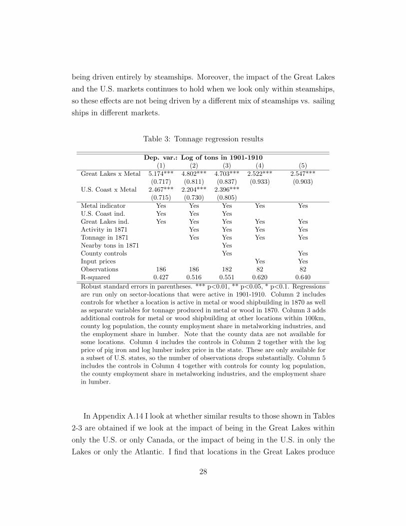
being driven entirely by steamships. Moreover, the impact of the Great Lakes

and the U.S. markets continues to hold when we look only within steamships,

so these effects are not being driven by a different mix of steamships vs. sailing

ships in different markets.

Table 3: Tonnage regression results

Dep. var.: Log of tons in 1901-1910(1) (2) (3) (4) (5)

Great Lakes x Metal 5.174*** 4.802*** 4.703*** 2.522*** 2.547***(0.717) (0.811) (0.837) (0.933) (0.903)

U.S. Coast x Metal 2.467*** 2.204*** 2.396***(0.715) (0.730) (0.805)

Metal indicator Yes Yes Yes Yes YesU.S. Coast ind. Yes Yes YesGreat Lakes ind. Yes Yes Yes Yes YesActivity in 1871 Yes Yes Yes YesTonnage in 1871 Yes Yes Yes YesNearby tons in 1871 YesCounty controls Yes YesInput prices Yes YesObservations 186 186 182 82 82R-squared 0.427 0.516 0.551 0.620 0.640

Robust standard errors in parentheses. *** p<0.01, ** p<0.05, * p<0.1. Regressionsare run only on sector-locations that were active in 1901-1910. Column 2 includescontrols for whether a location is active in metal or wood shipbuilding in 1870 as wellas separate variables for tonnage produced in metal or wood in 1870. Column 3 addsadditional controls for metal or wood shipbuilding at other locations within 100km,county log population, the county employment share in metalworking industries, andthe employment share in lumber. Note that the county data are not available forsome locations. Column 4 includes the controls in Column 2 together with the logprice of pig iron and log lumber index price in the state. These are only available fora subset of U.S. states, so the number of observations drops substantially. Column 5includes the controls in Column 4 together with controls for county log population,the county employment share in metalworking industries, and the employment sharein lumber.

In Appendix A.14 I look at whether similar results to those shown in Tables

2-3 are obtained if we look at the impact of being in the Great Lakes within

only the U.S. or only Canada, or the impact of being in the U.S. in only the

Lakes or only the Atlantic. I find that locations in the Great Lakes produce

28

more metal ship tonnage in 1901-1910 in both the U.S. and Canada, but the

protection afforded by the lakes is more important for Canadian shipbuilders.

Focusing only on the Atlantic Coast, I find evidence that shipyards in the U.S.

produced more metal ship tonnage, while I find no strong evidence that being

in the U.S. mattered in the protected Lakes market.

Next, I look at the timing of the effects using the full panel of data, focusing

on the intensive margin of production. The specification is,

Ylst =∑t

β0t(METALs ×Dt) +∑t

β1t(LAKESl ×METALs ×Dt)

+∑t

β2t(LAKESl ×WOODs ×Dt) +∑t

β3t(USl ×METALS ×Dt) (3)

+∑t

β4t(USl ×METALS ×Dt) +XjstΓ +∑t

ηtDt + φls + εjs

where Ylst is ship tonnage, WOODs is an indicator variable for the wood

shipbuilding sector, Dt is a set of indicator variables for each decade, and φls

is a set of fixed effects for each sector-location. These regressions allow me

to look at the impact of being in the Great Lakes or in the U.S. on iron ship

output while controlling for changes in output over time as well as differences

in regional production patterns over time. Because we may be concerned about

serial correlation in these regressions, standard errors are clustered by sector-

location. I focus on tonnage rather than log tons in this specification to avoid

dropping observations for locations that were inactive (produced zero tons) in

at least some decades.

The coefficients of interest in Eq. 3 are the vectors β1t - β4t, which reflect the

impact of being in the Great Lakes or being in the U.S. in each decade within

each ship type. These estimates, together with 95% confidence intervals, are

described in Figure 6. The top panel shows the coefficients estimated for each

decade on the interaction between the Great Lakes and either metal or wood

shipbuilding. These results suggest that being located in the Great Lakes

was, if anything, associated with lower production tonnage prior to the 1880s.

29

Then, starting in the 1890s, there was a relative increase in tonnage produced

on the Great Lakes which was concentrated in metal shipbuilding. This timing

corresponds with the fall in U.S. iron and steel prices as well as an increase

in demand for Great Lakes shipping. In the bottom panel of Figure 6, we see

that starting in the 1890s metal shipbuilding experiencing a relative increase

in the Coastal U.S. compared to Coastal Canada. This timing corresponds to

the fall in metal prices and the expansion of the U.S. Navy.

Figure 6: Panel data regression results

Coefficients for Lakes × Metal and Lakes × Wood

Coefficients for U.S. × Metal and U.S. × Wood

Estimates based on decadal data from 1850-1910. Figures show coefficients for the interac-

tion of an indicator for metal shipbuilding with an indicator for the Great Lakes (top panel)

or the U.S. (bottom panel) and similar coefficients for interactions using an indicator for

wood shipbuilding. Regressions include decade effects and a full set of location-by-sector

fixed effects. Confidence intervals based on standard errors clustered by sector-location.

30

The main conclusion to draw from this section is that exposure to compe-

tition from initially advantaged British producers substantially retarded the

ability of North American shipbuilders to transition to metal ship produc-

tion. Whether this transition was made determined the ultimate success of

the industry in each location as wood shipbuilding disappeared in the early

20th century. Thus, exposure to initially advantaged competitor, rather than

some other factor, appears to have been the key determinant of whether North

American producers were able to transition to metal shipbuilding.

5 Evidence of learning

The results in the previous section suggest that North American shipyards were

unable to compete with British producers even after Britain’s initial advantage

in input prices had disappeared. One explanation for this pattern is that

the shipbuilding industry may be characterized by dynamic learning effects,

so that current productivity is increasing in previous production experience.

Such effects would explain why Britain’s initial lead meant that, later on,

North American shipyards exposed to British competition had trouble entering

metal shipbuilding. While existing evidence suggests that learning is a feature

of the shipbuilding industry (e.g., Thompson (2001), Thornton & Thompson

(2001)), that evidence comes from a very specific setting during wartime in

which shipyards sought to rapidly produce many ships with a common design.

This differs from the peacetime industry, where shipyards rarely produced

more than a couple of ships of each type. In addition, no clear evidence exists

on whether learning was confined within shipyards or whether it spilled over

into other nearby producers.35

In this section I seek to provide new evidence on learning in this indus-

try. As a first step, I look at the relationship between current output and

cumulative past production using an approach similar to the existing litera-

35This issue has been studied by Thornton & Thompson (2001), but their analysis usesa relatively small number of geographically dispersed yards which makes it impossible forthem to look for evidence of geographically localized spillovers.

31

ture.36 The results of this exercise, presented in Appendix A.15, show two

main results. First, metal ship production in a yard in 1901-1910 is positively

related to cumulative previous output in the yard with an elasticity ranging

from 0.157-0.195.37 While this estimate comes with several caveats, the mag-

nitude is similar to the estimates obtained in previous work.38 Second, and

more important for my purposes, there is evidence that output in a yard from

1901-1910 is positively related to cumulative past production in nearby loca-

tions within 50km. This effect is localized and dies out when we look from

50-100km. This provides some preliminary evidence that the industry was

characterized by geographically localized learning effects.

Next, I attempt to provide some better-identified causal evidence of learn-

ing effects by focusing on the impact of proximity to U.S. Naval Shipyards.

Proximity to Naval shipyards could benefit private-sector shipyards through

technology spillovers or by providing access to pools of skilled metal ship-

builders. Also, proximity may have improved access to Navy contracts, which

could have had beneficial effects that spilled over into the construction of mer-

chant ships within yards.39 The key identification assumption in this analysis

36This exercise is in the spirit of previous work such as Thompson (2001), though, impor-tantly, it is not possible to control for input usage in my setting. This raises the concern thatcumulative output may just be capturing the impact of factors such as installed shipbuildingcapacity. To help address this issue, and to highlight the localized nature of learning, I con-sider both the impact of cumulative production within a location as well as the additionalinfluence of cumulative production in nearby areas. Looking at effects across nearby loca-tions can help me avoid conflating the effects of learning from factors such as fixed capitalinvestments, though there remains a concern that this relationship may reflect fixed localadvantages in a particular shipbuilding sector. Thus, it is important to recognize that theseare merely exploratory regressions and not cleanly identified causal effects.

37Interestingly, I do not observe statistically significant evidence of a similar pattern inwood shipbuilding, a sector where I am not aware of any previous estimates. This may reflectthe fact that wood shipbuilding was a mature declining industry, while metal shipbuildingwas growing during this period.

38Thompson (2001) estimates an elasticity between output and cumulative past produc-tion of 0.21-0.26, while controlling for capital and labor inputs. One reason why I mayobserve a smaller elasticity despite the fact that I cannot control for input usage is that myanalysis covers a wide variety of different ship types, while Thompson’s analysis looks atlearning within one ship type.

39Using data on Navy contracts from Smith & Brown (1948) I do find evidence that U.S.coastal shipyards that were within 50km of Navy shipyards were more likely to obtain Navycontacts and that these locations produced more metal ship tonnage. Given this, it may

32

relies on the fact that these locations were not chosen because of specific advan-

tages in metal, relative to wood, shipbuilding. This is a plausible assumption

because the locations of the Navy shipyards in operation during the period

that I study (shown in the map in Appendix Figure 19) were all determined

around 1800, well before the introduction of metal ships.40 Thus, while Naval

shipyards were situated in locations with advantages for shipbuilding overall,

there is little reason to believe that they were sited in locations that were

particularly advantageous for metal shipbuilding after 1880.

Results looking at the impact of proximity to U.S. Navy shipyards are pre-

sented in Table 4. These are based on the set of U.S. Atlantic Coast shipyards

only. The regressions are run using log tonnage regression specification from

Eq. 2. Columns 1-3 present results using all U.S. Atlantic coast locations. In

Columns 5-6 I drop all locations within Pennsylvania, New York, New Jersey,

and Massachusetts. This helps address concerns that results may be due to

the fact that three of the Naval shipyards were located in the major cities of

Boston, New York and Philadelphia.41 All of the results suggest that close

proximity to a Naval shipyard – within 50km – has a positive impact on ton-

nage of metal ships produced. The impact of proximity to naval shipyards

on wood shipbuilding tends to be negative, suggesting that private shipyards

near the Navy yards were more likely to switch from wood to metal ship con-

struction, or that metal shipbuilding pushed wooden shipbuilding out of these

locations.

be tempting to include contracts as a control in the regressions. However, the awarding ofNavy contracts is also likely to be endogenous to success in metal merchant ship production,which suggests that including these contracts as controls is not the right approach.

40The five Naval shipyards in operation during the period I study were in Portsmouth, VA(Norfolk NSY, opened 1767), Boston, MA (opened 1800), New York City (Brooklyn NSY,opened 1800), Philadelphia (opened 1801), and Kittery, ME (Portsmouth NSY, opened1800). The only other early Atlantic shipyard, in Washington, DC, was opened 1799 butthis yard largely ceased ship construction after the War of 1812 because the AnacostiaRiver was too shallow to accommodate larger vessels. A Coast Guard shipyard was openedin Baltimore in 1899, but I do not include that in my analysis because it is likely that thelocation of that yard was influenced by Baltimore’s potential for metal shipbuilding.

41The results are also robust to dropping, individually, other major Atlantic Coast ship-building states such as Connecticut, Maine, Maryland or Virginia. Thus, it does not appearthat they are being driven by any one state.

33

Table 4: Results looking at the impact of proximity to U.S. Navy Shipyards

Using all Atlantic locations Dropping NY, PA and MA(1) (2) (3) (4)

Navy yard within 50km -1.178** -1.280*** -0.737 -0.847(0.472) (0.369) (0.705) (1.061)

Navy yard within 2.761** 2.381** 3.093** 4.456*50km x Metal (1.064) (1.005) (1.435) (2.608)

Navy yard within 100km -1.065 -1.051(0.711) (1.070)

Navy yard within 100km -0.806 -2.108x Metal (1.338) (1.481)

Observations 89 89 89 59R-squared 0.281 0.463 0.504 0.360

Robust standard errors in parentheses. *** p<0.01, ** p<0.05, * p<0.1. Regressions are runon data from U.S. Atlantic Coast locations only. All regressions include controls for whetherthe sector was metal. The regressions in Columns 2-5 also include controls for whether alocation was active in 1871-1880, whether it was active in the same sector in 1871-1880, totaltonnage produced in the location in 1871-1880, and tonnage produced in the same locationand sector in 1871-1880. Regressions in Columns 4-5 include county-level controls for logpopulation, metalworking employment share and lumber milling employment share.

6 A Discussion of the Channels

Existing models suggest a number of channels through which an initial ad-

vantage could have persistent effects. These include productivity advantages

gained through learning-by-doing, as in Krugman (1987) and Young (1991),

or through R&D, as in Grossman & Helpman (1991). Initial advantages could

also generate persistence through achieving internal economies of scale. An-

other potential mechanism emphasizes the importance of workers, and in par-

ticular, the development of worker skills through on-the-job experience (Lucas,

1988, 1993; Stokey, 1991). This section briefly reviews available historical evi-

dence in order to shed light on the channels likely to be at work in the context

that I study.

Two of these channels can be discarded at the outset. An explanation based

34

on internal economies of scale is inconsistent with the highly competitive and

fragmented nature of the shipbuilding industry. Also, historical sources also

indicate that shipyards typically did not invest in R&D, most likely because

the highly competitive nature of the industry left them with little surplus to

invest, while the ease of copying give them little incentive.42

Of the remaining channels, available historical evidence points to the devel-

opment of pools of skilled metal shipbuilders as the key factor that translated

Britain’s initial advantages into a persistent lead. As Pollard & Robertson

(1979) write in their authoritative history of the British shipbuilding industry

(p. 129), “While foreign builders were able to choose better sites and de-

sign more efficient yards and shops, they were unable to overcome completely

the greater efficiency of British labor, an efficiency that in part derived from

Britain’s longer tradition as a producer of iron and steel steamships.”

One aspect of this channel was the vital importance played by skilled work-

ers in the industry. In British yards these workers made up 70-80% of the work-

force.43 A wide variety of specialized skills were required for the production

of large metal ships, including riveters, tinsmiths, boilermakers, carpenters,

plumbers, riggers, fitters and draftsmen.44 While some of these skilled were

also applicable in sectors other than shipbuilding (so called “amphibians”) and

others were used in both wood and metal ship production (e.g., carpenters and

riggers), many important skills were unique to metal shipbuilding. For exam-

ple, the skills involved in bending and shaping large metal plates into curved

and irregular shapes were unique, and vital, to metal shipbuilding. One fac-

tor that increased the importance of skills is the fact that the vast majority

42For example, Pollard & Robertson (1979) write that (p. 148), “Many improvements,if not most, however, were developed outside of the industry, in the steel-making, electri-cal products, or engineering industries...it was only necessary for the shipbuilders to adoptinnovations after the basic research had been done elsewhere. Few laboratories were estab-lished in the yards, and as the reluctance to use experimental tanks [to test ship designs]demonstrates, builders were not even very interested in investing funds to solve problemspeculiar to their industry.”

43Pollard & Robertson (1979) (Table 8.1, p. 153) show that in 1892 unskilled workersmade up 29% and 22% of the labor force in English and Scottish shipyards, respectively,18% in Scottish yards in 1911, and 25% in Northeast England in 1913.

44See Pollard & Robertson (1979) p. 78.

35

of ships were bespoke products produced to designs supplied by the buyer.45

This increased the need for skilled workers who could move flexibly between

different ship types.46

Skills were acquired primarily through experience. In Britain, this typically

meant formal apprenticeships lasting 5-7 years. Only a very small subset of

the most skilled workers, such as marine engineers and naval architects, had

any formal education.47

In contrast to British yards, evidence suggests that North American pro-

ducers wishing to begin metal shipbuilding in the late 19th century faced a

scarcity of experienced metal shipbuilders. Pollard & Robertson (1979) de-

scribe how, to compensate for the lack of skilled workers, North American

shipyards used more capital in order to substitute toward unskilled workers.

Unfortunately for these yards, “expensive equipment could not compensate for

the lower level of skills and more irregular output...Thus, despite Britain’s in-

ferior capital equipment, the output per man hour was still highest in Britain

at the end of the [19th] century.” While, “In the United States, vast over-

heads crippled builders in all but the best years. British yard owners were

able to take advantage of their more highly skilled workforces by investing

only in equipment that was absolutely necessary...and by refusing to purchase

as many labor-saving machines as German and American builders did.” Con-

sistent with this, Hutchins (1948) found that (p. 50), “American shipyard

work which could be effectively mechanized cost no more than that in Britain,

but handicraft work, of which there was a large amount, was much more ex-

pensive.” Thus, despite using more capital and advanced technology, evidence

suggests that the lack of skilled workers meant that the cost of producing

most merchant ship types in North American yards was much higher than in

45Pollard & Robertson (1979) write (p. 152), “..the fact that they [shipbuilders] producedfor the most part a large, custom-made commodity that was not susceptible to many of thetechniques of mass production, ensured that a premium continued to be placed upon skilledlabor.”

46This represents an important difference relative to the Liberty shipbuilders studied inprevious work, who focused on producing standardized designs.

47See Pollard & Robertson (1979) for more details.

36

Britain.48

Additional evidence on the scarcity of skilled metal shipbuilders in the U.S.

in the late 19th Century is offered by Hanlon (2018), which uses census data to

study the composition of the workforces in two U.S. Atlantic Coast shipyards

that successfully transitioned into metal shipbuilding: Newport News Shipyard

in Virginia and Bath Iron Works in Maine. That study shows that, early

in their life, these shipyards substituted away from skilled workers towards

unskilled workers and capital and relied on immigrants from Britain to fill key

skilled positions that could not be eliminated. Once established, these yards

began to train native-born workers to fill skilled positions.

One illustration of the challenges faced by North American shipyards is

provided by the 1905 Report of the Merchant Marine Commission to Congress.

This report provides the following example:

Convincing proof on this point was offered in 1900, when steel plates

and beams, because of labor troubles abroad, were selling at $40.86 in

England, and $28 in the United States. Boston shipowners at that

time invited bids from an American and a British builder for a cargo

steamship of about 5,000 tons capacity. With both yards figuring for

a small competitive profit, the American estimate was $275,000 and

the English $214,000. The material of the American ship would have

cost $63,000; of the English ship, $80,000. But this difference was

more than offset by the higher wages paid to the American shipyard

mechanics.

There is also evidence that a scarcity of skilled labor was the key constraint

in Atlantic Canada. For example, focusing on the Maritime Provinces, Sager

& Panting (1990) write that (p. 12), “The best contemporary estimates were

that Nova Scotia possessed all the necessary advantages for steel shipbuilding

except skilled labor.” This is a telling statement, particularly given that Nova

48Hutchins (1948), for example, suggests that (p. 47), “British costs were from 30 to40 percent less.” The Report of the Merchant Marine Commission found that in 1905 thedifference was 30 to 50 percent (p. viii).

37

Scotia had been one of the foremost (wood) shipbuilding areas in the mid-19th

century.

7 Conclusions

The experience of the international shipbuilding industry documented in this

study offers a window into understanding how temporary initial advantages

can influence long-run patterns of production and trade. My main results

show that initial input price advantages can have a long-run impact on the

spatial distribution of production and trade patterns. Due to lower input costs,

British shipbuilders were able to take an early lead in metal ship construction,

overcoming the dominant position that North American producers held in the

shipbuilding industry in the first half of the 19th century. Despite losing this

advantage in the 1890s, British producers were able to maintain their dominant

position in metal shipbuilding into the 20th century, while North American

firms that were exposed to competition from British producers struggled to

make the transition from wood to metal.

A natural explanation for this pattern is that the industry was character-

ized by some sort of dynamic learning effects. Previous work has already pro-

vided evidence that learning was important in ship construction (Thompson,

2001; Thornton & Thompson, 2001). Using the location of Navy shipyards,

I also document learning effects. In addition, my results suggest that learn-

ing spilled over across shipyards but that these spillovers were highly localized.

Such learning spillovers can explain how a temporary input cost advantage can

generate a persistent productivity advantage, as well as why successful metal

shipyards tended to be clustered in just a few locations. Finally, a review of

historical evidence suggests that the development of pools of skilled shipyard

workers was likely to have been a key channel through which these localized

learning effects operated.

38

References

Allen, R.C. 1977. The Peculiar Productivity History of American Blast Furnaces, 1840-1913.

The Journal of Economic History, 37(3), 605–633.

Allen, R.C. 1979. International Competition in Iron and Steel, 1850-1913. The Journal of

Economic History, 39(4), 911–937.

Allen, R.C. 1981. Accounting for Price Changes: American Steel Rails, 1879-1910. Journal

of Political Economy, 89(3), 512–528.

Argote, L, Beckman, SL, & Epple, D. 1990. The Persistence and Transfer of Learning in

Industrial Settings. Management Science, 36(2), 140–154.

Bardhan, P. 1971. On Optimum Subsidy to a Learning Industry: An Aspect of the Theory

of Infant-Industry Protection. International Economic Review, 12(1), 54–70.

Bleakley, Hoyt, & Lin, Jeffrey. 2012. Portage: Path Dependence and Increasing Returns in

U.S. History. Quarterly Journal of Economics, 127(May), 587–644.

Dunmore, W.T. 1907. Ship Subsidies. Houghton Mifflin Company.

Grossman, G, & Helpman, E. 1991. Innovation and Growth in the Global Economy. Cam-

bridge, Massachusetts: The MIT Press.

Hanlon, WW. 2018. Skilled immigration and American Industrialization: Lessons from the

Shipyards.

Harley, C. K. 1970. British Shipbuilding and Merchant Shipping: 1850-1890. The Journal

of Economic History, 30(1), pp. 262–266.

Harley, C. K. 1973. On the Persistence of Old Techniques: The Case of North American

Wooden Shipbuilding. The Journal of Economic History, 33(2), pp. 372–398.

Head, Keith. 1994. Infant industry protection in the steel rail industry. Journal of Interna-

tional Economics, 37(34), 141 – 165.

Hutchins, John G.B. 1948. The Shipbuilding Business in the United States of America. The

Society of Naval Architects and Marine Engineers. Chap. 2: History and Development

of the Shipbuilding Industry in the United States, pages 14–60.

Irwin, Douglas A. 2000. Did Late-Nineteenth-Century U.S. Tariffs Promote Infant Indus-

tries? Evidence from the Tinplate Industry. The Journal of Economic History, 60(2),

pp. 335–360.

Irwin, Douglas A. 2003. Explaining America’s Surge in Manufactured Exports, 1880-1913.

The Review of Economics and Statistics, 85(2), pp. 364–376.

Jacks, D. S., & Pendakur, K. 2010. Global Trade and the Maratime Transport Revolution.

Review of Economics and Statistics, 92(4), 745–755.

Jacks, D. S., Meissner, C. M., & Novy, D. 2008. Trade Costs, 1870-2000. The American

Economic Review, Papers & Proceedings, 98(2), pp. 529–534.

Juhasz, Reka. 2014 (November). Temporary Protection and Technology Adoption: Evidence

from the Napoleonic Blockade. Working Paper.

39

Krueger, A.O., & Tuncer, B. 1982. An Empirical Test of the Infant industry Argument.

American Economic Review, 72(5), 1142–1152.

Krugman, P. 1987. The Narrow Moving Band, the Dutch Disease, and the Competitive

Consequences of Mrs. Thatcher. Journal of Development Economics, 27(1-2), 41–55.

Lane, N. 2016 (December). Manufacturing Revolution: Industrial Policy and Networks in

South Korea. Working paper.

Lucas, Robert E. 1988. On the Mechanics of Economic Development. Journal of Monetary

Economics, 22(1), 3–42.

Lucas, Robert E. 1993. Making a Miracle. Econometrica, 61(2), 251–272.

Matsuyama, Kiminori. 1992. Agricultural Productivity, Comparative Advantage, and Eco-

nomic Growth . Journal of Economic Theory, 58(2), 317–334.

Melitz, M. 2005. When and How Should Infant Industries be Protected? Journal of

International Economics, 66, pp. 177–196.

Mitchell, B. R, & Deane, P. 1962. Abstract of British Historical Statistics. London: Cam-

bridge University Press.

Pascali, Luigi. 2017. The Wind of Change: Maratime Technology, Trade and Economic

Development. American Economic Review, 107(9), 2821–2854.

Pollard, S., & Robertson, P. 1979. The British Shipbuilding Industry, 1870-1914. Cambridge,

MA: Harvard University Press.

Rapping, Leonard. 1965. Learning and World War II Production Functions. The Review of

Economics and Statistics, 47(1), 81–86.

Redding, S. 1999. Dynamic Comparative Advantage and the Welfare Effects of Trade.

Oxford Economic Papers, 51, 15–39.

Sager, Eric W., & Panting, Gerald E. 1990. Maratime Capital. Montreal: McGill-Queen’s

University Press.

Searle, Allan D. 1945. Productivity and Labor in Industry. Monthly Labor Review, Decem-

ber, 1132–47.

Smith, H.G., & Brown, L.C. 1948. The Shipbuilding Business in the United States of Amer-

ica. New York, NY: The Society of Naval Architects and Marine Engineers. Chap. 3:

Shipyard Statistics, pages 61–200.

Stokey, N. 1991. Human-Capital, Product Quality, and Growth. The Quarterly Journal of

Economics, 106(2), pp. 587–616.

Thompson, Peter. 2001. How Much Did the Liberty Shipbuilders Learn? New Evidence for

an Old Case Study. Journal of Political Economy, 109(1), pp. 103–137.

Thompson, Peter. 2005. Selection and Firm Survival: Evidence from the Shipbuilding

Industry, 1825-1914. The Review of Economics and Statistics, 87(1), pp. 26–36.

Thompson, Peter. 2007. How much did the Liberty shipbuilders forget? Management

Science, 53(6), 908–918.

Thornton, R. A., & Thompson, P. 2001. Learning from Experience and Learning from Oth-

40

ers: An Exploration of Learning and Spillovers in Wartime Shipbuilding. The American

Economic Review, 91(5), pp. 1350–1368.

Young, Alwyn. 1991. Learning By Doing and the Dynamic Effects of International Trade .

Quarterly Journal of Economics , 106(2), 369–405.

41

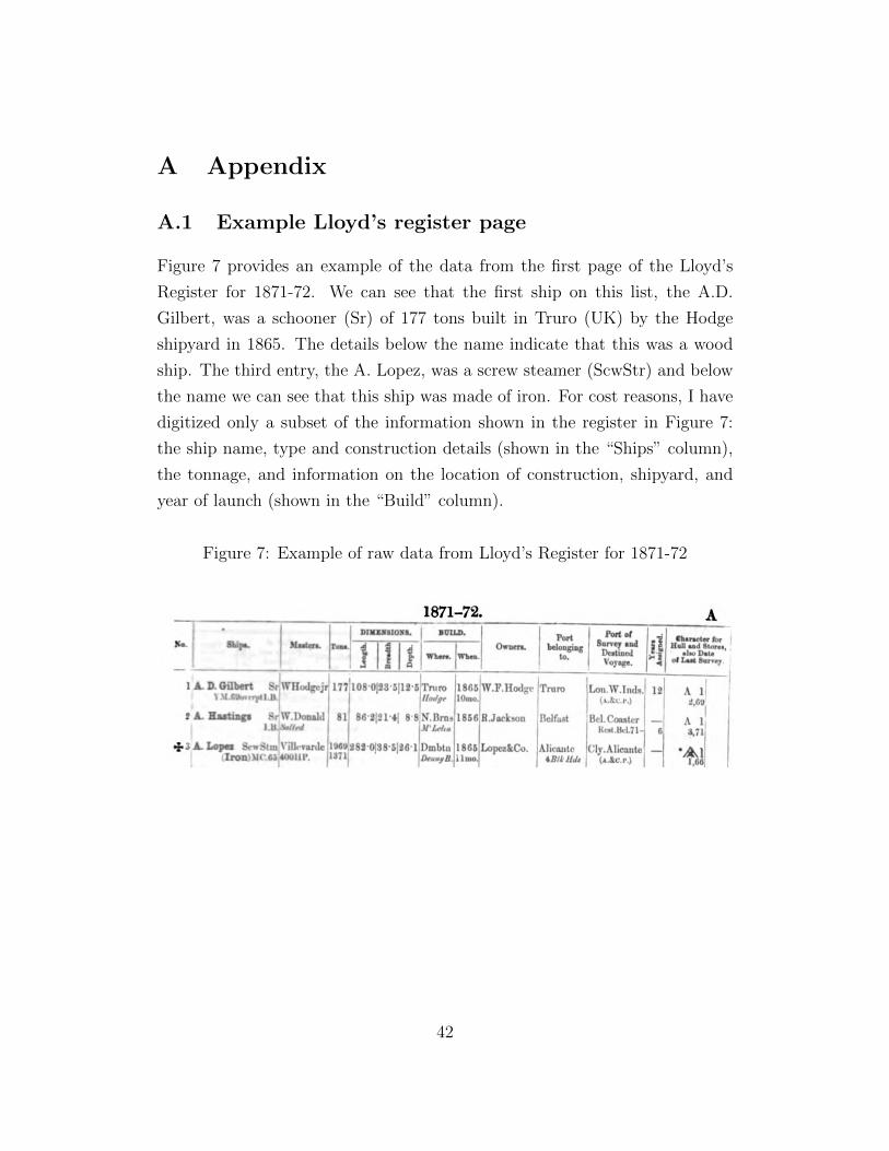
A Appendix

A.1 Example Lloyd’s register page

Figure 7 provides an example of the data from the first page of the Lloyd’s

Register for 1871-72. We can see that the first ship on this list, the A.D.

Gilbert, was a schooner (Sr) of 177 tons built in Truro (UK) by the Hodge

shipyard in 1865. The details below the name indicate that this was a wood

ship. The third entry, the A. Lopez, was a screw steamer (ScwStr) and below

the name we can see that this ship was made of iron. For cost reasons, I have

digitized only a subset of the information shown in the register in Figure 7:

the ship name, type and construction details (shown in the “Ships” column),

the tonnage, and information on the location of construction, shipyard, and

year of launch (shown in the “Build” column).

Figure 7: Example of raw data from Lloyd’s Register for 1871-72

42

A.2 Description of the Register data

Table 5 presents some basic statistics for the decades 1871-1880 and 1901-1910.

The later is the main focus of the analysis while the former provides a useful

benchmark that falls after the disruptions cause by the U.S. Civil War but

before substantial convergence in input prices had taken place.

Table 5: Summary of tonnage and active locations in 1871-80 and 1901-10

Country Region Material Tons Active locations1870 1900 1870 1900

U.S. Atlantic Metal 102,243 1,216,970 8 21U.S. Atlantic Wood 644,837 478,305 212 68U.S. Lakes Metal 194 2,332,268 1 12U.S. Lakes Wood 1,036 6,387 5 11Canada Atlantic Metal 2,303 5,861 3 6Canada Atlantic Wood 610,911 72,283 260 57Canada Lakes Metal 0 84,427 0 4Canada Lakes Wood 1,878 3,996 5 7

Table 6 describes the number of observations from each register divided

into the U.S., Canada, U.K. and other locations. The data from the 1871

register cover the years 1850-1871, the 1889 register data cover 1871-1887, and

the 1912 data are used for years 1888-1912. Note that the data in Table 6

do not include thousands of other entries from these registers that fall outside

of the windows covered by each one. For example, the 1871 registers contain

over 2,000 ships built before 1850 that are not included in the tallies.

It is worth noting that there appear to be some entries in, say, the 1912

registers that for years before 1889 that are not included in the 1889 register.

Thus, in principal the additional data in the 1912 registers could be used to

fill in some missing observations for the period before 1889. However, doing so

raises the possibility of generating duplicate entries, particularly because ship

names change over time. Because of this possibility I have chosen not to use

the 1912 data to augment the set of observations for the years before 1889.

43

Table 6: Number of vessels in each Register used in this project

Total No. vessels by location of build:Year Register number of

ships U.S. Canada U.K. Others1871 Lloyd’s 8,521 100 1,086 6,879 456

ABS 12,185 5,594 2,547 1,502 2,542

1889 Lloyd’s 8,620 11 278 7,429 902ABS 8,478 3,326 2,052 548 2,552

1912 Lloyd’s 23,482 2,485 581 12,893 7,524ABS 8,164 3,418 331 3,464 951

The counts from the 1871 registers include entries for ships built from 1850-1870. The 1889 register entries include ships built from 1871-1887. The 1912entries include ships built from 1888-1911.

44

A.3 Aggregate tonnage data from alternative sources

Figures 8 and 9 present aggregate data series on shipbuilding output in the

U.S. and U.K. We can compare the patterns observed in Figure 2, which

come from the Registers. Overall, the patterns observed in the two series are

quite comparable, which provides some confidence that the Register data are

doing a good job of capturing industry production. Note, however, that the

actual tonnage values are not strictly comparable across these series. There are

several reasons for this. First, aggregate statistics generally cut off ships below

a certain tonnage level, but they are often not explicit about exactly what the

cutoff is. Some types of ships, such as barges, may also be excluded. Second,

many of the available aggregate statistics include only vessels that were both

produced in a country and then subsequently registered in that country. Third,

there are often differences in the type of tonnage measure between the registers

and the aggregate statistics. In general, the registers used a measure called

net tonnage, while many aggregate statistics, particularly for the U.S., use

gross tonnage. Unfortunately the relationship between gross and net tonnage

is different for each vessel, so there is no way to easily translate between them.

For a further discussion of tonnage measurement issues see Appendix A in

Pollard & Robertson (1979).

In general the patterns shown in Figure 8 look similar to those in Figure 2

in the main text. For example, both data series show total tonnage in the U.K.

surpassing output in the U.S in 1857. Other patterns, such as the depression

in 1886-87 and the spike in output in 1906-07 also look fairly similar. There

are also many similarities between the patterns observed in Figure 3 in the

main text and those shown in Figure 9. For example, both series show that

U.K. metal ship output exceeded wood ship output around 1861-82. However,

the series in Figure 9 do suggest that U.S. metal ship output grew more slowly

relative to wood ship output than I observe in the data used in the main text

in the 1890s. One explanation for this may be that some U.S. metal ships

were being sold abroad. Another explanation is that wood ships may have

been taken out of service relatively sooner, which would cause them to not

45

appear in the 1912 Registers.

Figure 8: Merchant shipbuilding in the U.S. and U.K., 1850-1913

Notes: Data for U.K. shipbuilding registered in the U.K. are from Mitchell & Deane (1962).All U.K. data were reported in net tons. Data for the U.S. come from Hutchins (1948) andare reported in gross tons. These have been converted to net ton using a ratio of 1.5 grosstons to net ton which is derived by comparing U.K. output in gross tons and net tons usingdata from 1878-1911.

Figure 9: Merchant shipbuilding in the U.S. and U.K. by type, 1850-1913

Notes: Data for U.K. are from Mitchell & Deane (1962) and include only ships first registeredin the U.K. These data are reported in net tons. Data for the U.S. come from Hutchins (1948)and are reported in gross tons. These have been converted to net ton using a ratio of 1.5gross tons to net ton which is derived by comparing U.K. output in gross tons and net tonsusing data from 1878-1911. Composite ships are included with wood.

46

A.4 Evidence on the shift from sail to steam

Figure 10 describes the share of steamships in total ship output (by tonnage)

in the U.S., U.K., and Canada, across the study period. Steam powered ship

tonnage was almost insignificant prior to 1850, rose above 50% of total produc-

tion in the 1880s, and was dominant after 1900. This transition from sail to

steam was driven largely by improvements in engine efficiency (Pascali, 2017).

Next, Figure 11 compares the transition from sail to steam in the Great

Lakes to the transition that took place in the Atlantic market (defined as the

U.K. and Atlantic coast production the U.S. and Canada). We can see that

the Great Lakes lagged behind in the use of steamships until after 1880 and

then experienced a decade of rapid catch-up in the 1880s before settling to

levels that were similar to those observed in the Atlantic market as a whole

after 1890. After the 1890s the pattern of steamship construction in the Great

Lakes looked very similar to the pattern observed in the Atlantic market.

It is important in Figure 11 that we compare the Great Lakes to the At-

lantic market as a whole, rather than just North American producers on the

Atlantic Coast. This is because the fact that North American Coastal pro-

ducers remained concentrated on wood ship production also meant that they

produced fewer steamships, where wood construction was a disadvantage.

Figure 10: Share of steamship production

47

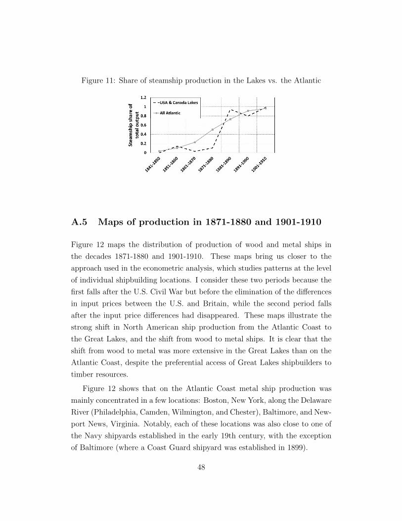
Figure 11: Share of steamship production in the Lakes vs. the Atlantic

A.5 Maps of production in 1871-1880 and 1901-1910

Figure 12 maps the distribution of production of wood and metal ships in

the decades 1871-1880 and 1901-1910. These maps bring us closer to the

approach used in the econometric analysis, which studies patterns at the level

of individual shipbuilding locations. I consider these two periods because the

first falls after the U.S. Civil War but before the elimination of the differences

in input prices between the U.S. and Britain, while the second period falls

after the input price differences had disappeared. These maps illustrate the

strong shift in North American ship production from the Atlantic Coast to

the Great Lakes, and the shift from wood to metal ships. It is clear that the

shift from wood to metal was more extensive in the Great Lakes than on the

Atlantic Coast, despite the preferential access of Great Lakes shipbuilders to

timber resources.

Figure 12 shows that on the Atlantic Coast metal ship production was

mainly concentrated in a few locations: Boston, New York, along the Delaware

River (Philadelphia, Camden, Wilmington, and Chester), Baltimore, and New-

port News, Virginia. Notably, each of these locations was also close to one of

the Navy shipyards established in the early 19th century, with the exception

of Baltimore (where a Coast Guard shipyard was established in 1899).

48

Figure 12: Ship production in the U.S. and Canada, 1871-80 and 1901-10

1871-1880

1901-1910

49

A.6 Maximum tonnage data

This appendix provides additional data on the maximum size of ships being

produced in a particular market, period, or ship type. As a starting point,

Figure 13 describes the evolution of maximum ship tonnage over time across

markets and ship types for the U.S., U.K. and Canada. In all periods the

largest ship was metal and constructed in the U.K. with the exception of

1841-1850, when the largest ship was made of wood and constructed in the

U.S. Over the study period maximum ship size increased dramatically, from

under 3,000 tons in 1841-1850 to over 30,000 tons after 1900. The unusual

jump in maximum ship size in 1851-1860 was due to the construction of the

Great Eastern, a massive one-off metal ship built in London with a size that

was unsurpassed until 1899.

Figure 13: Evolution of maximum ship size over time

Figure 14 describes the largest ship produced in each period by type of

construction (wood vs. metal). This graph makes it clear that the size of

wood and metal ships was similar through 1880 (with the exception of the

Great Eastern in 1851-60) but diverged substantially after that point, with

metal ships growing much larger. In the end the size of wooden ships was

constrained below about 4,300 tons across the entire study period and grew

very little from 1850-1910. This illustrates the advantage that metal afforded

in the construction of larger ships.

50

Figure 14: Evolution of maximum ship size by type of construction

Finally, Figure 15 describes maximum tonnage on the Atlantic Coast and

the Great Lakes. We can see that maximum ship size grew in all locations,

but less so on the Great Lakes. This was most likely a result of the limitation

placed on lake ships by the size of canals and water depths. Overall, this

suggests that, if anything, ship size should have generated stronger incentives

for metal construction on the coast than on the lakes.

Figure 15: Evolution of maximum ship size on the Coast vs. the Lakes

51

A.7 Comparing Canadian and U.S. input price trends

Figure 16 plots data describing the evolution of iron prices (top panel) and

wood prices (bottom panel) in Canada compared to the U.S. starting in the

1870s. Because the Canadian price series are only available as an index, I

convert the U.S. pig iron price series used in Figure 1 to an index. For both

indices, I set the prices from 1870-1879 to equal one.49 These data show the

similarity between Canadian and U.S. input price trends.

Figure 16: Iron and wood price trends in Canada and the U.S.

Iron prices

Wood prices

Notes: U.S. prices are from Historical Statistics of the United States, Colonial Times to1870, Vol. 1. I am grateful to Ian Kaey for sharing his Canadian price series with me.

49I use a full decade here to deal with the high level of price volatility in the 1870s, whichmeans that the picture can change substantially when using only a single base year.

52

A.8 Description of county employment controls

The analysis includes controls for county-level employment in metal industries

and lumber mills. These controls are constructed from the 1880 U.S. Census

and 1880 Canadian Census records. I focus on 1880 primarily for data rea-

sons, since I have not found county-level information on industry employment

for the U.S. for 1890 or 1900. Using 1880 data also has the advantage of

reducing endogeneity concerns, which may be an issue for controls based on

data for 1900. The U.S. Census data were collected by Martin Rotemberg and

Richard Hornbeck. The Canadian census data were entered from the original

manuscripts.

I have tried to produce series that are consistent across the two countries.

I focus on employment rather than output to avoid having to deal with ex-

change rates. For the U.S., the control for employment in metal industries

includes: blacksmithing, brassware, bronzeware, copperware, cutlery and edge

tools, fire-arms, hardware, iron and steel machinery, leadware, other machin-

ery, other brass, bronze and copper products, saws, and steam fittings and

heating apparatus. For Canada I include the following sectors: blacksmithing,

metal founding and machinery production, edge tools, boilermaking, engine

production, firearms, and saws. To control for wood employment, the U.S. se-

ries is “lumber and timber products” while the Canadian series is “saw mills.”

County employment data is not reported for Newfoundland or some loca-

tions in the northern part of Quebec. Thus, a few observations are lost when

these controls are included.

A.9 Input price data description

This section description of the sources of the in put price data presented in

Table 1. These data were gathered from the special industry reports included

in Section 3 of the U.S. Census reports from 1900. Below I describe how these

data series were constructed.

53

Pig iron price data

Pig iron price data at the state level were reported on p. 33-34 of the report

for that industry. While some price information are available for other iron and

steel products, including products such as metal plates that were particularly

important for the shipbuilding industry, I focus on pig iron prices for three

reasons. First, pig iron was a relatively homogenous product (compared to

more specialized metal products) that was widely produced. This improves the

comparability of price data across locations. Second, pig iron was a key input

into more specialized metal products used in shipbuilding. Third, pig iron was

used as an input into a wide variety of goods. This reduces the chance that

local prices could be endogenously affected by the local shipbuilding industry,

which may be a concern when focusing on more specialized products where a

large fraction of output was used by shipbuilders.

In addition to providing prices for 1900, the report also provided data for

1890 and 1880. Figure 17 graphs these prices by state, with the solid lines

corresponding to states bordering the Atlantic and the dotted lines used for

states in the Great Lakes (note that New York and Philadelphia border both

the Atlantic and the Lakes). We can see that iron prices fell across all of the

states in the sample. In 1880, iron prices were generally higher in the Great

Lakes states, but prices fell more rapidly in the Lakes, so that by 1900 there

was no systematic difference between iron prices in the Great Lakes states and

prices on the Atlantic Coast.

Because the iron prices are only available for a subset of the states used in

the analysis, I use information from nearby states in order to expand the set

of locations that can be analyzed when including a iron prices as a control.

Specifically, I use the iron price from New York as the price for Connecticut

and Rhode Island, the price from Virginia is used for North Carolina, the

price from Maryland is used for Delaware and the District of Columbia, and

the price from Georgia for South Carolina. The remaining U.S. states that

are included in the main analysis but dropped when the iron prices control is

included are Massachusetts, Maine, New Hampshire, and Florida.

54

Figure 17: Evolution of iron prices by state, 1880-1900

Lumber price data

The lumber price data are also drawn from the Census of 1900. These data

are more complicated to prepare than the iron price data because different

types of trees grow in different areas and these varieties have different quality

levels. To begin, I collected data from a set of the most important types

of lumber for shipbuilding: oak, pine, ash, white pine, spruce, poplar, and

hemlock. These prices come from the special report on lumber and were

provided by lumber producers, rather than users. All of these wood types

are produced by multiple states and overlap with other types, but no type is

produced everywhere, and I only observe the price of a variety in a location in

which it was produced. The data I collect span 47 states (all of the lower 48

states except North Dakota).

These varieties differ substantially in price. For example, oak is systemat-

ically more expensive while pine tends to be less expensive. It is reasonable

to expect that wood shipbuilders in a particular location built primarily using

the type of wood that was more readily available near them.

To build a consistent index of wood prices, I run the following regression,

Pis = α + φi + θs + εis

55

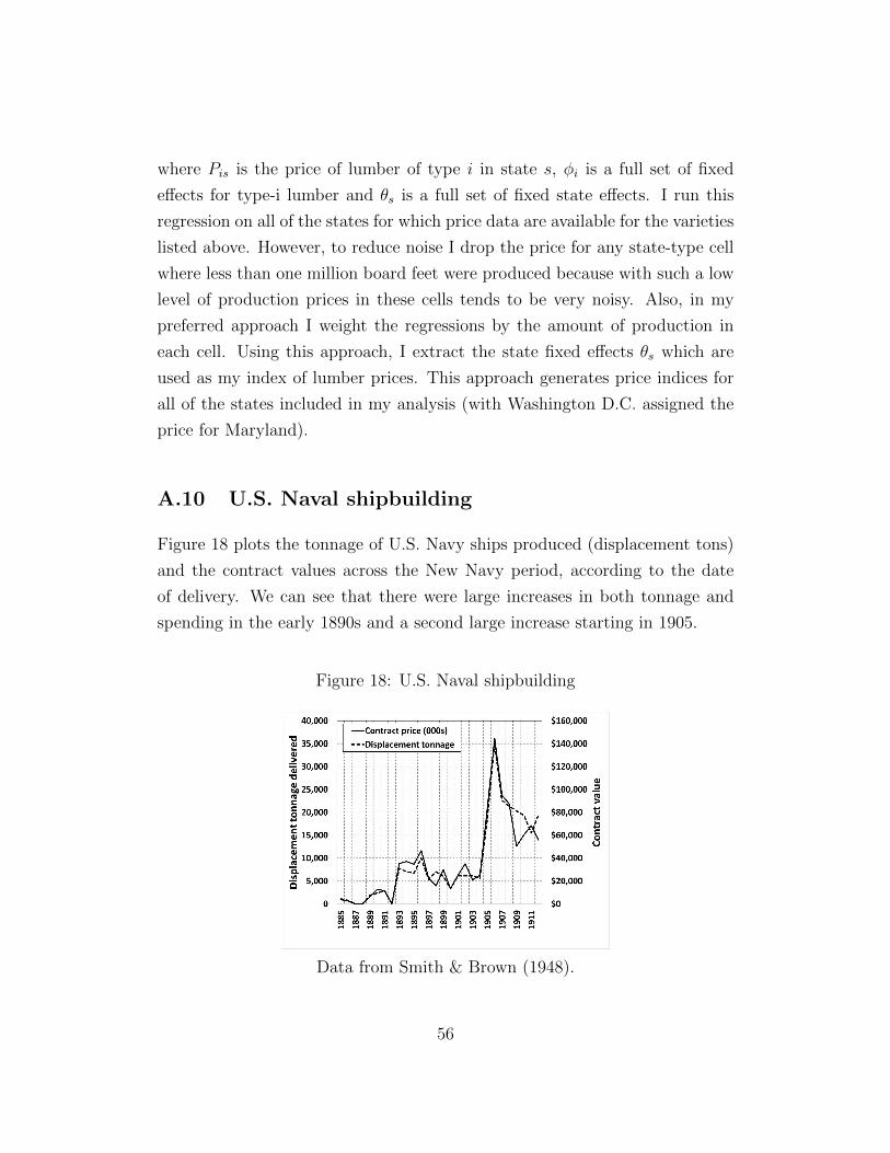
where Pis is the price of lumber of type i in state s, φi is a full set of fixed

effects for type-i lumber and θs is a full set of fixed state effects. I run this

regression on all of the states for which price data are available for the varieties

listed above. However, to reduce noise I drop the price for any state-type cell

where less than one million board feet were produced because with such a low

level of production prices in these cells tends to be very noisy. Also, in my

preferred approach I weight the regressions by the amount of production in

each cell. Using this approach, I extract the state fixed effects θs which are

used as my index of lumber prices. This approach generates price indices for

all of the states included in my analysis (with Washington D.C. assigned the

price for Maryland).

A.10 U.S. Naval shipbuilding

Figure 18 plots the tonnage of U.S. Navy ships produced (displacement tons)

and the contract values across the New Navy period, according to the date

of delivery. We can see that there were large increases in both tonnage and

spending in the early 1890s and a second large increase starting in 1905.

Figure 18: U.S. Naval shipbuilding

Data from Smith & Brown (1948).

56

A.11 Location of U.S. Navy Shipyards

Figure 19 plots the location of U.S. Navy shipyards, with 50km rings (solid

line) and 100km rings (dotted line) around each, together with the locations

of each of the Atlantic Coast shipyards active in the 1901-1910 period.

Figure 19: Map of the location of U.S. Navy Shipyards

57

A.12 Data comparing homeport and construction loca-

tions

Table 7 uses information on the homeport of ships entered from the 1912

ABS Register in order to compare construction locations and location of use.

The key take-away from this table is that the vast majority – 96.9% – of ships

homeported in the Great Lakes were also constructed in the Great Lakes. Also,

British ships accounted for only 1.3% of the Great Lakes tonnage registered

in the ABS. In contrast, only about 82.2% of the tonnage homeported on

the Atlantic Coast of the U.S. and Canada was also constructed there, while

British producers captured almost 10% of the market. Overall, these figures

suggest that the Great Lakes market was much more isolated from outside

competition than the Atlantic Coast market.

Table 7: Tonnage by construction location and homeport location

All data are derived from the 1912 ABS data and cover the years 1890-1912.

Table 8 provides some evidence on the penetration of foreign shipbuilders

into the U.S. and Canadian markets on the Atlantic Coast. We can see that

U.K. producers built 7.6% of the tonnage homeported on the Atlantic Coast

of the U.S., but 46% of tonnage on the coast of Canada. An additional 6%

of Canadian Atlantic ship tonnage came from U.S. producers, while Canadian

producer supplied less than 1% of U.S. tonnage. These figures reflect the

58

important role that U.S. trade protections likely had on the use of foreign

ships.

Table 8: Construction location for tonnage homeported on the Atlantic Coastof the U.S. and Canada

All data are derived from the 1912 ABS data and cover the years 1890-1912.

An alternative view of market segmentation is provided by Table 9, which

looks at the homeport locations of vessels constructed on in the Great Lakes

or on the Atlantic Coast of the U.S. and Canada. We can see that 94.4% of

the tonnage constructed on the Great Lakes is also homeported on the Great

Lakes, in either the U.S. or Canada. In contrast, only 83.5% of the tonnage

constructed on the Atlantic coast of the U.S. and Canada is also homeported

there, while 8.6% of tonnage is homeported in a foreign country. Again, this

highlights the much more closed nature of the Great Lakes market.

59

Table 9: Homeport locations for tonnage built in the Great Lakes or AtlanticCoast of the U.S. and Canada

All data are derived from the 1912 ABS data and cover the years 1890-1912.

A.13 Additional results for whether a location is active

This section presents some additional results looking at the factors that predict

whether a location was active in producing a particular type of ship (wood or

metal) in the 1901-1910 period. The first table shows results that allow the

production of sail vs. steam ships to be different choices. Thus, the outcome

variable can take five values: 0 if the location was inactive; 1 if the location

produced wood sailing ships; 2 if the location produced wood steamships; 3

if the location produced metal sailing ships; 4 if the location produced metal

steamships. To keep things tractable, I treat these as independent decisions.

This differs from the specification used in the main text, which considers the

joint production of iron and wood ships to be a different choice than producing

only iron.

One reason to consider this specification is that we may be concerned that

differences in the use of steamships between the Great Lakes and Coastal

regions may have contributed to differences in the use of metal vs. wood for

construction. Looking at the effect of being in the Great Lakes on production

of metal vs. wood ships within ship type can address this potential concern.

However, because we are dividing the data into smaller cells we should expect

60

this specification to deliver results with larger standard errors.

Table 10 presents ML regression results differentiating by both material

of construction and power source. Note that these results do not include the

specifications with controls for the iron and lumber prices. Doing so reduces

the sample size and makes it difficult to estimate reliable results when using

more categories.

In the top panel, we see that shipbuilders in the Great Lakes or in the

U.S. were not more likely to be active in building wood sailing ships. In the

second panel, we see evidence that both Great Lakes and U.S. shipbuilders

were more likely to be active in the construction of wood steamships. In the

third panel we see some evidence that Great Lakes producers were more likely

to be active in metal sailing ship production, though with few ships falling into

this category the results are not statistically significant. In the fourth panel,

the results show that both the Great Lakes and U.S. locations were more likely

to be active in metal steamship production. This result indicates that my main

findings continue to hold when looking only within steamships. At the bottom

I test for whether locations in the Great Lakes were more likely to be active

in metal steamships than in wooden steamships. In general this test suggests

that they were, though the results weaken in Column 5 when the county-level

controls are included. It is worth noting that these county-level controls have

very little explanatory power, which suggests that the main reason that the

results weaken somewhat in Column 5 may be the loss of observations.

61

Table 10: Multinomial logit regression results by ship material and powersource

(1) (2) (3) (4) (5)A=1: Location active in wood sailing ships in 1901-1910

U.S. Coastal -0.757** -0.703* -0.740** -0.782** -0.267(0.273) (0.278) (0.283) (0.299) (0.620)

Great Lakes -1.775 -1.612 -1.443 -1.295 -1.327(1.025) (1.038) (1.028) (1.034) (1.057)

A=2: Location active in wood steamships in 1901-1910

U.S. Coastal 1.068** 1.156** 1.115** 1.393*** 1.605**(0.372) (0.377) (0.382) (0.395) (0.613)

Great Lakes 1.905*** 2.186*** 2.287*** 2.105*** 2.053***(0.489) (0.528) (0.500) (0.509) (0.588)

A=3: Location active in metal sailing ships in 1901-1910

U.S. Coastal -0.757 -0.434 -0.682 -0.151 1.555(1.227) (1.229) (1.230) (1.271) (2.730)

Great Lakes -10.974 -11.594 -18.987 -25.407 -22.899(466.463) (1473.166) (30950.709) (7.20e+05) (50494.983)

A=4: Location active in metal steamships in 1901-1910

U.S. Coastal 1.547** 1.606** 1.525* 2.056** 1.086(0.554) (0.599) (0.676) (0.719) (0.867)

Great Lakes 3.397*** 3.912*** 4.195*** 3.905*** 3.057***(0.583) (0.677) (0.693) (0.719) (0.808)

Testing Lakes effect within steamships, i.e., A=4 different from A=2

p-value 0.0392 0.0347 0.0184 0.0306 0.2878

Observations 833 833 833 833 780Robust standard errors in parentheses. *** p<0.01, ** p<0.05, * p<0.1. Column 2 includes controls

for whether a location is active in shipbuilding in 1870. Column 3 includes as controls separate

indicators for whether the location is active in metal or wood shipbuilding in 1870. Column 4

includes as controls separate variables for tonnage produced in metal steamships, metal sailing ships,

wood steamships, or wood sailing ships in 1870. Column 5 includes the controls in Column 4 as

well as separate controls for the tonnage of wood and metal ships produced within 100km of each

location in 1870, log county population, and the share of metalworking and lumber milling in county

employment. Reference category is the location is inactive in both metal and wood shipbuilding in

1901-1910. Data include all locations active in shipbuilding from 1840-1910 in in the Atlantic Coast

or Great Lakes regions of the U.S. and Canada.

The next set of results treat the U.S. Great Lakes and Canadian Great

Lakes regions separately. These are shown in Table 11. In general we can

62

see that locations in the Great Lakes were more likely to be active in metal

ship production in both the U.S. and Canada, though the smaller sample

sizes driving each coefficient mean that the results are somewhat noisier. This

similarity motivates the pooling of these two areas in the main results.

Table 11: Multinomial logit regression results separating Great Lakes into U.S.and Canada

(1) (2) (3)A=1: Location active in wood shipbuilding only in 1901-1910

U.S. Coastal -0.082 0.009 0.349(0.209) (0.228) (0.489)

Great Lakes – U.S. 0.030 0.310 0.650(0.563) (0.590) (0.748)

Great Lakes – Canada 0.582 0.850 0.487(0.491) (0.516) (0.569)

A=2: Location active in metal shipbuilding only in 1901-1910

U.S. Coastal 0.630 1.046 0.468(0.712) (0.903) (1.415)

Great Lakes – U.S. 3.143*** 1.756 1.552(0.763) (0.909) (1.495)

Great Lakes – Canada 2.779** 1.568 1.256(0.850) (0.977) (1.117)

A=3: Location active in both wood and metal shipbuilding in 1901-1910

U.S. Coastal 1.546* 2.574** 2.392(0.637) (0.840) (1.582)

Great Lakes – U.S. 3.480*** 5.363*** 5.171**(0.725) (1.010) (1.742)

Great Lakes – Canada 1.681 3.295* 1.783(1.179) (1.327) (1.887)

Observations 833 833 779

Robust standard errors in parentheses. *** p<0.01, ** p<0.05, * p<0.1. Theanalysis covers all locations active in shipbuilding from 1850-1910 in in theAtlantic Coast or Great Lakes regions of the U.S. and Canada. Column 2includes controls for whether a location is active in metal or wood shipbuildingin 1870 as well as separate variables for tonnage produced in metal or woodin 1870. Column 3 adds additional controls for metal or wood shipbuilding atother locations within 100km, county log population, and county employmentshares in metalworking industries or lumber mills. Note that the county dataare not available for some locations.

63

A.14 Additional tonnage results

This section provides some additional tonnage regression results. First, Ta-

ble 12 presents the same set of regressions as Table 3 in the main text but

displaying the coefficients for each of the control variables.

In Table 13 I consider results looking at steam and sailing vessels separately.

In Columns 1-2 I generate results looking only at steamships. There is clear

evidence that metal steamship tonnage was larger in the more protected Great

Lakes and U.S. markets. In Columns 3-4 I present results looking only at

sailing ships. Here we see no evidence that there was greater metal tonnage

in the Great Lakes or in the U.S. This shows that the tonnage results in the

main text are driven entirely by steamships. Finally, Columns 5-6 include both

types of ships and add triple interactions between the metal, steam power, and

either the lakes or the U.S. market.

Table 14 provides results for regressions run separately on the U.S. and

Canada (looking at the effect of being in the Lakes) or run separately on the

Lakes and Atlantic Coast (looking at the effect of being in the U.S.) using the

log tonnage specification from Eq. 2. These results show that, conditional on

being active in 1901-1910, locations in the Great Lakes produced more metal

shipping in both the U.S. (Column 1) and Canada (Column 2). As we would

expect, the importance of this protection was more important in Canada where

coastal shipbuilders were more exposed to foreign competition. In Columns

3-4 we see that locations in the more protected U.S. market produced more

metal ship tonnage on the Atlantic Coast while we see no clear evidence that

being in the U.S. was associated with more production in the Great Lakes

market.

Table 15 presents tonnage regression results run in levels rather than logs.

This addresses the possible concern that results in the log specification may

be driven mainly by smaller locations with little impact on actual overall

tonnage. Instead, the results in Table 15 show that running the regressions in

levels generate similar results to those in logs.

64

Table 12: Tonnage regression results

Dep. var.: Log of tons in 1901-1910(1) (2) (3) (4) (5)

Great Lakes x Metal 5.174*** 4.802*** 4.703*** 2.522*** 2.547***(0.717) (0.811) (0.837) (0.933) (0.903)

U.S. Coast x Metal 2.467*** 2.204*** 2.396***(0.715) (0.730) (0.805)

Metal indicator -0.0814 0.545 0.921 5.225 5.637(0.454) (0.655) (0.704) (9.510) (9.116)

U.S. Coastal 0.543* 0.497* 0.608*(0.280) (0.265) (0.367)

Great Lakes -0.791** -0.245 0.158 -0.319 -0.0813(0.312) (0.323) (0.371) (0.551) (0.504)

Active in same sector-loc 0.942 0.984 1.700* 1.704*in 1871-80 (0.689) (0.698) (0.966) (0.997)Active location in 1871-80 -0.0758 -0.144 -0.992 -0.938

(0.709) (0.716) (0.950) (0.974)Tons in same sector-loc 0.290*** 0.230** -0.126 -0.256in 1871-80 (0.0911) (0.0936) (0.470) (0.567)Total tons in location 0.0472 0.0778 0.455 0.664in 1871-80 (0.0690) (0.0713) (0.421) (0.511)Tons in same sector within -0.0682100km in 1871-80 (0.0624)Total tons within 0.139**100km in 1871-80 (0.0666)Log county pop. -0.00194 -0.147

(0.0641) (0.125)County metal emp. shr. 11.54 1,698

(46.97) (1,253)County lumber emp. shr. 4.054 31.31

(8.947) (272.0)Log iron price -2.482 -3.289

(2.356) (2.173)Log lumber price 1.182 1.542

(1.199) (1.254)Log iron price x Metal -2.085 -2.444

(3.542) (3.293)Log lumber price x Metal 1.693 1.917

(2.562) (2.387)Observations 186 186 182 82 82R-squared 0.427 0.516 0.551 0.620 0.640

Robust standard errors in parentheses. *** p<0.01, ** p<0.05, * p<0.1. Re-gressions are run only on sector-locations that were active in 1901-1910.

65

Table 13: Tonnage regression results separating sail and steamships

Dep. var.: Log of tons in 1901-1910Steamships only Sail only Combined

(1) (2) (3) (4) (5) (6)U.S. Coastal x Metal 3.320*** 3.331*** -0.0942 -0.421 -0.203 -0.318

(0.877) (0.846) (0.648) (0.780) (0.644) (0.672)Great Lakes x Metal 4.978*** 5.776*** 0.496 0.992 0.387 0.274

(0.890) (0.825) (0.697) (1.173) (0.693) (0.841)Lakes × Metal × Steam 5.063*** 5.357***

(1.073) (1.159)U.S. Coast × Metal × Steam 3.995*** 3.722***

(1.031) (1.090)Metal indicator 0.335 -0.0227 0.231 -0.626 0.340 0.736**

(0.701) (0.664) (0.217) (0.630) (0.208) (0.297)U.S. indicator -0.0356 -0.289 1.225*** 0.291 1.334*** 0.951**

(0.376) (0.440) (0.295) (0.622) (0.288) (0.376)Great Lakes indicator -0.442 -0.178 0.108 -0.290 0.217 0.342

(0.397) (0.378) (0.471) (0.672) (0.466) (0.559)Metal × Steam -0.477 -0.747

(0.645) (0.701)Lakes × Steam -1.131** -0.812

(0.508) (0.610)U.S. × Steam -1.841*** -1.330***

(0.327) (0.331)Other controls Yes Yes YesObservations 111 108 117 116 228 224R-squared 0.640 0.747 0.165 0.289 0.510 0.595

Robust standard errors in parentheses. *** p<0.01, ** p<0.05, * p<0.1. Regressions are run onlyon sector-locations that were active in 1901-1910. Other controls includes whether the location wasactive in a sector in the 1870s, whether the location was active at all in the 1870s, tonnage in thesector-location in the 1870s, tonnage in the location overall in the 1870s, log county population,county metalworking employment share and county lumber milling employment share.

66

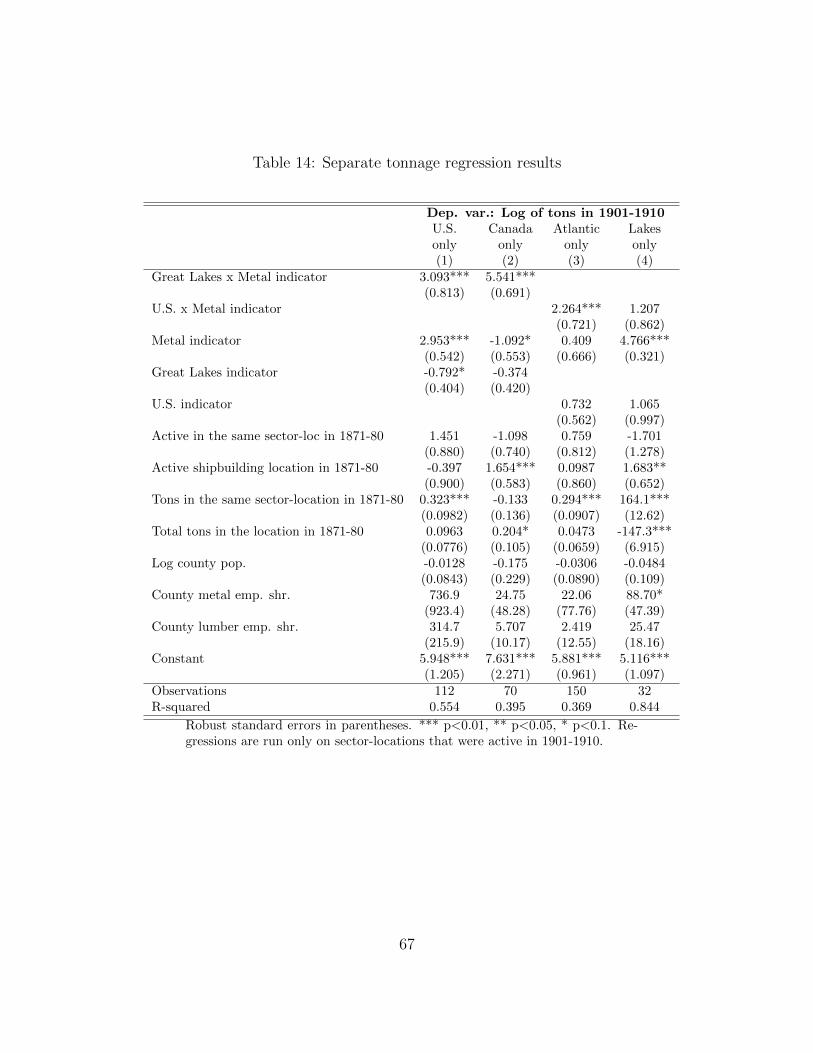
Table 14: Separate tonnage regression results

Dep. var.: Log of tons in 1901-1910U.S. Canada Atlantic Lakesonly only only only(1) (2) (3) (4)

Great Lakes x Metal indicator 3.093*** 5.541***(0.813) (0.691)

U.S. x Metal indicator 2.264*** 1.207(0.721) (0.862)

Metal indicator 2.953*** -1.092* 0.409 4.766***(0.542) (0.553) (0.666) (0.321)

Great Lakes indicator -0.792* -0.374(0.404) (0.420)

U.S. indicator 0.732 1.065(0.562) (0.997)

Active in the same sector-loc in 1871-80 1.451 -1.098 0.759 -1.701(0.880) (0.740) (0.812) (1.278)

Active shipbuilding location in 1871-80 -0.397 1.654*** 0.0987 1.683**(0.900) (0.583) (0.860) (0.652)

Tons in the same sector-location in 1871-80 0.323*** -0.133 0.294*** 164.1***(0.0982) (0.136) (0.0907) (12.62)

Total tons in the location in 1871-80 0.0963 0.204* 0.0473 -147.3***(0.0776) (0.105) (0.0659) (6.915)

Log county pop. -0.0128 -0.175 -0.0306 -0.0484(0.0843) (0.229) (0.0890) (0.109)

County metal emp. shr. 736.9 24.75 22.06 88.70*(923.4) (48.28) (77.76) (47.39)

County lumber emp. shr. 314.7 5.707 2.419 25.47(215.9) (10.17) (12.55) (18.16)

Constant 5.948*** 7.631*** 5.881*** 5.116***(1.205) (2.271) (0.961) (1.097)

Observations 112 70 150 32R-squared 0.554 0.395 0.369 0.844

Robust standard errors in parentheses. *** p<0.01, ** p<0.05, * p<0.1. Re-gressions are run only on sector-locations that were active in 1901-1910.

67

Table 15: Tonnage regression results in levels

Dep. var.: Log of tons in 1901-1910(1) (2) (3) (4) (5)

Great Lakes x Metal 150,758*** 126,277*** 126,778*** 120,751* 120,799*(47,672) (45,645) (47,040) (61,915) (62,938)

U.S. Coast x Metal 51,208*** 42,039*** 47,785**(16,453) (16,140) (22,439)

Metal indicator Yes Yes Yes Yes YesU.S. Coast ind. Yes Yes YesGreat Lakes ind. Yes Yes Yes Yes YesActivity in 1871 Yes Yes Yes YesTonnage in 1871 Yes Yes Yes YesNearby tons in 1871 YesCounty controls Yes YesInput prices Yes YesObservations 186 186 182 82 82R-squared 0.326 0.362 0.405 0.444 0.456

Robust standard errors in parentheses. *** p<0.01, ** p<0.05, * p<0.1. Regressions are run onlyon sector-locations that were active in 1901-1910. Column 2 includes controls for whether a locationis active in metal or wood shipbuilding in 1870 as well as separate variables for tonnage producedin metal or wood in 1870. Column 3 adds additional controls for metal or wood shipbuilding atother locations within 100km, county log population, the county employment share in metalworkingindustries, and the employment share in lumber. Note that the county data are not available forsome locations. Column 4 includes the controls in Column 2 together with the log price of pig ironand log lumber index price in the state. These are only available for a subset of U.S. states, so thenumber of observations drops substantially. Column 5 includes the controls in Column 4 togetherwith controls for county log population, the county employment share in metalworking industries,and the employment share in lumber.

68

A.15 Evidence on learning using cumulative production

Results examining the relationship between output in 1901-1910 and cumu-

lative previous production (since 1850) are shown in Table 16. Columns 1-2

present results looking at how cumulative production within a location prior

to 1901 was related to output in the location in 1901-1910. We can see that, in

metal shipbuilding previous cumulative production in the same sector-location

is related to current production with an elasticity ranging from 0.167-0.195.

No similar pattern appears in the more mature wood shipbuilding sector. Also,

the third row of estimated coefficients shows that after accounting for cumula-

tive production in the sector-location, there is some evidence that cumulative

production in the location overall was associated with greater output. Thus,

this provides some evidence that there may have been spillover benefits across

wood and metal production within a yard. One likely reason for this is that

they shared some common fixed capital and skilled labor inputs.

In Columns 3-4 I add in additional variables reflecting cumulative produc-

tion in other nearby (within 50km) locations. These provide evidence that

cumulative production in nearby locations was associated with increased out-

put in metal shipbuilding but not in wood shipbuilding. It is not clear why

we observe the difference between metal and wood shipbuilding here. One

potential reason may be that, because wood was a long-established sector,

knowledge had fully diffused so local learning no longer mattered. In Column

5 I look at the additional impact of cumulative production in locations from

50-100km away. Here I observe no evidence of an additional impact, which

suggests that any learning effects in metal shipbuilding were quite localized.

Finally, note that accounting for these local learning effects has little impact

on the own-location coefficients.

69

Table 16: Cumulative production results

DV: Log tons produced in a sector-location(1) (2) (3) (4) (5)

Log cumulative tons 0.195** 0.167** 0.192** 0.163** 0.157*by 1900 x Metal (0.0781) (0.0798) (0.0775) (0.0792) (0.0799)

Log cumulative tons 0.0909 0.0678 0.124 0.0937 0.0805by 1900 x Wood (0.0925) (0.0937) (0.0930) (0.0949) (0.0977)

Total log cum. tons 0.133 0.205** 0.0996 0.175* 0.187**in location by 1900 (0.0863) (0.0903) (0.0860) (0.0908) (0.0929)

Log cum. tons within 0.0993** 0.108** 0.107**50km x Metal (0.0498) (0.0488) (0.0511)

Log cum. tons within 0.00605 0.0324 0.0071450km x Wood (0.0323) (0.0333) (0.0446)

Log cum. tons within -0.014150-100km x Metal (0.0544)

Log cum. tons within 0.042650-100km x Wood (0.0481)

Additional controls:Active loc in 1870s Yes Yes YesActive sector-loc in 1870s Yes Yes YesCounty controls Yes Yes YesObservations 186 182 186 182 182R-squared 0.610 0.624 0.620 0.638 0.639

Robust standard errors in parentheses. *** p<0.01, ** p<0.05, * p<0.1. Regressions arerun only on sector-locations that were active in 1901-1910. All Columns include indicatorvariables for whether the sector is metal, whether the location was in the Great Lakes,whether the location was in the U.S., and the interaction of each of these variables with themetal sector indicator.

It is interesting to compare these results to the findings of previous work.

It is striking how similar the magnitude effects of cumulative output within

a location on current output are to estimates from Thompson (2001), who

estimates elasticities of around 0.2. Of course, these results are not strictly

comparable because he is able to control for input usage while I am not. In

general, we would expect this to cause his elasticity estimates to be smaller

than mine. However, Thompson is also looking at learning in the repeated

production of the same ship type, while my data includes a very wide variety

70

of types. If cumulative production has a larger effect within the same type

of ship then we should expect his estimates to be larger than mine. Thus, it

is not clear a priori whether to expect my estimates to be larger or smaller

than previous results, but the fact that they are fairly similar suggests that

my results are in the right ballpark.

It is also possible to compare the effect of spillovers across yards shown in

Table 16 to results on cross-yard spillovers from Thornton & Thompson (2001).

Looking at productivity in 25 Navy yards during WWII, they find that cross-

yard spillovers were limited. The results in Table 16 suggest that cross-yard

effects may be important, but that these are highly localized. The localized

nature of these effects may explain why Thornton & Thompson (2001) find

weak cross-yard spillover effects, since the yards in their analysis are often far

apart. The localized nature of these effects also provides a clue to the nature

of the underlying channels, a topic that I return to later.

71