Evolutionary Methods in Multi-Objective Evolutionary Methods in Multi-Objective OptimizationOptimization

- Why do they work ? -- Why do they work ? -

Lothar Thiele

Computer Engineering and Networks LaboratoryDept. of Information Technology and Electrical

EngineeringSwiss Federal Institute of Technology (ETH) Zurich

Computer EngineeringComputer Engineeringand Networks Laboratoryand Networks Laboratory

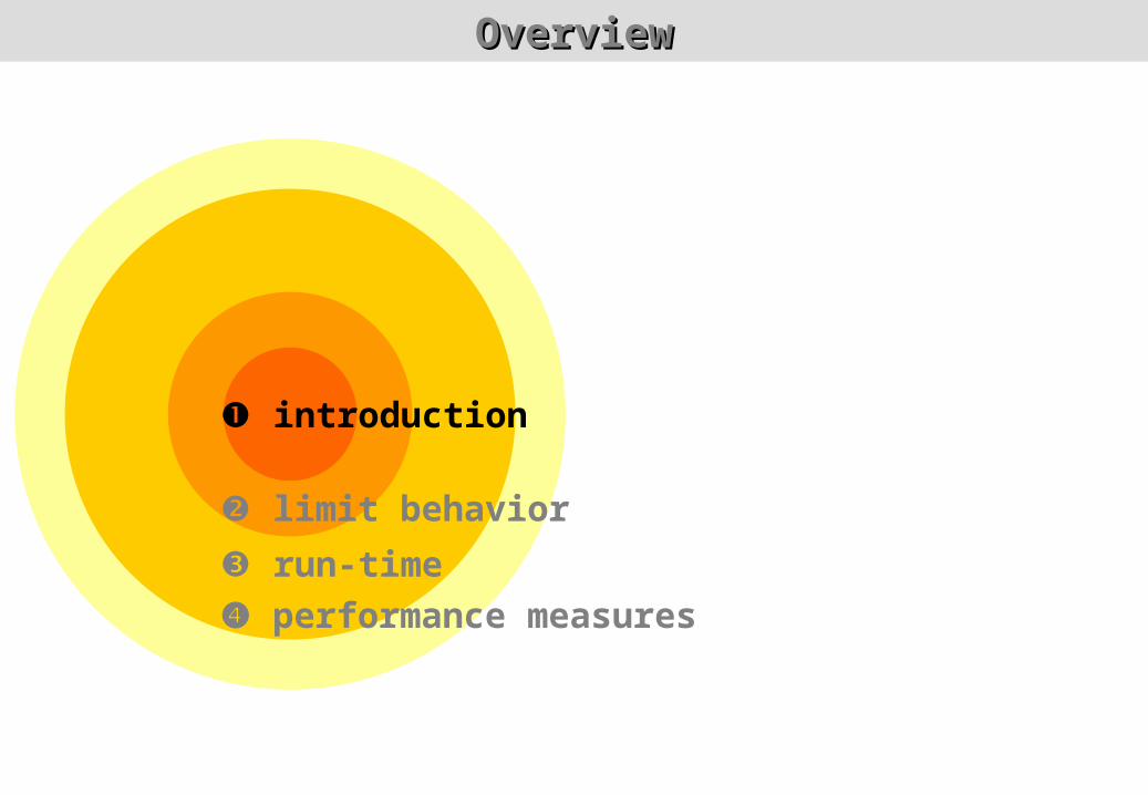
OverviewOverview

introduction

limit behavior

run-time performance measures

?

Black-Box OptimizationBlack-Box Optimization

Optimization Algorithm:

only allowed to evaluate f (direct search)

decision vector x

objective vector f(x)

objective function

(e.g. simulation model)

Issues in EMOIssues in EMO

y2

y1

Diversity

Convergence

How to maintain a diverse Pareto set approximation?

density estimation

How to prevent nondominated solutions from being lost?

environmental selection

How to guide the population towards the Pareto set?

fitness assignment

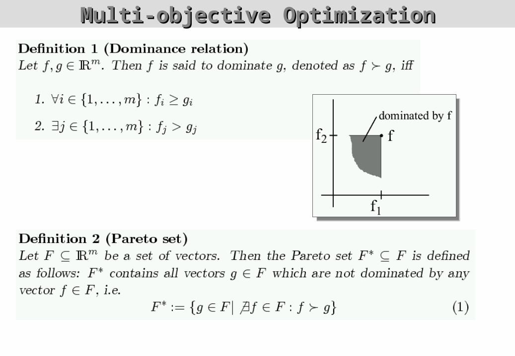
Multi-objective OptimizationMulti-objective Optimization

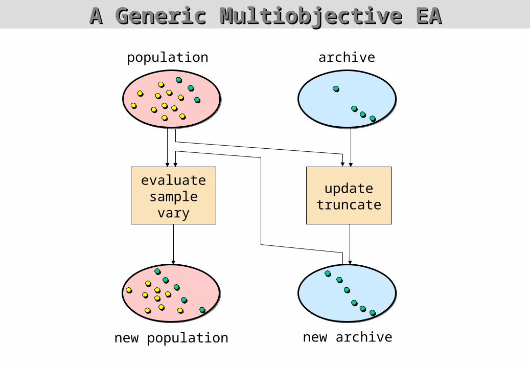
A Generic Multiobjective EAA Generic Multiobjective EA

archivepopulation

new population new archive

evaluatesample

vary

updatetruncate

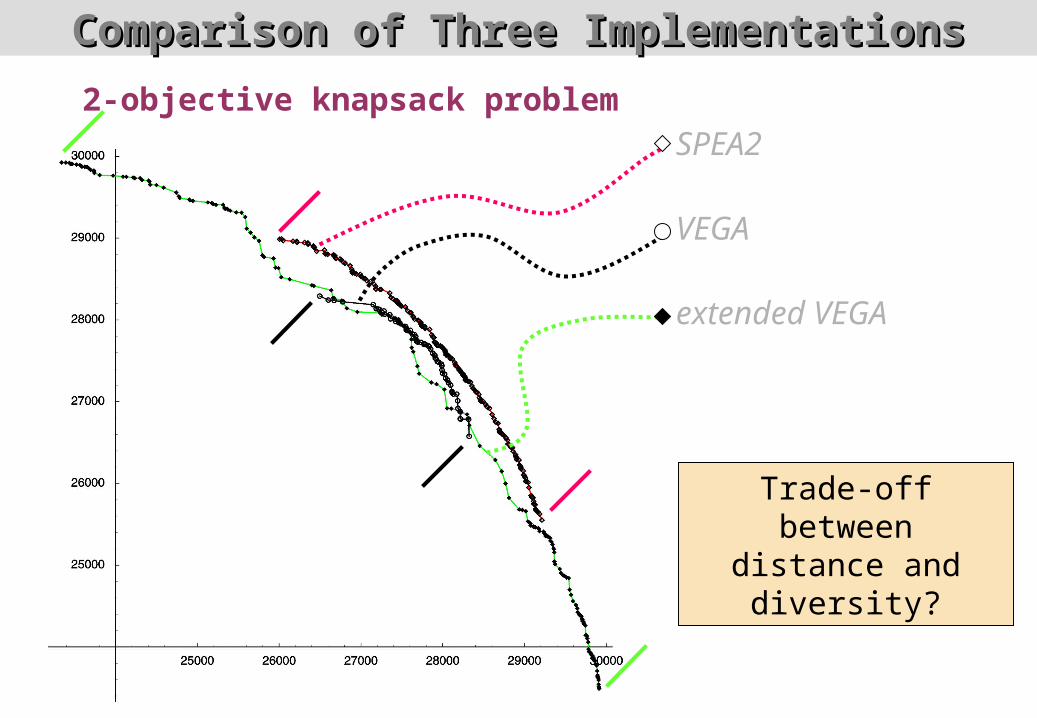
Comparison of Three ImplementationsComparison of Three Implementations

SPEA2

VEGA

extended VEGA

2-objective knapsack problem

Trade-off betweendistance and

diversity?

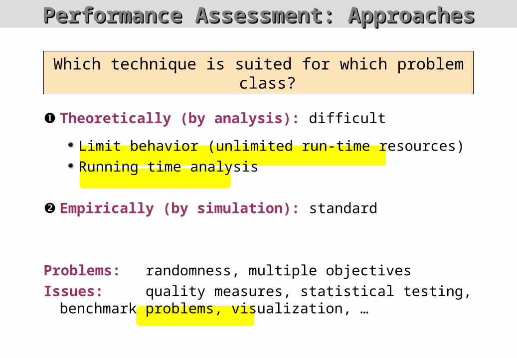
Performance Assessment: ApproachesPerformance Assessment: Approaches

Theoretically (by analysis): difficult

Limit behavior (unlimited run-time resources)Running time analysis

Empirically (by simulation): standard

Problems: randomness, multiple objectivesIssues: quality measures, statistical testing,

benchmark problems, visualization, …

Which technique is suited for which problem class?

OverviewOverview

introduction

limit behavior

run-time performance measures

Analysis: Main AspectsAnalysis: Main Aspects

Evolutionary algorithms are random search heuristics

Computation Time

(number of iterations)

Probability{Optimum found}

∞

1

1/2

Qualitative:

Limit behavior for t → ∞

Quantitative:

Expected Running Time E(T)

Algorithm A applied to Problem B

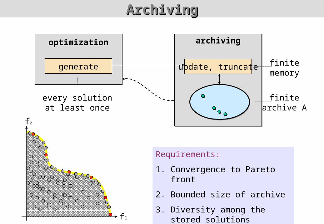
ArchivingArchiving

optimizationoptimization archivingarchiving

generate update, truncate finitememory

finitearchive A

every solutionat least once

f2

f1

Requirements:

1. Convergence to Pareto front

2. Bounded size of archive

3. Diversity among the stored solutions

Problem: DeteriorationProblem: Deterioration

f2

f1

f2

f1

t t+1

new solution

discarded

new solution

New solution accepted in t+1 is dominated by a solution found previously (and “lost” during the selection process)

bounded archive (size 3)

Goal: Maintain “good” front (distance + diversity)

But: Most archivingstrategies may forgetPareto-optimal

solutions…

Problem: DeteriorationProblem: Deterioration

NSGA-II

SPEA

Limit Behavior: Related WorkLimit Behavior: Related Work

Requirements for archive:

1. Convergence

2. Diversity

3. Bounded Size

(impractical)

“store all”

[Rudolph 98,00] [Veldhuizen 99]

“store one”

[Rudolph 98,00] [Hanne 99]

(not nice)

in this work

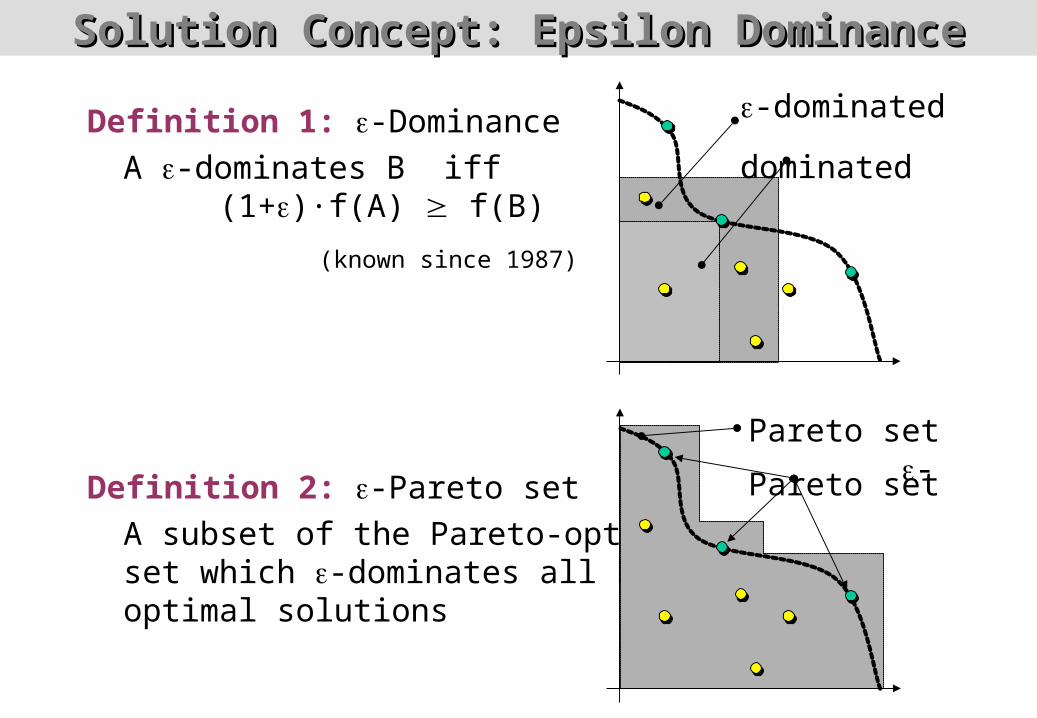
Solution Concept: Epsilon DominanceSolution Concept: Epsilon Dominance

Definition 1: -DominanceA -dominates B iff (1+)·f(A) f(B)

Definition 2: -Pareto setA subset of the Pareto-optimalset which -dominates all Pareto-optimal solutions

-dominated dominated

Pareto set -Pareto set

(known since 1987)

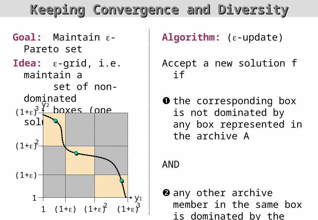
Keeping Convergence and DiversityKeeping Convergence and Diversity

Goal: Maintain -Pareto set

Idea: -grid, i.e. maintain a

set of non-dominated

boxes (one solution

per box)

Algorithm: (-update)

Accept a new solution f if

the corresponding box is not dominated by any box represented in the archive A

AND

any other archive member in the same box is dominated by the new solution

y2

y1

(1+)2

(1+)2 (1+)3

(1+)3

(1+)

(1+)

11

Correctness of Archiving MethodCorrectness of Archiving Method

Theorem:Let F = (f1, f2, f3, …) be an infinite sequence of objective vectorsone by one passed to the -update algorithm, and Ft the union ofthe first t objective vectors of F.

Then for any t > 0, the following holds: the archive A at time t contains an -Pareto front of Ft

the size of the archive A at time t is bounded by the term (K = “maximum objective value”, m = “number of objectives”)

1

)1log(

log

mK

Sketch of Proof:

3 possible failures for At not being an -Pareto set of Ft (indirect proof)at time k t a necessary solution was missedat time k t a necessary solution was expelledAt contains an f Pareto set of Ft

Number of total boxes in objective space:Maximal one solution per box acceptedPartition into chains of boxes

Correctness of Archiving MethodCorrectness of Archiving Method

mK

)1log(

log

1

)1log(

log

mK

)1log(

log

K

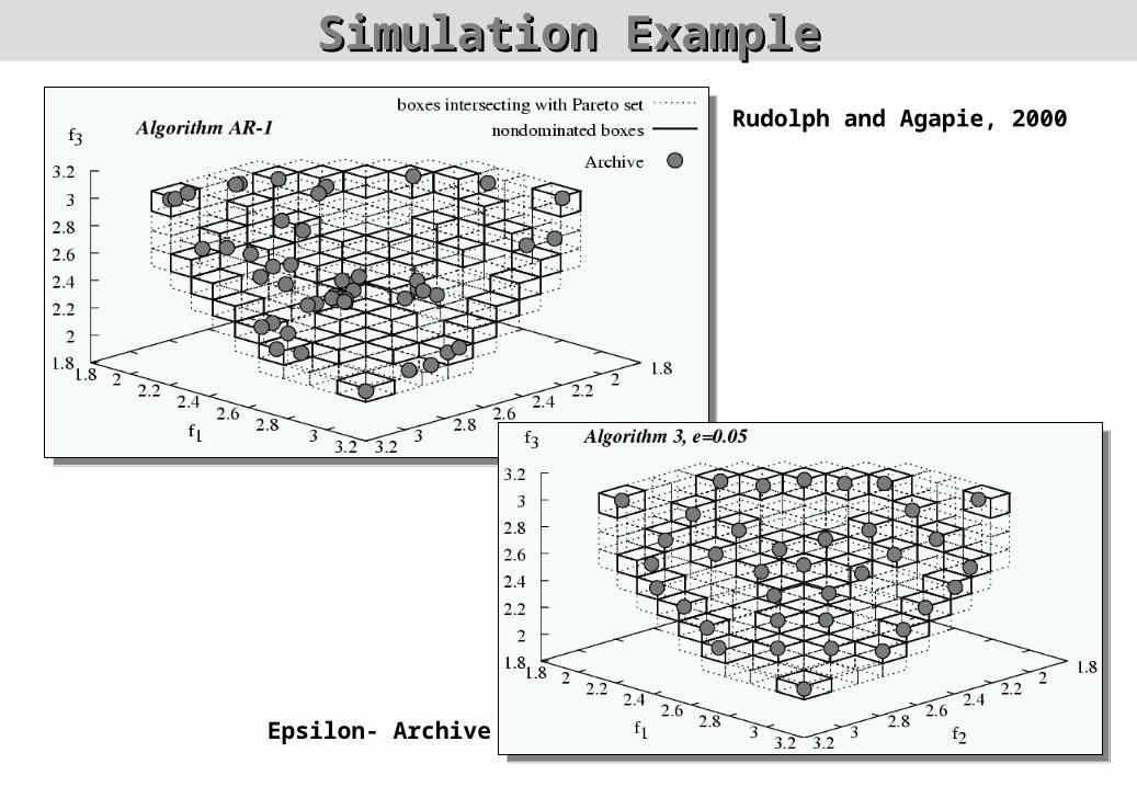
Simulation ExampleSimulation Example

Rudolph and Agapie, 2000

Epsilon- Archive

OverviewOverview

introduction

limit behavior

run-time performance measures

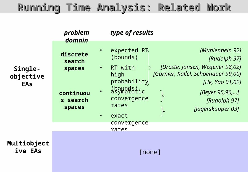
Running Time Analysis: Related WorkRunning Time Analysis: Related Work

Single-objective EAs

Multiobjective EAs

discrete search spaces

continuous search spaces

problem domain type of results

• expected RT (bounds)

• RT with high probability (bounds)

[Mühlenbein 92]

[Rudolph 97]

[Droste, Jansen, Wegener 98,02][Garnier, Kallel, Schoenauer 99,00]

[He, Yao 01,02]

• asymptotic convergence rates

• exact convergence rates

[Beyer 95,96,…]

[Rudolph 97]

[Jagerskupper 03]

[none]

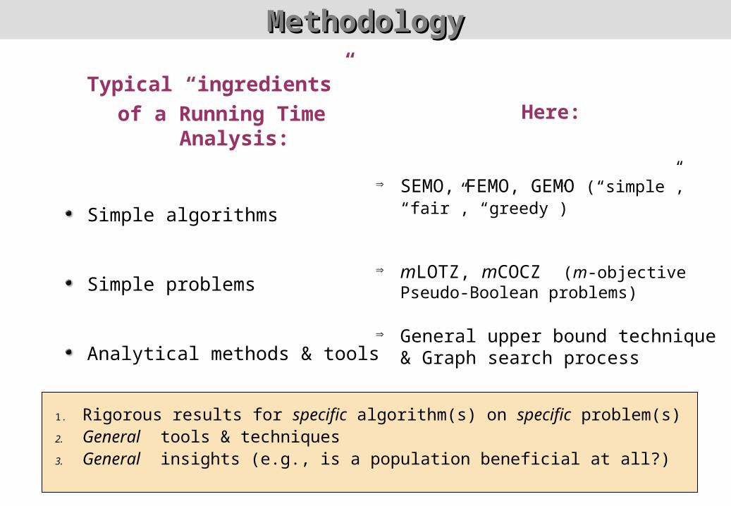
MethodologyMethodology

Typical “ingredients” of a Running Time

Analysis:

Simple algorithms

Simple problems

Analytical methods & tools

Here:

SEMO, FEMO, GEMO (“simple”, “fair”, “greedy”)

mLOTZ, mCOCZ (m-objective Pseudo-Boolean problems)

General upper bound technique & Graph search process

1. Rigorous results for specific algorithm(s) on specific problem(s)2. General tools & techniques 3. General insights (e.g., is a population beneficial at all?)

Three Simple Multiobjective EAsThree Simple Multiobjective EAs

selectindividual

from population

insertinto population

if not dominated

removedominatedfrom population

fliprandomly

chosen bit

Variant 1: SEMO

Each individual in thepopulation is selected

with the same probability(uniform selection)

Variant 2: FEMO

Select individual withminimum number of

mutation trials (fair selection)

Variant 3: GEMO

Priority of convergenceif there is progress (greedy selection)

SEMOSEMO

population Ppopulation P

x

x’

uniform selection

single pointmutation

include, if not dominated

remove dominated and duplicated

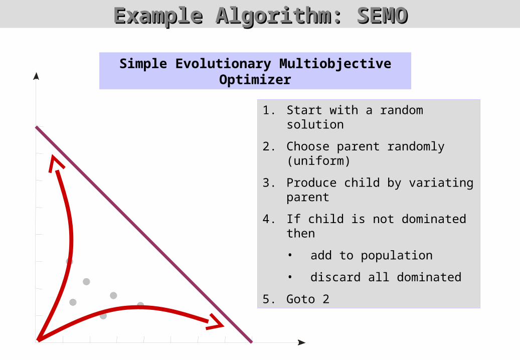
Example Algorithm: SEMOExample Algorithm: SEMO

1. Start with a random solution

2. Choose parent randomly (uniform)

3. Produce child by variating parent

4. If child is not dominated then

• add to population

• discard all dominated

5. Goto 2

Simple Evolutionary Multiobjective Optimizer

Run-Time Analysis: ScenarioRun-Time Analysis: Scenario

Problem:leading ones, trailing zeros (LOTZ)

Variation:single point mutation

one bit per individual

1 1 0 1 0 0 0

1 1 1 0 0 0

1 1 1 0 0 01

0

The Good NewsThe Good News

SEMO behaves like a single-objective EA until the Pareto sethas been reached...

y2

y1

trailing 0s

leading 1s

Phase 1:only onesolution storedin the archive

Phase 2:only Pareto-optimalsolutions storedin the archive

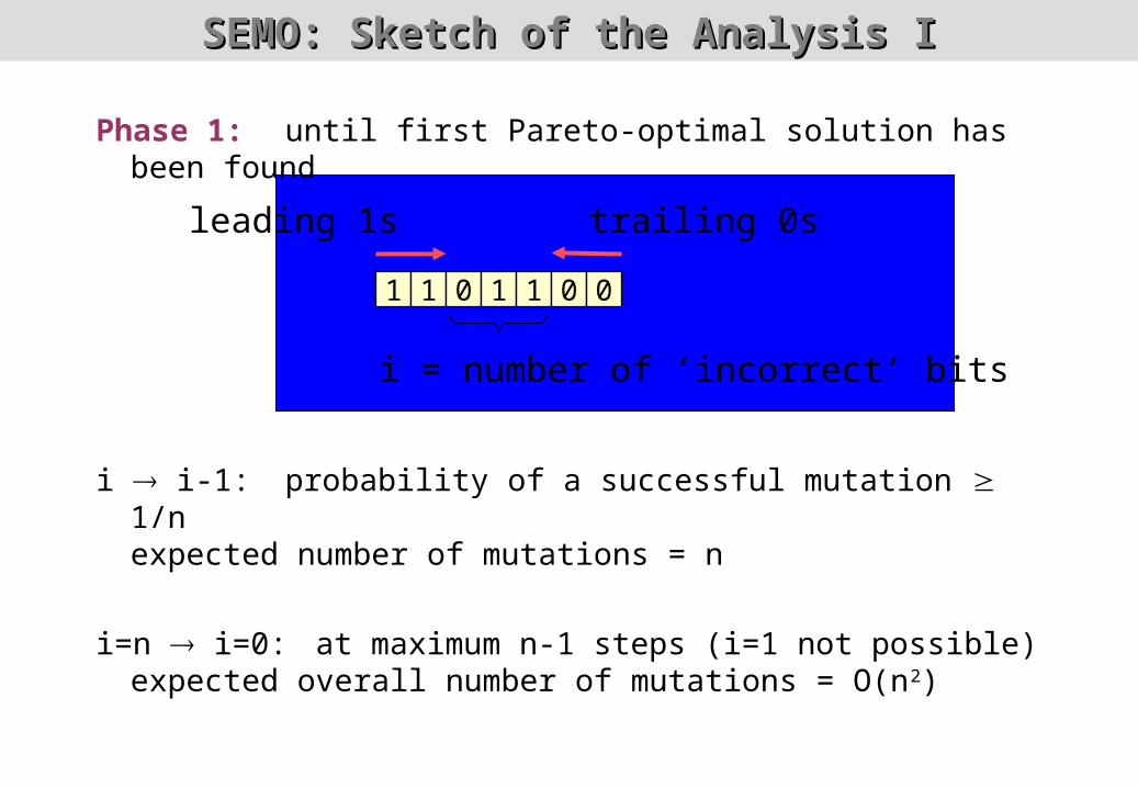
SEMO: Sketch of the Analysis ISEMO: Sketch of the Analysis I

Phase 1: until first Pareto-optimal solution has been found

i i-1: probability of a successful mutation 1/nexpected number of mutations = n

i=n i=0: at maximum n-1 steps (i=1 not possible)expected overall number of mutations =

O(n2)

1 1 0 1 1 0 0

leading 1s trailing 0s

i = number of ‘incorrect’ bits

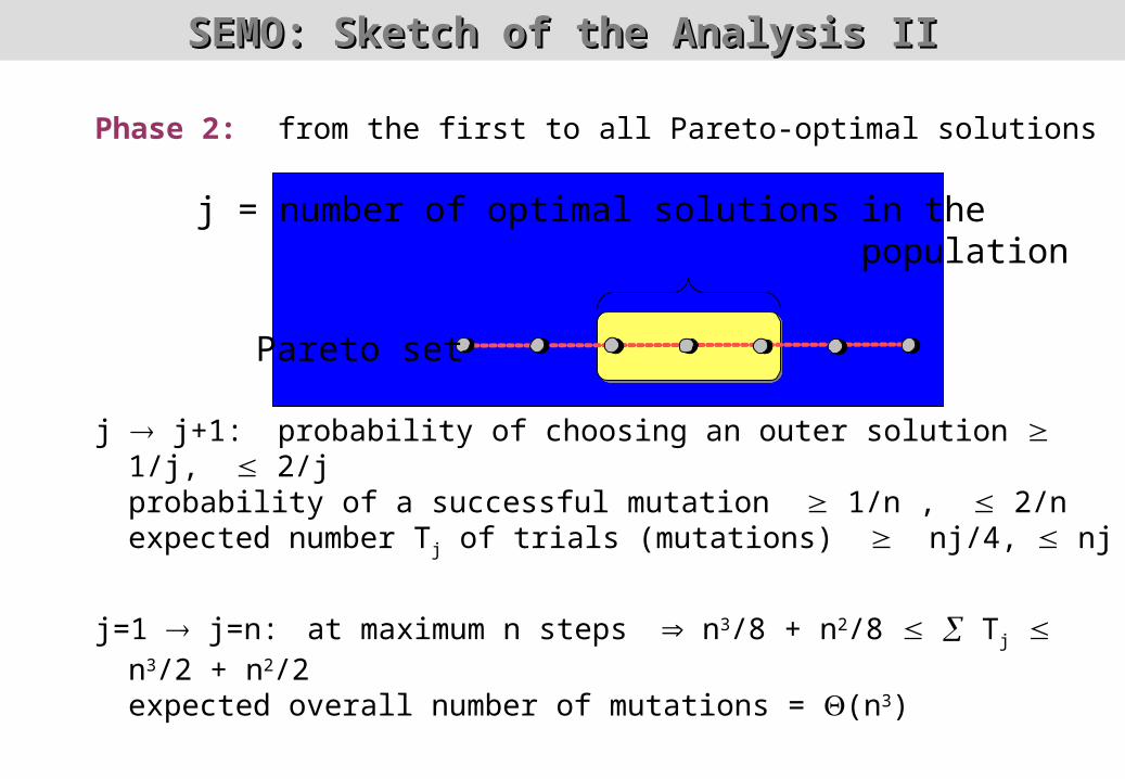
SEMO: Sketch of the Analysis IISEMO: Sketch of the Analysis II

Phase 2: from the first to all Pareto-optimal solutions

j j+1: probability of choosing an outer solution 1/j, 2/jprobability of a successful mutation 1/n , 2/nexpected number Tj of trials (mutations) nj/4,

nj

j=1 j=n: at maximum n steps n3/8 + n2/8 Tj n3/2 + n2/2

expected overall number of mutations = (n3)

Pareto set

j = number of optimal solutions in the population

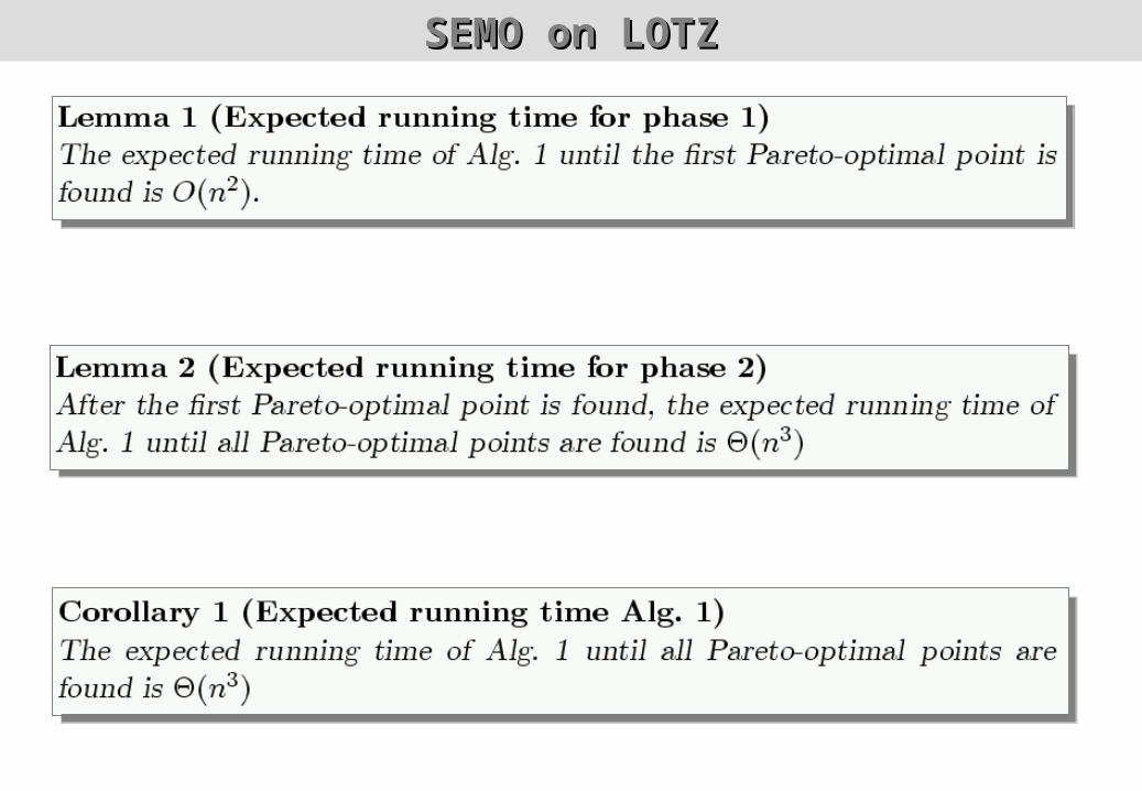
SEMO on LOTZSEMO on LOTZ

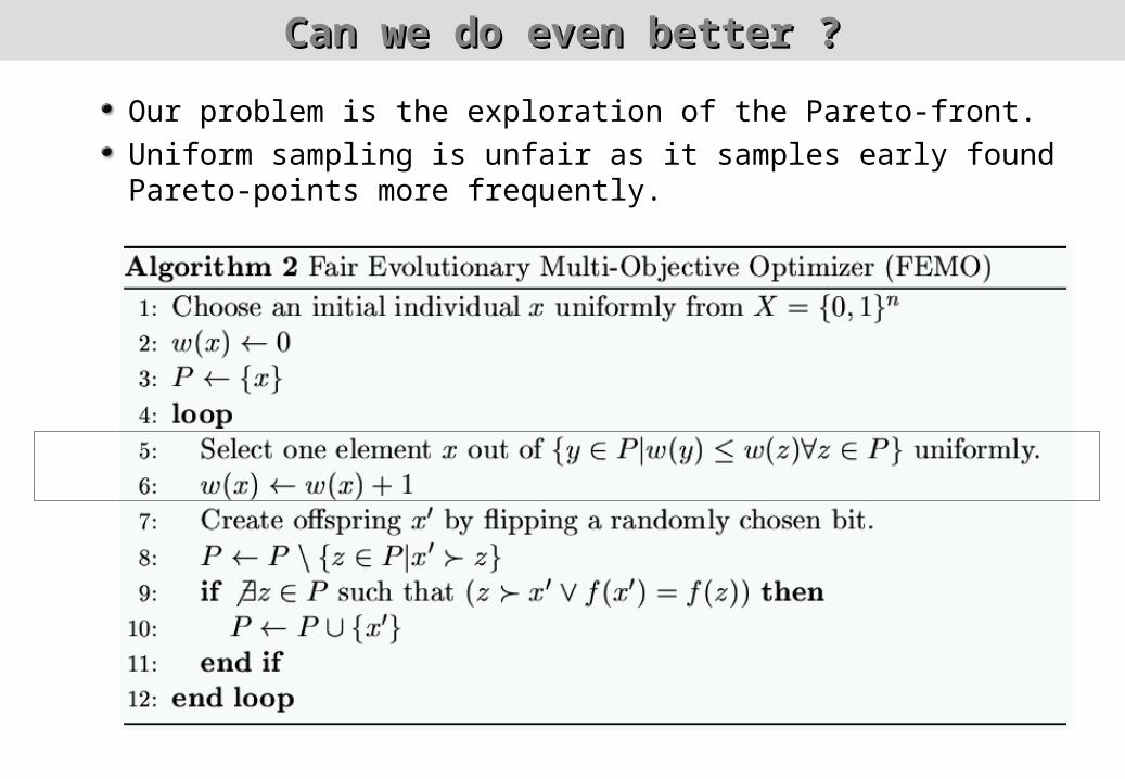
Can we do even better ?Can we do even better ?

Our problem is the exploration of the Pareto-front.Uniform sampling is unfair as it samples early found Pareto-points more frequently.

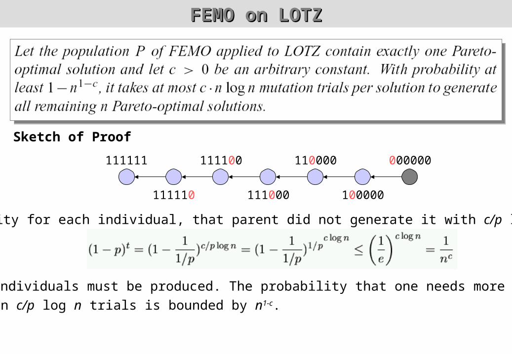
FEMO on LOTZFEMO on LOTZ

Sketch of Proof

000000

100000

110000

111000

111100

111110

111111

Probability for each individual, that parent did not generate it with c/p log n trials:

n individuals must be produced. The probability that one needs morethan c/p log n trials is bounded by n1-c.

FEMO on LOTZFEMO on LOTZ

Single objective (1+1) EA with multistart strategy (epsilon-constraint method) has running time (n3).

EMO algorithm with fair sampling has running time (n2 log(n)).

Generalization: Randomized Graph SearchGeneralization: Randomized Graph Search

Pareto front can be modeled as a graph

Edges correspond to mutations

Edge weights are mutation probabilities

How long does it take to explore the whole graph?

How should we select the “parents”?

Randomized Graph SearchRandomized Graph Search

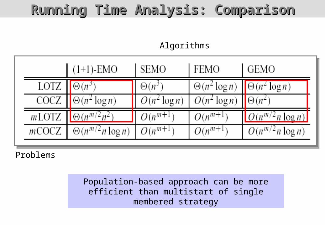
Running Time Analysis: ComparisonRunning Time Analysis: Comparison

Algorithms

Problems

Population-based approach can be more efficient than multistart of single membered strategy

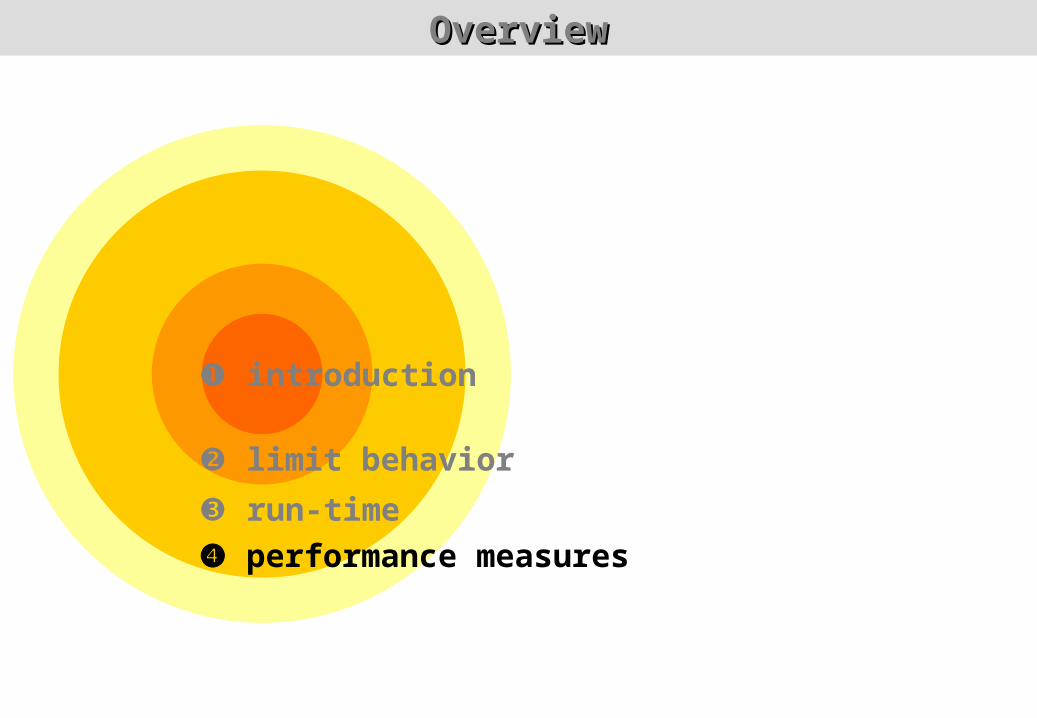
OverviewOverview

introduction

limit behavior

run-time performance measures

Performance Assessment: ApproachesPerformance Assessment: Approaches

Theoretically (by analysis): difficult

Limit behavior (unlimited run-time resources)Running time analysis

Empirically (by simulation): standard

Problems: randomness, multiple objectivesIssues: quality measures, statistical testing,

benchmark problems, visualization, …

Which technique is suited for which problem class?

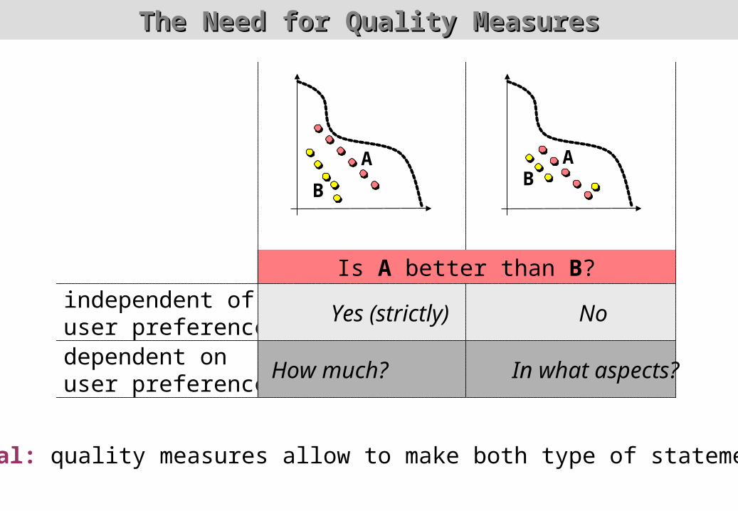
The Need for Quality MeasuresThe Need for Quality Measures

A

B

AB

independent ofuser preferences

Yes (strictly) No

dependent onuser preferences

How much? In what aspects?

Is A better than B?

Ideal: quality measures allow to make both type of statements

weakly dominates = not worse in all

objectives sets not equal

dominates= better in at least one

objective

strictly dominates= better in all objectives

is incomparable to= neither set weakly better

A

B

Independent of User Preferences Independent of User Preferences

C

D

A B

C D

Pareto set approximation (algorithm outcome) = set of incomparable

solutions

= set of all Pareto set approximations

A C

B C

Dependent on User PreferencesDependent on User Preferences

Goal: Quality measures compare two Pareto set approximations A and B.

A

B

hypervolume 432.34 420.13distance 0.3308 0.4532diversity 0.3637 0.3463spread 0.3622 0.3601cardinality 6 5

A B

“A better”

application ofquality measures

(here: unary)

comparison andinterpretation of

quality values

Quality Measures: ExamplesQuality Measures: ExamplesUnary

Hypervolume measureBinary

Coverage measure

performance

cheapness

S(A)A

performance

cheapness

B

A

[Zitzler, Thiele: 1999]

S(A) = 60%C(A,B) = 25%C(B,A) = 75%

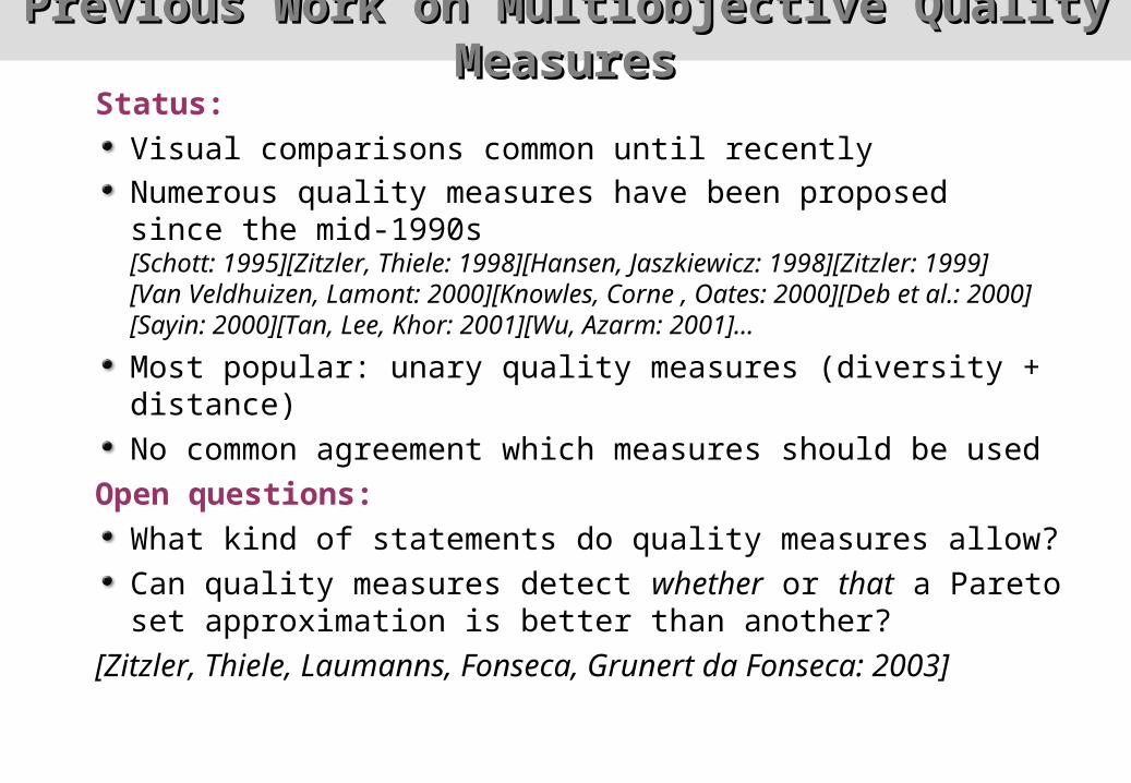
Previous Work on Multiobjective Quality Previous Work on Multiobjective Quality MeasuresMeasures

Status:Visual comparisons common until recentlyNumerous quality measures have been proposedsince the mid-1990s[Schott: 1995][Zitzler, Thiele: 1998][Hansen, Jaszkiewicz: 1998][Zitzler: 1999][Van Veldhuizen, Lamont: 2000][Knowles, Corne , Oates: 2000][Deb et al.: 2000] [Sayin: 2000][Tan, Lee, Khor: 2001][Wu, Azarm: 2001]…

Most popular: unary quality measures (diversity + distance)No common agreement which measures should be used

Open questions:What kind of statements do quality measures allow?Can quality measures detect whether or that a Pareto set approximation is better than another?

[Zitzler, Thiele, Laumanns, Fonseca, Grunert da Fonseca: 2003]

Comparison Methods and Dominance Comparison Methods and Dominance RelationsRelations

Compatibility of a comparison method C:

C yields true A is (weakly, strictly) better than B

(C detects that A is (weakly, strictly) better than B)

Completeness of a comparison method C:

A is (weakly, strictly) better than B C yields true

Ideal: compatibility and completeness, i.e.,

A is (weakly, strictly) better than B C yields true

(C detects whether A is (weakly, strictly) better than B)

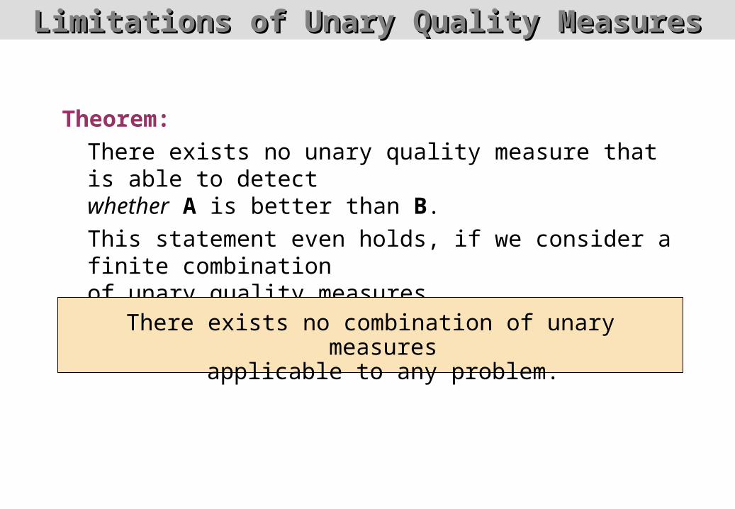
Limitations of Unary Quality MeasuresLimitations of Unary Quality Measures

Theorem:There exists no unary quality measure that is able to detectwhether A is better than B.This statement even holds, if we consider a finite combinationof unary quality measures.There exists no combination of unary measures

applicable to any problem.

Power of Unary Quality IndicatorsPower of Unary Quality Indicators

strictly dominates doesn’t weakly dominate doesn’t dominate weakly dominates

Quality Measures: ResultsQuality Measures: Results

There is no combination of unary quality measures such that

S is better than T in all measures is equivalent to S dominates T

ST

application ofquality measures

Basic question: Can we say on the basis of the quality measures

whether or that an algorithm outperforms another? hypervolume 432.34 420.13

distance 0.3308 0.4532diversity 0.3637 0.3463spread 0.3622 0.3601cardinality 6 5

S T

Unary quality measures usually do not tell thatS dominates T; at maximum that S does not

dominate T[Zitzler et al.: 2002]

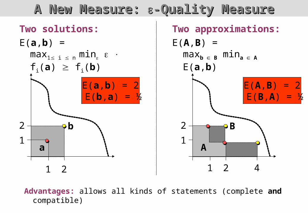
A New Measure: A New Measure: -Quality Measure-Quality Measure

Two solutions: E(a,b) =

max1 i n min fi(a) fi(b)

1 2 4

A

B2

1

E(A,B) = 2 E(B,A) = ½

Two approximations:E(A,B) =

maxb B mina A E(a,b)

a

b2

1

E(a,b) = 2 E(b,a) = ½

1 2

Advantages: allows all kinds of statements (complete and compatible)

Selected ContributionsSelected Contributions

Algorithms:° Improved techniques [Zitzler, Thiele: IEEE TEC1999]

[Zitzler, Teich, Bhattacharyya: CEC2000][Zitzler, Laumanns, Thiele:

EUROGEN2001]° Unified model [Laumanns, Zitzler, Thiele: CEC2000]

[Laumanns, Zitzler, Thiele: EMO2001]° Test problems [Zitzler, Thiele: PPSN 1998, IEEE TEC 1999]

[Deb, Thiele, Laumanns, Zitzler: GECCO2002]

Theory:° Convergence/diversity [Laumanns, Thiele, Deb, Zitzler:

GECCO2002][Laumanns, Thiele, Zitzler, Welzl, Deb:

PPSN-VII]° Performance measure [Zitzler, Thiele: IEEE TEC1999]

[Zitzler, Deb, Thiele: EC Journal 2000][Zitzler et al.: GECCO2002]

How to apply (evolutionary) optimization algorithms tolarge-scale multiobjective optimization problems?