Evolution of the Danish population from 1835 to 2000 · Danish population statistics, which embody...
125
Evolution of the Danish Population from 1835 to 2000
Transcript of Evolution of the Danish population from 1835 to 2000 · Danish population statistics, which embody...

Evolution of the Danish Populationfrom 1835 to 2000


Evolution of the Danish Populationfrom 1835 to 2000
Kirill F. Andreev
Monographs on Population Aging, 9.
Odense University Press

Evolution of the Danish Population
from 1835 to 2000
© Kirill F. Andreev and University Press of Southern Denmark, 2002
Printed by Special-Trykkeriet Viborg a-s, Denmark
Cover illustration: Herbs growing on the mountain of the two lovers.
Paper-cut by Sonia Brandes.
ISBN 87-7838-716-7
ISSN 0909-119X
Odense University Press
Campusvej 55
DK-5230 Odense M
Phone +45 66 15 79 99 - Fax +45 66 15 81 26
E-mail: [email protected]
Internet bookstore: www.universitypress.dk

Table of contents
Table of contents ........................................................................................................... 5List of tables .................................................................................................................. 6List of figures ................................................................................................................ 7Author............................................................................................................................ 8Acknowledgements ....................................................................................................... 91. Introduction ............................................................................................................. 112. Construction of the Danish mortality database....................................................... 13
2.1 Introduction ..................................................................................................... 132.2 Danish demographic statistics......................................................................... 132.3 Database structure ........................................................................................... 162.4 Original data .................................................................................................... 18
2.4.1 Population.................................................................................................. 182.4.2 Deaths ........................................................................................................ 18
2.5 Construction of the database ........................................................................... 192.5.1 Deaths ........................................................................................................ 19
Age zero........................................................................................................... 22Ages 100+........................................................................................................ 22Distribution of deaths by Lexis triangles........................................................ 23
2.5.2 Population.................................................................................................. 24Extinct cohort population................................................................................ 28Population at exact age.................................................................................... 30
3. A descriptive analysis of the evolution of the Danish population with focus on mortality ........................................................................................... 31
3.1 Danish population changes over the period 1835–2000 ................................ 313.2 The Danish mortality evolution ...................................................................... 38
3.2.1 Life expectancy at birth.............................................................................. 383.2.2 Period survivorship .................................................................................... 403.2.3 Mortality..................................................................................................... 413.2.4 Rates of mortality changes over time ....................................................... 503.2.5 Sex ratio of mortality ................................................................................. 523.2.6 Compression of mortality .......................................................................... 55
4. A comparison of mortality in Denmark and other developed countries ................ 634.1 Introduction ..................................................................................................... 634.2 Denmark to Sweden ........................................................................................ 63

4.3 Denmark to Norway ........................................................................................ 664.4 Denmark to Finland......................................................................................... 694.5 Denmark to the Netherlands............................................................................ 714.6 Denmark to Austria ......................................................................................... 714.7 Denmark to France .......................................................................................... 744.8 Denmark to England and Wales...................................................................... 764.9 Denmark to Japan............................................................................................ 784.10 Denmark to Canada......................................................................................... 804.11 Concluding notes............................................................................................. 82
5. Cause-specific mortality.......................................................................................... 875.1 An analysis of cause-specific mortality .......................................................... 875.2 Time trends in cause-specific mortality.......................................................... 94
6. Conclusions and further research.......................................................................... 1056.1 Main results ................................................................................................... 1056.2 Further research............................................................................................. 107
References ................................................................................................................. 111Appendix ................................................................................................................... 115Odense Monographs on Population Aging............................................................... 124
List of tables
2.1 The death distribution within the age group 95–99 and inthe year 1916 and 1921–1940 ........................................................................... 21
2.2 The number of deaths above age 100................................................................ 233.1 Annual gains in Danish life expectancy in the selected periods....................... 393.2 Life expectancy in the beginning of the 20th century ...................................... 503.3 Proportions of the life table deaths in Denmark ............................................... 585.1 Decomposition of excess Danish mortality by causes of death
for the period 1985–1993 .................................................................................. 905.2 Decomposition of excess Danish mortality by aggregated
causes of death for the period 1985–1993 ........................................................ 94

List of figures
2.1 Illustration of the Danish database structure with Lexis diagram.................. 172.2 Deviation between the original and the redistributed populations................. 293.1 Changes in the Danish population from 1835 till 2000.................................. 323.2 Changes in the age structure of the Danish population .................................. 323.3 Danish population distribution........................................................................ 343.4 Ratio of the Danish population distribution to the average levels
in 1835–1920................................................................................................... 353.5 Cumulative growth rate of the Danish population.......................................... 373.6 Danish life expectancy at birth........................................................................ 393.7 Danish survivorship by single calendar year .................................................. 423.8 Danish death rates ........................................................................................... 433.9 Rate of Danish mortality changes over time................................................... 543.10 Sex ratio of Danish mortality .......................................................................... 553.11 Danish life table death distribution................................................................. 573.12 Entropy of Danish life table death distribution .............................................. 604.1 Ratio of death rates, Denmark to Sweden....................................................... 654.2 Ratio of death rates, Denmark to Norway ...................................................... 684.3 Ratio of death rates, Denmark to Finland ....................................................... 704.4 Ratio of death rates, Denmark to the Netherlands.......................................... 724.5 Ratio of death rates, Denmark to Austria........................................................ 734.6 Ratio of death rates, Denmark to France ........................................................ 754.7 Ratio of death rates, Denmark to England and Wales.................................... 774.8 Ratio of death rates, Denmark to Japan .......................................................... 794.9 Ratio of death rates, Denmark to Canada ....................................................... 814.10 The highest death rates in Denmark compared with other countries ............. 854.11 The lowest death rates in Denmark compared with other countries .............. 855.1(a) Disadvantageous trends in Danish cause-specific mortality. Males.. ............ 965.1(b) Disadvantageous trends in Danish cause-specific mortality. Females......... 1006.1 Annual consumption of alcohol (population aged 15 and over) .................. 1096.2 Annual consumption of tobacco (population aged 15 and over) ................. 109
Note that most of the Lexis maps are available in color on the accompanying CD-ROM.

Author
Kirill F. AndreevDepartment of Community Health & EpidemiologyAbramsky HallQueen’s UniversityKingston, OntarioCanada K7L 3N6Home page: http://post.queensu.ca/~andreevk/E-mail: [email protected]: [email protected]

Acknowledgements
I am grateful to James W. Vaupel and Bernard Jeune for promoting my work on thisproject. I wish also to thank Anatoli Yashin, Väinö Kannisto, Roger Thatcher, ShiroHoriuchi, Hans Chr. Johansen, Vladimir Shkolnikov, Ivan Iachine, MichaelBubenheim for numerous discussions of demographic problems; John Wilmoth,Hans Lundström, Axel Skytthe, Dorthe Larsen, Otto Andersen, Michael Væth,Jacques Vallin, Thomas Burch, Ewa Tabeau, Frans Willikens, Jens-Kristian Borgan,Nico Keilman, Kirsten Enger Dybendal, Timo Nikander, Alexia Fürnkranz-Prskawetz, Alexander Hanika, Steve Smallwood and Dimiter Philipov for makingavailable mortality data.
I am grateful to Kirsten M. Gauthier for help with book layout and SigridGellers-Barkmann for help with data acquisition and preparation. I also extend mythanks to the entire staff of the Max Planck Institute for Demographic Research andof the University of Southern Denmark for their overall support of this project. Theproject has been completed at Queen's University, Canada with kindly support ofSamuel Shortt and Boris Sobolev.
This research was supported in part by grants from the U.S. National Instituteon Aging (P01-08761), the Danish Research Councils and the Max Planck Institutefor Demographic Research.


11
1. Introduction
We have the 17th-century parish registrars and their far-sighted collection ofstatistical data – which has been carried on to the present day by governmentstatisticians – to thank for the fact that we are now in a position to study differentaspects of the human life span. One of the major topics in demographic research isthe continuing mortality decline in European countries. Although many researchershave been studying the mortality transition of the last two centuries in Europe, "ourunderstanding of historical mortality patterns, and of their causes and implications, isstill in its infancy" (Schofield and Reher, 1991).
Research in this area is usually hampered by the lack of reliable long-termmortality series. Danish population statistics, which embody an enormous amount ofrelevant data extending well back into the seventieth century, are an importantexception. One of the outstanding features of the Danish statistics is that one can usethem to reconstruct the mortality evolution by a single age, year and cohort. Bystudying age-specific and cohort-specific mortality trends rather than by simplyusing the crude mortality indicators, deeper insights into the nature of mortalitydevelopment can be gained.
Chapter 2 is devoted to the authoritative account of the construction of theDanish mortality database. In this chapter, I bring together all sources of originalinformation on Danish population and provide a brief description of the history ofDanish population statistics. Estimation of Danish death rates over age and time cannot be carried out by solely using the official published population data. Forexample, in the 19th century population estimates for years between censuses are notavailable and deaths are aggregated into 5-year age groups. Moreover, populationestimates at the highest ages are not always given up to the last age attained ratherthey are published as open age aggregates, i.e. 90 and over. Estimation of death ratescan still be accomplished if missing population estimates are produced andadjustment of original data to the desired level of detail is carried out by specialmethods. A description of such methods is also included in Chapter 2.
The subject of the next chapter is a descriptive analysis of the evolution of theDanish population since 1835. The chapter includes an investigation of changes inthe Danish population structure with an emphasis on population aging, an analysis oftrends in death rates over age and time, an exploration of rates of mortality decline,an examination of compression of mortality and an investigation of male-femaledifferences in survival. Most of the findings are provided in great details and the

12
results are presented with the help of the Lexis map techniques (Caselli et al., 1985;Caselli et al., 1987; Vaupel et al., 1998).
Chapter 4 includes the results of a comparison of Danish mortality with deathrates in other countries. Nine countries (Sweden, Norway, Finland, the Netherlands,France, England and Wales, Austria, Canada and Japan) have been selected forcomparison with Denmark. All of them have a long history of reliable populationstatistics and comparable statistical resources. Country specific differences insurvival are investigated with the help of mortality ratio surfaces, which areestimated by the single calendar year and single year of age, for all ages from 0 to 99and for all years where data were available. The analysis clearly revealed age-specific differences in Danish survival and exposed their dynamics over time. Tworemarkable findings of this analysis are the unfavorable development in death ratesof middle-aged and the excess of Danish mortality compared to other countries inrecent decades.
Understanding of the determinants of disadvantageous trends in Danishmortality can be significantly improved by the analysis of causes of deaths. Cause-specific mortality developments over the last three decades in Denmark, Sweden, theNetherlands and Japan have been investigated in Chapter 5. The analysis helped toreveal the causes of deaths, providing the most significant contributions to the excessof Danish mortality in recent years. The trends in the causes of deaths, which are ofconcern, are also reported and discussed.
The monograph is accompanied by a CD-ROM containing the electronicversion of the monograph itself, color and black/white Lexis maps included in themonograph, the trends of the analyzed causes of deaths and the animated graphs ofDanish population and mortality changes.
The value of the Danish mortality data is not limited by the analysis conductedin this monograph. The database includes both data on population and deaths andpermits an estimation of death rates over age, time and along the cohort lines. Forthese reasons, the database can be extremely useful for mortality and populationprojections; for the wide range of epidemiological studies in which the mortality ofthe Danish population as a whole is compared with the mortality in selected groupsof individuals (e.g., Christensen, K. et al., 1995); for studies on the influence ofdifferent genes on the human life span where dynamics of gene proportions over ageis analyzed (Yashin et al., 1998). In the last case, for example, estimation of relativerisks associated with a particular genotype requires mortality estimates for cohortsborn a hundred years ago and earlier.

13
2. Construction of the Danish mortality database
2.1 Introduction
Construction of the Danish mortality database described in this section, has theprimary goal of estimating death rates over age and time by single calendar year andby single year of age. Official statistical information necessary for such purpose isavailable only for recent decades. Proceeding to earlier years, requires theapplication of non-trivial methods for adaptation of death counts and the productionof intercensual population estimates. Section 2.2 provides a brief historical review ofDanish population statistics, which is an ultimate source of information underlyingthis project. Section 2.3 includes the necessary information about the databasestructure and its coverage. In section 2.4, I discuss the available raw data used fordatabase compilation and section 2.5 brings together the methods that have beenused for achieving the desired level of data completeness and aggregation.
2.2 Danish demographic statistics
The Danish population and vital statistics are rooted in the seventeenth century,when parish registers became compulsory. In this section, I list the demographicevents relevant to the present work in chronological order. The informationpresented here is based mostly on publications of Matthiessen (1970) andImpagliazzo (1984). Detailed information on early Danish parish registers can befound in Johansen (1998).
1645–1646 - parish registers of births, deaths and marriages maintained by the clergy
became compulsory by rescript. The territory of Denmark was covered only partiallyin the following few decades.
1735 - summary statistics of parish registers became available annually in the form
of a statistical publication called the “General Extract”.
1769, August 15th. First census. Census information was presented in summary
tables. The population was divided by sex, and age was reported by six groups forthe ages under 48 and by an open age class 48+. Marital status was recorded asmarried and non-married. Occupational status was divided into nine groups.Although the enumerated population was "de jure population", some temporarilyabsent persons, e.g. sailors, may have been omitted. Some military personnel werealso excluded from the enumeration for security reasons.
1775 - A prescribed schedule of vital statistics was introduced. Clergy used this
schedule to fill in deaths by sex and 10-year age groups, and births by sex and

14
legitimacy. Starting in 1783, the number of marriages was also included.
1787, July 1st. Second census. This census was similar to that of 1769, with the
exception that the names of the individuals were recorded as well.
1796 - The first statistical office (Tabelkontoret) was founded. This office conducted
the 1801 census. The office was abolished in 1819 in favor of the statisticalcommission (Tabelkommisionen).
1800 - Births reported by the clergy were divided into the categories live-births and
stillborn.
1801, February 1st. Third census. The population was enumerated by 10-year age
groups. Statistical reports of this census were published together with the reports ofthe 1834 census.
1829 - Introduction of the death certificate.
1834, February 18th. Fourth census. This is the first census conducted by the
Tabelkommisionen. The population was enumerated by 10-year age groups. Theresults of this census were published in the first statistical publication (Tabelværket,1st series, 1st volume).
1835 - The distribution of marriages by broad age groups was introduced. Deaths
became recorded by the following age groups: below 1 year, 1–2 years, 3–4 years, 5–9 years, etc. Such detailed death statistics made possible the calculation of reliablemortality estimates.
1840, February 1st. Fifth census. The population was recorded by five-year age
groups and by single age for ages under five. This is the first census in which thepopulation was tabulated by five-year age groups.
1845, February 1st. Sixth census.
1850 - The national statistical office was founded (Statens Statistiske Bureau, later
Det Statistiske Department, and presently Danmarks Statistik).
1850, February 1st. Seventh census.
1855, February 1st. Eighth census.
1860, February 1st. Ninth census. The birth distribution by age of mother was
introduced.
1864, Autumn. Sønderjylland (hertugdømmet Slesvig) became part of Germany.
About 55,000 people emigrated from this region in 1867–1900, the major part toAmerica and a smaller part to Denmark.
1870, February 1st. Tenth census. For the first time the population was reported by
single age. The island of Ærø became part of Denmark with the peace treaty of 30October 1864 and was included in the census statistics.

15
1877 - Birth certificates were required everywhere in Denmark.
1880, February 1st. Eleventh census.
1890, February 1st. Twelfth census.
1901, February 1st. Thirteenth census.
1906, February 1st. Fourteenth census.
1911, February 1st. Fifteenth census.
1911 - Individual data on birth, marriage and death were sent from clergy to the
national statistical office, thereby abolishing the former schedule of vital statistics.
1916, February 1st. Sixteenth census.
1920, June 15th - Sønderjylland (hertugdømmet Slesvig) became part of Denmark,
thereby increasing the total population by about 163,000 people (about 5.5%).
1921, February 1st. Seventeenth census.
1925, November 5th. Eighteenth census.
1930, November 5th. Nineteenth census.
1935, November 5th. Twentieth census. In this census, questionnaires were
distributed to all individuals.
1940, November 5th. Twenty-first census.
1945, June 15th. Twenty-second census.
1950, November 7th. Twenty-third census.
1955, October 1st. Twenty-fourth census.
1960, September 26th. Twenty-fifth census.
1965, September 27th. Twenty-sixth census.
1968 The Central Population Register (CPR) was established. The process of
registering statistical information became continuous. The establishment of the CPRled to the abolishment of the questionnaire-based census.
1970, November 9th. Twenty-seventh census. This is the last census, which used
questionnaires.
1976, January 1st. First CPR based census.
1981, January 1st. Second CPR based census.Information on vital statistics has been published in the Table Works (StatistiskTabelværker) since the year 1801. The first publication covers the period from 1801to 1833 and was published together with the 1801 and 1834 censuses. All otherpublications cover five-year periods. The population statistical report (BefolkningensBevægelser) has been published since 1931 on an annual basis. This publicationincludes annual estimates of Danish population and its change over single year dueto deaths, migration and births. To complete the review of Danish statistics, I have

16
reproduced the table of former publications of Danish statistics from BefolkningensBevægelser 1999 in the Appendix Table 1. The most recent publications, e.g.Befolkningens Bevægelser 1999, are available online and can be downloadedthrough Danmarks Statistik1 web site.
Two other sources of population statistics, which are important to mention,include the publication "Dødsårsagerne i Danmark" (Causes of Death in Denmark)issued by the Danish Ministry of Health (Sundhedsstyrelsen, www.sst.dk) and thepublication "Befolkningen i kommunerne pr. 1. Januar" (Population by provinces)published by the Danmarks Statistik.
2.3 Database structure
The right choice of database structure can substantially reduce both the cost of dataretrieval and the basic computational operations performed on the data. Based on myexperience the following database structure is suggested:
COHORT AGE POPULATION DEATHS TIMING YEAR
… Example of records … …1940 30 32,592 13 1 19701939 30 31,256 16 2 1970… … … … … …
As the data are collected by years, the database is kept sorted by YEAR, AGE andTIMING, and each year includes the same number of ages, and each age includestwo timings or Lexis triangles. The Lexis diagram shown in Fig 2.1 illustrates therationale for the proposed structure.
The database includes six fields and each record is used to store theinformation about one Lexis triangle (TIMING). Timing “1” corresponds to thetriangle BCD and the timing “2” to the triangle ABD. The column DEATHScontains the number of deaths in these Lexis triangles. For example, in the abovegiven table, 13 deaths occurred in the cohort z=1940, year y=1970 and age x=30.
The 16 deaths which occurred in the same year and age, but in the previous cohortz=1939, belong to timing 2 (triangle ABD). Consequently, the sum of the deaths in
timings 1 and 2 is the number of deaths occurred in the given year and age (rectangleABCD). The interpretation of numbers stored in the field POPULATION depends onthe timing number. If the timing is equal to one, the population at risk at exact age x
over period [y, y+1] is recorded, otherwise it is the population on January 1st year y
1 National statistical office of Denmark. Danmarks Statistik, Sejrøgade 11, 2100 København Ø. E-mail: [email protected]. Internet: www.dst.dk.

17
G
F
2
1
HE
A D
CB
z+1
z
z-1
Cohor
t
Year
Age
x+2
x+1
x
y+2y+1y
Nx,y
Nx,y~
Figure 2.1. Illustration of the Danish database structure with the Lexis diagram
aged [x, x+1] that is listed. In our example, the population numbers are depicted by
lines BC and BA on the Lexis diagram and equal to 32,592 and 31,256, respectively.The database structure presented here is not optimized for the size. The variablesYEAR, COHORT, AGE and TIMING are linearly dependent and we can compute,for examples, the YEAR variable as YEAR = COHORT + AGE + TIMING - 1. Inother words, one of these four variables can safely be omitted without any loss ofinformation, but given the importance of all fields and computational conveniences,they are kept in the database intentionally since this permits a significant reductionin the time of computations.
Data stored in such a format can be used for calculations of virtually anydemographic indicators: central death rates, period and cohort life tables, rates ofmortality changes in time or age directions, et cetera. In addition, the absolutenumbers of population estimates and deaths stored in the database permit us to teststatistical hypotheses and to construct confidence intervals for the computed values.More detailed discussion of the Lexis diagram can be found in Impagliazzo (1984)and Tabeau et al. (1994). In the latter report, the different observational planes usedby the national statistical offices are also discussed. The reader interested in the

18
historical aspects of the development of this diagram may refer to Vandeschrick(2001).
2.4 Original data
2.4.1 Population
Danish population data before 1906, are available only from censuses, which wereheld every five or ten years. The censuses held in 1801 and 1834, tabulate populationby ten-year age groups and those held between 1834 and 1870 by five-year agegroups. As of 1870, the population is tabulated by single-age groups, which makesthese censuses entirely suitable for our requirements as the population estimates areavailable with the necessary level of details. The major part of the work onpopulation estimates for the 19th century, therefore, is concentrated on reconstructingthe single-age distribution and computing population estimates for the periodsbetween censuses. All Danish censuses in the nineteenth century were datedFebruary 1st, with the only exception in 1834 (February 18th). The database formatrequires that the population estimates are for January 1st, therefore an additionalpopulation adjustment has to be made.
Starting in 1906, population estimates by single year of age are available fromDanmarks Statistik. They can be added directly to the database. For the years 1906–1940, the population at higher ages is given by the open age class 85+, leaving thesingle-age distribution unknown. In this case, the population can be estimatedindirectly by the extinct cohort method (Vincent, 1951). Some data uncertainties alsoexist during the period from 1932 to 1940, as the population estimates available forthese years were rounded off to hundreds. Appendix Table 2 summarizes theavailable raw population statistics.
2.4.2 Deaths
The information about the available data on deaths is included in the Appendix Table3. The period from 1943 to the present time does not require any additionalmanipulations – the death counts can be added directly to the database. For theperiod from 1921 to 1942, the data are available in the same degree of detail, withthe exception that deaths for ages above 100 were aggregated into the single-agegroup 100+. The deaths in this age group have to be separated by a single year ofage. The death counts recorded in this group are very small, and the influence of theseparation procedure on mortality estimates at lower ages is negligible.
The data become less abundant as we move back to the earlier years. In theperiod 1916–1920, the death counts are given by single year and age (see Fig. 2.1,

19
rectangle ABCD). Here the death counts have to be split between cohorts in somereasonable way.
In the period 1835–1915, the death counts are given only in five-year agegroups. These data have to be separated by a single year of age and afterwards by acohort to fit the database standard.
2.5 Construction of the database
2.5.1 Deaths
1921–1999Data on deaths available for these years fit the database structure entirely and wereadded directly to the database, with the exception of the open age class 100+ for theperiod 1921–1942. The separation of the 100+ group is discussed below.
1916–1920Death counts for the years 1916–1920 are given by single year of age. Before addingthese data to the database, we needed to separate them between the two cohorts thatconstitute the Lexis rectangle. I did this by splitting deaths evenly between cohorts atage one and over. This seems to be a reasonable, albeit not a perfect solution at themoment. The separation of cohort deaths at age zero can be achieved moresatisfactorily, because more detailed statistics are available for this age. Theprocedure, which I applied to all years where it was possible, is described below.
1911–1915Deaths for the years 1911–1915 were published by five-year age groups. Along withthe death counts given by single year, the aggregated death counts for years 1911–1915 were published by single year of age. The available single-year-of-age deathdistribution was used to allocate deaths by single age from 1911 to 1915.Subsequently the death counts were split evenly between the cohorts.
1835–1910The deaths for this period are aggregated by five-year age groups, which must bethen separated by the single year of age. As the main intention was to stick to theoriginal data as closely as possible, I selected interpolation as the proper tool forcarrying out this task. By using interpolation instead of statistical graduationtechniques, we can store the death counts in the Lexis triangles bound to the five-year totals published in the official statistics. In order to obtain the original

20
aggregated data, one can simply sum up the death counts in the Lexis trianglesconstituting the age group. Naturally, the annual series of the total number of deathscomputed from the database will coincide with the total number of deaths found inthe official statistics.
Before proceeding to the interpolation, an appropriate interpolation methodmust be selected and its suitability for the problem tested. The performance of thedifferent interpolation methods depends heavily on the interpolated function. Ourgoal is to select a method, which can be reliably applied to the cumulative
distributions of deaths observed in Denmark in the 19th century.The methods of interpolation and separation employed by actuaries and
demographers are discussed in Shryock et al. (1993). They give an account of themost frequently used methods of oscillatory interpolation, such as Karup-King’sThird-Difference Formula, Sprague’s Fifth-Difference Formula, and Beers’s Six-Term Ordinary Formula, all of which have been used for years to deal with suchproblems. All these methods are rooted in the polynomial interpolation. They differonly in the number of knots on the interval, boundary constraints and the degree ofthe interpolating polynomial.
Another appealing method of polynomial interpolation stems from the moderndevelopments in numeric analysis, which led to the emergence of splineinterpolation techniques. Dierckx (1993) provides a systematic introduction to splinetheory and discusses the methods of efficient manipulations and numerically stablecomputations of spline functions. As discussed by Dierckx, any spline can beexpressed as a linear combination of b-splines. Therefore the problem of finding aninterpolating spline is equivalent to the problem of finding the b-spline coefficients.Once the coefficients have been computed, the interpolated values are easilyevaluated by means of the linear combination of b-splines. It is also worth notingthat the derivatives and integrals of spline functions can be also calculated in anefficient manner. Application of spline functions to demographic problems can befound in McNeil et al. (1972).
In order to test these methods, the death counts with known single-year-of-agedistribution of deaths were aggregated into five-year age groups and theninterpolated back into the groups by single year of age. Before carrying out this test,the Lexis map of the distribution deviations was computed for the years 1835–1995,to select the period with roughly the same distribution of the grouped death counts asin the years 1835–1915. The visual analysis shows that the deviations lie within 50%for years prior to 1940, except for the years surrounding the influenza epidemic of1918. The death distribution in the period starting with the year 1940 is quite

21
different from those observed in the nineteenth century because of rapid mortalitychanges in the immediately preceding decades. In the end, the years 1916 and 1921–1940 for which single-year-of-age distribution of deaths are available, were selectedfor testing the interpolation methods.
The interpolation procedures were applied to the cumulative death distribution
starting at age 5 and ending at age 100, with data points available every five years.The high-order derivatives for the spline function at the boundaries were set to zero,thus providing for a natural spline interpolation procedure. Once the interpolateddata have been computed, the deviation of the interpolated death distributions fromthe original distributions was assessed by several methods (Appendix Table 4).
In the last age group (95–100), all the methods produced negative values forsome of the ages because of a rapid function change in this age interval. Trying tocircumvent this problem, different boundary conditions were imposed to the splinefunctions at age 100. Generally, negative interpolated values can be averted byselection custom boundary conditions for spline interpolation. Nevertheless, thedeath distribution within this group still exhibited an implausible pattern whencompared with the original distribution. Thus, results of interpolation for this agegroup were unsatisfactory when using any of the methods. Testing anotherinterpolation method, e.g. parametric mortality models or developing an algorithmfor selection of proper boundary conditions, may be possible solutions to cope withthis problem.
In present work, the separation of deaths in this age group has been achievedby applying average death distribution in the period 1921–1940. I have analyzed thetrends in death distribution in this age group over time with the linear regressionmodel and it turned out that the trends in proportions over time of deaths were notsignificant at any age. This justifies the application of the average death distribution(Table 2.1) for separation of deaths in this age group by single year of age.
Table 2.1 The death distribution within the age group 95–99 and in the year 1916
and 1921–19402
AGE 95 96 97 98 99
Males 0.401815 0.267665 0.170289 0.104261 0.055970 Females 0.382720 0.259440 0.114684 0.114684 0.071235
2 The years 1917–1919 were excluded because of abnormal mortality conditions.

22
Selection of a proper interpolation method for lower age groups follows immediatelyfrom the Appendix Table 4. The bold-faced values in each row of this table show theminimal deviation among all interpolation schemes. It is evident from the table thatthe cubic spline interpolation performs remarkably well, compared to other methods.Consequently this method was applied for interpolation of the real data.
Age zero
Death statistics for the first year of life are too detailed for what is required by thisdatabase. Starting with the year 1855, for example, the deaths are recorded by thefollowing intervals: 0–1 month, 1–2, 2–3, 3–6, 6–9 and 9–12 months. Using thesedata, the deaths in the Lexis triangles at age zero can be computed more accuratelythan for all other ages.
Let ux be the upper limit of the age interval and lx the lower limit. Assuming
that the deaths are distributed evenly in the interval ],[ ul xx , the proportions of deaths
occurring in the older and younger cohort will be ( ) 21 lu xx +=π and π π2 11= −
respectively. Applying these equations for all age intervals and summing up thedeaths, we obtain the death counts by cohort for the first year of life.
In the period from 1835 to 1854, such detailed statistics were not available. Inthis case, the average distribution of deaths observed in the years 1855–1879 wasused to split the death counts by cohorts.
Note that the data for the first year of life were aggregated, instead ofseparating the death counts by single age and cohort (as was done for all other ages).Thus some information has been lost, and one should be aware of the fact that thedatabase is not planned for use in studies of infant mortality, where the more detaileddata can be exploited. Still, the mortality at age zero is necessary for the computationof aggregated demographic characteristics summarizing the experience of the wholeage range, e.g. life expectancy at birth.
Ages 100+
In the period 1835–1854, deaths at ages 100 and above were published by thefollowing age groups: 100–105, 105–110 and 110+. From 1855 to 1942, they aregiven as a single age group 100+. To separate, for example, the age group 100+ oneneeds to make an assumption about mortality at such advanced ages, because thedirect computation of mortality estimates is not possible – not even using the datafrom other countries. It is evident from Table 2.2, that the absolute death countnumbers are very small and the use of complicated separation procedures wouldhardly influence the mortality estimates at lower ages.
Bearing that in mind, the deaths were separated with the help of exponential

23
distribution3, which implies that death rates are constant at ages after 100, with thelevel of mortality described by a single parameter λ . The parameter λ was estimatedby fitting this model to the period life table for 1950–1970. For the male population,the estimate of λ was 0.7783 and for females, it was 0.6653.
Table 2.2 The number of deaths above age 100
PERIOD
1835–39 1840–49 1850–59 1860–69 1870–79 1880–89 1890–99 Males 7 19 13 4 7 3 8 Females 16 26 27 15 25 22 25
1900–09 1910–19 1920–29 1930–42 Males 6 9 20 35 Females 40 32 36 68
Distribution of deaths by Lexis triangles
For the years prior to 1920 the death counts by single age must be separated betweenthe cohorts contributing the deaths into the two Lexis triangles. I used the simplestapproach here: the deaths were divided evenly between the cohorts. This assumptionis not normally justified, especially for older ages4 where the mortality rates areparticularly high. This must be discussed in more detail, as it is directly related to themortality estimates.
It is clear that the proportion of deaths in the triangle BCD to the deaths in therectangle ABCD (Fig. 2.1) depends on the current population structure and thecurrent death rate – and neither is available until the database is completed. Apromising approach would be to:
a) estimate the current death rate and the population structure assuming theuniform distribution of deaths in the Lexis rectangle;
b) develop a statistical model which takes into account the dependence of thedistribution on age and year;
c) estimate the model and use the predictions from this model to redistribute thedeaths between cohorts;
d) re-estimate the current population and death rate using redistributed deathcounts, and then repeat steps c) and d) until convergence is reached.
3 Death counts for the years 1835–1854 were aggregated into the single 100+ age group before the separation.4 The differences are highest at age zero but in this case more detailed statistics are available for the estimation of separation factors.

24
Another approach would be to develop a linear model for the proportion of deaths inone of the two Lexis triangles and estimate it using existing data collected on thecohort basis. The predictions of this model can be used later to separate deaths bycohort. This approach has been used, for example, by Condran et al. (1991) and byWilmoth in his work on Swedish data5. Wilmoth also presented seven linear modelsuseful in the analysis of the proportion of deaths in the Lexis triangles.
This approach is however complicated by the fact that we actually need tobuild a backward projection, since there are no detailed data available for the 19th
century. Wilmoth used Swedish deaths for the years 1901–1991 to estimate themodel and then he derived the predicted proportions of lower triangle deaths for theyears 1751–1900 based on the model predictions in the year 1910, with thecorrections for birth counts. It is still not clear if the model predictions for the 19th
century are reliable, because mortality regimes and population structures of Swedenin the 19th and 20th centuries are quite different.
In the present work on construction of the Danish mortality database, neitheror these two procedures had been applied to the Danish data. The data on deaths inDenmark are available by cohort from 1921 and onwards, and by five-year agegroups for 1835–1915. The use of the advanced methods to separate death counts bycohort hardly improves the overall quality of mortality estimates for the period prior1921 at all, since for most of the years, the single-year-of-age death counts arealready interpolated from the original deaths given in five-year age groups.Application of either of these two methods would be of little practical importance forthe construction of the Danish mortality database. For this reason, I split the deathcounts evenly between the cohorts and made no attempts to estimate the separationfactors.
2.5.2 Population
1976–2000The population counts for these years have been published as estimates for January1st and for all ages by single year of age. I have included these population counts inthe database without any modifications, with the exception of the cohorts for which Icomputed the estimates by the extinct cohort method (see below).
Population estimates for this period, stem from the Central Personal Register,which was established in 1968. Since that time every resident of Denmark has a CPRnumber and the information about him is stored in the databases of Danmarks
5 See the online documentation at http://demog.berkeley.edu/wilmoth/mortality/

25
Statistik. Based on this information, Danmarks Statistik has been publishing annualestimates of the Danish population since 1976.
1906–1975The population estimates for these years were obtained directly from DanmarksStatistik by Ulla Larsen. The population is that of January 1st, and it is given bysingle year of age. The estimates are based on the information available from thecensus questionnaires along with additional non-published data. More specificinformation about the source of these data and the procedures used to produce theestimates is not available. At advanced ages, the population counts were aggregatedinto a single age group: 85+ for the years 1906–1940, 100+ for the years 1941–1970,and 99+ for 1971–1975. These age groups do not pose significant problems, sincethe population at these ages can be computed by the extinct cohort method.
1870–1901Population by single age is available for this period from censuses held in 1870,1880, 1890 and 1901 (see also Appendix Table 2).
The first problem is that the censuses were carried out on February 1st ratherthan on January 1st as required by the database. Therefore, one needs to correct thecensus population by taking into account the population trends over time. To makethe adjustment, a simple regression model y= N y 10
~ln ββ + was fitted separately to
each age x, with yN~ being the population at January 1st in the year y (1870.0856,
1890.085, ... 1906, 1907, ... 1917) (Fig. 2.1). All population time series used to fit thedata, stop just before the influenza epidemic and include only cohorts with aloglinear increase in birth counts7. This restriction seems to be reasonable becausethe series of yN
~ are highly correlated with the birth count of the corresponding
cohort and because the number of births fell markedly in 1910 for both males andfemales. This drop in the number of births highly affects the population structure andcan worsen both the fit of regression and the adjustment we now must make.
Finally, the population estimates for January 1st were calculated by linearinterpolation of the census population using the age-specific derivatives predicted bythe regression for January 1st.
Another problem that needed to be addressed was the estimation of populationbetween censuses. I did this in a standard way by using the natural balance equation 6 The fractional part of these numbers reflects the fact that the censuses were taken on February 1st.7 For males cohorts 1835–1909 were used for estimation of the model and the goodness of fit was R2=0.981. For females the cohorts were 1835–
1908 and R2=0.980.

26
(an alternative name for this procedure is "intercensal cohort survival method", cf.
e.g. Wilmoth, BMD documentation5). The population ~,N x y aged x at the time of first
census y will be aged x + ∆ at the time of second census y + ∆ , where ∆ is the time
between censuses. We know the values ~,N x y , ~
,N x y+ +∆ ∆ from the censuses and we know
the number of deaths Dz,∆ in the cohort z y x= − −1 attending age x in the
year y during period ∆ from death statistics. Given these numbers, we are able to
compute the inconsistency error between them for a single cohort:
δ x y x y z x yN D N, , , ,
~ ~= − − + +∆ ∆ ∆ (2.1)
In the ideal case, i.e. if the population is closed for migration and no errors exist inpopulation and death statistics, the inconsistency error δ is zero. In real populationsit can deviate significantly from zero, because of migration or inaccuracies in thecensus population which can be produced, for example, by different coverage in twocensuses; or by errors in the recorded age at death in the period between censuses.
In application to Danish data, the error δ was distributed evenly among theLexis triangles of the cohort z in the period from y to y + ∆ . If independent
estimates of migration would be available, more elaborated procedures for
distribution of the error δ can be devised, but the estimates of migration for a givenperiod are not available for Denmark.
Sometimes this method produces negative population numbers in the periodbetween censuses. Such unacceptable results are mainly due to the following threesources of errors:
a) errors in the census population estimates and death registration;b) errors introduced by the interpolation procedure;c) invalid assumption of even distribution of the error δ among Lexis triangles
(this is closely related to the age- and time-specific patterns of migration);d) different population coverage in two subsequent censuses.
The problem was not explored more deeply as the negative numbers occurred only atvery high ages where population can be estimated by the extinct cohort method.
It is worth noting that the error δ is particularly high in this period because ofhigh emigration from Denmark, mostly to America (Hvidt, 1971). The totalmigration numbers, which can be computed from the database, appeared to beconsistent with those given in Matthiessen (1970).

27
1834–1869Population statistics for this period are also available from censuses, but populationnumbers are given only by five-year age groups (Appendix Table 2). Beforeemploying the natural balance equation method, we need to estimate the single-agepopulation structure. I rigorously tested two methods before applying the superiorone to the real data.
The first method is a combination of the natural balance equation method andthe extinct cohort method. In this method, some known single-age population is
projected back to the time of the previous census using the death counts in theintercensual period. Any migration that may have occurred in this period is not takeninto account. As a result we obtain population estimates by single age at the time ofprevious census. The resulting population estimates are used to compute populationdistribution at the time of the previous census and then to prorate official censusestimates by single year of age.
Let ~,N x y be the population aged x at the beginning of year y and in the cohort
z y x= − −1. Then the population at the time of previous census is~ ~
, , ,N N Dx y x y z− − = +∆ ∆ ∆ (2.2)
where ∆ is the time between censuses and Dz ,∆ is the number of deaths in the cohort
z during period ∆ . Using the estimated single-age population distribution at the time
of the previous census y-∆ π x yx y
x yx
N
N,
,
,
~
~−−
−
=∑∆
∆
∆
it is easy to separate the available census
data by single year of age.The second method is the interpolation of the cumulative population
distribution by the natural cubic spline. This involves the computation of b-splinecoefficients and the evaluation of interpolating spline by single year of age. Theprocedure is essentially the same as that applied to the separation of deathsaggregated by 5-year age groups.
Both methods have been tested on population data for the period 1925–1974.Single-year-of-age population estimates available for this period have beenaggregated into age groups of 1834, 1840 and 1860 censuses and then redistributedback by single year of age by spline interpolation and the natural balance equationmethods. I applied the method of the natural balance equation with step ∆ equal to10 years. That is, the population in the year 1925 was reconstructed using the single-year-of-age population of 1935. The population in the year 1926 was reconstructedusing the population of 1936, et cetera. Subsequently, I computed the aggregated

28
index of relative deviation ∑ −=x x
xx
N
NN~
)~̂~
( 2
δ between the original and the
reconstructed populations and plotted it for each year from 1925 to 1974 in Fig. 2.2.
The quantity xN~ is the original population and xN̂
~ is the redistributed population.
Note also, that the method of natural balance equation produces the same single-year-of-age population estimates, regardless of the level of aggregation of theoriginal data while the outcome of the spline interpolation procedure depends onwhich age groups were used for aggregating the original population estimates.
It is apparent from Fig. 2.2, that the method of the natural balance equationwith a small number of exceptions, reproduces the original population moreaccurately than the spline interpolation procedure, especially if the population isgiven in the broader age groups, as in the 1834 census.
Therefore, I estimated the single-age distribution of population for this periodby means of the combination of natural balance equation and extinct cohort method.The gaps between censuses were filled in using the same procedure as in the periodfrom 1870 to 1901.
Extinct cohort population
Population estimates at advanced ages pose an additional problem. As shown in theAppendix Table 2.2 they are not available up to the highest ages at death as requiredby the database. Thus we need to estimate missing population or redistributeavailable population groups, i.e. 85+. Another concern is the quality of populationestimates at such advanced ages. A commonly recognized problem is agemisreporting in censuses, which becomes more severe as we advance to higher agesand into earlier years.
Taking into account all these considerations, population at the highest ages hasbeen estimated by the extinct cohort method (Vincent, 1951). This method is widelyrecognized as producing reliable population estimates at older ages, where migrationcan be safely ignored. The extinct cohort population estimates were computed for allages above 80. The last cohort with extinct population was 1887 for males and 1883for females.
For Denmark, however, the procedure is more complicated than the standardmethod because the coverage of Danish statistics was changed in 1920. In this year,South Jutland (Sønderjulland) became a part of Denmark, increasing the populationof the country by about 163,000 people or 5.5%. The population of South Jutlandwas enumerated as a stand-alone geographical area in the 1921 census and deathcounts were included in the official statistics starting with the year 1921. Producing

29
1920 1930 1940 1950 1960 1970 1980Year
0.0
0.2
0.4
0.6
0.8
1.0
Dev
iatio
n *
103
NBE1
Spline, 18602
Spline, 18403
Males
1920 1930 1940 1950 1960 1970 1980Year
0.0
0.2
0.4
0.6
0.8
1.0
Dev
iatio
n *
103
FemalesNBE1
Spline, 18602
Spline, 18403
1920 1930 1940 1950 1960 1970 1980Year
0.0
0.5
1.0
1.5
2.0
2.5
3.0
3.5
Dev
iatio
n *
103
Figure 2.2. Deviation between the original and the redistributed populations
Males
Spline, 18344
NBE1
1The method of the natural balance equation.
1920 1930 1940 1950 1960 1970 1980Year
0.0
0.5
1.0
1.5
2.0
2.5
3.0
3.5
Dev
iatio
n *
103
Females
Spline, 18344
NBE1
3The spline interpolation of the population distribution of 1840 census.2The spline interpolation of the population distribution of 1860 census. 4The spline interpolation of the population distribution of 1834 census.

30
extinct cohort population estimates for years prior to 1921, requires that the deathsthat occurred in this part of Denmark be excluded from the computations. Thefraction of total deaths that has to be excluded was taken to be equal to thepopulation of South Jutland on January 1st 1921. This population was published bysingle year of age in the 1921 census.
Population at exact age
The calculation of population at risk xN (Fig. 2.1, line BC) is based on the
assumption of even migration distribution:
( ))~()
~(
2
1,
11,,1
2,1, yxyxyxyxyx DNDNN ++−= +−− (2.3)
where yxN ,
~ , yxD ,1 , yxD ,
2 are the population estimates at January 1st, death counts in
timing one and two, and in the year y and at age x, respectively.
These population estimates are particularly useful for computing both theperiod and the cohort life tables constructed by the cohort method and for fittingmortality models.

31
3. A descriptive analysis of the evolution of theDanish population with focus on mortality
3.1 Danish population changes over the period 1835–2000
Data on the total Danish population by sex and year are shown in Fig. 3.1. In theperiod from 1835 to 2000, the male population increased from 605,300 to 2,634,100and the female population from 619,000 to 2,695,900, which corresponds to anannual rate of increase of 0.97%, or approximately 25,000 people per year. Femalesoutnumbered males for the whole period of observation and especially in the last twodecades. This can be explained by the highest gap ever between male and femalemortality observed in this last period. The persistent growth of the Danish populationcontinued until 1981, when the total population started to decline. This decline lasteduntil 1985, when the population began to grow again. The population leap in 1920,resulting from the reunification of Denmark and South Jutland is also clearly visibleon the graph. The population of South Jutland at that time constituted about 5.5% ofthe total population of Denmark.
Declining mortality and fertility, two attributes of the demographic transition,had a profound influence on the age structure of the Danish population. Fig. 3.2shows the striking differences between 1835–1840 and 1995–2000 age structures.The first is characterized by a high proportion of children and young people, whileproportions of the oldest old (80+) are negligible. In contrast, the contemporary agestructure of the population exhibits substantially reduced proportions of youngpeople and dramatically increased proportions of the oldest-old. In the malepopulation the proportion of children aged 0–10 dropped 45%, while the proportionof males aged 80 quadrupled and that of 90-year-olds rose by a factor of eight. Thechanges in the female age structure are even more impressive, the proportion of 90-year-olds in the period 1995–2000, for example, is 14 times higher than in 1835–1840.
Comparing age structure of the Danish population at the beginning and at theend of an observation period helps us to pick up a general pattern of changes in theage structure: reductions in the number of children and increases in the population ofelderly. This is well known from demographic research and publications of nationalstatistical offices. Less known is time-specific changes in age structure. Suchanalysis, however, requires presentation of significantly larger amounts ofinformation. One way to tackle this problem is to employ the Lexis map techniques,which is widely used in demographic research (e.g. Vaupel et al., 1998).

32
0 20 40 60 80 100
Age
0.0
0.2
0.4
0.6
0.8
1.0
1.2
1.4
1.6
1.8
2.0
2.2
2.4
2.6
2.8
Pro
port
ion,
%
Figure 3.2. Changes in the age structure of
Males, 1835-1840Males, 1995-2000Females, 1835-1840Females, 1995-2000
the Danish population
1835 1860 1880 1900 1920 1940 1960 1980 2000
Year
0.5
0.7
0.9
1.1
1.3
1.5
1.7
1.9
2.1
2.3
2.5
2.7
Popu
latio
n (m
illio
ns)
Figure 3.1. Changes in the Danish population
MalesFemales
from 1835 till 2000

33
Fig. 3.3 presents the Lexis maps of Danish population distribution plotted over ageand time. The Danish population distribution is plotted separately for males andfemales. Each small rectangle on these maps refers to a proportion (%) of thepopulation on January 1st at a certain age of the total population in the current year.In other words Fig. 3.3 shows simultaneously 166 population distributions: onedistribution for one year from 1835 to 2000. Each distribution includes 100 valuesfor each age-specific proportion of a population in the current year (one value forsingle age: 0 … 98, 99+). The scale on the right partitions all population proportionsinto several groups and the proportions included in one group are assigned the samecolor and pattern. For example, all proportions which are higher than 2% are plottedin black as indicated by the highest rectangle on the scale legend.
The contour maps (Fig. 3.3) permit us to see all the population proportions at aglance. The contour lines themselves, help us to follow the development of theDanish age structure over time. If we look, for example, at contour line 2.00, weobserve that it remained almost constant at the age about 10 and then it suddenlydropped to zero in 1920. This contour line circumscribes ages and years with thehighest density observed in the Danish population, i.e. childhood ages in the 19th
century. They appear as a black area in Fig. 3.3. In the beginning of the 1920s, thisarea virtually disappears and it comes into view again only in the late 1940s, but nowas several diagonal lines. Emergence of this area in the late 1940s is attributed to thevery high fertility in the post-war period, generally referred to in demographicliterature as the baby boom.
Other contour lines help us to follow the evolution of Danish age distributionat other ages. In the female population, for example, contour line 0.33 starts at age71 in 1835 and moves to age 87 in 2000. This means that the population proportionsat these ages are nearly the same. If we look at age 70 itself, the proportion of thefemale population at this age in the period 1835–1860 were about 0.36% (slightlyhigher than the contour line 0.33). In the 1990s, age 70 belongs to a different area ona Lexis map (0.66–1.00)8 and the proportion of population is equal to 0.8%: a two-fold increase.
Growth of contour lines over time designates increase in the populationproportions over time. If we look again at the contour line 0.33 in the femalepopulation, after being relatively stable until 1940, it shows a sudden upturn (clearlyvisible on the map). This marks onset of rapid population aging in Denmark, whichcontinues until present time.
Another way to look at Danish population aging is by comparing the observed
8 Hereafter I will use (5-10) notation to denote areas on a Lexis map, which lie between contour lines equal to 5 and 10.

0.05
0.33
0.66
1.00
1.15
1.33
1.66
2.00
1835 1860 1880 1900 1920 1940 1960 1980 20010
10
20
30
40
50
60
70
80
90
100Females
Year
Age
Danish population distribution (%)Figure 3.3.
0.05
0.33
0.66
1.00
1.15
1.33
1.66
2.00
1835 1860 1880 1900 1920 1940 1960 1980 20010
10
20
30
40
50
60
70
80
90
100Males
Year
Age
34

0.5
0.9
1.0
1.1
1.5
2.0
5.0
10.0
1835 1860 1880 1900 1920 1940 1960 1980 20010
10
20
30
40
50
60
70
80
90
100Males
Year
Age
35
0.5
0.9
1.0
1.1
1.5
2.0
5.0
10.0
1835 1860 1880 1900 1920 1940 1960 1980 20010
10
20
30
40
50
60
70
80
90
100Females
Year
Age
Ratio of the Danish population distribution to
the average levels in 1835-1920
Figure 3.4.
Smoothed with 3x3 bivariate Epanechnikov kernel.

36
values to some standard age distribution. As it is seen from Fig. 3.3, a rapidtransition in the Danish population structure occurred in the 1920s. Before that time,the structure of the Danish population was more or less stable. Therefore, I decide todivide the matrix of the population proportions shown in Fig. 3.3 by the averagepopulation distribution over period 1835–1920. To enhance the presentation, theresulting surface (Fig. 3.4) has been smoothed on a 3x3 matrix with Epanechnikovweights (Appendix 5).
Fig 3.4 emphasizes dramatic changes in the Danish population distributionsince the 1920s. An especially marked increase is visible in the proportions of theoldest-old; these emerging areas are colored in dark gray and black in Fig. 3.4. Theareas (5–10) and (>10.0) correspond to the ages where proportions are 5 and 10times greater than in 1835–1920. The increase in the proportions of oldest-old hasbeen accompanied by corresponding reductions in proportions of ages below 30 (bya factor about 1.5–2). This phenomenon is portrayed by the areas (0.5–0.9) and(<0.5) - the areas where the proportions are lower than in 1835–1920.
Analysis of changes in Danish population distributions ultimately point to thefact that the growth of the population of elderly was strikingly higher than at otherages. As follows from Fig. 3.1, the total population of Denmark has increased by afactor of 4.35 since 1835. We would expect that the population gains differconsiderably among the ages and deviation from this average rate of increase is highamong the ages. Fig 3.5 provides quantitative information regarding suchdifferences.
For any year y and age x population aged [x,x+1) yxN ,
~ at the beginning of the
year y (Fig. 2.1) can be represented as
= ∫
y
xxyx duurNN1835
1835,, )(exp~~
where )( yrx is the instantaneous rate of population growth in given year y and age x.
Surface of )( yrx can be estimated from the observed population levels. Quantity
∫y
x duur1835
)(exp can in its turn be estimated for any year y and age x from the surface
of )( yrx (this can be interpreted as an age-specific population growth factor since
1835). This quantity is shown in Fig. 3.5, indicating for each year relative gains inthe single-year-of-age population groups. Note that this is not the same as the ratio ofthe observed population at age x in the year y to the population at the same age x in
the year 1835, because the population observed in the intermediate years are alsoincluded in the computations of the instantaneous growth rates.

1.0
1.5
2.0
3.0
4.0
8.0
20.0
50.0
1835 1860 1880 1900 1920 1940 1960 1980 20000
10
20
30
40
50
60
70
80
9095
Year
Age
Cumulative growth rate of the Danish populationFigure 3.5.
Estimates are based on the surface of instantaneous growth rate rather than onon dividing of the current population by the population in 1835.
37
Until 1870, the population at each age group increased more or less uniformly by afactor of 1.5. This is depicted by almost a vertical contour line (1.5). Until 1920,such a pattern of age-specific increase continued to prevail in the Danish population,except for the relative gains at older ages which were slightly higher than at youngages. At ages above 60, the population until 1920, increased by a factor ofapproximately 3–3.5, while at ages younger than 30 by 2.3–2.7.
Starting with the 1920s, rapid growth of the elderly population considerablyoutnumbered population gains at younger ages. Already in the 1950s, the populationaged 70 and over were 8 times higher than at the beginning of the observation period(contour line 8), while population aged <30 increased only by factor about 3.5.Further exploration shows even more striking gains at old ages (areas (8–20), (20–50), (>50)). At the beginning of the year 2000, population in age group 60–70 roseapproximately by factor of 10, at ages 70–80 by 15, at ages 80–90 by 35 and by afactor of more than 50 for the ages over 90. For a comparison, at ages less than 20,the relative gains are only 2.5–3 (area (2–3)).
Summarizing our results on the analysis of the Danish population changes overthe period of 1835–2000, I would like to emphasize several of perhaps the mostimportant findings. First, the total population of Denmark continuously grew from

38
1835 until 1980, but the growth sharply decelerated in the 1970s and the populationbegan to even decline for several years in the 1980s. In the last few years, the growthof total population has begun to resume again. Second, the analysis of the agestructure of the Danish population shows that it was relatively stable until 1920.Afterwards, its shape changed considerably, characterized now by the increasedproportions of the elderly population and reduced proportions of the youngpopulation. Finally, over time, the Danish population increased approximately by afactor of 4.35 (from 1.22 million people in 1835 to 5.33 in 2000) and in the recentdecades, the growth was driven mostly by increasing proportion of the elderly whererelative gains were strikingly high.
3.2 The Danish mortality evolution
3.2.1 Life expectancy at birth
Mortality and fertility are two major driving forces beyond the evolution of anypopulation. In this section, I focus on the developments in Danish mortality overtime. We begin with an analysis of the changes in Danish life expectancy at birth.This demographic indicator conventionally summarizes the changes in the mortalityregime as an overall measure of mortality. To follow the changes in life expectancy,I computed the single-year period life tables and plotted the life expectancy at birthin Fig. 3.6.
As indicated by this figure, Danish life expectancy has undergone remarkablechanges since the middle of the nineteenth century. In the year 1835, males lived anaverage of 40 years and females 42 years. By 1999, these figures had risen to 74 and79 years of age, respectively.
Until the 1870s, the gains in life expectancy were negligible both for malesand females. Fitting a simple linear regression model9
e y y0 0 1( ) = +β β (3.1)
to the trends in the life expectancy gives 0.049 for males and 0.033 for females(Table 3.1). Curves are jagged due to the frequent epidemics of infectious diseases,which plagued the country at the time. Consequently, the standard error is high andthe estimates are not statistically significant.
The decade 1870–80 marks an onset of persistent increase in life expectancy atbirth. The increase was rather moderate before 1900, but accelerated afterwards.Until the year 1950, this increase was quite strong, with an annual gain of 0.318 formales and 0.315 for females. Starting in the 1950s life expectancy improvement
9 e0(y) - life expectancy at birth, y - calendar year.

1820 1840 1860 1880 1900 1920 1940 1960 1980 2000
Year
35
40
45
50
55
60
65
70
75
80L
ife
expe
ctan
cy
Figure 3.6. Danish life expectancy at birth
MalesFemales
39
significantly decelerated, especially for males. Until 1980, male life expectancygains were close to zero, while female life expectancy still continued to grow, but ona slower pace. The year 1980 is another turning point in Fig. 3.6. In this year, themale life expectancy started to grow faster than before, while the female curvealmost stagnated. Such development persisted until the mid-1990s, when the lifeexpectancy growth considerably accelerated, now both for males and females. Eventhe estimates given in Table 3.1 for the last period are based only on four points, they
Table 3.1 Annual gains in Danish life expectancy in the selected periods
(This table includes the estimates of of the model (3.1).
Period Males Females
1835–1869 0.049 (0.041) 0.033 (0.040)1870–1949 0.318 (0.007) 0.315 (0.007)1950–1979 0.060 (0.006) 0.192 (0.005)1980–1995 0.108 (0.007) 0.042 (0.007)1996–1999 0.382 (0.038) 0.232 (0.055)
the slope

40
give an impression in development of Danish life expectancy in the most recentyears. We can see that the male life expectancy gains were the highest over allperiods and that the female gains were also quite strong.
The difference between male and female life expectancy can also be clearlyfollowed in Fig. 3.6. For the whole period of observation, female life expectancy wasalways higher than that of the male. In the period from 1835–1950, there are nosystematic changes: the male–female difference is irregular, hovering between oneand four years. Due to different progress made in life expectancy between sexes, alarge gap between male and female life expectancy began to manifest itself startingwith the 1950s. This gap reached its peak in 1980, when females outlived males onaverage by more than 6 years. Starting with 1980, the remarkable decline in lifeexpectancy difference between sexes took place. The convergence of male andfemale life expectancy continued until the most recent years and the difference in1999–2000 was about 4.7 years.
3.2.2 Period survivorship
The analysis of life expectancy evolution helps us to highlight the most prominentchanges in mortality regime over time, but age specific differences in survival areleft behind the scene. Later in this chapter, the emphasis is laid on the age specificdevelopments in Danish mortality, which will be presented from different angles.
I start with the exploration of period survival (Fig. 3.7). I have extractedsurvivorship from a set of period life tables computed by the single calendar year andplotted it in a form of a Lexis map in Fig. 3.7. Each survival function includesestimates of a proportion of people surviving to a certain age in a given calendaryear.
Years 1835–1890 are characterized by high infant mortality. If we look atcontour line 80, it stays almost at a constant level over this period for both males andfemales. The average age for males is about 3 years and for females is about 4 (forfemales it is slightly higher because of lower infant mortality). Only 80% of the boysand girls survived to respective ages during this period. Until 1950, this contour linerose remarkably up to the age 61 in the male population and to the age 68 in thefemale. In the following years, this contour line reached age 65 for males and 70 forfemales. In other words, about 80% of the contemporary population survive to theage of 65 among males and to the age of 70 among females. The difference betweenfigures for the 19th century - 3 and 4 years respectively - is striking.
Similar impressive progress in the reduction of the death rates can be followedby the contour lines 95 and 90. These lines appeared on the Lexis map only in thefirst half of the 20th century, reaching by the end of century, 46 and 57 years of age

41
for males, and 53 and 62 for females. In other words, 95% of males now survive tothe age 46 and 90% to the age 57. For females, consequently, 95% of populationsurvive to the age of 53 and 90% to the age of 62.
Improvements in survival at other ages were also remarkable. Over the period1835–1880, only half of the males and females survived to the age 50, but at the endof 20th century, 50% of males were living to the age 77 and 50% of females to theage 82. At oldest-old ages, notable gains in survival are to be observed as well.During the years 1835–1860, the proportion of males survived to the age 90 wasabout 0.7% and the proportion of females was about 1.5%. In the year 2000, thesefigures are 9% and 20%, respectively.
3.2.3 Mortality
Another way to look at Danish mortality developments over time is to explore theLexis maps of Danish death rates. In order to grasp the evolution of the entiremortality surface of Denmark, the central death rates have been computed by singleyear and age, and plotted in Fig. 3.8. The death rate is assumed to be constant over aLexis rectangle, and it is painted in a single color and pattern on the Lexis maps. TheLexis maps presented in Fig. 3.8 are plotted without any use of interpolation andsmoothing techniques, so they reflect the original data underlying the analysis.
As before, the scale shown on the right divides the whole surface into sevenareas. Each area on the map corresponds to a certain range of death rates.
For example, the area with the lowest death rates (<0.002) is colored in lightgray and appears in Fig. 3.8 only starting with the beginning of the 20th century in theage group 10–15.
The trends in the contour lines allow us to follow the evolution of mortalityover time. The contour line itself shows the location of a particular level of mortalityover age and time. For example, on the female mortality map, the contour linecorresponding to the mortality level of 0.008 starts at age 23 in 1835 and ends at age59 in 1999. This means that the risk of death for a 23-year-old female in the year1835 was equal to the risk of death of a 59-year-old female in 1999. This shows animpressive age-specific shift in the mortality level.
Because human mortality increases almost exponentially starting atapproximately 30 years of age, the shift of contour lines into the higher ages wouldportray the progress made in reduction of death rates. The slope of the contour linesreflects the rate of this progress. Childhood mortality reductions can be seen in theshrinkage of the area of very high mortality in the first years of life. Especiallystriking is the reduction of infant mortality 1 0q , which fell from 148 per 1,000 in the
1855–1865 to 8 in 1985–1995 for males and from 124 to 6 for females.

5.0
30.0
50.0
60.0
70.0
80.0
90.0
95.0
1835 1860 1880 1900 1920 1940 1960 1980 20000
10
20
30
40
50
60
70
80
90
100Females
Year
Age
Danish survivorship by single calendar yearFigure 3.7.
5.0
30.0
50.0
60.0
70.0
80.0
90.0
95.0
1835 1860 1880 1900 1920 1940 1960 1980 20000
10
20
30
40
50
60
70
80
90
100Males
Year
Age
42

0.002
0.004
0.008
0.016
0.064
0.256
1835 1860 1880 1900 1920 1940 1960 1980 20000
10
20
30
40
50
60
70
80
90
100Males
Year
Age
43
0.002
0.004
0.008
0.016
0.064
0.256
1835 1860 1880 1900 1920 1940 1960 1980 20000
10
20
30
40
50
60
70
80
90
100Females
Year
Age
Danish death ratesFigure 3.8.

44
Fig 3.8 permits us to identify the timing of mortality changes and their age-specificfeatures. Over time the Danish mortality decreased generally at all ages, but theprogress in reduction of death rates was not uniform over age and time. Moreover itdid not follow the same pattern in the male and female populations, especially in thesecond part of the 20th century.
The onset of the rapid mortality decline occurred in the late 1890s. This is thetime during which the areas of the low mortality (<0.002 and 0.002–0.004) began toform. These areas are portrayed in light gray and light gray with rectangle fill in Fig.3.8 and correspond to mortality levels below 0.4% and 0.2%, respectively. Themortality reductions prior to this period are somewhat less regular except for theages around 50. The latter generalization should be viewed with caution, however, asthe overall quality of mortality estimates in the 19th century is less reliable than in the20th century. Progress in reduction of death rates at older ages (70+) was very slowand no appreciable gains in mortality reductions can be observed until the 1950s.
Female mortality at young and middle ages (0–60) fell noticeably from the1890s to the 1950s, while male mortality gains were more moderate. Starting withthe 1950s, male mortality stagnated. This is evident in Fig. 3.8, where the contourlines (e.g. 0.008) rose until 1950, but then remained at a constant level or evendeclined there after. In the 1990s, there were some positive changes in the mortalitydynamics as it is indicated by the upward bend in the contour lines, especially in theage group 45–65. For example, the male death rate at age 65 declined from a level of53 per 1000 in 1835 to 25 in 1945 and then increased to 30 in 1970; until the year1999 it declined again to a level of 22 per 1000. The stagnation in mortality can beseen on the female map as well, but it occurred later in time. This difference inmortality dynamics between the sexes (earlier stagnation of male death rates) had amajor impact at the emergence of the gap between male and female mortality - amatter which we will discuss later on. It is important to note that the infant mortalitycontinued to decline over time and has reached now the lowest level in the history ofthe Danish population.
Somewhat surprising, is that starting in the 1950s, when reductions in middle-age mortality were low, considerable progress occurred at older ages (70+). Again,male mortality reductions lagged well behind those of females, but the progress inboth populations is apparent on the Lexis maps (Fig. 3.8). The gains in the older agegroups were not as exceptional as the mortality reductions in childhood and middleages. Nevertheless, this observation is rather important, because it shows that theelimination of premature deaths at young and middle ages is not the only factorcontributing to an increase in Danish life expectancy.

45
The cohorts that reached 90 in the 1970s, were born in the 1880s - a time whenchildhood and infant mortality fell dramatically. It might be the case that theprogress at advanced ages can be attributed to the improved health conditions inchildhood. Additional research is required in order to test this hypothesis.
Another important issue in relation to the reductions in oldest-old mortality isthe fact that the quality of statistics improves over time. It has been shown byPreston et al. (1999) that age misreporting (not necessarily age exaggeration) atadvanced ages results in lower mortality estimates computed from erroneous data.This means that improvements in oldest-old mortality can be masked by agemisreporting, which might be present in the data for earlier periods.
Period effects are also clearly manifested in Fig. 3.8. They can be traced in thelong vertical lines of the exceptional mortality. The high ridges of mortality in 1853and 1918, for example, reflect the aftermath of epidemics of cholera and Spanishinfluenza. The Second World War appears as an elevated mortality rate at ages 18–35 on both maps, but the excess of mortality is clearly higher for males than forfemales.
The other strength of the Lexis maps shown in Fig. 3.8, is that they reveal age-specific mortality differences, which might otherwise go unnoticed. Consider theinfluenza epidemic of 1918 – this is the most dramatic occurrence of the civilizedworld in the 20th century (with the exception, of course, of the First and SecondWorld Wars). The impact of this epidemic on the overall mortality is clearly visiblein Fig. 3.8, although it is almost imperceptible from the trends in crude death rates(figure with trends in crude death rates is not included). The crude death rate in 1918was 13.2 per 1,000 per annum for males and 12.9 for females, while the averagemortality rates in the years 1916, 1917, 1919 and 1920 were 13.4 and 13.0,respectively. The difference between the rates is negligible, which might give animpression that the mortality regimes in 1918 and in adjacent years were similar. Thereason for our inability to detect the period effect of the influenza epidemic of 1918from trends in the crude death rates is that this epidemic was extremely age-selective. The young people (age<40), were the ones who suffered most under thisepidemic, while older people were nearly unaffected. If we compute the crude deathrates for the same periods, but for ages 20–40 only, the difference is marked: 10.3versus 5.6 for males and 9.0 versus 5.4 for females.
To complete the presentation of the Danish mortality surface, I would like toprovide a more detailed discussion of the factors governing the two most importantfeatures of mortality maps: a) the decline in mortality at the end of 19th century andb) the stagnation in mortality in the last decades of the 20th century. I will discuss the

46
first phenomenon only briefly here, since a full examination falls well outside of thescope of this study. The second phenomenon will be explored in more detail later on,as more statistical data are available, which enables us to make the comparisonsbetween countries and to investigate the differences in cause-specific mortality andin social-economic variables.
There is a vast amount of literature devoted to mortality decline in the 19th
century and at the beginning of the 20th century, but there has hitherto been nosystematic study of the mortality transition in Denmark. The most prominent work inthis field is perhaps the monograph of Matthiessen (1970), which focuses on theconstruction of the total mortality, fertility and migration schedules for Denmark byfive-year age groups. However, the underlying factors that can shed light on theobserved mortality trends received only little attention in his work.
Studies in historical demography indicate that the decline in mortality at thebeginning of the 20th century is mainly due to a decline in mortality from infectiousdiseases; especially the decline in deaths from tuberculosis and diphtheria played animportant role. Caselli, for example, argues that the decline in respiratorytuberculosis accounted for over half the gains in life expectancy between 1871 and1911 in England and Italy (Schofield (Ed.) et al., 1991). Nevertheless, it is unrealisticto select these diseases as unique factors behind the mortality transition. Thereductions in death rates from other infectious diseases such as the plaque, smallpox,cholera, typhus, typhoid fever, measles, whooping cough and malaria were alsosubstantial and the decline in respiratory diseases such influenza, bronchitis andpneumonia also played a significant role. At the same time, mortality from diseasesof the circulatory system and cancer increased, which led to a change in the structureof cause-specific mortality from infectious to degenerative diseases.
Data on cause-specific mortality for European countries of acceptable qualityare available going back to about the middle of the 19th century. These data havebeen extensively exploited in historical demographic studies because of theiraccessibility. It is obvious that the examination of long-term trends in cause-specificmortality is only the first step in a demographic analysis, since the trends bythemselves do not reveal the causative mechanisms of the mortality decline. In viewof this fact, many explanations have been put forward. All of them are based largelyon known facts and I will provide an overview of the most important ones.
McKeown (1976) argues that the mortality decline can be mainly attributed toimprovements in nutrition during the 19th century. Nutrition seems to have a stronginfluence on the incidence, severity and lethality of such diseases as tuberculosis,bacterial diarrhoea, cholera, measles and, to some extent, diphtheria and influenza.

47
At the present time, malnutrition, especially protein-energy malnutrition, is thoughtto be linked to impairments of the immune system, particularly to the thymus glandand lymphoid tissues (Lunn in Schofield (Ed.) et al., 1991).
Other studies demonstrate that the decline in mortality took place chiefly dueto improvements in the sanitary environment and public hygiene, which are usuallyassociated with drainage and sewage disposal, a sufficient supply of safe drinkingwater, with clean and paved streets. The example of sewage conditions can be foundin a survey of six European countries conducted by Thomas Legge (1896) in theearlier 1890s10. In Copenhagen, for example, the sewage disposal system was farfrom meeting the standards of the time: sewage conducted straight into the harbor. Inaddition, in some sections of Christiania (district of Copenhagen) drainage andpavement had not been completed. Johansen and Boje (1986) provided anotherexample of living conditions in Odense at the beginning of the 19th century, wheresewage flowed down the street into a trench. They described the conditions in HansJensens Stræde, where H. C. Anderson was born and where H. C. Anderson Hus(city museum) is now located. Today this street is the biggest tourist attraction inOdense.
Public health measures and effective governmental interventions also played asignificant role. A classic example is the outbreak of cholera in Hamburg in 1892.The epidemic affected at least 16,926 of a total population of 625,000, and more than8,605 people died of the disease (officially reported numbers). In contrast, only sixcholera deaths were reported in Bremen. The number of cholera deaths in Hamburgexceed the number of deaths from this disease in all previous epidemics together.The local government was completely responsible for the epidemic in that it ignoredthe first cases of the disease, so as not to disrupt trade and business life in the city.The population was not informed about protective measures recommended by Koch(in fact, no proper attention was paid to his instructions against cholera at all). Incontrast, the medical authorities in Bremen were convinced about Koch’s recentdiscoveries and of the effectiveness of protective measures such as quarantine,isolation, water and milk boiling, hand disinfecting, and the avoidance of crowding.Before the epidemic, a hospital had been built in Bremerhaven and a disinfectionplant was acquired. When the disease struck, the population was immediatelyinformed about protective measures and the proper instructions were distributed. Theresults are self-evident (Bourdelais, P.; Woods, R. in Schofield (Ed.) et al., 1991).
Another group of factors, which is frequently discussed in connection with thedecline in mortality, is the rising standard of living and improvements in housing and
10 Woods, Robert. Public Health and Public Hygiene. In Schofield (Ed.) et al., 1991; 233-247.

48
working conditions. Dr. Edward Smith (1876) wrote: ‘… the peasant, gainingimmunity from his open-air existence, may escape the noxious results of stagnantdrains and even of impure water; but it is his sleeping accommodation whichproduces the most insidious (and often fatal) results upon his health. Overcrowdinghas probably killed more than all other evil conditions whatever.’11 Improvements inhousing conditions have usually been accompanied by legislative acts, which set thestandards for new buildings, e.g., the Housing Act of 1858 in Denmark or the Act of1902 in France. On the other hand, mortality was consistently lower in rural than inurban areas despite the generally worse housing conditions. The main reason seemsto be that peasants spent most of their time working outside in the fresh air, so theirexposure to environmental hazards was lower than for town workers. It has beensuggested ‘that the house itself was not the principle determining factor’ and thatthere are other factors which are closely linked with poor housing conditions such aspoor sanitation, malnutrition, etc. (John Burnett) 11.
Advances in medical science also played an important role in mortalitydecline. The introduction of a vaccine against smallpox in 1796 by Edward Jenner,the isolation of quinine in 1820 by Caventon and Pelletier (malaria treatment),Koch’s discovery of the bacterial nature of cholera in 1884, the work of Behring onan immunization against diphtheria, the discoveries of Louis Pasteur, which had aprofound influence on public health through the establishment of principles ofpasteurization, antisepsis and asepsis - all these advances contributed indisputably tothe observed mortality decline.
The role of medical intervention seems, however, to be less significant than thedissemination of medical knowledge and rules of public hygiene among people. Forexample, McKeown (1976) argued that advances in medical science cannot becredited as being the principle factor responsible for the decline in mortality sincemany diseases were already declining long before effective medical therapy hadbecome available. The first antidiphtheritic serum was available in Denmark in thesummer of 1895, but Thorvald Madsen (1956), who helped to prepare the serum,noted that the mortality rates had already fallen before it had become available. Inview of this fact, Madsen and Madsen (1956) attributed the decline in mortality fromthis disease in the years around 1895 to changes in the type of diphtheria bacillusrather than to the introduction of serum therapy (Lancaster, p110, 1990). Jean N.Biraben in his work Pasteur, Pasteurization, and Medicine (in Schofield (Ed.) et al.,
1991) states ‘In Western Europe mortality had begun to fall during the 1870s, but itsdecline reached unprecedented levels from 1885 onwards. As it is clear …, it was not 11 Burnett, John. Housing and the Decline of Mortality. In Schofield (Ed.) et al., 1991.

49
vaccines or sera which were responsible for this fall that has continued into our ownperiod, but the spread of cleanliness, disinfection, antisepsis and asepsis’.
Other factors, which have been put forward to explain the decline in mortality,are changes in disease virulence, changes in climate, rising levels of social incomeand even the influence of sun activity. Attempts to separate factor-specific influenceand to assign some numeric measure to the contribution of each individual factor tothe decline in mortality are hampered by the lack of reliable data and the gap inknowledge about causative mechanisms. All historical demographers seem to agreethat this is an unrealistic and futile task.
There have been less published on historical Danish developments than onother countries despite the rich volume of statistical data. Death counts by cause, forexample, have been publishing for urban areas since 1860 and for the whole countrysince 1921. More scanty and less reliable data on causes of death can be found inparish reports (Johansen, 1996).
Andersen (1973) has put forward the agricultural reforms as the principalfactor behind the decline in mortality from 1735 to 1839 (more modern periods havenot been analyzed in his work). He also emphasizes the importance of economicgrowth, smallpox vaccination, and improvements in hygiene and housing conditions.He argues that hospitals did not contribute to the decline: on the contrary, admissionto a hospital increased the risk of becoming infected.
Lancaster (1990) has maintained that the experience of Denmark is similar tothat of most European countries, whereas the other Scandinavian countries should betreated as isolated areas. Unfortunately, this statement is not supported by anystatistical material.
Our analysis of the Danish mortality surface suggests that the Danishpopulation was among the mainstream of the late 19th century European mortalitytransitions. Moreover, there is some evidence that Denmark was ahead of manycountries and that Danish gains in life expectancy were significantly higher thanelsewhere. For example, Vallin (in Schofield (Ed.) et al., 1991) discusses lifeexpectancy in different European countries on the eve of the First World War. Itfollows from his analysis that life expectancy in Denmark was the highest in Europe.Part of Vallin’s table is reproduced in Table 3.2.
This statement is also supported by findings in Chapter 4, where Danish deathrates are compared with mortality in other countries.

50
Table 3.2 Life expectancy in the beginning of the 20th century12
Country Period Life expectancy at birth
Denmark 1911–15 57.7 Norway 1911–21 57.2 Sweden 1911–20 57.0 Netherlands 1910–20 56.1 Ireland 1910–12 53.8 England and Wales 1910–11 53.5 Switzerland 1910–11 52.3 France 1908–13 50.4
3.2.4 Rates of mortality changes over time
In this section, we turn our attention to the rate of age-specific changes in death ratesover time. The current rate of mortality change is an important indicator, since itshows the tendency of death rates to increase or decline. Information about rate ofmortality change over time is frequently used in mortality and populationprojections. By using the data from the Danish mortality database, it is possible toestimate the surface of rates of mortality change over time and to reveal the age-yeardomains with different mortality trends. The Lexis map presented in Fig. 3.9, is quitenew in demographic research in the way which it permits us to look at mortalitychanges over time.
The procedure used for estimating the surface of mortality change over time isdescribed in Appendix 6. Using this procedure, rates of mortality change have beenestimated for every year and age using 5 preceding and 5 following years. Thus, asingle estimate of a rate of mortality change over time is based on 11 death ratescentered at the year for which the estimate is produced. In Fig. 3.9, only theestimates based on the complete 11-year time series are shown, so the map onlycovers the period from 1840 to 1994, which is shorter than the period covered by themortality database.
The scale shown on the right divides all estimates of rates of mortality changeinto four areas. Light gray (0–5) and light gray with diagonal fill (>5) depict the age-year domains in which death rates were increasing over time. Light gray (0–5) isused for areas with a rate of increase less than 5% and light gray with diagonal fill(>5) for areas with a rate of increase over 5%. Black (<-5) and dark gray withrectangle fill (-5–0) show areas with declining mortality. The rate of decline is less 12 Reproduced from Vallin, J. in Schofield R. (Ed.) et al., 1991, p47.

51
than 5% for the dark gray area and more than 5% for the black area. The color whitecorresponds to the estimates, which were not significant at the 10% level or wherethe procedure could not produce an estimate because of a lack of the data.
We turn now to the discussion of the main features of these Lexis maps. Theblack blur at ages 0–15 and in the years around 1900 marks the onset of thepersistent mortality decline in the Danish population. We can see that the high ratesof improvement in reduction of mortality became evident in the early 1890s, both inthe male and female populations. Prior to that time mortality changes were of asporadic nature, with distinctly expressed periods of increasing and decliningmortality. The rates of improvement were highest (> 5%) at ages 1–15, with a peak8–10% at about age 5. Progress of up to 2.5% per year is also evident at ages up to40 in the female population and up to 30 in the male population. At higher ages theimprovements were less significant.
Over time the area with high rates of improvements in reduction of death ratesspread out to higher ages, and rates of progress above 5% are to be observed up tothe age of 40 and until the middle of the 1950s. This drastic mortality decline wasinterrupted only twice during these 60 years: first by the influenza epidemic of 1918and second by the Second World War. The pattern of mortality decline at ages below40 was similar for males and females - but not above this age. After 40 appreciablemortality progress (1–5%) can be observed in the periods 1900–1920 and 1940–1950for males and in 1935–1960 for females.
Starting in the 1960s, the mortality decline decelerated significantly, and therewas even some mortality increase, as indicated by the light gray, clearly visible onthe maps. An especially strong rise in male mortality (1.5%) is to be seen in theperiod 1955–1970 and at ages 55–75. I conclude that the late 1950s mark the start ofstagnation in the Danish mortality decline at adult ages (<70).
Rather surprising, stagnation in death rates was not uniform over age. Duringthis period, striking progress in the reduction of death rates can be observed at olderages. Especially eye-catching is the mortality decline (about 2%) in the femalepopulation at ages 70–95 in the period 1940–1990. The rate of decline in the malepopulation was less significant: a comparable level of decline is visible only in theyears surrounding 1970. The highest rates of progress in reduction of the oldest-oldmortality are found in the period 1965–1969, where the rate of progress at age 80was about 3% for males and 5% for females.
In the late 1980s, another change in the dynamics of death rates took place.Male mortality at ages 50–80 started to decline while female mortality at ages 60–80began to increase. In addition, the rate of mortality decline at older ages fell to zero,

52
indicating the onset of stagnation in oldest-old mortality. In view of the importanceof progress made in the reduction of death rates at advanced ages for the projectionof the oldest-old population, I computed, separately for males and females,standardized death rates for ages 80 and over. A survey of mortality trends for theperiod 1990–1999 shows that in both populations, the death rates remained at aconstant level after the year 1985. Only starting in 1995, can a slight decline in thedeath rates be observed.
To complete the account of mortality change over time, cohort lines have beenadded to Fig. 3.9. One can see that the female mortality increase runs along thecohorts born around the year 1920. In the male population, a similar effect isnoticeable for the cohorts born around 1950. This pattern is clearly observed and itcalls for explanation. So far there have been no demographic studies, which link therate of mortality change over time to events that occurred earlier in life and tocohort-specific characteristics.
3.2.5 Sex ratio of mortality
As described above, the decline in mortality in recent decades was greater for thefemale than for the male population. In order to examine the sex differences insurvival more closely, a surface of sex ratios of Danish mortality was estimated (Fig.3.10). The mortality ratio surface was computed with the kernel estimation procedure(Appendix 7), using a 3x3 smoothing matrix and Epanechnikov bivariate kernelweights. At boundaries where no complete data for smoothing are available - that is,at age zero and in the years 1835 and 1999 - the ratio of age-specific death rates wasplotted instead of kernel estimates. The Lexis map shown in Fig. 3.10 allows us tocombine both qualitative depiction of male-female survival differences andquantitative information about the extent of excess male mortality in recent period.
The scale divides the surface into 6 areas. The light gray (0.8–1.0) and lightgray with rectangle fill (<0.8) are used to depict the excess of female mortality, whileothers are used for the areas with excess male mortality. The level of equal mortalityin two populations can be followed with the contour line at level 1.
The black (>1.80) area, for example, comprises ratios where male death rateswere 80% higher than female.
As can be seen in Fig. 3.10, there are three distinct periods with clearlydifferent patterns of male-female mortality differences. Until the 1920s, females hada mortality disadvantage at ages 5–20 and 25–40 with the excess mortality of about20%. This can be largely attributed to the complications in connection withchildbearing. On the other hand, the excess of male mortality is to be observed ininfancy, in the earlier twenties and at ages over 40. The most significant differences

53
were found at ages 45–65, where male death rates outnumbered female rates byabout 20–50%.
This pattern of survival was remarkably stable over a period of 90 years. Thefirst signs of changes in the mortality differences between sexes did not start tobecome evident until the early 1920s. The period from 1920 to 1950 is characterizedby minimal sex differences in mortality. Even if female mortality was generallylower than male mortality, the sex ratios fall within the 20% range, which makes thisperiod remarkable in that there was a high degree of similarity in the mortalityregimes of both populations.
The end of the Second World War, clearly marks the onset of new regime inthe sex differences in mortality. Already in 1950, male death rates outnumberedfemale rates at virtually all ages. Especially high differences are to be observed atages 50–60 and at ages close to 20. These two age groups acted as starting points fortwo areas of excess male mortality that emerged later in time: one at adult ages andanother at young adult ages. Both areas are colored black (>1.8), which correspondsto an excess of male mortality of over 80%.
At the young ages, the area with excessive male mortality has been spreadingover time to cover more ages. At present time it encompasses the age group 15–40.For comparison, in 1950 excess male mortality of more than 80% occurred only atages 18–23.
In the age group 50–60, the gap between male and female mortality rose overtime, simultaneously moving to the higher ages, i.e. somewhat along the cohort lines.The sex differences reached a peak in 1980 at age 70, and then declined. In thisperiod, male death rates were approximately double those of females. Toward the1990s, the area with the highest excess of male mortality disappeared completely.This pattern is clearly demonstrated by eye-catching black ellipse in the upper right-hand corner of Fig. 3.10.
The decline in sex differences at ages 60–80 was the main reason for aconvergence in life expectancies for the male and female populations of Denmark inrecent years. Death rates at young and young adult ages are very low nowadays andchanges in these rates affect life expectancy at birth in a less notable way. Theconvergence in life expectancies can also be observed in other countries as well. Toreveal the age-specific mortality differences, I have produced similar mortality-sex-ratio maps for Canada (Andreev, 2000), the Netherlands and Sweden (unpublished).It turns out that the global pattern of mortality ratios is strikingly similar betweencountries. There are still some differences between the maps, but there are far moresimilarities to be observed. It might be the case that there are certain factors that

-5.0
0.0
5.0
1840 1860 1880 1900 1920 1940 1960 1980 19950
10
20
30
40
50
60
70
80
90
100Males
Year
Age
54
-5.0
0.0
5.0
1840 1860 1880 1900 1920 1940 1960 1980 19950
10
20
30
40
50
60
70
80
90
100Females
Year
Age
Rates of mortality change over time have been estimated byfitting a regression model to 11-years series of death rates.Only estimates based on complete series and significant at the 10% level are shown.
Rate of Danish mortality changes over timeFigure 3.9.

0.80
1.00
1.20
1.50
1.80
1835 1860 1880 1900 1920 1940 1960 1980 20000
10
20
30
40
50
60
70
80
90
100
Year
Age
Sex ratio of Danish mortalityFigure 3.10.
Smoothed with 3x3 bivariate Epanechnikov kernel.
55
affect mortality in some uniform way, thereby maintaining the fixed pattern of male-female differences over various countries.
3.2.6 Compression of mortality
Other important insights into Danish mortality evolution can be gained by studyingcompression of mortality over age and time. There is a lively debate in thedemographic literature about whether or not the maximal life span of humans isfixed and whether or not there has been a rectangularization of the survival curve inrecent decades (e.g. Fries, 1980; Aarssen and de Haan, 1994; Kannisto et. al., 1994;Curtsinger, et. al., 1992). The data from the Danish mortality database allow us toinvestigate the dynamics of the mortality compression over age and time byexamining trends in the distribution of life table deaths for the period of 165 years.Such undertaking is the first of its kind in demographic research for the studying ofmortality compression.
To produce the Lexis maps shown in Fig. 3.11, the dx columns were extracted
from set of period life tables and plotted as a Lexis map. The death distributionsurface has been also smoothed on a 3x3 matrix with weights generated by bivariateEpanechnikov kernel (Appendix 5).
The scale legend shows the percentage levels of the death distribution. All

56
values of dx falling in the same range are plotted with the same color and filling
pattern as depicted by the scale. For example, the maximum of female deathdistribution at older ages in 1835 is observed at age 74; the percentage of life tabledeaths at this age is about 1.66% (dark gray area (1.5–2)). In 1999, the maximum isat age 87, where the proportion of deaths is 3.6% (dark gray area with vertical fill(3.3–3.8)).
To emphasize the evolution of the maximum of the death distribution at olderages, the white line connecting the ages with the maximal proportions of the lifetable deaths was added to the maps. Since we are concerned with the compression ofmortality, the maximum of the death distribution at adult ages has been stressedrather than infant mortality.
As is evident from Fig. 3.11, the mode of life table death distribution at olderages has increased substantially since the middle of the 19th century. For males, it hasincreased from 70 to 78 years of age and for females from 73 to 87 (1.5 times higherthan for males). However, the pattern of increase was not parallel for both sexes. Themain increase in the mode of males occurred before 1940. There have been nosignificant changes since that year. For the female population the increase has beenmore persistent over time and has even accelerated since 1940.
The pattern of mortality compression is also clearly revealed by Fig. 3.11. Theareas in light gray (0.1–0.2) and light gray with rectangle fill (<0.1) in the lowerright-hand corner correspond to exceptionally low levels of death density. In theperiod 1970–1999, the number of life table deaths below age 50 was about 8% formales and 5% for females, whereas in the 19th century these numbers were 46% and44%, respectively. If we exclude deaths at age 0, the difference is still marked: 7%vs. 35% for males and 4% vs. 35% for females. This huge difference resulted fromthe rapid progress in the reduction of mortality of children and young adults (Fig.3.9). Progress at high ages has been less dramatic. Undoubtedly, this pattern ofmortality decline led to a compression of the death distribution at age about 80,which prevailed until the mid-1960s for both males and females. As more and moredeaths have become concentrated at ages close to 80, new domains of high deathdensity have emerged on the Lexis maps. In Fig. 3.11, these areas appear in black(>3.8) for females and dark gray with vertical fill (3.3–3.8) for males. Contour lines3.30 and 3.80 circumscribe ages and years with the highest density of life tabledeaths ever observed in Danish population.
However, along with the process of mortality compression, the proportion ofdeaths at very old ages has increased as well. On the Lexis maps, this is indicated bythe rising contour lines at age 80 and above. Until the 1960s, mortality decline at the

57
0.10
0.20
0.40
0.60
0.80
1.00
1.50
2.00
2.80
3.30
3.80
1835 1860 1880 1900 1920 1940 1960 1980 20000
10
20
30
40
50
60
70
80
90
100105
Males
Year
Age
��
0.10
0.20
0.40
0.60
0.80
1.00
1.50
2.00
2.80
3.30
3.80
1835 1860 1880 1900 1920 1940 1960 1980 20000
10
20
30
40
50
60
70
80
90
100105
Females
Year
Age
Smoothed with 3x3 bivariate Epanechnikov kernel.
Danish life table death distribution (%)Figure 3.11.

58
highest ages was negligible compared with that in the lower age groups. The deathdistribution was becoming more and more compressed at age about 80 despite theincreasing proportion of deaths at ages 80 and above. Starting with the late 1960s,mortality reductions at age 70 and above became appreciable and had a profoundinfluence on the tail of the death distribution. As a result, the area with the highestdeath density disappeared on both maps in the 1970s and the age at maximal deathdensity moved toward the higher ages in the female population.
In the most recent years (1995–1999) due to reductions of death rates at agesbelow 70 in the male population (Fig. 3.8), the area with a high density of life tabledeaths started to emerge again, virtually at the same ages as in the period 1940–1960.In the female population, such phenomenon is not observed.
These findings are summarized in Table 3.3. The studied period has beendivided into four time intervals and the proportion of life table deaths computed forages below 75, 75–85 and for age 85 and over. The phenomenon described in theprevious paragraphs is manifested in the trends in the proportion of life table deathsin the age group 75–85. The proportion increased until the 1970s and then started todecline. The proportion of deaths in the lowest age group continuously declined andthe proportion in the highest age group continuously increased.
Table 3.3 Proportions of the life table deaths in Denmark.
Males Females
Period 0–75 75–85 85+ 0–75 75–85 85+
1835–1900 81.5 14.4 4.1 77.0 16.9 6.11900–1950 64.1 26.1 9.9 60.0 28.1 11.91950–1970 51.4 32.5 16.1 40.4 36.8 22.71970–1995 50.4 31.4 18.2 33.3 31.8 34.9
Other important insights can be gained by exploring some measure of uncertainty ordispersion of period survival functions conditional on age instead of plotting directlylife table death distributions. Entropy of a probability distribution seems to serve thispurpose well as it approaches zero if deaths are concentrated in a narrow age intervaland it uniformly increases if occurrence of deaths becomes more and more spreadover ages. Thus lower levels of entropy correspond to higher levels of compressionof death distribution. If we look at Fig. 3.11, year 1960 it is clear that compression offemale death distribution is higher than male. For example, area with the highestdeath density (>3.80) is to be observed in female map but not in male. Computingentropy of life table death distribution for year 1960 yields 3.98 for males and 3.87

59
for females, which corresponds well to our expectations.Fig. 3.12 shows estimates of entropy of all survival distributions for period
from 1835–1999. For each year and age, I computed the entropy of the respectiveperiod survival functions conditional on age and plotted them in a form of a Lexismap. For males, for example, entropy at age 50 in 1960 is equal to 3.7 and itcorresponds to the entropy of the life table death distribution estimated for ages 50and above and for year 1960.
Entropy at age 0 (bottom line in Fig. 3.12) corresponds to all ages andsummarizes the survival experience of the complete life span - much the same as thelife expectancy at birth - but its meaning is an uncertainty of the life table deathdistribution, rather than the expected moment of death. We can see that until 1930,the entropy at age 0 belongs to the areas with the highest values observed on themaps (>4.1 and 4.0–4.1). Uncertainty of the moment of death is respectively thehighest for this period and compression of death distribution is lowest. Over time,the entropy at age 0 declines reaching a minimum in the 1960s. If we look at age 0 inthe year 1960, it belongs to the area (3.9–4.0) for males and to the area (3.8–3.9) forfemales. Exact numbers are 3.98 and 3.87, respectively. This is a manifestation ofcompression of complete life table death distribution, which was the highest during
this period. This is also consistent with the previous finding, because the 1960s arethe years characterized by the appearance of an area with the highest death densities(Fig. 3.11).
Afterwards entropy at age 0, starts to increase again and the death distributionbecomes more uncertain and less compressed. In the year 1990, it reaches a level of4.00 for males and 3.94 for females. The life table death distribution spreads out overage during this period, which is attributed to the decline of death rates at oldest-oldages. Recall that the rates of mortality decline at ages 70 and over were the highestduring the period 1960–1990 (Fig. 3.9). The gains in entropy at age 0 were alsohigher for females than for males over this period, and it is consistent with the factthat progress in reduction of death rates at advanced ages was higher for females(Fig. 3.9).
In recent years (1990–1999), the entropy at age 0 started to decline again. Itfollows from Fig. 3.12, because the area (4.0–4.1) disappeared in the malepopulation and the area (3.9–4.0) shrunk in the population of females. Thus in recentyears, the Danish death distribution becomes more compressed than before, similarto what we observed in the 1960s. Again, it can be explained by the dynamics of thedeath rates over this period. From Fig. 3.9, it is evident that this period ischaracterized by the reduction of death rates at the middle ages, especially at ages

2.2
2.8
3.3
3.6
3.8
3.9
4.0
4.1
1835 1860 1880 1900 1920 1940 1960 1980 20000
10
20
30
40
50
60
70
80
90
100Males
Year
Age
60
2.2
2.8
3.3
3.6
3.8
3.9
4.0
4.1
1835 1860 1880 1900 1920 1940 1960 1980 20000
10
20
30
40
50
60
70
80
90
100Females
Year
Age
Entropy of Danish life table death distributionFigure 3.12.

61
from 50 to 70. On the other hand progress in reduction of mortality at oldest-old agesis negligible. This leads to compression of death distribution.
A similar pattern of entropy changes over time is to be observed at ages up to50. That is if we compute the entropy of death distribution for ages 50 and over (orfor any age in the range 0–50) and for every calendar year, time trends in thisquantity will generally follow the pattern observed for age 0.
At the higher ages the pattern is completely different. If we look at ages above50 in Fig. 3.12, we can see that the contour lines at these age have been steadilyincreasing over time, pointing to the fact that the entropy at these ages has been alsoincreasing. Thus, at higher ages there is no compression of mortality is to beobserved.
To summarize, the findings from Danish mortality data suggest that thecompression of mortality is an outcome of complex interactions between thereductions in death rates in different age groups. Mortality developments over the19th and first half of 20th century led to a compression of death distribution, whichreached its peak in the 1960s. After that time, the decline in oldest-old mortalitybecame appreciable and proportions of deaths at oldest-old ages rose substantiallyreducing the level of compression. In recent years, due to the developments in thedeath rates at adult ages compression of death distribution resumes again, especially for males.
The age with the highest death density (second mode of life table deathdistribution) has been gradually increasing over time, especially in the femalepopulation. For males the mode of death distribution stagnated in the 1940s and evendeclined in the later 1970s. In the last decade there has been a slight increase.

62

63
4. A comparison of mortality in Denmark andother developed countries
4.1 Introduction
The analysis of the Danish population fulfilled in the previous chapter allowed us toinvestigate the evolution of the Danish population over age and time. More or lesscomparable data are also available for several developed countries, which makes itpossible to explore the evolution of the Danish population from the internationalperspective. In this chapter, I present and discuss the age- and time-specific surfacesof the ratio of death rates in Denmark and several other developed countries. Thispermits us to reveal the age specific differences in Danish survival and to followtheir development over time.
The analysis is based on a comparison of Danish death rates with mortality inthe following nine countries: Austria, Canada, England and Wales, Finland, France,Japan, Netherlands, Norway and Sweden. Data for all nine countries originate fromthe publications of the National Statistical Offices for various years. The official dataare not usually completely suitable for estimating the death rates by single year andage, in particular for the earlier years, which requires additional labor similar to thatinvolved in the construction of the Danish mortality database. Wherever relevant, Iwill provide a brief overview of the data compilation procedures for the countriesincluded in the analysis.
The procedure for estimating the surface of a ratio of death rates in twocountries is the same as that used to produce the sex ratio of the Danish mortality(Fig. 3.10) and is given in Appendix 7. Here, however, I did not apply anysmoothing techniques, the ratio of death rates at any given year and age is based onlyon the two death rates in the compared populations. The level of statisticalsignificance has been chosen to be 10% and the only statistically significantestimates of the death rate ratios have been plotted in the Lexis maps included in thischapter. Printed versions of the death rate ratio maps are black and white and thoseincluded on the accompanying CD-ROM are in color.
4.2 Denmark to Sweden
The core set of the Swedish mortality data has been compiled by Hans Lundström.Later, the Swedish database has been extended and added to the Berkley mortalitydatabase13 (BMD) by John Wilmoth. The procedures used for assembling and
13 http://www.demog.berkeley.edu/wilmoth/mortality/

64
producing the population estimates can be found on the BMD web site. Data for therecent years have been added from the statistical publications of Statistics of Swedenby the author. It is also worth noting that Swedish death counts are available bysingle year of age from 1861 onwards, while Danish data in such detail have beenavailable only since the beginning of the 20th century.
The ratio of death rates in Denmark and Sweden, over all periods withavailable data is given in Figure 4.1. The scale shown on the right includes sevenlevels, which seems to be a reasonable choice for representing the Lexis maps ofdeath rate ratios. Scales with more levels, will inevitable bring more details to viewon account of impairing the perception of global patterns. On the other hand, asmaller number of levels provides a much too simple presentation of the observedpatterns. After some experimenting with the different scale levels, its number waschosen to be seven. The actual levels of contours run from 0.55 to 1.82 at multiplesof 1.22 passing through the point of equity. Using a constant coefficient of 1.22,permits us to preserve the same pattern of death rate ratios whenever the ratio ofDanish to Swedish or Swedish to Danish death rates is shown in the Lexis map. Ifone decides to plot a ratio of Swedish to Danish death rates, instead of Danish toSwedish as in the Figure 4.1, the Lexis map areas will swap around the point ofequity, but the pattern shown in Figure 4.1 will be exactly the same. For example, thearea (>1.82) in Figure 4.1 will appear as area (<0.55) on the new map, the area(1.49–1.82) will appear as the area (0.55–0.67) et cetera.
The areas of the Lexis map are colored with gray hues from light to black withlight gray areas representing the excess of Swedish mortality and dark gray areasdisplaying the excess of Danish mortality. For example, the areas painted in blackcorrespond to ages and years where death rates in the Danish population were morethen 1.82 times higher (or 80%) than those in the Swedish population. Sometimes itis difficult to distinguish between the two adjacent gray hues, so I have added threefilling patterns to simplify the perception of the different Lexis map areas.
The main advantage of such a presentation of survival differences in twopopulations, is that we can immediately see at glance where the death rates weresignificantly different between two populations and how such differences evolvedover time. Figure 4.1 tells us that there are several distinct periods; each of themcharacterized by a certain pattern of difference in the age-specific death rates.
Until the year 1900, death rates at the ages below 10 years were generallyhigher in Sweden, while the Swedish death rates at older ages were on an averagelower, especially in the age groups 10–40 for females and 10–20 for males. At thebeginning of the 20th century, the pattern abruptly changed. The Danish death rates

0.55
0.67
0.82
1.00
1.22
1.49
1.82
1861 1880 1900 1920 1940 1960 1980 19990
10
20
30
40
50
60
70
80
90
100Males
Year
Age
65
0.55
0.67
0.82
1.00
1.22
1.49
1.82
1861 1880 1900 1920 1940 1960 1980 19990
10
20
30
40
50
60
70
80
90
100Females
Year
Age
Significance level 10%
Ratio of death rates, Denmark to SwedenFigure 4.1.

66
are lower for ages up to 40 years, except for the infant death rates. The excess ofSwedish mortality was about 20–50% and was more pronounced in the femalepopulation. In the age group 40–60, the death rates in two countries were almost thesame, but the Danish death rates were generally higher for the older ages and also forinfants. The difference of the death rates at older ages was however moderate, that isless than 20% for most of ages of this group.
The end of the WWII marks another change in the mortality regime of the twocountries. Until 1960, mortality in both countries was virtually the same except inthe case of infants. Higher death rates amongst infants are still to be observed inDenmark. Starting in the 1960s, the first signs of the excess of Danish mortality atages close to 60 became evident. The pattern of excess Danish mortality in thepopulation of males was sporadic, with values of about 20%. Starting in the 1980s,the situation worsened and the area of excess male mortality spread to the higher andlower ages. At the same time, the mortality difference at age 60 rose to 40%. Upuntil 1999, there was a tendency of augmentation of mortality differences betweenthe populations and no reverse trends were clearly perceptible.
For the females, the onset of systematic excess mortality lies somewhat laterthan for males. With a high degree of confidence, we can point to the late 1960s asthe time when the Danish female mortality started to outnumber Swedish mortality.The dynamics of this process is essentially the same as for males, i.e. the excessspread out to cover more ages and the differences in the middle of the excessmortality area were aggravating. However, the process was more rapid and led tohigher mortality differences in the most recent years. In the year 1999, for example,excess female mortality at ages 55–75 was more than 50%, whereas no such level ofexcess is found in the male population.
4.3 Denmark to Norway
Data for Norway during the period 1846–1980 have been compiled by Jens-KristianBorgan (1983). For the later years, comparable data have been obtained directly fromNorway Statistics. The data for earlier periods are less comparable with Danish data,because the Norwegian death counts were classified by age and year of birth. Beforethe comparison was made, the data for Norway were separated evenly between Lexistriangles, which might introduce some additional bias in the estimation of age-specific death rates, because the Lexis triangles belong to different ages. Howsignificant this is for the analysis performed here and how the separation procedurecan be improved is a question for further investigation. At ages 80 and over, thepopulation estimates have been computed by the extinct cohort method.

67
In general, the age-specific differences in Danish and Norwegian survival over ageand time (Fig. 4.2) resemble those of the Danish-Swedish comparison (Fig. 4.1).There is, however, some significant deviation from the pattern described in theprevious section. In the 19th century, for example, death rates at ages 50 and abovewere considerably lower in Norway than in Denmark, amounting to 20–50%. This ishigher than we found when comparing Danish and Swedish mortality. At ages 10–50, the mortality in both countries was nearly the same except in the age group 20–30 for males, where the Danish death rates were in fact lower than Norwegian.
At the beginning of 20th century, the death rates of children and young adults(<50) declined more rapid in the Danish population creating an area with excessNorwegian mortality. In Figure 4.2, this area appears as a light gray spot in themiddle of the maps. The excess of Norwegian mortality over this period was morepronounced than the Swedish mortality excess. For example, when comparing themales over the period 1895–1930 and in the age group 15–30, I found that the deathrates in Norway were more than 80% higher than in Denmark. Such large differenceswere not observed between Denmark and Sweden. The devastating effects of WWIIare also strikingly higher in Norway than in Denmark, especially for males.
In contrast with child and adult ages, Danish death rates at older ages (60–90)were higher than in Norway. This is essentially the pattern we found in the Danish-Swedish comparison, except that the Danish mortality excess was less notable informer case. On average, the death rates in two countries differ by a factor 1.2–1.5,which is higher than for Sweden over the same period.
The end of WWII brought mortality regimes in both counties very close toeach other, especially that of males. For females, the change is less obvious, as thedeath rates at ages 60 and over were still significantly higher in Denmark than inNorway.
In the male population, the death rates were converging over time, up until the1980s when an opposite trend took over. Similar to the Sweden, the Danish deathrates at middle ages started to rise over time, forming an area with excess Danishmortality. Divergent trends in the death rates of both countries were less marked thancompared to Sweden and on average an area with excess Danish mortality is lessnoticeable.
In the female populations, the relative dynamics of the death rates in Norwayand Denmark was to a large extent similar to those observed in the Danish-Swedishcomparison. An area with excess Danish mortality started to form at age 50 in thelate 1960s and it spread out over time to cover more ages later. Contrary to theunfavorable trends in Danish mortality at adult ages, death rates at older ages were

0.55
0.67
0.82
1.00
1.22
1.49
1.82
1846 1860 1880 1900 1920 1940 1960 1980 20000
10
20
30
40
50
60
70
80
90
100Males
Year
Age
68
0.55
0.67
0.82
1.00
1.22
1.49
1.82
1846 1860 1880 1900 1920 1940 1960 1980 20000
10
20
30
40
50
60
70
80
90
100Females
Year
Age
Significance level 10%
Ratio of death rates, Denmark to NorwayFigure 4.2.

69
declining faster in Denmark than in Norway. Earlier differences in mortality betweenthe females of Denmark and Norway at older ages (>75) disappeared after the late1960s and in the age group 80–90, they were even significantly lower in Denmarkduring the period 1970–1980. In Figure 4.2, this area appears in light gray with aright diagonal fill pattern. In recent years, however, this Danish advantage has beenlargely lost.
4.4 Denmark to Finland
Finland was the last Nordic country included in the comparison. The population datais a combination of the data sets obtained directly from Statistics of Finland and theFinnish databases included in the Kannisto-Thatcher database on old age mortalitymaintained by the Max Planck Institute for Demographic Research, Germany. Thepopulation estimates at ages 80 and over have been computed by the extinct cohortmethod.
Figure 4.3 reveals that the death rates in the male population of Finland havebeen significantly higher for virtually all ages during the period 1941–1980.Especially striking is the excess of Finish mortality observed during WWII and thefollowing years thereafter. The death rates among young adults (ages 20–40), havebeen higher by a factor of 10–30, and by a of factor 2–10 at older ages. Over time,convergence in death rates occurred in both populations and by the year 1980Finnish death rates were higher by only 20–50%. In the following years after 1980,the process of convergence continued, and the Finnish death rates at ages 60–80 fellto levels even lower than the male population of Denmark. Mortality at ages 15–60in Finland, is still slightly higher than in Denmark, and the oldest-old ages (>80)levels of mortality in both countries are very close to each other.
The relative dynamics of the death rates in the populations of females has beenquite different than that of males. During the period of 1941–1950, the female deathrates have been considerably higher in Finland than in Denmark, but the excess ofthe female mortality was not as striking as in case of the males. On average, theywere higher by a factor 2–5. To a large extent, by the mid-1960s, the death rates ofthe two population converged, with the exception of the older ages (>65), whereFinnish female death rates were still higher by 20–30%. At the beginning of the1970s, due to the rapid decline of the Finnish death rates, an area with excess Danishmortality started to form at ages close to 50. Over time, the excess of Danishmortality spread to cover more ages, simultaneously aggravating in the middle. Thisis the essential pattern we found when comparing Danish female mortality with themortality in Sweden and Norway.
At older ages (>70), the death rates in Denmark continued to stay at lower

0.55
0.67
0.82
1.00
1.22
1.49
1.82
1941 1950 1960 1970 1980 1990 20000
10
20
30
40
50
60
70
80
90
100Males
Year
Age
70
0.55
0.67
0.82
1.00
1.22
1.49
1.82
1941 1950 1960 1970 1980 1990 20000
10
20
30
40
50
60
70
80
90
100Females
Year
Age
Significance level 10%
Ratio of death rates, Denmark to FinlandFigure 4.3.

71
levels until the present time, but the age group with the lower mortality has beeninevitably shrinking due to unfavorable developments at lower ages. In the year1999, Danish death rates were only lower at ages 85 and over and the excess ofFinnish mortality at these ages was about 5–10%.
4.5 Denmark to the Netherlands
The data for the Netherlands begin at in 1850 and have been assembled in amortality database by E. Tabeau (Tabeau et. al. 1994). The data for recent years havebeen obtained directly from Statistics Netherlands. The missing data for some years,has also been acquired from the Kannisto-Thatcher database. For the population atages 80 and above, as in case with other countries, the data has been computed bythe extinct cohort method.
Figure 4.4 shows the results of the comparison of the Danish and Dutchmortality. The excess of Danish mortality in the 19th century, was at ages 5–15, but atall the other ages, mortality in Denmark was lower than in the Netherlands. Over theperiod 1900–1960, death rates were very close in both countries, except for thepopulation under 10 years of age. There, the Danish death rates were significantlylower than the Dutch. For ages 20–50 years, the Danish mortality was slightly higherthan the Dutch. The devastating effects of the influenza epidemics during 1918 andespecially of WWII, have been more profound in the population of the Netherlands.These effects are indicated in Figure 4.4 by two vertical lines in light gray during therespective years.
Since the end of the Second World War, relative developments in the deathrates of the two countries fit to the Swedish-Danish pattern. We can see how theareas with excess Danish mortality started to grow in the 1960s at approximately theage of 50 for females and 30 for males. Over time, they spread out to other ages,producing an excess of Danish mortality for virtually all ages, from 30 to 80, in theyear 1999. For females, the highest differences are found at ages from 50 to 70,while for males from 30 to 50. Positive trends in the Danish death rates are notperceptible until the recent years.
4.6 Denmark to Austria
To compare Danish and Austrian death rates over age and time, the Statistical Officeof Austria was contacted and the data was received for the period after 1947.Population estimates at the highest ages were not available by single age group andso they have been estimated by the extinct cohort method.
The pattern of Danish-Austrian mortality difference (Fig. 4.5) resembles thepattern found in the Danish-Finnish comparisons. In the late 1940s and in the 1950s,

0.55
0.67
0.82
1.00
1.22
1.49
1.82
18501860 1880 1900 1920 1940 1960 1980 19990
10
20
30
40
50
60
70
80
90
100Males
Year
Age
72
0.55
0.67
0.82
1.00
1.22
1.49
1.82
18501860 1880 1900 1920 1940 1960 1980 19990
10
20
30
40
50
60
70
80
90
100Females
Year
Age
Significance level 10%
Ratio of death rates, Denmark to the NetherlandsFigure 4.4.

0.55
0.67
0.82
1.00
1.22
1.49
1.82
1947 1960 1970 1980 1990 20000
10
20
30
40
50
60
70
80
90
100Males
Year
Age
73
0.55
0.67
0.82
1.00
1.22
1.49
1.82
1947 1960 1970 1980 1990 20000
10
20
30
40
50
60
70
80
90
100Females
Year
Age
Significance level 10%
Ratio of death rates, Denmark to AustriaFigure 4.5.

74
Austrian death rates were significantly higher than Danish for virtually all ages.Especially large differences in death rates are to be observed in the populations ofmales. Over time, death rates in Austria declined faster than in Denmark, surpassingthe Danish death rates in the year 1980 for females and in the year 1990 for males.At the same time, areas with excess Danish mortality started to appear at age 50 forfemales and at age 70 for males. In the recent years, unfavorable trends continued,thus worsening the situation with excess Danish mortality. In the year 1999, higherDanish death rates are to be observed at ages from 40 to 80, in the case of females,and ages from 60 to 85, in the case of males. The differences in death rates betweenfemales are found to be more profound than the differences in the male populations.
At oldest-old ages (>80), Danish death rates have been lower than the Austrianup until the 1990s. Especially marked difference are to observed in the period from1970 to 1990 in the female populations, when the Danish death rates were onaverage 30% lower. In the 1990s, the Danish advantage had mostly disappeared.Even if death rates in the female population of Denmark are still lower than inAustria, the excess of Austrian mortality is only about 10–20% and it appears only atages 90 and above. For males, no statistically significant results have been obtained,except for ages 80–85, where Austrian death rates seem to be slightly lower than theDanish.
4.7 Denmark to France
The mortality surface of France has been estimated by Vallin, 1973. More recentdata have been obtained from Institut national d'études démographiques, France(INED)14. In the present analysis, exposure and occurrences estimates, computed byJ. Wilmoth for France,15 whom utilized essentially the same data, have been used aswell.
The relative differences in mortality of males shown in Figure 4.6 are obviousand easy to interpret. For over 80 years, the death rates in Denmark wereconsiderably lower than in France (1899–1980). The excess of French mortality isapparent at all ages, except for childhood ages for the period after 1950. The resultsof estimating the ratio of death rates in this age group was not statisticallysignificant, this is because death rates in both countries already fell to very lowlevels in the 1950s. In all other age groups, French males suffered from considerablyhigher death rates. Over the period 1899–1945, the French death rates for thepopulation ages 20–59, were on average twice as high as in Denmark. At older ages
14 www.ined.fr15 http://www.demog.berkeley.edu/wilmoth/mortality/

0.55
0.67
0.82
1.00
1.22
1.49
1.82
1899 1920 1940 1960 1980 19980
10
20
30
40
50
60
70
80
90
100Males
Year
Age
0.55
0.67
0.82
1.00
1.22
1.49
1.82
1899 1920 1940 1960 1980 19980
10
20
30
40
50
60
70
80
90
100Females
Year
Age
Significance level 10%
Ratio of death rates, Denmark to FranceFigure 4.6.
75

76
(>60), the excess of French mortality was about 30%.Over time, the death rates in both countries converged and already by the year
1980, the first signs of higher Danish mortality at ages 65–75 came into view. Due tothe rapid decline of the French mortality at older ages, a relative difference in deathrates in this age group continued to grow until the recent years, simultaneouslyproliferating to older ages. In the year 1997, for example, higher Danish death ratesare to be observed at all ages above 60, with the excess of mortality of 20–30%. Atages below 60, Danish death rates continued to be lower than those of France by anaverage of 30%.
When comparing females, we found a similar excess of French mortality upuntil the year 1945. French females suffered from higher mortality throughout all ageranges and especially for ages under 40. A similar phenomenon of convergence ofdeath rates in both populations is also found between females, but it occurred muchearlier than it did for the males. Already in the period 1950–1970, death rates in bothcountries were very close to each other. In the beginning of the 1970s, death rates inthe female population of France fell below the levels of the Danish population andthe area of excess Danish mortality started to emerge in the age group 50–60. Overtime, unfavorable trends in Danish death rates continued to prevail in the mortalitydynamics, redoubling the difference in death rates between two countries. It occurredin much the same manner as we found in the comparisons with other countries, e.g.Sweden or the Netherlands. In the year 1997, for example, Danish death rates at inthe age group 60–70 were twice as high as their French counterparts.
4.8 Denmark to England and Wales
A series of death rates for England and Wales have been available since 1841. Themortality surface for England and Wales has been estimated by D. Philipov withsignificant support from Steve Smallwood. The data for ages 80 and above havebeen taken from the Kannisto-Thatcher database on old age mortality. Death countsclassified by single year of age have been published in England and Wales only sincethe year 1911. For earlier years, data were available only by 5-year age groups andthey were interpolated by single age using techniques similar to those used byAndreev in his work on the construction of the Danish mortality database (Andreev,1999). Data for ages 85 and over during the period 1841–1910 were not available.
During the period 1841–1900, Danish death rates were significantly higher atages 5 to 15 (Fig. 4.7). This finding is consistent with the results of the comparisonwith the populations of Sweden, Norway and the Netherlands. In all other agegroups, Danish mortality was considerably lower. In the beginning of 20th century,the Danish mortality disadvantage at childhood ages virtually disappeared and death

0.55
0.67
0.82
1.00
1.22
1.49
1.82
1841 1860 1880 1900 1920 1940 1960 1980 19990
10
20
30
40
50
60
70
80
90
100Males
Year
Age
77
0.55
0.67
0.82
1.00
1.22
1.49
1.82
1841 1860 1880 1900 1920 1940 1960 1980 19990
10
20
30
40
50
60
70
80
90
100Females
Year
Age
Significance level 10%
Ratio of death rates, Denmark to England and WalesFigure 4.7.

78
rates in the male population of England and Wales outnumbered the Danish deathrates at practically all ages. Considerably lower Danish death rates in the femalepopulations, prevailed at childhood ages (<15), while mortality of the higher ages inthe two countries was nearly the same.
In the period after Second World War, death rates in the two countries wereeven more close to each other. The differences between the female populations wereunimportant. The death rates of the portion of the population above age 80 inEngland and Wales, were slightly lower than that in Denmark, while in the age group60–80 Danish females had the benefit of slightly lower mortality. As regards, malesdifferences in death rates at age 40 and lower were also insignificant. At higher ages,however, English and Welsh death rates were still appreciably higher. For example,in the period from 1950 to 1980 and in the age group 40–80, death rates in Englandand Wales were on average 30% higher than in Denmark.
Starting with the 1980s, significant changes in the mortality regime betweenthe two countries occurred. Stagnation of mortality in Denmark and the continuingdecline of mortality in England and Wales, led to the emergence of excess Danishmortality at middle ages. The timing of emergence and dynamics over time bears aresemblance to the pattern found when comparing Danish and Dutch death rates.Such adverse developments in Danish death rates led to the excess of Danishmortality in the 1990s, amounting approximately to 30%.
It is also worth noting that the onset of emergence of female mortality liessomewhat later in time than compared with the findings from analysis on othercountries. The first signs of a higher Danish mortality appeared only in the beginningof the 1980s, while the comparison with other countries points to the late 1960s as alikely point, when the problems with survival in the female population of Denmarkstarted to manifest themselves.
4.9 Denmark to Japan
Data for Japan have been obtained from the BMD mortality database16 and data forthe recent years have been received directly from the National Statistical Office ofJapan.
Death rates in Japan fell extremely rapid after the Second World War, placingthis country among the longest-lived populations of nowadays. This rapid decline ofJapanese mortality is clearly manifested in Fig. 4.8. During the period 1950–1970,the mortality in Denmark was much lower and the excess of Japanese mortality is tobe observed virtually with all ages except for the oldest-old (>95). On average, death
16 http://www.demog.berkeley.edu/wilmoth/mortality/

0.55
0.67
0.82
1.00
1.22
1.49
1.82
1951 1960 1970 1980 1990 19990
10
20
30
40
50
60
70
80
90
100Males
Year
Age
79
0.55
0.67
0.82
1.00
1.22
1.49
1.82
1951 1960 1970 1980 1990 19990
10
20
30
40
50
60
70
80
90
100Females
Year
Age
Significance level 10%
Ratio of death rates, Denmark to JapanFigure 4.8.

80
rates in Japan were about 60% higher than compared with that of Denmark.Starting in the 1970s, the pattern completely reversed due to the rapid decline
in Japanese mortality. In the case of the male populations, excess Danish mortalitybegan to occur at age 60 in the earlier 1970s and it spread out to other ages overtime. Concurrently, another area of abundant mortality began to occur at young ages.In the most recent years, the excess of Danish male mortality is apparent at all agesover 20, but especially in the age groups 65–80 and 30–40, where mortalitydifferences are over 50%.
Comparing the female populations reveals even more profound differencesbetween the two countries in the last three decades. Similar to males, an area withexcess Danish mortality at ages 50–60 started to appear in the earlier 1970s. Theexcess of Danish mortality shown in Fig. 4.8 is the most drastic and the mostextensive of all comparisons performed in this chapter. In 1998, death rates inDenmark were more than 90% higher at all ages in the range from 40 to 80, andabout 110% higher in the age group 60–80. In contrast to males, there is no distinctmortality excess at young adult ages; Danish female death rates seem to be higher atages 30–35, but the difference is less marked and often not statistically significant.
4.10 Denmark to Canada
The last country included in the comparison with the population of Denmark isCanada. Data for Canada are available since 1921 and they were provided byThomas Burch and Statistics Canada. For ages above 80, the extinct populationestimates from the Kannisto-Thatcher database on old age mortality have been alsoused.
Age specific differences in the survival between the two countries are clearlyrevealed in Fig. 4.9. The pattern of age-specific differences is very similar for malesand females. Until 1980, the Danish death rates were generally lower at all agesbelow 65. In contrast, Canadian death rates were significantly lower at higher ages.The differences between males are more marked for lower ages, while for females, itis the youngest and the oldest ages where mortality between countries differs atmost.
In the 1980s, the pattern radically changed. At childhood and young adult ages(<35), death rates in both countries converged to essentially the same levels. Oneexception is the male population in the age group 15–20, where Danish death ratesare still significantly lower. Canadian death rates above age 35, declined to levelslower than the Danish death rates, producing an excess of Danish mortality ofvirtually all ages for the years 1980 and onwards. Generally Danish death rates wereabout 25% higher for males and 35% higher for females during the period 1980–

0.55
0.67
0.82
1.00
1.22
1.49
1.82
1921 1930 1940 1950 1960 1970 1980 1990 19980
10
20
30
40
50
60
70
80
90
100Males
Year
Age
81
0.55
0.67
0.82
1.00
1.22
1.49
1.82
1921 1930 1940 1950 1960 1970 1980 1990 19980
10
20
30
40
50
60
70
80
90
100Females
Year
Age
Significance level 10%
Ratio of death rates, Denmark to CanadaFigure 4.9.
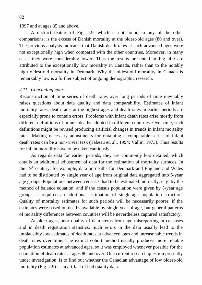
82
1997 and at ages 35 and above.A distinct feature of Fig. 4.9, which is not found in any of the other
comparisons, is the excess of Danish mortality at the oldest-old ages (80 and over).The previous analysis indicates that Danish death rates at such advanced ages werenot exceptionally high when compared with the other countries. Moreover, in manycases they were considerably lower. Thus the results presented in Fig. 4.9 areattributed to the exceptionally low mortality in Canada, rather than to the notablyhigh oldest-old mortality in Denmark. Why the oldest-old mortality in Canada isremarkably low is a further subject of ongoing demographic research.
4.11 Concluding notes
Reconstruction of time series of death rates over long periods of time inevitablyraises questions about data quality and data comparability. Estimates of infantmortality rates, death rates at the highest ages and death rates in earlier periods areespecially prone to contain errors. Problems with infant death rates arise mostly fromdifferent definitions of infants deaths adopted in different countries. Over time, suchdefinitions might be revised producing artificial changes in trends in infant mortalityrates. Making necessary adjustments for obtaining a comparable series of infantdeath rates can be a non-trivial task (Tabeau et. al., 1994; Vallin, 1973). Thus resultsfor infant mortality have to be taken cautiously.
As regards data for earlier periods, they are commonly less detailed, whichentails an additional adjustment of data for the estimation of mortality surfaces. Inthe 19th century, for example, data on deaths for Denmark and England and Waleshad to be distributed by single year of age from original data aggregated into 5-yearage groups. Populations between censuses had to be estimated indirectly, e. g. by themethod of balance equation, and if the census population were given by 5-year agegroups, it required an additional estimation of single-age population structure.Quality of mortality estimates for such periods will be necessarily poorer, if theestimates were based on deaths available by single year of age, but general patternsof mortality differences between countries will be nevertheless captured satisfactory.
At older ages, poor quality of data stems from age misreporting in censusesand in death registration statistics. Such errors in the data usually lead to theimplausibly low estimates of death rates at advanced ages and unreasonable trends indeath rates over time. The extinct cohort method usually produces more reliablepopulation estimates at advanced ages, so it was employed whenever possible for theestimation of death rates at ages 80 and over. One current research question presentlyunder investigation, is to find out whether the Canadian advantage of low oldest-oldmortality (Fig. 4.9) is an artifact of bad quality data.

83
Certain problems also arise from different classification schemes adopted by theNational Statistical Offices. For example, deaths could be classified either by singleyear and age, as in England and Wales, or by single year of birth and age, as in thecase of Norway. Distributing deaths by Lexis triangles introduces an additional biasin mortality estimates.
Despite all the problems with the reconstruction of mortality trends overextended periods of time, the results presented in this chapter can be consideredreliable. Before the analysis, all raw data were scrutinized and subjected to variousquality checks. Only data, which appeared to be reasonable, were included in thepresent analysis. In addition, all of the countries selected for the analysis have a longtradition of collecting population and vital statistics and are consequently consideredreliable by the demographic community. Altogether, it allows us to make thefollowing conclusions.
First, I would like to note that the analysis presented in this chapter, helped usto look at the mortality developments in Denmark for more than 150 years and froman international perspective. An examination revealed some remarkable features inthe Danish mortality evaluation. In the second half of 19th century, the mortalitytransition in Denmark was among the mainstream of European countries. Danishdeath rates were somewhat higher than those in Sweden and Norway, but lower thanthe death rates in the Netherlands and England and Wales. One exception from thispattern, is the age group 5–15, where the death rates in Denmark for both sexes weresignificantly higher than in other countries. By the end of the 19th century, the Danishmortality disadvantage in this age group, however, appears to sharply diminish anddisappear.
In the first half of the 20th century, mortality conditions in Denmark were quitefavorable. The rapid mortality decline secured a place for Denmark among thelongest-lived countries. Danish mortality advantage at childhood, young and youngadult ages (<60) were so obvious during the first decades of the 20th century, thatDanish life expectancy at birth was perhaps the highest among European countries.This is consistent with findings presented by Vallin (Table 3.2). There is someevidence, however, that the Danish female death rates at adult ages were slightlyhigher than those in other countries. Nevertheless this disadvantage cannotsignificantly influence the estimates of the life expectancy at birth, because the deathrates at younger ages were still rather high and their influence on estimates of lifeexpectancy at birth was the highest among all ages.
In the second half of the 20th century, the Danish mortality advantage to alarge extent disappeared, which resulted in the emergence of areas with abundant

84
Danish mortality at the middle ages. Particular unfavorable developments werefound in the population of females, where death rates started to lag behind those inother developed countries by the 1970s. For males, a similar phenomenon is to beobserved as well, but it is less outstanding and it came only into view during the1980s. Due to the unfavorable trends in Danish mortality, female death ratesappeared to be the highest among all countries in the last several years at ages 40–80and male death rates at ages 60–80.
Figures 4.10 and 4.11 make it easier to comprehend the results summarized inthis section. Fig. 4.10 shows years and ages where death rates in Denmark were thehighest among all countries for which data were available in the given period. Fig.4.11, shows years and ages where the death rates were the lowest. Excess of femalemortality in the period 1970–1999 (Fig. 4.10) and Danish mortality advantage in theperiod 1900–1950 (Fig. 4.11) appear especially eye-catching.
The Danish mortality disadvantage in the recent years is a notablephenomenon and it definitely calls for explanation. One way to gain a deeperunderstanding about the factors behind the excess of Danish mortality is to examinethe trends in cause-specific mortality. For obvious reasons, data on the causes ofdeath are less reliable and less detailed than those analyzed here, but we are nowconcerned with statistics for recent decades, where data quality should be reasonablygood to draw some useful conclusions. This is subject of the following chapter.

1860 1880 1900 1920 1940 1960 198019990
102030405060708090
100Males
Year
Age
The highest death rates in Denmark compared with other countriesFigure 4.10.
85
1860 1880 1900 1920 1940 1960 198019990102030405060708090100
Females
Year
1860 1880 1900 1920 1940 1960 198019990
102030405060708090
100Males
Year
Age
The lowest death rates in Denmark compared with other countriesFigure 4.11.
1860 1880 1900 1920 1940 1960 198019990102030405060708090100
Females
Year

86

87
5. Cause-specific mortality
5.1 An analysis of cause-specific mortality
One of the main findings, described in the previous chapter, is the unusual excess ofDanish mortality in recent years. This phenomenon can be investigated in differentways. An analysis of the causes of death is one of the most important directions forfurther research. For my comparison, I have selected three countries: Sweden, theNetherlands and Japan. Sweden is chosen to represent the experience of the Nordiccountries and the Netherlands is to represent the central part of Europe. Japan isinteresting, since differences between Danish and Japanese death rates are now thehighest, when compared to the other countries.
The mortality database maintained by the World Health Organization (WHO)includes death counts classified by causes of death for all countries throughout theworld. Utilizing such data makes it possible for us to analyze cause-specificmortality differences between countries. These data have been used extensively instudies devoted to the stagnation of Danish life expectancy (SundhedsministerietsMiddellevetidsudvalg, 1993; Bjerregaard and Juel, 1993; Bjerregaard and Juel,1994). The analysis presented in this section has two main objectives. The first goalis to decompose excess Danish mortality by causes of deaths, in order to reveal thecauses of death contributing most to the excess of Danish mortality. The second is tosurvey the trends in cause-specific death rates.
For this purpose, I have downloaded the mortality data from the WHO website17 and extracted the relevant country-specific data from the raw mortality files.Then, I created an abridged list of 25 causes of deaths (Appendix Table 8) andaggregated the death counts using this custom classification. The causes of deathsincluded in the abridged list, were selected after a careful examination of scientificpublications related to the current analysis.
The method of excess mortality decomposition that I used here is very simple,and the interpretation of the results is based on the assumption of the independenceof causes of death. The relative excess mortality for a given period and in a certainage group can be computed as
ρ =′
−
⋅m
m1 100% (5.1)
where m and ′m are the central death rates (cf. e.g. Chiang, 1984) in Denmark andthe country selected for comparison, respectively. The ratio of death rates is then:
17 www.who.int/whosis/mort/

88
m
m
m
m m
ii
ii
ii
ii
′=
′= +
′
∑∑
∑∑1
∆ (5.2)
where mi is the mortality rate from the ith cause of death and ∆ i i im m= − ′ is the
absolute difference in mortality from the ith cause of death in Denmark and another
country. Finally,ρ ρ= ∑ i
i
(5.3)
where ρii
ii
m=
′⋅
∑∆
100% is the contribution of the ith cause of death in the total excess
mortality.As can be seen in Fig. 4.10, the most striking differences in mortality are
observed at ages 50–70, and this pattern has remained more or less stable since 1970.Following this observation, I applied this method to decompose the mortalitydifferences in Denmark and other countries for the period 1985–1993, for 4 agegroups: 50–54, 55–59, 60–64 and 65–69. Table 5.1 shows the computed values of ρi
by cause of death, age group, sex, and country. The last row of the table shows thetotal excess mortality (equation 5.1). For example, female death rates in Denmark inthe period 1985–1993 for ages 60–64 were on average 58.62% higher than inSweden (Table 5.1). The 9.65% out of 58.62% are attributed to lung cancer (cause 2;Malignant neoplasm of trachea, bronchus and lungs; Appendix Table 8); 5.28% tobreast cancer (cause 7) etc. Positive values of ρi , which indicate a significant
contribution to excess mortality (>2%), have been highlighted to facilitate thereading of this table. I must also note that two sets of estimates of excess mortality,(based on WHO data and on the data published by the national statistical offices) arein agreement for all populations, but the Netherlands. For the male and femalepopulations of the Netherlands, excess Danish mortality is somewhat higher if it isestimated from the WHO data.
Table 5.1 contains a great deal of material, which the interested reader willwish to examine for him or herself. Here a few general comments:
a) Denmark vs. Sweden, Males. The main contribution to excess Danish
mortality stems from the higher mortality from lung cancer (cause 2).Approximately 25% of the overall excess mortality can be attributed to thiscase of death. Higher mortality from the residual group of neoplasm (8) is alsoapparent in all age groups, but its contribution is less substantial and itdecreases with age. In the lower age groups (50–64), mortality from ischaemic

89
heart disease (9), cirrhosis of the liver (18) and suicide (21) is alsosignificantly higher in Denmark. At ages 65–69, contribution of these causesof deaths to the total mortality excess is, however, quite small. On the contrary,excess mortality from respiratory diseases (15) increases sharply with age. Atages 60–69, it accounts for about 15% of the total excess.
b) Denmark vs the Netherlands, Males. The two most important causes of death
with higher Danish mortality are the residual neoplasm group (8) andischaemic heart disease (9). The latter accounts for about 20% of the totalexcess mortality at ages 50–54 and 45% at ages 64–69; the residual neoplasmgroup makes up approximately 15% of the excess mortality. In contrast tocomparisons with other populations, mortality from lung cancer is actuallylower in Denmark than in the Netherlands. This finding is rather surprising,since a higher mortality from lung cancer in Denmark has been observed in allother comparisons - for both the male and female populations. In the age group50–54, where excess Danish mortality was the highest, significant differencesare to be seen in death rates from cirrhosis of the liver (18) and as well suicide(21). The contribution of these causes of death to excess mortality declineswith age and becomes negligible in higher age groups.
c) Denmark vs Japan, Males. In this comparison, the analysis reveals striking
differences in the mortality from ischaemic heart disease (9), which isresponsible for about 70% of the excess Danish mortality. The next importantcause of death is lung cancer (2), which is also appreciably higher in Denmarkthan in Japan. The third important cause contributing to excess mortality isdisease of the respiratory system (15).
d) Denmark vs Sweden, Females. The highest mortality differences exist in the
area of cancer, especially lung cancer (2), residual cancers (8) and breastcancer (7). Altogether, these 3 causes of death account for about 40% of theobserved excess mortality. Other important contributors to excess Danishmortality are respiratory diseases (15) and ischaemic heart disease (9). Thecontribution to excess mortality from the group ‘Bronchitis, emphysema andasthma’ (15) is noticeably higher than from ischaemic heart disease (9), and itis as important as lung cancer, at ages 65–69. At ages 50–59, we can also seethe marked differences in death rates from cirrhosis of the liver (18) andsuicide (21). At higher ages, mortality differences from these causes of deathare less pronounced. An excess of mortality from cerebrovascular disease (11)is also noticeable, although its contribution seems to be less significant thanfrom the causes mentioned above.

90
Table 5.1 Decomposition of excess Danish mortality by causes of death for the
period 1985–1993. Males.
The table shows the contribution of a particular cause of death to the total excessmortality (%). A description of the causes of death together with the WHO categorynumbers is provided in Appendix Table 8. Causes of death contributing more than2% to excess mortality appear in boldface type.
Cause Sweden Netherlands JapanAges 50–54 55–59 60–64 65–69 50–54 55–59 60–64 65–69 50–54 55–59 60–64 65–69
1 1.12 0.47 0.11 -0.12 1.25 0.69 0.11 -0.05 -0.08 -0.70 -1.15 -1.502 5.86 8.49 9.48 8.87 -1.46 -0.89 -1.10 -1.71 7.11 9.96 10.11 9.273 0.02 0.13 -0.23 -0.34 0.40 0.78 0.71 1.25 0.79 1.662.52 3.944 0.27 0.78 1.04 1.11 -0.23 0.45 0.57 0.31 0.06 0.65 1.14 1.40
5 0.50 0.15 0.01 -0.30 -0.25 -0.65 -0.82 -0.79 -6.63 -7.50 -7.98 -7.80
6 0.52 0.87 0.82 1.11 0.64 1.18 1.12 1.31 -0.27 0.20 0.38 1.12
7 0.09 0.08 0.07 0.05 0.09 0.09 0.07 0.05 0.09 0.09 0.08 0.06
8 6.71 5.18 5.03 3.82 5.53 4.52 4.22 3.05 2.57 -0.87 0.47 2.32
9 4.70 4.17 2.16 0.62 8.18 10.56 10.34 10.76 26.12 32.27 36.63 38.9510 -0.70 -0.55 0.01 -0.28 -2.43 -2.32 -2.13 -2.72 -6.10 -5.15 -4.48 -4.98
11 1.31 0.58 0.95 0.88 1.95 1.66 1.80 1.52 -6.11 -4.91 -3.37 -2.67
12 0.58 0.17 0.77 0.42 0.76 0.13 0.33 -0.04 1.35 1.492.77 3.3513 0.86 1.15 1.21 1.14 0.98 1.25 1.45 1.37 1.03 1.47 1.922.04
14 -1.36 -1.05 -0.74 -0.70 0.22 0.38 0.38 0.35 -1.25 -1.58 -2.52 -3.9215 1.40 3.02 4.47 5.30 1.42 2.41 2.51 2.18 2.00 3.99 6.04 7.4916 0.01 0.01 0.06 0.01 -0.02 0.01 0.03 0.00 0.02 0.03 0.08 0.06
17 0.39 0.10 0.18 0.26 0.37 0.19 0.29 0.19 -0.29 -0.64 -0.80 -1.12
18 4.67 2.89 1.63 1.03 5.96 4.25 2.39 1.26 -0.12 -0.59 -0.44 -0.2619 -0.10 -0.03 0.19 0.18 0.42 0.39 0.44 0.45 0.13 0.15 0.38 0.47
20 -0.58 -0.05 0.06 0.09 -0.01 0.12 -0.11 -0.19 -0.84 -0.52 -0.48 -0.29
21 3.16 1.54 1.42 0.70 7.10 3.50 2.26 1.23 1.87 0.88 1.32 0.7522 1.10 0.35 0.44 0.28 1.09 0.49 0.51 0.25 -0.16 -0.54 -0.19 -0.27
23 -0.17 -0.25 -0.02 0.11 0.55 0.31 0.40 0.32 -0.14 -0.19 0.12 0.26
24 -2.91 -1.87 -1.49 -0.71 2.68 1.48 0.62 0.31 -0.35 -0.64 -0.97 -0.96
25 9.88 9.34 7.97 6.44 8.95 6.85 4.80 2.96 14.56 12.67 10.61 8.86
Total 37.35 35.66 35.60 29.98 44.15 37.85 31.19 23.63 35.34 41.69 52.19 56.59

91
Table 5.1 (cont.) Females.
Cause Sweden Netherlands JapanAges 50–54 55–59 60–64 65–69 50–54 55–59 60–64 65–69 50–54 55–59 60–64 65–69
1 0.26 0.28 0.04 -0.10 0.30 0.43 0.22 0.13 -0.47 -0.49 -0.85 -0.772 8.58 12.58 9.65 7.15 9.21 12.63 10.24 9.15 14.04 19.31 15.27 10.803 0.00 0.00 0.00 0.00 0.00 0.00 0.00 0.00 0.00 0.00 0.00 0.00
4 1.65 2.19 1.84 1.34 1.19 1.89 1.37 0.78 2.32 3.51 3.23 2.835 -0.20 0.42 -0.23 -0.54 0.12 0.73 -0.04 -0.35 -7.28 -5.82 -5.94 -5.49
6 0.78 0.92 1.11 0.84 1.20 1.46 1.74 1.52 0.34 0.93 1.48 1.28
7 9.14 7.77 5.28 3.72 4.41 4.37 2.35 1.72 19.81 18.98 14.47 10.478 8.52 9.23 8.63 4.50 13.31 14.28 13.74 9.80 20.19 23.97 22.22 16.50
9 4.08 5.60 5.45 3.57 4.13 6.54 9.57 10.50 11.92 18.71 25.07 27.3210 -0.37 -0.59 0.17 -0.17 -1.57 -1.89 -1.45 -2.48 -4.97 -5.00 -4.72 -6.19
11 2.84 2.45 1.94 1.69 3.00 2.64 3.17 2.75 -3.47 -2.96 -2.15 -2.43
12 1.15 0.78 0.96 1.06 1.39 1.20 1.47 1.90 1.81 1.962.50 3.1613 1.44 1.68 1.66 1.44 1.65 1.61 1.73 1.95 1.872.25 2.44 2.56
14 -0.08 -0.19 -0.41 -0.39 0.58 0.60 0.55 0.69 -0.48 -0.95 -1.41 -2.2415 4.70 7.04 7.78 6.85 5.06 7.63 8.60 7.62 7.05 11.04 12.74 11.0016 0.04 0.12 0.07 0.08 0.03 0.07 0.02 0.06 0.05 0.17 0.12 0.13
17 0.15 0.30 0.20 0.05 0.15 0.45 0.39 0.26 -0.38 -0.16 -0.34 -0.59
18 3.61 2.23 1.54 0.69 4.34 2.97 2.12 0.98 4.02 1.85 0.54 -0.7019 0.61 0.66 0.73 0.67 0.95 0.86 1.01 1.05 1.00 1.05 1.22 1.17
20 0.12 0.47 0.44 0.39 0.27 0.44 0.27 0.13 0.40 0.57 0.68 0.40
21 6.14 3.97 2.63 1.55 8.33 5.09 3.05 1.98 6.98 4.51 2.51 1.0122 0.56 0.12 0.19 0.31 0.88 0.40 0.27 0.22 0.25 -0.16 -0.18 -0.13
23 0.20 0.34 0.48 0.43 0.24 0.27 0.52 0.70 0.38 0.53 0.85 1.03
24 1.27 0.00 -0.31 -0.07 4.27 1.95 1.07 0.58 3.74 1.34 0.32 -0.28
25 9.67 10.68 8.76 8.45 8.91 7.79 5.41 4.29 15.36 15.87 13.29 11.91
Total 64.86 69.05 58.62 43.52 72.37 74.39 67.41 55.95 94.48 111.02 103.35 82.75
e) Denmark vs the Netherlands, Females. The general structure of the cause-
specific excess mortality is quite similar to that found when comparing Danishand Swedish data. However, mortality differences in ischaemic heart disease(9) at high ages and the differences in suicide (21) mortality in the lower agegroups are higher than those found in the comparison to Sweden.
f) Denmark vs Japan, Females. Similar to the comparisons with Sweden and
Denmark, the analysis indicates that the following causes of deaths are themost significant contributors to excess of Danish mortality: lung cancer (2),breast cancer (7), residual malignant neoplasm (8), ischaemic heart disease (9),

92
and respiratory diseases (15). In addition, at ages 50–59, a substantialcontribution is also provided by the differences in mortality from cirrhosis ofthe liver (18) and suicide (21).
The residual group of diseases (25) includes the remaining causes of death, whichhave not been classified in any of the other 24 categories (Appendix Table 8). As canbe seen in Table 5.1, these residual causes of death also provide an appreciablecontribution to excess Danish mortality for all countries and for all age groups. Therelative importance of the causes of death in a group (25) reflects, above all, the factthat different diagnostic and coding practices have been adopted in the differentcountries. In the case of Denmark, there is a relatively high proportion of deaths thatare classified as unknown or ill-defined cases.
If precise diagnostics were possible, one might expect that the absolutecontributions to excess Danish mortality from the specific causes of deaths would beeven higher, since more deaths would be allocated to the specific disease categories.However, the relative contribution of a particular cause of death to excess Danishmortality in this case, might thereby change.
In sum, the results presented in Table 5.1 should be considered suggestive, butnot conclusive. The problem we are facing here is rooted in the quality of data oncause-specific mortality. In addition to the large group of residual diseases, theresults related to the diseases of the circulatory and the respiratory systems(Appendix Table 7, chapters III and IV) should be viewed with greater caution thanothers (Juel and Sjol, 1995; Bjerregaard and Juel, 1993).
Yet another source of errors is the different classifications of diseases used bycountries submitting data to the WHO. This sometimes makes it difficult to restoretime trends of specific causes of deaths. Denmark used the 8th revision of theInternational Classification of Disease (ICD) from 1969 to 1993, while in theNetherlands and Japan, this classification was used only up until 1979 and inSweden until 1987. After these dates, death counts were reported in these countriesusing the 9th revision of the ICD. In contrast, Denmark never made of use the 9th
revision of the ICD, but has used the 10th revision since 1994. Here is one example ofthe problems associated with the transition from the 8th to the 9th revision: in Japan,this resulted in an abrupt jump in death rates from the 10th cause of death (otherforms of heart disease); a similar jump is also noticeable in the Netherlands, but notin Sweden.
To minimize the effect of problems associated with misclassification and toimprove the overall quality of results, I aggregated the causes of deaths by disease

93
categories included in the chapters of Appendix Table 8. By aggregating the data, it
is possible to obtain more reliable results, but the structure of those causes of deaththat provide contributions to excess Danish mortality will be less detailed. I repeatedthe procedure described above, using these broader categories of diseases. Inaddition, I computed the relative contribution of a particular cause of death to excess
Danish mortality and included it in Table 5.2. The highlighted items in Table 5.2 arethe causes of death that provide the highest contribution to the excess Danishmortality.
As is evident from Table 5.2, there are striking similarities among the resultsfor the female populations. In all countries and at all ages, excess mortality fromcancer (group II) has made the highest contribution to the observed mortalitydifferences. The numbers range from 40 to 50% of total excess mortality.Cardiovascular diseases (III) and respiratory diseases (IV) take second and thirdplace, respectively, in order of importance. At ages 50–54, however, the mostimportant contribution (after cancer) comes from mortality from accidents,poisonings, and violence (VI), leaving the cardiovascular and respiratory diseasesbehind.
The results obtained for male populations are less homogeneous between thecountries. However, in the case of Sweden, the pattern is similar to that observed inthe female populations, i.e., the main contribution is attributed to cancer mortalityfollowed by cardiovascular mortality and mortality from respiratory diseases.Generally, about 45% of excess mortality is related to cancer. We also note that theimportance of respiratory diseases rises significantly with age and that this is the agegroup 65–69, where mortality differences are more pronounced. In addition, at ages50–54 the group of digestive diseases, including cirrhosis of the liver, constitutes asignificant part of excess mortality.
As follows from Table 5.2, the male population of Japan has a strikingadvantage of lower mortality from cardiovascular diseases. The differences in deathrates from cancer, also provide a positive contribution to excess Danish mortality,but this is less marked. Approximately 60% of the excess mortality (Denmark vs.Japan) can be attributed to cardiovascular diseases, 15% to malignant neoplasms andabout 4% to respiratory diseases. The Japanese levels of mortality from other causesof death are comparable with the Danish levels.
Compared to the male population of the Netherlands, the most notablemortality differences are to be observed in cardiovascular mortality (III). Death ratesfrom this cause of death account for 30% of the total mortality differences at ages55–59 and about 45% at ages 65–69. However, at ages 50–54, the highest

94
contribution did not come from the cardiovascular diseases, but from accidents (VI),which accounted for 25% of the total excess mortality. With advancing age, theimportance of accidents falls, while contribution of cancers (II) and diseases ofrespiratory system (IV) increases. Altogether, these causes of death account for 26%of the total mortality excess at ages 65–69.
5.2 Time trends in cause-specific mortality
The analysis presented in the previous section helped us to highlight the mostimportant causes of death contributing to excess Danish mortality in middle age.Another question of principal interest involves trends in death rates from specificcauses of death. I have computed the series of death rates for the period from 1970 to1993 by 4 age groups for all countries included in the analysis. The year 1970 was
Table 5.2 Decomposition of excess Danish mortality by aggregated causes of death
for the period 1985–1993. Males.
The table shows both the absolute and relative contribution (%) of a particular groupof diseases to the total excess mortality. A description of causes of death included ina particular group of diseases is provided in Appendix Table 8. The items in boldfaceare causes of death providing maximal contributions to excess mortality.Chapter Sweden Netherlands JapanAges 50–54 55–59 60–64 65–69 50–54 55–59 60–64 65–69 50–54 55–59 60–64 65–69
Absolute contribution to excess mortality(%)I 1.12 0.47 0.11 -0.12 1.25 0.69 0.11 -0.05 -0.08 -0.70 -1.15 -1.50II 13.97 15.68 16.22 14.31 4.73 5.48 4.77 3.47 3.70 4.19 6.72 10.32
III 6.75 5.52 5.11 2.78 9.4411.29 11.79 10.88 16.28 25.17 33.47 36.69IV 0.44 2.08 3.97 4.88 2.00 2.99 3.21 2.72 0.48 1.80 2.79 2.51
V 4.00 2.81 1.88 1.31 6.37 4.77 2.72 1.53 -0.82 -0.96 -0.54 -0.07
VI 1.19 -0.24 0.34 0.3711.42 5.78 3.80 2.11 1.22 -0.48 0.29 -0.22
VII 9.88 9.34 7.97 6.44 8.95 6.85 4.80 2.96 14.56 12.67 10.61 8.86
Total 37.35 35.66 35.60 29.98 44.15 37.85 31.19 23.63 35.34 41.69 52.19 56.59
Relative contribution to excess mortality (%)
I 2.99 1.33 0.31 -0.40 2.83 1.83 0.34 -0.20 -0.23 -1.68 -2.21 -2.65II 37.40 43.98 45.55 47.75 10.71 14.48 15.28 14.70 10.48 10.04 12.88 18.23
III 18.08 15.47 14.34 9.28 21.3829.82 37.79 46.06 46.07 60.37 64.14 64.84IV 1.17 5.83 11.14 16.27 4.53 7.91 10.30 11.53 1.35 4.33 5.35 4.44
V 10.71 7.87 5.29 4.36 14.43 12.59 8.71 6.46 -2.33 -2.30 -1.04 -0.13
VI 3.18 -0.67 0.97 1.2525.86 15.27 12.18 8.93 3.46 -1.15 0.56 -0.38
VII 26.46 26.19 22.40 21.49 20.26 18.09 15.40 12.52 41.19 30.38 20.33 15.66
Total 100.00 100.00 100.00 100.00 100.00 100.00 100.00 100.00 100.00 100.00 100.00 100.00

95
Table 5.2 (cont.) Females.
Chapter Sweden Netherlands JapanAges 50–54 55–59 60–64 65–69 50–54 55–59 60–64 65–69 50–54 55–59 60–64 65–69
Absolute contribution to excess mortality(%)I 0.26 0.28 0.04 -0.10 0.30 0.43 0.22 0.13 -0.47 -0.49 -0.85 -0.77II 28.47 33.11 26.28 17.00 29.44 35.35 29.41 22.63 49.42 60.88 50.73 36.38III 9.14 9.92 10.19 7.59 8.60 10.10 14.50 14.61 7.16 14.96 23.13 24.42
IV 4.80 7.26 7.64 6.59 5.83 8.74 9.57 8.64 6.24 10.10 11.11 8.30
V 4.35 3.36 2.71 1.76 5.57 4.27 3.40 2.17 5.41 3.48 2.45 0.87
VI 8.17 4.43 2.99 2.22 13.72 7.71 4.92 3.49 11.35 6.22 3.50 1.63
VII 9.67 10.68 8.76 8.45 8.91 7.79 5.41 4.29 15.36 15.87 13.29 11.91
Total 64.86 69.05 58.62 43.52 72.37 74.39 67.41 55.95 94.48111.0 103.35 82.75
Relative contribution to excess mortality (%)
I 0.40 0.41 0.07 -0.23 0.41 0.58 0.32 0.24 -0.50 -0.44 -0.82 -0.94II 43.90 47.95 44.84 39.06 40.68 47.53 43.62 40.44 52.31 54.84 49.08 43.97III 14.10 14.36 17.39 17.44 11.88 13.57 21.50 26.12 7.58 13.47 22.38 29.51
IV 7.40 10.52 13.03 15.15 8.06 11.75 14.19 15.44 6.61 9.10 10.75 10.03
V 6.70 4.87 4.63 4.05 7.70 5.74 5.05 3.87 5.73 3.13 2.37 1.05
VI 12.60 6.42 5.10 5.11 18.96 10.37 7.29 6.23 12.01 5.60 3.39 1.97
VII 14.90 15.47 14.94 19.42 12.31 10.47 8.02 7.66 16.26 14.30 12.86 14.40
Total 100.0 100.0 100.0 100.0 100.0 100.0 100.0 100.00 100.0 100.0 100.00 100.0
chosen, because it marks the emergence of the area of excess mortality, as can beseen in Fig. 4.10. In addition, all countries used the 8th revision of the ICD at thattime, which permits us to avoid certain classification problems in the earlier years.Altogether, 200 plots18 have been analyzed and 44 of them displaying thedisadvantageous trends in Danish mortality are presented in Fig. 5.1(a,b). It must be
emphasized, that the causes of deaths discussed below have been selected in order toshed light on Danish excess mortality. In other words, only causes of death, whereDanish mortality is higher, are discussed here. The reader interested in the trends ofall causes of death can explore the graphs provided on the CD-ROM for him orherself.
Male mortality from lung cancer (2) has been steadily increasing in Denmark,Sweden and Japan (except ages 50–54), but not in the Netherlands, here a moderatedecline in mortality can be observed (Fig. 5.1(a)). During the whole period, Danishmortality has been double that of Sweden and Japan, but appreciably lower than thatof the Netherlands. The decline in Dutch mortality led to the convergence of
18 The plots with the trends in cause-specific mortality are provided on the accompanying CD-ROM. The files are stored in HTML format and can
be viewed with any Web browser. If your CD-ROM drive is assigned the D: letter, open D:\CAUSES\CAUSE.HTM to start browsing.

96
Malignant neoplasm of the trachea, bronchus and lungs(2). Males
Death rates at ages 50-54
0
50
100
150
1970 1975 1980 1985 1990 1995Year
Mor
talit
y *
100,
000
DkSwNlJp
Death rates at ages 55-59
0
50
100
150
200
250
1970 1975 1980 1985 1990 1995Year
Mor
talit
y *
100,
000
Death rates at ages 60-64
0
100
200
300
400
1970 1975 1980 1985 1990 1995Year
Mor
talit
y *
100,
000
Death rates at ages 65-69
0
100
200
300
400
500
600
1970 1975 1980 1985 1990 1995Year
Mor
talit
y *
100,
000
Ischaemic heart disease(9). Males
Death rates at ages 50-54
0
100
200
300
1970 1975 1980 1985 1990 1995Year
Mor
talit
y *
100,
000
DkSwNlJp
Death rates at ages 55-59
0
100
200
300
400
500
600
1970 1975 1980 1985 1990 1995Year
Mor
talit
y *
100,
000
Death rates at ages 60-64
0
200
400
600
800
1000
1970 1975 1980 1985 1990 1995Year
Mor
talit
y *
100,
000
Death rates at ages 65-69
0
200
400
600
800
1000
1200
1400
1970 1975 1980 1985 1990 1995Year
Mor
talit
y *
100,
000
Figure 5.1(a) Disadvantageous trends in Danish cause-specific mortality. Males.

97
Bronchitis, emphysema and asthma(15). Males
Death rates at ages 50-54
0
10
20
30
40
50
1970 1975 1980 1985 1990 1995Year
Mor
talit
y *
100,
000
DkSwNlJp
Death rates at ages 55-59
0
20
40
60
80
100
1970 1975 1980 1985 1990 1995Year
Mor
talit
y *
100,
000
Death rates at ages 60-64
0
50
100
150
1970 1975 1980 1985 1990 1995Year
Mor
talit
y *
100,
000
Death rates at ages 65-69
0
50
100
150
200
250
1970 1975 1980 1985 1990 1995Year
Mor
talit
y *
100,
000
Cirrhosis of liver(18). Males
Death rates at ages 50-54
0
20
40
60
80
100
1970 1975 1980 1985 1990 1995Year
Mor
talit
y *
100,
000
DkSwNlJp
Death rates at ages 55-59
0
20
40
60
80
100
1970 1975 1980 1985 1990 1995Year
Mor
talit
y *
100,
000
Death rates at ages 60-64
0
20
40
60
80
100
1970 1975 1980 1985 1990 1995Year
Mor
talit
y *
100,
000
Death rates at ages 65-69
0
20
40
60
80
100
1970 1975 1980 1985 1990 1995Year
Mor
talit
y *
100,
000
Figure 5.1(a) (cont.)

98
Suicide and self inflicted injury(21). Males
Death rates at ages 50-54
0
20
40
60
80
100
1970 1975 1980 1985 1990 1995Year
Mor
talit
y *
100,
000
Death rates at ages 55-59
0
20
40
60
80
100
1970 1975 1980 1985 1990 1995Year
Mor
talit
y *
100,
000
DkSwNlJp
Death rates at ages 60-64
0
20
40
60
80
100
1970 1975 1980 1985 1990 1995Year
Mor
talit
y *
100,
000
Death rates at ages 65-69
0
20
40
60
80
100
1970 1975 1980 1985 1990 1995Year
Mor
talit
y *
100,
000
Figure 5.1(a) (cont.)
mortality levels in the Danish and Dutch populations, so there is much lessdifference between the two countries at the beginning of 1990s than in the 1970s.Moreover, there is a certain drop in the death rates at ages 50–54 for both Denmarkand the Netherlands; this can perhaps be attributed to certain cohort effects, but thishypothesis requires additional elaboration.
Trends in death rates from ischaemic heart disease (9) followed almost thesame trajectory in all European countries. Until 1980, the death rates remained at anapproximately constant level, but after 1980, a persistent decline can be observed inall populations. The rate of decline was appreciable, and by the year 1993, the levelof mortality had dropped to nearly half that of 1980. The level of mortality nowdiffers considerably between countries and age groups. Even though it followed thesame pattern of decline, in the lower age groups (50–54), Danish mortality wasgenerally higher than that of Sweden and the Netherlands. In contrast, at higher ages(60–69), Danish and Swedish mortality curves are very close, while Dutch mortalityis significantly lower. The exceptionally low level of Japanese mortality makes theposition of this country outstanding in comparison. Mortality in Japan has alsodeclined, but its level was significantly lower (4- to 6-fold) than in Europeancountries.

99
Regarding respiratory diseases, we observe that there are no notable trends in Danishmortality from this cause of death. This is true of Sweden as well, although mortalityin Denmark was on average 2.5 times higher than in Sweden. A comparison betweenDenmark and the Netherlands shows that in the early 1970s, mortality in bothcountries was nearly the same but in the early 1990s Danish death rates were about50% higher because of the reductions in Dutch mortality. The death rates in Japanalso show a downward trend, but their level was comparable with the Swedish levelin the 1970s, which is appreciably lower than in the Netherlands. Because of thisdecline, the level of Japanese mortality in recent years has been the lowest of allcountries included in the comparison.
In the case of cirrhosis of the liver (18), the trend in Danish mortality is theopposite of that observed in the other countries. I found a substantial and uniformincrease in all age groups in Denmark, while mortality in Sweden dropped sharply inthe early 1980s and mortality in Japan remained either constant (50–59) or declining(60–69). Even though Japanese mortality was remarkably higher than in the Nordiccountries in 1970, the level of mortality in Denmark and in Japan was virtually thesame in the 1993. Mortality in Sweden at that time was about half of that. In theNetherlands, no notable trends in mortality can be observed; it remained constant atlow level.
Death rates from suicide (21) have traditionally been higher in Danish malesthan in other countries. There have been no considerable improvements here, exceptfor some convergence to the levels of Sweden and the Netherlands at ages 55–64 inrecent years. It is difficult to judge whether this is the onset of a general trend orsome temporary phenomenon, because there is no evidence of a similar decline atages 50–54 or 65–69.
In the populations of females, causes of deaths exhibiting unfavorabledevelopments in Denmark, turn out to be the same as for males. Therefore, we willdiscuss the same causes of death as for males, adding only the trends in breastcancer. In the case of lung cancer mortality (2), there is a remarkable gap betweenthe Danish population and other countries. Mortality from lung cancer has beenincreasing in all countries since 1970 and the rate of increase has been especiallylarge in Europe (8.5% in Denmark and the Netherlands; 6.5% in Sweden) as opposedto Japan (1%). Mortality in Denmark, in the early 1970s, was appreciably higherthan in other countries and this difference has increased in the 1990s, even thoughthe Danish rate of increase was approximately the same as that of Sweden and theNetherlands.
Breast cancer death rates (7) have been gradually increasing in Denmark and

100
Malignant neoplasm of the trachea, bronchus and lungs(2). Females
Death rates at ages 50-54
0
20
40
60
1970 1975 1980 1985 1990 1995Year
Mor
talit
y *
100,
000
Death rates at ages 55-59
0
50
100
150
1970 1975 1980 1985 1990 1995Year
Mor
talit
y *
100,
000
DkSwNlJp
Death rates at ages 60-64
0
50
100
150
200
1970 1975 1980 1985 1990 1995Year
Mor
talit
y *
100,
000
Death rates at ages 65-69
0
50
100
150
200
1970 1975 1980 1985 1990 1995Year
Mor
talit
y *
100,
000
Malignant neoplasm of breast(7). Females
Death rates at ages 50-54
0
20
40
60
80
100
1970 1975 1980 1985 1990 1995Year
Mor
talit
y *
100,
000
Death rates at ages 55-59
0
50
100
150
1970 1975 1980 1985 1990 1995Year
Mor
talit
y *
100,
000
DkSwNlJp
Death rates at ages 60-64
0
50
100
150
1970 1975 1980 1985 1990 1995Year
Mor
talit
y *
100,
000
Death rates at ages 65-69
0
50
100
150
1970 1975 1980 1985 1990 1995Year
Mor
talit
y *
100,
000
Figure 5.1(b) Disadvantageous trends in Danish cause-specific mortality. Females.

101
Ischaemic heart disease(9). Females
Death rates at ages 50-54
0
20
40
60
1970 1975 1980 1985 1990 1995Year
Mor
talit
y *
100,
000
Death rates at ages 55-59
0
50
100
150
1970 1975 1980 1985 1990 1995Year
Mor
talit
y *
100,
000
Death rates at ages 60-64
0
100
200
300
1970 1975 1980 1985 1990 1995Year
Mor
talit
y *
100,
000
Death rates at ages 65-69
0
100
200
300
400
500
600
1970 1975 1980 1985 1990 1995Year
Mor
talit
y *
100,
000
DkSwNlJp
Bronchitis, emphysema and asthma(15). Females
Death rates at ages 50-54
0
10
20
30
40
50
60
1970 1975 1980 1985 1990 1995Year
Mor
talit
y *
100,
000
DkSwNlJp
Death rates at ages 55-59
0
10
20
30
40
50
60
1970 1975 1980 1985 1990 1995Year
Mor
talit
y *
100,
000
Death rates at ages 60-64
0
50
100
150
1970 1975 1980 1985 1990 1995Year
Mor
talit
y *
100,
000
Death rates at ages 65-69
0
50
100
150
1970 1975 1980 1985 1990 1995Year
Mor
talit
y *
100,
000
Figure 5.1(b) (cont.)

102
Cirrhosis of the liver(18). Females
Death rates at ages 50-54
0
10
20
30
1970 1975 1980 1985 1990 1995Year
Mor
talit
y *
100,
000
DkSwNlJp
Death rates at ages 55-59
0
10
20
30
1970 1975 1980 1985 1990 1995Year
Mor
talit
y *
100,
000
Death rates at ages 60-64
0
10
20
30
40
50
1970 1975 1980 1985 1990 1995Year
Mor
talit
y *
100,
000
Death rates at ages 65-69
0
10
20
30
40
50
1970 1975 1980 1985 1990 1995Year
Mor
talit
y *
100,
000
Suicide and self inflicted injury(21). Females
Death rates at ages 50-54
0
10
20
30
40
50
1970 1975 1980 1985 1990 1995Year
Mor
talit
y *
100,
000
Death rates at ages 55-59
0
10
20
30
40
50
1970 1975 1980 1985 1990 1995Year
Mor
talit
y *
100,
000
Death rates at ages 60-64
0
10
20
30
40
50
1970 1975 1980 1985 1990 1995Year
Mor
talit
y *
100,
000
DkSwNlJp
Death rates at ages 65-69
0
10
20
30
40
50
1970 1975 1980 1985 1990 1995Year
Mor
talit
y *
100,
000
Figure 5.1(b) (cont.)

103
the Netherlands since 1970; this is especially noticeable in the higher age groups.The mortality differences from this cause of death are quite small in these countries,except during the last decade, where Danish mortality has been somewhat higherthan Dutch mortality at ages 50–59. In contrast, Swedish death rates have beengradually declining since 1970, and so the gap between Swedish and Danishmortality has increased in recent years. Japanese mortality rates seem to be on therise, but the level of Japanese mortality is much lower than in European countries.
Mortality developments as regards ischaemic heart disease (9) are close to thetrends in the male populations, i.e., mortality has been declining in all populations,but the level of mortality in Denmark is higher. The main distinction seems to lie inthe difference of mortality levels in Denmark as compared to other countries. Thisdifference is far more eye-catching for females, than for males. This impressioncould be misleading, however, if we consider the contribution of (9) to thedifferences in life expectancy since the general level of mortality is significantlyhigher for males than for females.
Another group of diseases where Danish mortality was considerably higherthan in the other countries includes bronchitis, emphysema and asthma (15).Mortality from this cause of death has increased dramatically in Denmark since1970, when the level of Danish mortality was only slightly higher than in othercountries. In contrast, mortality in other countries has either remained constant (60–69) or declined steadily (50–59). This development in mortality rates has led to aconsiderable excess of Danish mortality in recent years, which is especiallyremarkable in the age group 60–69. The pattern is very similar to the trends in lungcancer mortality, where a dramatic increase in Danish mortality can be observed.This finding suggests that there might be some correlation between lung cancermortality and other diseases of the respiratory system. There may be some commonfactor contributing to this increase in mortality, such as smoking.
Mortality trends concerning cirrhosis of the liver (18) have been alsounfavorable for Denmark, as was the case for males. While mortality in othercountries has either declined or remained constant, the Danish rates have increasedsteadily. Particularly high mortality differences between Denmark and othercountries in recent years are to be observed at ages 50–59. Since 1970, Danish deathrates at these ages have approximately doubled. In the higher age groups both theincrease and the differences between Denmark and other countries are less marked.
Suicide mortality (21) generally remained at a constant level in all countriesfrom 1970 to 1993. There are only two exceptions. First, mortality at ages 65–69 inJapan declined significantly and reached the level of Sweden and the Netherlands in

104
1993. Second, there was a notable drop in Danish mortality at ages 60–64, starting inthe year 1987. There was a similar decline in lower age groups (50–54 and 55–59),but this was less significant than in the age group 60–64. It is interesting to note thata similar drop in mortality can be observed on the male graph as well, which meansthat there might be some cohort effect operating in both the male and femalepopulations. On the whole, the pattern of the excess Danish mortality is the same asfor males, i.e., mortality levels have not changed very much, while Danish mortalityis consistently higher than mortality in other countries. The mortality differenceshowever are greater in the case of females.
The analysis conducted here permits us to draw some important conclusions.First of all, we must note that the structure of cause-specific mortality in excessDanish mortality is different for the male and female populations. Comparing malemortality rates with those of the Netherlands and Japan, we note that the mostsignificant contribution to excess Danish mortality is added by cardiovasculardiseases. Comparing Danish and Swedish rates, on the other hand, we see that canceris the main factor involved in male mortality differences. In contrast, the resultsobtained from the analysis of the female populations suggest that the contributionsfrom the different causes of death to the excess of Danish mortality are quite similarfor all countries. It is evident from Table 5.2, that the most important contribution toexcess female Danish mortality is that of cancer (especially lung and breast cancer).
An examination of trends in cause-specific mortality allowed us to discoverthose causes of death that contribute to excess Danish mortality. It turns out thatthese causes of death correspond closely for males and females (except for breastcancer), though their role in explaining the total mortality differences betweenDenmark and other countries is not the same. The most unfavorable trends involvediseases of the respiratory system: lung cancer, bronchitis, emphysema and asthma.Mortality from breast cancer also exhibits a negative trend, since it has increased inDenmark while it has declined in Sweden. Mortality from cirrhosis of the liver isalso a concern, as rising trends have been observed in Denmark alone. This disease isusually linked to the consumption of alcohol, which is for example, significantlyhigher in Denmark than in Sweden. Finally, I would like to mention the importanceof mortality differences as regards ischaemic heart disease. Although the trends inDanish mortality have been in concordance with the developments in other countries,I found that the Danes have somehow lagged behind their European counterparts,since the Danish death rate remains consistently on a higher level. Since mortalityfrom this cause of death is considerably higher than from other diseases, it mightprovide a main contribution, if the differences in life expectancy are analyzed.

105
6. Conclusions and further research
6.1 Main results
It is well known that the life expectancy in Denmark has increased significantlysince the middle of 19th century. The age-specific mortality changes are less well-known, since investigation thereof has been hampered by a lack of data andconvenient visualization tools. Such data are now available and can be obtained fromthe Danish mortality database. They are also included in the Human MortalityDatabase19, which is a joint project between Max Planck Institute for DemographicResearch, Germany and University of California, Berkeley, USA, and will beavailable through the Internet in the year 2002. The visualization program to producedemographic contour maps has also been developed by K. Andreev and distributedfree of charge with his PhD thesis (Andreev, 1999). All contour maps presented inthis monograph were produced with the help of this program.
The first objective of this work was the compilation of a consistent Danishmortality database, which includes data on population and deaths for the period1835–2000 and for all ages. As similar databases are likely to be constructed in thefuture for other countries and regions, the process of compilation was described indetail. Special attention was given to the methods of reconstructing missingpopulation data and redistributing the death counts. Some of the methods describedin Chapter 2, will be included in methodology of Human Mortality Database and theaccompanying software library, which are currently under development. This willfacilitate the application of methods for estimating mortality surfaces in otherpopulations.
The second objective was to demonstrate the potential importance of theDanish mortality data for demographic research. I focused on the investigation of theDanish mortality surface and Danish population surface, with special attention givento the age-specific changes. Lexis maps related to population changes, helped us toexplore the population developments on age-specific basis. Primary attention waspaid to the dynamics of population aging in the recent decades. Striking increases areto be observed in the population of the elderly, which is now the fastest growingsegment in the Danish population. The research also stresses the importance ofcohort effects in the population dynamics. One of the outstanding examples of cohorteffects is the generation of baby boomers, who are now about 55 years old. Thesecohorts partially relieved the population pressure of the elderly (Fig. 3.4), but this
19 Temporary name.

106
beneficial situation is temporary and will last only for about another 10 years, untilthey too become pensioners.
As regards mortality evolution, contour maps of Danish mortality (Fig. 3.8)and maps of rates of mortality changes over time (Fig. 3.9) allowed us to identify thetiming and the age-specific structure of the mortality transition. The results of theanalysis suggest that mortality transition in Denmark at the end of the 19th centurybelonged to the mainstream of transitions in other European countries. In fact, theDanish mortality changes were more favorable than in other countries.Consequently, Danish life expectancy was among the highest in Europe at thebeginning of 20th century. Nonetheless, a comprehensive study of factors behind theDanish mortality transition and the role they played in the observed mortality declinehas yet to be carried out.
Until the 1960s, mortality in Denmark declined very rapidly, and lifeexpectancy rose to exceptionally high levels, which were unprecedented in Danishhistory. Then progress in the mortality decline decelerated significantly and the paceof increase in life expectancy fell down to remarkably low levels. Despite stagnationor even a degree increase in mortality in middle ages, life expectancy continued togrow at a low pace, because of the rapid mortality reductions at oldest-old ages andcontinuing mortality decline in infancy and childhood ages. Such mortalitydevelopment was unusual when compared with mortality trends observed in otherEuropean countries, where gains in life expectancy were appreciably higher since the1960s (Chapter 4).
Faced with these developments, the Danish government set up a committee toinvestigate the slowdown in the increase of expectation of life. The project has beencarried out by Danish Ministry of Health in 1993 and as a result fourteen books werepublished in 1993 and 1994 (Sundhedsministeriets Middellevetidsudvalg, 1993). Theinvestigation focused mainly on trends in the standardized mortality rates, social-economic variables and the analysis of differences in life styles. Despite the largevolume of the material presented, the age-specific mortality differences did notreceive the proper amount of attention in this study. Nonetheless, this analysis canshed some light on which age groups have experienced more excess mortality and onthe time when the problems started to emerge.
In order to investigate age-specific mortality differences, I estimated thesurfaces of ratios of Danish mortality to those of other nine countries (Chapter 4).This permitted me to identify the area with excess Danish mortality and to follow theage- and time-specific dynamics of the mortality ratios. The results of this analysissuggest that the area of excess mortality for females began to form in the late 1960s,

107
at the age of 50–60. Over time, the area with plus mortality spread out to lower andhigher age groups, thus making for more striking mortality differences. This patternof development in the death rate ratios prevailed until the latest years for which datawere available, and so far there are no favorable tendencies to be observed. Formales, the developments were similar, except for the fact that the excess of Danishmortality was less pronounced and occurred later in time.
Finally, I analyzed cause-specific mortality in order to explore the relativecontribution of the different causes of death to the excess of Danish mortality. Idecomposed the total excess mortality for the years starting with 1985 and for theage groups where the highest mortality differences has been observed (50–69). Thisanalysis provided useful insight into the cause-specific structure of the excess Danishmortality. It was found that for females, the main contribution to the excess ofDanish mortality was provided by cancer, especially by lung and breast cancers. Thepattern was remarkably stable among all populations involved in the comparison.For males, however, it varied between causes of death. Cardiovascular diseases werethe most important cause of excess Danish mortality compared with the malepopulations of the Netherlands and Japan, while in case of Sweden the mostsignificant differences were observed in cancer mortality.
6.2 Further research
Further research should be based on the biostatistical analysis of survival data on riskfactors, i.e., smoking, alcohol consumption, etc. It would also be helpful toincorporate social-economic and life-style variables, e.g. GDP, unemployment rates,fat consumption etc.: the variables known to be correlated with death rates. Such ananalysis is not straightforward enough to carry out and main two reasons are asfollows.
The first is that a) our knowledge about the relationship between mortality andrisk factors is not precise and b) a reliable analytical model has not yet beendeveloped, that would specify the influence of the risk factors on mortality, takinginto account the interdependencies between variables and the lagged time effects.
The second reason, is the lack of adequate data; the data on social-economicvariables are usually only available in relation to the total population. In other words,the age distribution is unknown. As shown above, excess Danish mortality has notbeen uniform over age, and the highest mortality differences are to be observed atages 50–70. It could be the case that the effect of a social-economic variable dependson age. It could be harmful in one age group and beneficial in another. In this case,the age structure of this variable must be known in order to account correctly for theeffect of this factor.

108
In addition, time series should start well back before 1970, when the excess Danishmortality first became evident. The effect of a risk factor on mortality could belagged rather than instantaneous, so the reason for the currently observed excessmortality can lie far back in the past. This follows from a pilot study, which wasaccomplished in order to survey the trends in alcohol and tobacco consumption. Thedata were extracted from the OECD Health database20 and the trends are shown inFig. 6.1 and Fig. 6.2.
As indicated by Fig. 6.1, there was a sharp increase in the annual consumptionof alcohol in Denmark in the period from 1960 to 1975; the number of liters percapita rose from 5.5 in 1960 to 12 in 1975. Consumption has remained at this highlevel ever since. Alcohol consumption in Sweden, on the other hand, rose from about5 liters in 1960 to 7.5 liters in 1975, only to drop to the level of 6 liters per capitasometime later. The timing of observed differences in the annual consumption ofalcohol corresponds well to the timing of the emergence of excess Danish mortality.
It might be the case that the high levels of alcohol consumption have animmediate effect on health and mortality of general population. This hypothesis canbe tested with the data from other countries, in which governmental interventions oranti-alcohol campaigns have taken place to reduce the level of alcohol consumption.In Russia, for example, the sale of alcohol was restricted in 1985–1986 and alcoholproduction was significantly reduced. This resulted in an immediate increase in lifeexpectancy. If in the years 1983–1984, life expectancy at birth was 62.00 years formales and 73.31 for females, during the years of the anti-alcohol campaign it rose to64.91 for males and 74.55 for females (1986–1987). With the end of the anti-alcoholcampaign, the level of consumption increased again and life expectancy fell to 63.79for males and 74.27 for females (year 1990) (Goskomstat of Russia, 1996). The gainin the male life expectancy during the anti-alcohol campaign is striking.
Consumption of tobacco in Denmark has been declining since 1970. Incontrast, it increased in Japan, so that in 1983, the consumption was at the same levelin the two countries. Since then tobacco consumption has been higher in Japan thanin Denmark (in 1995 the levels of consumption were 3200 and 2300 grams percapita, respectively). Nonetheless, the gap between Danish and Japanese mortalityhas continued to grow since 1983. This suggests that the level of tobaccoconsumption has a lagged effect on survival and can be observed only at some pointlater in time.
Tobacco consumption in Denmark received a great amount of attention in arecent report from the Danish Ministry of Health (Sundhedsministeriets Middel-
20 http://www.oecd.org/els/health/

109
0.0
2.0
4.0
6.0
8.0
10.0
12.0
14.0
1960 1970 1980 1990 2000
Year
Lite
rs p
er c
apita
Denmark Sweden
Netherlands Japan
Figure 6.1. Annual consumption of alcohol (population aged 15 and over)
1000
2000
3000
4000
1960 1970 1980 1990 2000
Year
Gra
ms
per
capi
ta
Denmark Sweden
Netherlands Japan
Figure 6.2. Annual consumption of tobacco (population aged 15 and over)

110
levetidsudvalg, 1998). According to this report, tobacco-related mortality isresponsible for a considerable part of the negative development in Danish lifeexpectancy. If tobacco-related mortality were eliminated, life expectancy would riseby three years in Denmark. Findings in Chapter 5 support this hypothesis, as diseasesof the respiratory system are the most important contributors to excess Danishmortality. However, the relative importance of this factor is perhaps exaggerated inthis report as when compared with other factors, i.e. the consumption of alcohol.
Further research will significantly benefit from a deeper investigation of themortality differences between Denmark and Sweden. It seems to be preferable tofocus only on two countries, rather than try to include many of them. There are well-known similarities between these countries, so we can exclude a large number offactors that otherwise might be hypothesized to account for mortality differences. Aninvestigation of differences in the health care systems and in preventive interventionshould also prove valuable for determining factors behind the higher mortality inDenmark. It seems that even minor differences can have a profound effect onmortality. Such a study should prove to be important not only for the Danish society;but it would also provide a significant contribution to mortality research.

111
References
Aarssen, K. and de Haan, L. On the Maximal Life Span of Humans. MathematicalPopulation Studies. 1994; 4(4):259-281.
Andersen, Otto. Dødelighedsforholdene i Danmark 1735-1839. Særtryk AfNationaløkonomisk Tidsskrift; 1973; Statistisk Institut, KøbenhavnsUniversitet.
Andreev, K. F. Sex differentials in survival in the Canadian population, 1921-1997:A descriptive analysis with focus on age-specific structure. DemographicResearch. 2000 Dec 13; 3(12).
Andreev, K. F. Demographic surfaces: Estimation, Assessment and Presentation,with Application to Danish Mortality, 1835–1995. Ph.D. thesis: University ofSouthern Denmark; 1999.
Bjerregaard, P. and Juel, K. Middellevetid og dødlighed i Danmark. UGESKRLæger. 1993 Dec 13; 155(50).
Bjerregaard, P. and Juel, K. Middellevetid og dødelighed. En analyse afdødeligheden i Danmark og nogle europæiske lande, 1950-1990. København,Dansk Institut for Klinisk Epidemiologi: Middellevetidsudvalget; 1994.
Caselli, G.; Vallin, J., Vaupel, J., and Yashin, A. Age-Specific Mortality Trends inFrance and Italy Since 1900: Period and Cohort Effects. European Journal ofPopulation. 1987; 3:33-60.
Caselli, G., Vaupel, J., and Yashin, A. Mortality in Italy: Contours of a Century ofEvoution. Paper Presented at Session F.8 of IUSSP International PopulationConference, Florence 7-12 June, 1985. 1985.
Chiang, Chin Long. The Life Table and its applications. Robert E. KriegerPublishing Company, Inc; 1984; ISBN: 0-89874-570-5.
Christensen, Kaare; Vaupel, James W.; Holm, Niels V., and Yashin, Anatoli I.Mortality among twins after age 6: fetal origins hypothesis versus twinmethod. British Medical Journal. 1995 Feb; 310(6977):432-435. ISSN: 0959-8138.
Condran, Gretchen A., Himes, Christine L., and Preston, Samuel H. Old-AgeMortality Patterns in Low-Mortality Countries: an Evaluation of Populationand Death Data at Advanced, 1950 to the Present. Population Bulletin of theUnited Nations. 1991; 30:23-59.

112
Curtsinger, J., Fukui, H. , Townsend, D., and Vaupel, J. Demography of genotypes:Failures of the limited life-span paradigm in Drosophila melanogaster.Science. 1992; 28:461-463.
Dierckx, Paul. Curve and Surface Fitting with Splines. United States: Oxforduniversity Press Inc., New York; 1993; ISBN: 0-19-853441-8.
Fries, J. Aging, Natural Death, and Compression of Morbidity. The New EnglandJournal of Medicine. 1980 Jul 17; 303(3):130-135.
Goskomstat of Russia. The Demographic Yearbook of Russia. 1996.Hvidt, Kristian. Flugten til Amerika eller Drivkreafter i masseudvandringen fra
Danmark 1868-1914.; 1971.Impagliazzo, John. Deterministic Aspects of Mathematical Demography.: November
1984;Johansen, H. C. and Boje, P. Working Class Housing in Odense 1750-1914.
Scandinavian Economic History Review. 1986; 34(2):132-52.Johansen, H. C. The Development of Reporting Systems for Causes of Deaths in
Denmark. Unpublished Paper. 1996.Johansen, H. C. Early Danish Parish Registers. Danish Center for Demographic
Research. Research Report 3. 1998. ISSN: 1398-4292.Juel, Knud and Sjol, Anette. Decline in Mortality from Heart Disease in Denmark :
some Methodological Problems. Journal of Clinical Epidemiology. 1995;48(4):467-472.
Kannisto, V., Lauritsen, J., Thatcher, R., and Vaupel, J. Reductions in Mortality atAdvanced Ages: Several Decades of Evidence from 27 Countries. Populationand Development Review. 1994 Dec; 20(4):793-810. ISSN: 0098-7921.
Lancaster, H. O. Expectations of Life : A Study in the Demography, Statistics, andHistory of World Mortality. New York: Springer; 1990.
Legge, Thomas M. Public Health in European Capitals. London; 1896.Madsen, Th. and Madsen, S. Diphtheria in Denmark. From 23,695 to 1 case - Post or
propter. I. Serum therapy. II. Diphtheria immunization. Dan. Med. Bul. 1956;3:112-21.
Borgan, Jens-Kristian. Kohort-dodeligheten i Norge 1846-1980. Central Bureau ofStatistics of Norway; 1983 Nov 15.
Matthiessen, Poul C. Some aspects of the demographic transition in Denmark.Copenhagen: Copenhagen University; 1970; ISBN: 87 505 0091 0.
McKeown, T. The Modern Rise of Population. London; 1976.

113
McNeil, Donald R.; Trussel, James T.; Turner, John C. Spline Interpolation ofDemographic Data. Readings in Population Research Methodology. Volume 1.Basic Tools. Reprinted from Demography 14, 2 (1977). pp. 245-52. 1993.
Preston, Samuel H.; Elo, Irma T., and Stewart, Quincy. Effects of age misreportingon mortality estimates at older ages. Population Studies. 1999; (53):165-177.
Schofield, R. Ed., Reher, D. S. Ed., and Bideau, A. Ed. The Decline of Mortality inEurope. Oxford: Clarendon Press; 1991.
Shryock, Henry S., Siegel, Jacob. Selected General Methods. Readings in PopulationResearch Methodology. Volume 1. Basic Tools.; 1993.
Smith, E. The Peasant’s Home 1760-1875. London; 1876.Sundhedsministeriet. Danskernes dødelighed i 1990'erne. 1. delrapport fra
Middellevetidsudvalget. Nyt Nordisk Forlag Arnold Busck A/S; 1998 Dec;ISBN: 87-17-06878-9. http://www.sum.dk/publika/dodeligh/index.htm
Sundhedsministeriets Middellevetidsudvalg. Danmark. Rapport. Komplet 1-14.København: Middellevetidsudvalget; 1993; ISBN: 87-601-4108-5.
Tabeau, Ewa, Frans van Poppel, and Willekens, Frans. Mortality in the Netherlands:The Data Base. The Hague; 1994; ISBN: 90-70990-46-6.
Vallin, Jacques. La Mortalité par Génération en France. depuis 1899. Paris: PressesUniversitaires de France; 1973. 483 pp (Travaux et Documents).
Vandeschrick, Christophe. The Lexis diagram, a misnomer. 2001 Sep 3; 4;http://www.demographic-research.org/.
Vaupel, J. W., Zhenglian, W., Andreev, K. F., and Yashin, A. I. Population Data atGlance: Shaded Contour Maps of Demographic Surfaces over Age and Time.Odense University, Denmark: Odense University Press; 1998; ISBN: 87-7838-338-2; http://www.demogr.mpg.de/Papers/Books/Monograph4/PopData1.htm.
Vincent, Paul. La Mortalité des vieillards. Population. 1951; 6(2):181-204.Yashin, A. I., Vaupel, J. W., Andreev, K. F., Tan, Q., Iachine, I. A., Carotenuto, L.;
De Benedictis, G.; Bonafe, M., Valensin, S., and Franceschi, C. Combininggenetic and demographic information in population studies of aging andlongevity. Journal of Epidemiology and Biostatistics. 1998; 3(3):289-294.

114

115
Appendix
Appendix Table 1. Earlier publications of Danish population statistics.
Appendix Table 2. Raw population data used for construction of the Danishmortality database.
Appendix Table 3. Raw death counts data used for construction of the Danishmortality database.
Appendix Table 4. The average deviation between the genuine and interpolateddeath distributions for the years 1916, 1921–1940.
Appendix 5. Kernel smoothing of Lexis maps.
Appendix 6. Estimating surface of the rate of mortality changes over time.
Appendix 7. Estimating surface of ratio of death rates over age and time.
Appendix Table 8. List of causes of deaths selected for the analysis of mortalitydifferences.
Appendix 9. Contents of the accompanying CD-ROM.

116
Appendix Table 1. Earlier publications of Danish population statistics
(reproduced from Befolkningens Bevægelser 1999, Danmarks Statistik).
Statistisk tabelværk Vielser, fødsler og dødsfald(Table Works) (Marriages, Births and Deaths)1801–33: I,1 1870–74: IV A,1 1906–10: IV A,81834–39: I,6 1875–79: IV A,2 1911–15: IV A,131840–44: I,10 1880–84: IV A,5 1916–20: IV A,151845–49: II,1 1885–89: IV A,7 1921–25: IV A,171850–54: II,17,1.del 1890–94: IV A,9 1926–30: IV A,191855–59: III,2 1895–1900: V A,2 1931–40: IV A,221860–64: III,12 19.årh.:* V A,5 1941–55: 1962:I1865–69: III,25 1901–05: V A,6 1956–69: 1973:XI*Befolkningsforholdene i Danmark i det 19.århundrede.
Statistiske meddelelser Befolkningens bevægelser(Population movements)
1931–33: 4,95,4 1946:4,126,6 1958:1960:2 1970:1972:71934: 4,97,6 1947:4,133,3 1959:1961:1 1971:1973:101935: 4,100,4 1948:4,138,3 1960:1962:8 1972:1974:91936: 4,102,5 1949:4,143,4 1961:1963:5 1973:1975:91937: 4,106,5 1950:4,147,2 1962:1964:5 1974:1976:51938: 4,109,3 1951:4,150,3 1963:1965:5 1975:1977:41939: 4,110,5 1952:4,154,2 1964:1966:4 1976:1978:11940: 4,111,5 1953:4,157,4 1965:1967:7 1977:1978:121941: 4,155,5 1954:4,161,4 1966:1968:6 1978:1980:31942: 4,119,4 1955:4,166,3 1967:1969:1 1979:1981:11943: 4,120,5 1956:4,167,2 1968:1970:4 1980:1982:11944–45: 4,125,4 1957:4,173,2 1969:1971:3
Årspublikationer Befolkningens bevægelser(Annual publications) (Population movements)1981 pub.1983 1986 pub.1988 1991 pub.1993 1996 pub.19981982 pub.1984 1987 pub.1989 1992 pub.1994 1997 pub.19991983 pub.1985 1988 pub.1990 1993 pub.1995 1998 pub.20001984 pub.1986 1989 pub.1991 1994 pub.19961985 pub.1987 1990 pub.1992 1995 pub.1997

117
Appendix Table 2.Raw population data used for construction of the Danish mortality database.
Period Age groups Reference
1801 0–10, 10–20 ... 100+ Befolkningsforholdene i Danmark i det
19. aarhundrede. Census.
1834
1840 0–1, 1–3, 3–5, 5–10, ... 110+ Census.
1845
1850 0–1, 1–3, 3–5, 5–7, 7–10, 10–
15, ... 100+
Census.
1855 0–1, 1–3, 3–5, 5–6, 6–7, 7–10,
10–14, 14–15 ... 24–25, 25–30
... 100+
Census.
1860
1870 0–1, 1–2 ... 100+ Befolkningsforholdene i Danmark
i det 19. aarhundrede. Census.
1880
1890
1901
1906–1940 0–1 ... 85+ Estimates from Danmarks Statistik.
1941–1970 0–1 ... 100+ Estimates from Danmarks Statistik.
1971–1975 0–90+ Befolkningens bevægelser. Danmarks Statistik.
KBH.
90–99+ Befolkningen i kommunerne pr 1. Januar.
1976–1991 0–1 ... Befolkningens bevægelser. Danmarks Statistik.
1992–1993 0–1 ... Befolkningens bevægelser. Danmarks Statistik.
1994 0–100 Danmarks Statistik. Befolknings bevægelser 1993.
100+ Provided by A. Skytthe, University of Southern
Denmark. Originally from Danish CPR register.
1995 0–100 Danmarks Statistik. Befolknings bevægelser 1994.
100+ Provided by V. Kannisto.
1996 0–100 Danmarks Statistik. Befolknings bevægelser 1995.
100+ Provided by V. Kannisto.
1997 all ages Danmarks Statistik. Befolknings bevægelser 1997.
1998 all ages Danmarks Statistik. Befolknings bevægelser 1998.
1999 all ages Danmarks Statistik. Befolknings bevægelser 1999.
2000 all ages Danmarks Statistik. Befolknings bevægelser 1999.

118
Appendix Table 3.Raw death counts data used for construction of the Danish mortality database.
Period Age Source
1835–1854 0–1, 1–3, 3–5, 5–10 ... 110+ Statistik Tabelværk, various publications.
1855–1869 0–1, ... 4–5, 5–10 ... 100+ Statistik Tabelværk, various publications. Detailed
statistics for the first year of age are available.
1870–1915 0–1 ... 4–5, 5–10 ... 95–100,
100+
Statistik Tabelværk.
1916–1920 0,1,2 .. 100+ Statistik Tabelværk.
1921–1942 0,1,2 .. 100+ by year and cohort. Statistik Tabelværk. Befolkningens bevægelser.
1943–1999 All ages by year and cohort. Befolkningens bevægelser. If death counts were
not published for ages 100 and above, they have
been obtained directly from Danmarks Statistik.
Appendix Table 4.The average deviation between the genuine and interpolated death distributions forthe years 1916, 1921–1940.
Deviation
equation
Interpolation scheme
Sprague Beers
Ordinary
Beers
Modified
Karup-
King
Cubic
spline
5th order
spline
Males
(A.1) 6.403e-03 6.283e-03 5.998e-03 6.100e-03 5.627e-03 5.765e-03
(A.2) 6.431e-03 6.247e-03 6.196e-03 6.238e-03 5.751e-03 5.870e-03
(A.3) 1.097e-06 1.089e-06 1.137e-06 1.139e-06 1.087e-06 1.101e-06
(A.4) 1.092e-06 1.085e-06 1.137e-06 1.133e-06 1.084e-06 1.099e-06
(A.5) 6.368e-05 6.274e-05 6.466e-05 6.491e-05 6.144e-05 6.239e-05
Females
(A.1) 5.736e-03 5.455e-03 5.319e-03 5.398e-03 5.042e-03 5.226e-03
(A.2) 5.774e-03 5.466e-03 5.552e-03 5.636e-03 5.190e-03 5.343e-03
(A.3) 1.004e-06 9.944e-07 1.053e-06 1.071e-06 1.000e-06 1.026e-06
(A.4) 1.011e-06 1.002e-06 1.066e-06 1.080e-06 1.008e-06 1.034e-06
(A.5) 5.624e-05 5.529e-05 5.771e-05 5.839e-05 5.483e-05 5.623e-05
The bold-faced values in each row of this table show the minimal deviation (bestresults) among all interpolation schemes.

119
Equations used to compute the deviation δ between the original and interpolateddeath distributions:
δ = ∑ ∑1
n
( p (x, y) - p (x, y) )p (x, y)y= y
y
x=5
99o i
2
imin
max
(A.1)
δ = ∑ ∑1
n
( p (x, y) - p (x, y) )
p (x, y)y= y
y
x=5
99o i
2
omin
max
(A.2)
δ = ∑ ∑1
n( p (x, y) - p (x, y) ) p (x, y)
y= y
y
x=5
99
o i2
i
min
max
(A.3)
δ = ∑ ∑1
n( p (x, y) - p (x, y) ) p (x, y)
y= y
y
x=5
99
o i2
o
min
max
(A.4)
δ = ∑ ∑1
n( p (x, y) - p (x, y) )
y= y
y
x=5
99
o i2
min
max
(A.5)
where op (x, y) , ip (x, y) are proportions of the original and the interpolated death
distributions at age x and year y , and n is the total number of years used in
summing up.
Appendix 5. Kernel smoothing of Lexis maps.
Let mi j, be an element of the matrix used to produce a Lexis map in which i is the
row index and j is the column index. Usually i denotes the current age and j is the
current year but this is not required. The mi j, itself can be any demographic indicator
such as central death rate, population level, mortality ratio etc. In this method thevalue of mi j, is replaced by the weighted average of the ( )2 1 2k + values in the 2 1k +
square of points:

120
m w mi j x y x yy j k
y j k
x i k
x i k
,*
, ,== −
= +
= −
= +
∑∑
(A.6)The weights wi j, can be computed by selecting a bivariate kernel function K x y( , ) .
Using this kernel function we can select any size k of the smoothing matrix andcompute the weighting matrix wi j, :
w K x y dxdyi j
j
j h
i
i h
, ( , )*
*
*
*
=++
∫∫
(A.7)
where hk
=+
2
2 1, i i h* ( )= − −1 1, j j h* ( )= − −1 1 and i j k, [ , , .. ]∈ +1 2 2 1 .
A convenient choice would be the bivariate Epanechnikov kernelK x y x y( , ) . ( )( )= − −0 75 1 12 2 2 . In this case the 3x3 smoothing matrix is as
follows
wi j,
. . .
. . .
. . .
=0 06722 012483 0 06722
012483 0 23182 012483
0 06722 012483 0 06722
.
Appendix 6. Estimating surface of the rate of mortality changes over time.
Let
yx
yxyx P
Dm
,
,, =
(A.8)be the central death rate at age x and year y , where Dx y, is the death counts in the
Lexis rectangle and yxP , is the population estimate in the middle of the year y . In
order to estimate mortality progress I select death rates in k preceding years and k
following years and at the same age x . I also assume that mortality changesexponentially during the period [ , ]y k y k− + :
ln ln, ,m m Yx y x x y= + ρ
(A.9)where Y is the current year, ρx y, is rate of mortality change over time at age x and
year y (this parameter will be negative if mortality is declining and positive if it is
increasing) and mx is the death rate at Y = 0 (for estimation purposes it is
recommended that the variable Y be normalized by subtracting the current year y ).

121
Parameter estimates are obtained by maximizing the Poisson loglikelihood function:
∑+=
−=
+−+=kyY
kyY
YmYyxxY
yxxePYmDL ,ln, )(ln ρρ
(A.10)Hypothesis ρx y, = 0 can be tested with the likelihood ratio test.
Appendix 7. Estimating surface of ratio of death rates over age and time.
Let mx y, and mx y,* be the central death rates in the first population and in the second
population, respectively. Let wi j, be the weighting matrix generated by some kernel
K x y( , ) (Appendix 5). We can employ Poisson regression to estimate the ratio rx y, of
two mortality surfaces at age x and in the year y :ln ,m Xx y = +β β0 1
(A.11)where X is the dummy variable equal to 0 for the first population and 1 for thesecond one. Parameter estimates of an analytic form can easily be found:
$ ln, ,
,
, ,,
β0 =∑∑
w D
w N
i j i ji j
i j i ji j
(A.12)
$ ln $, ,
*
,
, ,*
,
β β1 0= −∑∑
w D
w N
i j i ji j
i j i ji j
(A.13)
Finally, rx y, is computed as r ex y,
$= β1 . In addition, a likelihood ratio test can be
performed in order to test hypothesis β1 0= .
Convenient choices for the kernel functions would be the Epanechnikov kernel(Appendix 5) and single-year-age kernel ( wi j, is equal to 1 for i x= and j y= , and 0
otherwise). In latter case rx y, is simply the ratio of the corresponding central death
rates rm
mx yx y
x y,
,
,*
= .

122
Appendix Table 8.List of causes of deaths selected for the analysis of mortality differences.
Cause Cause of death ICD9 BTL ICD8 A-list ICD7 A-List
Chapter I. Infective and parasitic diseases.
1 Infective and parasitic diseases B01x-07x A1-44 A1-43
Chapter II. Malignant neoplasm.
2 Malignant neoplasm of trachea,
bronchus and lungs
B101 A51 A50
3 Malignant neoplasm of prostate B124 A57 A54
4 Malignant neoplasm of intestine,
except rectum
B092-093 A48 A47
5 Malignant neoplasm of stomach B091 A47 A46
6 Malignant neoplasm of rectum and
rectosigmoid junction
B094 A49 A48
7 Malignant neoplasm of breast B113 A54 A51
8 Residual neoplasm B08x-17x A45-61 A44-60
Chapter III. Cardiovascular Diseases.
9 Ischaemic heart disease B27 A83 A81
10 Other forms of heart disease B28 A84 A82
11 Cerebrovascular disease B29 A85 A70
12 Disease of arteries, arterioles and
capillaries
B300-302 A86 A85
13 Residual cardiovascular diseases B25x-30x A80-88 A79-86
Chapter IV. Diseases of respiratory system.
14 Pneumonia B321 A91-92 A89-91
15 Bronchitis, emphysema and asthma B323-325 A93 A93
16 Influenza B322 A90 A88
17 Residual respiratory diseases B31x-32x A89-96 A87-97
Chapter V. Diseases of digestive system.
18 Cirrhosis of liver B347 A102 A105
19 Peptic ulcer B341 A98 A99-100
20 Residual diseases of digestive system B33x-34x A97-A104 A98-107
Chapter VI. Accidents, poisonings, and violence (E).
21 Suicide and self inflicted injury B54 A147 A148
22 Motor vehicle accidents B471 A138 A138
23 Accidental falls B50 A141 A141
24 Residual accidents B47x-56x A138-150 A138-150
Chapter VII. Residual group of diseases.
25 Residual group of diseases

123
Appendix 9. Contents of the accompanying CD-ROM.
Description Folder
Monograph in PDF format \Monograph
Trends in cause-specific death rates in Denmark, Sweden, theNetherlands and Japan in HTML format. To start opencause.htm in a web browser.
\causes
Color Lexis maps in PDF format. \Figures
Animated figures of Danish population and mortalitychanges. To start open !start.htm in a web browser.
\Animation
Lexis software for creating contour maps oriented ondemographic problems. All maps included in this monographhave been created with help of this program.The software has been created and copyrighted by KirillAndreev. Lexis version 1.1 is distributed free of chargetogether with this monograph, please, cite this publication ifyou use it.
\Lexis
Adobe Acrobat Reader 4.00. This software is used to viewPDF format files. The software has been downloaded fromAdobe Web site: www.adobe.com. To install the readerdouble click on the program icon and follow instructions onthe screen.
\ar

124
In the series Odense Monographs on Population Aging the following volumes havebeen published:
MONOGRAPHS ON POPULATION AGING
General EditorsBernard Jeune and James W. Vaupel
Vol. 1Development of Oldest-Old Mortality, 1950-1990:
Evidence from 28 Developed Countries
Väinö Kannisto
Vol. 2Exceptional Longevity:
From Prehistory to the Present
Bernard Jeune and James W. Vaupel (Eds.)
Vol. 3The Advancing Frontier of Survival:
Life Tables for Old Age
Väinö Kannisto
Vol. 4Population Data at a Glance:
Shaded Contour Maps of Demographic Surfaces over Age and Time
James W. Vaupel, Zhenglian Wang, Kirill F. Andreev,and Anatoli I. Yashin

125
Vol. 5The Force of Mortality at Ages 80 to 120
A.R. Thatcher, V. Kannnisto, and J.W. Vaupel
Vol. 6Validation of Exceptional Longevity
Bernard Jeune and James W. Vaupel (Eds.)
Vol. 7Mechanisms of Aging and Mortality:
The Search for New Paradigms
Kenneth G. Manton and Anatoli I. Yashin
Vol. 8Longevity Records:
Life spans of Mammals, Birds,
Amphibians, Reptiles, and Fish
James R. Carey and Debra S. Judge
Vol. 9Evolution of the Danish Population
from 1835 to 2000
Kirill F. Andreev
Aging Research CenterUniversity of Southern Denmark, Odense