DI

SC

US

SI

ON

P

AP

ER

S

ER

IE

S

Forschungsinstitut zur Zukunft der ArbeitInstitute for the Study of Labor

Evidence on Individual Preferences forLongevity Risk

IZA DP No. 7317

March 2013

Gaëtan DelpratMarie-Louise LerouxPierre-Carl Michaud

Evidence on Individual Preferences for

Longevity Risk

Gaëtan Delprat ESG-UQAM

Marie-Louise Leroux

ESG-UQAM, CESifo, CORE, CIRANO and CIRPÉE

Pierre-Carl Michaud ESG-UQAM, RAND Corporation, CIRPÉE, CIRANO and IZA

Discussion Paper No. 7317 March 2013

IZA

P.O. Box 7240 53072 Bonn

Germany

Phone: +49-228-3894-0 Fax: +49-228-3894-180

E-mail: iza@iza.org

Any opinions expressed here are those of the author(s) and not those of IZA. Research published in this series may include views on policy, but the institute itself takes no institutional policy positions. The IZA research network is committed to the IZA Guiding Principles of Research Integrity. The Institute for the Study of Labor (IZA) in Bonn is a local and virtual international research center and a place of communication between science, politics and business. IZA is an independent nonprofit organization supported by Deutsche Post Foundation. The center is associated with the University of Bonn and offers a stimulating research environment through its international network, workshops and conferences, data service, project support, research visits and doctoral program. IZA engages in (i) original and internationally competitive research in all fields of labor economics, (ii) development of policy concepts, and (iii) dissemination of research results and concepts to the interested public. IZA Discussion Papers often represent preliminary work and are circulated to encourage discussion. Citation of such a paper should account for its provisional character. A revised version may be available directly from the author.

IZA Discussion Paper No. 7317 March 2013

ABSTRACT

Evidence on Individual Preferences for Longevity Risk* The standard model of intertemporal choice assumes risk neutrality toward the length of life: due to additivity, agents are not sensitive to a mean preserving spread in the length of life. Using a survey fielded in the RAND American Life Panel (ALP), this paper provides empirical evidence on possible deviation from risk neutrality with respect to longevity in the U.S. population. The questions we ask allow to find the distribution as well as to quantify the degree of risk aversion with respect to the length of life in the population. We find evidence that roughly 75% of respondents were not neutral with respect to longevity risk. Higher income households are more likely to be risk averse. We do not find evidence that the degree of risk aversion varies with age or education. JEL Classification: D12, D91, I10, J26 Keywords: intertemporal choice, risk aversion toward the length of life, stated-preference Corresponding author: Marie-Louise Leroux Département des sciences économiques ESG-UQAM C.P. 8888 Succ. Centre-ville Montréal, QC, H3C 3P8 Canada E-mail: leroux.marie-louise@uqam.ca

* We acknowledge financial support from the RAND Roybal Center for Financial Decision Making and thank the RAND ALP survey team for fielding our questions. We also thank A. Kapteyn, A. Hung, A. van Soest and P. Pestieau for their comments and suggestions.

1 Introduction

Longevity risk plays an important role in the study of intertemporal choice. It affects

both the level and the evolution of consumption over the life-cycle, with implications for

saving and the demand for pensions, annuities and insurance products. Most of the work

done in this area builds in some way or in another on the seminal paper of Yaari (1965)

which assumes that lifetime utility is additively separable over time. Economists working

on longevity issues, in general, do not realize that such an assumption has important con-

sequences for individual preferences when longevity risk is present. Additivity across time

periods leads to an implicit assumption of individual risk neutrality toward the length of life.

Risk neutrality toward the length of life implies that, in the absence of time preferences,

one should be indifferent between a lottery involving a risky lifetime in which he would

live either a ”short” life with some probability or a ”long” life with the complementary

probability, and a lottery involving a certain ”intermediate” lifetime equal to the certainty

equivalent. In other words, a mean-preserving spread in longevity does not affect expected

utility. Bommier (2006) proposes a more general formulation of individual preferences (i.e.

an increasing transformation of lifetime utility) which would allow to take account of in-

dividuals’ attitude toward longevity risk.1 Risk aversion toward the length of life implies

that the certainty equivalent should be preferred over the risky lottery, while under risk

proneness, the first lottery should be preferred.

Choices over alternative longevity scenarios are abundant in real life and the question

of whether or not agents exhibit risk neutrality is paramount to understanding choices. For

example, risk aversion towards the length of life can influence the desire of agents to buy

annuities. Bommier and Le Grand (2012) argue that even if annuity markets are perfect, a

low annuitization level may be explained by the presence of (lifetime) risk aversion and of a

positive bequest motive. In that model, the demand for annuities is decreasing in the level

of lifetime risk aversion. From a welfare perspective, Bommier et al. (2011a, b) showed that

1On the use of a more general formulation of individual preferences in the context of risk aversion, seealso Kihlstrom and Mirman (1974).

2

under both assumptions of utilitarianism and risk neutrality, optimal lifetime transfers go

from low to high life expectancy agents.2 These assumptions imply that one person living

two time periods is equivalent to two persons living for one period. When risk aversion is

introduced, Bommier et al. (2011a, b) shows that optimal transfers will go from high to

low longevity agents.3

Although appealing from a theoretical perspective, there is no direct evidence of the

existence of risk aversion or proneness toward the length of life in the population. Indi-

rect evidence is provided by Bommier and Villeneuve (2012) who show that longevity risk

aversion fits well the age pattern of the value of a statistical life year reported in Aldy and

Viscusi (2003). In this paper, we directly test for risk neutrality using survey questions

asked in the RAND American Life Panel (ALP). An advantage of this method is that it

allows to completely specify the choice environment of the agent and thus focus on longevity

risk. The ALP is an ongoing internet panel study with broad coverage of the U.S. popu-

lation. We present respondents with lotteries over the length of life which allows them to

express risk neutrality, aversion or proneness. Depending on their answers, we then follow

up with “switch-point” questions which enables calculation of their coefficient of risk aver-

sion towards longevity. Following the definition of Bommier (2006), we estimate a measure

of longevity risk attitude and study how it correlates with socio-economic characteristics of

households.

Our results provide strong evidence against risk neutrality for a large fraction of the U.S.

population. Less than a quarter, 26.5% of respondents are risk neutral with respect to the

length of life. A slight majority, 38.2% of respondents, are risk averse while, maybe more

surprisingly, 35.4% are prone to risk. When we increase the variance of the risky lottery,

more respondents appear to be risk averse: almost 60% prefer the certainty equivalent

while only 19.1% prefer the risky lottery. Interestingly, income correlates positively with

risk aversion toward the length of life. We could not detect age or education differences in

2Many papers make this double assumption. See for instance Calvo and Obsfeld (1988), Diamond (2003),Leroux et al. (2011).

3On the issue of compensation for differences in longevity, see also Fleurbaey et al. (2010).

3

risk aversion.

The paper is structured as follows. In the next section, we define risk preference with

respect to longevity. In the third section, we present the survey design. In the fourth

section, we present the estimation strategy. In the fifth section, we discuss the results.

Finally we conclude in section six.

2 Longevity Risk Preferences

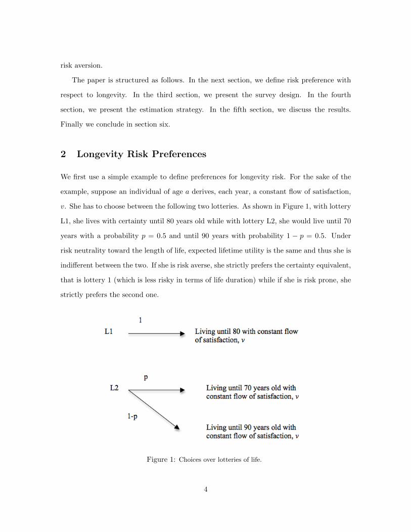
We first use a simple example to define preferences for longevity risk. For the sake of the

example, suppose an individual of age a derives, each year, a constant flow of satisfaction,

v. She has to choose between the following two lotteries. As shown in Figure 1, with lottery

L1, she lives with certainty until 80 years old while with lottery L2, she would live until 70

years with a probability p = 0.5 and until 90 years with probability 1 − p = 0.5. Under

risk neutrality toward the length of life, expected lifetime utility is the same and thus she is

indifferent between the two. If she is risk averse, she strictly prefers the certainty equivalent,

that is lottery 1 (which is less risky in terms of life duration) while if she is risk prone, she

strictly prefers the second one.

Figure 1: Choices over lotteries of life.

4

Let us further define a function G(.) which is an increasing transformation of state

utilities. One simple way to model any attitude toward the risk of longevity of this agent

then consists in making an increasing transformation of state utilities, G(.), such that the

lifetime utility obtained from the lottery L1 is

U(L1) = G((80 − a)v)

and the one obtained from lottery L2 is

U(L2) = 0.5 ×G((70 − a)v) + 0.5 ×G((90 − a)v)

If G′′ = 0, U(L1) = U(L2), and the agent is said to be risk neutral toward the length of life.

If G′′ < 0, U(L1) > U(L2), the agent is risk averse, while if G′′ > 0, U(L2) > U(L1) and

the agent is prone to risk. Yaari (1965) constrains G(.) to be linear. Yet, there is a priori

no reason to believe that agents would be indifferent between these two lotteries of life and

to assume G′′(.) = 0.

3 Survey Design and Data

The simple design in Figure 1 is our starting point. We designed a questionnaire which was

fielded in the RAND American Life Panel (ALP) among panel members which were between

40 and 60 years old at the time of the survey (February 2012). We asked two lottery choice

questions, the first with the parameters of Figure 1 (Q1), the second one (Q3) with more

risk but the same certainty equivalent: 65 and 95 instead of 70 and 90 years old.

For each of these questions, we asked a follow-up question (Q2 and Q4) where we varied

the age in the certainty equivalent scenario, in a table, until the respondent was willing to

switch his answer. For example, suppose the respondent answered he preferred to live for

sure until 80 years old in Q1. Keeping the same risky outcomes (70 or 90 years old), we

ask in Q2 if he would still prefer the certain outcome if he lives to 79, 78, 77 and so on

5

till 71. The age at which the respondent switches his answer identifies an age at which the

respondent is indifferent between the lotteries. As we show below, this allows to estimate

the degree of risk aversion (switching age below). We do something similar for those who

exhibit proneness.

The text of the questions can be found in the appendix. For each question, we stressed

that respondents should assume their standard of living and their health would stay the

same each year. Hence, we assume they enjoy a “constant flow of satisfaction” (equivalently,

their quality of life do not vary) which allows us to focus on risk attitudes toward the length

of life rather than on other forms of time preference or age-dependent utility.4

At first glance, such choice scenarios appear as unrealistic. However, choices over

longevity risks occur in everyday life. For instance, the introduction of a new drug or

the decision to undergo some risky surgery may lead patients to be confronted with com-

parisons between a relatively certain scenario (early death) and an uncertain scenario in

which the drug is effective or not. We decided not to frame the experiment in those terms

to maintain the potential for external validity. From exit interviews of respondents, we got

very few negative comments to these questions which makes us (cautiously) confident that

the questions were salient to the respondents.

Our sample includes of 1425 American respondents between the ages of 40 and 60. In

addition to data from our survey, we also obtain background information from the core

questionnaire of the ALP (gender, income, education, race and ethnicity). The appendix

includes descriptive statistics on the variables we use. The average age of respondents

is 51 years old. A majority (56%) hold a high-school degree, 39.5% a college degree. A

majority, 53.75% earn an income above 50 000$, 25.4% earn between 25 000 and 50 000

dollars. Women account for 60%, blacks for 10% and hispanics for 12%.

4On the definition of a constant flow of satisfaction consumption profile, see Definition 3 in Bommier,2006.

6

4 Estimation

Answers to Q1 and Q3 allow us to compute the fraction of respondents prone, neutral and

averse to risk with respect to length of life. Hence, we can determine the frequency of these

types of behavior. We study the determinants of the probability of being prone, averse or

neutral using a multinomial logit model with socio-economic variables as controls.

We also quantify the extent of risk aversion and proneness for those who were not

indifferent to the two lotteries. Answers to questions Q2 and Q4 define a switching age

ar at which the individual becomes indifferent. This switching age allows to pin down a

measure of risk attitudes toward the length of life, as defined in Bommier (2006).5

Let the age of the respondent be a and X the risk premium the agent is ready to pay

to avoid the risky outcome, measured in life years. This premium is positive for a risk

averse agent and negative for an agent prone to risk. Respondents report in Q2 and Q4 the

certainty equivalent age at which they become indifferent between the lotteries, ar. Hence,

the risk premium is X = 80 − ar for both questions and is implicitly defined by:

G((A− a−X)v) = 0.5G((A− a)v) + 0.5G((A− a)v),

where A = 80, A = 70 and A = 90 in questions Q1-Q2, and A = 80, A = 65 and A = 95

in questions Q3-Q4.

Making a first order Taylor’s expansion around (A− a)v of the LHS and a second order

expansion of the RHS, we can rewrite as:

X + 0.5(A+A− 2A) =(A−A)2 + (A−A)2

4

[− v

G′′((A− a)u)

G′((A− a)v)

].

Define α = −vG′′((A−a)v)G′((A−a)v) as the coefficient of risk aversion with respect to the age at

death A. This coefficient is positive (resp. negative) if the agent is risk averse (resp. prone)

toward the length of life. Thus, one can isolate α of an agent expecting to live (A−a) years

5See definition 2 and equation 4 in Bommier (2006).

7

as follows:

α =4(X + 0.5(A+A− 2A))

(A−A)2 + (A−A)2.

Replacing with the corresponding values of the switching age for Q1 (Q2), we obtain

α =(80 − ar)

50.

For question Q3 (Q4), the expression of for the coefficient has the following expression:

α =4(80 − ar)

450.

Interestingly, these expressions do not depend on v. Using Q2 and Q4, we can thus

compute the degree of risk aversion and risk proneness with respect to the length of life for

each respondent. We can do the same with Q4.

To estimate the determinants of α, we need to deal with right and left-censoring of the

switching age as some respondents never switch. For those choosing the certainty equivalent

(hence being risk averse), let α∗i be the uncensored measure of respondent i and αi,max be

the maximum measure of α if the agent switched at the last age in the list. For those who

chose the risky lottery and never switched in Q2 or Q4, let αi,min be the minimum measure

of α if the agent switched at the last age in that list.

The uncensored measure is a function of characteristics xi (age, income, education, race

and ethnicity) and an unexplained portion εi, normally distributed with variance var(ε):

α∗i = xiβ + εi.

The observed measure, αi, is given by

αi = max(min(αi,max, α∗i ), αi,min).

8

This yields a two-sided tobit model with heterogeneous censoring points. We estimate

parameters β and var(ε) by maximum likelihood.

5 Results

5.1 Frequency of Deviation from Risk Neutrality

Questions Q1 and Q3 allow to quantify the frequency of deviation from risk neutrality. In

Table ??, we report the fraction of respondents choosing the certain lottery (i.e. those who

are risk averse with respect to the length of life), the risky lottery (i.e. the risk-prones) or

who report being indifferent (i.e. the risk-neutrals).

Overall, 73.6% of respondents are not indifferent to the lotteries presented in Q1. Only

26.5% of respondents are risk neutral with respect to the length of life. A slight majority,

38.2% of respondents, are risk averse (they prefer the certainty of living to 80) while 35.4%

are prone to risk (they prefer a 50% chance of living to 70 or 90). There is very little variation

by age in these patterns. However, it appears that those with higher incomes (more than

$50k) and with college degrees are more likely to be averse to the risk of longevity.

When we increase the variance in the second lottery (Q3), more respondents appear to

be risk averse. Almost 60% prefer the certainty of living to 80 while only 19.1% prefer the

risky lottery. A similar income and education gradient is found for question 3.

Next, we investigate how socio-economic characteristics, including race and ethnicity,

affect these answers by estimating a multinomial logit. The reference option is indifference.

Thus we must interpret the estimates relative to this option. Estimates for each question

(Q1 and Q3) along with p-values are reported in Table ??. We do not find an age gradient,

confirming what was reported in Table ??. Income, but not education, appears to increase

the chances of being risk averse with respect to the age at death. Hispanics appear more

likely to report being prone to risk while blacks appear less likely to be risk averse. This

last effect is only statistically significant for Q3. Overall the pattern of estimates is largely

stable across questions. Hence, for other analysis we pool responses to both set of lotteries.

9

% type: Averse Prone Neutral

Question 1total 38.2 35.4 26.5by age

age 40-50 38.1 35.4 26.5age 50-55 37.3 35.2 27.6age 55-60 39.1 35.5 26.4

by incomeless than 25k 24.7 43.2 32.1

25-50k 33.5 39.7 26.8more than 50k 45.4 30.6 24.1

by educationless high school 23.7 45.8 30.5

high school 31.2 40.0 28.8college 49.4 27.9 22.7

Question 3total 59.2 19.1 21.7by age

age 40-50 59.5 19.5 21.0age 50-55 59.1 16.9 24.0age 55-60 58.9 20.7 20.4

by incomeless than 25k 40.8 26.8 32.4

25-50k 55.3 22.9 21.8more than 50k 68.3 14.4 17.4

by educationless high school 45.8 23.7 30.5

high school 51.8 23.9 24.4college 71.1 12.0 17.0

Table 1: Fraction of respondents who prefer certainty equivalent (averse), risky lottery (prone) andare indifferent (neutral). Question 1 offers the choice between living for certain till 80 and a lotterywith equal chances of living till 70 or 90. Question 3 has a risky lottery with equal chances of livingtill 65 or 95.

10

Question 1 Question 3Averse Prone Averse Prone

age 0.001 0.010 -0.010 0.0000.953 0.391 0.391 0.976

high school -0.031 0.010 -0.129 0.3080.936 0.977 0.702 0.428

college 0.534 -0.088 0.374 0.0050.179 0.803 0.292 0.991

25k-50k 0.431 0.131 0.688 0.2510.044 0.501 0.001 0.265

50k more 0.687 0.058 0.975 0.1290.000 0.751 0.000 0.554

male -0.126 -0.024 0.024 -0.0650.370 0.864 0.866 0.706

black -0.251 0.104 -0.509 0.0930.283 0.633 0.019 0.702

hispanic -0.066 0.526 0.099 0.6220.779 0.014 0.664 0.014

intercept -0.296 -0.344 0.796 -0.5580.679 0.620 0.254 0.509

N 1413 1407

Table 2: Multinomial logit parameter estimates with p-values. The reference outcome is riskneutrality. For covariates, the reference category for education is (less than high school), and (lessthan 25k) for income.

11

Before turning to the next section, let us briefly relate our results on the relation between

socio-economic characteristics and risk aversion toward the length of life, with what was

previously found in the literature on standard risk aversion. Barsky et al. (1997) finds that

relative risk aversion is inverse U-shaped in income, age and education. It also finds that

whites are more risk averse than blacks while hispanics are the less risk averse. Arrondel et

al. (2005) using French data, finds that risk aversion is increasing with age but decreasing

in income and in education.6 In both studies, male are found to be less risk averse. These

papers off course, study a different kind of risk aversion, since they are about individual

preferences over monetary risks while our paper focuses on the risk of longevity. Hence,

we find that richer agents are more risk averse toward the length of life while the contrary

is observed for standard risk aversion. Yet, our model yields the same results for the link

between race and risk aversion as the one observed in the case of standard risk aversion.7

5.2 Degree of Deviation from Risk Neutrality

The last section showed some evidence of deviations from neutrality with respect to the

longevity risk. We now analyze the degree of deviation by making use of data on ”switching

ages” to construct the coefficient of risk aversion toward the age at death, α. We pool

answers to both questions Q2 and Q4. We set α = 0 for those who were indifferent between

the two lotteries and compute α for other responses as shown in section 4.

In Figure ??, we report the density of α over both questions Q2 and Q4, excluding

censored observations. Since about one-fourth of respondents were indifferent, there is a

peak at zero. The average estimate of relative risk preference is close to zero (0.009) with

a standard deviation of (0.041). A T-test rejects the null that the mean is zero (t = 9.92).

The distribution is skewed to the left with more mass in the positive domain which reflects

risk aversion toward lenght of life. Note that measures of the risk attitude are strongly

6Kapteyn and Teppa (2011) finds similar results using Dutch data, except for income, which is notsignificant in their study. Yet, they find a negative relation between risk aversion and wealth.

7We do not find any correlation between age and risk aversion, contrary to Barksy et al. (1997), Arrondelet al. (2005) and Kapteyn and Teppa (2011). This may be due to the fact that we restricted the age of oursample to be comprised between 40 and 60.

12

01

02

03

04

0d

en

sity

−.2 −.175 −.15 −.125 −.1 −.075 −.05 −.025 0 .025 .05 .075 .1 .125 .15 .175 .2Risk preference coefficient (mean = 0.009, sd = 0.041)

Figure 2: Distribution of the risk aversion coefficient to both questions Q1 and Q3. Censoredobservations are excluded.

correlated across questions: overall, the correlation coefficient is 0.496 (p < 0.001). If

we focus on respondents who expressed risk aversion in both Q1 and Q3, the correlation

coefficient increases to 0.799 (p < 0.001).

To investigate the correlates of α, we report in Table ?? parameter estimates from

the two-sided tobit model developed in Section 4. Parameter estimates suggest that the

coefficient of risk aversion toward the age at death is positively correlated with income, but

negatively correlated with being black. Age or education does not appear to be correlated

with the risk aversion coefficient.

6 Discussion and Conclusion

In this paper, we test for deviations from risk neutrality toward the length of life. We

designed a questionnaire aimed at detecting and measuring longevity risk aversion. We

present evidence that close to three quarters of respondents do not exhibit risk neutral-

ity toward the length of life (which is typically assumed in intertemporal choice models).

Roughly, three fourth of the population from our survey reported to be either risk averse

13

Estimate P-value

age 0.000 0.471high school -0.006 0.530

college 0.004 0.67625-50k 0.008 0.153

more 50k 0.016 0.001male -0.003 0.384black -.0130 0.032

hispanic -0.002 0.705intercept 0.012 0.511var(ε) 0.007 0.000

N 2433

Table 3: Heterogeneous limit tobit point estimates and p-value.

or risk prone. We found that income was positively correlated with risk aversion but that

neither age nor education had an impact.

This paper provides a first step toward a better understanding of agents’ preferences

toward the length of life. However, there are some limitations to this study. First, we

made the assumption that respondents abstracted from pure time preference considerations

and other time-dependent utility considerations. This allowed us to make the assumption

of constant flow of satisfaction. Some of our results support the view that respondents

abstracted from such considerations for the most part. If only pure time preferences was

at work, impatient agents (i.e. with discount factor less than 1) should always choose the

lottery with no risk. This is clearly not what the results of our survey suggest as we obtain

that a non negligible number of respondents prefer the risky lottery or are indifferent.

Second, empirical evidence has shown that richer agents are more patient, which would

make them choose more often the risky lottery.8 However, we find that richer agents more

often choose the lottery without uncertainty.

One potential extension of the methodology developed is to estimate jointly pure time

preference and longevity risk aversion. In theory, we have two answers to questions with

8For evidence of the relation between time preference and income, see for example Lawrance (1991) andCagetti (2003).

14

different levels of risk. Hence, we have two restrictions as a function of time preference and

the longevity risk aversion coefficient. Hence, it should be possible in theory to disentangle

these effects. This may however be more feasible if we had more rounds of choices among

lotteries.

Second, in a future research project, we will experiment with contextual choice situ-

ations to assess whether respondents are affected by framing effects. For instance, a few

respondents mentioned that it was hard to think about questions on longevity because peo-

ple hardly decide when they die. Also, we realized that we did not asked some questions

which would have been useful for interpreting our results. For example, at question Q.2,

we could not find whether the agents who had not switched at 71 years old would have

effectively switched at 70, simply because we did not ask this last question. As a result, we

could not find whether these agents did not understand the question.

Other than these limitations, one obvious conclusion of this pilot project is that it

appears to be possible to ask respondents such questions about the risk over the length of

life. As Bommier and Villeneuve (2012) mention in the conclusion of their paper, ”the key

issue is therefore to estimate is to estimate mortality risk aversion. The difficulty of the task

should not be underestimated. (...) This should be rather seen as a long-term objective

that will probably require the collection of specific data”.

15

References

[1] Aldy, J. E., and W. K. Viscusi, 2003. Age variations in workers value of statistical life.

NBER Working paper No. 10199.

[2] Arrondel,L., Masson A. and D. Verger, 2004. Mesurer les prfrences individuelles lgard

du risque, conomie et statistique, n 374-375, 53-85.

[3] Barsky, R., T. Juster, K. Miles and M. Shapiro, 1997. Preference parameters and

behavioral heterogeneity: An experimental approach in the Health and Retirement

Study, The Quarterly Journal of Economics, 112(2), In Memory of Amos Tversky

(1937-1996), 537-579.

[4] Bommier, A., 2006. Uncertain lifetime and intertemporal choice: risk aversion as a

rationale for time discounting. International Economic Review, 47(4), 1223-1246.

[5] Bommier, A., M-L. Leroux and J-M. Lozachmeur, 2011a. On the public economics of

annuities with differential mortality. Journal of Public Economics, 95(7-8), 612-623.

[6] Bommier, A., M-L. Leroux and J-M. Lozachmeur, 2011b. Differential mortality and

social security. Canadian Journal of Economics, 44(1), 273-289.

[7] Bommier, A. and F. Le Grand, 2012. Too Risk Averse to Purchase Insurance? A

Theoretical Glance at the Annuity Puzzle. ETH Risk Center WP Series ETH-RC-12-

002.

[8] Bommier, A. and B. Villeneuve, 2012. Risk aversion and the value of risk to life. Journal

of Risk and Insurannce, 79(1), 77-103.

[9] Cagetti, M., 2003. Wealth Accumulation Over the Life Cycle and Precautionary Sav-

ings. Journal of Business and Economic Statistics, 21(3), 339-353.

[10] Calvo, G.A., and M. Obstfeld, 1988. Optimal time-consistent fiscal policy with finite

lifetimes. Econometrica 56, 41132.

16

[11] Diamond, P.A., ed., 2003. Models of optimal retirement incentives with varying life

expectancies. In “Taxation, Incomplete Markets and Social Security”, chapter 7 (Cam-

bridge, MA: MIT Press).

[12] Fleurbaey, M., Leroux, M-L. and Ponthiere, G., 2010. Compensating the dead? Yes

we can! CORE Discussion Paper 2010-66.

[13] Kapteyn A., and F. Teppa, 2011. Subjective measures of risk aversion, fixed costs, and

portfolio choice, Journal of Economic Psychology, 32, 564580.

[14] Kihlstrom, R.E., Mirman, L.J., 1974. Risk aversion with many commodities. Journal

of Economic Theory 8, 361-388.

[15] Leroux M-L., Pestieau P., Ponthire G., 2011. Longevity, genes and efforts: an optimal

taxation approach to prevention. Journal of Health Economics, 30(1), 62-76.

[16] Lawrance, E.C., 1991. Poverty and the Rate of Time Preference: Evidence from Panel

Data. Journal of Political Economy, 99(1), 54-77.

[17] Yaari, M., 1965. Uncertain lifetime, life insurance and the theory of the consumer. The

Review of Economic Studies 32 (2), 137150

17

Survey Questionnaire

Respondents were asked the following first question:9

Q1: In the following scenarios, imagine that your standard of living and your healthcondition are preserved no matter how long you live. Please choose between the followingoptions:

1) Live till you are 80 years old.2) A 50% chance of living till you are 70 years old and a 50% chance of living till you

are 90 years old.3) You are indifferent between options 1 and 2.

If at this question Q1, they answered 1, they were asked Q2.1; if they answered 2, theywere asked Q2.2 and if they had answered 3, they were asked Q2.3. These questions arereported below.

Q2.1: In the previous question, you preferred option 1 (you live till you are 80 yearsold) to option 2 (a 50% chance you live till 70 years old and a 50% chance till 90 years old).

Suppose now that we modify option 1 and keep option 2 the same. For the followingpossibilities, please indicate whether you still prefer the modified option 1 if you live tillyou are

Preferred Not preferred Indifferent

a) 79 years oldb) 78 years oldc) 77 years oldd) 76 years olde)75 years oldf) 74 years oldg) 73 years oldh) 72 years oldi) 71 years old

Note that only one answer at each line was possible.

Q2.2: In the previous question you preferred option 2 (a 50% chance you live till 70years old and a 50% chance till 90 years old) to option 1 (you live till you are 80 years old).Suppose now that we modify option 1 and keep option 2 the same. For the following

9Note that agents could go back.

18

possibilities, please indicate whether you still prefer option 2 to living till you are

Preferred Not preferred Indifferent

a) 81 years oldb) 82 years oldc) 83 years oldd) 84 years olde)85 years oldf) 86 years oldg) 87 years oldh) 88 years oldi) 89 years old

We further asked a second identical set of questions except for the variance of theuncertain lottery:

Q3: In the following scenarios, imagine that your standard of living and your healthcondition are preserved no matter how long you live. Please choose between the followingoptions:

1) Live till you are 80 years old.2) A 50% chance of living till you are 65 years old and a 50% chance of living till you

are 95 years old.3) You are indifferent between options 1 and 2.

Depending on what agents answered at question Q.3, we asked a second question, Q4.1identical to question Q2.1 and Q4.2 identical to Q2.2.

19