J. Earth Syst. Sci. (2017) 126:106 c© Indian Academy of SciencesDOI 10.1007/s12040-017-0884-1

Evidence of topographic disequilibrium in the SubarnarekhaRiver Basin, India: A digital elevation model based analysis

Shantamoy Guha1,* and Priyank Pravin Patel2

1Earth Sciences Discipline, Indian Institute of Technology, Gandhinagar 382 355, India.2Department of Geography, Presidency University, Kolkata 700 073, India.*Corresponding author. e-mail: shantamoy.guha@iitgn.ac.in

MS received 29 January 2017; accepted 20 April 2017; published online 16 October 2017

Cratonic areas experience complex process-response changes due to their operative endogenic andexogenic forces varying in intensity and spatiality over long timescales. Unlike zones of active deformation,the surface expression of the transient signals in relatively tectonically stable areas are usually scant.The Subarnarekha River Basin, in eastern India, is a prime example of a Precambrian cratoniclandscape, overlain in places by Tertiary and Quaternary deposits. A coupled quantitative-qualitativeapproach is employed towards deciphering tectonic and geological influences across linear and arealaspects, at the basin and sub-basin scale. Within this landscape, the transient erosional signatures areexplored, as recorded in the disequilibrium conditions of the longitudinal profiles of the major streams,which are marked by a number of waterfalls at structural and lithological boundaries. Mathematicalexpressions derived from the normalized longitudinal profiles of these streams are used to ascertaintheir stage of development. Cluster analysis and chi plots provide significant interpretations of the roleof vertical displacements or litho-structural variations within the basin. These analyses suggest that aheterogeneous, piece-meal response to the ongoing deformation exists in the area, albeit, determiningthe actual rate of this deformation or its temporal variation is difficult without correlated chronologicaldatasets.

Keywords. Neotectonics; longitudinal profile; DEM; morphometry; geological structure; streamresponse.

1. Introduction

Landforms are the product of the coupling betweentectonic and denudational processes. Tectonic for-ces change the relative elevation of the surface,thereby increasing the potential energy for ero-sion (England and Molnar 1990), and also exertan influence on the magnitude and intensity of

Supplementary material pertaining to this article is available on the Journal of Earth System Science website (http://www.ias.ac.in/Journals/Journal of Earth System Science).

denudation (Thornbury 1954). Lithological andstructural characteristics provide a template togauge the effectiveness of these erosional process,e.g., that of a river either at the basin scale (Nagand Chakraborty 2003), or at the reach scale(Strecker et al. 2003), and furthermore, can them-selves be discerned from the nature of erosionalactivity that has occurred (Duncan et al. 2003;

1

106 Page 2 of 20 J. Earth Syst. Sci. (2017) 126:106

Ahmadi et al. 2006). However, quantitative insightinto the interaction between tectonics and erosionalprocesses in the context of geologic and structuralformations is scant and poorly understood in termsof the resultant topography (Burbank et al. 1996).

Traditionally, cratonic areas or ‘Shields’ havebeen considered to be stable enough to showcaseprominent effects of neotectonics (Valdiya 2001;Sangode et al. 2013). However, transient character-istics are conspicuous in many parts of the worldunderlain by old and relict topography (Princeet al. 2011; Mandal et al. 2015). The Singhbhumcraton, in eastern India, portrays similar transientcharacteristics in the form of knickpoints alongthe longitudinal courses of many streams coursingthrough it, albeit it has been only accounted forPrecambrian tectonics, due to its long and complexevolutionary history (Sarkar 1982; Saha 1994). Toinvestigate the tectonic inference from the terrain,it is paramount that tectonic indices be also cou-pled with the corresponding litho-structural settingof the area (Lima and Binda 2013; Azanon et al.2015).

In this study, we attempt to identify the tectonicand structural controls on river channel form in theSubarnarekha River Basin (prominently underlainby Precambrian rocks of the Singhbhum craton)via geomorphic and morphometric analysis. A dualframework has thus been used in this study, incor-porating qualitative methods to decipher the exis-tent geologic and structural influences, alongsidequantitative measures for ascertaining probabletectonic effects on the longitudinal channel profiledevelopment. Qualitative measures include iden-tification of knickpoints using a digital elevationmodel and correlating it with the bedrock geol-ogy and structure. Quantitative measures involveenumeration and mapping of selected indices ofactive tectonics for the studied Subarnarekha RiverBasin.

2. Study area

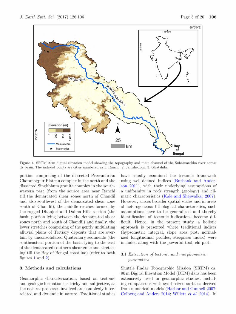
Draining a catchment area of approximately 19,000km2, the River Subarnarekha is an important east-ward flowing river in eastern India. It rises nearNagri village (23◦18’N, 85◦11’E), just north ofRanchi (major city #1 in figure 1) at an eleva-tion of ∼610 m in the Ranchi district of Jharkhand,drains the southeastern portion of the Chotanag-pur Plateau, cuts through the Dalma Hill Rangeat Chandil (22◦54’N, 86◦02’E), just upstream ofJamshedpur (major city #2 in figure 1) and

debouches into the Bay of Bengal at Talshari(21◦33’N, 87◦23’E) in the Baleswar district ofOrissa, after traversing a distance of about 395 km.

The prominent hill ranges within this basin aresituated above an average elevation of 450m fromthe mean sea level, and are flanked by prominentdenudational scarps situated at elevations of 300–450 m (figure 1). The Dalma Range stands withinthis landscape and the presence of lateritic duri-crust at altitudes of 600 and 900m are thought torepresent two uplifted palaeo-surfaces (Mahadevan2002). A major portion of the total basin area liesbelow 300 m (∼80%), incorporating the undulat-ing plains of the lower reaches of the rivers thathave their sources in the above hills, and which areherein overlain by considerable floodplain deposits(figure 1).

The entire basin can be subdivided into threebroad geological units, i.e., Archaean–Precambrianformations, Tertiary formations and Quaternaryalluvium. Considerable portions of the upper andmiddle basin areas are underlain by exposed Pre-cambrian metamorphic and igneous rocks. In itslower reaches, the main Subarnarekha River chan-nel interacts with younger formations as well aswith the unconsolidated deposits of Tertiary andQuaternary sediments (figure 2). South of theDalma Range, the ridges of the Singhbhum ShearZone (SSZ) splay arcuately along the west bankof the Subarnarekha’s course, being dissected bythe river at Chandil and go on to form sharpbends further east (figure 2). Rejuvenations ofstreams adjacent to and within the SSZ have beenreported, caused by surficial movements on a minorscale, and accounted for by the low seismic sig-natures recorded in this area (Banerji et al. 1970;Mukhopadhyay 1977; Mahadevan 2002).

The average annual rainfall within the basinranges between 1100 and 1400mm (figure 3) (Chat-terjee et al. 2014), with this amount being receivedalmost entirely during the monsoonal months ofJune–September, as is reflected in the strongly lep-tokurtic nature of the stream flow hydrographs ofthe rivers (Yarrakula et al. 2010). In addition tothese, the Subarnarekha is also a major transporterof heavy metals from its upstream region (Giriet al. 2013), with significant mineral resources andmining centers being located along its course, par-ticularly in the vicinity of Ghatshila (major city#3 in figure 1).

Using a combination of the principal geologicand geomorphologic units, the basin terrain canbe divided into three broad units, i.e., the upper

J. Earth Syst. Sci. (2017) 126:106 Page 3 of 20 106

Figure 1. SRTM 90 m digital elevation model showing the topography and main channel of the Subarnarekha river acrossits basin. The indexed points are cities numbered as 1: Ranchi, 2: Jamshedpur, 3: Ghatshila.

portion comprising of the dissected PrecambrianChotanagpur Plateau complex in the north and thedissected Singhbhum granite complex in the south-western part (from the source area near Ranchitill the demarcated shear zones north of Chandiland also southwest of the demarcated shear zonesouth of Chandil), the middle reaches formed bythe rugged Dhanjori and Dalma Hills section (thebasin portion lying between the demarcated shearzones north and south of Chandil) and finally, thelower stretches comprising of the gently undulatingalluvial plains of Tertiary deposits that are over-lain by unconsolidated Quaternary sediments (thesoutheastern portion of the basin lying to the eastof the demarcated southern shear zone and stretch-ing till the Bay of Bengal coastline) (refer to bothfigures 1 and 2).

3. Methods and calculations

Geomorphic characterization, based on tectonicand geologic formations is tricky and subjective, asthe natural processes involved are complexly inter-related and dynamic in nature. Traditional studies

have usually examined the tectonic frameworkusing well-defined indices (Burbank and Ander-son 2011), with their underlying assumptions ofa uniformity in rock strength (geology) and cli-matic characteristics (Kale and Shejwalkar 2007).However, across broader spatial scales and in areasof heterogeneous lithological characteristics, suchassumptions have to be generalized and therebyidentification of tectonic indications become dif-ficult. Hence, in the present study, a holisticapproach is presented where traditional indices(hypsometric integral, slope area plot, normal-ized longitudinal profiles, steepness index) wereincluded along with the powerful tool, chi plot.

3.1 Extraction of tectonic and morphometricparameters

Shuttle Radar Topographic Mission (SRTM) ca.90m Digital Elevation Model (DEM) data has beenextensively used in geomorphic studies, includ-ing comparisons with synthesized surfaces derivedfrom numerical models (Harbor and Gunnell 2007;Colberg and Anders 2014; Willett et al. 2014). In

106 Page 4 of 20 J. Earth Syst. Sci. (2017) 126:106

87°0'0"E

22°0

'0"N

25km

H

J

D

Dalm a Hills

H- Hundru, J- Johna, D- Dassam

waterfalls

Shear zonesStream

GeologyBasics and Ultrabasics rocks

Chotanagpur Gneiss

Dhanjori Quartzite and Conglomerate

Metavolcanics / Metasediments

Older alluvium and Laterite

Pleistocene sediments

Proterozoic metasediment

Singhbhum Granite

Singhbhum Metasediment

Tertiary Sediment

Basics and Dolerite

Danjori/Dalma Basics

Chandil

Figure 2. Bedrock geology and shear zones (after Geological Survey of India) within the Subarnarekha basin, overlain by adetailed drainage map.

the present study, therefore, SRTM DEM is usedto derive the tectonic indices for the SubarnarekhaRiver basin. For identifying the regional patternsof these indices, the main basin has furthermorebeen divided into 12 sub-basins using the Soil andWater Analysis (SWAT) model (Gassman et al.2007), using specified stream junction points. Mat-lab based Geomorphtools (Whipple et al. 2007) andTopoToolbox (Schwanghart and Kuhn 2010) havebeen used to calculate most of the tectonic andmorphometric indices. To analyze the longitudinalprofiles, we have extracted the principal stream andits tributaries by manual pour point.

3.2 Plotting normalized longitudinal profiles withbest-fit curves

Although the breaks in a river’s longitudinal pro-file (i.e., an abrupt channel elevation or channelslope change) are prime indicators of structuraland lithological alterations across its course, themarked difference of magnitude between thesechanges, i.e., that of the elevation difference froma river’s source to its mouth (its fall) vs. that of

its entire channel length from the source to mouth,introduces the problem of scaling both these vari-ables (Lee and Tsai 2010). In order to nullify thisscaling factor, a normalization procedure has beenapplied to the main channel, as well as to theexamined tributaries by manual pour point selec-tion method (see supplementary figure S2 for thewatersheds delineation). Four mathematical func-tions were used to compare and derive a best-fitcurve on the respective profiles to ascertain thestage of development of the respective basins, aswell as inculcate a process-based understanding.These are as follows:

The linear function, y = ax + b, (1)The exponential function, y = aebx, (2)The logarithmic function, y = a lnx + b, (3)The power regression model, y = axb, (4)

In these equations, y is the elevation (it is cal-culated as h/h0; h is the elevation of each point,h0 is the elevation of the source), x is the lengthof the river (l/l0; l is the distance of any discrete

J. Earth Syst. Sci. (2017) 126:106 Page 5 of 20 106

87°0'0"E

22°0

'0"N

25km

Average Annual Rainfall (mm/year)

2,001 - 2,5001,501 - 2,000

489 - 1,000 1,001 - 1,500

2,501 - 3,500

Subarnarekha basin

Subarnarekha main stream

Figure 3. Annual average rainfall distribution over Subarnarekha River basin. Rainfall data after Bookhagen and Strecker(2008) and Bookhagen and Burbank (2010). The precipitation data is resampled TRMM 2B31 v6 product of 5 km spatialresolution and obtained from http://www.geog.ucsb.edu/∼bodo/TRMM/.

point from the source, l0 is the total length of thestream), while a and b are coefficients.

3.3 Extracting concavity and steepness indices

The combination of the conservation of mass state-ment along with the bed shear stress model can bereproduced as the following equation (Howard andKerby 1983; Howard 1994):

∂z

∂t= U (x, t) − K (x, t)A (x, t)m

∣∣∣∣

∂z

∂x

∣∣∣∣

n

. (5)

It is assumed that the topography is in a steadystate, i.e., the rate of uplift is balanced by theerosion process (∂z/∂t = 0) (Whipple and Tucker1999; Whipple et al. 2007). Equation (5) then canbe written as:

∣∣∣∣

dz

dx

∣∣∣∣=

(U

K

)1/n

A (x)−m/n , (6)

or

S = ksA−θ (7)

where the local channel slope is represented asS, A is the upstream drainage area, and ks andθ are referred to as the steepness and concavityindices, respectively. Therefore, there is an inher-ent power law relationship between the channelslope and the drainage area (Flint 1974). Thisrelationship is used in the present study by cal-culating the normalized steepness index (ksn) andthe concavity index (θ), for the main stream flow-ing through the entire Subarnarekha basin aswell as for the principal streams of each of thesub-basins.

The longitudinal profiles of the main river andits principal tributaries, along with the geologicformations over which they propagate, have beenconsidered while analyzing the geologic constraintsand influences apparent in the development ofthese profiles. The principal and tributary streamcourses are used for extraction of slope-area plotsto estimate the normalized steepness index (ksn)and the concavity index (θ), with the referenceconcavity (θref), using the help of geomorphtools

106 Page 6 of 20 J. Earth Syst. Sci. (2017) 126:106

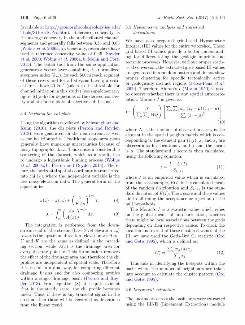
(available at http://geomorphtools.geology.isu.edu/Tools/StPro/StPro.htm). Reference concavity isthe average concavity in the undistributed channelsegments and generally falls between 0.35 and 0.65(Wobus et al. 2006a, b). Generally, researchers haveused a reference concavity value of 0.45 (Snyderet al. 2000; Wobus et al. 2006a, b; Molin and Corti2015). The batch tool from the same applicationgenerates a vector layer containing the normalizedsteepness index (ksn), for each 500m reach segmentof these rivers and for all streams having a criti-cal area above 20 km2 (taken as the threshold forchannel initiation in this study) (see supplementaryfigure S1(a–h) for depictions of the derived concav-ity and steepness plots of selective sub-basins).

3.4 Deriving the chi plots

Using the algorithm developed by Schwanghart andKuhn (2010), the chi plots (Perron and Royden2013), were generated for the main stream as wellas for its tributaries. Traditional slope-area plotsgenerally have numerous uncertainties because ofnoisy topographic data. This causes a considerablescattering of the dataset, which as a result, hasto undergo a logarithmic binning process (Wobuset al. 2006a, b; Perron and Royden 2013). There-fore, the horizontal spatial coordinate is transferredinto chi (χ), where the independent variable is theless noisy elevation data. The general form of theequation is:

z (x) = z (xb) +(

U

KAo

)1/n

χ, (8)

χ =∫ x

xb

(Ao

A (x)

)m/n

dx. (9)

The integration is performed from the down-stream end of the stream (base level elevation xb)towards the upstream direction (elevation x). Here,U and K are the same as defined in the preced-ing section, while A(x) is the drainage area forevery discrete point x. This formulation removesthe effect of the drainage area and therefore the chiprofiles are independent of spatial scale. Thereforeit is useful in a dual way, for comparing differentdrainage basins and for also comparing profileswithin a single drainage basin (Perron and Roy-den 2013). From equation (8), it is quite evidentthat in the steady state, the chi profile becomeslinear. Thus, if there is any transient signal in theerosion, then these will be recorded as deviationsfrom the linear trend.

3.5 Hypsometric analysis and statisticalderivations

We have also prepared grid-based HypsometricIntegral (HI) values for the entire watershed. Thesegrid-based HI values provide a better understand-ing for differentiating the geologic imprints andtectonic processes. However, without proper statis-tical conversion, the extracted grid-based HI valuesare generated in a random pattern and do not showproper clustering for specific tectonically activeor geologically distinct regions (Perez-Pena et al.2009). Therefore, Moran’s I (Moran 1950) is usedto observe whether there is any spatial autocorre-lation. Moran’s I is given as:

I=

(

N∑

i

∑

j Wij

) [∑

i

∑

i wij (xi − μ) (xj − μ)∑

i (xi − μ)2

]

(10)

where N is the number of observations, wij is theelement in the spatial weights matrix which is cor-responding to the element pair (i , j ), x i and xj areobservations for locations i and j and the meanis μ. The standardized z score is then calculatedusing the following equation:

z =I − E (I)

SE(I)(11)

where I is an empirical value which is calculatedfrom the total sample, E(I) is the calculated meanof the random distribution and SE(I) is the stan-dard deviation of E(I). The z score and the p valuesaid in affirming the acceptance or rejection of thenull hypothesis.

The Moran’s I is a statistic value which relieson the global means of autocorrelation, whereasthere might be local associations between the gridsdepending on their respective values. To check thelocation and extent of these clustered values of theHI, we have used the Getis-Ord Gi statistic (Ordand Getis 1995), which is defined as:

G∗i =

∑

j wij (d)xj∑

j xj(12)

This aids in identifying the hotspots within thebasin where the number of neighbours are takeninto account to calculate the cluster pattern (Ordand Getis 1995).

3.6 Lineament extraction

The lineaments across the basin area were extractedusing the LINE (Lineament Extraction) module

J. Earth Syst. Sci. (2017) 126:106 Page 7 of 20 106

available for this purpose in PCI Geomatica (Kocalet al. 2007; Geomatics 2015). The six inputsrequired to extract the lineaments are respec-tive values for the Radius of filter (in pixels),the Threshold for edge gradient, the Thresholdfor curve length, the Threshold for line fittingerror, the Threshold for angular difference and theThreshold for linking distance parameters (Abdul-lah and Abdoh 2013; Geomatics 2015). The valueswere input following the different threshold val-ues as suggested by Prasad et al. (2013), Rajand Ahmed (2014) and Shankar et al. (2016). Thederived curvilinear features were then converted tovectors that were overlain on Google Earth imageryfor visual comparison based accuracy assessment,suitably modified thereafter and finally extractedafter such confirmation. These were clipped usinga mesh of 1 km2 grids overlain over the basin andtheir density in each grid enumerated for eventualisopleth mapping.

4. Results and discussion

4.1 Concavity and steepness indices

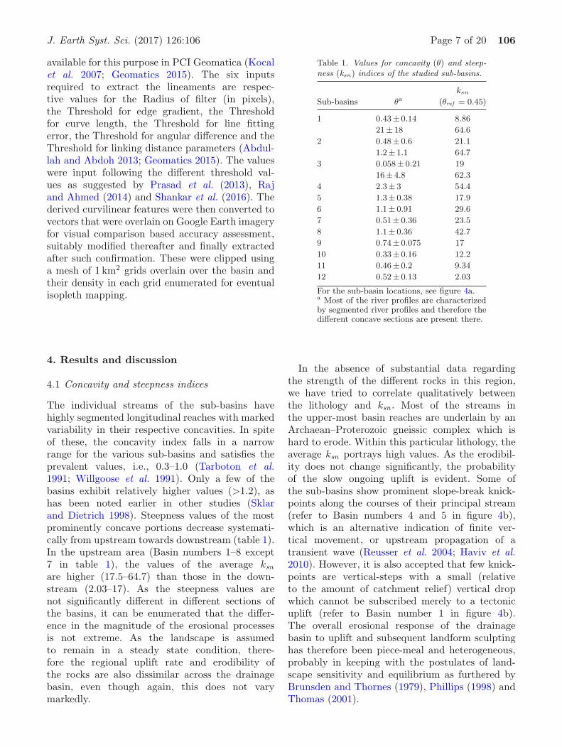
The individual streams of the sub-basins havehighly segmented longitudinal reaches with markedvariability in their respective concavities. In spiteof these, the concavity index falls in a narrowrange for the various sub-basins and satisfies theprevalent values, i.e., 0.3–1.0 (Tarboton et al.1991; Willgoose et al. 1991). Only a few of thebasins exhibit relatively higher values (>1.2), ashas been noted earlier in other studies (Sklarand Dietrich 1998). Steepness values of the mostprominently concave portions decrease systemati-cally from upstream towards downstream (table 1).In the upstream area (Basin numbers 1–8 except7 in table 1), the values of the average ksn

are higher (17.5–64.7) than those in the down-stream (2.03–17). As the steepness values arenot significantly different in different sections ofthe basins, it can be enumerated that the differ-ence in the magnitude of the erosional processesis not extreme. As the landscape is assumedto remain in a steady state condition, there-fore the regional uplift rate and erodibility ofthe rocks are also dissimilar across the drainagebasin, even though again, this does not varymarkedly.

Table 1. Values for concavity (θ) and steep-ness (ksn) indices of the studied sub-basins.

ksn

Sub-basins θa (θref = 0.45)

1 0.43 ± 0.14 8.86

21 ± 18 64.6

2 0.48 ± 0.6 21.1

1.2 ± 1.1 64.7

3 0.058 ± 0.21 19

16 ± 4.8 62.3

4 2.3 ± 3 54.4

5 1.3 ± 0.38 17.9

6 1.1 ± 0.91 29.6

7 0.51 ± 0.36 23.5

8 1.1 ± 0.36 42.7

9 0.74 ± 0.075 17

10 0.33 ± 0.16 12.2

11 0.46 ± 0.2 9.34

12 0.52 ± 0.13 2.03

For the sub-basin locations, see figure 4a.a Most of the river profiles are characterizedby segmented river profiles and therefore thedifferent concave sections are present there.

In the absence of substantial data regardingthe strength of the different rocks in this region,we have tried to correlate qualitatively betweenthe lithology and ksn . Most of the streams inthe upper-most basin reaches are underlain by anArchaean–Proterozoic gneissic complex which ishard to erode. Within this particular lithology, theaverage ksn portrays high values. As the erodibil-ity does not change significantly, the probabilityof the slow ongoing uplift is evident. Some ofthe sub-basins show prominent slope-break knick-points along the courses of their principal stream(refer to Basin numbers 4 and 5 in figure 4b),which is an alternative indication of finite ver-tical movement, or upstream propagation of atransient wave (Reusser et al. 2004; Haviv et al.2010). However, it is also accepted that few knick-points are vertical-steps with a small (relativeto the amount of catchment relief) vertical dropwhich cannot be subscribed merely to a tectonicuplift (refer to Basin number 1 in figure 4b).The overall erosional response of the drainagebasin to uplift and subsequent landform sculptinghas therefore been piece-meal and heterogeneous,probably in keeping with the postulates of land-scape sensitivity and equilibrium as furthered byBrunsden and Thornes (1979), Phillips (1998) andThomas (2001).

106 Page 8 of 20 J. Earth Syst. Sci. (2017) 126:106

a

b

Figure 4. Longitudinal profiles and concavity analysis (a) Sub-basins that are demarcated with SWAT tool. (b) Longitudinalprofiles and slope area plots for selected sub-basins. The basin number is denoted on the left-hand side of each sub-plots.The slope is calculated from a contour interval of 20 m.

J. Earth Syst. Sci. (2017) 126:106 Page 9 of 20 106

a

b

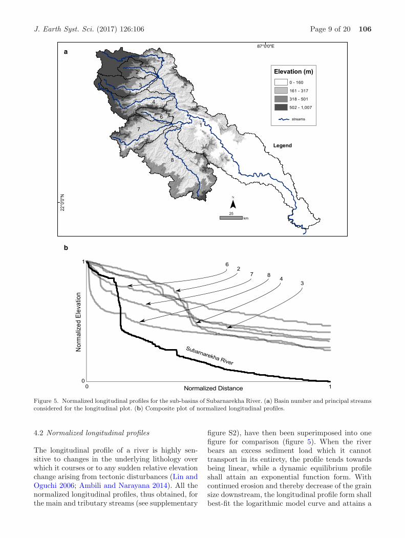
Figure 5. Normalized longitudinal profiles for the sub-basins of Subarnarekha River. (a) Basin number and principal streamsconsidered for the longitudinal plot. (b) Composite plot of normalized longitudinal profiles.

4.2 Normalized longitudinal profiles

The longitudinal profile of a river is highly sen-sitive to changes in the underlying lithology overwhich it courses or to any sudden relative elevationchange arising from tectonic disturbances (Lin andOguchi 2006; Ambili and Narayana 2014). All thenormalized longitudinal profiles, thus obtained, forthe main and tributary streams (see supplementary

figure S2), have then been superimposed into onefigure for comparison (figure 5). When the riverbears an excess sediment load which it cannottransport in its entirety, the profile tends towardsbeing linear, while a dynamic equilibrium profileshall attain an exponential function form. Withcontinued erosion and thereby decrease of the grainsize downstream, the longitudinal profile form shallbest-fit the logarithmic model curve and attains a

106 Page 10 of 20 J. Earth Syst. Sci. (2017) 126:106

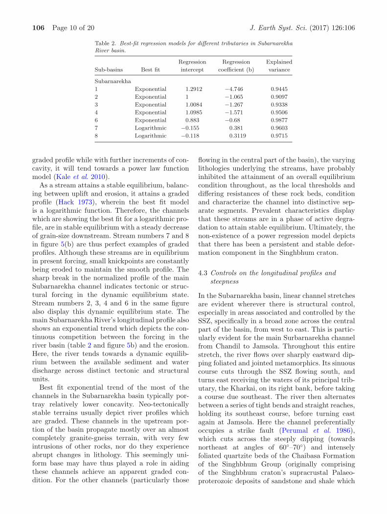
Table 2. Best-fit regression models for different tributaries in SubarnarekhaRiver basin.

Regression Regression Explained

Sub-basins Best fit intercept coefficient (b) variance

Subarnarekha

1 Exponential 1.2912 −4.746 0.9445

2 Exponential 1 −1.065 0.9097

3 Exponential 1.0084 −1.267 0.9338

4 Exponential 1.0985 −1.571 0.9506

6 Exponential 0.883 −0.68 0.9877

7 Logarithmic −0.155 0.381 0.9603

8 Logarithmic −0.118 0.3119 0.9715

graded profile while with further increments of con-cavity, it will tend towards a power law functionmodel (Kale et al. 2010).

As a stream attains a stable equilibrium, balanc-ing between uplift and erosion, it attains a gradedprofile (Hack 1973), wherein the best fit modelis a logarithmic function. Therefore, the channelswhich are showing the best fit for a logarithmic pro-file, are in stable equilibrium with a steady decreaseof grain-size downstream. Stream numbers 7 and 8in figure 5(b) are thus perfect examples of gradedprofiles. Although these streams are in equilibriumin present forcing, small knickpoints are constantlybeing eroded to maintain the smooth profile. Thesharp break in the normalized profile of the mainSubarnarekha channel indicates tectonic or struc-tural forcing in the dynamic equilibrium state.Stream numbers 2, 3, 4 and 6 in the same figurealso display this dynamic equilibrium state. Themain Subarnarekha River’s longitudinal profile alsoshows an exponential trend which depicts the con-tinuous competition between the forcing in theriver basin (table 2 and figure 5b) and the erosion.Here, the river tends towards a dynamic equilib-rium between the available sediment and waterdischarge across distinct tectonic and structuralunits.

Best fit exponential trend of the most of thechannels in the Subarnarekha basin typically por-tray relatively lower concavity. Neo-tectonicallystable terrains usually depict river profiles whichare graded. These channels in the upstream por-tion of the basin propagate mostly over an almostcompletely granite-gneiss terrain, with very fewintrusions of other rocks, nor do they experienceabrupt changes in lithology. This seemingly uni-form base may have thus played a role in aidingthese channels achieve an apparent graded con-dition. For the other channels (particularly those

flowing in the central part of the basin), the varyinglithologies underlying the streams, have probablyinhibited the attainment of an overall equilibriumcondition throughout, as the local thresholds anddiffering resistances of these rock beds, conditionand characterize the channel into distinctive sep-arate segments. Prevalent characteristics displaythat these streams are in a phase of active degra-dation to attain stable equilibrium. Ultimately, thenon-existence of a power regression model depictsthat there has been a persistent and stable defor-mation component in the Singhbhum craton.

4.3 Controls on the longitudinal profiles andsteepness

In the Subarnarekha basin, linear channel stretchesare evident wherever there is structural control,especially in areas associated and controlled by theSSZ, specifically in a broad zone across the centralpart of the basin, from west to east. This is partic-ularly evident for the main Surbarnarekha channelfrom Chandil to Jamsola. Throughout this entirestretch, the river flows over sharply eastward dip-ping foliated and jointed metamorphics. Its sinuouscourse cuts through the SSZ flowing south, andturns east receiving the waters of its principal trib-utary, the Kharkai, on its right bank, before takinga course due southeast. The river then alternatesbetween a series of tight bends and straight reaches,holding its southeast course, before turning eastagain at Jamsola. Here the channel preferentiallyoccupies a strike fault (Perumal et al. 1986),which cuts across the steeply dipping (towardsnortheast at angles of 60◦–70◦) and intenselyfoliated quartzite beds of the Chaibasa Formationof the Singhbhum Group (originally comprisingof the Singhbhum craton’s supracrustal Palaeo-proterozoic deposits of sandstone and shale which

J. Earth Syst. Sci. (2017) 126:106 Page 11 of 20 106

Figure 6. Longitudinal profile superimposed on the lithology and the structure. Average ksn values for the respectivesegments is also plotted on the same.

were metamorphosed into the present quartzite andmica-schist – Mazumder et al. 2012), into whichthe river duly incises, becoming deeply entrenchedand narrowing considerably, while folds, plungingto the northeast, are also present along the banks,through which the river has carved its course (Rao1962). This not only demonstrates the superposednature of the main channel, but also how struc-tural and lithologic variations have influenced thechannel character herein.

In order to identify the role of surface lithologyon the long profile development, we have super-imposed the drainage lines and associated breakin profiles over surface lithology (figure 6). Knick-points, once formed, tend to migrate upstream bycontinual recession (Whipple and Tucker 1999). Adistinct possibility behind the minor displacementof these knickpoints from the nearby litho-structural boundaries may therefore be the knick-point migration process. Only the Johna Falls onthe Gunga River coincides with the transition zonebetween the gneissic and ultra-basic rocks (figure 2,marked as J). However, the absence of observablelithological changes at the site may be ascribedto the aforesaid migration process. The other twomighty waterfalls in the upper portion of thebasin do not coincide with any distinct lithologicaltransition zone (figure 2 – Hundru Falls (markedH) on the Subarnarekha River and the Dassam

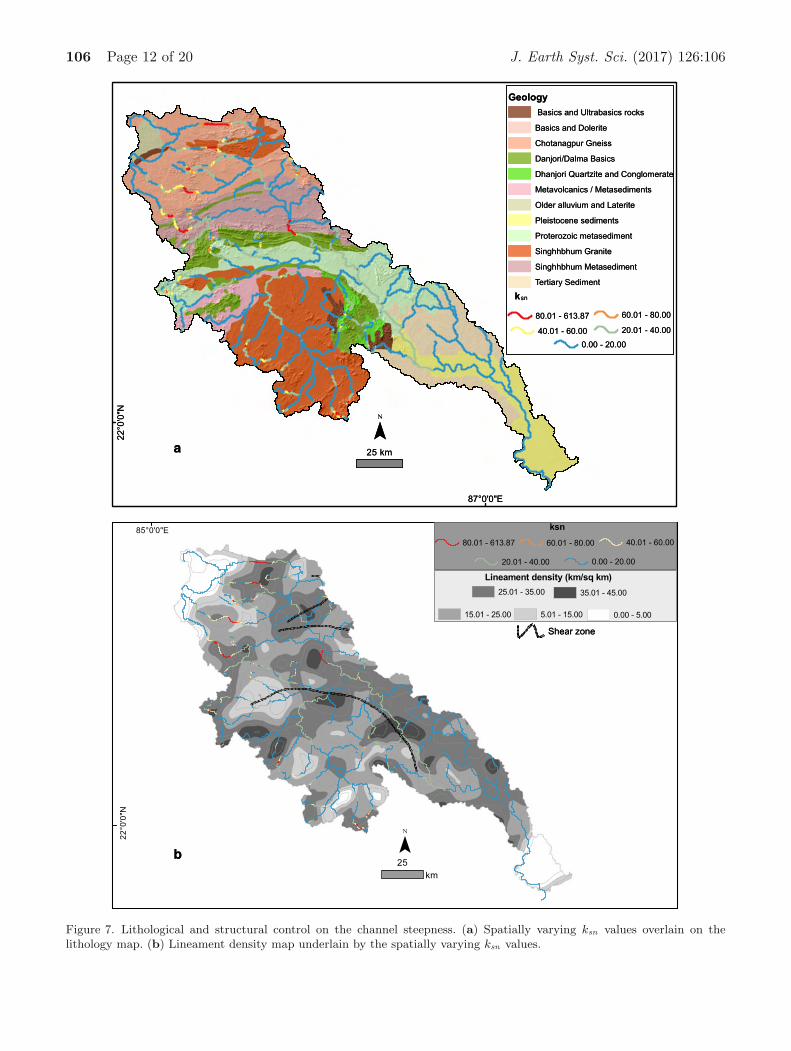
Falls (marked D) on the Kanchi River). Planformobservations of channel steepness from figure 7(a)reveals that the lithological transitions are notalways associated with high ksn values. The lowerksn value segments are primarily present in threelocales – in the gently undulating piedmont zoneadjacent to the dissected plateau tract in the north,within the southern extents of the Kharkai River’ssub-basin in the south-central part over a homo-geneous lithology of Singhbhum granite and acrossthe Quaternary deposits in the lower stretches ofthe Subarnarekha basin. The higher ksn value seg-ments, on the other hand, are present along thenorthwestern tracts of the basin and along its cen-tral zone where a number of different lithologieshave numerous interfaces along the SSZ.

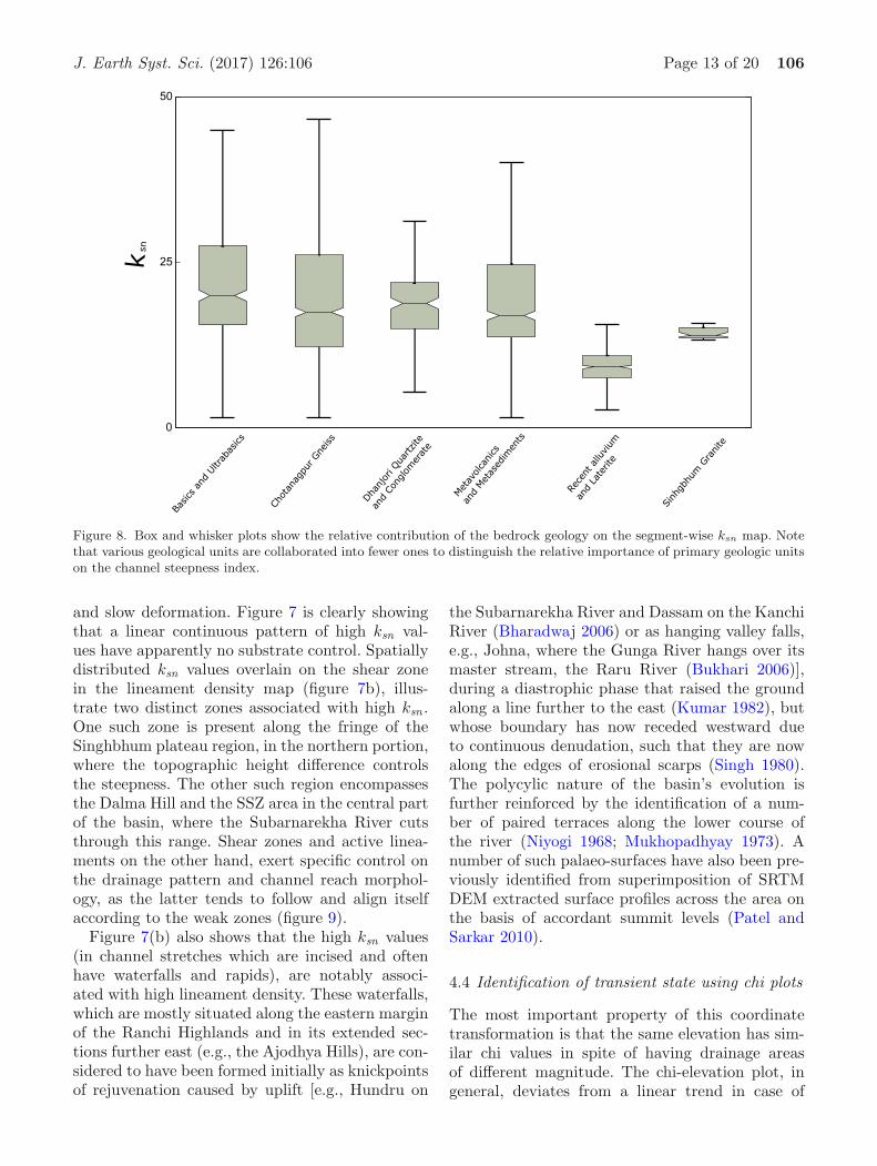
It is evident from figure 8 that recent alluviumand laterites give rise to notably low ksn valueswhich are constricted to the downstream or lowerpart of the basin. However, apparently, there isno systematic strong lithological control on thechannel steepness as the median and interquartilerange is similar in most of the substrate forma-tions except for the Singhbhum granite (figure 8).The Kharkai basin is underlain by this uniformgranite terrain which exhibits prolonged erosionand relatively stable topography. The ChotanagpurGneissic Complex depicts the most heterogeneousdistribution of ksn which is a sign of persistent

106 Page 12 of 20 J. Earth Syst. Sci. (2017) 126:106

a

b

a

b

Figure 7. Lithological and structural control on the channel steepness. (a) Spatially varying ksn values overlain on thelithology map. (b) Lineament density map underlain by the spatially varying ksn values.

J. Earth Syst. Sci. (2017) 126:106 Page 13 of 20 106

Figure 8. Box and whisker plots show the relative contribution of the bedrock geology on the segment-wise ksn map. Notethat various geological units are collaborated into fewer ones to distinguish the relative importance of primary geologic unitson the channel steepness index.

and slow deformation. Figure 7 is clearly showingthat a linear continuous pattern of high ksn val-ues have apparently no substrate control. Spatiallydistributed ksn values overlain on the shear zonein the lineament density map (figure 7b), illus-trate two distinct zones associated with high ksn .One such zone is present along the fringe of theSinghbhum plateau region, in the northern portion,where the topographic height difference controlsthe steepness. The other such region encompassesthe Dalma Hill and the SSZ area in the central partof the basin, where the Subarnarekha River cutsthrough this range. Shear zones and active linea-ments on the other hand, exert specific control onthe drainage pattern and channel reach morphol-ogy, as the latter tends to follow and align itselfaccording to the weak zones (figure 9).

Figure 7(b) also shows that the high ksn values(in channel stretches which are incised and oftenhave waterfalls and rapids), are notably associ-ated with high lineament density. These waterfalls,which are mostly situated along the eastern marginof the Ranchi Highlands and in its extended sec-tions further east (e.g., the Ajodhya Hills), are con-sidered to have been formed initially as knickpointsof rejuvenation caused by uplift [e.g., Hundru on

the Subarnarekha River and Dassam on the KanchiRiver (Bharadwaj 2006) or as hanging valley falls,e.g., Johna, where the Gunga River hangs over itsmaster stream, the Raru River (Bukhari 2006)],during a diastrophic phase that raised the groundalong a line further to the east (Kumar 1982), butwhose boundary has now receded westward dueto continuous denudation, such that they are nowalong the edges of erosional scarps (Singh 1980).The polycylic nature of the basin’s evolution isfurther reinforced by the identification of a num-ber of paired terraces along the lower course ofthe river (Niyogi 1968; Mukhopadhyay 1973). Anumber of such palaeo-surfaces have also been pre-viously identified from superimposition of SRTMDEM extracted surface profiles across the area onthe basis of accordant summit levels (Patel andSarkar 2010).

4.4 Identification of transient state using chi plots

The most important property of this coordinatetransformation is that the same elevation has sim-ilar chi values in spite of having drainage areasof different magnitude. The chi-elevation plot, ingeneral, deviates from a linear trend in case of

106 Page 14 of 20 J. Earth Syst. Sci. (2017) 126:106

Figure 9. Channel morphology, riverbed structures and major waterfalls in the Subarnarekha River Basin with: (a) Insetmap denoting the locations and extents of the various photographs or Google Earth image windows which are as follows.S1: The Hundru Falls on the River Subarnarekha; S2: The Dassam Falls on the River Kanchi; S3: The Jonha Falls on theRiver Gungu; S4: Rectangular jointing on the bed of the Sapahi River at its confluence with the Subarnarekha River justeast of Ranchi; S5: Gouged out channels in bedrock by the Sankha River near Balarampur (Puruliya, West Bengal); S6:Folded gneiss on the Sankha River bed near Balarampur (Puruliya, West Bengal); S7: Steeply dipping foliated metamorphicsat Jamsola which are superposed on by the Subarnarekha River; S8: Quartzite hill ranges of Belpahari which are the easterncontinuation of the SSZ; S9: Wide sandy bed of the Subarnarekha River at Rohini (Paschim Medinipur, West Bengal);W1: The principal folded ranges of the SSZ around Jamshedpur where the Kharkai flows into the Subarnarekha, whichhas a constrained, sinuous bedrock channel along this entire stretch till Jamsola; W2: Change in bed material and channelmorphology of the Subarnarekha after Jamsola, with the river having some meander loops and a broad sandy channel withextensive point and side bars; W3: The Subarnarekha’s final stretch shows a series of meandering loops having alternatingpoint bars.

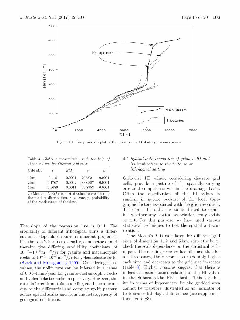
contrasting lithological boundary or a change in therelative uplift rate (Perron and Royden 2013). Fig-ure 10 clearly depicts a drastic deviation from thelinear trend where downstream from the demar-cated knickpoints, the slope of the chi-elevationplot increases. The derived chi values show a tran-sient phase of erosion in the upper region for themain stream and two other tributaries. In gen-eral, there is apparently no significant differencein rock erodibility and other related parametersbetween the upstream and downstream reachesof these knickpoints. The only possibility of the

disequilibrium might thus be a slow, ongoing pro-cess of uplift, whose rate, extent and influence isnot constant spatially. The other tributaries havecollapsed on to the main stream and this is pro-jecting a steady state condition.

Further detailed analysis of statistical derivationconstrains the stream power law more accuratelyas the chi values are plotted with the elevationdata itself, which is less noisy than the slopedata. Regression analysis shows that the m/nratio for the best fit model (R2 = 0.83) is 0.59with the reference drainage area A0 = 1 km2.

J. Earth Syst. Sci. (2017) 126:106 Page 15 of 20 106

Figure 10. Composite chi plot of the principal and tributary stream courses.

Table 3. Global autocorrelation with the help ofMoran’s I test for different grid sizes.

Grid size I E(I) z p

1 km 0.118 −0.0001 207.02 0.0001

2 km 0.1767 −0.0002 83.6387 0.0001

5 km 0.2686 −0.0011 29.8753 0.0001

I : Moran’s I, E(I): expected value for consideringthe random distribution, z: z score, p: probabilityof the randomness of the data.

The slope of the regression line is 0.14. Theerodibility of different lithological units is differ-ent as it depends on various inherent propertieslike the rock’s hardness, density, compactness, andthereby give differing erodibility coefficients of10−7−10−6m−0.2/yr for granite and metamorphicrocks to 10−5−10−4m0.2/yr for volcaniclastic rocks(Stock and Montgomery 1999). Considering thesevalues, the uplift rate can be inferred in a rangeof 0.04–4mm/year for granite–metamorphic rocksand volcaniclastic rocks, respectively. However, therates inferred from this modelling can be erroneousdue to the differential and complex uplift patternacross spatial scales and from the heterogeneity ofgeological conditions.

4.5 Spatial autocorrelation of gridded HI andits implication to the tectonic orlithological setting

Grid-wise HI values, considering discrete gridcells, provide a picture of the spatially varyingerosional competence within the drainage basin.Often the distribution of the HI values israndom in nature because of the local topo-graphic factors associated with the grid resolution.Therefore, the data has to be tested to exam-ine whether any spatial association truly existsor not. For this purpose, we have used variousstatistical techniques to test the spatial autocor-relation.

The Moran’s I is calculated for different gridsizes of dimension 1, 2 and 5 km, respectively, tocheck the scale dependence on the statistical tech-niques. The ensuing exercise has affirmed that forall three cases, the z score is considerably highereach time and decreases as the grid size increases(table 3). Higher z scores suggest that there isindeed a spatial autocorrelation of the HI valuesin the Subarnarekha River basin. This variabil-ity in terms of hypsometry for the gridded areacannot be therefore illustrated as an indicator oftectonics or lithological difference (see supplemen-tary figure S3).

106 Page 16 of 20 J. Earth Syst. Sci. (2017) 126:106

a

b

c

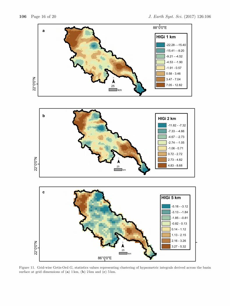
Figure 11. Grid-wise Getis-Ord Gi statistics values representing clustering of hypsometric integrals derived across the basinsurface at grid dimensions of (a) 1 km, (b) 2 km and (c) 5 km.

J. Earth Syst. Sci. (2017) 126:106 Page 17 of 20 106

However, the Gi statistics map depicts welldefined high and low clusters of HI value, whereintwo distinct zones of high HI value cluster havebeen identified (figure 11). The prominent reasonfor the high HI values in these grids is the loweramount of terrain dissection. This less dissectionis generally attributed to either increased tectonicuplift or to the presence of a resistant rock cover.In the upstream region, the distinct and abruptchange in the high HI value cluster zone lies withinthe gneissic terrain, similar in lithology to its sur-roundings, thus implying that it is in fact a slowand steady endogenic perturbation, rather thanlithological differences, which is the driving factorherein. Here the river has also bent sharply to thesouth from its initial eastward direction, possiblyas a result of stream piracy (Mahadevan 2002). Inthe downstream region, there is another cluster ofhigh HI values overlain on the Tertiary and Pleis-tocene sediments. The elevation distribution of thedownstream region is certainly relatively quite low,depicting quite negligible or no regional tectonicuplift. Therefore, this anomalous pattern can beattributed to relatively lesser dissection herein dueto Cenozoic sedimentation and its partial protec-tion by a lateritic duricrust caprock (e.g., as is seenin the Lalgarh formation along the eastern fringeof the basin), along with the presence of NW–SEtrending low hills of schist, phyllite and resistantquartzite. The higher HI cluster here is thus morelithologically induced.

5. Conclusion

The Singhbhum craton is one of the oldest surfacesin the world, with an age of more than 3.12Ga(Misra and Johnson 2005), wherein the documen-tation of more recent tectonic activities is scant. Inthe present study, a thorough analysis of the mor-phometric parameters along with the structuralcharacteristics confirms an ongoing slow tectonicdeformation within the Subarnarekha River basin.The dearth of absolute dating techniques retardsthe quantification of the Quaternary uplift andincision rates, but the overall pattern implies anapparently steady tectonic uplift in the upstreamsections of the drainage area. It is further corrobo-rated with the existing literature that the longitu-dinal profile forms of the streams flowing across thissurface provides one of the most sensitive gaugesof the changes in relative motion and elevationof the surface, as they record these deformations

in terms of anomalies in their respective profiles(Han and Choi 2014), being salient indicators ofneotectonic activity in an otherwise ancient land-scape. These anomalies, as marked by the breaksor knickpoints along these streams’ courses, cor-relate strongly with existing structural and some,albeit much fewer, lithological boundaries as well.The majority of such knicks are observed along thescarp line forming the transition zone between theeastward extensions of the Chotonagpur Plateau’sdissected tracts and ranges, and the lower elevationplains that abut it to the south and east, imply-ing a possible tectonic movement, further modifiedby erosion induced recession of initial fall lines.Their considerable height till today, further demon-strates that uplifting forces are still active overthe Chotanagpur plateau as a whole (Mahadevan2002), reinforcing the need for such investigations.This is ratified by the occurrence of recent earth-quakes, albeit gentle ones, whose foci lie within oraround the periphery of the Subarnarekha Basin(e.g., the 2005 tremor near Ghatshila of magnitude3.8 – information acquired from http://www.isc.ac.uk). Statistical clustering reveals groupings ofhigh and low hypsometric values, implying that thedenudation of this landscape has not been uniform.While this is to be expected, in the light of a raft ofdiverse natural processes acting across a variety oflithologies and thereby resulting in varied erosionalrates, the coupling of this phenomenon with theafore mentioned surmises obtained from the analy-sis of stream profiles, can lead to the postulate thatthe overall landscape has responded in a piece-mealmanner to the uplifts suffered by it. Such piece-meal responses are likely to be governed by locallyvarying thresholds, which may be further delvedinto on basis of more detailed field-based investi-gations. This study, using DEM extracted informa-tion, representing such responses qualitatively andcorrelating them quantitatively with the underly-ing litho-structural matrix, serves to pinpoint theprobable sites of such detailed investigations, whichwould elicit more information on the readjustmentsin an otherwise ancient landscape. As such, thiswork provides both, an insight into the presentstudy area’s geological dynamics and a methodol-ogy that may be applicable to other such areas.

Acknowledgements

The authors gratefully acknowledge the contribu-tion of some students of the Department of Geog-raphy, Presidency University, Kolkata, (namely,

106 Page 18 of 20 J. Earth Syst. Sci. (2017) 126:106

Mr Pranav Pratik, Mr Jayesh Mukherjee, MrSoumik Das and Mr Biman Biswas), who will-ingly provided some of the field photographs of thevarious waterfalls within the Subarnarekha RiverBasin. Authors are grateful to Prof. ChalapathiRao and the anonymous reviewer for their con-structive reviews and suggestions which improvedthe clarity of an earlier version of this paper.

References

Abdullah S N and Abdoh G A 2013 Landsat ETM-7 forlineament mapping using automatic extraction techniquein the SW part of Taiz Area, Yemen; Glob. J. Hum.-Soc.Sci. Res. 13 35–37.

Ahmadi R, Ouali J, Mercier E, Mansy J-L, Lanoe B V-V,Launeau P, Rhekhiss F and Rafini S 2006 The geomor-phologic responses to hinge migration in the fault-relatedfolds in the southern Tunisian Atlas; J. Struct. Geol. 28721–728.

Ambili V and Narayana A C 2014 Tectonic effects on the lon-gitudinal profiles of the Chaliyar River and its tributaries,southwest India; Geomorphology 217 37–47.

Azanon J M, Galve J P, Perez-Pena J V, Giaconia F, Car-vajal R, Booth-Rea G, Jabaloy A, Vazquez M, Azor Aand Roldan F J 2015 Relief and drainage evolution dur-ing the exhumation of the Sierra Nevada (SE Spain): Isdenudation keeping pace with uplift?; Tectonophys. 66319–32.

Banerji A K, Mitra S K and Mukhopadhyaya S C 1970 Tec-tonic sequence in the Sini–Saraikela region, Singhbhumdistrict; Quart. J. Geol. Min. Met. Soc. India 42 141–149.

Bharadwaj K 2006 Physical Geography: Hydrosphere; Dis-covery Publishing House, New Delhi.

Bookhagen B and Burbank D W 2010 Toward a completeHimalayan hydrological budget: Spatiotemporal distribu-tion of snowmelt and rainfall and their impact on riverdischarge; J. Geophys. Res. Earth Surf. 115 F03019.

Bookhagen B and Strecker M W 2008 Orographic barri-ers, high-resolution TRMM rainfall, and relief variationsacross the eastern Andes; Geophys. Res. Lett. 35 L06403.

Brunsden D and Thornes J B 1979 Landscape sensitivity andchange; Trans. Inst. Br. Geogr. 4 463–484.

Bukhari A Z 2006 Encyclopedia of Nature of Geography ;Anmol Publications Pvt Ltd., New Delhi.

Burbank D W and Anderson R S 2011 Tectonic Geomor-phology ; John Wiley & Sons, New Jersey.

Burbank D W, Leland J, Fielding E, Anderson R S, Bro-zovic N, Reid M R and Duncan C 1996 Bedrock incision,rock uplift and threshold hillslopes in the northwesternHimalayas; Nature 379 505–510.

Chatterjee S, Krishna A P and Sharma A P 2014 Geospatialassessment of soil erosion vulnerability at watershed levelin some sections of the Upper Subarnarekha river basin,Jharkhand, India; Environ. Earth Sci. 71 357–374.

Colberg J S and Anders A M 2014 Numerical modeling ofspatially-variable precipitation and passive margin escarp-ment evolution; Geomorphology 207 203–212.

Dandapat K and Panda G K 2013 Drainage and floods in theSubarnarekha Basin in Paschim Medinipur, West Bengal,India – a study in applied geomorphology; Int. J. Sci. Res.4 791–797.

Duncan C, Masek J and Fielding E 2003 How steep arethe Himalaya? Characteristics and implications of along-strike topographic variations; Geology 31 75–78.

England P and Molnar P 1990 Surface uplift, uplift of rocks,and exhumation of rocks; Geology 18 1173–1177.

Flint J J 1974 Stream gradient as a function of order,magnitude, and discharge; Water Resour. Res. 10969–973.

Gassman P W, Reyes M R, Green C H and Arnold J G 2007The soil and water assessment tool: Historical develop-ment, applications, and future research directions; Trans.ASABE 50 1211–1250.

Geomatics P C I 2015 Tutorials; PCI Geomatics, RichmondHill, Cannada.

Giri S, Singh A K and Tewary B K 2013 Source and distri-bution of metals in bed sediments of Subarnarekha River,India; Environ. Earth Sci. 70 3381–3392.

Hack J T 1973 Stream profile analysis and stream-gradientindex; J. Res. U.S. Geol. Surv. 1 421–429.

Han J G and Choi S J 2014 Stream analysis of small drainagebasins in an ancient landform, Korean Peninsula; J. AsianEarth Sci. 95 323–330.

Harbor D and Gunnell Y 2007 Along-strike escarpment het-erogeneity of the Western Ghats: A synthesis of drainageand topography using digital morphometric tools; Geol.Soc. India 70 411–426.

Haviv I, Enzel Y, Whipple K X, Zilberman E, MatmonA, Stone J and Fifield K L 2010 Evolution of verticalknickpoints (waterfalls) with resistant caprock: Insightsfrom numerical modeling; J. Geophys. Res. Earth Surf.115.

Howard A D 1994 A detachment-limited model of drain-age basin evolution; Water Resour. Res. 30 2261–2285.

Howard A D and Kerby G 1983 Channel changes in bad-lands; Geol. Soc. Am. Bull. 94 739–752.

Kale V S, Achyuthan H and Sengupta S 2010 Reconstruc-tion of Late Quaternary Fluvio-sedimentary response ofKaveri and Palar Rivers: based on Chronostratigraphy,Digital Geomorphometry and Remote Sensing Analysis.University of Pune, Pune.

Kale V S and Shejwalkar N 2007 Western Ghat escarpmentevolution in the Deccan basalt province: Geomorphicobservations based on DEM analysis; Geol. Soc. India 70459–473.

Kocal A, Duzgun H S and Karpuz C 2007 An accuracyassessment methodology for the remotely sensed discon-tinuities: A case study in Andesite Quarry area, Turkey;Int. J. Rem. Sens. 28 3915–3936.

Kumar P 1982 Diastrophic forces and their geomorphicexpression in Ranchi Plateau; In: Perspectives in Geomor-phology (ed.) Sharma H S, Concept Publishing Company,New Delhi 4 195–210.

Lee C S and Tsai L L 2010 A quantitative analysis for geo-morphic indices of longitudinal river profile: A case studyof the Choushui River, Central Taiwan; Environ. EarthSci. 59 1549–1558.

J. Earth Syst. Sci. (2017) 126:106 Page 19 of 20 106

Lima A G and Binda A L 2013 Lithologic and structural con-trols on fluvial knickzones in basalts of the Parana Basin,Brazil; J. South Am. Earth Sci. 48 262–270.

Lin Z and Oguchi T 2006 DEM analysis on longitudinaland transverse profiles of steep mountainous watersheds;Geomorphol. 78 77–89.

Mahadevan T M 2002 Text Book Series 14: Geology of Biharand Jharkhand ; Geol. Soc. India, Bangalore.

Mandal S K, Lupker M, Burg J P, Valla P G, HaghipourN and Christl M 2015 Spatial variability of 10 Be-derived erosion rates across the southern PeninsularIndian escarpment: A key to landscape evolution acrosspassive margins; Earth Planet. Sci. Lett. 425 154–167.

Mazumder R, Van Loon A J, Mallik L, Reddy S M,Arima M, Altermann W, Eriksson P G and De S 2012Mesoarchaean–Palaeoproterozoic stratigraphic record ofthe Singhbhum crustal province, eastern India: A systhe-sis; Geol. Soc. London, Spec. Publ. 365 31–49.

Misra S and Johnson P T 2005 Geochronological constraintson evolution of Singhbhum mobile belt and associatedbasic volcanics of eastern Indian shield; Gondwana Res.8 129–142.

Molin P and Corti G 2015 Topography, river network andrecent fault activity at the margins of the Central MainEthiopian Rift (East Africa); Tectonophys. 664 67–82.

Moran P A 1950 Notes on continuous stochastic phenomena;Biometrika 37 17–23.

Mukhopadhyay S C 1977 Geomorphology of a part of thelower Kharkai basin; Geogr. Rev. India 39 248–258.

Mukhopadhyay S C 1973 River terraces of SubernarekhaBasin; Geogr. Rev. India 35 152–170.

Nag S K and Chakraborty S 2003 Influence of rock typesand structures in the development of drainage network inhard rock area; J. Indian Soc. Remote Sens. 31 25–35.

Niyogi D 1968 Morphology of the terraces of the Sub-arnarekha river, India; In: Selected papers 21st Interna-tional Geographical Congress, pp. 84–88.

Ord J K and Getis A 1995 Local spatial autocorrelationstatistics: Distributional issues and an application; Geogr.Anal. 27 286–306.

Patel P P and Sarkar A 2010 Terrain characterization usingSRTM data; J. Indian Soc. Rem. Sens. 38 11–24.

Perez-Pena J V, Azanon J M, Booth-Rea G, Azor A andDelgado J 2009 Differentiating geology and tectonics usinga spatial autocorrelation technique for the hypsometricintegral; J. Geophys. Res. Earth Surf. 114.

Perron J T and Royden L 2013 An integral approach tobedrock river profile analysis; Earth Surf. Process. Landf.38 570–576.

Perumal N V A S, Kak S N and Katti V J 1986 Inte-grated remote sensing approach to uranium explorationin India; In: Atomic Energy Agency (ed.) GeologicalData Integration Techniques: Proc. Technical Commit-tee Meeting of the International Atomic Energy Agency,No. IAEA-TECDOC-472, International Atomic EnergyAgency, Vienna, pp. 131–164.

Phillips J D 1998 Earth surface systems: Complexity, order,and scale; Blackwell Publishers, Oxford.

Prasad A D, Jain K and Gairola A 2013 Mapping of lin-eaments and knowledge base preparation using geomaticstechniques for part of the Godavari and Tapi basins, India:A case study; Int. J. Comput. Appl. 70 39–47.

Prince P S, Spotila J A and Henika W S 2011 Stream captureas driver of transient landscape evolution in a tectonicallyquiescent setting; Geology 39 823–826.

Raj K S and Ahmed S A 2014 Lineament extraction fromsouthern Chitradurga Schist belt using Landsat TM,ASTER GDEM and geomatics techniques; Int. J. Com-put. Appl. 93 12–20.

Rao M G 1962 Investigation of manganese and other mineraloccurrences in Midnapore District, West Bengal, ProgressReport for the Season 1961–1962 (GSI-CHQ-1226); Geo-logical Survey of India, Kolkata.

Reusser L J, Bierman P R, Pavich M J, Zen E, Larsen J andFinkel R 2004 Rapid late Pleistocene incision of Atlanticpassive-margin river gorges; Science 305 499–502.

Saha A K 1994 Crustal evolution of Singhbhum–NorthOrissa, eastern India; Geol. Soc. India Memoir, GeologicalSurvey of India, Kolkata 27 341.

Sangode S J, Meshram D C, Kulkarni Y R, Gudadhe S S,Malpe D B and Herlekar M A 2013 Neotectonic responseof the Godavari and Kaddam rivers in Andhra Pradesh,India: Implications to quaternary reactivation of old frac-ture system; J. Geol. Soc. India 81 459–471.

Sarkar A N 1982 Structural and petrological evolution of thePrecambrian rocks in western Singhbhum, Bihar; Geol.Surv India Memoirs, Geological Survey of India, Kolkata113 97p.

Schwanghart W and Kuhn N J 2010 TopoToolbox: A setof Matlab functions for topographic analysis; Environ.Model. Softw. 25 770–781.

Shankar B, Tornabene L L, Osinski G R, Roffey M, BaileyJ M and Smith D 2016 Automated lineament extractiontechnique for the sudbury impact structure using remotesensing datasets – An update; In: Proc. 47th Lunar andPlanetary Science Conf., Texas 47 1424.

Singh O P 1980 Geomorphology of drainage basins in Pala-mau upland; Recent Trends Concepts Geogr. 1 229–247.

Sklar L and Dietrich W E 1998 River longitudinal profilesand bedrock incision models: Stream power and the influ-ence of sediment supply; In: Rivers over Rock: FluvialProcesses in Bedrock Channels (eds) Tinkler K J andWohl E, American Geophysical Union, Washington D.C.,pp. 237–260.

Snyder N P, Whipple K X, Tucker G E and Merritts D J 2000Landscape response to tectonic forcing: Digital elevationmodel analysis of stream profiles in the Mendocino triplejunction region, northern California; Geol. Soc. Am. Bull.112 1250–1263.

Stock J D and Montgomery D R 1999 Geologic constraintson bedrock river incision using the stream power law; J.Geophys. Res. B104 4983–4993.

Strecker M R, Hilley G E, Arrowsmith J R and Coutand I2003 Differential structural and geomorphic mountain-front evolution in an active continental collision zone: Thenorthwest Pamir, southern Kyrgyzstan; Geol. Soc. Am.Bull. 115 166–181.

Tarboton D G, Bras R L and Rodriguez-Iturbe I 1991 Onthe extraction of channel networks from digital elevationdata; Hydrol. Process. 5 81–100.

Thomas M F 2001 Landscape sensitivity in time and space– an introduction; Catena 42 83–98.

Thornbury W D 1954 Principles of Geomorphology, Wiley& Sons, New York.

106 Page 20 of 20 J. Earth Syst. Sci. (2017) 126:106

Valdiya K S 2001 Tectonic resurgence of the Mysore plateauand surrounding regions in cratonic southern India; Curr.Sci. 81 1068–1089.

Whipple K X and Tucker G E 1999 Dynamics of the stream-power river incision model: Implications for height limitsof mountain ranges, landscape response timescales, andresearch needs; J. Geophys. Res. Solid Earth 104 17,661–17,674.

Whipple K X, Wobus C, Kirby E, Crosby B and Sheehan D2007 New tools for quantitative geomorphology: Extrac-tion and interpretation of stream profiles from digitaltopographic data; Short Course presented at the Geolog-ical Society of America Annual Meeting, Denver, CO.

Willett S D, McCoy S W, Perron J T, Goren L and ChenC Y 2014 Dynamic reorganization of river basins; Science343 1248765.

Willgoose G, Bras R L and Rodriguez-Iturbe I 1991 Acoupled channel network growth and hillslope evolu-tion model: 1. Theory; Water Resour. Res. 27 1671–1684.

Wobus C W, Crosby B T and Whipple K X 2006a Hang-ing valleys in fluvial systems: Controls on occurrence andimplications for landscape evolution; J. Geophys. Res.Earth Surf. 111.

Wobus C W, Whipple K X, Kirby E, Snyder N, Johnson J,Spyropolou K, Crosby B and Sheehan D 2006b Tectonicsfrom topography: Procedures, promise, and pitfalls; Geol.Soc. Am. Spec. Paper 398 55–74.

Yarrakula K, Deb D and Samanta B 2010 Hydrodynamicmodeling of Subernarekha River and its floodplain usingremote sensing and GIS techniques; J. Sci. Ind. Res. 69529–536.

Corresponding editor: N V Chalapathi Rao