‘Every snow ake is di erent’ Investigating the e ect of ...
67
University of Reading School of Mathematics, Meteorology and Physics ‘Every snowflake is different’ Investigating the effect of the variability in snowflake shape on aggregation by Victoria J. Heighton August 18, 2008 This dissertation is submitted to the Department of Mathematics and Meteorology in partial fulfilment of the requirements for the degree of Master of Science
Transcript of ‘Every snow ake is di erent’ Investigating the e ect of ...
University of ReadingSchool of Mathematics, Meteorology and Physics
‘Every snowflake is different’
Investigating the effect of the variability insnowflake shape on aggregation
byVictoria J. Heighton
August 18, 2008
This dissertation is submitted to the Department of Mathematics and Meteorology inpartial fulfilment of the requirements for the degree of Master of Science

Abstract
Ice crystal aggregation is of great importance in understanding and predicting precipi-
tation in the UK. It is also highly influential in climate prediction through its influence
on cloud properties. It is therefore important to keep striving for a better understanding
of the mechanism and better methods for its reproduction in models.
Many previous models and studies have assumed relationships on ice particle param-
eters, including fitted area- and mass-diameter relationships. However, these relation-
ships eliminate the variability of these parameters and mean that no account is taken
of the effect of the individual snowflake’s shape.
This dissertation reviews previous research into ice crystal aggregation modelling and
observations. It also investigates the problem using a new modified Monte Carlo model
which employs fall speed equations that are based on the individual particle’s shape, as
every snowflake has its own geometry, and consequently fall speed. Investigation into
the fall speeds showed that the dispersion of the fall speeds between large snowflakes
of different sizes does not reduce to negligible amounts as previously expected in other
studies. This was also reflected in the results on the relationship between the parame-
ters N0 and λ characterising the slope and intercept of the approximately exponential
snowflake size distribution. It was found that λ steadily decreased to values of λ below
10cm−1 contradicting other studies that have suggested that the relationship would alter
dramatically at this point, possibly as a result of aggregation slowing to a negligible rate
through a reduction in the dispersion of fall velocities for large snowflakes. Comparison
with radar data showed that the new modified Monte Carlo model also provided an rea-
sonable reproduction of the obervered approximately exponential relationship between
reflectivity and time.
The results were also compared to results produced by simplified models, employing
fall speed calculations not dependent on individual particle’s shapes. Comparison plots
of the radar reflectivity against time for the models showed that the simplified models
exhibited a much slower aggregation rate. The implications for using data from radar to
observe properties of ice crystals in clouds using Doppler spectra were also investigated.
i

Declaration
I confirm that this is my own work, and the use of all material from other sources has
been properly and fully acknowledged.
Victoria J. Heighton
ii

Acknowledgements
I would like to thank my supervisors Chris Westbrook for his patience, enthusiasm and
support and Robin Hogan for his valuable contributions. I would like to acknowledge
the financial support of the NERC for the Masters programme 2007-08. I would also
like to thank my family for their unending support and love and my friends for always
helping me keep my mind on happier, shinier things.
An Outdoor Hum for Snowy Weather
“The more it snows
(Tiddly Pom)
The more it goes
(Tiddly Pom)
The more it goes
(Tiddly Pom)
On snowing.
And nobody knows
(Tiddly Pom)
How cold my toes
(Tiddly Pom)
How cold my toes
(Tiddly Pom)
Are growing.”
A.A.Milne
iii

Contents
1 Ice Crystals, Snow Flakes and Aggregation 1
1.1 Why is it important? . . . . . . . . . . . . . . . . . . . . . . . . . . . . . 1
1.2 Nucleation . . . . . . . . . . . . . . . . . . . . . . . . . . . . . . . . . . . 2
1.3 Growth mechanisms . . . . . . . . . . . . . . . . . . . . . . . . . . . . . 3
1.4 Ice crystal types . . . . . . . . . . . . . . . . . . . . . . . . . . . . . . . . 3
2 Snowflake fall speeds and aggregation 6
2.1 Observations and modelling of ice particle fall velocities . . . . . . . . . . 7
2.1.1 Observational studies . . . . . . . . . . . . . . . . . . . . . . . . . 7
2.1.2 Theoretical treatment of the ice particle’s fall speed . . . . . . . . 10
2.2 Observations of aggregation in ice clouds . . . . . . . . . . . . . . . . . . 15
2.3 Other Models of ice aggregation . . . . . . . . . . . . . . . . . . . . . . . 18
2.3.1 Passarelli’s 1978 model . . . . . . . . . . . . . . . . . . . . . . . . 18
2.3.2 Snow Growth Model(SGM) . . . . . . . . . . . . . . . . . . . . . 19
2.3.3 A Monte Carlo Model of aggregation . . . . . . . . . . . . . . . . 21
3 A refined Monte Carlo model of aggregation 26
3.1 Mass Diameter relationships . . . . . . . . . . . . . . . . . . . . . . . . . 27
3.2 Velocity Diameter Relationships . . . . . . . . . . . . . . . . . . . . . . . 29
3.3 Diameter - time relationship . . . . . . . . . . . . . . . . . . . . . . . . . 32
3.4 N0 - λ . . . . . . . . . . . . . . . . . . . . . . . . . . . . . . . . . . . . . 33
3.4.1 Moments . . . . . . . . . . . . . . . . . . . . . . . . . . . . . . . . 34
3.4.2 Integrating the size distribution . . . . . . . . . . . . . . . . . . . 36
3.4.3 Other Studies . . . . . . . . . . . . . . . . . . . . . . . . . . . . . 39
3.5 Calculating Radar Observables . . . . . . . . . . . . . . . . . . . . . . . 41
4 Investigating the influence of velocity dispersion 45
4.1 Comparison with a simplified velocity-mass relationship . . . . . . . . . . 46
iv

CONTENTS v
4.2 Effect of velocity dispersion on Doppler radar measurements . . . . . . . 47
5 Conclusions 50
5.1 Summary . . . . . . . . . . . . . . . . . . . . . . . . . . . . . . . . . . . 50
5.2 Possible further work . . . . . . . . . . . . . . . . . . . . . . . . . . . . . 54
Bibliography 55

List of Figures
1.1 Some examples of ice crystal types, from left to right, hexagonal plate,
bullet rossette and dendrite, taken from [25] and [26] . . . . . . . . . . . 4
1.2 Some examples of aggregates, from left to tight, dendrite aggregate,
snowflakes composed of dendrite aggregates, needle-like crystal aggregate,
taken from [30] and [32]. . . . . . . . . . . . . . . . . . . . . . . . . . . . 4
1.3 Diagram depicting the conditions, in temperature and humidity, in which
various ice crystal types form, taken from [32] . . . . . . . . . . . . . . . 5
1.4 Examples of plate ice crystals growing by vapour deposition on the end
of column ice crystals, taken from [33] . . . . . . . . . . . . . . . . . . . 5
2.1 Best Fit curves for velocity-diameter relationship as shown in [13, p. 2194] 8
2.2 Best fit curves for the mass-diameter relationship as shown in [13, p. 2194] 9
2.3 Boundary layer view of an ice particle . . . . . . . . . . . . . . . . . . . 11
2.4 The dashed line represents equation (2.8) and its approximations (2.15),
(2.16) and (2.17) are given by the straight solid lines, taken from [5, p.
1715] . . . . . . . . . . . . . . . . . . . . . . . . . . . . . . . . . . . . . . 13
2.5 Figure taken from [5, p. 1639] illustrating the different Re-X relationships
produced . . . . . . . . . . . . . . . . . . . . . . . . . . . . . . . . . . . . 14
2.6 Plots of particle trajectories for a steady state line source, top plot, and
time-dependent line source, bottom plot, taken from [16, p. 698] . . . . . 16
2.7 N0-λ evolutions from three separate spirals, taken from [13, p. 702] . . . 17
2.8 Predicted relationship between N0 and λ by SGM, taken from [18, p. 11] 20
2.9 To sample collisions a rate of close approach is formulated, this image is
taken from [2] . . . . . . . . . . . . . . . . . . . . . . . . . . . . . . . . . 22
2.10 The fractal dimension df as a function of α, circles are data from the
simulation, taken from [2]. Note the physical values of α are between 1/2
and 1 . . . . . . . . . . . . . . . . . . . . . . . . . . . . . . . . . . . . . . 24
vi

LIST OF FIGURES vii
3.1 Diagram of parameters . . . . . . . . . . . . . . . . . . . . . . . . . . . . 27
3.2 Plot of Mass-Diameter relationship for 5 runs with different random seeds 28
3.3 Mass-diameter relationships from runs with different values for parame-
ters (n, t/2a,Df , t,W, seed) listed run a to e: (5000, 0.1, 605, 20e− 6, 10, 1948),
(10000, 0.1, 800, 20e− 6, 10, 1983), (7500, 0.1, 750, 25e− 6, 10, 1946), (5000, 0.15, 500, 20e− 6, 10, 1911),
(2500, 0.1, 650, 20e− 6, 10, 1578). . . . . . . . . . . . . . . . . . . . . . . . 29
3.4 Plot of Mass-Diameter relationship from Figure 3.2 on logarithmic scales,
the solid black line indicates a m ∝ D2 relationship . . . . . . . . . . . . 30
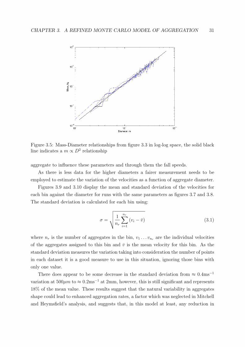
3.5 Mass-Diameter relationships from figure 3.3 in log-log space, the solid
black line indicates a m ∝ D2 relationship . . . . . . . . . . . . . . . . . 31
3.6 Mean velocity-Diameter plots for varied runs, using the same parameter
values as figure 3.3 . . . . . . . . . . . . . . . . . . . . . . . . . . . . . . 32
3.7 Plot of velocity against mass for individual aggregates, with n = 10000,
t/2a = 0.1, Df = 800 and t = 20x10−6 . . . . . . . . . . . . . . . . . . . 33
3.8 Plot of velocity against mass for individual aggregate, with n = 7500,
t/2a = 0.1, Df = 750 and t = 25x10−6 . . . . . . . . . . . . . . . . . . . 34
3.9 Mean and Standard deviation of velocity, with n = 10000, t/2a = 0.1,
Df = 800 and t = 20x10−6 . . . . . . . . . . . . . . . . . . . . . . . . . . 35
3.10 Mean and Standard Deviation of velocity, with n = 7500, t/2a = 0.1,
Df = 750 and t = 25x10−6 . . . . . . . . . . . . . . . . . . . . . . . . . . 36
3.11 A typical plot of average Diameter against time produced by the model . 37
3.12 Size Distribution evolution example in log-linear space . . . . . . . . . . 38
3.13 Evolutions of N0 and λ estimated in different runs using moments 4 to 9 39
3.14 Evolution of cumulative size distribution . . . . . . . . . . . . . . . . . . 40
3.15 Using results from figure 3.14 and basic fitting produces this N0-λ rela-
tionship . . . . . . . . . . . . . . . . . . . . . . . . . . . . . . . . . . . . 41
3.16 Time series from data taken using 8.6mm radar at Chilbolton observatory
on 15.01.08 . . . . . . . . . . . . . . . . . . . . . . . . . . . . . . . . . . 42
3.17 Image of the Galileo (left) and Copernicus (right) radars at Chilbolton
observatory in Hampshire. The data in this study is taken from Coper-
nicus, the 8.6mm radar. This image is taken from [37] . . . . . . . . . . . 42
3.18 Plot 10log10M2 against time for different conditions, the pink dashed, line
represents a linear fit of the relationship . . . . . . . . . . . . . . . . . . 43
3.19 Radar data for reflectivity with fitted linear relationships (pink), mea-
sured 15 January 2008 at 4-4.30 (right) and 4.30-5.30 (left), the melting
layer is shown at approximately 7250 seconds (left) 9500(right) . . . . . . 44
LIST OF FIGURES viii
4.1 The plots and fitted power law relationships are shown for mean velocity
against mass, mean area against radius and mean mass against radius. . 47
4.2 Plot of M2 vs time for the three models using variable values n = 50000,
t/2a = 0.1, t = 20× 10−6 W = 10 finishing at 2500 seconds . . . . . . . . 48
4.3 Plot of results of ‘normal’ and v (m) fitted Doppler spectrum . . . . . . . 49

Chapter 1
Ice Crystals, Snow Flakes and
Aggregation
This first chapter aims to provide the background knowledge on which this project
is based or direct the reader to where it can be obtained. This chapter will provide
an overview to the relevance of aggregation to the weather and climate, though ice
nucleation and growth processes in clouds.
1.1 Why is it important?
Modelling and understanding what happens to ice crystals in clouds is integral to fur-
thering our understanding and ability to model the weather and the climate.
Correctly predicting precipitation is of paramount importance for many things from
agriculture to flood warnings in towns and shipping forecasts and this in turn depends on
the understanding of the processes which create it. In the United Kingdom the majority
of the rain that falls is attributable to melting ice particles. This is due to the Bergeron
Findeisen Process, see section 1.2, which occurs where a small number of ice crystals
grow large at the expense of liquid water droplets. The large ice crystals then fall and
become an efficient source of precipitation and furthermore can seed liquid clouds.
It is also important for improving modelling and understanding the climate. At any
point in time around 1/4 of the surface of the earth is covered by cirrus clouds [23] which
are composed of ice crystals and aggregate snowflakes. The climatic effect of cirrus clouds
is in general a warming. As seen in the Intergovernmental Panel on Climate Change
(IPCC)’s fourth assessment report [27, p. 38], clouds are one of the biggest uncertainties
in predictions of climate change. Deep stratiform ice clouds associated with weather
1

CHAPTER 1. ICE CRYSTALS, SNOW FLAKES AND AGGREGATION 2
fronts could have a cooling effect due to their optical thickness, reflecting solar radiation
back into space. Therefore it is important to understand the growth of ice crystals in
these clouds in order to predict their radiative properties better. Sensitivity studies with
the ECMWF global forecast model have shown that changes in the parameterised ice
particle fall speeds, within a realistic range, can have a large impact changing the global
mean net flux by as much as 10Wm−2, as seen in [28, fig. 1]. It is also important to
improve ice particle aggregation modelling as it is an important growth mechanism, and
increases the fall speeds because of this.
1.2 Nucleation
Ice clouds form as moist air rises in the atmosphere. The associated fall in pressure
causes the air to expand adiabatically and to cool. As the air becomes supersaturated
water droplets are formed on cloud condensation nuclei, of which the atmosphere has
an ample supply. If the droplet is cooled to a sufficiently low temperature then it will
freeze, forming an ice crystal by one of two mechanisms: homogeneous nucleation and
heterogeneous nucleation.
In general homogeneous nucleation is reserved for clouds where the temperature is
−40◦C or lower and as such is mainly the reserve of high clouds like cirrus. For the
droplet to freeze through homogeneous nucleation, some of the water molecules within
the droplet must form into an ice-like lattice structure. If this happens by chance then
the droplet then freezes around these lattice structures. Experimental observations
have shown that this occurs at ≈ −40◦C for the size of droplets that are relevant to the
atmosphere [29].
Heterogeneous nucleation however can occur when the temperature is above −40◦C
and requires the presence of aerosols to serve as a nucleus around which freezing can
occur. Only certain substances are effective as an ice nuclei and this includes clay par-
ticles and desert dust; artificial nuclei include silver iodide and dry ice, the latter being
the basis of cloud seeding. The effectiveness of ice nuclei increases as the temperature
reduces. Due to the relative sparseness of ice nuclei, ice crystals formed through het-
erogeneous nucleation and supercooled water droplets co-exist in clouds. However this
situation can result in the Bergeron Findeisen Process which occurs because the satura-
tion vapour pressure over ice is always greater than that over liquid water. This causes
the ice crystal to grow in the water saturated conditions, which depletes the available
water vapour, making the air subsaturated with respect to the water droplets, which
causes them to evaporate. Thus the ice crystals grow large at the expense of the water

CHAPTER 1. ICE CRYSTALS, SNOW FLAKES AND AGGREGATION 3
droplets.
1.3 Growth mechanisms
Initially the ice crystals grow by the deposition of water vapour onto the surface of the
ice crystal. This dominates the growth of the particle near the top of the cloud where
the ice crystals are small and have small fall speeds. As the crystals get larger and they
begin to fall through the cloud their growth is often dominated by aggregation. Aggre-
gation occurs when ice crystals collide and may form a bond attaching them to each
other therefore forming an ‘aggregate’. The mechanics involved in the bond are still a
matter of research. Sticking mechanisms that have been suggested include: mechani-
cal interlocking, sintering, vapour deposition, electrical forces also known as attraction
and a ‘sticky’ liquid-like layer on the surface of the ice crystal. In older observational
studies it was suggested that ice crystal aggregation became inefficient in temperatures
< −20◦C. However, as improvements have been made in the imaging probes used to ob-
tain measurements from aircraft, aggregates have been found at temperatures of −40◦C
and below [26]. In [30] Mason suggests that the bonding between ice crystals is in part
due to interlocking and to sintering, where the surface attempts to minimise surface
energy in the places the crystals touch forming a bridge between the crystals. Mason
further suggests that if the air surrounding the two particles is supersaturated over ice
then vapour deposition on the surface of the crystals ‘may act as cement’ [30, p. 249].
In [30] the assumption, that aggregation is not efficient at temperatures below −20◦C,
is further dispelled with references to a study by Hosler et al [31] where adhesion of ice
spheres are measured at temperatures down to −80◦C. Aggregate formation is not the
only possible outcome of two ice crystals colliding, they may simply change paths or
break on impact.
There is one other mechanism by which ice crystals can grow and that is riming.
This is when the falling ice crystal gains size as supercooled water droplets in its path
deposit upon it. This dissertation will concentrate only on the growth of ice crystals in
glaciated clouds by aggregation, where bonds between crystals are formed on impact,
figure 1.2 shows some examples of aggregates.
1.4 Ice crystal types
There are many different ice crystal types, described by their geometrical appearance,
degree of riming and degree of aggregation.

CHAPTER 1. ICE CRYSTALS, SNOW FLAKES AND AGGREGATION 4
Figure 1.1: Some examples of ice crystal types, from left to right, hexagonal plate, bulletrossette and dendrite, taken from [25] and [26]
Figure 1.2: Some examples of aggregates, from left to tight, dendrite aggregate,snowflakes composed of dendrite aggregates, needle-like crystal aggregate, taken from[30] and [32].
Figure 1.1 shows some example of different crystal types and figure 1.2 has images
of examples of aggregates of different crystal types.
There are several different categorisation systems which generally focus in particular
on one aspect. Different types are usually identified in studies using images, and data
for different types is usually treated separately.
Different types of ice crystal are known to grow at different temperatures and hu-
midities as shown in figure 1.3. Planar growth, of plates and dendrites, is seen in tem-
peratures between approximately −10◦C and −20◦C. Columns are observed to grow
in approximate temperature regimes of < −20◦C and −3◦C to −10◦C. Plates are also
observed growing for temperatures above −3◦C. The more complex ice crystals shapes
of the branched and dendritic types grow at higher supersaturations. Bullet rossettes
and side planes form at the coldest temperatures below −20◦C.
As a crystal grows larger it begins to fall, which sometimes will take the crystal into
a different temperature regime. This can cause a mixture of crystal types, like plates

CHAPTER 1. ICE CRYSTALS, SNOW FLAKES AND AGGREGATION 5
Figure 1.3: Diagram depicting the conditions, in temperature and humidity, in whichvarious ice crystal types form, taken from [32]
growing on the end of column crystals as seen figure 1.4.
Figure 1.4: Examples of plate ice crystals growing by vapour deposition on the end ofcolumn ice crystals, taken from [33]

Chapter 2
Previous observations and
modelling of snowflake fall speeds
and aggregation
In this chapter I hope to familiarise the reader with previous work on the subject of
ice crystal aggregation both in observation and modelling. Previous models and their
results are clearly very important in order to build a basis on which to build future
improved models, however, observational studies are also very important for models
and modelling. They serve as a benchmark against which a model’s accuracy can be
measured. As modelling techniques and models improve and have greater refinement
there is a demand for increasingly detailed observational measurements and less fallible
techniques and instrumentation.
This chapter firstly provides a review of previous work on aggregation, particularly
those which relate to the fall speeds of ice particles. These are particularly important
as the fall speeds control the aggregation process through collisions produced by ice
particles falling at different velocities. Then observational measurements, taken from
aircraft, of snowflakes in stratiform clouds are also reviewed, to give indication of the
effect of aggregation on ice particle size distributions, and suggestions for what other
processes may be occurring in those clouds. The final part of this chapter shall detail
and discuss how other studies have attempted to model the process.
6
CHAPTER 2. SNOWFLAKE FALL SPEEDS AND AGGREGATION 7
2.1 Observations and modelling of ice particle fall
velocities
2.1.1 Observational studies
In their 1974 [13] Locatelli and Hobbs claimed that although experimental observations
had been gathered before, the data sets available were “still scatty and inadequate for
many purposes” and some “show inconsistencies” with an overall pattern not yet obvious
[13, p. 2185].
Locatelli and Hobbs measured the fall speed of particles using two parallel light
beams placed vertically above one another. Any decrease in the intensity of either
beam is recorded as the passing of the ice particle through that beam. As the exact
distance between the two beams is known the time difference between a particle passing
through the first and the second beam can be used to calculate its fall speed. A thin
piece of plastic, ‘Handiwrap’ below the beams was used to catch the particles so other
observations could be made. The dimensions of the particles were then taken using
microphotographs and after the particles were melted the size of the remaining water
droplet (or sometimes droplets in the case of aggregates) enabled an estimate of the
mass to be obtained.
Through an advance in data gathering technique, there are still potential problems.
It is possible for two particles to be passing through the beams at the same time and
though this can be monitored and any data from such an occurrence ignored, it makes
the method very time consuming. The possibility of a very large particle crossing both
beams at once is negated by separating the two beams by twice as much as the dimension
of the largest particle. Although Locatelli and Hobbs highlight the problem of having
too many classifications of ice particles, they use the same classification system, Magono
and Lee [14], as the problem was highlighted in.
The study did produce some important general patterns within the data for different
particle types. With enough data for a particular particle type, the physical properties
were presumed to fit a relationship of the form y = axb and a logarithmic conversion
of the data was used to find a and b. For most of the particle types studied, Locatelli
and Hobbs produced an estimated relationship for velocity-dimension, velocity-mass and
mass-dimension which can be found in the table in [13, p. 2188].
In comparing their findings with those of other studies Locatelli and Hobbs look at a
study by Zikmunda and Vali [15]. In this study a basic relationship of y = a+ blogD is
assumed rather than y = axb. By using graphical representations of these relationships
CHAPTER 2. SNOWFLAKE FALL SPEEDS AND AGGREGATION 8
and the gathered data for particular particle types, Locatelli and Hobbs argue that their
assumption is closer to reality than Zikmunda and Vali.
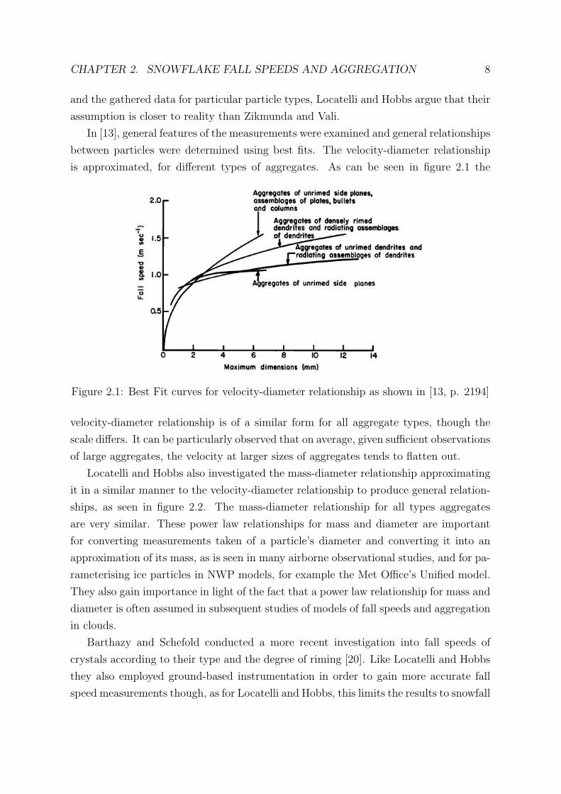
In [13], general features of the measurements were examined and general relationships
between particles were determined using best fits. The velocity-diameter relationship
is approximated, for different types of aggregates. As can be seen in figure 2.1 the
Figure 2.1: Best Fit curves for velocity-diameter relationship as shown in [13, p. 2194]
velocity-diameter relationship is of a similar form for all aggregate types, though the
scale differs. It can be particularly observed that on average, given sufficient observations
of large aggregates, the velocity at larger sizes of aggregates tends to flatten out.
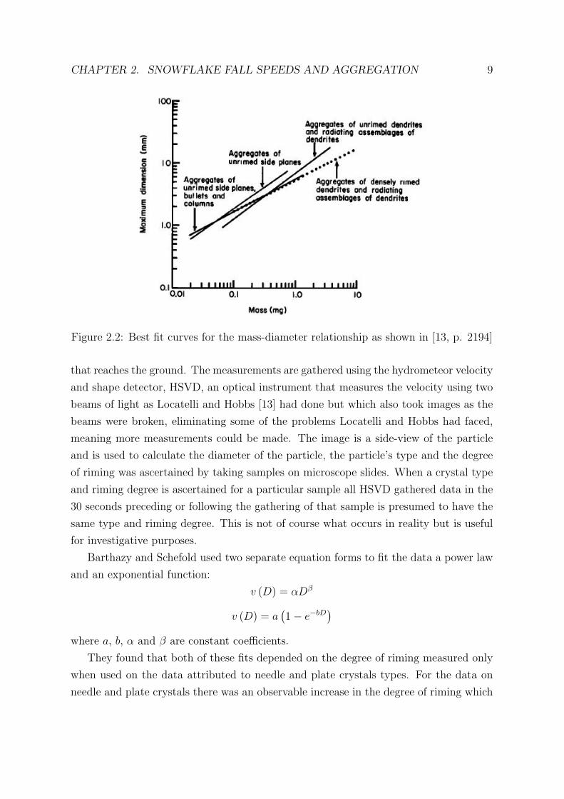
Locatelli and Hobbs also investigated the mass-diameter relationship approximating
it in a similar manner to the velocity-diameter relationship to produce general relation-
ships, as seen in figure 2.2. The mass-diameter relationship for all types aggregates
are very similar. These power law relationships for mass and diameter are important
for converting measurements taken of a particle’s diameter and converting it into an
approximation of its mass, as is seen in many airborne observational studies, and for pa-
rameterising ice particles in NWP models, for example the Met Office’s Unified model.
They also gain importance in light of the fact that a power law relationship for mass and
diameter is often assumed in subsequent studies of models of fall speeds and aggregation
in clouds.
Barthazy and Schefold conducted a more recent investigation into fall speeds of
crystals according to their type and the degree of riming [20]. Like Locatelli and Hobbs
they also employed ground-based instrumentation in order to gain more accurate fall
speed measurements though, as for Locatelli and Hobbs, this limits the results to snowfall
CHAPTER 2. SNOWFLAKE FALL SPEEDS AND AGGREGATION 9
Figure 2.2: Best fit curves for the mass-diameter relationship as shown in [13, p. 2194]
that reaches the ground. The measurements are gathered using the hydrometeor velocity
and shape detector, HSVD, an optical instrument that measures the velocity using two
beams of light as Locatelli and Hobbs [13] had done but which also took images as the
beams were broken, eliminating some of the problems Locatelli and Hobbs had faced,
meaning more measurements could be made. The image is a side-view of the particle
and is used to calculate the diameter of the particle, the particle’s type and the degree
of riming was ascertained by taking samples on microscope slides. When a crystal type
and riming degree is ascertained for a particular sample all HSVD gathered data in the
30 seconds preceding or following the gathering of that sample is presumed to have the
same type and riming degree. This is not of course what occurs in reality but is useful
for investigative purposes.
Barthazy and Schefold used two separate equation forms to fit the data a power law
and an exponential function:
v (D) = αDβ
v (D) = a(1− e−bD
)where a, b, α and β are constant coefficients.
They found that both of these fits depended on the degree of riming measured only
when used on the data attributed to needle and plate crystals types. For the data on
needle and plate crystals there was an observable increase in the degree of riming which

CHAPTER 2. SNOWFLAKE FALL SPEEDS AND AGGREGATION 10
corresponded to an increase in fall speed. Though the fall speeds of all crystal types and
riming degrees exhibit generally similar relationships in these observations it is necessary
to recall the way in which these types and degrees were attributed to them and how this
may have mixed the data for each to a certain degree. For aggregates, the estimated
power-law velocity-diameter relationships were similar to those of Locatelli and Hobbs
and for the largest unrimed aggregates the velocity appears almost constant on average.
2.1.2 Theoretical treatment of the ice particle’s fall speed
Empirical expressions, often in the form of power laws, for the fall speeds of ice particles
have been estimated from observational data and used in many studies and NWP models,
for example the Met Office model [17].
In his paper [5] published in 1996, Mitchell sets forward an improved method of cal-
culation of the terminal velocity of ice particles from their size and shape and compares
the results with previous studies.
The drag force on a particle in a fluid is given by:
FD =1
2ρav
2ACD (2.1)
where ρa is the density of the air, v the velocity of the particle, A the area projected by
the particle perpendicular to the flow and CD is the drag coefficient. For large Reynolds
numbers Re = DV/νk, e.g. large snowflakes, the drag coefficient is approximately
constant, and Mitchell estimates that in this situation CD = C0 = 0.6. For smaller
Reynolds numbers the drag coefficient is not constant but varies with the Reynolds
number CD = CD (Re).
The terminal velocity, v, can then be calculated by equating the gravitational force
mg with the drag force, thus producing the formula:
v =
(2mg
ρaACD
) 12
(2.2)
Unfortunately CD is itself a function of Re and therefore of v.
In order to avoid this dependence on v in the calculation, Mitchell utilises the Best
or Davies Number, X. The Best Number can be calculated without using v:
X = CDRe2 =2mgρaD
2
Aη2(2.3)
where D is the maximum dimension of the particle, η is the dynamic viscosity, Re the

CHAPTER 2. SNOWFLAKE FALL SPEEDS AND AGGREGATION 11
Reynolds number of the particle. The Best number depends on the projected area, mass
and maximum dimension of the particle.
Given knowledge of the particle shape or measurements of mass, area and the maxi-
mum dimension the best number can be calculated directly. A number of experimental
and observational studies have measured Re-X relationships; Mitchell attempts to unify
them into a single theory. Once Re has been calculated from X, the terminal velocity
can be directly calculated from:
v =ReνkD
=ReρaDη
(2.4)
where ν is the kinematic viscosity and η is the dynamic viscosity.
Boundary layer theory is applied to the problem as hypothesized for a sphere by
Abraham [6]. The particle is assumed to have an attached boundary layer surrounding
it of width δ as shown in Figure 2.3. The ice particle and boundary layer are treated as a
solid body, and the flow around the assembly of the particle with its attached boundary
layer is assumed to be inviscid.
Figure 2.3: Boundary layer view of an ice particle
So we now simply require the drag on the entire assembly, Σ, of the ice particle and
its surrounding boundary layer. From equation (2.1) the drag is:
FD =1
2ρv2C0AΣ (2.5)

CHAPTER 2. SNOWFLAKE FALL SPEEDS AND AGGREGATION 12
where AΣ is the projected area of the ice particle and the attached boundary layer. C0
the drag coefficient is now constant as the flow around Σ is inviscid, corresponding to
νk << 1 and therefore the Reynolds number of the assembly is large. Mitchell assumes
that AΣ can be estimated by:
AΣ = π [req + δ]2 (2.6)
where req is the radius of the sphere equivalent in projected area to that of the ice
particle. Boundary layer theory provides the equation:
δ =δ0req√
Re(2.7)
where δ0 is a constant, as in [5].
Combining equations 2.1, 2.3, 2.6 and 2.7 A general relationship between Re and X
is then produced:
Re =δ2
0
4
(1 +4X1/2
δ20C
1/20
)1/2
− 1
2
(2.8)
This continuous analytical relationship can be used to calculate the terminal velocity,
provided the mass and area-dimensional relationships are known, or can be estimated
with a good degree of accuracy.
Previous observational studies [7], [8] have leaned toward the power-law relationship:
Re = aXb (2.9)
and subsequent fall speed expression:
v =aν
D
(2mD2g
ρaν2A
)b(2.10)
Mitchell proposes a simple method to parameterise the Best number, using mass and
area projected normal to the flow expressed in the form of a power law of the maximum
dimension:
m = αDβ (2.11)
A = γDσ (2.12)
So obtaining the expression:
X =2αgρaD
β+2−σ
γη2(2.13)

CHAPTER 2. SNOWFLAKE FALL SPEEDS AND AGGREGATION 13
Based on equation (2.8) the Re-X relationship can be approximated by:
Re = 0.04394X0.970, 0.01 < X ≤ 10.0 (2.14)
Re = 0.06049X0.831, 10 < X ≤ 585 (2.15)
Re = 0.2072X0.638, 585 < X ≤ 1.56x10⁵ (2.16)
Re = 1.0865X0.499, 1.56x10⁵ < X ≤ 108 (2.17)
Though (2.8) is a continuous function it can be approximated using this series of power
Figure 2.4: The dashed line represents equation (2.8) and its approximations (2.15),(2.16) and (2.17) are given by the straight solid lines, taken from [5, p. 1715]
laws over a limited range.
So these parameters can be input as a and b into the equation derived from (2.11),
(2.12) and (2.10):
v = aν
(2αg
ρaν2γ
)bDb(β+2−σ)−1 (2.18)
with α, β, γ and σ dependent on the projected area and mass of the particle. A table
compiled from several sources is contained in the paper [5] containing values for the
parameters dependent on the particle type and its size.
Mitchell and Heymsfield published refinements to the method in 2005 [9]. They
made a minor correction to the method for turbulent flow around aggregates at very

CHAPTER 2. SNOWFLAKE FALL SPEEDS AND AGGREGATION 14
high Reynolds numbers. This only has implications for the very largest ice particles
however.
Mitchell and Heymsfield compared several different Re-X relationships from dif-
ferent studies: The second highest (short dashed) curve in Figure (2.5) represents
Figure 2.5: Figure taken from [5, p. 1639] illustrating the different Re-X relationshipsproduced
Khvorostyanov and Curry’s solution [10]. They expressed (2.8) in the form of a power
law Re = a (X)Xb(X) using parameters equivalent to δ0 = 9.06 and C0 = 0.292, which
Mitchell and Heymsfield argue are more appropriate for modelling smooth rigid spheres
like water drops than ice particles and aggregates. Heymsfield et al. [11] used mea-
surements of aggregates to propose a Re-X relationship that suggested that equation
(2.8) overestimates the fall speeds of the largest snowflakes by 15%. However, Mitchell
and Heymsfield [9, p. 1638] suggest that caution needs to be exercised towards these
measurements due to possible systematic bias in the measurement of the projected area.
This Re-X relationship is illustrated in Figure 2.5 by the lowest (dotted) line though the
possible bias would effect it by overestimating the area and therefore underestimating
the Best number, X. The second lowest (solid) line is produced by (2.8) with δ0 = 5.83
and C0 = 0.6 as used in Mitchell’s 1996 paper [5]. Mitchell and Heymsfield hypothesise
that deviations of the lowest (dotted) line from the second lowest (solid) line are due to
alterations in δ0 and/or C0, since for X > 106 CD ≈ C0 ≈ 0.6 [12], it is likely that these

CHAPTER 2. SNOWFLAKE FALL SPEEDS AND AGGREGATION 15
alterations are in δ0. From (2.8) an increase in δ0 for aggregates could account for a
decreased Reynolds number with respect to the Best number as the lowest line in Figure
(2.5) from [11] suggests, it would also produce an increase in the effective area of the
assembly Σ in boundary layer theory and therefore a decrease in the terminal velocity.
For aggregates Mitchell and Heymsfield propose the following altered relationship
for aggregates:
Re =δ2
0
4
(1 +4X1/2
δ20C
1/20
)1/2
− 1
2
− a0Xb0 (2.19)
where for a0 = 1.7 × 10⁻³ and b0 = 0.8. This equation provides the best fit to the
available fall speed data and is the fall speed equation that will be used in modelling the
aggregation of ice crystals in chapter 3. The additional second term in the equation is
proposed to account for the dilation of δ0 and subsequent increase in the effective area
as they found simply adjusting constants δ0 and C0 was not sufficient.
The Monte Carlo model in section 2.3.3 and chapter 3 resolves the geometry of the
aggregates, therefore the mass, the projected area and the maximum dimension are all
known and need not be estimated by power-law relationships as it is in other studies.
The Best number can be calculated using (2.3) and the Reynolds number by (2.19).
Then the terminal velocity can be calculated using the relationship (2.4) rearranged to
give υt = Reν/D = Reρa/Dη.
2.2 Observations of aggregation in ice clouds
Lo and Passarelli Jr.’s 1982 study [16] was published as an attempt to produce observa-
tional data that could give a 4-dimensional (in space and time) picture of the properties
of the ice crystals throughout their growth history. A major constraint on the solution
of this problem is that all the data be gathered by just one aeroplane in just a single
flight. Another question is whether the technology will be able to differentiate between
the effects of different physical processes.
Another significant factor in the development of the sampling procedure is the hor-
izontal movement of particles exhibited by all ice particles even in steady conditions.
To produce a simple model of this behaviour, assuming a steady, finite source, Lo and
Passarelli used the equation:
X = X0 +S
2
(Z0 − Z)2
v(2.20)

CHAPTER 2. SNOWFLAKE FALL SPEEDS AND AGGREGATION 16
where X is the particle’s horizontal position with respect to its origin X0, S is the
shear, Z is the particle’s below position with respect to its origin Z0 and v is the fall
speed. However as different size particles have different fall speeds this impacts on the
horizontal advection they undergo. Using only two different fall speeds Lo and Passarelli
demonstrate graphically how the advection experienced by one set of particles of one
size is different than that experienced by a set of larger particles, however there is an
overlap between these regions as seen in figure 2.6.
Figure 2.6: Plots of particle trajectories for a steady state line source, top plot, andtime-dependent line source, bottom plot, taken from [16, p. 698]
This means that given a steady, finite source there will be a finite region in which
horizontal advection can be ignored and the particle growth can be measured as a 1-
dimensional problem. Similarly through modelling a source which produces ice particles
for only a limited time it can be shown that even if a source is not steady there will always
be a region which acts as if the source were in a steady state. Using these two findings
Lo and Passarelli surmised that the problem of a horizontally finite, time-dependent
source could be reduced to 1-dimension if the aeroplane were to follow these regions,
which correspond to a infinite, steady source and no horizontal advection, described.
This all presumes finite limits on the fall speeds, which for aggregates [13] suggests is
entirely plausible.
Using this modelled behaviour as a guide, Lo and Passarelli proposed a spiral flight
path where the fall speed and horizontal drift attempted to match that of the average
particle. If the ideal conditions were met, with the diameter of the loops remaining
smaller than the area over which the observed atmospheric properties were uniform
and the overall condition was as steady as possible, then the flight path is known as
the advecting spiral descent (ASD). ASD is designed to be relative to the movement
of the air rather than the aircraft’s position geographically simplifying the problem as

CHAPTER 2. SNOWFLAKE FALL SPEEDS AND AGGREGATION 17
Lagrangian co-ordinates simplify many problems in fluid dynamics in a way Eulerian
co-ordinates would be too cumbersome to do. The data gathered was collected using a
Particle Measuring Systems (PMS) 200-Y probe which took 1-dimensional laser images.
These were then used to count and size the particles.
The results gathered suggested a size-spectrum approximately of the form:
N (D) = N0e−λD (2.21)
where N (D) ∆D is the concentration of particles in the size range [D,D + ∆D], N0 is
the intercept and λ the distribution slope. Lo and Passarelli focus on the evolution of
parameters N0 and λ as the aircraft descends along its Lagrangian spiral.
Figure 2.7: N0-λ evolutions from three separate spirals, taken from [13, p. 702]
As can be seen in figure 2.7, a general pattern of early growth in N0 and small
decreases in λ, changing into the second stage where N0 decreases as well as λ, before
finally stage three is seen where neither N0 or λ decrease or increase in any significant

CHAPTER 2. SNOWFLAKE FALL SPEEDS AND AGGREGATION 18
way. In figure 2.7 the third spiral is seen to only exhibit behaviour from stages 2 and
3. Lo and Passarelli attribute distinct physical processes to these stages, the first being
possibly deposition growth and the second stage aggregation, where the numbers of
small particles decrease as they collide and are collided with to produce new larger ones.
The third stage is more difficult to attribute, with particle breakup being one possible
candidate. This would mean that if a snowflake gets very large it fragments into smaller
pieces, stopping the size distribution getting broader, and this could cause λ to stop
decreasing at 10cm−1. This last stage is one which is particularly interesting as it
cannot be definitively attributed to any particular physical process without significant
doubt.
2.3 Other Models of ice aggregation
Many models of ice aggregation have been produced, many building on previous studies
and incorporating new advancements in knowledge or techniques.
2.3.1 Passarelli’s 1978 model
In 1978 Passarelli [19] attempted to produce a simple analytical model which would
approximate both vapour deposition and aggregation. He had noted that, although
the methods and technologies involved in gathering observational data on precipitation
had been advancing, the interpretation of these results had not been making the same
progress. Many of his predecessors and contemporaries had been employing numerical
integration of the complex equations that result from the known physical properties of
precipitation. However, this is a very cumbersome and expensive technique and often
produces overly complex and confused results.
Passarelli assumed that the precipitation was steady and within a vertically hetero-
geneous cloud and that the size distribution of the ice particles satisfied:
n (D) = N0e−λD (2.22)
as found by Lo and Passarelli [16] from their aircraft measurements. In order to gain
solutions for N and λ Passarelli solves the two first-order ordinary differential equations
(ODEs) produced by the moment conservation equations for the total mass and the
total radar reflectivity, Z. These two moments may be used to derive N0 and λ, see
section 3.4.2, and the total radar reflectivity is proportional to the second moment of the
mass distribution as seen in section 3.5. In order to simplify the ODEs enough to solve

CHAPTER 2. SNOWFLAKE FALL SPEEDS AND AGGREGATION 19
them the aggregates are assumed to be spherical so that the mass diameter relationship
(2.23) can be used.
m = πρD3/6 (2.23)
where ρ is the density of the individual aggregate. The density is assumed to be constant
as a function of D but this is not consistent with observations, for example Locatelli and
Hobbs found m ∝ D2 which gives ρ ∝ 1/D so (2.23) is possibly an oversimplification.
The fall speeds of the aggregates are also approximated using a power law, v = aDb
as per Locatelli and Hobbs, where the parameters a and b depend on the type of ice
crystals involved in the aggregates. Lastly the precipitation is assumed to be steady
and that any vertical flux in the mass and reflectivity is principally due to the fallspeed.
This results in N0 and λ being solved as functions of height below a set level, though if
the cloud is assumed to be spatially homogeneous then N0 and λ are also functions of
time and can be compared to previous studies results.
This model was used to predict the size distribution of ice particles as a function of
time. Its results were exponential, due to its initial assumption, and therefore appear
linear when plotted on a logarithmic-linear scale. When [19, p. 122] Passarelli com-
pared this to contemporary studies which used numerical integration to model raindrop
coalescence; its results did not capture all the detail of the full numerical integration,
but seemed to give a reasonable approximation. However, this model is an advancement
in taking a new look at the techniques and direction that studies of aggregation could
take.
2.3.2 Snow Growth Model(SGM)
Mitchell, Huggins and Grubisic detailed their derivation of and the results gained from
the SGM in a paper in 2005 [18]. This model was based on analysis started by Passarelli
in [19] as discussed above. Once again the several relationships are assumed including:
n (D) = N0e−λD (2.24)
m = aDb (2.25)
A = αDβ (2.26)
They also solved the moment conservation equations for the concentration and the
total radar reflectivity as part of their derivation of the SGM. The SGM breaks away
from many previous studies and takes supersaturation as its input instead of a vertical
profile of the ice water content and temperature. The SGM produced results on size

CHAPTER 2. SNOWFLAKE FALL SPEEDS AND AGGREGATION 20
distributions that appear to correspond favourably to the observational data as seen
in section 2.2. One interesting analysis from the results was an investigation into the
evolution of N0 and λ. The predicted N0 and λ relationship evolves into approximately
Figure 2.8: Predicted relationship between N0 and λ by SGM, taken from [18, p. 11]
a straight line with a gradient of 2 in log-log space with N0 and λ steadily decreasing
until the last 3 points. This relationship is similar to the observational findings of Lo
and Passarelli [16] which can be seen in figure 2.7. Mitchell et al attribute the power-law
relationship, displayed as a straight line in figure 2.8 to the dominance of aggregation
in this period. The aggregation is hypothesised to keep broadening the size distribution
until the system is dominated by large snowflakes which tend to fall at similar speeds, see
section 2.1. The reduced range of fall speeds leads to aggregation eventually becoming
negligible. This causes the growth to be dominated by deposition which increases λ
steepening the size distribution causing the behaviour in the last 3 plotted points in
the bottom left of figure 2.8, which is a similar cut off point to that found by Lo and
Passarelli of 10cm−1.

CHAPTER 2. SNOWFLAKE FALL SPEEDS AND AGGREGATION 21
2.3.3 A Monte Carlo Model of aggregation
This project is based on the model produced in work by Westbrook et al [1],[2] and [3]
which aimed to model the growth of particles by differential sedimentation in particular,
the aggregation of ice crystals in clouds.
In order to simplify the system the following assumptions were made:
1. the cloud is assumed to be dilute, meaning that the mean free path between the
collisions of clusters is large compared to the average distance between clusters.
This allows the model to ignore spatial correlations and concentrate solely on
individual collisions between pairs of clusters.
2. it is assumed that clusters are randomly orientated and that these orientations do
not change during collisions or close encounters with another cluster.
3. hydrodynamic interaction does not effect the collision trajectories, so any effect of
wakes or boundary layers of a cluster on surrounding clusters are ignored
4. all collisions successfully result in aggregation with a permanent, rigid bond at the
point of initial contact
To sample collisions a rate of “close approach” is formulated:
Consider two clusters, i and j, and ascribe to each a radius ri and rj; these radii
enclose the whole of their respective clusters. Each cluster has a fall speed, vi and vj.
The rate of close approach is then calculated thus:
Γij = π (ri + rj)2 |vi − vj| (2.27)
Pairs of clusters are randomly selected with a probability proportional to Γij. In
this way trajectories in which pairs of particles come close to each other are sampled.
Once a pair is selected, one trajectory from all the possible close approaches is chosen at
random, and the particles are tracked along this. If a collision occurs then the clusters
are aggregated. This method means an unbiased sample of collisions between particles
can be gained.
As has been previously shown in section 2.1.2 in [5] Mitchell showed (2.10) that:
v ∼ νkD
(mD2g
ρaν2kA
)α(2.28)
with 0.5 ≤ α ≤ 1. Westbrook et al assumed that A ∝ D2 based on observational data

CHAPTER 2. SNOWFLAKE FALL SPEEDS AND AGGREGATION 22
Figure 2.9: To sample collisions a rate of close approach is formulated, this image istaken from [2]
and their results on the fractal dimensions of the aggregates from their simulations.
Then substituting this relationship into 2.28 we acquire the equation:
v ∼ νkr
(mg
ρν2k
)α(2.29)
In this equation α is an adjustable parameter and D = 2r.
Initially all the particles are rods, half with length and mass of unity and the other
twice as big and massive. This is so there exists some i and j such that |vi − vj| 6= 0.
Previous studies of aggregation suggest that once sufficient aggregation has occurred
the system is insensitive to initial conditions (so having this divide should not impact
on the results). From other aggregation models an educated guess can be made that as
m, s→∞ behaviour will satisfy this relationship:
nm (t) = s (t)−2 φ
[m
s (t)
](2.30)
s (t) =∑i
m2i /∑i
mi

CHAPTER 2. SNOWFLAKE FALL SPEEDS AND AGGREGATION 23
Where nm is the number of clusters of mass m at time t, S is the characteristic clus-
ter mass and φ is the rescaled distribution and a function of m/s (t). There is some
theoretical justification for assuming (2.30) in Van Dongen and Ernst’s 1985 study [4]
in which they show that (2.30) satisfies the Smoluchowski equation seen below. The
scaling function, φ, in (2.30) was confirmed using the simulation data and comparison
with aircraft measured size distributions. The particle diameter distribution was also
measured in these simulations, and found to be approximately exponential, in agreement
with the observational data presented in section 2.2.
Other models and studies suggest that the clusters produced by aggregation are
likely to be fractal in nature or statistically self-similar. This means that the spatial
correlations within the aggregate are similar across a range of different scales, a power
law scaling relating them. Though in reality aggregates may differ slightly from this,
which can be explained through physical reasoning. As each additional ice crystal that
collides and aggregates with the aggregate it forms a protrusion. These protrusions
are more efficient at colliding and therefore collecting other ice crystals, which leads
to aggregates forming with an open, fractal, structure. The simulation results give a
relationship between the mass and radius of the cluster which agrees with the suggestion
that the clusters are fractal. As a fractal nature would imply, for any cluster it is found
that m ∼ rdf where the fractal dimension df is found to be a function of the parameter
α as shown in figure 2.10. Note that df ≈ 2 for α = 1/2 which corresponds well to
experimental data from Locatelli and Hobbs, who estimated df ≈ 1.9, and Heymsfield
et al who found df ≈ 2.09.
The Smoluchowski equation is often used to describe cluster-cluster aggregation
dnk (t)
dt=
1
2
∑i+j=k
Kijni (t)nj (t)−j=1∑∞
Kkjnj (t) (2.31)
where nk (t) is the number of crystals in the system of mass k at time t and the kernel K
is a symmetric matrix where element Ki,j governs the rate of aggregation between pairs
of clusters of masses i and j. This is a simplification of the simulated system since the
aggregation rate is assumed to depend only on particle masses. Then equation (2.27)
may be written as:
Kij ∼∣∣iα−1/df − jα−1/df
∣∣ (i1/df + j1/df)2
(2.32)
Analytical solutions to the Smoluchowski equation have only been found for simple
cases, where Ki,j is constant, i + j or ij. Obviously the Ki,j for this model, equation,
(2.32) is not of this form and an analytical solution was not found.

CHAPTER 2. SNOWFLAKE FALL SPEEDS AND AGGREGATION 24
Figure 2.10: The fractal dimension df as a function of α, circles are data from thesimulation, taken from [2]. Note the physical values of α are between 1/2 and 1
However, substituting (2.30) into the Smoluchowski equation, with the assumption
that average cluster mass, s, is large enough relative to the initial conditions, Van dongen
and Ernst [4] found some properties of solutions. Assuming i << j the elements of the
Kernal scale as:
Kij ∼ iµjν (2.33)
where µ = 0 and ν = α + d−1f for the kernel (2.32).
Westbrook et al then argued that ν = 1 since:
• if ν > 1 then the result is unphysical. The Smoluchowski equation predicts the
formation of a big cluster in zero time. For finite system it is expected that a
few very large clusters will grow very rapidly, which will then dominate the dy-
namics and bond with all of the small particles through aggregation. Through
this aggregation the smaller particles will fill the gaps in the large particles’ struc-
tures making them increasingly compact. This causes df to increase and ν to
subsequently decrease, until the system reaches ν ≤ 1
• if ν < 1 then the result is similar with the feedback increasing ν back to 1. In this
case more collisions occur between similar size clusters which leads to more open
structures. This causes df to decrease and therefore ν to increase.
This argument that ν = 1 was found to be a good fit to the simulation data as shown
by the solid line in figure 2.10. For inertial flow, if α = 1/2 then df = 2, which is in

CHAPTER 2. SNOWFLAKE FALL SPEEDS AND AGGREGATION 25
agreement with observational studies including Locatelli and Hobbs [13].

Chapter 3
A refined Monte Carlo model of
aggregation
The new results presented here were produced using a modified version of the Westbrook
et al Monte Carlo model described in section 2.3.3. The model attempts to simulate
the aggregation of hexagonal plate ice crystals in a deep stratiform ice cloud with an
improved representation of the aggregate fall speed using equation (2.19). Key variables
are defined by the user:
• the initial number of crystals, n.
• the aspect ratio, t/2a, of those crystals, see figure 3.1 where t is the plate thickness
and 2a is the diameter across its hexagonal face.
• the finishing diameter, Df , when the average diameter of all the particles within
the simulation reaches this number the simulation finishes.
• the initial crystal size, t, half the monomers are chosen to have this size, the other
half are twice as big.
• a random seed, to allow the user to produce ‘ensembles’ of different simulations
with the same parameters.
• the wobble, W , the degrees by which the crystals will be able to tilt from the hor-
izontal within the simulation. Experimental data [32] shows that planar crystals
tend to be orientated with their major axes horizontal with a small amount of
wobble, dependent on the Reynolds number. Here it is assumed that the crystal
orientation is uniformly distributed between 0◦ − 10◦.
26

CHAPTER 3. A REFINED MONTE CARLO MODEL OF AGGREGATION 27
Figure 3.1: Diagram of parameters
Other variables are also adjustable by the user however they pertain to more specific
measurements and outputs. We assume that the aggregates are randomly oriented as
they have little symmetry and there is little observational evidence either way.
3.1 Mass Diameter relationships
As discussed in Chapter 2 observational studies are used in the process of assessing
a model’s success in reproducing reality. The relationship between the mass and the
diameter of aggregates frequently forms a fundamental part of these studies. Most
observations suggest a power-law relationship m ∝ Ddf where df is the fractal dimension
as discussed in section 2.3.3.
In order to gauge how the model is predicting this relationship each aggregate is
assigned to a bin according to its diameter after a simulation has run. The number of
particles in each bin and each bin’s collective mass is then ascertained. The model then
outputs this data cataloguing, for each bin, the lowest possible diameter for aggregates
in the bin with the average mass of the aggregates in the bin, using the collective mass
and the number of particles in the calculation. From this we can observe whether the
model is reproducing the observed mass-diameter power-law relationship.
Figures 3.2 and 3.3 show the relationship between the mass and diameter. Firstly
figure 3.2, where the same parameter values are observed with only the random seeds
changed, which provides a sample of the same outcomes for the one set of parameter
values or for one ‘cloud’. Secondly, in 3.3 different parameter values are employed to
give an idea of the sensitivity of the mass-diameter relationship, and consequently the
model, to the different parameters. By looking at both these ways of ‘randomising’ the
results, despite the obvious noise in the plots, we can hopefully be more confident in
the universality of the results. In order to really judge the relationships being produced
here it is best to look at the results on logarithmic scales in log-log space.
As can be seen in the loglog plots in Figures 3.4 and 3.5 the relationship between mass

CHAPTER 3. A REFINED MONTE CARLO MODEL OF AGGREGATION 28
Figure 3.2: Plot of Mass-Diameter relationship for 5 runs with different random seeds
and diameter appears to be approximately m = aDdf where df ≈ 2. This relationship
agrees many of physical observations and studies. In Locatelli and Hobbs [13] it is
estimated that df = 1.9 from data extrapolated from sample aggregates of plates, side
planes, bullets and columns in ground based observations. Aircraft observations by
Heymsfield et al [11] yielded df = 2.04 for aggregates of bullet rosette crystals in cirrus
clouds and df = 2.08 for aggregate of side plane crystals. Mitchell [5] gives estimates of
df between 2.1 and 2.2, depending on the individual crystal types in the aggregation.
This agreement lends support to the model and its close approximation to physical
reality, at least in this fundamental area.
This result also agrees with C.D.Westbrook’s findings in [1], [2] and [3] using the
unmodified model. Westbrook found an approximate relationship of m ∝ D2.05±0.1 for
his simulations and df = 2 from analysis of the Smoluchowski equations for α = 12.
In these studies the approximately quadratic relationship is discussed as a possible
result of the hydrodynamic power law for the particle fall speeds as discussed in section
2.3.3. Those calculations used the less realistic fall speed calculations based on equation
(2.17). The new model presented here uses the full fall speed relationship (2.19) allowing
the particles to span a range of hydrodynamic regimes, and also explicitly includes a
calculation of the projected area rather than simply assuming A ∝ D2 as Westbrook
et al did. This gives us more confidence that we are capturing the physics of the
collisions correctly. Therefore, only the larger particles’ fall speeds are calculated using

CHAPTER 3. A REFINED MONTE CARLO MODEL OF AGGREGATION 29
Figure 3.3: Mass-diameter relationships from runs with different values for param-eters (n, t/2a,Df , t,W, seed) listed run a to e: (5000, 0.1, 605, 20e− 6, 10, 1948),(10000, 0.1, 800, 20e− 6, 10, 1983), (7500, 0.1, 750, 25e− 6, 10, 1946),(5000, 0.15, 500, 20e− 6, 10, 1911), (2500, 0.1, 650, 20e− 6, 10, 1578).
a similar equation to [1]. Yet the mass-diameter relationship still remains approximately
quadratic, this could suggest that this relationship, or at least the methods by which it
is currently studied, is biased towards the larger particles. It is also possible that the
aggregation is largely controlled by the larger crystals capturing the smaller crystals so
the fall speeds of the larger crystals are more influential and control df .
3.2 Velocity Diameter Relationships
The fall speed, in both observation and modeling, holds a significant amount of interest
in modern research into aggregation and many theories are being proposed, tested or
modified in the pursuit of a better understanding of reality. In Mitchell and Heymsfield’s
[9, p.1642] paper and Mitchell et al’s [18] paper they predict that for all aggregates with
large diameters the fall speeds will not differ greatly. This reduction in the dispersion
of fall speeds for larger aggregates is then advocated by Mitchell and Heymsfield as
a reason why aggregation at larger dimensions (approximately ≥ 2mm) may occur at
increasingly negligible rates, in an effort to explain the observations of Lo and Passrelli
in section 2.2 where they found that the size distributions did not broaden further than
λ = 10cm−1.

CHAPTER 3. A REFINED MONTE CARLO MODEL OF AGGREGATION 30
Figure 3.4: Plot of Mass-Diameter relationship from Figure 3.2 on logarithmic scales,the solid black line indicates a m ∝ D2 relationship
The model uses a similar technique as that used to output the necessary informa-
tion for the mass-diameter relationship. The data from aggregates is allotted to bins
according to its diameter and the average velocity for each bin is calculated.
It can be seen in figure 3.6 that the mean velocity for each diameter bin does conform
in general, excluding noise, to the theory that Mitchell and Heymsfield proposed in [9]
and Mitchell et al referenced in [18] with the fall speed flattening out as D increases
past 1mm. However, just looking at the mean velocity is not the whole picture.
Figures 3.7 and 3.8 show the detailed situation, displaying the velocity against the
diameter of each aggregate in the simulation. These figures are just a selection of
what the model consistently produced, which demonstrate that, when the simulation
is run for any significant length, the larger aggregates, with diameters greater than
2mm, have a considerable amount of dispersion in their fall speeds for a given particle
diameter. Similar results can be seen in plots of Locatelli and Hobb’s observational data
[13]. Although the fall speed equations used in the model are those used by Mitchell
and Heymsfield, the model applies them more realistically than in [9]. In [9] area-
and mass-diameter power-law relationships are assumed which are 1-to-1 functions and
predetermined, whereas the model uses each aggregate’s individual area and mass, and
of course ‘every snowflake is different’. The new model presented here is believed to
be more physically realistic in this respect, by allowing the individual geometry of each
CHAPTER 3. A REFINED MONTE CARLO MODEL OF AGGREGATION 31
Figure 3.5: Mass-Diameter relationships from figure 3.3 in log-log space, the solid blackline indicates a m ∝ D2 relationship
aggregate to influence these parameters and through them the fall speeds.
As there is less data for the higher diameters a fairer measurement needs to be
employed to estimate the variation of the velocities as a function of aggregate diameter.
Figures 3.9 and 3.10 display the mean and standard deviation of the velocities for
each bin against the diameter for runs with the same parameters as figures 3.7 and 3.8.
The standard deviation is calculated for each bin using:
σ =
√√√√ 1
nr
nr∑i=1
(vi − v̄) (3.1)
where nr is the number of aggregates in the bin, v1 . . . vnr are the individual velocities
of the aggregates assigned to this bin and v̄ is the mean velocity for this bin. As the
standard deviation measures the variation taking into consideration the number of points
in each dataset it is a good measure to use in this situation, ignoring those bins with
only one value.
There does appear to be some decrease in the standard deviation from ≈ 0.4ms−1
variation at 500µm to ≈ 0.2ms−1 at 2mm, however, this is still significant and represents
18% of the mean value. These results suggest that the natural variability in aggregates
shape could lead to enhanced aggregation rates, a factor which was neglected in Mitchell
and Heymsfield’s analysis, and suggests that, in this model at least, any reduction in

CHAPTER 3. A REFINED MONTE CARLO MODEL OF AGGREGATION 32
Figure 3.6: Mean velocity-Diameter plots for varied runs, using the same parametervalues as figure 3.3
aggregation when aggregates become large is not due to them all having the same fall
speeds.
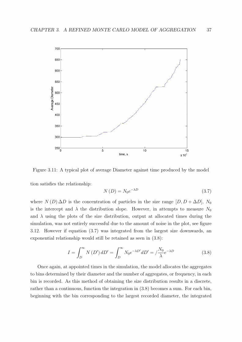
3.3 Diameter - time relationship
Throughout the simulation, every time an aggregation occurs the model calculates the
average diameter, using all particles within the simulation, and then outputs this with
the time. Time within the model is determined for each close approach using equation
(2.27) and the number of clusters left in the simulation.
The average diameter continues to grow throughout the simulation. The points in
the plot corresponding to the lowest diameters can be ignored as they correspond to the
initial monomers and as such are not necessarily physically relevant. From figure 3.11
it appears that growth generally increases in a steady manner. The apparent ‘jumps’ in
time are a product of a finite number of particles in the simulation and a close approach
occurring for a pair of clusters for which the corresponding probability (2.27) was low.

CHAPTER 3. A REFINED MONTE CARLO MODEL OF AGGREGATION 33
Figure 3.7: Plot of velocity against mass for individual aggregates, with n = 10000,t/2a = 0.1, Df = 800 and t = 20x10−6
3.4 N0 - λ
The parameters N0 and λ are often studied and are used to describe the relationship
between the concentration and diameter as has been previously introduced in 2.21. It is
the evolution of these parameters throughout aggregation and therefore our simulation
which is of particular interest. Lo and Passarelli [16] separated the evolution into three
stages discussed in 2.2. Of these sections it is the third that is of the most interest as it
is not yet widely accepted as attributable to any particular mechanism.
It is necessary to attempt to estimate the values of N0 and λ from the data in the
simulation as direct calculation is not possible. This was first attempted by programming
the model to output the size distribution at given points during the simulation.
The example of the evolution of size distribution from the model in figure 3.12 is typ-
ical. Though the size distribution could be exponential for large D, as predicted by the
well-used assumption n (D) = N0e−λ, the noise in the data in these plots overwhelmed
any possible underlying relationship making it impractical to estimate N0 and λ, or
indeed to reliably confirm that n (D) was exponential. Attempts using wider diameter

CHAPTER 3. A REFINED MONTE CARLO MODEL OF AGGREGATION 34
Figure 3.8: Plot of velocity against mass for individual aggregate, with n = 7500,t/2a = 0.1, Df = 750 and t = 25x10−6
bins used to gather the data in the model were unsuccessful in reducing the amount of
noise to the point where a discernible relationship was apparent.
3.4.1 Moments
The next method attempted, with the hope of overcoming the problem of noise, involved
the calculation of moments from the data. The ith absolute moment Mn of a probability
function f (x) about a point a is calculated thus:
Mi =
∫ ∞−∞|x− a|i f (x) dx (3.2)
For the relationship N (D) = N0e−γD, D replaces x, a = 0 and N (D) replaces f (x) in
3.2 and as N is output from the model as a positive discrete function the integration
becomes a summation over all the bins with a lower limit of 0:
Mi =∞∑0
DiN (D) ∆x (3.3)

CHAPTER 3. A REFINED MONTE CARLO MODEL OF AGGREGATION 35
Figure 3.9: Mean and Standard deviation of velocity, with n = 10000, t/2a = 0.1,Df = 800 and t = 20x10−6
However the Mi can also be written as:
Mi = N0
∫ ∞0
Diexp (−λD) dD = N0Γ (i+ 1)
λi+1(3.4)
By equating 3.3 and 3.4 and using Γ (i) = (i− 1)! equations to estimate λ and N0 are
created applicable for any i in the natural numbers:
λ = (i+ 1)Mi
Mi+1
(3.5)
N0 =Miλ
i+1
i!(3.6)
The model output λ and N0 for each individual moment and an average estimate cal-
culated from these for predetermined points in the simulation. However, initial results
were not very successful and appeared to give very little correlation. This was possibly
due to the inclusion of the lower order moments, which are in their calculation weighted
towards the smaller diameter end of the spectrum and the monomers. As this part of

CHAPTER 3. A REFINED MONTE CARLO MODEL OF AGGREGATION 36
Figure 3.10: Mean and Standard Deviation of velocity, with n = 7500, t/2a = 0.1,Df = 750 and t = 25x10−6
the simulation is not yet independent of its initial conditions it is not appropriate or
physically correct to lend such weight to this data. So the model was made to work only
on medium order moments:
In Figure 3.13 the evolutions of N0 and λ in general agree with the second stage
noted by Lo and Passarelli [16], that of a mutual reduction. Some of the plots seem to
exhibit behaviour towards the end that may be consistent with stage 3 though it occurs
at slightly higher values with most studies placing it at around 10cm−1. The lack of
consistency between the different derived N0-λ curves in figure 3.13 may suggest that
either the size distribution was so noisy as to strongly effect the moments used, or that
deviations from the assumed exponential shape N = N0e−λD biased the estimates of N0
and λ.
3.4.2 Integrating the size distribution
Here we will investigate an alternative approach to estimating N0 and λ.
Many studies and models have been based on the assumption that the size distribu-
CHAPTER 3. A REFINED MONTE CARLO MODEL OF AGGREGATION 37
Figure 3.11: A typical plot of average Diameter against time produced by the model
tion satisfies the relationship:
N (D) = N0e−λD (3.7)
where N (D) ∆D is the concentration of particles in the size range [D,D + ∆D], N0
is the intercept and λ the distribution slope. However, in attempts to measure N0
and λ using the plots of the size distribution, output at allocated times during the
simulation, was not entirely successful due to the amount of noise in the plot, see figure
3.12. However if equation (3.7) was integrated from the largest size downwards, an
exponential relationship would still be retained as seen in (3.8):
I =
∫ ∞D
N (D′) dD′ =
∫ ∞D
N0e−λD′
dD′ = /N0
λe−λD (3.8)
Once again, at appointed times in the simulation, the model allocates the aggregates
to bins determined by their diameter and the number of aggregates, or frequency, in each
bin is recorded. As this method of obtaining the size distribution results in a discrete,
rather than a continuous, function the integration in (3.8) becomes a sum. For each bin,
beginning with the bin corresponding to the largest recorded diameter, the integrated

CHAPTER 3. A REFINED MONTE CARLO MODEL OF AGGREGATION 38
Figure 3.12: Size Distribution evolution example in log-linear space
size distribution, I, is calculated by summing the frequency of current bin to the I of its
neighbouring bin. This results in the plot show that much of the noise seen in figure 3.12
is eliminated; this is the advantage of integration where the noise is accumulated and,
to an extent, cancels itself out. The resulting curves in figure 3.14 show that I (D) is
approximately exponential which confirms that n (D) is also approximately exponential,
an important relationship for the model to capture and reproduce.
Figure 3.14 is plotted in log10I-D space which means that the relationship, using
logarithmic rules, becomes:
log10I
log10e=log10
N0
λ
log10e+ logee
−λD (3.9)
log10I = log10N0 − log10λ− (log10e)λD (3.10)
Therefore, a best fit can be used to estimate the gradient from each slope, so it can be
ascribed to − (log10e)λ, the intercept can also be estimated and it is log10N0 − log10λ.
Figure 3.15 shows us a relationship between N0 and λ which, for higher values of
N0 and λ, is as expected and represents the ‘stage 2’ which Lo and Passarelli observed

CHAPTER 3. A REFINED MONTE CARLO MODEL OF AGGREGATION 39
Figure 3.13: Evolutions of N0 and λ estimated in different runs using moments 4 to 9
[16] as it is discussed in section 2.2. However unlike the results produced by Mitchell
et al the relationship continues to values of λ < 10cm−1 = 1000m−1. Mitchell et al’s
prediction for the change in the N0 and λ relationship was based on the similarity of
the velocities of larger particles leading to a reduction in aggregation. This new model,
as had been suggested in 3.2, shows evidence that possibly contradicts Mitchell et al’s
predictions and suggest that aggregation can in principle continue to broaden the size
distribution even when the particles are large.
3.4.3 Other Studies
There are many competing theories on the relationship between N0 and γ particularly
what occurs at around λ = 10cm−1 and what drives this behaviour. Lo and Passarelli
[16] examine the behaviour around λ = 10cm−1 in their observations to find all cease
to evolve, indicating that the a balance within the size distribution has occurred with
smaller particles that aggregate being replaced and the larger particles that aggregation
is producing are reducing in number. Lo and Passarelli propose that this behaviour is
consistent with a mechanism of the largest snowflakes breaking up on impact, which is a

CHAPTER 3. A REFINED MONTE CARLO MODEL OF AGGREGATION 40
Figure 3.14: Evolution of cumulative size distribution
mechanism not included in this new model, though they concede that it could potentially
be the product of instrument-artifact.
Mitchell et al. [18], as discussed in section 2.3.2, used results from their Snow Growth
Model to attempt to validate the Mitchell and Heymsfield hypothesis, suggesting that
the change between the power-law relationship seen in stage 2 and the more static rela-
tionship in stage 3 was due to aggregation ceasing to be the dominant growth mechanism
for the ice crystals. This would mean that the velocities of larger ice crystals would have
to be very similar making the possibility of collision and therefore aggregation negligible.
However, the present study has shown that there may still be significant dispersion in
the fall speeds of larger ice crystals, see section 3.2.
More recently studies have emerged that support an instrument-based explanation
for the behaviour of N0 and γ. Korolev and Isaac’s 2004 study [21] and Field et al’s
2006 study [22] both investigate the hypothesis that Optical Array Probes (OAP) and
High Volume Precipitation Spectrometers (HVPS) have been providing incorrect data
for observational studies due to the shattering of particles on the instruments. When
a large particle shatters on the probe inlet, its contribution to n (D) is lost but the
smaller pieces of it that remain could be counted by the optical probes. In many earlier
observational studies this process was not known of so any readings from the shattered

CHAPTER 3. A REFINED MONTE CARLO MODEL OF AGGREGATION 41
Figure 3.15: Using results from figure 3.14 and basic fitting produces this N0-λ relation-ship
particles would not to be rejected from a study and it could cause there to be a skew in
the data, especially further into the aggregation process or equivalently lower down the
cloud where the particles are larger. This could possibly account for the behaviour seen
later on in the evolution of the N0-γ plot, as suggested by Heymsfield et al in [34], who
argues the true values of λ continue to decrease past ≈ 10cm−1.
3.5 Calculating Radar Observables
Another method of measurement frequently employed in Meteorology is radar. Doppler
radar is sensitive to the concentration, size, fall speed and types of hydrometers including
ice crystals, within clouds. Radars emit pulses of radiation, typically between 3mm
and 10cm in wavelength, and Rayleigh scattering by the snowflakes leads to some of
the wave being reflected back, and the intensity and time taken are measured by the
radar. An example time series from a vertically pointing 8.6mm radar at the Chilbolton
observatory in Hampshire is shown in figure 3.16 and the radar is pictured in figure 3.17.
It is possible to see a thick stratiform ice cloud with rain at the ground and the cloud
top at 8000m to 9000m for the time period studied in this dissertation, 0300-0800 hours.
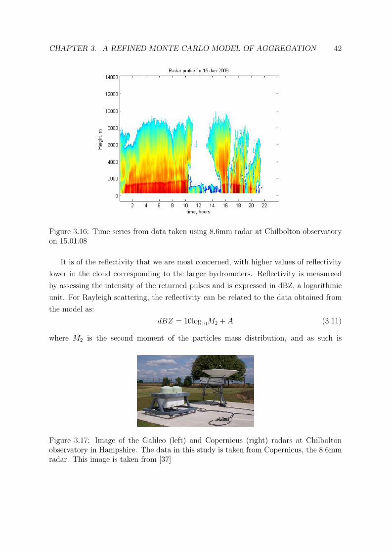
CHAPTER 3. A REFINED MONTE CARLO MODEL OF AGGREGATION 42
Figure 3.16: Time series from data taken using 8.6mm radar at Chilbolton observatoryon 15.01.08
It is of the reflectivity that we are most concerned, with higher values of reflectivity
lower in the cloud corresponding to the larger hydrometers. Reflectivity is measureed
by assessing the intensity of the returned pulses and is expressed in dBZ, a logarithmic
unit. For Rayleigh scattering, the reflectivity can be related to the data obtained from
the model as:
dBZ = 10log10M2 + A (3.11)
where M2 is the second moment of the particles mass distribution, and as such is
Figure 3.17: Image of the Galileo (left) and Copernicus (right) radars at Chilboltonobservatory in Hampshire. The data in this study is taken from Copernicus, the 8.6mmradar. This image is taken from [37]

CHAPTER 3. A REFINED MONTE CARLO MODEL OF AGGREGATION 43
weighted towards the larger snowflakes, and A is a constant calculated by:
10log10
(36 |Kice|2
0.93π2ρ2ice
)
as seen in [35]. The Doppler velocity, vd, is also measured which is equivalent to the
average speed that the particles are moving towards the radar.
Figure 3.18: Plot 10log10M2 against time for different conditions, the pink dashed, linerepresents a linear fit of the relationship
Comparison of the general form of the results with radar data can be undertaken,
however, a numerical comparison of the absolute dBZ values would be meaningless due
to the unknown scale of ice production at the cloud top. The similarity in the shape of
these plots supports the fact that the initial conditions on the ice crystals in the model
do not affect the result in figure 3.18 and we observe that the second moment of the
mass distribution grows approximately exponentially with time.
Figure 3.19 is constructed by the method outlined in Westbrook et al’s paper [35].
The highest data point with a measurable reflectivity in the vertical profile is taken to
be the height of the cloud top, htop, which is presumably where the ice is formed. From
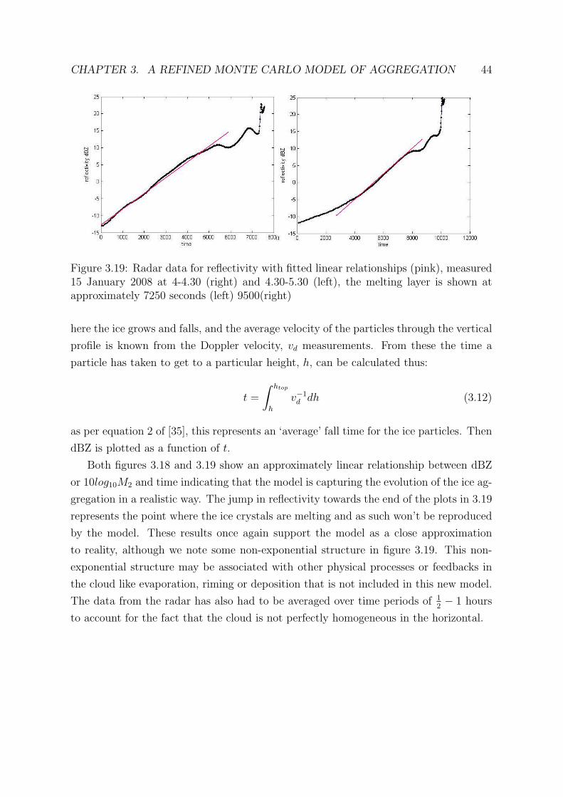
CHAPTER 3. A REFINED MONTE CARLO MODEL OF AGGREGATION 44
Figure 3.19: Radar data for reflectivity with fitted linear relationships (pink), measured15 January 2008 at 4-4.30 (right) and 4.30-5.30 (left), the melting layer is shown atapproximately 7250 seconds (left) 9500(right)
here the ice grows and falls, and the average velocity of the particles through the vertical
profile is known from the Doppler velocity, vd measurements. From these the time a
particle has taken to get to a particular height, h, can be calculated thus:
t =
∫ htop
h
v−1d dh (3.12)
as per equation 2 of [35], this represents an ‘average’ fall time for the ice particles. Then
dBZ is plotted as a function of t.
Both figures 3.18 and 3.19 show an approximately linear relationship between dBZ
or 10log10M2 and time indicating that the model is capturing the evolution of the ice ag-
gregation in a realistic way. The jump in reflectivity towards the end of the plots in 3.19
represents the point where the ice crystals are melting and as such won’t be reproduced
by the model. These results once again support the model as a close approximation
to reality, although we note some non-exponential structure in figure 3.19. This non-
exponential structure may be associated with other physical processes or feedbacks in
the cloud like evaporation, riming or deposition that is not included in this new model.
The data from the radar has also had to be averaged over time periods of 12− 1 hours
to account for the fact that the cloud is not perfectly homogeneous in the horizontal.

Chapter 4
Investigating the influence of
velocity dispersion on aggregation
Two other papers have considered the effects of velocity dispersion on aggregation, the
first by Passarelli and Srivastava [38] and the second by Sasyo and Matsuo [39]. However,
the new modified Monte Carlo model employed in this dissertation has the advantage
over these previous studies as it explicitly resolves the shape of individual particles. Like
many previous studies, including Passarelli, as seen in section 2.3.1 and Mitchell et al,
as discussed in section 2.3.2, these two studies both assumed the existence of a 1-to-1
relationship between particle mass and diameter. They did however use an assumed
probability distribution of different fall speeds as a function of D in the calculation of
the collision rate. This produced a dispersion in the velocity that was uniform around
the mean. Both studies found that the effect of variability in the fall speeds was to
increase the growth rate significantly. Passarelli and Srivastava also discovered that the
size spectrum broadens and reflectivity increased.
Mitchell et al stated in their 2006 paper [18] that their results supported a hypothesis
that the rate of aggregation slows to such a negligible rate when a particle’s diameter gets
large that it appears to stop. This has been previously discussed in sections 2.3.2 and 3.2.
It is based on the theory that for large particles the dispersion of fall speeds is very small
and as such Ki,j ∝ |vi − vj| (Di +Dj)2, which corresponds to the rate of aggregation
between two particles i and j, is very small. However, results from this model have
shown the evidence to support the idea that the dispersion between fall speeds for large
particles is not negligible, see figures 3.7 - 3.10. For large particles however, (Di +Dj)2
is large and so only a small dispersion in the velocities may be needed, thus |vi − vj| 6= 0,
for a reasonable rate of aggregation. Therefore it is necessary to investigate whether
calculating the fall speeds of individual particles based on geometry, and therefore not
45

CHAPTER 4. INVESTIGATING THE INFLUENCE OF VELOCITY DISPERSION46
stopping aggregation for larger particles as is done in the model, produces very different
results than if a simpler relationship was used to calculate the fall speed as Mitchell et
al did in [18].
4.1 Comparison with a simplified velocity-mass re-
lationship
There are two ways in which the calculation of a particle’s velocity can be simplified to
the level used in many studies. The first is to use a simple power law of the form v = amb
and the second is to use power laws for the mass-radius and area-radius relationships
which can be substituted into the velocity equations already in use in the model, thereby
eliminating any dependence of the velocity on an individual particle’s geometry.
In order to produce a 1-to-1 velocity-mass relationship, against which the model can
be tested, the full simulation is run with a given set of conditions and the velocities
and masses of each particle output. This allows a best fit to be found and from this
a velocity-mass relationship for the conditions can be established. The simpler model,
S1, is then produced as exactly the same as the original model but with all velocity
calculations replaced by a simple function of mass.
The 1-1, power-law, mass-radius and area-radius relationships are found using a sim-
ilar method. The second simpler model, S2, is produced by inputting dummy variables
for the radius and area as a function of mass into the fall speed equation, (2.19). The
dummy variables are constructed using the power law relationships for mass against
radius and area against radius.
The averaged plots and fitted power-law relationships are shown in figure 4.1 for one
arbitrarily chosen simulation. The assumption of a power-law relationship appears to
fit well with the data; however, it is the model’s sensitivity to this assumption which is
of interest to us.
In figure 4.2 it is obvious that the results from the simpler models, S1 and S2, have
a much slower growth. This is as previous studies, including those by Passarelli and
Srivastava [38] and the second by Sasyo and Matsuo [39], predicted. It is also physically
intuitive: as the dispersion in velocities between the particles of larger sizes increased so
did their probability of collision and consequently aggregation, therefore greater numbers
of aggregations are likely to take place as are collisions between larger particles, which
have a significant impact on the results. This second moment, proportional to the radar
reflectivity, is used to compare the new modified Monte Carlo model with the simpler
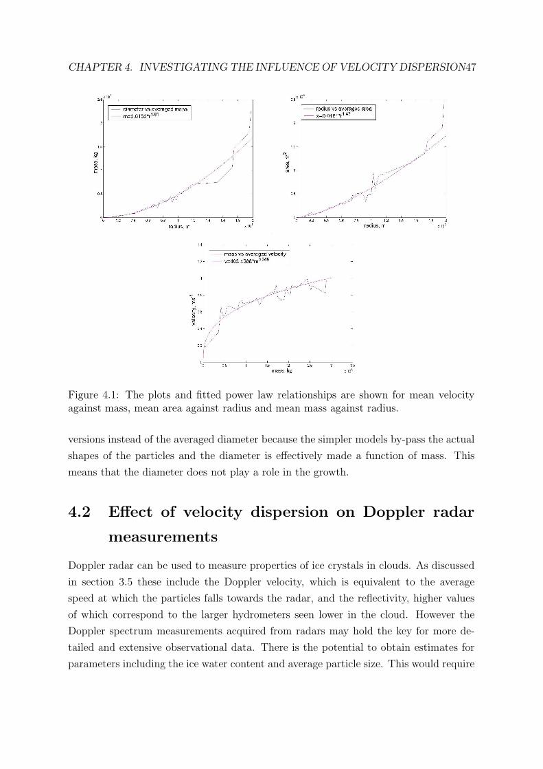
CHAPTER 4. INVESTIGATING THE INFLUENCE OF VELOCITY DISPERSION47
Figure 4.1: The plots and fitted power law relationships are shown for mean velocityagainst mass, mean area against radius and mean mass against radius.
versions instead of the averaged diameter because the simpler models by-pass the actual
shapes of the particles and the diameter is effectively made a function of mass. This
means that the diameter does not play a role in the growth.
4.2 Effect of velocity dispersion on Doppler radar
measurements
Doppler radar can be used to measure properties of ice crystals in clouds. As discussed
in section 3.5 these include the Doppler velocity, which is equivalent to the average
speed at which the particles falls towards the radar, and the reflectivity, higher values
of which correspond to the larger hydrometers seen lower in the cloud. However the
Doppler spectrum measurements acquired from radars may hold the key for more de-
tailed and extensive observational data. There is the potential to obtain estimates for
parameters including the ice water content and average particle size. This would require

CHAPTER 4. INVESTIGATING THE INFLUENCE OF VELOCITY DISPERSION48
Figure 4.2: Plot of M2 vs time for the three models using variable values n = 50000,t/2a = 0.1, t = 20× 10−6 W = 10 finishing at 2500 seconds
assumptions: that a relationship between the velocity and mass exists and that the size
distribution follows a known function, probably exponential. We therefore must check
whether making these assumptions in this situation is reasonable or if assuming the
velocity can be calculated using a simple velocity-mass relationship produces an altered
spectrum.
To test this, the summation of the mass squared,∑m2, will be studied as a function
of the velocity. The Doppler spectrum, which is ∝∑
binm2/bin width as a function of
v, is produced using the assumed 1-to-1 velocity mass fit and is compared with the
‘real’ spectrum where all the variability of different snowflake shapes are taken account
of. To produce a plot of this without the assumptions, a ‘normal’ output, the particles
will be allocated to bins according to their velocity. The mass for each particle is then
squared and added to the∑m2 that corresponds to its velocity-designated bin. The
total∑m2 for each bin is then plotted against the velocity. To assume the relationship
between velocity and mass a ‘simplified’ output is calculated. The particles are binned
by mass, rather than velocity, and each particle’s mass is squared and added to the∑m2 corresponding to the bin. Before the data collected for each bin is output by the

CHAPTER 4. INVESTIGATING THE INFLUENCE OF VELOCITY DISPERSION49
model the velocity is calculated assuming the velocity-mass relationship. This is done
using the method for a velocity-mass relationship described for the S2 model in section
4.1.
Figure 4.3: Plot of results of ‘normal’ and v (m) fitted Doppler spectrum
Figure 4.3 shows that the Doppler spectrum produced with and without the under-
lying assumptions. The plots both exhibit noise which is to be expected as all the plots
produced using a method that involved using bins have done so. The general form of the
spectrum, without assuming a velocity-mass relationship, appears to be approximately
parabolic in shape. When a velocity-mass relationship is assumed then the spectrum
produced appears to match the ‘normal’ spectrum in the centre however as the velocity
becomes large the∑m2 does not decrease as expected, but remains at a reasonably
high level. This behaviour was common throughout all attempted parameter variations.
In general the assumptions that are needed to obtain estimates of ice crystal pa-
rameters appear to be reasonable; however the behaviour exhibited for larger velocities
is unexpected. It is possible that this behaviour is an artifact of the method by which
these results where produced within the model but this behaviour is an issue that merits
further investigation.

Chapter 5
Conclusions
5.1 Summary
In this dissertation the effect of the variability in snowflake shape on aggregation was
studied and found to be influential in some results but not all.
A literature review of previous studies on aggregation was used to build the picture
produced so far. Particular attention was paid to studies which related to the fall speeds
of ice particles as the fall speeds control the aggregation process through collisions pro-
duced by ice particles falling at different velocities. Calculations of the fall speed from
Mitchell and Heymsfield [9] were used within a new modified Monte Carlo model to
produce a model that accounted for the effects of individual snowflakes shapes. Obser-
vational studies and results were also reviewed, to be used later for comparison, as were
other models.
The results presented in this dissertation are produced using a modified version of the
Westbrook et al Monte Carlo model described in section 2.3.3. The ice crystals used in
the model are hexagonal plates, this is a compromise as although it has been argued by
Jiusto and Weickmann in [36] that large snowflakes would be expected to predominately
be aggregates of dendritic crystals, this would be very computationally expensive to
model, especially accounting for the individual geometry of each aggregate. The results
shown here and in Westbrook et al [2] suggest that many of the results are insensitive
to the choice of initial crystal. The model also uses an improved representation of the
aggregate fall speed using equation (2.19) so the particles now span a range of flow
regimes rather than all existing in the same one, and their projected area is explicitly
calculated.
The effects of these modifications on the new Monte Carlo model were tested, as
50

CHAPTER 5. CONCLUSIONS 51
was the model’s sensitivity to parameter changes. This was first done by observing the
the mass-diameter relationship. Previous observations and studies, including Locatelli
and Hobbs [13] and Heymsfield et al [11] have suggested that a realistic mass-diameter
relationship would be of the form m ∝ Ddf where df ≈ 2. As shown in section 3.1 with
figures 3.2 to 3.5 this appears to be true within the model irrespective of the parameters
used. Therefore the model has managed to capture an important relationship found in
observational studies.
The plots produced of the size distribution, seen in figure 3.12, could be exponential
in nature as suggested by the generally accepted relationship n(D) = N0exp (−λD).
However the noise in the plots is too great for any definitive conclusions to be made on
this. Integration from the largest particle size downwards allowed the exponential shape
to be confirmed as shown in section 3.4.2.
A large part of this dissertation has tested the results from the new modified Monte
Carlo model against hypotheses and results from other studies. Particular focus has
been paid to the hypotheses that concern the evolution of velocity and aggregation for
larger particles.
The evolution of average diameter through time was also studied as one measure of
the aggregation rate. Figure 3.11 is typical of the plots studied, with steady growth
appearing to continue even as the size distribution gets broader. This contradicts the
study by Mitchell and Heymsfield [9] where they hypothesised that as the size dis-
tribution broadened aggregation would cease to be the dominant growth mechanism.
However as the model only simulates aggregation and a steady growth in the average
diameter is still observed as it becomes large then the rate of aggregation is clearly not
decreasing.
Mitchell and Heymsfield’s hypothesis was based upon the assumption that the dis-
persion of fall speeds between large snowflakes of different sizes reduces to negligible
amounts if their diameters are large enough. While the bin averaged velocity against
diameter plots, as seen in figure 3.6, did seem to conform to this assumption, when a
more detailed picture was investigated it appeared that the situation was more complex.
Plots of fall speeds of individual aggregates against its diameter, as seen in figures 3.7
and 3.8, revealed the prospect that, within this model at least, for larger diameters
the dispersion between fall speeds was not negligible and was produced by variability
in snowflake shape. This was further investigated using measurements of the standard
deviation, as it has no bias on the quantity of data points available for each diameter
bin. The standard deviation of the velocity did decrease as the diameter of the particle
became large. However, as displayed in figures 3.9 and 3.10 it in no way became a neg-

CHAPTER 5. CONCLUSIONS 52
ligible amount. Around the diameter sizes that Mitchell and Heymsfield suggested the
fall speed variability would become negligible the standard deviation remains at almost
20% of the average fall speed.
The relationship between the parameters N0 and λ was also investigated, as this has
been a focus of interest in many studies, including Lo and Passarelli [16] and Mitchell et
al [18]. Several methods were attempted to estimate the evolution of the relationship.
The first of these methods involved plotting the evolution of the size distribution and
produced no real results due to problems with noise. The next method used moments of
the size distribution and was successful in producing a recognisable relationship between
N0 and λ when the lower order moments were ignored. These results showed a relation-
ship that was approximately a power-law which was as expected and in that appeared
to recreate the ‘stage 2’ of N0 and λ evolution as observed by [16] and predicted by the
Snow Growth Model in [18]. However, the ‘stage 3’, to which most study is currently
devoted to and Mitchell et al attributed to a significant reduction in the aggregation
rate, at λ 10cm−1 could not be reached by this method. Using any variation in the mo-
ments within the calculation produced very different N0 − λ curves, indicating that the
method was unreliable. The last method attempted was an estimation of the integration
of the size distribution and a study of its evolution. This method not only reproduced
the afore-mentioned ‘stage 2’ of a power law but continued this relationship past the
marker of λ ≈ 10cm−1 set by Mitchell et al and Lo and Passarelli for the radical change
in behaviour. As this modified Monte Carlo model concentrates solely on aggregation
this suggests that aggregation does not slow significantly which relates well to the results
produced by the model on the dispersion of fall speeds for larger diameters but conflicts
with the hypothesis given in Mitchell et al’s study.
This continuation of the N0 and λ power law relationship for λ < 10cm−1 also con-
flicts with airborne observations produced by Lo and Passarelli [16]. However, Lo and
Passarelli did not attribute the change in the relationship, only suggesting that it may
be due to the break-up of particles, whereas the model is restricted to aggregation, so
another mechanism or feedback may be the cause of the observed ‘stage 3’ behaviour.
Another possibility is that it could be caused by the instrumentation used to gather the
data for [16]. In studies by Field et al [22] and Korolev and Isaac [21] the effects of ice
crystals shattering on the houses of the probes or in the turbulence and wind shear cre-
ated by them in similar experiments are studied. This would mean that the data would
be lost from the observations about many large particles as they shatter but the smaller,
shattered pieces of it could remain and be counted within the observations. These read-
ings would not have been rejected or accounted for, and could cause the observations to

CHAPTER 5. CONCLUSIONS 53
produce incorrect size distributions, especially further into the aggregation process or
equivalently lower down the cloud where there is a greater concentration of large parti-
cles. The effect of particles shattering would be to produce incorrect size distributions
with an increased number of small particles and a decreased number of large particles
than is there in reality, leading to a steeper size distribution and a larger λ that the true
value. This is in its effect analogous to the natural break-up mechanism suggested by
Lo and Passarelli as the cause for the ‘stage 3’ behaviour in their observations. Korolev
and Isaac used an observed correlation between the maximum observed particle size and
the frequency of images containing multiple fragments of particles being observed in the
data to substantiate the idea. Their results suggested that for aggregates, within the
images taken for airborne observations, the percentage of images containing shattered
particles could be as high as 10%. Field et al’s study also suggests that the impact of
the shattering particles on the results would be significant with the difference in con-
centrations in particle size distributions being changed by up to a factor of 4 for some
studies. They also showed evidence that the broader the size distribution became, which
corresponds to the lower values of λ, the greater the effect the shattering would have on
the results. This could possibly explain the results seen in Lo and Passarelli’s results
for N0 and λ as suggested very recently by Heymsfield et al in [34] however it is in no
way certain.
The second moment of the particle mass distribution was used to produce compar-
isons with data on reflectivity, Z taken from the 8.6mm Doppler radar at the Chilbolton
observatory in Hampshire. This parameter has been observed to grow approximately
exponentially with time, as seen in section 3.5, so it appears as a linear relationship on
a logarithmic scale, dBZ units, of the data from the model. The data from the model
is output at 10 ∗ log10M2 which is proportional to dBZ and is observed in figure 3.18 to
also have an approximately exponential relationship with time in agreement with the
radar data, see figure 3.19. This supports Westbrook et al’s [35] hypothesis that this
exponential relationship is a “signature” signature of the mechanism of aggregation.
Lastly the modified Monte Carlo model was compared with simplified versions us-
ing assumptions of power-law relationships that are prevalent in studies on ice crystal
aggregation. The results showed that the simpler models grew at a significantly slower
rate than the new modified Monte Carlo model. This suggests that the effect of the vari-
ability in snowflake shapes is influential and cannot be in general ignored, and suggests
that fitted relationships as used to define many variables in many studies, are possibly
not the best method of snowflake modelling.
The implications of the velocity dispersion on using radar measurements to obtain

CHAPTER 5. CONCLUSIONS 54
more extensive observations on ice clouds was also investigated as this would involve
the assumption of a calculable velocity-mass relationship. The results showed that for
most velocities, and hence diameters, the effect on the Doppler spectrum was not too
discernible. However, for the highest velocities there was an unexpected change with the∑m2 remaining large when to produce the observed parabolic shape it should reduce.
This behaviour is intriguing and merits further investigation.
5.2 Possible further work
As results in this dissertation have shown the dispersion of velocity and its effects merit
further investigation. As well as investigation into the wider issue of its effects the
results have exposed several areas that also merit further study.
More sensitivity tests should possibly be carried out looking at the mass-diameter
relationship and velocity dispersion amongst others.
With further availability of more powerful computational units bigger simulations
could be run to improve the statistics on results like the size distribution.
The behaviour of the Doppler spectrum plot for large velocities is interesting and it
would be interesting to see if it is an artifact of the method used in producing the plot.
Other mechanisms could be built into the model and this could be evaluated to see
how this changes the results and how the mechanisms react to each other. In particular
calculation of the efficiency of aggregation against deposition as a growth mechanism in
various temperature and super-saturation regimes in order to process how these affect
which mechanism is dominant.

Bibliography
[1] Westbrook, C. D., R. C. Ball, P. R. Field and A. J. Heymsfield: Uni-
versality in Snowflake Aggregation Geophysical Research Letters, 31, 2004, L15104.
[2] Westbrook, C. D., R. C. Ball, P. R. Field and A. J. Heymsfield: Theory
of growth by differential sedimentation, with application to snowflake formation
Physical Review, 70, 2004, 021403.
[3] Westbrook, C. D.: Universality in snowflake formation Phd thesis, 2004.
[4] Van Dongen, P. G. J. and M. H. Ernst: Dynamical scaling in the kinetics of
clustering Phys. Rev. Lett., 54, 1985, 1396-1399.
[5] Mitchell, D. L.: Use of Mass- and Area-Dimensional Power Laws for Determin-
ing Precipitation Particle Terminal Velocities Journal of the Atmospheric Sciences,
53, 1996, 1710–1722.
[6] Abraham, F. F.: Functional dependence of drag coefficient of a sphere on
Reynolds number Phys. Fluids, 13, 1970, 2194–2195.
[7] Knight, N. C. and A. J. Heymsfield: Measurement and interpretation of
hailstone density and terminal velocity Journal of the Atmospheric Sciences, 40,
1983, 1510–1516.
[8] Heymsfield, A. J. and M. Kajikawa: An improved approach to calculating
terminal velocities of plate-like crystals and graupel Journal of the Atmospheric
Sciences, 44, 1987, 1088–1099.
[9] Mitchell, D. L. and A. J. Heymsfield: Refinements in the Treatment of Ice
Particle Terminal Velocities Highlighting Aggregates Journal of the Atmospheric
Sciences, 62, 2005, 1637–1644.
55
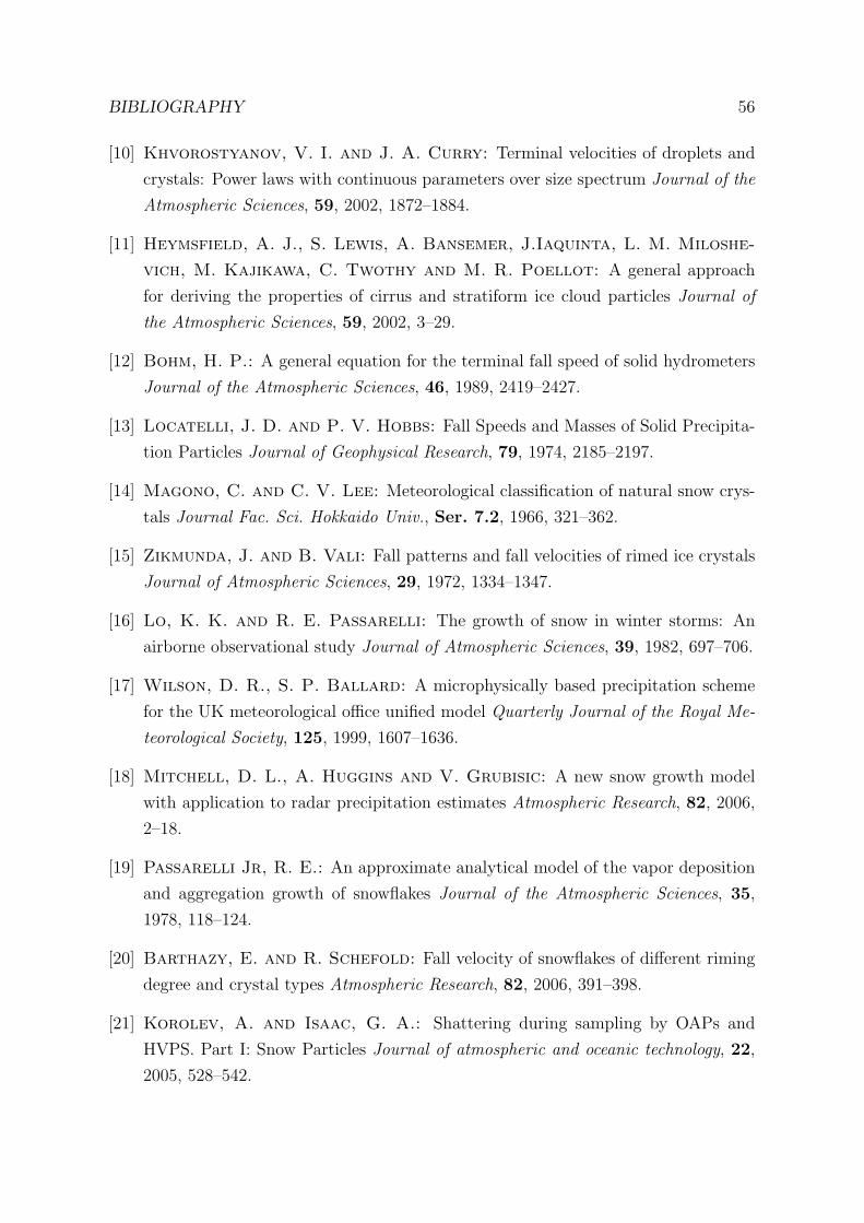
BIBLIOGRAPHY 56
[10] Khvorostyanov, V. I. and J. A. Curry: Terminal velocities of droplets and
crystals: Power laws with continuous parameters over size spectrum Journal of the
Atmospheric Sciences, 59, 2002, 1872–1884.
[11] Heymsfield, A. J., S. Lewis, A. Bansemer, J.Iaquinta, L. M. Miloshe-
vich, M. Kajikawa, C. Twothy and M. R. Poellot: A general approach
for deriving the properties of cirrus and stratiform ice cloud particles Journal of
the Atmospheric Sciences, 59, 2002, 3–29.
[12] Bohm, H. P.: A general equation for the terminal fall speed of solid hydrometers
Journal of the Atmospheric Sciences, 46, 1989, 2419–2427.
[13] Locatelli, J. D. and P. V. Hobbs: Fall Speeds and Masses of Solid Precipita-
tion Particles Journal of Geophysical Research, 79, 1974, 2185–2197.
[14] Magono, C. and C. V. Lee: Meteorological classification of natural snow crys-
tals Journal Fac. Sci. Hokkaido Univ., Ser. 7.2, 1966, 321–362.
[15] Zikmunda, J. and B. Vali: Fall patterns and fall velocities of rimed ice crystals
Journal of Atmospheric Sciences, 29, 1972, 1334–1347.
[16] Lo, K. K. and R. E. Passarelli: The growth of snow in winter storms: An
airborne observational study Journal of Atmospheric Sciences, 39, 1982, 697–706.
[17] Wilson, D. R., S. P. Ballard: A microphysically based precipitation scheme
for the UK meteorological office unified model Quarterly Journal of the Royal Me-
teorological Society, 125, 1999, 1607–1636.
[18] Mitchell, D. L., A. Huggins and V. Grubisic: A new snow growth model
with application to radar precipitation estimates Atmospheric Research, 82, 2006,
2–18.
[19] Passarelli Jr, R. E.: An approximate analytical model of the vapor deposition
and aggregation growth of snowflakes Journal of the Atmospheric Sciences, 35,
1978, 118–124.
[20] Barthazy, E. and R. Schefold: Fall velocity of snowflakes of different riming
degree and crystal types Atmospheric Research, 82, 2006, 391–398.
[21] Korolev, A. and Isaac, G. A.: Shattering during sampling by OAPs and
HVPS. Part I: Snow Particles Journal of atmospheric and oceanic technology, 22,
2005, 528–542.

BIBLIOGRAPHY 57
[22] Field, P. R., A. J. Heymsfield and A. Bansemer: Shattering and parti-
cle interarrival times measured by optical array probed in ice clouds Journal of
Atmospheric and Oceanic Technology, 23, 2006, 1357–1371.
[23] Baran, A. J.: On the scattering and absorption properties of cirrus cloud Journal
of Quantitive Spectroscopy and Radiative Transfer, 89, 2004, 17–36.
[24] Heymsfield, A. J., G-J van Zadelhoff, D. P. Donovon, F. Fabry, R. J.
Hogan and A. J. Illingworth: Refinements to ice particle mass dimensional
and terminal velocity relationships for ice clouds. Parts I and II Journal of the
Atmospheric Sciences, 64, 2007, 1047–1067 and 1068–1088.
[25] http://snowflakebentley.com, Dedicated to Wilson “Snowflake” Bentley’s life’s
work and images, (last checked on 04.08.2008).
[26] Field, P. R., and A. J. Heymsfield: Aggregation and scaling of ice crystal
size distributions Journal for Atmospheric Sciences, 60, 2003, 544–560.
[27] Intergovernmental Panel on Climate Change (IPCC): Climate Change
2007: Synthesis Report, Avaliable from http://www.ipcc.ch, 2007.
[28] A. J. Heymsfield and J. Iaquinta: Cirrus Crystal Terminal Velocities Journal
of Atmospheric Sciences, 57, , 916–938.
[29] Rogers, R. R. and M. K. Yau: A short course in cloud physics, Oxford: Perg-
amon, 1989.
[30] Mason, B. J.: The physics of clouds, Oxford University Press, 1971.
[31] Hosler, C. L., D. C. Jensen and L. Goldshlak: On the aggregation of ice
crystals to form snow Journal of Meteorology, 14, 1957, 415–420.
[32] Pruppacher and Klett: Microphysics of clouds and precipitation, Kluwer Aca-
demic publishers, 1997.
[33] Bentley, W. A., and W. J. Humphreys: Snow crystals, Dover, 1962.
[34] Heymsfield, A. J., P. Field and A. Bansemer: Exponential size distributions
for snow, Journal of Atmospheric Sciences, Not yet published.
[35] Westbrook, C. D., R. J. Hogan, A. J. Illingworth and E. J. O’Connor:
Theory and observations of ice particle evolution in cirrus using Doppler radar:
Evidence for aggregation Geophysical Research Letters, 34, 2007, LO2824.

BIBLIOGRAPHY 58
[36] Jiustoa, J. E. and H. K. Weickmann: Types of Snowfall Bulletin of American
Meteorological Society, 54, 1973, 1148–1162.
[37] http://www.met.rdg.ac.uk/radar/ufam/copernicus.html, The University of
Reading Meteorology department’s radar group’s page on the cloud radars at
Chilbolton, (last checked on 14.08.2008).
[38] Passarelli R. E. Jr, and R. C. Srivastava: A new aspect of snowflake
aggregation theory Journal of Atmospheric science, 36, 1979, 484.
[39] Sasyo Y. and T. Matsuo: Effects of the variations of falling velocities of
snowflakes on their aggregation Journal Met. Soc. Japan, 63, 1985, 249.

![MATHEMATICS OF MEDICAL IMAGING - Whitman vanced Engineering Mathematics [2], ... form/CT data reconstruction and shows the e ect of di erent levels of discrete ... MATHEMATICS OF MEDICAL](https://static.fdocuments.us/doc/165x107/5aab249a7f8b9a693f8b85ff/mathematics-of-medical-imaging-whitman-vanced-engineering-mathematics-2.jpg)